Tschnischs Hochschufs PoSi®cn!co fsderah

Centre Svlzzero di Calcolo Scientifico Eidgsinossische Ecoh po!ytschni<fus f^d^rel® d'a ZurichTschnischs Hochschufs PoSi®cn!co fsderah <S ZurigoZurich Swiss F®dsral Instituts of Twhrwtogy Zurich

c s c sSwiss Scientific Computing Center

to Burgers' Equation

W. Sawyer, G. Kreiss, D. Sorensen and J. Lambers

B—B—

Arnoldi Method Applied to Burgers5 Equation

Abstract:

The Arnold! method for the computation of eigenvalues of large non-symmetric matrices

is applied to Burgers' equation: Ui == (y)_ + £Uxx- The space discretization of the problem

leads to the system of equations v^ = F(v). The asymptotic behavior around the steady state

solution is determined by those eigenvalues of the Jacobian |¥- evaluated at a quasi-steady state

Vg^; which have the smallest negative real part.

Two variants of the Arnold! method are used to find the desired eigenvalues: the basic

algorithm supplemented by two different eigenvalue localizers: polynomial filtering and spectral

transformation. The former is available in the public-domain library ARPACK, while thelatter is problem-specific and is therefore hand-coded. Numerical results are presented and the

relative performance of the two algorithms compared.

William SawyerCSCS-ETH, Section of Research and Development (SeRD),

Swiss Scientific Computing Center,La Galleria, CH-6928 Manno, Switzerland

[email protected]

GuniIIa KreissRoyal Institute of Technology,

Department of Computer Science,

Stockholm, [email protected]

Dan Sorensen

Department of Mathematical Sciences,

Rice University, Houston TX, [email protected]

James Lamb ers

Stanford University,SCCM Program,

Stanford CA, [email protected]

TABLE OF CONTENTS

Table of Contents

1 Introduction2 The Steady State Solution of Burgers' equation ................... 4

3 The Eigenvalues of A ...................•••••••••••••• 7

4 Numerical Calculation of the Eigenvalues of A . ................... 11

4.1 The Arnold! Method ....................•••••••••• n

4.2 Numerical Algorithms to determine the Eigenvalues of A ......... 12

5 Numerical Results .....................•••••••••••••• 16

5.1 Results with Exponential Transformation ..............•••• 16

5.2 Results with Filtering Polynomials ...................... 17

5.3 Comparisons and Conclusions ..................••••••• 20

List of Figures

1 Numerical quasi-steady state

2 Numerical quasi-steady state with "wiggles" ..................... 6

3 Spectral tranformation with exponential function .................. 13

4 Largest eigenvalues as function of Hessenberg matrix size ............. 18

5 Second and third eigenvalues as function of problem size .............. 19

6 Six smallest eigenvalues for problem with "wiggles" ................. 20

7 All eigenvalues of problem with "wiggles" ...................... 21

SeRD-CSCS-TR-94-04

1. INTRODUCTION

1 Introduction

The availability of public-domain software libraries has never been as great as today. The

usefulness of this software, however, is relatively difficult to evaluate, as this software is not

always tested on typical problems in the application user's view.

In this paper, we evaluate a newly available software library eigenvalue solver package,

ARPACK [1] (available from netlib in the SCALAPACK library)1) on a realistic test prob-

lem. We compare the use of ARPACK eigenvalue solvers for a few eigenvalues of a non-

symmetric system, to those of a hand-coded algorithm tailored to this problem.

We consider Burgers' equation:

Ut^>w. + £U^ £ > 0, U(0, <) = -1 u(l, t) = 1 (1)

In order to solve this problem, this equation is discretized in space over n = N — 1 grid

points x, = ih where h = 1/N and i = 0,1,..., N (vio = -1 and VIN = 1), using central

differences we get a system of ordinary differential equations

Vtl =

Vti =

Vtn =

U22 - 1 , V2 - 2Vl - 1

~4h~^£ h2~

V.+l2 - "i-12 , _V,+i - 2u, + v,-i

4h+£-

h2 for 1 < i < n

1-Un2 , _l-2Vn+V»_i

4h +£h2

where n = N — 1

or formulating this more succinctly,

Vt = F(v) (2)

We expect that v = (ui, v^,..., Vn}T where v;(^) approximates u(i/i, (). An analysis of the

discretization error will not be given here — this can be found in standard texts on Numerical

Analysis such as [5].

Of particular interest is the asymptotic behavior around the steady state solution Vg^;. We

therefore let v = Vg^ + v linearize the system about Vg^,

V = Vgt+V

dv 9-FTt = FM^(v,t)+^

/st

(3)

Since ^ = ^ and F(vgt) = 0, this becomes

dv 9¥\dt Qv

The solution to (3) is

A wide variety of software from netlib can be retrieved from the server netlib.ornl.goT. This is best doneusing the facility metlib, which is installed on many UNIX systems.

/st

SeRD-CSCS-TR-94-04

2. THE STEADY STATE SOLUTION OF BURGERS' EQUATION

2 The Steady State Solution of Burgers' equation

We consider the steady state solution to Burgers' equation (1), and integrate once we get the

following equation,

"st'+eu^=C u(0,t)=-l u{l,t) = 1

Equation (2) can be solved by the separation of variables. The general solution for the

zero-centered steady state solution is,

ust = V^'1 tanhC^x-C^)

2e(8)

where C*i and C-t can be determined from the boundary conditions. Note that in this case there

will be symmetry about the point (0.5, 0) thus €2 = 0.5 and Ci can be determined iteratively

for a given e. The following values are accurate to 14 places:

e

0.01250.0250.05

0.1

0.2

_Ci

1.000000000000001.000000004122311.000090721636781.012725616727321.12707885005682

In the general case, of course, an explicit steady state solution is not known. Therefore, as

an exercise, we ignore our knowledge of the exact solution here and attempt to calculate the

steady state solution by discretizing in space, as described previously, and using a time-stepping

algorithm such as Runge-Kutta 4/5 to solve (2) until the change in the grid-function values is

negligible.

While this approach may seem straightforward and seems to lead to adequate results for

many values of N and e (see figure 1), certain anomalous effects can occur: "wiggles" can appear

in numerically calculated steady state solution (see figure 2) if too few grid-points are used.

To explain these wiggles, we consider the semi-discretized equation,

dv, ^ 1 , , ,^ . £^ = °= ^^'+1'' ~ut-1^ + ^^'+1 ~ 2vi + vi~^ (9)

The solution to these difference equations has wiggles if it is not monotonic increasing.

Consider three contiguous grid-function values v,_i, v, and u;+i. Note that in the limiting case

v,+i = v,_i there are no wiggles, as v, = u,+i = u,_i follows immediately from (9).

Now assume two distinct cases (keeping in mind h > 0, e > 0),

• u,+i < u,_i: A wiggle is assured if either v, > v,_i

<==>i::("?+i-^?-i) <8e

h2i >h2l >

v,_i - u.+i

2-2

v._i + u,+i

2

|V.+l+V._l|

SeRD-CSCS-TR-94-04

or if v, < u,4.i,


Af,,2.._,,2^ ^ Vi+l-Vj-18ew+l~v!-l) > ~~T

h>

2e ' u,_i+u,+i

h 2>

Ie ' |u;+i+u,-i|

• U,4-l > 'u»-l we ^ wiggle is assured if either v, > ^,4.1,

Af,,2.__,,2^ ^ Vi+l-Vi-1^W+i~vi-i) > ~~ —g-

h 22e ' u,_i + f,+i

h 22s ' |u,+i+v,-i|

or if v, < v,_i,

^£:(u?+l-u?-l) <v,_i - v;+i

8£'

hIe y._i + u,+i

h 22e ~ ly.+i+v.-il

Thus,

whenever

>2e ' |v.+i+v,-i[

|u,-|.l+Ui-l|is defined.

(10)

Considering (10) it is likely to observe wiggles whenever the right hand side of (10) is small,i.e. where v is still increasing and but has not yet "leveled off". In practice this is exactly where

the wiggles appear (figure 2).From (10) a sufficient condition for the absence of wiggles can be found, namely

h< 2s (11)

The presence of wiggles indicates the qualitative character of the true steady state solution

has been lost in the discrete steady state solution. The use of such a solution in the Arnold! algo-

rithm means virtually anything can happen. For example, it can be shown that the eigenvalues

of A are real if h < 2s, but it can not be shown (and is in reality not true) if h < 2e.

SeRD-CSCS-TR-94-04


N = 200, epsilon = .05, steady-state solution

0 0.1 0.2 0.3 0.4 0.5 0.6 0.7 0.8 0.9 1

Figure 1: Convergence of quasi-steady state solution with £ = 0.05, N = 200

N = 100, epsilon = .001, steady-state solution

0 0.1 0.2 0.3 0.4 0.5 0.6 0.7 0.8 0.9 1

Figure 2: Numerically calculated steady state solution with e = 0.001, N = 100

SeRD-CSCS-TR-94-04

3. THE ESGENVALUES OF A

3 The Eigenvalues of A

It has been shown that if ^ > 1 the numerically calculated values Vg^^ increase monotonically

from -1 to 1 (absence of "wiggles"). We assume monotonicity in the remainder of this section.

In this case, A(,^,_I) and A(,^+I) from (6) are positive. Since the mirrored elements in the

first sub-diagonal have the same sign (+) it is easy to show that the matrix can be diagonally

symmetrized and therefore all the eigenvalues of A are real. In addition, the matrix is nearly

negative diagonally dominant:

u..+i-v,_i , 2e^(i,.-l) -1- ^(>,<+1) :== ——oT— -I- -H-

2hv,+i - v._i

2h-A(,,,)

h2

- A(.,.)

If it were actually negative diagonal dominant it would definitely have only purely negative

real eigenvalues. In this case, A = B+C is the sum of a negative diagonally dominant matrix

B and a (not necessarily small) perturbation matrix C.

The common eigenvalue inequalities, e.g. Gerschgorin disks [4], lead to bounds which are

not tight enough. The need for a tight bound is reflected by the fact that as h —>• 0, the largest

eigenvalue also goes to zero.

Fortunately, a theorem about stability matrices can be used in spite of the proximity of Ai

to zero:

Theorem 1 If A € SRnx", a,j > 0 /or a^ i, i ^ j and there exist positive numbers t^,.. ,,tn such

that,n

Y^tjd,j <0,(i=l,...,n)J=l

then A is semi-stable, i.e. Vt,J?e(A,) < 0.

Proof: See [6], p. 159. 0Assuming that 2£ > 1 it follows that in our case a,j > 0 for all i -^ j. Furthermore, it is

extremely useful to assume the symmetry of the true steady state solution for the numerically

calculated quasi steady state, namely,

-Vo = VN = 1

-Vi = Vpf_i

VN/^ = 0, if TV even

(12)

Tests show that the numerically calculated pseudo-steady state does in fact have this quality

ifN is odd.As a shorthand notation, we define

Si=v,h

2e' (13)

Since ^ > 1, 8, increases monotonically and Ui < 5i and Vn > 6n- Furthermore, 8, has the

symmetry properties in (13).

SeRD-CSCS-TR-94-04 7

3. THE EIGENVALUES OF A

The proof of the semi-stability of A proceeds now by the construction of a vector t which

fulfills the condition (1). Assume N odd, therefore n = N - 1 = 2m even. Let tm = *m+i =

km > 0. Consider the rows m and m + 1 of A:

*m-l(l-^-l)-2^+^+i(l+^+l) < 0

^(1-^)- 2^+i +^+2(1 +^+2) ^ 0

Adding the two inequalities and remembering that (^,+(+1 = -Sm-i,

(t^_i + ^+2) (1 + ^+z) + (^+1 - 1) (*m + ^+l) < 0

Apparently we can force equality by letting,

1 - <^m+l/m-l T '-m+2 — •::'ft'm

?m+2

Due to the bounds on 5, is is clear that the above is positive. Furthermore, without loss of

generality, we can assume that tm-i = tm+2 = ^m-i(> 0).

By recursively continuing "from the center outward" we deduce the following relationship.

tm-l + *m+(+l = 2(tm-i+l + tm+l)w;+i

or, assuming symmetry once more,

1 - Sm+t'm-( = ''m+i+l = Km-t+1

?m+l+l(14)

By induction. Assume,

tm-l+1 = tm+l = fcm-i+1

1 + <^>+<'m-l+2 — t-m+(+l =- Km-l+l

5m+(-l

Considering the rows of At m — I + 1 and m + I. Adding these two inequalities, we have

(^_, + 4,+i+i)(l + ^<+i) - 4^_,+i + 2^_<+i / +sm+l (1 - ^+,_i) ^ 05m+(-l

Thus equality can be achieved if,

1 - <5m-H''m-l — t'm+t+l = rem-i+l

?m+(+l

have just proved the following theorem:We

0 and given the following recursive relationship (from the center,

1 - <5m+(''m-l = I'm+l+l = tm-1+1

5m+i+l

Theorem 2 If t^ = t^+i >

outward),

The t so defined will satisfy the equation,

SeRD-CSCS-TR-94-04

3. THE EIGENVALUES OF A

At

Pl0

0I Pn J

(16)

Proof: We need only to show that fti <: Q and /?„ ^ 0. Consider the first and last row of (16):

-2ti+^(l+<y = Pi

(1 - ^-l)t»-l - 2tn = l3n

But <i =*2^, therefore

It is easily shown that,

-2

-1-8,+i) (i+<y.*2 .=/3i<o (17)

<0>0 >0

/?n=/3l(<0)

0Assuming the absence of wiggles and N odd, we have the following theorem:

Theorem 3 A is semi-stable.

Proof: By choosing t as in equation (15) we can satisfy the conditions of Theorem 1. 0

The vector t can be generated in a similar manner if N is even. The proof can be extended to

show the stability of A by using the following theorem:

Theorem 4 If the inequalities in Theorem 1 are strict, then A is stable.

Proof: The proof of theorem 1 in [6] can be revised appropriately. 0Now there is a sufficient basis to prove the desired result:

Theorem 5 In the absence of wiggles, the eigenvalues of A are in the Ie ft-half plane.

Proof: Since /?i is strictly less than zero, we can find a revised recursive relation which gives us

a right side which is slightly less than zero.Refining the recursive relationship (15) as

tm-l = *m+(+l = (1 - e)<m-l+l

l>e > 0

1-S,m+1

1+S,m+l+l

This still insures that the t, are positive. The right hand side of equation (16) is purely negative,

including /3i (= /?„) if c is chosen small enough:

(~21 S, +l)^^l^=pl>0 >0

which will be less than zero if

SeRD-CSCS-TR-94-04

3. THE EIGENVALUES OF A 4. NUMERICAL CALCULATION OF THE EIGENVALUES OF A

e < 7: +^~ which is necessarily > 0.

0Therefore, under the assumption that the discrete steady-state solution increases monoton-

ically, it is possible to find a £ > 0 such that /3i < 0 and /?„ < 0 in (16), and therefore that Ais semi-stable. With these theoretical results in mind we proceed to the numerical calculation

of the critical eigenvalues.

4 Numerical Calculation of the Eigenvalues of A

Since A is non-symmetric, large and sparse for numerous grid-points JV, the Arnoldi method

is chosen to find the eigenvalues nearest to the imaginary axis. Since this method does not

require A explicitly, but rather only the matrix product Aa;, we use instead of (5) the Prechet

derivative, e.g.

Aa- ==9-F

QvX !

fst

F(vgt + <hc) - F(vgt - Sx)

2S

In order to increase the accuracy the fourth-order accurate scheme can be used,

Ax-F(v^ + 2<5x) + 8F(vgt + 5x) - 8F(vgt - 5x) + F(vgt - 2<bc)

12S

(18)

(19)

4.1 The Arnoldi Method

The Arnold! Method can be considered to be a partial reduction of A to upper Hessenberg

form. If we construct an orthonormal basis after k steps, 'V^ = [vi, Vs,..., v^], for the Krylov

subspace with initial vector v, Ki, = span[v, Av, A2v, .. .,A v], where k < n. We find the

relationship for the residual vector r to be

AV = (V, r)H

/3e? where /? = [|r| and r = -rr (20)

H is a k X k Hessenberg matrix. Note that if f3 = 0, V^ spans an invariant subspace of A.

With a good choice of the initial vector v and for not too large k, we hope that r| will becomesmall and that VCC) will be a good approximation of an invariant subspace. The eigenvalues of

Q^ are then good approximations of those of A.

The algorithm in its simplest form can be found in [4]. One problem with the simplealgorithm is the difficulty in getting the desired eigenvalues. Approximations for the eigenvalueswith the largest absolute value tend to be returned first. See [7] for a discussion.

Methods for filtering out the desired eigenvalues are a topic of current research. Two differentapproaches for finding the eigenvalues with the smallest negative real part are treated here.

• Updating the starting vector v through the implicit application of polynomial filters asdescribed in [8].

• A spectral transformation can be performed D = 5 (A), which maps the interesting portion

of the spectrum (i.e. in our case near the imaginary axis) to the outer part of D's spectrum.

The basic Arnold! iteration is explained in [4]; we reproduce it here for completeness:

while ,3^0hj+l,3 •••= /?; VJ+1 := r.>'//3; .?' =J + 1

w := Avj; r := w

for i := 1 to jhi,j '•= vfw; r := r - h,j-v,

end

P--=M2

10 SeRD-CSCS-TR-94-04 SeRD-CSCS-TR-94-04 11

4. NUMERICAL CALCULATION OF THE EIGENVALUES OF A

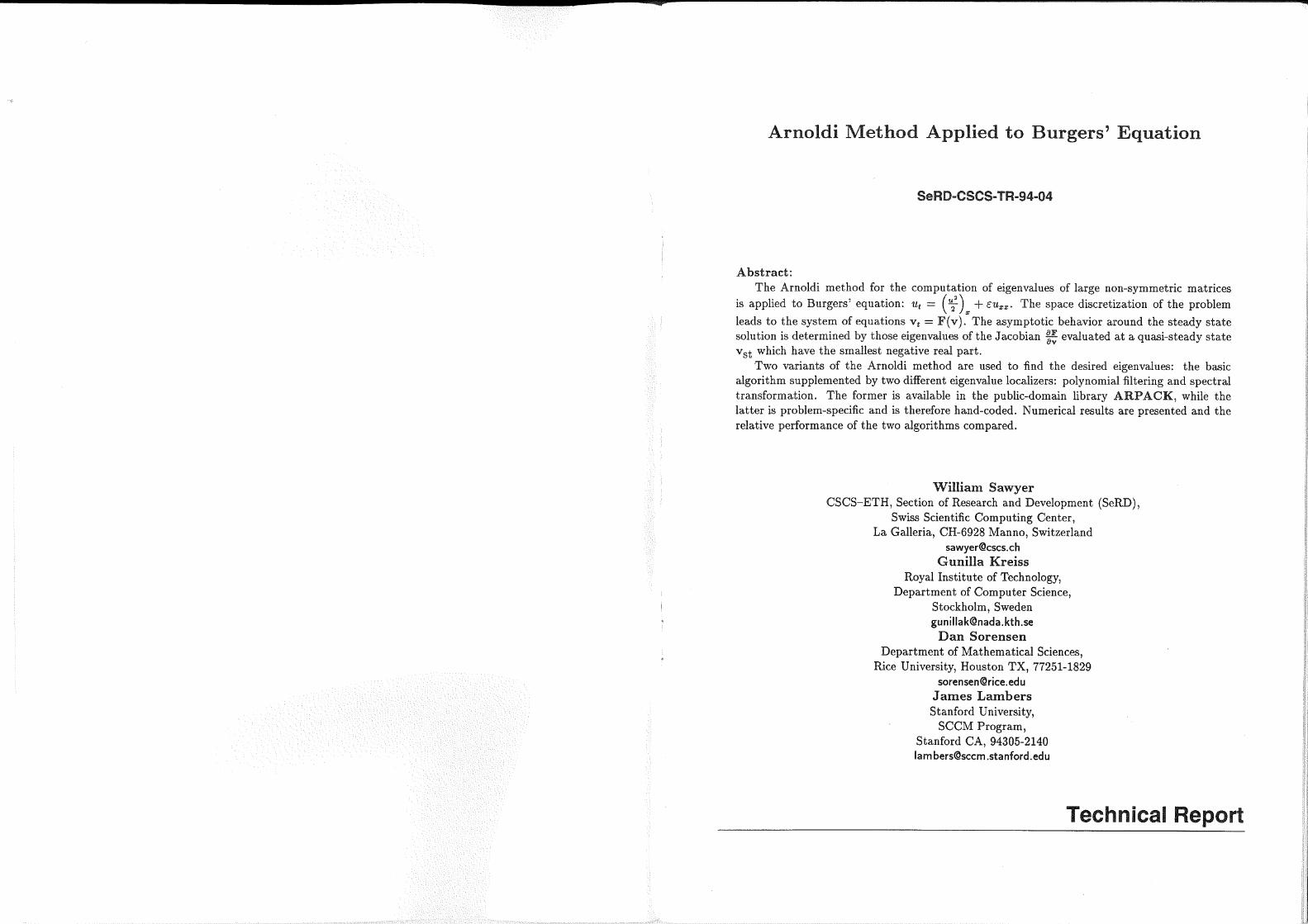
if j < n

end

hj+i,j := ft

end

4.2 Numerical Algorithms to determine the Eigenvalues of A

Both of the modified Arnold! methods share the same procedure up to the actual eigenvalue

solver:

1. Discretization; Choose the discretization by choosing h = 1/N.

2. Steady State: Find a quasi-steady state solution by using a ODE solver on equation (2)until V( is sufficiently small (i.e. its normed change in each step is less than some tolerance

tot).

3. Frechet derivative; Generate an approximation of the Jacobian at the steady state

solution found above using approximation (5). This implies deciding on the order of the

approximation as well as assigning the value of S in (18) or (19).

The evaluation of the Frechet derivative is equivalent to forming the matrix vector product

Aa;, which is required in either of the two following variations of the Arnold! method.

K-Step Arnold! Method with Polynomial Filters

Numerous problems arise in determining the eigenvalues closest to the imaginary axis using the

Arnold! method. The matrix A is large and sparse, but H will generally not be sparse. Since

the desired eigenvalues are near to the origin, they will not be the first ones found. Therefore

the plain Arnold! method's space requirements are not known a priori and are presumably large,

as is the expected amount of calculation.

Many proposals have been made to revise these deficiencies of the plain Arnoldi method.Saad in [7] has proposed an algorithm to explicitly restart the algorithm after k and usinginformation from Q to construct a new initial vector.

Sorensen in [8] proposes a related idea. First k Arnold! steps are performed. In a loop, p

more Arnold! steps are performed, then p "unwanted" eigenvalues (see below) are chosen and

filtered out using the implicit shift algorithm (see [4] for details). The matrices Hfc+p, and 'Vk+pare partitioned into an unwanted parts Hp,Vp and a desired part H^,V^. In short,

AV, =(¥„,?) AV,+=(V,+,r+)k-^k+p-l-k

Hfêl

i.e. the new equation has exactly the same form as (20), meaning that the same process can be

repeated again. This procedure has the result of implicitly restarting the algorithm with a newinitial vector v+:

v<(—^(A)v (=v+) (21)

where the ^(A) = (1/r) nî(A-^j) is the filtering polynomial (r is a normalization parameter).This "accordion" process of k — > k+p — ^ k — > k+ p- • • repeats until is /3^ < tol.

This process is not necessarily intuitive since it is not obvious that H^+p and Vfc+p can be

partitioned into a good and bad part, nor is it readily apparent that the k "good" Ritz values

12 SeRD-CSCS-TR-94-04


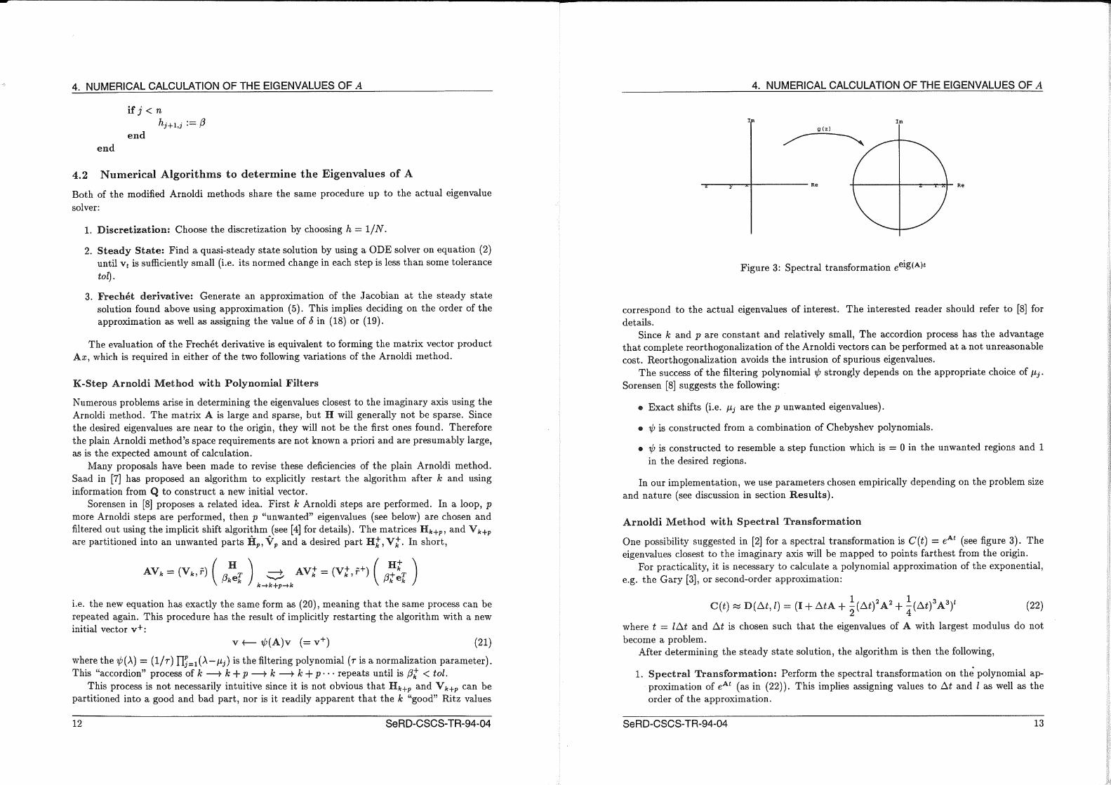
g(z)

Figure 3: Spectral transformation eel6(A)(

correspond to the actual eigenvalues of interest. The interested reader should refer to [8] for

details.

Since k and p are constant and relatively small, The accordion process has the advantage

that complete reorthogonalization of the Arnold! vectors can be performed at a not unreasonable

cost. Reorthogonalization avoids the intrusion of spurious eigenvalues.

The success of the filtering polynomial if) strongly depends on the appropriate choice of p,j .

Sorensen [8] suggests the following:

• Exact shifts (i.e. p,j are the p unwanted eigenvalues).

• ^ is constructed from a combination of Chebyshev polynomials.

• ^ is constructed to resemble a step function which is = 0 in the unwanted regions and 1

in the desired regions.

In our implementation, we use parameters chosen empirically depending on the problem size

and nature (see discussion in section Results).

Arnold! Method with Spectral Transformation

One possibility suggested in [2] for a spectral transformation is C(t) = e (see figure 3). Theeigenvalues closest to the imaginary axis will be mapped to points farthest from the origin.

For practicality, it is necessary to calculate a polynomial approximation of the exponential,

e.g. the Gary [3], or second-order approximation:

1/A*\2A2 i lfA*\3A3\lC(t) « D.(At, J) = (I + AtA + ^(At)'A2 + 7(A()-1A3) (22)

where t = lAt and At is chosen such that the eigenvalues of A with largest modulus do not

become a problem.

After determining the steady state solution, the algorithm is then the following,

1. Spectral Transformation; Perform the spectral transformation on the polynomial ap-

proximation of eAt (as in (22)). This implies assigning values to At and I as well as theorder of the approximation.



2. Arnoldi Iteration; Find the eigenvalues, hopefully with largest absolute value, by ap-

plying Arnoldi's method. These correspond to the eigenvalues of A with smallest negative

real part. We can influence this process by changing the initial vector v and varying the

number of iterations (i.e. the dimension k of the Hessenberg matrix H).

3. Reverse Transformation: Transform the eigenvalues back with eig(A) = logeig(C)/t.

Given the values of e and h it is necessary to find reasonable values for the parameters, S,

At, 1, v, fc, as well as to decide on the tolerance tol and the orders of the Frechet and Polynomial

approximations.

In order to choose At the eigenvalue of largest modulus must be considered. Keep in mind

that it is much smaller than the eigenvalues of interest. Clearly this eigenvalue would map to a

point very near the origin if we used the transformation eAt. In the polynomial approximation,

however, this eigenvalue could map to one with greater absolute value than the eigenvalues of

interest. Such an occurrence would defeat the purpose of the transformation. Consider the

simplest polynomial approximation:

,AAt 1+AtX

Amin « °

Clearly, if At >

Arnold! method wil'mm

the transform of eigenvalue A^^ will be outside the unit circle. The

tend to find that eigenvalue instead of the ones of interest.

As a general rule, we can safely set

At =Amm

in any of the of the polynomial approximations. The far left of the spectrum of A will bedominated by B in (7). It is known that,

0 > eig(B) >-4e

h2

and it is therefore safe to set,

^=£4s

(23)

A better approximation of Aj^^ can be found quickly by using a few iterations of the powermethod (see [4]).

The optimal value oft apparently varies inversely proportional to e. To make this plausible,we offer the following argument. For good convergence of the eigenvalue estimates using the

Arnoldi method, we would like,

l^'+ll

IN<.l-p

where the ;u, = eA'(A)t are the eigenvalues of the transformed system and p is not "too" small.

If k eigenvalues are needed,^k+l ^ -(A,,+i-Ak)t < ^ _

i^k

Although the distribution of the A, is not known a priori, the eigenvalues are real, negative

and range from —î to 0. Numerical experiments show that they do not bunch up as e varies.


4. NUMERiCAL CALCULATION OF THE EIGENVALUES OF A

In fact, the basic distribution stays the same while their range increases with growing epsilon.

Therefore it is safe to assume that,

Therefore,

(\k+l - Afc) ~ £

e-ket ^ 1 - p

in other words, t should be inversely proportional to e. An appropriate value for any particular

t is found by manipulating I.The value of I is a tradeoff between accuracy and efficiency: the larger I is, the larger the

separation between the eigenvalues of the transformed system near the unit circle. On the other

hand, the computational cost is increases with increasing I. It is conceivable that a smaller I

will require more Arnold! iterations before the required accuracy for the desired eigenvalue is

found.

The initial vector v also has a direct effect on fc, namely, a "good" initial vector allows for

fewer Arnold! iterations. A random vector could be used. It would be useful to have the initial

vector close to an eigenvalue of A. Such initial vector can be found be using consecutive iterates

in the determination of the pseudo-steady state. Assume that Vn and Vn-i are close to each

other and to the steady state Vg^. Then,

(v»)t = F(v»)=F(v»_i+(v»-v»_i))

0F|F(v.-,)+^ (V» - V»_i)

lv»_i

» (Vn-l)t+A(Vn-Vn_i)

(V» - V«_i)^ » A(V» - Vn_i)

Therefore, if the time steps are close enough together we are near enough to a steady state,

-^(Vn - V«_i) = A(V« - V«_i)

in other words, v = v» — Vn_i is a fair estimation of an eigenvector and thus a better choice for

the initial vector than a purely random guess.

The order of the polynomial approximation and the Frechet derivative as well as the tolerance

tol are determined such that they do not effect the accuracy of the calculations. We used the

second order Gary approximation and the fourth order Frechet derivative. The value of tol is

chosen to be 10-6.

A discussion of the proper value for S can be found in [2]. The value is chosen to be 10- .


5. NUMERICAL RESULTS

5 Numerical Results

It is possible to anticipate some of the results by analyzing the problem qualitatively.

• Consider the case h —>• 0. The matrix A will become very nearly a symmetric matrix with

constant diagonal and sub-diagonal elements with the proportion 1 : -2 : 1. This is a

well-known one-dimensional discrete Laplacian matrix with the eigenvalues,

for small i the cos i * h

A.= ^(-2+2cos(z*/i))

1 — '-y- and therefore

A..=ÂI=T

Therefore the largest eigenvalues will stay approximately constant for h very small.

Consider the case h -r 2e,e <^. 1. It is clear that t>i « v^ « 1, i.e. the shock of the steady

state solution is very "narrow." Taking (17) and insert (13) with Vi w v^ « 1 we find,

/3i-{2e-h)2

{2e+h~)2e

which goes to zero for h —>• 2e. This indicates that the corresponding A is close to singular.

Therefore we expect at least one eigenvalue to approach zero.

In general, we search for the five eigenvalues with largest real part for cases where h < 2e,

where e varies from the near shock value of 0.0125 to the very well-behaved value of 0.2. Other

cases are explored in order to analyze the effect of different parameters.

5.1 Results with Exponential Transformation

We present the results for the method discussed in section 4.2. The largest eigenvalue (nearest

to the origin) is calculated for N = 100 to N == 800. The size k of the Hessenberg matrix forthese tests is held at 25 which seems to insure that the largest eigenvalue is always found. A(

took on the value such that the eigenvalue of largest modulus, estimated by a few iterations of

the power method, is mapped by the exponential approximation to the value 0.8, avoiding its

influence among the eigenvalues of interest.

An acceptable value of * (and therefore J) is determined heuristically — at a certain point

an increase in / will not improve accuracy. A random initial vector is used in every case.

£

0.0250.05

0.1

0.2

-1

-1

-1

-9

99.32541? - 07

.7855P - 03

.3524D - 01

.570325 - 01

199

-1.5638.D

-1.8069D

-1.3536D

-9.5703D

Order

-07

-03

01-01

N399

-1.6374D-

-1.8137P.

-1.3539D-

-9.5702D -

07030101

799-1.6369D-07

-1.8154D-03

-1.3539D-01

-9.5702I? - 01

At* I

0.032

0.016

0.008

0.004

In the first place we see that the largest eigenvalue Ai is virtually independent of the step

size for all large N. In addition, note that as e

to zero, as expected.

^, the largest eigenvalue seems to converge



The results in this table are quite impressive, but there are two major deficiencies in this

method. First, backing oiF only slightly from the parameter At or trying to decrease t from the

given optimum mentioned above, yields completely erratic behavior in the eigenvalues — this

indicates the extreme sensitivity of the polynomial approximation of the exponential. Secondly,

these results are computationally extremely expensive. For the final row in the table above,

namely for e == 0.2, we find,

N= 99 199 399 799Matrix-vector multiplications

N-Vector operations

1362 1140 1095 1003545611 1061422 2101836 3342848

Even though the Arnold! method generally approximates the eigenvalues of largest modulus,

this is not guaranteed. Experimentation tells us that this is sometimes not the case. In figure 4,

the first three Ritz values are plotted against the size of the Hessenberg matrix k. As expected,

the algorithm generally approximates eigenvalues closest to the imaginary axis, i.e. the trans-

formed approximations are closest to the unit circle. However there are exceptions — some such

eigenvalues are properly approximated in later iterations, as indicated by the "jumps" in the

curves. These jumps indicate the point at which an intermediate eigenvalue starts to appear.

Note that the all the Ritz values in these test are real or nearly real.

As mentioned in the previous section, the choice of the initial vector plays a noticeable,

if not significant, role in the accuracy of the eigenvalues. For the case N == 40, e = 0.2 and

At = 0.001 and k = 5, we find the following five eigenvalue approximations for the two different

initial vectors.

Initial vector-^-

A,Ag\4As

Random

-0.9706

-8.4504

-18.2756

-59.3304

-179.4162

V« - V»_i

-0.9457

-7.4739

-17.2479

-30.9016

-63.6642

The cost of this calculation is approximately 6,500 matrix-vector multiplications. It turns

out that only the first of the values in the middle column is an accurate approximation for an

eigenvalue, while four of five in the right column are. To find similar accuracy for four eigenvalues

with a random initial vector k must be increased to 8, involving about 10,000 matrix operations.

A comparable improvement using v == v» — Vn_i is observed for other values of N and e.

5.2 Results with Filtering Polynomials

Along with the standard parameters N and £-, The tolerance for these results [s set at 0.0001.

Generally the subspace dimension r is kept below 1/10 of the size of the system (n). Thisdiffers from the previous method, where it is sufficient to keep the subspace dimension k = 25

constant.



-180

First five eigenvalues as function of Hessenberg matrix size-X-

5.5 6.5 .7 7.5 8 8.5Hessenberg matrix size

Figure 4: Five largest eigenvalues vs. size k of the Hessenberg matrix for e = 0.2. Notice the

eigenvalue "jumps" for small k.

£

0.025

0.05

0.1

0.2

99-1.54955D

-1.77973D

-1.35242D-9.57063D

-07

-03

01-01

Order

199-1.7833615-07

-1.806941?-03

-1.353581?-01

-9.57036D - 01

N399

-3.97836D -

-1.81372P.

-1.35387D-

-9.57030D -

07030101

799-4.94888D -

-1.81542D

-1.35394D-

-9.57030P-

07030101

These values compare acceptably with the those from the exponential transformation method,

although they seem to be somewhat less accurate. The very small positive values for the eigen-

values are still well within the given tolerance of 0.0001.

This algorithm is considerably more efficient than the previous one, even if one accounts for

the additional overhead involved in polynomial filtering. For the calculation of the final row inthe table (f = 0.2), the following number of matrix vector multiplications are necessary,

N=Matrix-vector multiplications

r = k +p = Number of columns of V

99 199 399 79918525

45535

124545

320555



epsilon = 0.025, N = 40,60,80,100,120, 140

8 -11.6 -11.4 -11.2 -11 -10.8 -10.6 -10.4 -10.2

Figure 5: Second and third eigenvalues as function of problem size: e = 0.025, \y (symbol: *),

As (symbol: o), depending on N.

The increase in number of matrix-vector multiplications for increasing N can be partially

offset by using a larger r = k + p (number of columns for V). Thus for N = 799, only 2735multiplications are needed for r = 70.

Not only does the largest eigenvalue, but also neighboring eigenvalues converge well. Con-

sider the second and third largest eigenvalues plotted in figure 5.

Even though all the cases treated should have purely real eigenvalues, it is possible, even

likely, that for small e numerical effects come into play which corrupt the eigenvalues. In figure 6,

six eigenvalues are found for each of five different values for N with e = 0.0125.

In each of these cases the eigenvalue with largest real part is incorrupted (it is approximately

zero). The other eigenvalues appear as complex conjugate pairs until N = 120 (using r = 20)

where the five largest eigenvalues are again entirely real.

One can see that this effect arises from numerical problems which can be avoided by in-

creasing the size of the subspace (r) to an unrealistically large size. For N = 80, r = 60 andN = 100, r = 55 all the first five eigenvalues have "settled down" and are found to be real.

Even though a pseudo steady state solution with "wiggles" does not properly represent

the true steady state, we found the largest eigenvalues for the case in figure 2. Recalling our

analytical evaluation of the problem, the stability proof relies on the absence of wiggles h < 2eas well as the proof that the eigenvalues are real.

For e = 0.001, N = 100 we find that the first three eigenvalues,

4.221 X 10- - 18.86 + 71.94? -18.86-71.94z

Even more interesting is the case e = 0.0125, N = 16: In this case, wiggles are present and



6t

4t

2\

5'|0|-

-2\

-4[

-6[

-!lo-

epsilon=0.0125for

-]—T0

Xis

0-

x

?K

+o + >t-m-

Kx "

0.

Xx

0j_.,....,_,_.__...__„ L

-25 -20

N=40,60,80, 100,1201——•-"-""•••""••-—-"""""" i- T

1

j_,, I_,,,--— L

-15 -10 -5 (

real

Figure 6: Six smallest eigenvalues as a function of problem size. Note the complex eigenvalues.

e = 0.0125, N = 40: o, 60: x, 80: *, 100: ., 120: +

there is an unmistakable positive eigenvalue.

Ai = +0.006591

There are, in addition, numerous complex eigenvalues (see Figure 7). This case serves as a

example that a pseudo-steady state with wiggles has lost the qualitative nature of the problem.

5.3 Comparisons and Conclusions

It is difficult to compare the exponential transformation and the polynomial filtering algorithms,due to their very different nature.

The number of matrix-vector multiplications is favorable for the polynomial filtering al-

gorithm for small problems. But since this operation can be computed at low cost for this

problem due to the sparsity of the matrix, most of the expense is in other parts of both algo-

rithms. While the number of floating point operations or vector operations would provide a

more useful criteria, these data are not currently available from ARPACK.

A simple comparison can be made from wall-clock time. The polynomial filtering algorithm

is consistently several times faster than the exponential transformation algorithm to obtain

the same accuracy for the same input parameters e and N, even if adjustments are made in

the transformation method to incorporate a better-than-random initial guess and the subspace

dimension k is decreased to the absolute minimum. This is still not a significant comparison,

since neither of these algorithms have been optimized.



15

10h

5h

-5h

-10|

-15,

T-

X

J_L

T"""""" •""""•""'•"'"" "••""• I•"•"•"—"—"""""""•"" T

i

s)»

x

as

x

X

SK

x)K

x

J_I_L

T—T

iK

J^ ^,-,^—— L-~14 -12 -10 -6 -4 -2

Figure 7: All eigenvalues of problem with "wiggles". N = 16, e = 0.0125

On the other hand, the polynomial filtering algorithm used in ARPACK has clearly shownits usability, since it is available in an existing library and can be utilized with ease for this prob-lem. It provides results which compare favorably with those of the exponential transformation

algorithm, which requires considerably more design and development time.


REFERENCES

References

[1] R. Lehoucq: User's Guide for ARPACK on the Touchstone Delta. Draft, netlib documen-

tation for SCALAPACK library, 1994.

[2] L. E. Eriksson and A. Rizzi: Computer-Aided Analysis of the Convergence to Steady Stateo/ Discrete Approximations to the Euler Equations. Journal of Computational Physics 57,

90-128 (1985).

[3] J. Gary: On Certain Finite Difference Schemes for Hyperbolic Systems. Math. Comp. , 18,

1 - 18 (1964).

[4] G. Golub and C. Van Loan: M'atrix Computations. Johns Hopkins University Press, Balti-

more, 1989.

[5] P. Henrici: Essentials of Numerical Analysis. Wiley and Sons, New York, 1982.

[6] ]VL Marcus and H. Mine A Survey of Matrix Theory and Matrix Inequalities. Dover Publi-

cations, New York, 1964.

[7] Y. Saad Chebyshev Acceleration Techniques for Solving Nonsymmetric Eigenvalue Prob-lems, Math. Comp., 42 (1984), pp. 567-588.

[8] D. Sorensen: Implicit Application of Polynomial Filters in a k-step Amoldi M.ethod. SIAM

J. Matrix Analysis and Appl. 13 (1), 357 - 385 (1992).


Documents

Tschnischs Hochschufs PoSi®cn!co fsderah