Tropospheric scatter

Diffraction

Line of sight

Propagation: fundamentals and models

Carol Wilson, CSIRO

Vice-Chairman ITU-R Study Group 3 & Chairman WP 3M3rd Summer School in Spectrum Management for Radio Astronomy

31 May – 4 June 2010, Tokyo

• Introduction – why propagation matters• Mechanisms of radiowave propagation and prediction methods

• Types of models• Software• Conclusion

Outline of presentation

Why does propagation matter?

• Predict levels of interference from other radio sources

• Understand variability of interference • Assess possible interference mitigation methods

• Propagation – what happens to an radio signal as it travels.

• Enough signal where you want it to be? (System design)• Too much signal where you don’t want it to be? (Interference)

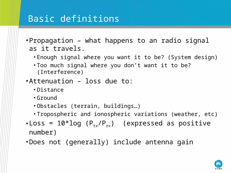
• Attenuation – loss due to:• Distance• Ground• Obstacles (terrain, buildings…)• Tropospheric and ionospheric variations (weather, etc)

• Loss = 10*log (Ptx/Prx) (expressed as positive number)

• Does not (generally) include antenna gain

Basic definitions

Mechanisms of propagation

• Free space – loss due simply to distance• Generally sets the lower bound on the loss (upper bound on

interference level)

• Mechanisms that increase loss (decrease interference)• Diffraction (including sub-path diffraction)

• Attenuation by rain (snow, etc) and atmospheric gases

• Mechanisms that decrease loss (increase interference)• Reflection/refraction (ground or atmospheric layers)

• Multipath in cluttered environments

• Atmospheric ducting

• Ionospheric sporadic-E propagation (VHF/HF)

• Rain scatter

• Environment is complex and difficult (or impossible) to define in detail uncertainty in prediction. (c.f. weather forecasting)

Interference mechanisms

Tropospheric scatter

Diffraction

Line of sight

Ducting

Reflection/refraction by elevated layers

Hydrometeor scatterLine of sight with

multipath enhancement

Long-term effects

Short-term effects

ITU-R Study Group 3 Recommendations

Study Group 3 webpage:www.itu.int/ITU-R/index.asp?category=study-groups&link=rsg3&lang=en

Recommendations:

http://www.itu.int/rec/R-REC-P/en

Go here to get three free Recommendations per year:

http://www.itu.int/publications/bookshop/how-to-buy.html#free

Updated when better methods or information is available. Use most recent version. (Rec P.526-11 rather than P.526-10)

Relation between propagation values

Field strength for a given isotropically transmitted power:

E = Pt – 20 log d + 74.8Isotropically received power for a given field strength:

Pr = E – 20 log f – 167.2Free-space basic transmission loss for a given isotropically transmitted

power and field strength:

Lbf = Pt – E + 20 log f + 167.2Power flux-density for a given field strength:

S = E – 145.8where:Pt : isotropically transmitted power (dB(W))Pr : isotropically received power (dB(W))E : electric field strength (dB(V/m))f : frequency (GHz)d : radio path length (km)Lbf : free-space basic transmission loss (dB)S : power flux-density (dB(W/m2)).

From ITU-R Recommendation P.525

Free space loss

Attenuation of signal due to distance alone.

Lbf = 20 log (4d / ) dB

or in practical units

Lbf = 32.4 + 20 log(f) + 20 log (d) dB

where f is in MHz and d is in distance

For most practical situations, free space loss is the minimum loss worst case interference.

Applicable to interference from aircraft, satellites.

Apparent “line-of-sight” paths not necessarily free space loss only!

ITU-R Recommendation P.525

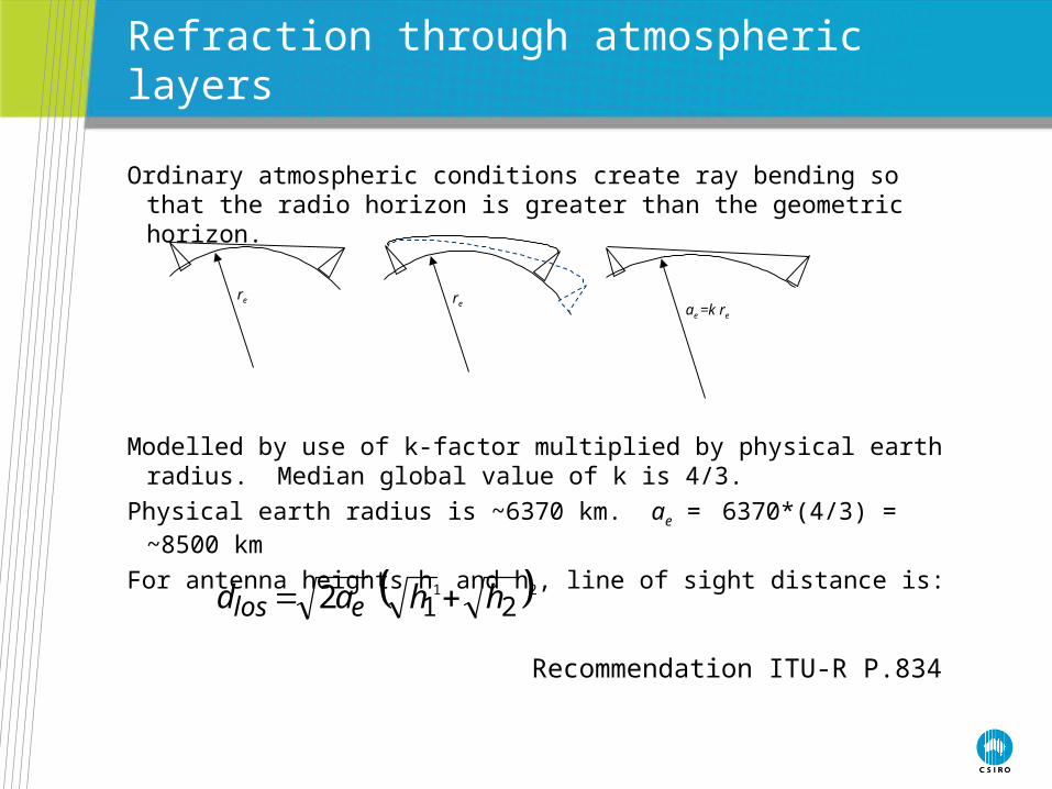
Refraction through atmospheric layers

Ordinary atmospheric conditions create ray bending so that the radio horizon is greater than the geometric horizon.

Modelled by use of k-factor multiplied by physical earth radius. Median global value of k is 4/3.

Physical earth radius is ~6370 km. ae = 6370*(4/3) = ~8500 km

For antenna heights h1 and h2, line of sight distance is:

212 hhad elos

Recommendation ITU-R P.834

reae =k re

re

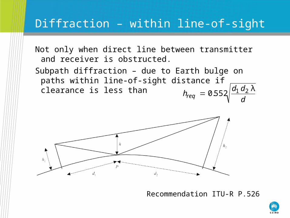
Diffraction – within line-of-sight

Not only when direct line between transmitter and receiver is obstructed.

Subpath diffraction – due to Earth bulge on paths within line-of-sight distance if clearance is less than

d

ddhreq

λ552.0 21

Recommendation ITU-R P.526

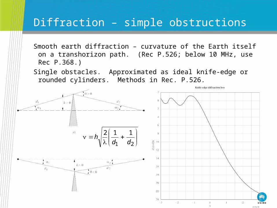
Diffraction – simple obstructions

Smooth earth diffraction – curvature of the Earth itself on a transhorizon path. (Rec P.526; below 10 MHz, use Rec P.368.)

Single obstacles. Approximated as ideal knife-edge or rounded cylinders. Methods in Rec. P.526.

21

112

ddh

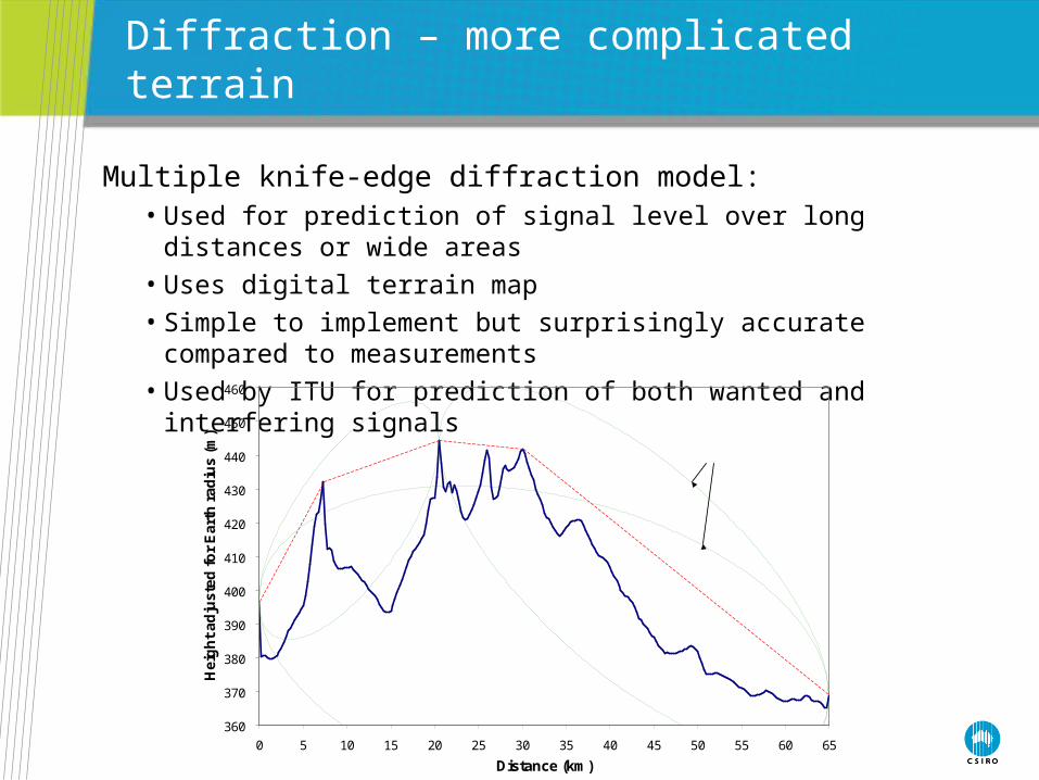
Diffraction – more complicated terrain

Multiple knife-edge diffraction model:• Used for prediction of signal level over long distances or wide areas

• Uses digital terrain map

• Simple to implement but surprisingly accurate compared to measurements

• Used by ITU for prediction of both wanted and interfering signals

360

370

380

390

400

410

420

430

440

450

460

0 5 10 15 20 25 30 35 40 45 50 55 60 65

Distance (km)

Hei

gh

t ad

jus

ted

fo

r E

arth

rad

ius

(m)

Fresnel zones

Knife-edge diffraction model

• Terrain profile includes earth curvature and atmospheric refraction

• Diffraction parameter is a function of how far the terrain point obstructs the first Fresnel zone radius:

• Point with largest on entire path: principal edge

• Points with largest either side of principal edge: auxiliary edges

• Sum diffraction loss from three edges

L  =  J(p) + {1.0 – exp( –J(p) / 6 )} [J(t) + J(r) + 10.0 + 0.04D ]

nbanabn dddh /2

dB1.0–1)1.0–(log209.6)( 2

J

Recommendation ITU-R P.526

Tropospheric scatter and ducting

• Scattering from inhomogeneities (troposcatter) is the main long-term effect on long paths (more than ~100 km) when diffraction loss becomes high.

• Ducting may occur for short periods of time due to atmospheric layers near the surface (over water or flat coastal areas) or elevated layers in the atmosphere. May be significant for distances up to ~ 300 km.

• Recommendation ITU-R P.452 gives an empirical calculation method for troposcatter, ducting and reflection from atmospheric layers.

• Scatter from rain can also calculated using Recommendation ITU-R P.452. (May be significant above ~ 5 GHz)

Mechanisms affecting HF and VHF

• Small but intense ionization layers in the E-region of the ionosphere (Sporadic-E) can cause abnormal VHF propagation for periods lasting several hours. Effect decreases with increasing frequency but can be significant up to ~135 MHz.

• Recommendation P.534 gives a method for predicting field strength and probability of occurrence.

• At frequencies to ~30 MHz, ground wave propagation is the major propagation mechanism.

• Recommendation P.368 gives a method for predicting ground wave field strength, based on curves.

Ground wave 10 kHz to 30 MHz

Other propagation mechanisms

• Multipath – reflections from objects may cause distortion of wanted signal. In some specific scenarios, may increase interference power.

• Attenuation due to rain, clouds, fog, snow, etc. Noticeable above about 5 GHz. Decreases wanted signal (and interference signal). Raises noise temperature.

• Atmospheric attenuation noticeable with increasing frequency and at specific molecular resonance frequencies. Provides good isolation between active transmitters and passive services in frequency bands above ~ 200 GHz.

Specific attenuation due to atmosphere

Chart shows specific attenuation at 1013 hPa, 15°C, water vapour density 7.5 g/m3

At frequencies above 100 GHz, loss becomes significant.

Helpful in protecting passive services as very high bands.

Types of models

• Propagation models typically used to define worst case scenario for the intended purpose.

• Interference varies with changing conditions, leading to statistical descriptions.

• Models for system design focus on high attenuation scenarios.• Models for interference focus on low attenuation scenarios.• Be cautious about applying system design propagation models

for interference analysis.

• Model accuracy depends on quality of information available.• Generic models useful when specific sites not known. • Site-specific models useful when terrain information is

available.

Key ITU-R Recommendations

Recommendation ITU-R P.452 (Prediction of interference between stations on the surface of the Earth at frequencies above 0.1 GHz)

• Uses multiple knife-edge diffraction model for specific terrain, and troposcatter, ducting, etc.

Recommendation ITU-R P.1546 (Point-to-area predictions for terrestrial services 30 MHz to 3 000 MHz). Generic terrain assumptions.

• Based on curves of measured data over a number of land paths.

• Used in 2006 by ITU as technical basis to replan broadcasting across Europe, Africa and the Middle East.

Recommendation P.1546 for 30 MHz to 3 GHz

• Curves represent field strength exceeded at 50% of locations for 1kW ERP transmission as function of:

• Frequency: 100, 600, 2000 MHz• Time: 50%, 10%, 1% • Tx antenna height: 10 to 1200 m; Rx

antenna height: local clutter height (minimum 10 m)

• Path type: land, warm sea, cold sea• Distance: 1 to 1000 km• Interpolation method for all of above.

• Curves are based on extensive measurement campaigns in Europe, North America, the North Sea and Mediterranean.

A word about software packages

• Many commercial software packages available and useful, but:

• Be aware of purpose (system design vs interference analysis)• Sometimes mistakes in coding go unnoticed.• Often out-of-date with respect to ITU-R Recommendations.• Understand the underlying mechanisms being modelled and

look for anomalies.

• ITU Study Group 3 website has some free software available on “as is” basis. (Including Rec P.452, curves for P.1546, etc)

Expectations

Propagation prediction method

Measurements “Reality”

Error:•Mean•Std Dev

???

• Prediction method development – aim to minimize mean error• Site specific models – std deviation of several dB• SG 3 goals: 1) accuracy, 2) clarity, 3) simplicity, 4) physical

representation.• On all but shortest paths, propagation loss varies with time.• Models useful for comparison of different options, for overall

statistics.• An accepted, transparent model often useful in regulatory

situations.

Conclusions

• Propagation prediction methods necessary to estimate, understand interference to radioastronomy.

• Prediction methods available from ITU (and other sources) to model various propagation mechanisms.

• Statistics of interference and system design are different.• General knowledge of propagation phenomena useful in

radioastronomy design and operation.

• See you at the Study Group 3 website!

www.itu.int/ITU-R/index.asp?category=study-groups&link=rsg3&lang=en

Contact UsPhone: 1300 363 400 or +61 3 9545 2176

Email: enquiries@csiro.au Web: www.csiro.au

Thank you!

Questions?

Carol Wilson, Research Consultantcarol.wilson@csiro.au