Freezing of living cells 1

Freezing of living cells: mathematical models and design of optimal cooling

protocols

K.-H.Hoffmann, N.D.Botkin, V.L.Turova

Abstract

Two injuring effects of cryopreservation of living cells are under study. First,stresses arising due to non-simultaneous freezing of water inside and outside of thecell are modeled and controlled. Second, dehydration of cells caused by earlier icebuilding in the extracellular liquid comparing to the intracellular one is simulated.

A low-dimensional mathematical model of competitive ice formation inside andoutside of living cells during freezing is obtained by applying an appropriate averagingtechnique to partial differential equations describing the dynamics of water-ice phasetransitions. This reduces spatially distributed relations to a few ordinary differentialequations with control parameters and uncertainties. Such equations together with anobjective functional that expresses the difference between the amount of ice inside andoutside of a cell are considered as a differential game where the aim of the control isto minimize the objective functional, and the aim of the disturbance is opposite. Astable finite-difference scheme for computing the value function is applied to the prob-lem. On the base of the computed value function, optimal cooling protocols ensuringsimultaneous freezing of water inside and outside of living cells are designed. Such aregime provides balancing the pressures inside and outside of cells, which prevents cellsfrom injuring.

Another mathematical model describes shrinkage and swelling of cells caused bytheir osmotic dehydration and rehydration during freezing and thawing. The modelis based on the theory of ice formation in porous media and Stefan type conditionsdescribing the osmotic outflow/inflow related to the change of salt concentration inthe extracellular liquid. The cell shape is searched as the level set of a function whichsatisfies a Hamilton-Jacobi equation resulting from a Stefan-type condition for thenormal velocity of the cell boundary. The arising Hamilton-Jacobi equations are treatednumerically using both a finite-difference scheme for finding viscosity solutions andthe computation of reachable sets of an associated conflict control problem. Shapeevolutions computed are presented in two and three dimensional cases.

Introduction

Our intention “Optimal control in cryopreservation of cells and tissues” is devoted to theapplication of optimal control theory to the minimization of damaging effects of cooling andthawing in order to increase the survival rate of frozen and subsequently thawed out cells.The main objective of the intention is the development of hierarchical coupled mathematicalmodels that describe the most injuring effects of cryopreservation of living cells and especiallytissues. The central point of the previous work was the development of optimized coolingprotocols that minimize damaging effects of freezing related to the release of the latent heatand irregular ice formation. A detailed description of these topics can be found in [10], [11].This paper continues the work and considers two most damaging factors of cryopreservation:large stresses exerted on cell membranes and dehydration/rehydration effects.

The main of injuring factors is a large stress exerted on cell membranes. It occurs atslow cooling because of non-simultaneous freezing of extracellular and intracellular fluids.The use of rapid cooling rates is not a perfect solution because water inside cells formssmall, irregularly-shaped ice crystals (dendrites) that are relatively unstable. If frozen cells

2 K.-H.Hoffmann, N.D.Botkin, V. L.Turova

are subsequently thawed out, dendrites will aggregate to form larger, more stable crystalsthat may cause damage. Therefore, it is reasonable to apply control theory to providesimultaneous freezing of extracellular and intracellular fluids even for slow cooling rates.Therefore, a mathematical model describing freezing and thawing is to be formulated alongwith optimization criteria. Note that models of phase transitions are basically utilize par-tial differential equations that describe the dynamics of phases in each spatial point (seee.g. [4], [8], [9]). Nevertheless, the spatial distribution is not very important, if small objectssuch as living cells and pores of the extracellular matrix are investigated. Our experienceshows that appropriate averaging techniques accurately reduce spatially distributed modelsto a few ordinary differential equations with control parameters and uncertainties. However,such equations contain as a rule nonlinear dependencies given by tabular data. Thus, theuncertainties and non-smooth nonlinearities complicate the application of traditional controldesign methods based on Pontryagin’s maximum principle. Nevertheless, the dynamical pro-gramming principle related to Hamilton-Jacobi-Bellman-Isaacs (HJBI) equations is suitable,if stable grid methods for solving HJBI are available. This paper considers a stable gridprocedure that allows us to design optimized controls (cooling protocols) for an ODE systemdescribing competitive ice formation inside and outside of living cells.

The second injuring factor studied in this paper is excessive shrinkage and swelling of cellsdue to the osmotic dehydration and rehydration occurring in freezing and warming phases,respectively. The paper considers mathematical models of these effects caused by the osmoticpressure arising due to different salt concentrations in the extracellular and intracellularliquids. Conventional models of cell dehydration during freezing (see e.g. [1], [14]) describethe change of the cell volume depending on mass diffusion, heat transfer, and the evolutionof the freezing front. The cell shape is supposed to be spherical or cylindrical. However,as it is reported by biologists (see e.g. [5]), keeping both the cell size and shape is veryimportant for cell survival. Mathematical models proposed in this paper are concerned withthe evolution of the cell shape depending on the temperature distribution and the amountof the frozen liquid outside the cell. The models are based on the theory of ice formationin porous media developed in [8] and Stefan type models [4] describing the osmotic outflow(inflow) caused by the increase (decrease) of salt concentration in the extracellular liquidduring its freezing (thawing). The resulting model equations of the Hamilton-Jacobi typeare treated numerically using both a finite-difference scheme for finding viscosity solutionsand the computation of reachable sets of an associated conflict control problem formalizedaccording to [15, 17]. The computed shape evolutions are presented.

1. Mathematical model of ice formation

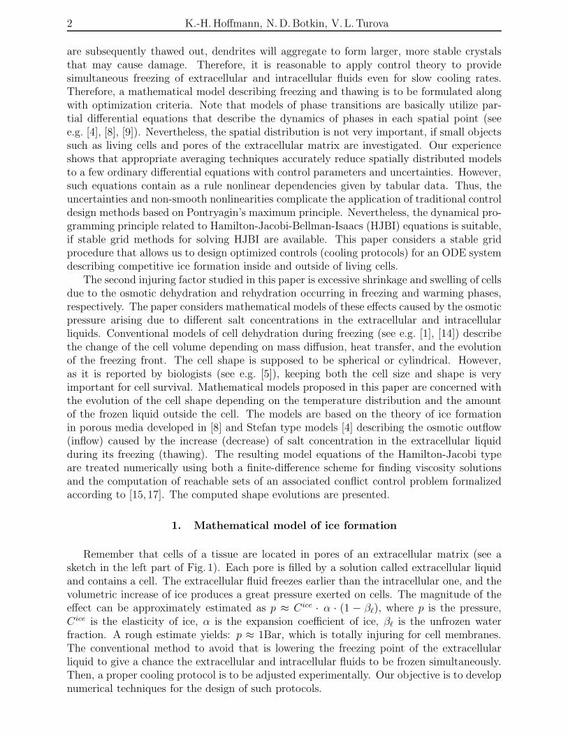
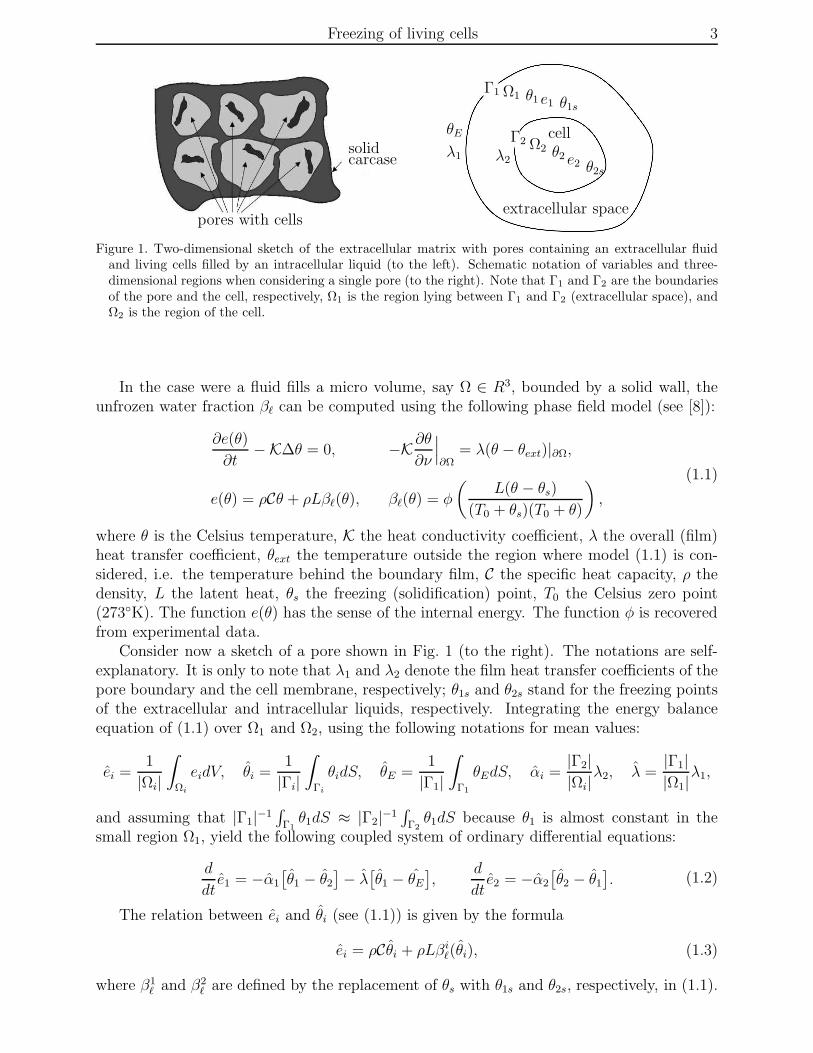
Remember that cells of a tissue are located in pores of an extracellular matrix (see asketch in the left part of Fig. 1). Each pore is filled by a solution called extracellular liquidand contains a cell. The extracellular fluid freezes earlier than the intracellular one, and thevolumetric increase of ice produces a great pressure exerted on cells. The magnitude of theeffect can be approximately estimated as p ≈ Cice · α · (1 − βℓ), where p is the pressure,Cice is the elasticity of ice, α is the expansion coefficient of ice, βℓ is the unfrozen waterfraction. A rough estimate yields: p ≈ 1Bar, which is totally injuring for cell membranes.The conventional method to avoid that is lowering the freezing point of the extracellularliquid to give a chance the extracellular and intracellular fluids to be frozen simultaneously.Then, a proper cooling protocol is to be adjusted experimentally. Our objective is to developnumerical techniques for the design of such protocols.

Freezing of living cells 3

pores with cells

solidcarcase

Γ1 Ω1 θ1 e1 θ1s

extracellular space

cellΓ2 Ω2 θ2 e2 θ2s

θE

λ1 λ2

Figure 1. Two-dimensional sketch of the extracellular matrix with pores containing an extracellular fluidand living cells filled by an intracellular liquid (to the left). Schematic notation of variables and three-dimensional regions when considering a single pore (to the right). Note that Γ1 and Γ2 are the boundariesof the pore and the cell, respectively, Ω1 is the region lying between Γ1 and Γ2 (extracellular space), andΩ2 is the region of the cell.

In the case were a fluid fills a micro volume, say Ω ∈ R3, bounded by a solid wall, theunfrozen water fraction βℓ can be computed using the following phase field model (see [8]):

∂e(θ)

∂t−K∆θ = 0, −K∂θ

∂ν

∣

∣

∣

∂Ω= λ(θ − θext)|∂Ω,

e(θ) = ρCθ + ρLβℓ(θ), βℓ(θ) = φ

(

L(θ − θs)

(T0 + θs)(T0 + θ)

)

,

(1.1)

where θ is the Celsius temperature, K the heat conductivity coefficient, λ the overall (film)heat transfer coefficient, θext the temperature outside the region where model (1.1) is con-sidered, i.e. the temperature behind the boundary film, C the specific heat capacity, ρ thedensity, L the latent heat, θs the freezing (solidification) point, T0 the Celsius zero point(273K). The function e(θ) has the sense of the internal energy. The function φ is recoveredfrom experimental data.

Consider now a sketch of a pore shown in Fig. 1 (to the right). The notations are self-explanatory. It is only to note that λ1 and λ2 denote the film heat transfer coefficients of thepore boundary and the cell membrane, respectively; θ1s and θ2s stand for the freezing pointsof the extracellular and intracellular liquids, respectively. Integrating the energy balanceequation of (1.1) over Ω1 and Ω2, using the following notations for mean values:

ei =1

|Ωi|

∫

Ωi

eidV, θi =1

|Γi|

∫

Γi

θidS, θE =1

|Γ1|

∫

Γ1

θEdS, αi =|Γ2||Ωi|

λ2, λ =|Γ1||Ω1|

λ1,

and assuming that |Γ1|−1∫

Γ1

θ1dS ≈ |Γ2|−1∫

Γ2

θ1dS because θ1 is almost constant in thesmall region Ω1, yield the following coupled system of ordinary differential equations:

d

dte1 = −α1

[

θ1 − θ2

]

− λ[

θ1 − θE

]

,d

dte2 = −α2

[

θ2 − θ1

]

. (1.2)

The relation between ei and θi (see (1.1)) is given by the formula

ei = ρCθi + ρLβiℓ(θi), (1.3)

where β1ℓ and β2

ℓ are defined by the replacement of θs with θ1s and θ2s, respectively, in (1.1).

4 K.-H.Hoffmann, N.D.Botkin, V. L.Turova

-15 -10 -5 0 5 100

0.2

0.4

0.6

0.8

1

θ

βℓ(θ)

e

θ

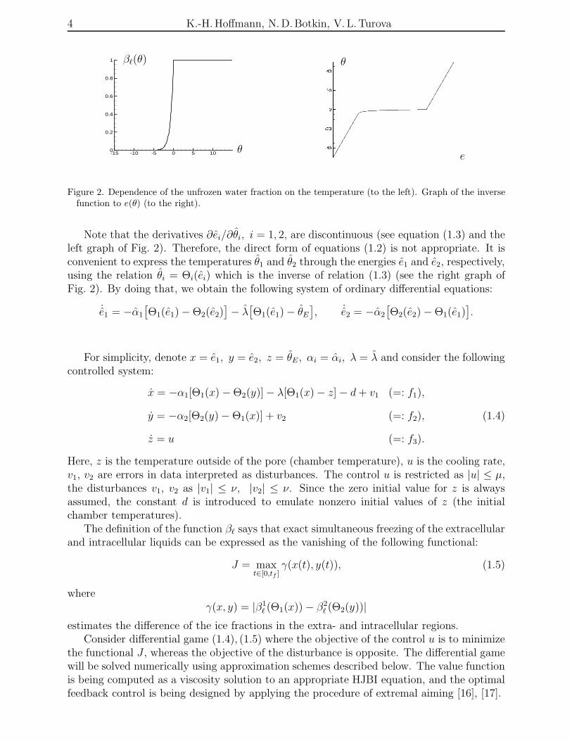
Figure 2. Dependence of the unfrozen water fraction on the temperature (to the left). Graph of the inversefunction to e(θ) (to the right).

Note that the derivatives ∂ei/∂θi, i = 1, 2, are discontinuous (see equation (1.3) and theleft graph of Fig. 2). Therefore, the direct form of equations (1.2) is not appropriate. It isconvenient to express the temperatures θ1 and θ2 through the energies e1 and e2, respectively,using the relation θi = Θi(ei) which is the inverse of relation (1.3) (see the right graph ofFig. 2). By doing that, we obtain the following system of ordinary differential equations:

˙e1 = −α1

[

Θ1(e1) − Θ2(e2)]

− λ[

Θ1(e1) − θE

]

, ˙e2 = −α2

[

Θ2(e2) − Θ1(e1)]

.

For simplicity, denote x = e1, y = e2, z = θE , αi = αi, λ = λ and consider the followingcontrolled system:

x = −α1[Θ1(x) − Θ2(y)] − λ[Θ1(x) − z] − d + v1 (=: f1),

y = −α2[Θ2(y) − Θ1(x)] + v2 (=: f2),

z = u (=: f3).

(1.4)

Here, z is the temperature outside of the pore (chamber temperature), u is the cooling rate,v1, v2 are errors in data interpreted as disturbances. The control u is restricted as |u| ≤ µ,the disturbances v1, v2 as |v1| ≤ ν, |v2| ≤ ν. Since the zero initial value for z is alwaysassumed, the constant d is introduced to emulate nonzero initial values of z (the initialchamber temperatures).

The definition of the function βℓ says that exact simultaneous freezing of the extracellularand intracellular liquids can be expressed as the vanishing of the following functional:

J = maxt∈[0,tf ]

γ(x(t), y(t)), (1.5)

whereγ(x, y) = |β1

ℓ (Θ1(x)) − β2ℓ (Θ2(y))|

estimates the difference of the ice fractions in the extra- and intracellular regions.Consider differential game (1.4), (1.5) where the objective of the control u is to minimize

the functional J , whereas the objective of the disturbance is opposite. The differential gamewill be solved numerically using approximation schemes described below. The value functionis being computed as a viscosity solution to an appropriate HJBI equation, and the optimalfeedback control is being designed by applying the procedure of extremal aiming [16], [17].

Freezing of living cells 5

2. Hamilton-Jacobi-Bellman-Isaacs equations

The game (1.4), (1.5) is formalized as in [16], [17], and [20] so that the value function Vexists. The next important result proved in [21] says that V coincides with a unique viscositysolution (see [6], [7], and [2]) of the following HJBI equation:

Vt + H(x, y, z, Vx, Vy, Vz) = 0, (2.6)

where the Hamiltonian H and the majoration and terminal conditions are defined as

H(x, y, z, p1, p2, p3) = max|v1|,|v2|≤ν

min|u|≤µ

3∑

i=1

pifi, V (t, x, y, z) ≥ γ(x, y), V (tf , x, y, z) = γ(x, y).

In the next section, an approximation scheme for solving this HJBI equation is discussedand convergence results are given.

3. Approximation schemes and convergence results

Let τ, ∆x, ∆y, ∆z be time and space discretization step sizes. Introduce the followingnotation:

V n(xi, yj, zk) = V (nτ, i∆x, j∆y, k∆z), N τ = tf

and consider a difference scheme:

V n−1(xi, yj, zk) = V n(xi, yj, zk) + τH(xi, yj, zk, Vnx , V n

y , V nz ), V N (xi, yj, zk) = γ(xi, yj).

Here, the symbols V nx , V n

y , V nz denote finite difference approximations (left, right, central

and etc.) of the corresponding partial derivatives. The scheme can be considered as theapplication of an operator Π to the grid function V n to obtain V n−1:

V n−1 = Π(V n; τ, ∆x, ∆y, ∆z).

It is clear that such an operator can be naturally extended to continuum functions.

Definition 1. The operator Π is monotone, if the following implication holds:

V ≤ W ⇒ Π(V ; τ, ∆x, ∆y, ∆z) ≤ Π(W ; τ, ∆x, ∆y, ∆z),

where the point-wise order is assumed.

Definition 2. The operator Π has the generator property, if the following estimateholds:

∣

∣

∣

∣

Π(φ; τ, aτ, bτ, cτ)(~r) − φ(~r)

τ− H(~r, Dφ(~r))

∣

∣

∣

∣

≤ C(

1 + ‖Dφ‖ + ‖D2φ‖)

τ (3.7)

for every φ ∈ C2b (R3), ~r = (x, y, z) ∈ R3, and fixed a, b, c > 0. Here C2

b (R3) is the space of

twice continuously differentiable functions defined on R3 and bounded together with theirtwo derivatives, ‖ · ‖ denotes the point-wise maximum norm, Dφ and D2φ denote the gradi-ent and the Hessian matrix of φ.

6 K.-H.Hoffmann, N.D.Botkin, V. L.Turova

Theorem 1. (convergence, [2], [19]). Assume that the operator Π(·; τ, aτ, bτ, cτ) is mono-tone for any τ > 0 and satisfies the generator property, then the grid function obtained bythe procedure:

V n−1 = maxΠ(V n; τ, aτ, bτ, cτ), γ, V N = γ, (3.8)

converges point-wise to a unique viscosity solution of (8.13) and, therefore, to the valuefunction of the differential game (1.4), (1.5) as τ → 0. The convergence rate is

√τ .

Remark 1. Theorem 1 refer only to the monotonicity and generator properties of theoperator Π. Really, some secondary properties must be held to provide the convergence(see [2] and [19]). We omit here the discussion of them because they obviously hold for anoperator Π that will be considered further.

The next section presents an upwind operator Π with the monotonicity and generatorproperties. Denote

pR1 = [V n(xi+1, yj, zk) − V n(xi, yj, zk]/∆x, pL

1 = [V n(xi, yj, zk) − V n(xi−1, yj, zk]/∆x,

pR2 = [V n(xi, yj+1, zk) − V n(xi, yj, zk]/∆y, pL

2 = [V n(xi, yj, zk) − V n(xi, yj−1, zk]/∆y,

pR3 = [V n(xi, yj, zk+1) − V n(xi, yj, zk]/∆z, pL

3 = [V n(xi, yj, zk) − V n(xi, yj, zk−1]/∆z.

4. Upwind solution operator

We will consider a solution operator proposed in [13] and prove that it is monotoneand possesses the generator property, which proves convergence claims. Unfortunately, theconvergence arguments given in [13] are very sketchy and not strong. They are solely basedon topological considerations and do not take into account the nature of viscosity solutions sothat they have little force. Nevertheless, the idea of the operator proposed there is brilliant.

Assume that the right-hand-sides fi, i = 1, 2, 3, are now arbitrary functions of the state(x, y, z), control u ∈ P ⊂ Rp, and disturbance v ∈ Q ⊂ Rq. Denote a+ = max (a, 0), a− =min (a, 0). The operator introduced in [13] assumes the following approximations of thespatial derivatives:

V nx · f1 = pR

1 · f+1 + pL

1 · f−1 , V n

y · f2 = pR2 · f+

2 + pL2 · f−

2 , V nz · f3 = pR

3 · f+3 + pL

3 · f−3 ,

where f1, f2, f3 are computed at (xi, yj, zk); pR1 , pR

2 , pR3 and pL

1 , pL2 , pL

3 the right and leftdivided differences, respectively. Finally, the operator is given by

Π(V n; τ, ∆x, ∆y, ∆z)(xi, yj, zk) = V n(xi, yj, zk) +

+τ maxv∈Q

minu∈P

(

pR1 · f+

1 + pL1 · f−

1 + pR2 · f+

2 + pL2 · f−

2 + pR3 · f+

3 + pL3 · f−

3

)

.(4.9)

Lemma 1. (monotonicity and generator property, [3]). Let M be the bound of the righthand side of the controlled system. If a, b, c ≥ M

√3, then the operator Π(·; τ, aτ, bτ, cτ) given

by (4.9) is monotone. The generator property (3.7) holds for any fixed a, b, c.

The proof is the same as in Lemmas 2 and 3 (see Section 8). Thus, the operator (4.9) satisfiesthe conditions of Theorem 1.

Remark 2. If the functions fi, i = 1, 2, 3, are linear in u and v at each fixed state(x, y, z), then the operation maxv∈Q minu∈P in the definitions of the operator (4.9) can be

Freezing of living cells 7

replaced by maxv∈ extQ minu∈extP , where “ext” returns the set of the extremal points. Inparticular, “max min” can be computed over the set of vertices, if P and Q are polyhedrons.The monotonicity holds independently of the structure of the sets P and Q. To prove thegenerator property, it is sufficient to observe that the Hamiltonian is equal to that computedusing the sets ext P and ext Q whenever the assumption of linearity in u and v at each fixedstate vector holds. Note that this remark is very important for numerical implementations ofthe operator (4.9) because the operation “max min” is applied to a function that is nonlinearand not convex/concave in u and v.

5. Control procedure

In this section, the computation of optimal controls for system (1.4) in accordance withthe procedure of extremal aiming (see [16] and [17]) is described.

Let ε be a small positive number, and tn the current time instant. Consider the neigh-borhood

Uε = (x, y, z) ∈ R3 : |x − x(tn)| ≤ ε, |y − y(tn)| ≤ ε, |z − z(tn)| ≤ ε

of the current state(

x(tn), y(tn), z(tn))

of system (1.4). By searching through all grid points(xi, yj, zk) ∈ Uε, find a point (xi∗ , yj∗, zk∗

) such that

V n(xi∗ , yj∗, zk∗) = min

(xi,yj ,zk)∈Uε

V n(xi, yj, zk).

The current control u(tn) which is supposed to be applied on the next time interval [tn, tn+τ ]is computed from the condition of maximal projection of the system velocity (f1, f2, f3) ontothe direction of the vector

(

xi∗ − x(tn), yi∗ − y(tn), zi∗ − z(tn))

, i.e.

u(tn) = argmax|u|≤µ

(

(

xi∗ − x(tn))

f1 +(

yi∗ − y(tn))

f2 +(

zi∗ − z(tn))

f3

)

.

It is clear that the value of the control will be either µ or −µ.

6. Simulation results

Let us first consider the following two-dimensional variant of the controlled system:

x = −α1[Θ1(x) − Θ2(y)] − λ[Θ1(x) − u] − d + v1

y = −α2[Θ2(y) − Θ1(x)] + v2,(6.10)

which corresponds to the assumption z ≡ u (infinite cooling rate). The values of the coeffi-cients and bounds on the control and disturbances used for all simulations are: α1 = α2 = 0.1,λ = 2, d = 2, µ = 4, ν = 0.2. The notation βi

ι := 1−βiℓ, i = 1, 2, is used for the ice fractions.

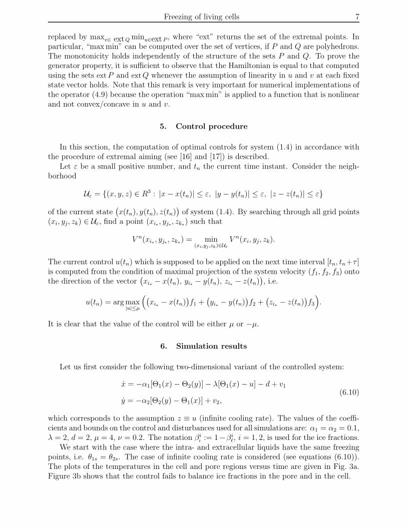
We start with the case where the intra- and extracellular liquids have the same freezingpoints, i.e. θ1s = θ2s. The case of infinite cooling rate is considered (see equations (6.10)).The plots of the temperatures in the cell and pore regions versus time are given in Fig. 3a.Figure 3b shows that the control fails to balance ice fractions in the pore and in the cell.

8 K.-H.Hoffmann, N.D.Botkin, V. L.Turova

-160

-140

-120

-100

-80

-60

-40

-20

0

20

0 2 4 6 8 10 12 14 16 18 20

(a) Temperatures in the extracellularspace and in the cell versus time;latent heat plateaus are present

0

0.2

0.4

0.6

0.8

1

0 2 4 6 8 10 12 14 16 18 20

(b) Ice fraction in the extracellularspace and in the cell versus time

β1ι (t) β2

ι (t)θ1(t)

θ2(t)

Figure 3. The case of infinite cooling rate, θ1s = θ2s.

The next simulation (see Fig. 4) shows the case of different freezing points for the poreand the cell: θ1s −θ2s = −13C. Thus, the freezing point of the extracellular fluid is lowered,e.g. by adding a cryoprotector. Now, we can freeze the intracellular fluid using temperatureslaying above the freezing point of the extracellular liquid, which makes simultaneous freezingprincipally possible. Figure 5 stands for the same setting but in the case of finite coolingrate (see equations (1.4)).

Remember that the central point of the control design is the computation of the valuefunction using the upwind grid method given by (3.8) and (4.9). Numerical experimentsshow a very nice property of this method: the noise usually coming from the boundary ofthe grid region is absent. The examples are calculated on a Linux computer admitting 64gb

memory and 32 threads. The coefficient of the parallelization is equal to 0.7 per thread (23times totally). The grid size in three dimensions is 3003, the number of time steps is 30000(see the restrictive relation between the space and time step sizes given by Lemma 1). Therun time is approximately 60 min. In the case of two dimensions the run time is severalminutes.

Freezing of living cells 9

-160

-140

-120

-100

-80

-60

-40

-20

0

20

0 10 20 30 40 50 60 70

0

0.2

0.4

0.6

0.8

1

0 10 20 30 40 50 60 70-4

-3

-2

-1

0

1

2

3

4

0 10 20 30 40 50 60 70

(a) Graph of the value function at t = 0

(b) Temperatures in the extracellularspace and in the cell versus time;latent heat plateaus are present

(c) Ice fractions in the extracellularspace and in the cell versus time

(d) Realization of the control

β1ι (t)

β2ι (t)

θ2(t)

θ1(t)

u(t)

V (0, x, y)

x0, y0

Figure 4. The case of infinite cooling rate, θ1s − θ2s = −13C.

0

0.2

0.4

0.6

0.8

1

0 10 20 30 40 50 60 70 80

(a) Graph of the value function at t = 0, z = 0 (b) Ice fractions in the extracellularspace and in the cell versus time

β1ι (t)

β2ι (t)

V (0, x, y, z)|z=0

x0, y0

Figure 5. The realistic case of finite cooling rate (three dimensions), θ1s − θ2s = −13C.

10 K.-H.Hoffmann, N.D.Botkin, V. L.Turova

7. Mathematical models of dehydration and rehydration of cells

Each biological tissue cell is located inside a pore filled with a saline solution calledextracellular fluid. The cell interior is separated from the pore by a cell membrane whosestructure ensures a very low heat conductivity but a very good permeability for water,which makes possible its easy inflow and outflow so that the osmotic pressure caused by thedifference of salt concentrations inside and outside the cell easily results in water transportinto/out of the cell.

7.1. Dehydration of cells

In the freezing phase, the mechanism of the osmotic effect is the following. Ice formationgoes initially in the extracellular solution. Since ice is practically free of salt, the waterto ice phase transition results in the increase of salt concentration (cout) in the remainingextracellular liquid. The osmotic pressure forces the outflow of water from the cell to balancethe intracellular (cin) and extracellular salt concentrations. Modeling the cell shrinkage isbased on free boundary problem techniques. The main relation here is the so called Stefancondition: Vn = α(cout − cin), where Vn is the normal velocity of the cell boundary (directedto the cell interior), and the right-hand-side represents the osmotic flux that is proportionalto the difference of the concentrations. The coefficient α is the product of the Boltzmannconstant, the temperature, and the hydraulic conductivity of the membrane (see e.g. [14]).Note that α is practically a constant in our case. The extracellular salt concentration cout

depends on the unfrozen fraction βℓ of the extracellular liquid (see the phase field model(1.1)). Remember that βℓ as a function of the temperature θ is a constitutive material lawthat, e.g. in frozen-soil science, is measured directly by nuclear magnetic resonance.

The intracellular and extracellular salt concentrations are estimated using the mass con-servation law as follows:

cin = c0inW

0c /Wc, cout = c0

outW0/W,

where W 0c and Wc are, respectively, the initial and current cell volumes, W 0 and W are the

initial and current volumes of the unfrozen part of the pore. The current volume W at thetime t is computed as

W (t) =

∫

W 0

βℓ(θ(t, x))dx,

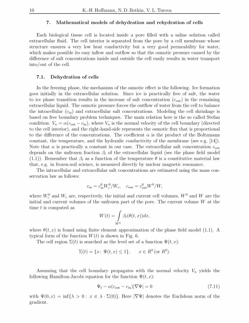
where θ(t, x) is found using finite element approximation of the phase field model (1.1). Atypical form of the function W (t) is shown in Fig. 6.

The cell region Σ(t) is searched as the level set of a function Ψ(t, x):

Σ(t) = x : Ψ(t, x) ≤ 1, x ∈ R3 (or R2).

Assuming that the cell boundary propagates with the normal velocity Vn yields thefollowing Hamilton-Jacobi equation for the function Ψ(t, x):

Ψt − α(cout − cin)|∇Ψ| = 0 (7.11)

with Ψ(0, x) = infλ > 0 : x ∈ λ · Σ(0). Here |∇Ψ| denotes the Euclidean norm of thegradient.

Freezing of living cells 11

W

W 0

t

Figure 6. Evolution of the volume of the unfrozen extracellular liquid versus time.

7.2. Rehydration of cells

In the thawing phase, the osmotic effect results in the cell inflow and hence in cell swelling.We use the following mass conservation law for the salt content:

W 0c c0

in = Ws c0in + Wℓ cin, Wc = Ws + Wℓ, (7.12)

where W 0c is the initial volume of the frozen cell; Wc is the current volume of the cell; Ws

and Wℓ are volumes of the frozen and unfrozen parts of the cell, respectively; c0in and cin

are the salt concentrations in the frozen and unfrozen parts of the cell, respectively. From(7.12), one obtains

cin = c0in

(

1 + (W 0c − Wc)/Wℓ

)

.

We assume that

Wℓ(t) ≈∫

W 0c

βℓ (θ(t, x))dx,

where the function βℓ shows now the volume fraction of unfrozen intracellular fluid. Thesalt concentration cout outside the cell is supposed to be constant.

Admitting that the propagation velocity Vn of the cell boundary is proportional to thedifference of the concentrations cin and cout, one arrives at the equation of the form (7.11).

8. Finite-difference scheme for solving Hamilton-Jacobi equation

Hamilton-Jacobi equation (7.11) is solved numerically using a finite difference schemefor finding viscosity solutions. This section describes a proper scheme. Conventionally, thesymbol |h| denotes the absolute value of h in the case of scalar or the Euclidian norm of hin the case of vector.

Consider a general form of the Hamilton-Jacobi equation (initial value problem) andassume for simplicity that the spatial variable is three dimensional:

Ψt + H(t, x, Ψx) = 0, Ψ(0, x) = σ(x). (8.13)

Here x = (x1, x2, x3) ∈ R3; t ∈ [0,∞); Ψ : [0,∞) × R3 → R; and σ : R3 → R is some givenfunction. Assume that the Hamiltonian H is defined as

H(t, x, p) = maxv∈Q

minu∈P

〈p, f(t, x, u, v)〉,

12 K.-H.Hoffmann, N.D.Botkin, V. L.Turova

where f is the right-hand side of the following conflict controlled system

x = f(t, x, u, v), x ∈ R3, u ∈ P ⊂ Rp, v ∈ Q ⊂ Rq, p, q ≤ 3. (8.14)

The function f is assumed to be uniformly continuous on [0,∞)×R3 ×P ×Q, boundedand Lipschitz-continuous in t, x, the function σ being bounded and Lipschitz-continuous inx.

Let τ, ∆xi, i = 1, 2, 3, are time and space discretization steps. Similar to Section 3,

introduce the notation

Ψn(xi1, x

j2, x

k3) = Ψ(tn, i∆x1

, j∆x2, k∆x3

), tn = nτ

and consider a difference scheme:

Ψn+1(xi1, x

j2, x

k3) = Ψn(xi

1, xj2, x

k3) − τH(tn, xi

1, xj2, x

k3, Ψ

nx1

, Ψnx2

, Ψnx3

)

Ψ0(xi1, x

j2, x

k3) = σ(xi

1, xj2, x

k3).

Here, the symbols Ψnx1

, Ψnx2

, Ψnx3

denote finite difference approximations (left, right, centraland etc.) of the corresponding partial derivatives. Note that the n+1 th function is computedon the base of the n th function, and the Hamiltonian appears with the sign “-” in contrastto Section 3 because the initial value problem is studied.

The scheme can be considered as the successive application of an operator Π to the gridfunctions:

Ψn+1 = Π(Ψn; tn, τ, ∆x1, ∆x2

, ∆x3).

Note that such an operator can be naturally extended to continuum functions. Let usremember the monotonicity and generator properties (comp. Section 3) of the operator Π.The definition of monotonicity is just the same as in Section 3. The generator property isformulated similar to that from Section 3 but with the sign “+” in front of the Hamiltonian,i.e.

∣

∣

∣

∣

Π(φ; t, τ, a1τ, a2τ, a3τ)(x) − φ(x)

τ+ H(t, x, Dφ(x))

∣

∣

∣

∣

≤ C(

1 + ‖Dφ‖ + ‖D2φ‖)

τ

for smooth functions φ (see Section 3).

Theorem 2. (convergence, [19]). Assume that the operator Π(·; t, τ, a1τ, a2τ, a3τ) ismonotone for any t, τ > 0 and satisfies the generator property, then the grid function ob-tained by the procedure:

Ψn+1 = Π(Ψn; t, τ, a1τ, a2τ, a3τ), n = 0, 1, ..., Ψ0 = σ,

converges point-wise to a viscosity solution of Hamilton-Jacobi equation (8.13) as τ → 0,and the convergence rate is

√τ .

We consider an upwind finite difference scheme similar to that given in Section 4 (dis-tinctions arise because of the initial value problem formulation):

Π(Ψn; tn, τ, ∆x1, ∆x2

, ∆x3)(xi

1, xj2, x

k3) = Ψn(xi

1, xj2, x

k3) − τ max

v∈Qminu∈P

3∑

m=1

(pLm · f+

m + pRm · f−

m),

(8.15)

Freezing of living cells 13

where f1, f2, f3 are the right hand sides of system (8.14) computed at (tn, xi1, x

j2, x

k3, u, v);

pR1 , pR

2 , pR3 and pL

1 , pL2 , pL

3 the right and the left divided differences, respectively. The argu-ments tn, xi

1, xj2, x

k3, u, v of f−

m and f+m are omitted for brevity.

Let us prove that the operator Π meets the requirements of Theorem 2. The followinglemmas hold.

Lemma 2. (monotonicity). Let M be the bound of |f |. If a1, a2, a3 ≥ M√

3, then theoperator Π(·; t, τ, aτ, bτ, cτ) given by (8.15) is monotone.

Proof. Suppose Ψ ≤ Φ. Let us show that Π(Ψ; t, τ, a1τ, a2τ, a3τ) ≤ Π(Φ; t, τ, a1τ, a2τ, a3τ).Denote h1 = (a1, 0, 0), h2 = (0, a2, 0), h3 = (0, 0, a3). We have

Π(Ψ; t, τ, a1τ, a2τ, a3τ)(x) − Π(Φ; t, τ, a1τ, a2τ, a3τ)(x) = Ψ(x) − Φ(x)

− τ maxv∈Q

minu∈P

3∑

m=1

(Ψ(x) − Ψ(x − hmτ)

amτf+

m +Ψ(x + hmτ) − Ψ(x)

amτf−

m

)

+ τ maxv∈Q

minu∈P

3∑

m=1

(Φ(x) − Φ(x − hmτ)

amτf+

m +Φ(x + hmτ) − Φ(x)

amτf−

m

)

.

By rearranging terms and using the obvious relations f+m −f−

m = |fm| and maxv

minu

g1(u, v)−max

vmin

ug2(u, v) ≤ max

vmax

u

[

g1(u, v) − g2(u, v)]

, one obtains

Π(Ψ; t, τ, a1τ, a2τ, a3τ)(x) − Π(Φ; t, τ, a1, a2, a3)(x) ≤ Ψ(x) − Φ(x)

+ τ maxv∈Q

maxu∈P

3∑

m=1

[(Ψ(x − hmτ) − Φ(x − hmτ)

amτ− Ψ(x) − Φ(x)

amτ

)

f+m

+(Ψ(x + hmτ) − Φ(x + hmτ)

amτ− Ψ(x) − Φ(x)

amτ

)

(−f−m)

]

≤ Ψ(x) − Φ(x) − τ

3∑

m=1

|fm|amτ

(

Ψ(x) − Φ(x))

=(

1 −3

∑

m=1

|fm|am

)

(

Ψ(x) − Φ(x))

.

With3

∑

m=1

|fm| ≤√

3M one comes to 1 −3

∑

m=1

|fm|am

> 0, which finally implies the required

inequality.

Lemma 3. (generator property). The generator property holds for the operator Π.

Proof. Let φ ∈ C2b (R

3). Denote d1 = (∆x1, 0, 0), d2 = (0, ∆x2

, 0), d3 = (0, 0, ∆x3). We

have

Π(φ; t, τ, ∆x1, ∆x2

, ∆x3)(x) = φ(x) − τ max

v∈Qminu∈P

3∑

m=1

(φ(x) − φ(x − dm)

∆xm

f+m +

φ(x + dm) − φ(x)

∆xm

f−m

)

.

14 K.-H.Hoffmann, N.D.Botkin, V. L.Turova

Estimate

∣

∣

∣

Π(φ; t, τ, ∆x1, ∆x2

, ∆x3)(x) − φ(x)

τ+ max

v∈Qminu∈P

〈Dφ(x), f〉∣

∣

∣

=∣

∣

∣− max

v∈Qminu∈P

3∑

m=1

(φ(x) − φ(x − dm)

∆xm

f+m +

φ(x + dm) − φ(x)

∆xm

f−m

)

+ maxv∈Q

minu∈P

3∑

m=1

∂φ

∂xm

(f+m + f−

m)∣

∣

∣

≤ maxu∈P

maxv∈Q

3∑

m=1

∣

∣

∣

( ∂φ

∂xm

− φ(x) − φ(x − dm)

∆xm

)

f+m +

( ∂φ

∂xm

− φ(x + dm) − φ(x)

∆xm

)

f−m

∣

∣

∣

≤ M ‖D2φ‖3

∑

m=1

∆xm.

Here M is the bound of |f |. Choosing ∆xm= amτ and letting C =

3∑

m=1

am yields

∣

∣

∣

Π(φ; t, τ, ∆x1, ∆x2

, ∆x3)(x) − φ(x)

τ+ H(t, x, Dφ(x)

∣

∣

∣≤ M C ‖D2φ ‖ τ.

9. Three dimensional simulation of cell shrinkage

The finite difference scheme based on the operator Π is implemented as a parallelizedprogram on a Linux cluster. We compute the evolution of the cell boundary during freezing.The function f in our case is

f(t, u, v) = α(

cout(t) − cin(t))+

u + α(

cout(t) − cin(t))−

v, u, v ∈ R3, |u| ≤ 1, |v| ≤ 1.

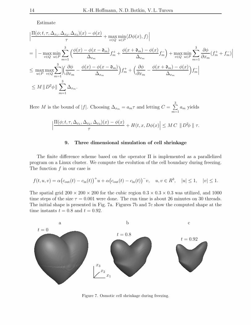
The spatial grid 200 × 200 × 200 for the cubic region 0.3 × 0.3 × 0.3 was utilized, and 1000time steps of the size τ = 0.001 were done. The run time is about 26 minutes on 30 threads.The initial shape is presented in Fig. 7a. Figures 7b and 7c show the computed shape at thetime instants t = 0.8 and t = 0.92.

a b c

t = 0t = 0.8

t = 0.92

x3

x1

x2

Figure 7. Osmotic cell shrinkage during freezing.

Freezing of living cells 15

10. Accounting for the membrane tension using reachable set approach

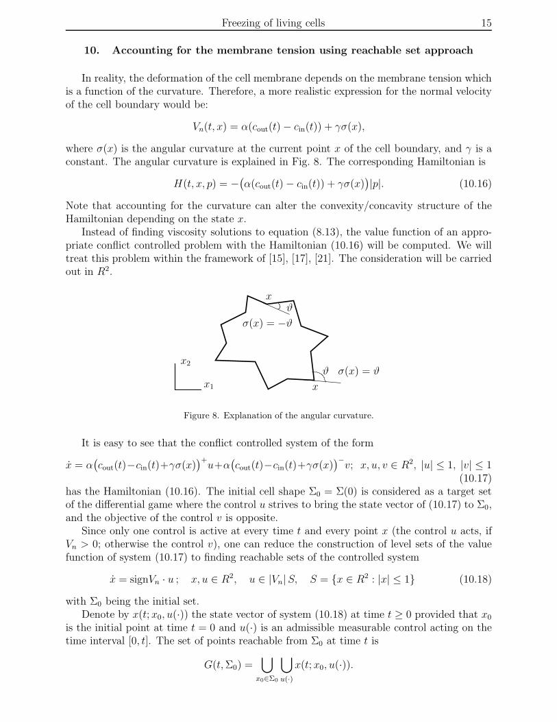
In reality, the deformation of the cell membrane depends on the membrane tension whichis a function of the curvature. Therefore, a more realistic expression for the normal velocityof the cell boundary would be:

Vn(t, x) = α(cout(t) − cin(t)) + γσ(x),

where σ(x) is the angular curvature at the current point x of the cell boundary, and γ is aconstant. The angular curvature is explained in Fig. 8. The corresponding Hamiltonian is

H(t, x, p) = −(

α(cout(t) − cin(t)) + γσ(x))

|p|. (10.16)

Note that accounting for the curvature can alter the convexity/concavity structure of theHamiltonian depending on the state x.

Instead of finding viscosity solutions to equation (8.13), the value function of an appro-priate conflict controlled problem with the Hamiltonian (10.16) will be computed. We willtreat this problem within the framework of [15], [17], [21]. The consideration will be carriedout in R2.

xϑ

σ(x) = −ϑ

x

ϑ σ(x) = ϑx2

x1

Figure 8. Explanation of the angular curvature.

It is easy to see that the conflict controlled system of the form

x = α(

cout(t)−cin(t)+γσ(x))+

u+α(

cout(t)−cin(t)+γσ(x))−

v; x, u, v ∈ R2, |u| ≤ 1, |v| ≤ 1(10.17)

has the Hamiltonian (10.16). The initial cell shape Σ0 = Σ(0) is considered as a target setof the differential game where the control u strives to bring the state vector of (10.17) to Σ0,and the objective of the control v is opposite.

Since only one control is active at every time t and every point x (the control u acts, ifVn > 0; otherwise the control v), one can reduce the construction of level sets of the valuefunction of system (10.17) to finding reachable sets of the controlled system

x = signVn · u ; x, u ∈ R2, u ∈ |Vn|S, S = x ∈ R2 : |x| ≤ 1 (10.18)

with Σ0 being the initial set.Denote by x(t; x0, u(·)) the state vector of system (10.18) at time t ≥ 0 provided that x0

is the initial point at time t = 0 and u(·) is an admissible measurable control acting on thetime interval [0, t]. The set of points reachable from Σ0 at time t is

G(t, Σ0) =⋃

x0∈Σ0

⋃

u(·)

x(t; x0, u(·)).

16 K.-H.Hoffmann, N.D.Botkin, V. L.Turova

The algorithm for the numerical construction of the sequence Gi = G(i∆t,Gi−1), i =1, 2, ..., G0 = Σ0, is similar to that one described in [18]. The difference is that the treatmentof the cases of local concavity and local convexity alters depending on the sign of Vn.

Simulation results showing the time evolution of the cell shape during freezing are pre-sented in Fig. 9. The sequence of reachable sets is computed on the time interval [0, 0.645]with the time step ∆t = 0.001, every fourth set is drawn. The restriction on the controlis u ∈ |Vn|P · S, where P = pij is the 2 × 2- diagonal matrix introducing anisotropy(p11 = 3, p22 = 1). For the left picture, γ = 0 , i.e. the curvature independent case is

Σ0

x2

x1

Figure 9. Time evolution of the cell during freezing. To the left: without accounting for the curvature. Tothe right: with accounting for the curvature.

considered. For the right picture, γ = 0.06. Note that the low propagation velocity at thebeginning of the process results in the accumulation of lines (dark regions) near the initialcell boundary.

In Figure 10, an example of the simulation of cell rehydration during thawing is presented.The computation is done on the time interval [0, 9.7] with the time step ∆t = 0.002. Every100th reachable set is drawn. At the finish of the process the stabilization of sets is observeddue to the achieved equilibrium of salt concentrations inside and outside the cell.

Σ0

x2

x1

Figure 10. Time evolution of the cell during thawing with accounting for the curvature.

Freezing of living cells 17

11. Conclusion

Problems considered in the paper show that spatially distributed models can be reducedto optimal control problems for ordinary differential equations with control parameters anddisturbances using appropriate averaging techniques. Because of tabular form of nonlineardependencies appearing in the right-hand sides of such equations, the application of Pon-tryagin’s maximum principle is complicated, whereas appropriate grid methods or reachableset techniques do work here. The usage of stable algorithms allows us to obtain convincingresults. Optimal cooling protocols designed can be implemented in real cooling devices suchas e.g. IceCube developed by SY-LAB, Gerate GmbH (Austria).

REFERENCES

1. Batycky R.P., Hammerstedt R., Edwards D.A. Osmotically driven intracellular transport phe-nomena // Phil. Trans. R. Soc. Lond. A. 1997. Vol. 355. P. 2459–2488.

2. Botkin N.D. Approximation schemes for finding the value functions for differential games with non-terminal payoff functional// Analysis 1994. Vol. 14, no. 2. P. 203–220.

3. Botkin N.D., Hoffmann K-H., Turova V.L. Stable Solutions of Hamilton-Jacobi Equations. Ap-plication to Control of Freezing Processes. German Research Society (DFG), Priority Program 1253:Optimization with Partial Differential Equations. Preprint-Nr. SPP1253-080 (2009).http://www.am.uni-erlangen.de/home/spp1253/wiki/images/7/7d/Preprint-SPP1253-080.pdf

4. Caginalp G. An analysis of a phase field model of a free boundary // Arch. Rat. Mech. Anal. 1986.Vol. 92. P. 205–245.

5. Chen S.C., Mrksich M., Huang S., Whitesides G.M., Ingber D.E. Geometric control of cell lifeand death //Science. 1997. Vol. 276. P. 1425–1428.

6. Crandall M.G., Lions P.L. Viscosity solutions of Hamilton-Jacobi equations //Trans. Amer. Math.Soc. 1983. Vol. 277. P. 1–47.

7. Crandall M.G., Lions P.L. Two approximations of solutions of Hamilton-Jacobi equations //Math.Comp. 1984. Vol. 43. P. 1–19.

8. Fremond M. Non-Smooth Thermomechanics. Berlin: Springer-Verlag, 2002. 490 p.9. Hoffmann K.-H., Jiang Lishang. Optimal control of a phase field model for solidification //Numer.

Funct. Anal. Optimiz. 1992. Vol. 13, no. 1,2. P. 11–27.10. Hoffmann K.-H., Botkin N.D. Optimal control in cryopreservation of cells and tissues//in: Pro-

ceedings of Int. Conference on Nonlinear Phenomena with Energy Dissipation. Mathematical Analysis,Modeling and Simulation, Colli P. (ed.) et al, Chiba, Japan, November 26–30, 2007. Gakuto InternationalSeries Mathematical Sciences and Applications 29, 2008. P. 177–200.

11. Hoffmann K.-H., Botkin N.D. Optimal Control in Cryopreservation of Cells and Tissues, Preprint-Nr.: SPP1253-17-03. 2008.

12. Isaacs R. Differential Games. New York: John Wiley, 1965. 408 p.13. Malafeyev O.A., Troeva M.S. A weak solution of Hamilton-Jacobi equation for a differential two-

person zero-sum game, in: Preprints of the Eight Int. Symp. on Differential Games and Applications,Maastricht, Netherland, July 5-7, 1998, P. 366–369.

14. Mao L., Udaykumar H.S., Karlsson J.O.M. Simulation of micro scale interaction betweenice andbiological cells // Int. J. of Heat and Mass Transfer. 2003. Vol. 46. P. 5123–5136.

15. Krasovskii N.N, Subbotin A.I. Positional Differential Games. Moscow: Nauka, 1974. p. (in Russian).16. Krasovskii N.N. Control of a Dynamic System. Moscow: Nauka, 1985. 520 p. (in Russian).17. Krasovskii N.N., Subbotin A.I. Game-Theoretical Control Problems. New York: Springer, 1988.

518 p.18. Patsko V.S., Turova V.L. From Dubins’ car to Reeds and Shepp’s mobile robot // Comput. Visual.

Sci. 2009. Vol. 13, no. 7. P. 345–364.19. Souganidis P.E. Approximation schemes for viscosity solutions of Hamilton-Jacobi equations //J.

Differ. Equ. 1985 Vol. 59. P. 1–43.20. Subbotin A.I., Chentsov A.G. Optimization of Guaranteed Result in Control Problems. Moscow:

Nauka, 1981. 287 p. (in Russian).21. Subbotin A.I. Generalized Solutions of First Order PDEs. Boston: Birkhauser, 1995. 312 p.