Trends in the Size Distribution of Wealth in the ...piketty.pse.ens.fr/files/Gallman1969.pdf · the size distribution of wealth in the U. S. in 1860, following the ... of the Wealthy

This PDF is a selection from an out-of-print volume from the National Bureau of Economic Research

Volume Title: Six Papers on the Size Distribution of Wealth and Income

Volume Author/Editor: Lee Soltow, ed.

Volume Publisher: NBER

Volume ISBN: 0-870-14488-X

Volume URL: http://www.nber.org/books/solt69-1

Publication Date: 1969

Chapter Title: Trends in the Size Distribution of Wealth in the Nineteenth Century: Some Speculations

Chapter Author: Robert E. Gallman

Chapter URL: http://www.nber.org/chapters/c4339

Chapter pages in book: (p. 1 - 30)

Trends in the Size Distribution of Wealth

in the Nineteenth Century: Some Speculations

ROBERT E. GALLMANUNIVERSITY OF NORTH CAROLINA

AT PRESENT there are afoot two major studies (by Alice Jones ofWashington University, and Lee Soltow of Ohio University) that, whencompleted, will tell us a good deal about the structure of wealthholdings toward the end of the eighteenth century and just before theCivil War. Until these studies are available, judgements concerningtrends in the size distribution of wealth in the nineteenth century mustrest on evidence by no means as full as one would wish. Nevertheless,some data are available and they suggest findings sufficiently clear andinteresting to warrant a discussion at this time.

I propose to do the following: (1) compute from fragmentary censusdata a size distribution of wealth for the United States in 1860;(2) estimate the responsibility of the, slave system for the shape ofthe 1860 distribution; (3) show the effect of trends in the distributionof population among three locations—large cities, the plantation south,other rural 1 areas—on the size distribution of wealth, on the assump-tion that all other relevant factors remain constant; (4) incorporateinto the preceding analysis an estimate of the direction and weight ofthe effect of changes in average urban and rural wealth holdings onthe size distribution of wealth; (5) estimate directly, using somewhatdifferent data, the trend of the share of wealth held by those at thevery tip of the wealth pyramid.

NOTE: I would like to thank Karen Hensely, Anne Cobb, Dale Swan, andDonald Schaefer, who helped me with the wealth samples drawn from themanuscript census; Taylor Cousins, who assembled the evidence from the pam-phlets of Moses Beach; and my wife, Jane, who helped me to test the manuscriptcensus samples. Both ray wife and William N. Parker kindly listened to my plansand offered criticism.

1 The term "rural" is used in this chapter to designate areas outside largecities (i.e., those with at least 40,000 in population).

2 Distribution Trends in Nineteenth Century

The results of these exercises will suggest that the share of wealthheld by the rich probably drifted upward during the nineteenth century,the support for this statement being stronger for the latter half of thecentury than for the first half.

I. Wealth Distribution in the U. S., 1860The appendix contains wealth distributions for three cities and threerural areas, computed from the manuscript census records of 1860. Ifthese distributions can be regarded as representative of larger popula-tions, the total exhausting the universe, they can be used to computethe size distribution of wealth in the U. S. in 1860, following theprocedure proposed in another context by Professor Kuznets.2 Meanwealth per family is computed for each subuniverse, and relativeweights are established on this basis. Each sample distribution (ex-pressed in terms of the per cent of wealth held by each percentile ofthe family population) is then multiplied by the relevant weight. Thedistributions can then be combined into an aggregate distribution. Thenumber of times each sample enters into the aggregate distributiondepends upon the fraction of families in the universe represented bythe sample. It will be convenient subsequently to speak of the firstoperation as the application of a "wealth weight"; the second, theapplication of a "population weight." A simple example will clarifythe procedure.

Assume that we have two samples, each adequately representing oneof the two components of the universe under study. Suppose that wewant to find out the shares of wealth held by the four quartiles of theuniverse. The sample distributions are as follows:

A B

First quartile 90% 75%Second quartile 8 15.Third quartile 2 8Fourth quartile 0 2

Suppose that wealth held per family in the component represented byB is twice the value of wealth held per family in the component

2 Simon Kuznets, "Economic Growth and Income Inequality," The AmericanEconomic Review, March 1955.

Distribution Trends in Nineteenth Century 3

represented by A. Suppose, further, that B represents three times asmany families as A. Then we multiply the B distribution by two andenter it into the calculations three times, to produce wealth holdingsof the quartiles of the universe:

First quartile 150+150+150+90=540Second quartile 30+ 30+ 30+16= 106Third quartile 16+ 16+ 8+ 4 = 44Fourth quartile 4+ 4+ 2+ 0= 10

700

Dividing through by seven yields the following percentile distributionfor the universe:

First quartile 77%Second quartile 15Third quartile 6Fourth quartile 1

100 (99, due to rounding)

Now the evidence assembled in the appendix suggests that in 1860the distribution of wealth was much more unequal in large cities thanin rural areas, the contrast being especially striking when one considersthe shares of wealth held by the richest 1 per cent of families. Addi-tionally, while wealth per family varied somewhat from city to cityand state to state, the only truly striking differences appear when onecompares average wealth per family in the plantation South with averagewealth per family elsewhere. In the sugar, rice and cotton territoriesof the South wealth per family ran about $12,000, whereas in the restof the country it averaged about $3,000. The evidence relating to thedistribution of wealth and average holdings per family suggest, then,that for purposes of assembling a size distribution for the country asa whole one can work effectively with samples drawn from three sub-universes: cities, the plantation South, and other rural areas. Thequestion then arises as to how representative the samples provided inthe appendix are in fact.

So far as the plantation South is concerned, we lack only a samplefrom the rice economy. However, the weight such a sample wouldhave in determining the aggregate distribution would, necessarily, be


very small. Furthermore, the distribution within the rice economy isnot likely to differ markedly from the distribution within the sugareconomy, an4 we do have evidence relating to the latter. The Louisianasample can be treated as roughly representative of both the sugar andrice economies.

We have samples relating to the third, fifth and seventh largest citiesin the U. S. in 1860. The three cities are quite different, in terms ofgeography, hinterlands, and industrial mix. One is an old East Coastport; the second, a gulf port, outlet for western goods and the productsof the plantation South; the third, a western river city, located withinan important trading nexus but also heavily committed to manufactur-ing.3 The three are quite different, yet they exhibit essentially the samewealth distribution, suggesting that the composite distribution for thethree may be broadly representative of large cities.4 How far down thescale of size the distribution remains representative, we have no wayof knowing. We arbitrarily assume that the distribution for the threesampled cities adequately represents the distribution in the largesttwenty cities, the smallest of which had a population of 43,000 in

The very rich in this city tended to be manufacturers, whereas in Baltimoreand New Orleans they were more often merchants.

4 perhaps not for very large cities. The richest 1,062 families in New YorkCity in 1855 held property equal in value to about 62 per cent of the wealthreturned at the Census of 1860 by all New York citizens, according to MosesBeach. (The Wealthy Citizens of New York, 12th Edition, New York, 1855.)This group accounted for between .6 and .7 per cent of the families in New York.The combined distributions of Baltimore, St. Louis, and New Orleans (AppendixTable 1, "Three Cities, Adjusted") attributes 45 per cent of the wealth held byfamilies in large cities to the richest 1 per cent of families. Beach's estimate ofthe wealth-holdings of the richest 1,062 families in New York may be excessiveand, additionally, the census return of property owned by New Yorkers in 1860may be somewhat too low. Nonetheless, there appears to be good reason tobelieve that wealth concentration in New York was greater than in other cities.Therefore, we developed a separate distribution intended to reflect circumstancesin New York. See the notes to Table 1.

According to "A Member of The Philadelphia Bar" (Wealth and Biographyof the Wealthy Citizens of Philadelphia, by a Member of the Philadelphia Bar,1845) the richest 711 families in Philadelphia held property valued at about$75 million in 1845. The 1860 Census (Population, p. XVIII) returns 101,361families in Philadelphia County, owning about $394 millions of property. Thesetwo scraps of information suggest that it is unlikely that the richest 1 per centof families in Philadelphia owned substantially more or less than 45 per centof wealth owned by Philadelphians in 1860. We therefore assume that thecombined distribution of the three sample cities adequately represents circum-stances in Philadelphia.


Our ultimate results are not unduly sensitive to the preciselocation of the cutoff point. Had we confined the definition of "largecities" to the largest fifteen, or expanded it to include the largestthirty-five, our ultimate results would not have been markedly different.

We are left, then, with the "all other rural areas" subuniverse. Theonly sample we have relating to the subuniverse is the sample ofMaryland, outside Baltimore. To treat the Maryland sample as rep-resentative of so large, and perhaps heterogeneous, a territory mayappear outrageous; however, several good reasons can be advanced fordoing so. First, the sample may very well be roughly representative ofan important part of the "all other" subuniverse, the upper South andMiddle Atlantic States.6 Second, if the Maryland sample is unrepre-sentative, we can be quite sure that it exhibits a distribution somewhatmore unequal than the distribution appropriate to the "all other" sub-universe.7 Therefore, we can specify the direction of bias in thecomputed distribution for the United States. Third, the principal objectof constructing the U. S. distribution for 1860 is to provide the meansof investigating the effects of structural changes of various kinds onthe wealth distribution. For that purpose a precisely accurate distribu-tion is not required, since we are less concerned with levels of concen-tration than with changes in concentration. Finally, with respect to thelevel of concentration, the proof of any pudding is in the eating. Theone check we have on the estimates generated in this paper tends toconfirm our results (see below).

Accepting the sample distributions as sufficiently representative, wecompute the distribution identified as 1860 A in Table 1.

Most of the census data on wealth and family population are reported bycounty, rather than by city. The wealth and population weights we used, therefore,relate to the counties in which the largest twenty cities are located. Consequentlyour population weights give to the "three cities" distribution an importance some-what greater than the text suggests.

6 Additionally, the agricultural characteristics of the sample and the subuniverseare presumably of special importance. Leaving out the two relatively new statesof California and Oregon, the average size of farm varied from state to statein the non-South within the fairly narrow range of 99—211 acres. The averagein Maryland falls within this range, at 199 acres. Whereas in the South (Alabama,Arkansas, Florida, Georgia, Louisiana, Mississippi, North Carolina, South Caro-lina, Tennessee, Texas, Virginia) the range was from 245—591. (Census of 1860,Agriculture, p. 222.)

See, for example, the distribution of farms by size of farm, Census of 1860,Agriculture, p. 221.


TABLE 1

ESTIMATES OF THE SIZE DISTRIBUTION OF WEALTH IN THE UNITEDSTATES IN 1860 AND PROJECTIONS TO 1810 AND 1900

(per cent)

Families

Shares in Personally Mel d Wealth a

1810 1860 A 1860 B 1900 C 1900 D

First (richest)percentile 21 24 24 26 31

Second percentile 11 11 11 11 11

Third percentile 8 8 7 7 7

Fourth percentile 6 6 6 6 6Fifth percentile 5 5 5 5 5

Sixth percentile 4 4 5 4 4Seventh percentile 4 4 4 4 3

Eighth percentile 3 3 4 4 3

Ninth percentile 3 3 3 3 - 3

Tenth percentile 3 3 3 2 2

First decile 69 71 72 73 74Second decile 17 16

Third decile 7 7

Fourth decile 3 2Fifth decile I I

First half 100 100Second half 0 0

SOURCES: 1860 A — Five sample distributions were combined in the manner describedin the text. Four of the distributions were taken from Appendix Table A-i ("Three Cities,Adjusted"; Maryland, cx Baltimore; Louisiana, ex New Orleans, and "Cotton Coun-ties"). The fifth distribution (taken to represent New York City) is similar to the "threecities, adjusted" distribution, except that the richest I per cent is assumed to own 55 percent of the wealth. The basis for the "New York" distribution is described in text foot-note 4.

The two distributions, Louisiana (ex New Orleans) and "cotton counties," were eachgiven a wealth weight of 4. All other distributions received a wealth weight of 1. (Seetext.)

The population weights (see text), which are based on the number of free familiesrepresented by each distribution, are as follows:

Louisiana (cx New Orleans) 2Cotton Counties 6New York City 3

"Three Cities, Adjusted" 12Other Rural Areas 77


TABLE I SOURCES (continued)Southern rural areas receive slightly too heavy a weight, since several cotton countiesare represented in both the "cotton counties" distribution and the Louisiana (ex NewOrleans) distribution (the latter taken to be representative of rural Louisiana and SouthCarolina).

1860 B — The distribution differs from 1860 A only in that slaves are regarded as po-tential property owners, not as property. The text describes the procedure by which the1860 A distribution was adjusted to produce the 1860 B distribution. In order to makethe adjustments we had to estimate (for Louisiana, ex New Orleans, South Carolina, andthe Cotton County sample):

1 — the value of slaves2— the number of slave families3—the size distribution of nonslave wealth.

We estimated the relevant slave values from the number of slaves returned at the cen-sus in Louisiana (ex New Orleans) and South Carolina and the number covered in theCotton County sample, together with an estimated value per slave of $900.

We computed the number of slave families in Louisiana (ex New Orleans) plus SouthCarolina and in the Cotton County sample by multiplying each slave population by theratio of free families to free population in the relevant area.

Average wealth per family (free and slave) came to a value, in each case, close to thevalue of average wealth per family in the non-South. Consequently, each distributionwas given a wealth weight of I in the calculation of the national distribution.

The population weights were necessarily revised:Louisiana (ex New Orleans) 5

Cotton Counties 12New York City 3

"Three Cities, Adjusted" 10Other Rural Areas 70

We assumed that the ratio of slave families to free families derived for Louisiana (exNew Orleans) and South Carolina was also relevant to the Louisiana (ex New Orleans)sample and in this way estimated the number of slave families covered by the sample.

We assumed that slave families owned no property and therefore could be introducedat the bottom of the wealth distributions.

We assumed that total nonslave property was distributed among wealth-holdingfamilies exactly as was the value of real property. Since both samples distinguish realproperty', we were then able to compute wealth distributions for nonslave wealth. Ourresults are as follows:

Louisiana(ex New CottonOrleans) Counties

First (richest)percentile 50% 30%

Second percentile 15 11

Third percentile 9 7

Fourth percentile 6 5

Fifth percentile 4 5

Sixth percentile 4 4Seventh percentile 3 4Eighth percentile 2 4Ninth percentile 2 3

Tenth percentile I 3

First decile 96 79

8 Distribution Trends in Nineteenth Centu,y

TABLE 1 SOURCES (concluded)1810—The 1860 A distributions were combined, but by means of population weights

presumably relevant to 1810. We assumed that in 1810 the "Three Cities, Adjusted" dis-tribution was relevant to all large cities, including New York. We projected the 1860weights backward on the following population series: Cities over 50,000; Louisiana andSouth Carolina; Georgia, Alabama, Mississippi; All others. (Historical Statistics, TablesA 123—180 and 195—207.)

Ideally, the extrapolating series would refer to only free population. However, the im-provement in results over those achieved by total population series (used here) wouldbe negligible.

The weights generated are as follows:Louisiana (ex New Orleans) 4Cotton Counties 3

"Three Cities, Adjusted" 3

Other Rural Areas 901900 C—Computed in exactly the same way as the 1810 distribution, except that the

1860 B distributions were used and the New York City distribution was taken to repre-sent all cities of 1,000,000 population or more. The population weights assigned are:

Louisiana (ex New Orleans) 4Cotton Counties 9New York City 9"Three Cities, Adjusted" 13Other Rural Areas 65

/900 D—Computed in exactly the same way as the 1900 C distribution, except thatthe New York City and "Three Cities, Adjusted" distributions were each assigned awealth weight of 2.

a Details may not add to totals, due to rounding.

1!. Effect of the Slave System on the DistributionThe 1860 A distribution is affected by the existence of the slavesystem in the South. We can judge the significance of the slave systemin this context by recomputing the distribution and treating slaves notas property, but as potential property owners. The calculation hasinterest since it represents a convenient approach to the assessment ofthe effect of abolition on the 4istribution of wealth. Additionally, weneed the distribution in order to draw appropriate comparisons withexperience at the end of the century.8

8A sample drawn from the 1870 census would presumably show the fulleffects of abolition and the Civil War. We have not yet drawn an 1870 samplefor the South and there is some question as to whether the project would befruitful. The population census was notoriously defective in the South in 1870.One would anticipate that questions relating to wealth would be especiallyresisted, not only in the South, but also in the North, in view of tax developmentsduring the War. However, it is by no means certain that the wealth returns areunworthy of investigation. Preliminary work with the St. Louis, Baltimore and


If slaves are treated as property holders, rather than as property,each of the three steps in the calculation of the national wealthdistribution is affected.

1. The value of slaves must be deducted from the census reports ofthe value of property owned in the plantation South, and the numberof families augmented by the number of slave families.9 Both operationsreduce the value of wealth per family in the plantation South and,therefore, the wealth weights assigned to the Southern distributions.

2. However, if slaves are treated as potential property holders, theneach of the two Southern distributions represents a larger populationof families and therefore must receive a larger population weight inthe calculation of the national distribution.

3. Finally, the Southern distributions are altered, both because alarge number of propertyless families (slaves) are introduced into theuniverse of families and because the definition of wealth is narrowed.

The detailed procedures followed to carry out the adjustments tothe 1860 A distribution described above are contained in the notesto Table 1. It is sufficient to say here that the effect of the changein the Southern wealth weight is opposite in direction, and almostexactly compensates for, the effects of the changes in the Southerndistributions and population weights. Consequently, the adjusted dis-tribution, 1860 B, is virtually identical to the original distribution,1860 A. The size distribution of wealth in the United States in 1860is almost entirely independent of the convention adopted for the handlingof slaves. Virtually the same national distribution eventuates when slavesare treated as potential property owners as when they are treated asproperty.

Ill. Effect of Population Trends on the DistributionThe 1860 size distributions for the U. S. were computed by applyingpopulation and wealth weights to sample distributions. The analysis oftrends in the size distribution can be organized in the same way. That

New Orleans schedules suggests that at least the first two may warrant furtherexamination. We have drawn small samples from each and they yield distributionssimilar to those obtained for these cities in 1860.

were held in two of the three sampled cities, but their number andvalue were not appreciable and therefore we confine the adjustment to the samplesrelating to the plantation South.


is, we can conceive of three factors affecting the size distribution acrosstime: (1) trends in population weights, (2) trends in wealth weights,(3) trends in the distributions within the sampled universes. Evidencewith respect to the last two factors is difficult to come by. This paperoffers none bearing on the last 10 and very little relating to the second,but it is a simple enough matter to measure the effects of changingpopulation weights on the size distribution. Adequate population seriesby which the weights of 1860 may be extrapolated to other years arereadily available. Table 1 contains estimates for 1810 and 1900(1900 C) computed from the 1860 sample distributions and wealthweights, together with population weights relevant to 1810 and 1900.We have projected the 1860 A distribution backward to 1810 and the1860 B distribution forward to 1900. Details are contained in thenotes to the table.

The estimates indicate that changing population weights operated inthe direction of increasing the share of wealth held by the richest 1per cent of families. But the shares of the other members of the richestdecile are virtually unaffected. The impact on the share of wealth heldby the richest dedile is very slight, indeed. The share rises over theninety year period from 1810 to 1900 by only 4 percentage points,against an original holding of 69 per cent.

How far the wealth weights shifted over time we do not know. How-ever, there is some basis for the presumption that wealth per family inthe cities rose relative to wealth per family in the countryside, at leastafter 1860. For example, between 1860 and 1900 the population ofcities of 50,000 and over increased roughly five-and-a-halffold, whilethe value of national assets, other than agricultural assets, increasedalmost ninefold, intangible assets, by perhaps thirteenfold, and tangibleassets of industry, commerce and public utilities, by roughly seven-and-a-halffold. On the other hand, the population outside these cities morethan doubled, while the value of agricultural assets increased by onlytwo-and-a-halffold.11 Clearly, this evidence does not bear directly onthe value of property owned by city dwellers and those outside large

10 But see footnote 8.11 The wealth data (current prices) are from Robert E. Gailman, "The Social

Distribution of Wealth in the United States of America," paper delivered to theInternational Economic History Congress, Munich, 1965; the population data,from Historical Statistics, Series A-195 through A-209.


cities. However, it may represent a reasonable guide as to the directionof change of relative wealth-holdings of these groups. If it does, thenwealth per family in large cities increased relative to wealth per familyoutside these cities over the period 1860 to 1900. How markedly thechange took place, we cannot say. However, it seems reasonable tosuppose that the urban wealth weight in 1900 could not have been asmuch as double the rural weight. We can, therefore, estimate the maxi-mum effect of changing relative wealth weights between 1860 and 1900by recomputing distribution 1900 C, giving the two urban distributionswealth weights of 2 and the rural distributions, wealth weights of 1.Distribution 1900 D, in Table 1, was computed in this way. The impactof the adjustments is confined almost entirely to the share of the richest1 per cent of families, where it is substantial. The share of wealth heldby the richest decile is almost identical in the 1900 C and D distribu-tions.

The exercises with changing population and wealth weights suggestthat there were forces at work in the American economy during thenineteenth century that tended to produce greater inequality in the dis-tribution of wealth over time. The impact of these forces is seen mostclearly when one focuses on the share of wealth held by the richest 1per cent of families. We therefore turn to another body of evidence thatbears directly on the wealth holdings of the very rich, in the hope offinding a means of appraising these results. But before moving on to thisevidence, it is worth remarking that in at least one important particular

wealth distributions projected to 1900 are roughly confirmed by theestimate of another worker. According to G. K. Holmes,

the richest 9 per cent of families in 1890 owned 71 per cent of per-1ield wealth in the United States, a rather remarkable confinna-

tion of the achieved in this paper.12

IV. Other Wealth DistributionsDuring the teenth century various lists of rich families were drawnup, sometimes including estimates of the fortunes of these families anda few biographical notes concerning their members. Holmes used such alist as the basis of his estimate that the millionaire families in the United

12 See C. L. Merwin, Jr., "American Studies of the Distribution of Wealthand Income by Size," Studies in Income and Wealth, Volume 3, New York,NBER, 1939, p. 6.


States owned $12 billion of property in 1890.13 According to Watkins,the list Holmes used was reasonably accurate, but perhaps somewhattoo long.14 We use the Holmes figure, then, to serve as the upper boundof a set of bench-mark estimates for 1890.

If Holmes, in fact, had too many millionaires on his list, we can ad-just his estimate of the value of property held by the richest families inthe country by reducing either the number of very rich families heassumed or his estimate of average wealth per family. We choose tomake two alternative estimates, one based on Holmes' list of 4,000families and an assumed average holding of $2 million; the second,based on Holmes' estimate of the average value of property held bymillionaire families ($3 million) and an estimate of 2,000 millionairefamilies. The bench-mark estimates for 1890 then become: the richest4,000 families owned between $8 and $12 the richest 2,000families $6 billion.

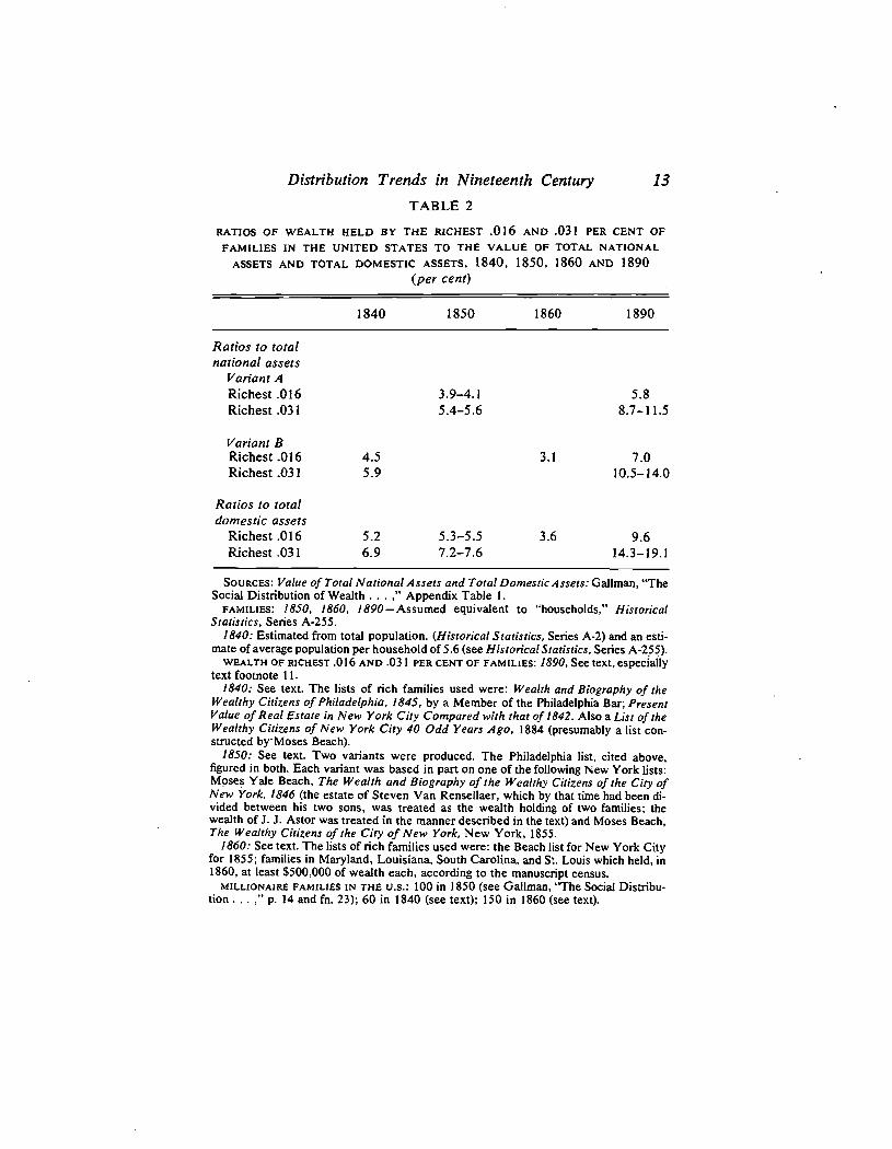
In 1890 there were just under 12.7 million households in the UnitedStates. Consequently, the bench-mark estimates relate to the holdingsof the richest .016 and .031 per cent of American families. The wealthholdings of the richest .031 per cent represent between 9 and 14 percent of total national assets in 1890 and between 14 and 19 per cent ofdomestic tangible assets, while the holdings of the richest .016 per centrepresent between 6 and 7 per cent of total national assets and roughly10 per cent of domestic tangible assets (see Table 2).

Now we want to know whether this degree of concentration character-ized earlier periods of nineteenth century history. Limits on the evidencewe were able to assemble require us to restrict our attention to the years1840, 1850 and 1860.

We have estimates at decade intervals from 1840 onward of the valueof national assets and the value of domestic tangible assets and whilethese figures are, conceptually, imperfect denominators for ratios ofwealth concentration, they appear to be the best available. In any case,we can specify with some certainty the direction of bias over time pro-duced by their use. Without much doubt, they tend to minimize themeasures of concentration for the later years, relative to the earlier

13 Ibid.14 G. P. Watkins, "The Growth of Large Fortunes," Publications of The

can Economic Association, 3rd Series, VIII, 1907, pp. 141, 142.


TABLE 2

RATIOS OF WEALTH HELD BY THE RICHEST .016 AND .031 PER CENT OFFAMILIES IN THE UNITED STATES TO THE VALUE OF TOTAL NATIONAL

ASSETS AND TOTAL DOMESTIC ASSETS, 1840, 1850, 1860 AND 1890(per cent)

1840 1850 1860 1890

Ratios to total

national assets

Variant A

Richest .016Richest .031

3.9—4.15.4—5.6

5.88.7—11.5

Variant BRichest .016Richest .031

4.5

5.9

3.1 7.010.5—14.0

Ratios to totaldomestic assets

Richest .016Richest .031

5.26.9

5.3—5.57.2—7.6

3.6 9.614.3—19.1

SOURCES: Value of Total National Assets and Total Domestic Assets: Gailman, "TheSocial Distribution of Wealth ...," Appendix Table 1.

FAMILIES: 1850, 1860, 1890—Assumed equivalent to "households," HistoricalStatistics, Series

1840: Estimated from total population. (Historical Statistics, Series A-2) and an esti-mate of average population per household of 5.6 (see Historical Statistics, Series A-255).

WEALTH OF RICHEST .016 AND .031 PER CENT OF FAMILIES: 1890, See text, especiallytext footnote 11.

1840: See text. The lists of rich families used were: Wealth and Biography of theWealthy Citizens of Philadelphia, 1845, by a Member of the Philadelphia Bar; PresentValue of Real Estate in New York City Compared with that of 1842. Also a List of theWealthy Citizens of New York City 40 Odd Years Ago, 1884 (presumably a list con-structed byMoses Beach).

1850: See text. Two variants were produced. The Philadelphia list, cited above,figured in both. Each variant was based in part on one of the following New York lists:Moses Yale Beach, The Wealth and Biography of the Wealthy Citizens of the City ofNew York, 1846 (the estate of Steven Van Rensellaer, which by that time had been di-vided between his two sons, was treated as the wealth holding of two families; thewealth of J. J. Astor was treated in the manner described in the text) and Moses Beach,The Wealthy Citizens of the City of New York, New York, 1855.

1860: See text. The lists of rich families used were: the Beach list for New York Cityfor 1855; families in Maryland, Louisiana, South Carolina, and St. Louis which held, in1860, at least $500,000 of wealth each, according to the manuscript census.

MILLIONAiRE FAMILIES IN THE U.S.: 100 in 1850 (see Gailman, "The Socialtion ...," p. 14 and fn. 23); 60 in 1840 (see text); 150 in 1860 (see text).


years. Surety the share of assets owned by natural persons drifted down-ward over time and, therefore, the value of total national assets is a lessperfect proxy, in 1890 than, say, in 1840, for property owned by naturalpersons. Additionally, the estimates of national assets exclude slaveproperty, whereas the estimates of property owned by the very rich inthe years before the Civil War, which we will produce, are without doubtinfluenced by fortunes held in the form of slaves. The denominator wemust use, then, surely biases our results.

The numerators we require for the concentration ratios must measurethe value of wealth held by the richest .016 and .031 per cent offamilies. We know the total number of households in the U. S. in 1850and 1860 and can easily and safely estimate the number in 1840; there-fore, we can arrive at the number of rich families whose wealth mustenter the denominator in these three years (see Table 2). The problemsposed in the estimation of the wealth held by these families are moreserious.

We have gathered lists of the wealth-holdings of the richest familiesin Philadelphia, New York City, Louisiana, Maryland, South Carolina,and St. Louis at various dates before the Civil War. We also have anestimate of the number of millionaire families in the country in 1850,which we have extrapolated to 1840 and 1860 on the number of million-aire families in New York City. We assume that our list of rich familiesat each of these dates contains the same fraction of the richest .016 and.031 per cent of families in the United States as it does of millionairefamilies. Furthermore, with one adjustment, we assume that the averagevalue of property held by those members of our list who are among therichest .016 and .031 per cent of United States families is equal to theaverage value of property held by all United States families composingthe richest .016 and .031 per cent.

The adjustment has to do with the 1840 and 1850 estimates, whichuse the New York City lists. Both contain the Astor fortune, which wasso far the largest in the United States at that time that it cannot mean-ingfully enter into the calculation of the average wealth holding.15 Evenwith this adjustment it is likely that the procedure overstates the averagevalue of property held by the richest families in the United States.

15 Freeman Hunt, Lives of American Merchants, Volume II, New York, 1858,p. 425.


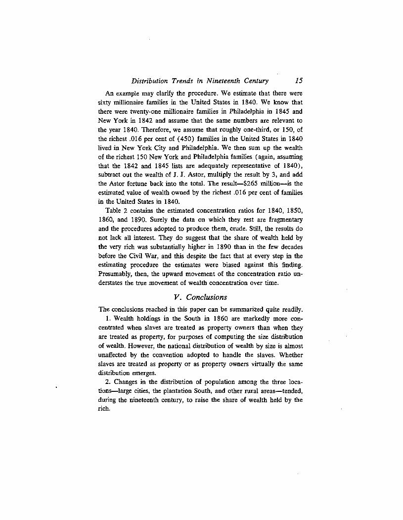
An example may clarify the procedure. We estimate that there weresixty millionaire families in the United States in 1840. We know thatthere were twenty-one millionaire families in Philadelphia in 1845 andNew York in 1842 and assume that the same numbers are relevant tothe year 1840. Therefore, we assume that roughly one-third, or 150, ofthe richest .016 per cent of (450) families in the United States in 1840lived in New York City and Philadelphia. We then sum up the wealthof the richest 150 New York and Philadelphia families (again, assumingthat the 1842 and 1845 lists are adequately representative of 1840),subtract out the wealth of J. J. Astor, multiply the result by 3, and addthe Astor fortune back into the total. The result—$265 million—is theestimate4 value of wealth owned by the richest .016 per cent of familiesin the United States in 1840.

Table 2 contains the estimated concentration ratios for 1840, 1850,1860, and 1890. Surely the data on which they rest are fragmentaryand the procedures adopted to produce them, crude. Still, the results donot lack all interest. They do suggest that the share of wealth held bythe very rich was substantially higher in 1890 than in the few decadesbefore the Civil War, and this despite the fact that at every step in theestimating procedure the estimates were biased against this finding.Presumably, then, the upward movement of the concentration ratio un-derstates the true movement of wealth concentration over time.

V. ConclusionsThe conclusions reached in this paper can be summarized quite readily.

1. Wealth holdings in the South in 1860 are markedly more con-centrated when slaves are treated as property owners than when theyare treated as property, for purposes of computing the size distributionof wealth. However, the national distribution of wealth by size is almostunaffected by the convention adopted to handle the slaves. Whetherslaves are treated as property or as property owners virtually the same4istribution emerges.

2. Changes in the distribution of population among the three loca-tions—large cities, the plantation South, and other rural areas—tended,during the nineteenth century, to raise the share of wealth held by therich.


3. Changes in the relative levels of wealth-holdings per family inlarge cities and in the rest of the country probably tended to raise theshare of wealth held by the very rich between 1860 and the end of thecentury.

4. The effects of changes in the structure of population and wealth-holdings (2 and 3, above) appear to have been quite limited, exceptwith respect to the share of wealth held by the richest 1 per cent offamilies.

5. The effects of changes in the structure of population and wealth-holWngs might have been countered by changes in the wealth distribu-tions in large cities and in rural areas. However, direct evidence relatingto the holdings of the very rich suggests that, in fact, the share of wealthheld by this group rose between the two decades before the Civil Warand 1890.

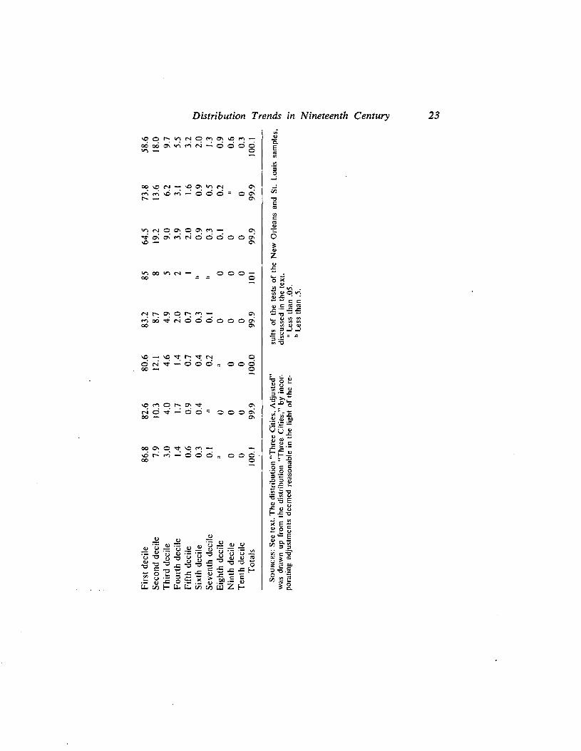
Appendix

WEALTH DATA IN THE MANUSCRIPT CENSUS

1850, 1860, 1870'°

Census enumerators were required to report the value of real propertyowned by respondents to the population questionnaire of the Census of1850. In 1860, and again in 1870, each respondent was to be asked thevalue of real property and the value of personal property he owned.The standard of valuation was to be gross market value. Personal prop-erty was to include intangibles and, consumer durables, but not clothing.Holdings of personal property of less than $100 were not to be enu-merated.1T

These data could have been tabulated by size of holding or by theresponse to any other question answered by the respondent; e.g., in1860, the age, sex, color, place of birth, marital status, occupation,family size and other family characteristics, place of residence, andmental or physical disability (if any) of the respondent. In fact, in 1850and 1870 they were not tabulated at all; in 1850, no doubt because the

16 The first six paragraphs of this appendix are taken, almost verbatim, fromRobert E. Galiman, "Social Distribution of Wealth in the United States ofAmerica," a paper delivered at the International Economic History Congress,Munich, 1965.

17 56th Congress, 1st Session, Senate Document No. 194, Washington, 1900,p. 157, instructions to enumerators in 1870.


Census Office lacked the resources to carry out the work; in 1870, forthe same reason and possibly because the Office doubted the value ofthe returns. In 1860 the returns were tabulated only by county and state.

In 1860 the census officials seem to have performed conscientiouslyand to have received the cooperation of respondents. At the very leastit can be said that the property return was not widely ignored or neg-lected. The aggregate value of property reported on the populationschedules exceeded the value of property assessed for tax purposes bymore than 50 per cent and the estimated true value of taxable property,by almost 20 per cent. Of course not all property was subject to tax,but on the other hand some of the property listed on the tax rolls be-longed to corporations and other institutions which were not enumeratedin the population census.18 Additionally, individuals owning personalproperty worth less than $100 were apparently not obliged to list theirproperty in the census but presumably were obligated to list for taxpurposes. Therefore, the large value of property reported on the popula-tion schedule, relative to the estimated true value of taxed property, isgood evidence that the enumerators and respondents met their obliga-tions.

Most of the original census sheets have been preserved an. recordedon microfilm. The library of the University of North Carolina holdsmicrofilms of census returns for virtually the entire South and we havehad available to us two sets of samples drawn from the 1860 materials.The first consists of 1 per cent samples of the families in Baltimore,New Orleans, St. Louis, Maryland outside Baltimore, and Louisianaoutside New Orleans. The second is a sample of farm operators drawnfrom all counties producing at least 1,000 bales of cotton in 1860.

SAMPLES FOR BALTIMORE, NEW ORLEANS, ST. LOUIS,

MARYLAND (Ex BALTIMORE) AND LOUISIANA (Ex NEW ORLEANS)

The samples for the three cities and two states were drawn in thefollowing way: the first family in each sample was selected at randomfrom the first page of the census relating to the sampled region. Wethen selected every hundre4th family thereafter. The smallest sample is314, the largest, 496.

18 Some were, however. For example, one railroad was returned on the popula-tion schedule in South Carolina, complete with age and occupational designation("railroad"). See, also, the discussion of institutions below.


We carried out two chi square tests, relating to the distribution ofoccupied persons among industries and occupations. The test of indus-trial distribution gave no evidence against the hypothesis that the samples(Maryland, including Baltimore, and Louisiana, including New Orleans,the only samples for which these tests can be conducted) were properlydrawn from the appropriate universes; the test of the occupational dis-tribution showed that the samples could not have been properly drawn.But neither test can be taken very seriously. The industrial test involvedvery few classes and the failure of the occupational test can be ascribedto problems of classification. For example, in one case a chief cause offailure was that the sample contained too few sales clerks and too manyclerks. But examination of the census tabulation suggests very stronglythat the census personnel who gathered the occupational data for thepublished tables classified most persons who reported themselves asclerks in the group, sales clerks.

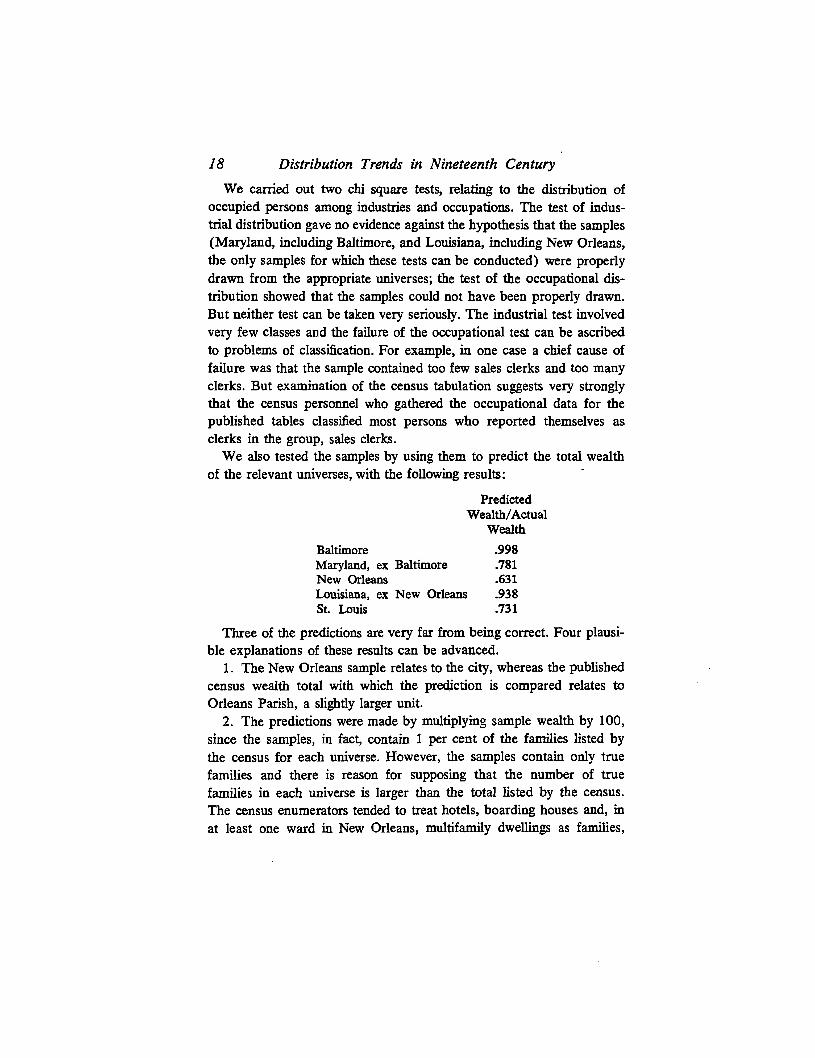
We also tested the samples by using them to predict the total wealthof the relevant universes, with the following results: -

PredictedWealth/Actual

Wealth

Baltimore .998Maryland, ex Baltimore .781New Orleans .631Louisiana, ex New Orleans .938St. Louis .731

Three of the predictions are very far from being correct. Four plausi-ble explanations of these results can be advanced.

1. The New Orleans sample relates to the city, whereas the publishedcensus wealth total with which the prediction is compared relates toOrleans Parish, a slightly larger unit.

2. The predictions were made by multiplying sample wealth by 100,since the samples, in fact, contain 1 per cent of the families listed bythe census for each universe. However, the samples contain only truefamilies and there is reason for supposing that the number of truefamilies in each universe is larger than the total listed by the census.The census enumerators tended to treat hotels, boarding houses and, inat least one ward in New Orleans, multifamily dwellings as families,


rather than enumerating separately the families living in these dwellings.Consequently, our estimating multipliers are too small.19

3. The census was apparently intended to collect data on wealthowned by natural persons and we have treated the reported totals asthough that intent had been realized. However, some institutionallyowned property was, in fact, listed on the schedules. For example, wefound property owned by convents on the Maryland schedules.

4. Wealth is very unequally distributed among the rich in the sampledregions and the samples are very small. Therefore, it is not likely thatthe samples accurately represent the average wealth-holdings of the veryrich. Furthermore, it seems more likely that the samples understate theholdings of the rich, than that they overstate them. This proposition issubject to test. Additionally, it is possible to obtain an impression ofthe extent to which the failure of the samples to represent the rich dis-torts the size distributions computed from the samples.

We focus on wealth owne4 by household heads and their spouses,for reasons that should be evident. In any event, household heads andtheir spouses owned most of the sampled wealth: 90.4 per cent in NewOrleans, 94.7 per cent in St. Louis, 83.6 per cent in Baltimore, 95.9per cent in Maryland, outside Baltimore, and 98.6 per cent in Louisiana,outside New Orleans. The principal test relates to New Orleans, sincethe wealth prediction made on the basis of the New Orleans sample wasleast satisfactory and, therefore, the New Orleans sample appears mostin need of testing. Finally, the test is conducted with data on the wealthholdings of the richest 900 od household heads in New Orleans. Ideallythe data would include wealth of spouses, but the omission appears tobe empirically unimportant. For convenience we refer to all wealth dataas "family wealth," although the reader should be aware that the meas-ures are imperfect representations of "family wealth." Measures cal-culated from the test data will be referred to as measures relating tothe "Universe," since the test data exhaust the classes of the universe towhich they refer. The published census total of all families will be treated

On the other hand, our samples surely do not adequately represent familiesliving in multifamily dwellings. Presumably the wealth holdings of these familieswere relatively small and therefore the samples may overstate average familywealth, compensating in some measure for the fact that the multipliers are toosmall.


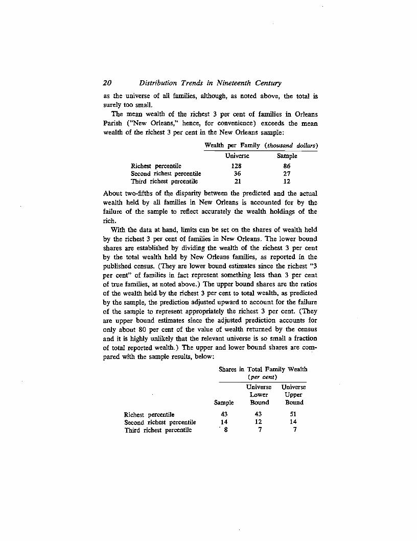
as the universe of all families, although, as noted above, the total issurely too small.

The mean wealth of the richest 3 per cent of families in OrleansParish ("New Orleans," hence, for convenience) exceeds the meanwealth of the richest 3 per cent in the New Orleans sample:

Wealth per Family (thousand dollars)Universe Sample

Richest percentile 128 86Second richest percentile 36 27Third richest percentile 21 12

About two-fifths of the disparity between the predicted and the actualwealth held by all families in New Orleans is accounted for by thefailure of the sample to reflect accurately the wealth holdings of therich.

With the data at hand, limits can be set on the shares of wealth heldby the richest 3 per cent of families in New Orleans. The lower boundshares are established by dividing the wealth of the richest 3 per centby the total wealth held by New Orleans families, as reported in thepublished census. (They are lower bound estimates since the richest "3per cent" of families in fact represent something less than 3 per centof true families, as noted above.) The upper bound shares are the ratiosof the wealth held by the richest 3 per cent to total wealth, as predictedby the sample, the prediction adjusted upward to account for the failureof the sample to represent appropriately the richest 3 per cent. (Theyare upper bound estimates since the adjusted prediction accounts foronly about 80 per cent of the value of wealth returned by the censusand it is highly unlikely that the relevant universe is so small a fractionof total reported wealth.) The upper and lower bound shares are com-pared with the sample results, below:

Shares in Total Family Wealth(per cent)

Universe UniverseLower Upper

Sample Bound Bound

Richest percentile 43 43 51

Second richest percentile 14 12 14Third richest percentile 8 7 7


The failings of the sample distribution are very nearly confined to therepresentation of the richest 1 per cent, and even here they are not veryserious, in terms of the requirements of this paper.

A simpler, less comprehensive, but perhaps as successful a test wasconducted with the St. Louis sample. The richest 1 per cent of thesample was blown up to represent the universe and the richest twenty-five families in the universe (those with $500,000 of wealth or more)were appropriately substituted into the group. When the prediction oftotal wealth derived from the sample is adjusted to reflect this change,the prediction accounts for 90.3 per cent of the wealth reported in thepublished census.

Maximum and minimum shares of wealth held by the richest 1 percent were also calculated, as in the New Orleans case, and the rangeturned out to be very narrow. The range falls above the value obtainedfrom the sample, but lies within the range obtained from the sample forNew Orleans, and not markedly above the sample value for Baltimore:

Shares iii Total Family Wealth (per cent)

St. Louis Universe

St. Louis Lower Upper BaltimoreSample Bound Bound Sample

Richest percentile 38 46 48 39

These results are encouraging, since we are interested in this paperchiefly in rural-urban differentials the findings suggest that the sam-ples are capable of revealing these differentials. For example, the threerural samples show the following shares of wealth held by the richest1 per cent:

Maryland, Louisiana, Cottoncx Baltimore cx New Orleans Counties

16% 24% 17%

Reasoning from the results of the tests of the urban samples, describedabove, the share of the richest 1 per cent of wealth-holders in Maryland(ex Baltimore) computed from the sample may understate the share ofwealth held by the equivalent group in the universe. But the margin forerror is surely not so great as to bring into question the existence of asubstantial difference between the share of wealth held by the richest 1

APP

EN

DIX

TA

BL

E A

-I

DIS

TR

IHU

TIO

NO

F G

RO

SS

WE

ALT

H A

MO

NG

FA

MIL

IES

, AC

CO

RD

ING

TO

SA

MP

LES

DR

AW

N F

RO

M T

HE

MA

NU

SC

RIP

TC

EN

SU

S O

F 1

860

FO

R B

ALT

IMO

RE

, NE

W O

RLE

AN

S, S

T. L

OU

IS, M

AR

YLA

ND

(E

x B

ALT

IMO

RE

), L

OU

ISIA

NA

(Ex

NE

W O

RLE

AN

S),

AN

D T

HE

CO

TT

ON

CO

UN

TIE

S(p

c,(c

liiof

gro

ss w

ealth

hel

d)

Thr

eeC

ities

,M

ary-

land

(cx

Lou

isi-

ana

(cx

Bal

ti-N

ewSt

.T

hree

Ad-

Bal

ti-N

ewC

otto

nFa

mili

esm

ore

Orl

eans

Lou

isC

ities

just

edm

ore)

Orl

eans

)C

ount

ies

'.4 IFi

rst (

rich

est)

per

cent

ile38

.543

.037

.639

.645

16.2

23.8

16.6

Seco

nd p

erce

ntile

15.0

13.6

12.6

13.1

129.

613

.58.

8T

hird

per

cent

ile7.

37.

79.

06.

96

7.6

7.7

6.5

Four

th p

erce

ntile

6.0

4.1

4.6

6.8

66.

57.

55.

5Fi

fth

perc

entil

e4.

93.

23.

94.

14

5.5

5.0

4.6

Sixt

h pe

rcen

tile

3.6

2.9

3.7

3.8

4•

4,7

4.0

4.1

Seve

nth

perc

entil

e3.

52.

22.

83.

03

4.1

3.6

3.6

Eig

hth

perc

entil

e3.

32.

22.

32.

42

3.7

3.0

3.2

Nin

th p

erce

ntile

2.7

2.1

2.3

2.3

23.

42.

93.

0T

enth

per

cent

ile2.

01.

61.

81.

2I

3.2

2.8

2.7

Firs

t dec

ile86

.882

.680

.683

.285

64.5

73.8

58.6

Seco

ndde

cile

7.9

10.3

12.1

8.7

819

.213

.618

.0T

hird

deci

le3.

04.

04.

64.

95

9.0

6.2

9.7

Four

th d

ecile

1.4

1.7

1.4

2.0

23.

93.

15.

5Fi

fth

deci

le0.

60.

90.

70.

7I

2.0

1.6

3.2

Sixt

h de

cile

0.3

0.4

0.4

0.3

0.9

0.9

2.0

Sev

enth

deci

le0.

1a

0.2

0.1

"0.

30.

51.

3

Eig

hth

deci

le0

00

0.1

0.2

0.9

Nin

th d

ecile

00

00

00

a0.

6T

enth

deci

le0

00

00

00

0.3

Tot

als

100.

199

.910

0.0

99.9

101

99.9

99.9

100.

1

SouR

cEs:

See

text

. The

dis

trib

utio

n "T

hree

Citi

es, A

djus

ted"

suIt

s of

the

test

s of

the

New

Orl

eans

and

St.

Lou

is s

ampl

es,

was

dra

wn

up f

rom

the

dist

ribu

tion

"Thr

ee C

ities

," b

y in

cor-

disc

usse

d in

the

text

.po

ratin

g ad

just

men

ts d

eem

ed r

easo

nabl

e in

the

light

of

the

re-

Less

than

.05.

Les

s th

an .5

.

-4 -4 -4 t'J


per cent in rural Maryland and the share of wealth held by the samegroup in the three urban areas.2°

SAMPLE FOR THE COTTON COUNTIES

The cotton counties sample is a sample of 5,229 farm operators 21(taken in clusters of approximately five) drawn from the manuscriptcensus records relating to counties that produced at least 1,000 bales ofcotton in the year 1860. (The counties involve4 produced 98 per centof U. S. cotton in that year.) The wealth covered by the sample con-sists of the personal wealth held by farm operators and the value of thefarms that they operated.22 Therefore, the sample excludes the value ofnonfarm real estate owned by farm operators and may, additionally,attribute the ownership of rental farm property to tenants, rather thanowners, although the latter is by no means certain.28 Consequently, werethe sample in all other respects adequate, we would suppose that the

20 For example, if the entire difference between predicted total wealth inMaryland (ex Baltimore) and the census return of wealth is attributed to samplingerror with respect to the richest 1 per cent, the holdings of that group can beinflated to 34 per cent of total wealth in Maryland (ex Baltimore). But obviouslythis assumption is extreme and therefore it is safe to assume that the share ofwealth held by this group is well below 34 per cent and, therefore, well belowthe share of urban wealth held by the richest 1 per cent of city dwellers.

21 The sample contains data drawn from the agricultural, free population,and slave schedules of the census. The first step in the sampling procedurewas the selection of farms from the agricultural schedule. We then moved tothe population schedule to find the farm owner. When it was discovered thatthe operator owned more than one farm in the sampled region, his farmingproperties were combined and treated as one property. This is the basis of theassertion that the sample is a sample of "farm operators." As will be evidentto the reader, the statement is not precisely accurate, since, presumably, someof the units in the sample consist of farms jointly operated, e.g., by a fatherand son. Very rarely, however, does the census attribute the operation of a farmto more than one person.

22 This statement requires qualification in two ways. First, the sample wastaken by states. Where a farmer operated more than one farm in a given state,we aggregated his property, as footnote 21 indicates. But farm properties locatedin different states were not aggregated, even when they were held by one man.Second, the census schedule called for the return of the value of each farm. Butfor several farms in the sample, the entry was not made. We suppose that inthese instances the farm was rented and that the value of the farm was notlisted on the schedules either because the respondent (the tenant) was regardedas an improper source of information relating to this question or because theenumerator regarded the question as one pertaining to the respondent and, there-fore, the entry of the relevant value in the schedule would constitute an incorrectattribution of property to the respondent.

23 footnote 22.


size distribution of wealth computed from the sample would understatethe degree of inequality of the distribution of wealth among farm opera-tors. However, our tests suggest that operators of large farm propertiesare somewhat overrepresented in the sample, compensating, at least insome measure, for the characteristics of the sample that tend to minimizewealth

COMMENTLEE SOLTOW, Ohio University

1. Professor Gailman has constructed very interesting wealth distri-butions for the urban and rural sectors and a composite for the UnitedStates in 1860. His findings, particularly for holdings of the rich in theurban and rural sectors, may prove to be close to those of a nationalsample covering all areas of the country. The amazing thing about thedistributions is the evidence of great inequality at such an early stage ofdevelopment. It would be of interest to know how this might havehappened in a land of opportunity.

2. I should like to confine my remarks to the conclusions of thepaper. The first is the finding that inclusion or exclusion of slaves in the1860 distribution does not really change the figures in the national dis-tribution. It is difficult to understand. this point other than to say that thenumber of slaves, as a per cent of the total population, was small andthat inclusion of these propertyless in the lower dediles of propertylesswould not matter. I certainly see why Professor Gailman used the ex-pedient of including slaves as having no wealth. But is this not a rathercallous way of looking at a human problem? Slavery is the ownershipof human bodies where a few slaveholders at the top of the distributionown many at the bottom of the distribution and the poor at the bottomdo not even own themselves. There were 4 million slaves valued at per-haps $4 billion or 15 to 20 per cent of our national assets. In taking $4

tests of the sample are described in Efficiency and Farm Interdependencein an Agricultural Export Region—Sampling Procedure and Tests of the Sample,'University of North Carolina, October 20, 1965; the results of the principal testsare described in James Foust and Dale Swan, "Productivity of Antebellum SlaveLabor—A Micro Approach," a paper given before the University of ChicagoWorkshop in Economic History, February 1967.


bfflion from the rich, should we not also give it to the poor as the priceof freedom?

I sometimes think this problem is best seen in terms of bodies. Let melargely confine myself to adult males, age 20 and up. There were threegroups in the United States: 400,000 who owned an average of tenslaves plus their own bodies; the large number of 6,600,000 adult malesowning their own bodies but no slaves; and 800,000 to 900,000 adultmale slaves owning nothing. Knowing the slave distribution, one cannow compute the Gini concentration coefficient of slaveholders, slave-holders plus nonslaveholders, and all adult males. The addition of thelast group increases concentration 20 per cent. One can go beyondbodies and use the census figures plus human-freedom valuations tocalculate the effect of slavery. A 10 to 20 per cent difference in theconcentration coefficient, plausibly, can be demonstrated, depending onthe amount of dollar weight attached to freedom.

The whole concept may break down unless one starts with a valuationof human as well as material wealth. In Adams County, Mississippi,which includes Natchez, the dollar wealth values declared in the 1860census give a Gini concentration coefficient of .91 for nonslave adultmales. If one includes adult male slaves at zero dollars, the coefficientincreases to .98. In 1870, all adult males in the county had a coefficientof .96 using the usual dollar calculation. It would certainly seem to be amockery of emancipation to speak of wealth concentration as decreasingonly from .98 to .96.

3. Professor Gallman's second, third, and fourth points deal with amodel explaining how wealth inequality may have increased from 1860to 1890. Since concentration in 1860 was greater in the urban sectorthan in the rural, and since the population moved, relatively, from therural to the urban sector, the concentration must have increased. Theargument is powerful. Where can one possibly find the counterpart tothe valuation of fifty acres when one lives in a city?

But the urban-rural dichotomy is only one aspect of the problem ofpopulation movement. There are, for example, age-nativity considera-tions. If the concentration among foreign born in 1860 was greater thanthat of native born, and the per cent of foreign born decreased after1860, one might expect the concentration to decrease. The averagewealth of native born was three to four times that of foreign born in


1860. The per cent foreign born in the ten largest cities in 1860 de-creased from 40 per cent in 1860 to 30 per cent in 1900. A city likeMilwaukee had a population in which 80 per cent of its adult maleswere foreign born in 1860, but only 53 per cent in 1900. There weregreat numbers of propertyless youths who were foreign born which de-creased relatively in the period. If, later, native-born groups began topredominate, homogenized by cultural institutions including educationand language, wealth in some broader sense than tangible property mighthave become less concentrated by the turn of the century.

4. One now turns to the actual data for 1840—1860 and the turn ofthe century. It can not be denied that a few thousand people owned atremendous share of total wealth in 1890 or 1900. But so did a few owna great share in 1860. A Pareto extrapolation of Gallman's 1860 Acurve shows .10 per cent holding the same wealth in 1860 as .03 percent did in 1890. His urban curve extrapolation shows the same per-centage holdings of the top .03 per cent in both years. Such differenceswould be rather meaningless on a Lorenz curve. If one goes further tothe share held by the top 9 per cent, he obtains a figure of 68 per centfrom Gallman's 1860 composite and 71 per cent from Holmes' 1890data. The interesting thing, it seems to me, is the extent of inequality in1860, not that it might have been minutely smaller than in 1890.

Professor Gailman found little effect from his urban-rural model andfelt his 1840—1890 estimates were crude and fragmentary. Perhaps weshould hold in abeyance any judgment about whether or not wealth in-equality increased in the last half of the last century until we have moreinformation. It is understood that the discussion pertains to wealthdistribution, not income distribution, and that it is very largely non-human wealth held by persons. Professor Galiman has presented an ex-tremely stimulating paper.

REPLYBY ROBERT E. GALLMAN

Since the meetings were held in March at Philadelphia two pieces ofevidence have come my way that tend to provide additional support forthe findings of my paper. Stanley Lebergott kindly sent me a pamphlet


published in the 1840's relating to the wealthy of Boston. (Our FirstMen, A Calendar of Wealth, Fashion and Gentility, Boston: Publishedby All Booksellers, 1846.) The pamphlet is similar to those producedby Moses Beach for New York. I have recomputed Table 2 of my paper,introducing the Boston evidence, and have obtained results virtuallyidentical to my original figures.

Table 1 of my paper contains wealth distributions for 1860 that wereestimated from sample evidence. An important assumption underlyingthe estimates was that the size distribution of weajth in the third, fifthand seventh largest cities in the U. S. in 1860 (the sample cities) wasrepresentative of the size distribution of wealth in the second throughtwentieth largest cities. (The precise cut-off point—i.e., the twentiethlargest city—is not very important. What is important is that the sampleevidence adequately represent large cities. See the fifth paragraph ofSection I of my paper.)

Taylor Cousins, of the University of North Carolina, has now shownme a wealth distribution he has derived for Richmond from an 1860census sample he has drawn. The distribution is very similar to the"three cities" distribution underlying Table 1 (see, also, Appendix TableA-i). Richmond was the twenty-fifth largest city in the U. S. in 1860.The finding lends support to my assumption that wealth was markedlyless equally distributed in cities than elsewhere.

I certainly have no quarrel with Professor Soltow's generous andthoughtful review of my paper. Soltow is right to underline the strikinginequality of wealth distribution before the Civil War, the limitedchanges in the distribution across time revealed by my estimating pro-cedures, and the desirability of working with more complicated modelsthan those I used. So far as the last point is concerned, the 1860 censusmaterials permit one to work with many potentially interesting variables(see the first page of the appendix).

There are two points relating to the institution of slavery, however,that call for some comment. First of all, the size distribution of wealthwithin the plantation South in 1860 is decidedly affected by the way inwhich slaves are regarded, as a comparison of the distributions containedin the notes to my text Table 1 ("Louisiana, ex New Orleans"; "CottonCounties") with those in Appendix Table A-i will show. When slavesare treated as potential property holders the distributions are very much


more unequal than when they are regarded as property. Professor Sol-tow's comments and examples tend to obscure this point.

It is the national distribution that is unaffected by the conventionadopted with respect to slaves and the explanation of this result lies notsimply in the limited fraction of the total population held in bondage in1860, as Professor Soltow suggests. If slaves are regarded as property,then the rich (i.e., the richest 1, 2, 3, etc. per cent) in the plantationSouth are far and away the wealthiest group in the nation and their hold-ings distend the wealth of those at the peak of the wealth pyramid. How-ever, if slaves are treated not as property, but as potential property hold-ers, the national distribution is affected in two ways. First, the averagehold,ing of the very rich falls markedly. However, now the population ofpotential wealth holders (families) is augmented by a substantial num-ber of families which, in fact, hold no wealth at all. These two changescompensate, at the national level, so that the various dedile groupings(percentile, within the richest decile) hold the same fraction of totalwealth when slaves are treated as potential wealth holders as when theyare regarded as property. (See the last paragraph of Section II of mypaper.)

The second point relates to Professor Soltow's proposal that thevalue of free men be included in aggregate wealth and the ownership ofeach free man's "body" be attributed to him. Soltow argues that such aprocedure would alter the wealth distributions, as well as the effect ofemancipation on the wealth distributions.

No doubt he is right, but one cannot be sure how important thesechanges would be. Soltow attempts one calculation. But it does not reallytell us what we want to know, since it is restricted to the distributionof ownership of human capital—indeed, to human capital implicit inand owned by males 20 years old or older—and rests on the assumptionthat all males 20 years and older are of equal economic value, an inde-fensible assumption.

Soltow also proposes that the matter of emancipation be dealt withby attributing wealth holdings to each slave equal to the price he wouldhave brought under slavery. But slave prices were formed under aplantation system run by compulsion. The freed slave's economic valuemight be more or less, under a tenant farm system or a plantation systemwith less power in the hands of the planter. Additionally, the slave sys-


tern limited the outlets open to slave workers. The freed slave, with hisfate in his own two hands, might find opportunities open to him whichcould not have been exploited under the slave system.

The last point should not be stressed unduly. Indeed, the selection ofwords used to make it draws attention to another difficulty with theSoltow proposal. How many freed slaves, now tenant farmers, really heldtheir fate in their own two hands after the Civil War? Soltow treats free-dom as absolute, but it is not. (My own handling of the problem is sub-ject to the same criticism.) The Negroes in the South simply weren't asfree, in any meaningful sense of the term, as western farmers, southernwhites, or northern factory workers.

Limitations on their freedom surely restricted the productive value offreed slaves. But there is more to it than that. Soltow hints that thevalue of a human to himself depends not only on production, but alsoconsumption criteria. Freedom has value to him. Then should not therestrictions on freedom suffered by the freed slaves be also taken intoaccount when Soltow's "human freedom valuations" are assigned? -

The point is not that Soltow's essential notions are inappropriate, butthat they involve more than Soltow was able to suggest in his brief re-marks.

Documents

Trends in the Size Distribution of Wealth in the ...piketty.pse.ens.fr/files/Gallman1969.pdf · the size distribution of wealth in the U. S. in 1860, following the ... of the Wealthy