Embed Size (px)
Citation preview

Exploring the Effect of Wealth Distribution on Efficiency Using a Model of Land Tenancy with Limited Liability
Nicholas Reynolds
Senior Thesis in Economics Haverford College
Advisor Richard Ball Spring 2011
Abstract
When perfect information is present in a model, the initial distribution of wealth will
have no effect on whether or not equilibrium is Pareto efficient. However, as Stiglitz (1987)
emphasized, this no longer holds when imperfect information is introduced: the initial
distribution of wealth can affect whether or not an economy is Pareto efficient. One reason, for
this effect is that the distribution of wealth can effect whether or not moral hazard, and the
inefficiencies associated with it, arise. In this paper, I demonstrate an example of this effect using
first a model of land tenure with limited liability found in Ray and Singh (2001) and then a
version of their model that is adapted by the addition of a second input into production. This
adaption allows me to demonstrate, under certain conditions, that the distribution of wealth not
only can affect whether or not the equilibrium allocation is first-best efficient but further whether
it is even constrained efficient.

Table of Contents
1. Introduction .......................................................................................... 1
2. Background and Literature Review .................................................... 4
3. Unadapted Model .............................................................................. 13
4. Model with Addition of Fertilizer ..................................................... 25
5. Caveats and Areas for Further Research ........................................... 42
6. Conclusion ........................................................................................ 47

1
1. Introduction
In neoclassical economic models with perfect information it is possible to prove that
issues of equity and efficiency can be treated separately. Specifically, it can be shown that
whether or not an economy is Pareto efficient does not depend on the initial distribution of
wealth. Thus, efficiency concerns are dealt with by focusing on correcting market failures, and
equity concerns are addressed by redistributing initial endowments and then letting the market
mechanism operate without any worry about the efficiency of the economy. However, as work
by Joseph Stiglitz and others in the economics of information has shown many of the basic
conclusions of the traditional neoclassical model do not hold when imperfect information, such
as asymmetric information between worker and capitalist, is introduced. For example, the
Fundamental Theorems of Welfare Economics do not hold: in general markets with imperfect
information are not Pareto efficient at equilibrium (Greenwald and Stiglitz, 1986). Further, the
separability of equity and efficiency no longer holds in general in economies with imperfect
information: whether or not an economy is Pareto efficient at equilibrium can depend on the
initial distribution of wealth.
This non-separability arises for a number of related reasons. In this paper, I will be
focusing on one specific reason. Asymmetric information between a lender and an investor,
between a landlord and a farm laborer, or between an insurer and an individual being insured can
lead to problems of moral hazard, which lead to inefficiencies. Importantly, the existence of the
above transactions and the moral hazard and inefficiencies associated with them can depend on
the distribution of wealth. Stiglitz (1987) writes, “The inefficiencies with which we have been
concerned arise because of the asymmetric information between two parties—between landlord

2
and worker, or between worker and capitalist. But whether these transactions arise is, at least
partly, determined by the distribution of wealth” (p. 16).
Sharecropping is a standard example used by Stiglitz and others to demonstrate this non-
separability. For example, he writes “The incentive problems associated with sharecropping
simply would not arise if all tenants owned the land upon which they worked” (p. 29). However,
Stiglitz, and others do not appear to have formally modeled how distribution affects efficiency
through its effect on the existence of moral hazard. There seem to be some difficulties with using
sharecropping, specifically a model of sharecropping such as that presented by Stiglitz (1974)
that focuses on risk-sharing, to formally model this effect. Thus in this paper I will use a model
of land-tenancy with risk-neutral tenants and limited liability constraints, meaning a tenant can
default if the payment is greater than their total wealth. In such a model, sharecropping does not
develop but moral hazard arises for tenants of certain wealth levels (Ray and Singh, 2001).
Using the Ray and Singh model and then a slightly adapted version I will be able to
demonstrate that the Pareto efficiency of the equilibrium allocation depends on the distribution
of wealth. I first use an unadapted version of the Ray and Singh model and then adapt it slightly
to obtain a stronger result, described below.
First, using a straight version of the Ray and Singh model I will demonstrate:
(1) that an equal distribution where all tenants have wealth above a certain cut-off level will
lead to an equilibrium that is first best Pareto efficient.

3
(2) that an unequal distribution where some tenants have wealth above a certain level and
some have wealth below that level will lead to an equilibrium allocation that is not first-
best Pareto efficient, but is constrained Pareto efficient1
Then, using an adapted version of the Ray and Singh model that includes a second input
in production (which can be understood as fertilizer), I will demonstrate the stronger conclusion
that distribution can affect the constrained Pareto efficiency of equilibrium, under certain
conditions. Specifically, I will show given certain conditions:
(1) that an equal distribution where all tenants have wealth above a certain cutoff level will
lead to an equilibrium that is first-best Pareto efficient
(2) that an unequal distribution with some tenants below the cut-off wealth slevel (and some
above it) will lead to an equilibrium that is not even constrained Pareto efficient, a simple
tax-and-subsidy scheme can lead to a Pareto improvement
Overall, I will demonstrate that in the presence of imperfect information whether or not
an equilibrium allocation is constrained Pareto efficient can depend on the distribution of wealth.
This is due to the fact that the existence of situations with moral hazard can depend on the
distribution of wealth.
This paper will begin with a review of relevant literature, starting with literature on the
effect of introducing imperfect information into economic models, then proceeding to a more
specific summary of literature related to the effect of moral hazard in sharecropping and land
tenancy. Following this will be a presentation of the Ray and Singh model, unadapted and then
1 If an allocation is first‐best efficient, even the introduction of perfect information would not represent a Pareto improvement. More weakly, if an allocation would be Pareto dominated by the perfect information equilibrium but there are no possible Pareto improvements taking the imperfect information as given than that allocation is constrained Pareto efficient. Finally, if there is a possible Pareto improvement to an allocation even taking the imperfect information into account, such as a tax‐and‐subsidy scheme, then the allocation is not even constrained Pareto efficient. The Greenwald and Stiglitz (1986) result described above demonstrated that with the presence of imperfect information the equilibrium allocation is not even constrained Pareto efficient under most circumstances.

4
with the addition of fertilizer, and a demonstration of the conclusions outlined above. Next, I will
describe some caveats and possible areas for further inquiry. Finally, I will conclude by
summarizing my findings and their implications.
2. Background and Literature Review
This paper draws primarily on literature in the fields of information economics and
development economics. As described above, information economics deals in general with the
effect that the introduction of imperfect information of various forms has on economic models
and their conclusions. This paper focuses on one type of inefficiency that arises from imperfect
information: moral hazard. Specifically, it deals with how the existence of moral hazard can
depend on the distribution of wealth. This analysis is carried out with an example from an
institution prevalent in developing countries: land tenure contracts. Thus, literature from
development economics, specifically that focusing on the form of rural institutions and
organizations, is relevant as well.
Information Economics
In combination the two fundamental theorems of welfare economics seem to provide an
almost impenetrable argument for the superiority of the market system as a way to allocate an
economy’s resources. If one is concerned about the efficiency of the economy, the First Theorem
tells us that the market mechanism will always lead to a Pareto efficient allocation in equilibrium,
and therefore that no one can be made better off without making at least one person worse off. If
one is still concerned with the equity of the allocation, whether the equilibrium allocation is fair
or just, the Second Theorem tells us that any Pareto efficient allocation can be achieved through
the market mechanism, all that needs to be changed are the initial endowments. In this traditional

5
story then concerns about efficiency and concerns about equity are separate. To ensure efficiency
a government just needs to allow the market to work and deal with limited market failures.
Separately, the government can make lump-sum transfers to obtain what society deems to be an
equitable distribution.
This traditional story works very well as long as the very specific assumptions of the
traditional neo-classical general equilibrium model hold. However, in many cases the
fundamental conclusions fail to hold when even minor changes are introduced. The relaxation of
the assumption of perfect information in particular leads many of the basic conclusions of the
neo-classical model, such as the law of one price and the Fundamental Theorems of Welfare
economics, to no longer hold (Stiglitz 1987).
Joseph Stiglitz, summarizing the contributions of information economics after its first
decade of existence, writes:
We have learned that much of what we believed before is of only limited validity; that the traditional competitive equilibrium analysis, though having the superficial appearance of generality—in terms of superscripts and subscripts—is indeed not very general; the theory is not robust to slight alterations in the informational assumptions. It is but a special—and not very plausible—‘example’ among the possible set of informational assumptions which can be employed to characterize an economy (Stiglitz 1985, p. 21).
For example, Greenwald and Stiglitz (1986) demonstrate that in general when imperfect
information is present the market equilibrium will not be Pareto efficient, simple tax-and-subsidy
schemes can in theory lead to Pareto improvements. This demonstrates not only that imperfect
information leads to inefficiencies in comparison to a world of perfect information, that the
equilibrium is not first-best efficient, but further that the equilibrium is not even Pareto efficient
taking the information problems is given, it is not even constrained Pareto efficient. This

6
conclusion demonstrates that with the introduction of imperfect information the First
Fundamental Theorem of Welfare Economics no longer holds in general.
Moral hazard is one of the most commonly studied ways that imperfect information can
lead to inefficiencies. Also known as hidden action, it refers to the fact that after a contract is
made, one party to the contract has an incentive to act in a way that will benefit themselves at the
expense of the other party (Collins dictionary of economics, 2006). With perfect information the
contract can include stipulations against such actions, but when information is imperfect one
party may not be able to observe all of the other’s actions and thus cannot enforce such
stipulations. A common example of moral hazard involves insurance. For example, if an
individual purchases fire insurance they will be more likely to take actions that increase the risk
of fire because they will not bear (all) of the costs of a possible fire. Moral hazard can arise in a
number of situations. For example, if worker has more information about their work effort than
their employer, they will incentive to not work as hard as they would if they were working for
themselves or if the employer had perfect information about their labor (Shapiro and Stiglitz,
1984).
(Non)-separability of Equity and Efficiency
Another conclusion of the perfect information model that fails to hold under more general
informational assumptions is the idea that issues of equity and efficiency are separable. What
exactly is meant by the separation of equity and efficiency, and thus what is meant if they cannot
be separated, is not always clear or consistent in the literature even among the same authors.
Often, it refers to the traditional story described above about the role of a theoretical government
in an economy. With perfect information, the fundamental theorems of welfare economics
demonstrate that concerns about efficiency and concerns about equity are completely separable
7
for a theoretical government. If a government is concerned that the particular Pareto efficient
allocation that exists at equilibrium is not socially-desirable, it can institute lump-sum transfers
to change the distribution of wealth. It can then allow the market to operate, confident in the fact
that the equilibrium that results will be Pareto efficient.
Most simply, this story breaks down with the introduction of imperfect information
because it is not feasible for a government to institute lump-sum transfers when information is
not perfect. If it is assumed that a government does not have perfect information about
individuals, it will not be able to costlessly determine what transfers it wishes to make. For
example, if a government wishes to enact redistributions to make wealth or income distribution
more equitable, it must design taxes that depend on wealth or income level. However, by
designing taxes to depend on some variable under individuals’ control, the government is
distorting incentives. The redistributions are no longer lump-sum transfers; they are distortionary.
Thus by making redistributions the government is now introducing distortions into the economy
that could affect efficiency. Efficiency and equity cannot be separated because attempts at
bringing about equitable or socially-desirable allocations will now have the potential to affect the
efficiency of those allocations (Stiglitz, 1985).
However, even if lump-sum transfers were possible, equity and efficiency would not be
separable with the presence of imperfect information. To understand why, it is useful to
introduce a related but slightly different way of understanding the separability of equity and
efficiency. Stiglitz (1985) writes, “One of the important consequences of the Fundamental
Theorem of Welfare Economics was that it enabled a neat separation of efficiency and equity
issues. In particular, whether the economy is or is not Pareto efficient did not depend on the
distribution of wealth” (15). This is another way of understanding the separation of equity and
8
efficiency. If the Pareto efficiency of equilibrium depends on the distribution of wealth, a
government’s attempts at achieving equity through even lump-sum redistribution could lead to
an equilibrium that is not Pareto efficient.
Stiglitz (1985) writes that with the introduction of imperfect information, whether or not
an economy is Pareto efficient can depend on the distribution of wealth. He refers to two reasons
that this can occur. First, in an economy with information problems that lead to inefficiencies,
the distribution of wealth determines whether it is feasible to design Pareto improvements, thus it
determines whether allocations are or are not constrained Pareto efficient. This result is
demonstrated formally in Shapiro and Stiglitz (1984). In a model of the labor market with
asymmetric information between workers and employers they demonstrate that the distribution
of the ownership of capital affects whether or not Pareto improvements can be designed.
Specifically, when it is assumed that ownership is distributed equally among all workers the
equilibrium is not constrained Pareto efficient, a tax and subsidy scheme can be designed that
leads to a Pareto improvement. However, when it is assumed that there are too distinct groups,
owners and workers, it is not possible to design a Pareto improving tax and subsidy scheme, and
thus the equilibrium is constrained Pareto efficient.
Αs Stiglitz explains, another reason that Pareto efficiency can depend on distribution is
that the existence of inefficiencies associated with imperfect information, such as moral hazard,
can depend on the distribution of wealth. If a worker has complete information about their work
effort, but that information is costly to his employer (for example a landowner or capitalist) there
will be added costs to the labor relations due to problems of moral hazard, either in the form of
decreased work effort by the worker or added monitoring costs for the employer. As Stiglitz
9
emphasizes whether these transactions and the inefficiencies associated with them arise “is, at
least partly determined by the distribution of wealth” (1985, p. 15).
In a number of articles Stiglitz uses the institution of sharecropping as an example. In
Stiglitz (1991) he writes, “The incentive problems associated with sharecropping simply would
not arise if all tenants owned the land upon which they worked” (p. 29). Similarly in Stiglitz
(1985), he writes “The moral hazard problems associated with sharecropping arise partly from
the fact that workers do not own the land upon which they work … More generally a basic
insight of the New New welfare economics is that whether the economy is or is not Pareto
efficient may depend on the initial distribution of wealth” (p. 31).
While Stiglitz frequently uses sharecropping as an example of the non-separability of
efficiency and distribution, he has not demonstrated the effect formally. When describing the
issue of equity and distribution he usually cites the result from Shapiro and Stiglitz (1984), which
as described above is a very different example from the sharecropping example: focusing on the
effect distribution has on the possibility of designing Pareto improvements rather than its effect
on the existence of moral hazard inefficiencies.
Land Tenure with Limited Liability
While the effect of distribution on efficiency is frequently referenced by Stiglitz, it is
usually as a side note, as part of the larger point that imperfect information changes many basic
results of neo-classical models. In contrast, Hoff (1996) and Bardhan, Bowles and Gintis (1999)
treat the effect of distribution on efficiency as the primary focus of their papers. Both present the
idea of using a model of land tenure with limited-liability constraints to examine issues of equity
and efficiency. In their models, which draw from earlier work by Shetty (1988), it is assumed
that there is some randomness in output based on weather and other conditions. Further, it is
10
assumed that there is an implied default clause in the contract, if the output is very bad and a
tenant does not have enough wealth to cover the fixed rent the tenant will default. Thus moral
hazard arises for tenants with wealth low enough to have a chance of default and these tenants
put out less than efficient levels of labor.
The use of limited-liability constraint models makes a lot of sense, in contrast with
Stiglitz’s risk-sharing model of sharecropping, because such a model more naturally
demonstrates the effect of distribution on the existence of incentive problems. Specifically, it is
clear directly from the model that whether or not moral hazard arises depends on a tenant’s
wealth level. Thus it seems to follow that the efficiency of the economy as a whole could depend
on the wealth distribution. However, Hoff and Bardhan, Bowles and Gintis do not focus their
analysis on the effect of distribution on Pareto efficiency specifically. Hoff focuses on the effect
that land redistribution could have on total output. Bardhan, Bowles and Gintis develop their
own concept of a “productivity enhancing redistribution” and demonstrate that such a
redistribution is possible in their model. The above authors demonstrate in a general sense that
equity and efficiency are not separable issues. However, they do not demonstrate the specific
claim made by Stiglitz: that wealth distribution can affect whether or not an economy is or is not
Pareto efficient through its effect on the existence of moral hazard.
Additionally, the above authors seem to suffer from a common mistake in the literature,
highlighted by Ray and Singh (1998), by assuming that a model with a limited-liability
constraint similar to Shetty (1988) can lead to sharecropping contracts. As Ray and Singh
demonstrate limited-liability similar to that first proposed by Shetty (1988) does not lead to the
existence of sharecropping. This error does not make limited-liability models any less useful for
11
the purpose of demonstrating the effect of wealth distribution on efficiency, but is an important
distinction.
As described above Ray and Singh demonstrate that limited-liability in a basic form is
not an explanation of sharecropping. However, their model can still be useful for the purpose of
demonstrating the effect of wealth distribution on efficiency because moral hazard still arises in
their model due to the limited-liability clause itself. Thus, I am able use their model to
demonstrate more formally Stiglitz’s assertion that whether or not an economy is Pareto efficient
depends on the distribution of wealth. This result occurs because whether or not moral hazard
occurs depends on the wealth level of the tenant.
However, Ray and Singh’s model only includes one good, labor, as an input for
production, which affects the ability to design Pareto improvements and thus affects the
constrained Pareto efficiency of equilibrium. This result mirrors earlier results of Stiglitz and
some of his coauthors. Specifically, in the Greenwald and Stiglitz (1986) result described above
it is only possible to design a Pareto-improving tax-and-subsidy scheme because there are
multiple goods interacting together. When there is only one good, no such Pareto improvements
are possible, so while the economy is not first-best Pareto efficient, it is constrained Pareto
efficient. Specifically, using the Ray and Singh model it is possible to demonstrate that some
distributions are first-best efficient and some are not, but all such distributions will lead to
equilibriums that are constrained Pareto efficient.
An example in Stiglitz (1994) was helpful in searching for a way to adapt the Ray and
Singh model to allow for Pareto improving tax-and-subsidy schemes. Stiglitz proposes a
situation where a sharecropper has two inputs, their labor and fertilizer which they purchase on
the market. Further he proposes that additional fertilizer use increases the marginal product of

12
labor. In such a situation, “the landlord benefits from the tenant’s use of fertilizer, not only
directly, through the increased direct yield, but also indirectly if the fertilizer increases the
marginal product of the tenant, and accordingly the tenant works harder” (p. 59). This is a
surprising result that only occurs because of the existence of imperfect information that leads to
moral hazard. Because moral hazard leads the tenant to undersupply labor, a subsidy on fertilizer
that increases the labor of the tenant will bring the labor level closer to the efficient level,
whereas if information was perfect the labor level would already be at the efficient level.
Given the Greenwald and Stiglitz result, introducing a second good of some kind seems
like it would allow for the demonstration of the stronger result, that distribution affects whether
or not an economy is constrained Pareto efficient. Combining this with the Stiglitz example of a
fertilizer subsidy, I chose to modify the Ray and Singh model by adding fertilizer as a second
input that increased the marginal product of labor. Given the literature cited above it seemed that
in such a model I would be able to demonstrate that when moral hazard occurred a Pareto
improving tax-and-subsidy scheme could be designed. Thus I would be able to demonstrate that
certain wealth distributions that did not lead to moral hazard would be Pareto efficient, while
distributions that led to moral hazard would not even be constrained Pareto efficient.
Overall, it appears that the literature is lacking a formal model that demonstrates the
effect, described by Stiglitz, that distribution has on Pareto efficiency through its effect on the
existence of relationships that bring about moral hazard. Thus in this paper I will use the Ray and
Singh model of land tenancy with limited liability constraints to demonstrate this effect. First, I
will use the unadapted model to demonstrate that wealth distribution affects whether or not an
economy is first-best Pareto efficient. Second, by introducing fertilizer into the model, I am able
to demonstrate the stronger conclusion. Using this model I demonstrate that under certain

13
conditions, whether or not an economy is constrained Pareto-efficient depends on the distribution
of wealth. Further, I outline specifically what conditions must hold for this to be the case.
3. Unadapted Model
Ray and Singh (1998)2 present a model of land tenancy with a limited liability constraint,
meaning that for “for sufficiently adverse realizations of output the rent cannot be paid
completely, the liability of the tenant is limited by his amount of wealth.” In other words if
particularly bad weather or other conditions lead to a bad harvest, the tenant may default on their
payments due. As emphasized by Shetty (1988), who formulated an earlier version of the model,
moral hazard problems similar to those found in sharecropping can arise in the presence of a
limited liability constraint, when default is possible. Importantly, as will be demonstrated in the
model, the existence of moral hazard and inefficient incentives depends on the wealth of the
tenant. I will present their model, and then use it to analyze the Pareto efficiency of different
distributions of wealth. As described above, I will demonstrate that in this model whether or not
an economy is first-best Pareto efficient can depend on the distribution of wealth.
Set-up of the Model
In the model both tenants and landlord are assumed to be risk neutral. The production
function representing a tenants production of crop is defined as )(LQQ , where Q’>0,
2 Ray and Singh present two variations of the model. In the first variation the cropshare, the share of
output that the tenant receives, is allowed to be greater than one. In this variation by pushing the cropshare above one contracts for less wealthy tenants can be pushed to efficiency by setting the cropshare greater than one. However, they present a number of reasons that it is reasonable to assume that in reality the cropshare would be constrained to be less than one. Thus, they present a second variation of the model with cropshare constrained, which results in the very different conclusions I describe. I will be using the second variation.

14
Q’’<0, 0, Q(L)=0, 3 and is a random variable with distribution function ],[, F .
represents the randomness in agricultural output due to weather and other circumstances. Let W
be the initial wealth of the tenant. Landlords are able to observe the wealth level of tenants.
Tenants and landlords are assumed to bargain over the form of the contract. It is assumed
further that landlords cannot determine the work effort of their tenants and that monitoring is too
costly to be implemented. Therefore contracts are limited to be either rental contracts or share
contracts, or some hybrid form in between. In the model it is assumed that tenants compete for
landlords, but as Ray and Singh emphasis the results would be the same if the reverse were
assumed. The tenant’s income from the contract is defined as CLQ )( , where is the
tenant’s crop-share, the proportion of output the tenant keeps as determined by the contract, and
C is the fixed rental component of the contract (when C is positive it represent the payment made
by the tenant to the landlord). Similarly, the tenants payment to the landlord is:
CLQ )()1( .
To represent the limited liability constraint 1 is defined as a value of such that the
tenant cannot make the agreed upon payment, defined above as CLQ )()1( , for any
value of less than or equal to 1 . In other words,
1 represents the weather and other
conditions that would lead to the tenant defaulting under those conditions or any worse
conditions. Formally 1 is defined as follows:
, , ; :
3 Ray and Singh do not include this explicitly as an assumption, but it is used (and necessary) later in their paper. It is also a very reasonable assumption: that if the tenant puts in no labor they will yield no output.
15
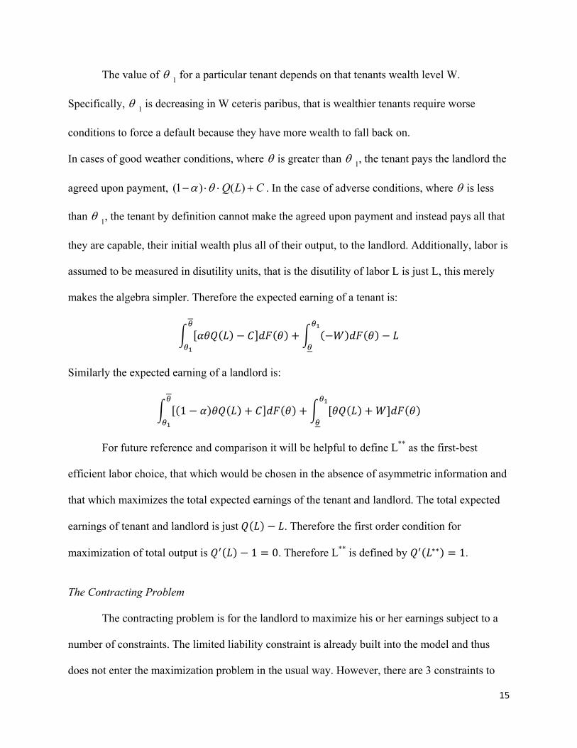
The value of 1 for a particular tenant depends on that tenants wealth level W.
Specifically, 1 is decreasing in W ceteris paribus, that is wealthier tenants require worse
conditions to force a default because they have more wealth to fall back on.
In cases of good weather conditions, where is greater than 1, the tenant pays the landlord the
agreed upon payment, CLQ )()1( . In the case of adverse conditions, where is less
than 1, the tenant by definition cannot make the agreed upon payment and instead pays all that
they are capable, their initial wealth plus all of their output, to the landlord. Additionally, labor is
assumed to be measured in disutility units, that is the disutility of labor L is just L, this merely
makes the algebra simpler. Therefore the expected earning of a tenant is:
Similarly the expected earning of a landlord is:
1
For future reference and comparison it will be helpful to define L** as the first-best
efficient labor choice, that which would be chosen in the absence of asymmetric information and
that which maximizes the total expected earnings of the tenant and landlord. The total expected
earnings of tenant and landlord is just . Therefore the first order condition for
maximization of total output is 1 0. Therefore L** is defined by 1.
The Contracting Problem
The contracting problem is for the landlord to maximize his or her earnings subject to a
number of constraints. The limited liability constraint is already built into the model and thus
does not enter the maximization problem in the usual way. However, there are 3 constraints to
16
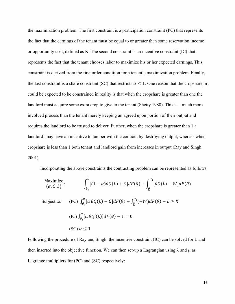
the maximization problem. The first constraint is a participation constraint (PC) that represents
the fact that the earnings of the tenant must be equal to or greater than some reservation income
or opportunity cost, defined as K. The second constraint is an incentive constraint (IC) that
represents the fact that the tenant chooses labor to maximize his or her expected earnings. This
constraint is derived from the first order condition for a tenant’s maximization problem. Finally,
the last constraint is a share constraint (SC) that restricts 1. One reason that the cropshare, ,
could be expected to be constrained in reality is that when the cropshare is greater than one the
landlord must acquire some extra crop to give to the tenant (Shetty 1988). This is a much more
involved process than the tenant merely keeping an agreed upon portion of their output and
requires the landlord to be trusted to deliver. Further, when the cropshare is greater than 1 a
landlord may have an incentive to tamper with the contract by destroying output, whereas when
cropshare is less than 1 both tenant and landlord gain from increases in output (Ray and Singh
2001).
Incorporating the above constraints the contracting problem can be represented as follows:
Maximize, , : 1
Subject to: (PC)
(IC) 1 0
(SC) 1
Following the procedure of Ray and Singh, the incentive constraint (IC) can be solved for L and
then inserted into the objective function. We can then set-up a Lagrangian using and as
Lagrange multipliers for (PC) and (SC) respectively:

17
, , , , 1 ·
· 1
The first order conditions for this Lagrangian are then as follows:
, , , , = 1 ′ ′
0
and
, , , , 0
At this point Ray and Singh consider three “exhaustive and mutually exclusive cases”
depending on which constraints bind. I will follow this method.
Case 1: Participation constraint does not bind
In this case we assume that the participation constraint (PC) does not bind. By definition
because (PC) does not bind =0. The first order condition for C then becomes:
, , , , 0
From this we can conclude that . In other words, the tenant will default under all
conditions. Given this fact, we return to the tenant’s maximization of his or her expected
earnings (by choosing L):
Given that , the above maximization becomes:

18
Given that L is constrained such that 0, the tenants maximizing labor choice will be:
L*=0. That is, to maximize his or her expected earning the tenant chooses to not put out any
effort, because his or her wealth level is so low that they will default under any circumstances.
Given that Q(L*)=0, the original definition of , , becomes W=C. That is,
the fixed rent is equal to the tenants wealth level.
Now given that the (PC) does not bind, , and L*=0, (PC) becomes:
Which simplifies to, – , or . Therefore in this case, the tenants wealth
level is less than (-K), in other words the tenant is indebted.
Finally, since the landlords expected earnings becomes:
1
Given that 0, and thus Q(L)=0, this simplifies to just W. From above we know that
, so the landlords expected earnings would be less than (-K). If the landlord did not
lease the plot at all and just left it fallow his expected earnings would be 0, which is greater than
(-K). Therefore it is the maximizing landlord’s interest not to rent the land at all. This result
arises because the landlord is so poor that they expect to default under any conditions and thus
have no incentive to put out any effort. In conclusion then, Case 1 is not a solution to the
contracting problem, no contract will arise and the landlord will leave the plot fallow.
Case 2: Participation constraint binds and 1

19
For this case we assume that the participation constraint (PC) binds as an equality and
that the cropshare constraint (CC) does not bind at equality, that is 1. By definition then,
0.
Given that the participation constraint (PC) binds we have:
It is clear that if , (PC) would become – . Because we have assumed
that 0, we would either have that the tenant is indebted or the above expression would be a
contradiction. Either way we can conclude that for this case to be a solution to the contracting
problem .
Now we can examine the first order condition for C:
, , , 0
Which we can rearrange to:
1 0
Given that , we can conclude that 0, and thus that 1. Therefore
the first-order condition for becomes:
, , , ,
1 ′ ′
0

20
After some rearranging this becomes:
′ 1 1 0
Using the incentive constraint (IC) we see that the second term is equal to zero and drops out.
We are thus left with:
1
which, given that 0 and 0, implies:
1
We know from the definition of the distribution of , that 1 . Therefore the above
equation tells us that 1, which is a contradiction given that the case under consideration
assumes that 1. Therefore this case does not arise as a solution to the contracting problem.
Together the fact that Case 1 and 2 lead to contradictions, demonstrates that situations where the
share constraint does not bind cannot be solutions to the contracting problem. A true share
contract (where the tenants share 1) will not arise in this model. If a solution does arise for
the final case it will be a fixed rent contract. This is one of the main conclusion of Ray and Singh:
that a limited liability constraint such as that used in their model cannot be an explanation for
sharecropping.
Case 3: Participation constraint binds and 1
In the third and final case we will assume that the participation constraint (PC) and
cropshare constraint (CC) both bind at equality. That is, 1, 0, and 0. As in Case 2,

21
it is evident from the first order condition for C that 1. Therefore the first order condition for
becomes:
, , , , = 1 ′ ′
0
With some rearranging and cancellation this becomes:
1
Given that 1, the incentive constraint (IC) becomes: 1 0. Thus the
first term is equal to zero and drops out, leaving:
Which implies that 0. This is not a contradiction with the assumptions of the case.
This case holds as a solution to the contracting problem. Thus we have shown that the only
solution to the contracting problem is a case where 1. In other words, in all contracts the
tenant will get to keep all of their output, no sharecropping will arise in this model. While we
have not yet shown the specific value of the fixed rent, C, it is clear that if the tenant is receiving
all of the output and the landlord is receiving none, there must be some fixed rent paid from the
tenant to the landlord. Following the strategy of Ray and Singh we will now examine two
subcases of Case 3 that will give us greater insight into effect that wealth level has on contract
form and efficiency.
Case 3(a): Participation constraint binds, 1, and limited liability constraint does not bind
In this sub-case we will assume as in Case 3 that the participation constraint (PC) and the
cropshare constraint (CC) both bind and equality. Further we will assume that the limited
22
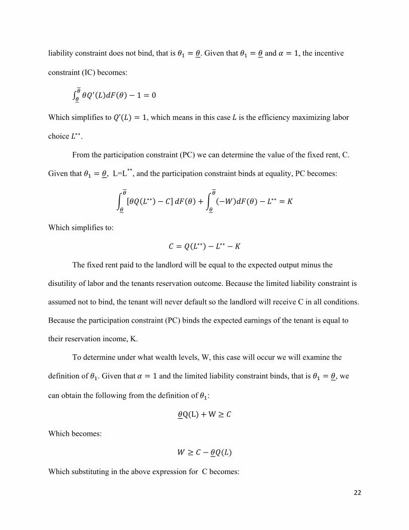
liability constraint does not bind, that is . Given that and 1, the incentive
constraint (IC) becomes:
1 0
Which simplifies to ’ 1, which means in this case is the efficiency maximizing labor
choice .
From the participation constraint (PC) we can determine the value of the fixed rent, C.
Given that , L=L**, and the participation constraint binds at equality, PC becomes:
Which simplifies to:
The fixed rent paid to the landlord will be equal to the expected output minus the
disutility of labor and the tenants reservation outcome. Because the limited liability constraint is
assumed not to bind, the tenant will never default so the landlord will receive C in all conditions.
Because the participation constraint (PC) binds the expected earnings of the tenant is equal to
their reservation income, K.
To determine under what wealth levels, W, this case will occur we will examine the
definition of . Given that 1 and the limited liability constraint binds, that is , we
can obtain the following from the definition of :
Q L W
Which becomes:
Which substituting in the above expression for C becomes:

23
We can thus define a cutoff level of wealth, , such that this case (Case 3a) will arise for
tenants with . Because of the earlier results of this case, this is also the cutoff level such
that tenants with will have contracts that lead them to put out the efficient labor level,
L**, and thus will lead to the maximization of total output, in other words first-best efficiency.
This cutoff level is defined as follows:
We will now proceed to the second sub-case.
Case 3(b): Participation Constraint Binds, 1, and Limited Liability Constraint Binds
In this sub-case we will assume as in Case 3 that the participation constraint (PC) and the
cropshare constraint (CC) both bind and equality. Further, in contrast to Case 3(a) we will
assume that the limited liability constraint does bind. In other words, the tenant’s wealth is low
enough that there is a chance of default under some conditions, formally, that is .
Given that 1 the incentive constraint (IC) becomes:
1 0
Which can be rearraned to give us:
1
Given the distribution of and the fact that , we can conclude that
1. Thus the above expressions tells us that 1. The tenant will not choose the efficient
labor level, . Given that Q L 0, it is clear that the tenant in this case will choose a labor

24
level below the efficient level, that is . The intuition behind this result is simple: in the
case of default the tenant does not receive any of the output and thus does not receive any benefit
from their labor input, therefore if a tenant has a low enough wealth level that there is some
chance of default they will not have incentives to choose a labor level that maximizes total
output. Thus in this case total output is not maximized due to moral hazard, the equilibrium
contract for less wealthy tenants is not first best efficient.
Welfare Analysis
Given the above analysis of contract forms under different wealth levels, it is possible to
execute a welfare analysis comparing the Pareto efficiency of different wealth distributions. I
will demonstrate that under Ray and Singh’s model the distribution of initial wealth affects the
first-best Pareto efficiency of equilibrium, but not the constrained efficiency. As described earlier
the model must be adapted to demonstrate the stronger result with constrained efficiency.
We will compare the welfare properties of two distributions, one where all tenants hold
equal wealth and one where wealth is distributed unequally. For both distributions, the total
number of tenants is equal to n and the total wealth of tenants is equal to , the number of
tenants times the cutoff wealth level. Under Distribution A, all tenants hold equal wealth, .
Under Distribution B tenants are split into two equal sized groups of tenants. The first group
has wealth, , where y is an arbitrary constant. The second group holds wealth,
.
First, consider the welfare properties of Distribution A. Because all tenants hold wealth at
least equal to , at equilibrium all contracts arising from this distribution will be of the form
demonstrated in Case 3(a). Therefore, all tenants will choose the efficient labor level, L**, that
25
maximizes total output for themselves and the landlord. All contracts will be first best efficient
and therefore the equilibrium will be first-best Pareto efficient.
Next, we can consider the welfare properties of Distribution B. The more wealthy tenants,
with , will receive contracts of the form demonstrated in Case 3(a), and will thus
put out the efficient labor level, L**, that maximizes total output for themselves and the landlord.
However, the less wealthy tenants, with , will receive contracts of the form
demonstrated in Case 3(b). Therefore, they will choose a level of labor less than that the efficient
level, that is , the total welfare of tenant and landlord will not be maximized at a first-
best level. These contracts will then not be first-best efficient. We can then say that the
equilibrium of the economy overall is not first best efficient.
Thus, we have the result that the initial distribution of wealth affects whether or not the
equilibrium is first-best Pareto efficient. For one distribution, the equilibrium is first best
efficient because no moral hazard occurs, and for another distribution the equilibrium is not first-
best efficient because of the existence of moral hazard. However, both distributions are
constrained Pareto efficient, taking the imperfect information as given no Pareto improvements
are possible. In the following section I attempt to adapt the Ray and Singh model slightly to
obtain the stronger result, that the constrained Pareto efficiency of equilibrium depends on the
initial distribution of wealth.
4. Model with Addition of Fertilizer
I will now present a version of the Ray and Singh model that is adapted by the addition of
a second input in the production function. This additional input can be understood as fertilizer. In
this model, a tenant chooses not just an amount of labor but also can purchase fertilizer on the

26
market and use it on the fields. Additional fertilizer is assumed to increase output and also to
increase the marginal productivity of labor. If a tenant uses more fertilizer it not only directly
increases output, but also makes their labor more productive. This assumption is important
because it will eventually allow for a subsidy on fertilizer that will not only lead a tenant to use
more fertilizer but will also indirectly lead to the tenant choosing to put out more labor.
Just as labor was assumed to not be observable to the landlord, the amount of fertilizer
that a tenant uses is also unobservable to the landlord. While the landlord could more easily
observe or mandate how much fertilizer is purchased, it would be difficult for the landlord to
ensure that the tenant actually used the fertilizer and did not sell it back on the market. In most
other respects the model is the same as Ray and Singh, as shown below.
Set-up of the Model
As in the earlier model tenants and landlords are assumed to be risk neutral. A tenant’s
output is defined as , , where L is labor, X is fertilizer and is a random variable
representing randomness in output due to weather and other factors. It is assumed that 0,
0, 0, 0, and 0. has distribution function F, , , and E( )=1.
Again, a tenant’s wealth level is defined by W, and landlords are able to observe a tenants wealth
level. The tenant’s income from the contract is defined as , . Similarly, the tenant’s
payment to the landlord is defined as 1 , . The tenant is assumed to have a
reservation income K. It is assumed that 0.
As before is defined as the value of such that the tenant cannot make the agreed
upon payment and will default when . Formally is defined as follows:
, , , ; : ,
,

27
Tenants are assumed to purchase fertilizer at a constant market price, , where 0. For
simplicity, it is assumed that a tenant always has enough wealth to purchase the amount of
fertilizer they choose to. However, it is assumed that the purchase of fertilizer takes place at the
beginning of the period and thus is subtracted from the wealth level left by the end of the period.
Therefore in the case of default the tenant pays to the landlord all their output plus their
remaining wealth subtracting the amount they spent on fertilizer. As will be examined further
this leads to an odd result where in the case of default the tenant experiences neither the benefit
nor the cost of fertilizer use. The effect of this “double moral hazard” on the tenant choice of
fertilizer is examined in more detail below.
Formally, the expected earning of the tenant is defined as follows:
,
Similarly the expected earning of the landlord is:
1 , ,
Again, we will define , and now additionally, as the first-best efficient labor and
fertilizer choices that maximize total expected earnings. Total expected earnings is:
,
Thus the maximization of expected earnings yields the following first order conditions for
maximization:
FOC (L): 1 0
FOC (X): 0
Therefore we can define and as those values that satisfy: , 1 and
, . Importantly, these two values come as a pair, that is for X and L to be at the

28
efficient level the pair of values of and must together satisfy both of the above conditions.
For example if , 1, but , neither fertilizer or labor are at the efficient level
or .
The Contracting Problem
As before the landlord maximizes his or her earnings subject to a number of constraints.
The participation constraint (PC) and share constraint (SC) are the same concept as above. With
the addition of fertilizer to the model there are now two incentive constraints, one for labor (ICL)
and one for fertilizer (ICX). These constraints are derived from the tenant’s maximization of his
earnings, as shown below:
, ,
The first order conditions for maximization are thus:
FOC(L): , 1 0
FOC(X): , 0
These become the two incentive constraints ICL and ICX respectively. Thus the contracting
problem can be represented by the landlord’s maximization subject to constraints as follows:
, 1 , ,
Subject to:
(PC) ,
(ICL) , 1 0

29
(ICX) , 0
(CC) 1
Following Ray and Singh the incentive constraints (ICL) and (ICX) are solved for L and
X respectively and substituted into the objective function. The remaining constraints can be
incorporated into the maximization through a Lagrangian. The Lagrangian, with and as
Lagrange multiplier for (PC) and (SC) respectively, is below:
, , , 1 , ,
, 1
The first-order conditions for the Lagrangian, in terms of and are thus:
, , , , 1
,
0
, , , 0
As above, now that the basic contracting problem is established we can examine three
cases, with different assumptions about which constraints bind. As before Case 1, in which the
participation constraint (PC) is assumed not to bind, does not hold as a solution to the contracting
30
problem. The reasoning for this result is the same as for the unadapted model, and is
demonstrated formally in an appendix.
However, the addition of fertilizer, and specifically the different way that limited-liability
affects fertilizer, leads to the result that Case 2 and Case 3 can both hold under different
conditions. In Case 2 the participation constraint is assumed to bind but the share constraint is
assumed not to bind, that is α 1. In Case 3 the participation constraint is again assumed to bind
and the share constraint is also assumed to bind, that is 1. Thus the fact that Case 2 and Case
3 can hold, demonstrates that sharecropping will arise under certain conditions and not arise
under others. This is in contrast to the result of Ray and Singh outlined above for a model
without fertilizer, that only Case 3 can hold and thus no sharecropping will arise.
This is an interesting result and brings back on the table the possibility of limited-liability
as an explanation for sharecropping. However, to demonstrate the effect that is the focus of this
paper, that the constrained Pareto-efficiency of equilibrium can depend on the distribution of
wealth, I will proceed by assuming that Case 3 holds, and thus 1 and no sharecropping
arises. A brief examination of the conditions that cause each case to hold is left to a later section
on caveats and areas for further research.
Case 3: participation constraint binds, cropshare constraint binds
We assume that Case 3 binds, thus the participation constraint (PC) and the cropshare
constraint (CC) bind. Now we proceed to examine the different results of this case depending on
whether or not the limited-liability constraint binds.
Case 3(a): Participation constraint binds, share constraint does not bind, limited liability
constraint does not bind
31
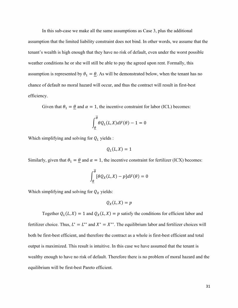
In this sub-case we make all the same assumptions as Case 3, plus the additional
assumption that the limited liability constraint does not bind. In other words, we assume that the
tenant’s wealth is high enough that they have no risk of default, even under the worst possible
weather conditions he or she will still be able to pay the agreed upon rent. Formally, this
assumption is represented by . As will be demonstrated below, when the tenant has no
chance of default no moral hazard will occur, and thus the contract will result in first-best
efficiency.
Given that and 1, the incentive constraint for labor (ICL) becomes:
, 1 0
Which simplifying and solving for yields :
, 1
Similarly, given that and 1, the incentive constraint for fertilizer (ICX) becomes:
, 0
Which simplifying and solving for yields:
,
Together , 1 and , satisfy the conditions for efficient labor and
fertilizer choice. Thus, and . The equilibrium labor and fertilizer choices will
both be first-best efficient, and therefore the contract as a whole is first-best efficient and total
output is maximized. This result is intuitive. In this case we have assumed that the tenant is
wealthy enough to have no risk of default. Therefore there is no problem of moral hazard and the
equilibrium will be first-best Pareto efficient.

32
As before, we can define formally a cutoff wealth level above which this case will occur.
In other words, we can define how wealthy a tenant must be to have no chance of default and
therefore have a contract that leads to first-best efficiency. This is a multi-step process: I will
begin by using the participation constraint (PC) to define a value of C, then I will use the
definition of to obtain an expression of W, and finally I will substitute the expression for C
into the expression of W.
First examine the participation constraint (PC) given that :
,
Which simplifies to:
,
Which solving for W yields:
,
Now we will examine the definition of , in order to obtain an expression for W. Given
that 1, , and , the definition of becomes:
,
Solving for C this becomes:
,
Substituting the expression for C obtained above this becomes:
, ,
We can define a cutoff level , such that this case only occurs if . Given the above
expression we define as:
, ,

33
Tenants with will have no chance of default, and thus no moral hazard will arise in their
contracts. Therefore for these tenants and their landlords (as in the unadapted model) the
equilibrium will be first-best Pareto efficient, it will maximize total output.
For the welfare analysis below it will be helpful to have an expression of the landlord’s
expected earnings for this case. Given that and 1, the expression for the landlord’s
expected earning’s becomes:
,
Which simplifies to just . Thus the tenants expected earnings is equal to the expression above
for C, which is:
,
Case 3(b): Participation constraint binds, share constraint does not bind, limited liability
constraint does bind
For this case we will assume as in Case 3 that the participation constraint (PC) and the
share constraint (SC) both bind at equality. Additionally, we will assume that the limited liability
constraint does not bind, that is the tenant’s wealth is low enough that he or she has a chance of
defaulting under some adverse conditions. Formally, that is . As I will show, in this case,
as in the unadapted model, equilibrium will not be efficient because having some probability of
default leads to moral hazard and thus an inefficient choice of labor and fertilizer.
First we examine the incentive constraint for labor (ICL), given that 1:
, 1 0
This can be solved for , yielding the following expression:

34
,1
Given that 1, this implies that , 1. Thus . As in the
unadapted model, in this case the tenant will undersupply labor. Under certain conditions the
tenant will default and not receive any benefit of labor, but will still have to bear the cost of labor
disutility. Thus the choice of labor that maximizes the tenants output is lower than the choice of
labor that would maximize total output.
Now we can examine the incentive constraint for fertilizer (ICX), given that 1:
, 0
Solving this for yields:
, ·
It can be demonstrated that when . Thus 1
and the above expression implies that . This implies that the tenant will oversupply
fertilizer, that . This is an interesting result that arises because of the “double moral
hazard” effect on fertilizer, where in the case of default the tenant experiences neither the benefit
nor the loss from additional fertilizer use.
The intuition behind this result is somewhat complex. At first blush it may seem
reasonable to assume that the two moral hazard-like effects would cancel out, and fertilizer
choice would be efficient, but this does not turn out to be the case. The result that fertilizer is
oversupplied depends on the fact that conditions that lead to default, where the tenant does not
35
care what level of fertilizer they supply, occur for low values of . On the other hand, when the
tenant’s choice of fertilizer does affect them, the values of will be higher. Thus, the marginal
product of fertilizer is higher for the cases where the tenant will not default, than the average
marginal product of fertilizer for all cases. Since, the tenant chooses their fertilizer uses based on
these cases they will oversupply fertilizer, compared to the efficient level of fertilizer that would
maximize total output.
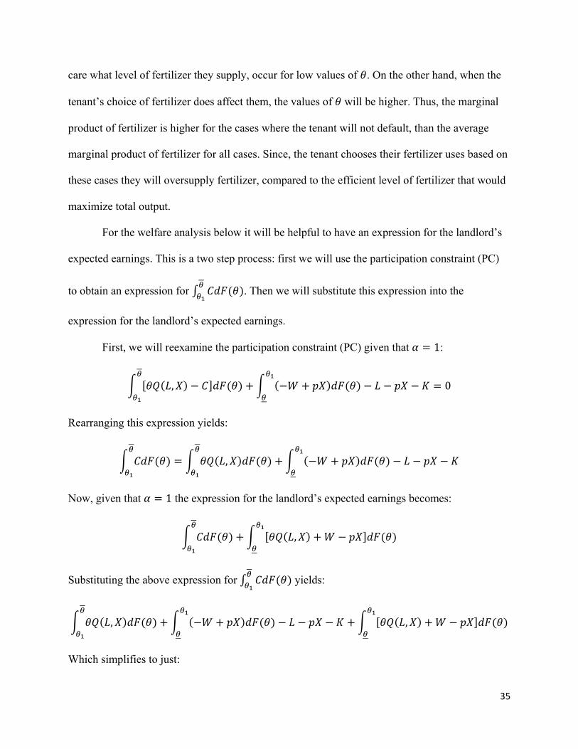
For the welfare analysis below it will be helpful to have an expression for the landlord’s
expected earnings. This is a two step process: first we will use the participation constraint (PC)
to obtain an expression for . Then we will substitute this expression into the
expression for the landlord’s expected earnings.
First, we will reexamine the participation constraint (PC) given that 1:
, 0
Rearranging this expression yields:
,
Now, given that 1 the expression for the landlord’s expected earnings becomes:
,
Substituting the above expression for yields:
, ,
Which simplifies to just:

36
,
This is the same expression as above in Case 3(a), except the values for L and K are not the
optimal levels L** and K** as above.
Welfare Analysis
As before, for the unadapted Ray and Singh model, now that we have analyzed contract
forms under different wealth levels, it is possible to execute a welfare analysis comparing the
Pareto efficiency of different wealth distributions. I will demonstrate that under the adapted
model the distribution of initial wealth can be shown under certain conditions to affect not only
the first-best Pareto efficiency of equilibrium but also the constrained Pareto efficiency.
Again, we will compare the welfare properties of two distributions, one where all tenants
hold equal wealth and one where wealth is held unequally. The distributions to be compared are
the same as above. There are assumed to be n tenants in both distributions. Under Distribution A,
all tenants hold equal wealth, . Under Distribution B tenants are split into two equal sized
groups of tenants. The first group has wealth, , where y is an arbitrary constant.
The second group holds wealth, .
First, consider the welfare properties of Distribution A. Because all tenants hold wealth at
least equal to , at equilibrium all contracts arising from this distribution will be of the form
demonstrated in Case 3(a). Therefore, all tenants will put out efficient labor level, L**, and
efficient fertilizer X**. Total output will thus be maximized. All contracts will be first best
efficient and therefore the equilibrium will be first-best Pareto efficient. This result is the same as
in the unadapted model.

37
Next, we can consider the welfare properties of Distribution B. The more wealthy tenants,
with , will receive contracts of the form demonstrated in Case 3(a), and will thus
put out the efficient labor level, L**, that maximizes total output for themselves and the landlord.
However, the less wealthy tenants, with , will receive contracts of the form
demonstrated in Case 3(b). Therefore, as in the unadapted model, they will put out labor level
less than that the efficient labor level, that is . Further they will choose a fertilizer level
that is greater than the efficient level, that is . Thus the total welfare of tenant and
landlord will not be maximized at a first-best level. These contracts will then not be first-best
efficient and the economy overall is not first-best efficient.
So far this result is the same as in the unadapted model without fertilizer, however, with
the addition of fertilizer we can additionally demonstrate the stronger result that Distribution B
may not even be constrained Pareto efficient. In other words, even taking the imperfect
information as given there may be a possible Pareto improvement. Specifically, we can
demonstrate that under certain conditions a subsidy on fertilizer, paid for by a tax on landlord’s
earnings will lead to a Pareto improvement.
Tax-and-subsidy Scheme
The Pareto improving tax and subsidy scheme consist of a tax on landlords earnings and
a subsidy on the price of fertilizer. It will be demonstrated that such a tax-and-subsidy scheme
makes landowners with tenants below the cutoff wealth level better off, and leads to no change
in earnings for tenants of all wealth levels, and for landlords with tenants above the cutoff wealth
level. Therefore it is a Pareto-improvement because it makes one group better off without
making anyone else worse off.

38
We assume that the government has the same information problems as the landlord, that
is they cannot observe the amount of labor and fertilizer the tenant uses. However, as
emphasized by Greenwald and Stiglitz (1987) it is reasonable to assume that there are certain
things the government can do that individuals cannot. Specifically, in this model we assume that
the government is able to enforce a market-wide subsidy on fertilizer. This is important because,
a smaller-scale attempt by the landlord to subsidize fertilizer just for their landlord would be
fraught by problems stemming from the fact that the landlord cannot observe the tenants actual
fertilizer use. Specifically, if a small-scale subsidy by a single landlord was instituted the tenant
would have an incentive to purchase additional fertilizer and then turn around and resell it on the
market for a profit. A market-wide subsidy would not provide this option for the landlord
because the price would be reduced for the whole market. Thus, a government subsidy is viable
to an extent that a small-scale subsidy by the landlord included in the contract is not.
Additionally, we assume that the government can observe the tenants wealth levels, as we
assumed the landlord could. Therefore the government can differentiate the tax on landlords
based on the wealth level of their tenants. This assumption follows the general rule that the
information available to the government is the same as that available to landlords. The only
difference between the government and individual landlords is their ability to institute a large-
scale, market-wide subsidy.
To represent the subsidy we will replace the price of fertilizer, , with a new subsidized
price of fertilizer represented by 1 . It is assumed that 0 1. When 0 there is no
subsidy. When 1 fertilizer is fully subsidized to the point that it is free to tenants. Values in
between represent various levels of subsidy.

39
The subsidy is paid for by a tax on the tenants earnings. As stated above, we assume that
all tenants are identical except for their wealth levels, therefore the government can determine
the expected level of fertilizer use for a tenant based on the tenant’s wealth level. The
government differentiates between landlords based on the wealth of their tenants, and taxes
landlords the expected cost of the subsidy for their tenant, . Where is the fertilizer choice
expected of that tenant, which will be different for tenants of different wealth levels, but identical
among tenants of equal wealth.
Because the participation constraint (PC) binds in the case under consideration, the tenant
will always be pushed to their reservation income. Thus, the tenants expected earnings will
always just be K. Any tax and subsidy scheme will thus not affect the welfare of the tenant.
Therefore, if a tax-and-subsidy improves or at least keeps constant the welfare of all landlords it
will represent a Pareto-improvement; some individuals will be better off and none will be worse
off.
To analyze the effect of the tax-and-subsidy scheme on landlords we use an adapted
version of the expression for tenants earnings obtained above. This expression is first adapted by
replacing the price, , with the subsidized price, 1 . Secondly, the tax paid by the landlord
is subtracted from the expression. The expression for a tenant’s total expected earnings under the
tax-and-subsidy scheme is denoted as A. It is shown below:
, 1
This simplifies to:
,
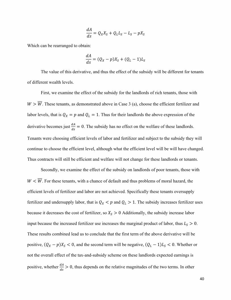
To determine the effect of a subsidy on the landlord’s expected earnings we take the derivative
of A with respect to the value of the subsidy s. This derivative is evaluated below:
40
Which can be rearranged to obtain:
1
The value of this derivative, and thus the effect of the subsidy will be different for tenants
of different wealth levels.
First, we examine the effect of the subsidy for the landlords of rich tenants, those with
. These tenants, as demonstrated above in Case 3 (a), choose the efficient fertilizer and
labor levels, that is and 1. Thus for their landlords the above expression of the
derivative becomes just 0. The subsidy has no effect on the welfare of these landlords.
Tenants were choosing efficient levels of labor and fertilizer and subject to the subsidy they will
continue to choose the efficient level, although what the efficient level will be will have changed.
Thus contracts will still be efficient and welfare will not change for these landlords or tenants.
Secondly, we examine the effect of the subsidy on landlords of poor tenants, those with
. For these tenants, with a chance of default and thus problems of moral hazard, the
efficient levels of fertilizer and labor are not achieved. Specifically these tenants oversupply
fertilizer and undersupply labor, that is and 1. The subsidy increases fertilizer uses
because it decreases the cost of fertilizer, so 0 Additionally, the subsidy increase labor
input because the increased fertilizer use increases the marginal product of labor, thus 0.
These results combined lead us to conclude that the first term of the above derivative will be
positive, 0, and the second term will be negative, 1 0. Whether or
not the overall effect of the tax-and-subsidy scheme on these landlords expected earnings is
positive, whether 0, thus depends on the relative magnitudes of the two terms. In other

41
words, whether or not the tax-and-subsidy scheme will make landlords of poor tenants better off
depends on whether the positive effect of inducing additional labor outweighs the negative effect
of inducing additional fertilizer use.
We can examine more specifically what conditions must hold for 0. We
assume 0:
1 0
Rearranging we obtain:
1
This demonstrates the result described above, for the tax-and-subsidy scheme to have a positive
effect the gain in efficiency from the induced additional labor must be greater in magnitude than
the loss in efficiency from the additional fertilizer induced.
If the above condition holds then 0 for the landlords of poor tenants. Thus,
combined with the above results I have demonstrated that if the above condition holds the tax-
and-subsidy scheme will lead to a Pareto improvement: landlords of poor tenants will be made
better off, landlords of rich tenants will have no change in expected earnings, and all tenants will
have no change in expected earnings because they will always be pushed to their reservation
income. This represents a Pareto improvement because one group is made better off and no one
is made worse off.
By demonstrating that there is a possible Pareto improvement to this equilibrium we have
demonstrated that Distribution B will not be even constrained Pareto efficient, under certain
conditions. Combined with the above result that Distribution A will be first-best Pareto efficient
(and therefore also constrained efficient), we have demonstrated that whether or not equilibrium

42
is constrained Pareto efficient can depend on the distribution of wealth. We have not
demonstrated that it will depend on the distribution in all cases of the world, just that it can under
certain conditions. In contrast, with perfect information whether or not equilibrium is Pareto
efficient would never depend on the distribution of wealth. With imperfect information this is no
longer always the case, sometimes distribution affects efficiency. Issues of equity cannot
assumed to be separated from issues of efficiency, the two can be interlinked in certain situations.
For example, in this case a more equitable distribution can lead to an equilibrium that is first-best
efficient, when a less equitable distribution leads to an equilibrium that is not even constrained
efficient.
5. Caveats and Areas for Further Research
There are two main caveats to the conclusions described above. The first applies to both
models. The second only applies to the model with fertilizer. The implications of both could be
explored further in subsequent research.
’s Dependence on
In Ray and Singh (1998) the authors acknowledge explicitly that depends on . In
other words, the conditions under which a tenant will default depend on the cropshare. This is
clear from the definition of :
, , ; :
Later in the paper, however, when Ray and Singh obtain the first-order condition for , they do
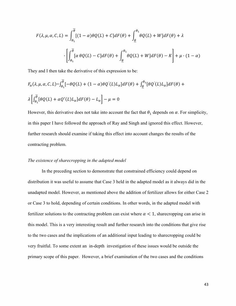
not take into account the fact that depends on . Recall, the Lagringian for the landlord’s
maximization:
43
, , , , 1
· · 1
They and I then take the derivative of this expression to be:
, , , , = 1 ′ ′
0
However, this derivative does not take into account the fact that depends on . For simplicity,
in this paper I have followed the approach of Ray and Singh and ignored this effect. However,
further research should examine if taking this effect into account changes the results of the
contracting problem.
The existence of sharecropping in the adapted model
In the preceding section to demonstrate that constrained efficiency could depend on
distribution it was useful to assume that Case 3 held in the adapted model as it always did in the
unadapted model. However, as mentioned above the addition of fertilizer allows for either Case 2
or Case 3 to hold, depending of certain conditions. In other words, in the adapted model with
fertilizer solutions to the contracting problem can exist where 1, sharecropping can arise in
this model. This is a very interesting result and further research into the conditions that give rise
to the two cases and the implications of an additional input leading to sharecropping could be
very fruitful. To some extent an in-depth investigation of these issues would be outside the
primary scope of this paper. However, a brief examination of the two cases and the conditions

44
conditions under which they would arise follows. As stated above, and demonstrated in an
appendix Case 1 will not arise in this model, just as in the unadpated model.
Case 2: participation constraint binds, share constraint does not bind
For this case we assume that the participation constraint (PC) binds and the share
constraint (SC) does not bind, that is the tenant is pushed to their reservation income and
sharecropping is present in the model. Formally, we assume 1, and 0. Unlike, the Ray
and Singh model without fertilizer we find that this case can arise under certain conditions.
Given that the participation constraint (PC) binds we have:
,
It is clear that if , (PC) would become – . Because we assume 0,
we would either have that the tenant is indebted or the above expression would be a contradiction.
Either way we can conclude that for this case to be a solution to the contracting problem .
Now we can examine the first order condition for C:
, , , 0
Which we can rearrange to:
1 0
Given that , we can conclude that 0, and thus that 1. Therefore the first
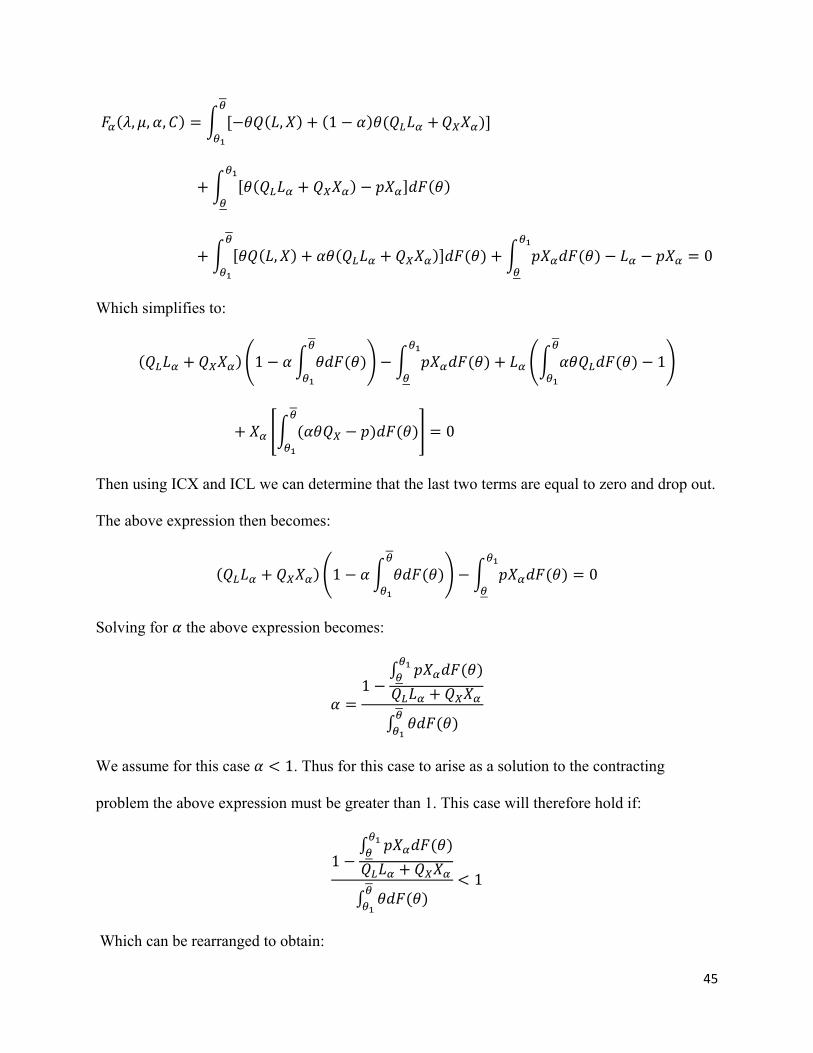
order condition for becomes:
45
, , , , 1
, 0
Which simplifies to:
1 1
0
Then using ICX and ICL we can determine that the last two terms are equal to zero and drop out.
The above expression then becomes:
1 0
Solving for the above expression becomes:
1
We assume for this case 1. Thus for this case to arise as a solution to the contracting
problem the above expression must be greater than 1. This case will therefore hold if:
11
Which can be rearranged to obtain:

46
1
Thus this case will hold as a solution to the contracting problem, and thus sharecropping
will arise, if the above expression holds. Whether or not this expression holds will depend on the
price of fertilizer and the specific form of the production function. Further examination of when
this case will arise and the intuition behind why it arises in my adapted model and not in Ray and
Singh’s model is left to later research. In short though, I surmise that the difference arise because
of the odd “double moral hazard” effect on fertilizer which is unique to my model.
Case 3: participation constraint binds, cropshare constraint binds
For this case we assume that the participation constraint (PC) binds and the cropshare
constraint (CC) binds. Formally, we assume that 0, 0, and 1. I will demonstrate
that unlike in the Ray and Singh model, where this case would always hold, this case will only
arise under certain conditions.
Following the same logic used in Case 2 we can conclude from the first-order condition
for C that 1.
Given that 1 and 1, the first-order condition for becomes:
, , , ,
,
0
Which with some cancellation and rearranging becomes:

47
1
Given that 1, ICL gives us the result that 1 0, so the second term
drops out. Similarly, given that 1, ICX can be rearranged to obtain 0,
so the last term drops out as well. Thus, we obtain:
For this case to hold we must have 0. Thus, this case will hold as a solution to the
contracting problem if the following expression holds:
0
Again whether or not this case holds depends on the price of fertilizer and specific of the
production function, as well as the distribution of . As before a more in-depth analysis of why
and when this case will hold is left to subsequent research.
Overall, we have demonstrated that with the introduction of fertilizer it is no longer clear
whether sharecropping will or will not arise in the model. This is an interesting result and would
be a viable topic for further research. Additionally, it would be interesting to study the welfare
properties of contracts when sharecropping arises and compare them to the above results for
Case 3 when sharecropping does not arise.
6. Conclusion
Stiglitz and others working in the economics of information have emphasized the many
ways that introducing imperfect information into neo-classical economic models changes the
48
basic conclusions of those models. One of those basic conclusions was that issues of equity and
efficiency could be separated: with perfect information the Pareto efficiency of equilibrium did
not depend on the initial distribution of wealth. But as Stiglitz (1987, 1985) pointed out, when
imperfect information is introduced the initial distribution of wealth can affect whether or not the
equilibrium is Pareto efficient. Thus, concerns about equity and concerns about efficiency cannot
be separated when imperfect information is taken into account; the two concerns are interrelated.
One of the reasons that distribution affects efficiency when imperfect information is
introduced is that the distribution can affect whether or not transactions that include moral hazard
will occur. For example, as Stiglitz (1991) writes, “the incentives problems associated with
sharecropping would not arise if all tenants owned the land upon which they worked.”
Sharecropping, an institution common in developing countries, is often used as an example of
moral hazard in general, as well as the way distribution can affect whether or not moral hazard
arises. Rental contracts with limited liability are another model of land tenure in developing
countries. Similar to sharecropping, land tenure contracts with limited liability lead to moral
hazard and whether or not that moral hazard will arise depends on the distribution of wealth.
Thus in this paper I have used a model of land tenure with limited liability (Ray and
Singh 2001) to demonstrate an example of the effect described by Stiglitz: that with imperfect
information whether or not the equilibrium of an economy is Pareto efficient can depend on the
distribution of wealth because the existence of moral hazard can depend on distribution. Thus, I
demonstrate examples where one distribution of wealth leads to an equilibrium that is Pareto
efficient and another distribution of wealth leads to an equilibrium that is not Pareto efficient. I
have demonstrated this effect in two slightly different ways, using two slightly different models
to do so. First, I demonstrated using the Ray and Singh (2001) model that distribution can affect
49
whether or not equilibrium was first best efficient. Then adapting their model slightly I was able
to demonstrate that under certain conditions the distribution could affect whether or not the
While this example was very specific, the conditions had to be just so to allow for one
distribution to be first-best Pareto efficient and another to be not even constrained efficient, it
demonstrated that when imperfect information is present distribution can affect efficiency in
some situations. This is not a trivial result: in models with perfect information the distribution of
wealth will never affect the Pareto efficiency of equilibrium. The separation of equity and
efficiency is one in the growing list of conclusions that could be taken for granted when perfect
information was present but that fail to hold in all cases when imperfect information is taken into
account.
Imperfect information, such as asymmetric information about labor effort between a
landlord and his tenant, is rampant in the real world. Examining, the specific ways that its
existence changes the conclusions of economic models thus seems like a worthwhile pursuit. By
demonstrating an example of one such change, described by Stiglitz but not demonstrated
formally, I hope to have added to that pursuit. Specifically, I have demonstrated that when
imperfect information is present, as it generally is in the real world, the separation of equity and
efficiency cannot be taken for granted.
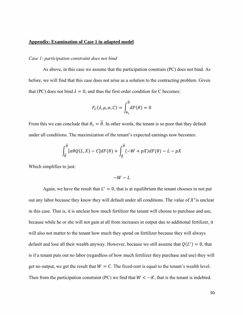
50
Appendix: Examination of Case 1 in adapted model
Case 1: participation constraint does not bind
As above, in this case we assume that the participation constrain (PC) does not bind. As
before, we will find that this case does not arise as a solution to the contracting problem. Given
that (PC) does not bind 0, and thus the first order condition for C becomes:
, , , 0
From this we can conclude that . In other words, the tenant is so poor that they default
under all conditions. The maximization of the tenant’s expected earnings now becomes:
,
Which simplifies to just:
Again, we have the result that 0, that is at equilibrium the tenant chooses to not put
out any labor because they know they will default under all conditions. The value of is unclear
in this case. That is, it is unclear how much fertilizer the tenant will choose to purchase and use,
because while he or she will not gain at all from increases in output due to additional fertilizer, it
will also not matter to the tenant how much they spend on fertilizer because they will always
default and lose all their wealth anyway. However, because we still assume that 0, that
is if a tenant puts out no labor (regardless of how much fertilizer they purchase and use) they will
get no output, we get the result that . The fixed-rent is equal to the tenant’s wealth level.
Then from the participation constraint (PC) we find that , that is the tenant is indebted.
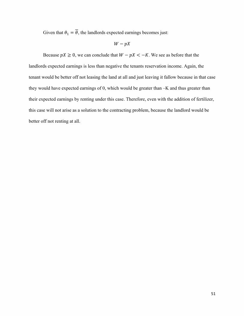
51
Given that , the landlords expected earnings becomes just:
Because 0, we can conclude that . We see as before that the
landlords expected earnings is less than negative the tenants reservation income. Again, the
tenant would be better off not leasing the land at all and just leaving it fallow because in that case
they would have expected earnings of 0, which would be greater than –K and thus greater than
their expected earnings by renting under this case. Therefore, even with the addition of fertilizer,
this case will not arise as a solution to the contracting problem, because the landlord would be
better off not renting at all.

52
References
Barhan, Pranab, Samuel Bowles and Herbert Gintis. (1999). Wealth Inequality, Wealth
Constraints and Economic Performance. Center for International and Development
Economics Research, Institute of Business and Economic Research, UC Berkeley.
Greenwald, Bruce C., and Joseph E. Stiglitz. (1986). Externalities in Economies with Imperfect
Information and Incomplete Markets. The Quarterly Journal of Economics, 101(2): 229-
264.
Hoff, Karla. (1996). Market Failures and the Distribution of Wealth: A Perspective from the
Economics of Information. Politics and Society, 24(4): 411-432.
Moral Hazard. (2006). In Collins Dictionary of Economics. Retrieved from
http://www.credoreference.com/entry/collinsecon/moral_hazard
Ray, Tridip and Nirvikar Singh. (2001). Limited liability, contractual choice, and the tenancy
ladder. Journal of Development Economics 66: 289-303.
Shapiro, Carl and Stiglitz, Joseph E. (1984). Equilibrium Unemployment as a Worker Discipline.
Device. The American Economic Review, 74(3): pp. 433-444.
Shetty, S., (1988). Limited Liability, wealth differences and tenancy contracts in agrarian
economies. Journal of Development Economics 29, 1-22.
Stiglitz, Joseph E. (1974). Incentives and Risk Sharing in Sharecropping. The Review of
Economic Studies 41(2): 219-255.
Stiglitz, Joseph E. (1985). Information and Economic Analysis: A Perspective. The Economic
Journal 95, Supplement Conference Papers, 21-41
Stiglitz, Joseph E. (1987). The Causes and Consequences of the Dependence of Quality on Price.
Journal of Economic Literature, 25(1): 1-48.

53
Stiglitz, Joseph E. (1991). The Invisible Hand and Modern Welfare Economics. NBER Working
Paper Series: Working Paper No. 3641.
Stiglitz, Joseph E. (1994). Wither Socialism? Cambridge Massachusetts: The MIT Press.
Stiglitz, Joseph E. (2000). The Contributions of the Economics of Information to Twentieth
Century Economics. The Quarterly Journal of Economics, 115(4): 1441-1478