Tree-structured multi-stage principal componentanalysis (TMPCA): theory and applications

Yuanhang Sua,∗, Ruiyuan Lina, C.-C. Jay Kuoa

aUniversity of Southern California, Ming Hsieh Department of Electrical Engineering3740 McClintock Avenue, Los Angeles, CA, United States

Abstract

A PCA based sequence-to-vector (seq2vec) dimension reduction method for

the text classification problem, called the tree-structured multi-stage principal

component analysis (TMPCA) is presented in this paper. Theoretical analysis

and applicability of TMPCA are demonstrated as an extension to our previous

work (Su, Huang, & Kuo, in press). Unlike conventional word-to-vector em-

bedding methods, the TMPCA method conducts dimension reduction at the

sequence level without labeled training data. Furthermore, it can preserve the

sequential structure of input sequences. We show that TMPCA is computa-

tionally efficient and able to facilitate sequence-based text classification tasks

by preserving strong mutual information between its input and output mathe-

matically. It is also demonstrated by experimental results that a dense (fully

connected) network trained on the TMPCA preprocessed data achieves bet-

ter performance than state-of-the-art fastText and other neural-network-based

solutions.

Keywords: dimension reduction, principal component analysis, mutual

information, text classification, embedding, neural networks

∗Corresponding AuthorPhone: +1-213-281-2388

Email addresses: suyuanhang@googlemail.com (Yuanhang Su), ruiyuanl@usc.edu(Ruiyuan Lin), cckuo@sipi.usc.edu (C.-C. Jay Kuo)

Preprint submitted to Journal of LATEX Templates October 9, 2018

arX

iv:1

807.

0822

8v2

[cs

.CL

] 7

Oct

201

8

1. Introduction

In natural language processing (NLP), dimension reduction is often required

to alleviate the so-called “curse of dimensionality” problem. This occurs when

the numericalized input data are in a sparse high-dimensional space (Bengio,

Ducharme, Vincent, & Jauvin, 2003). Such a problem partly arises from the

large size of vocabulary and partly comes from the sentence variations with simi-

lar meanings. Both contribute to high-degree data pattern diversity, and a high

dimensional space is required to represent the data in a numerical form ade-

quately. Due to the ever-increasing data in the Internet nowadays, the language

data become even more diverse. As a result, previously well-solved problems

such as text classification (TC) face new challenges (Mirnczuk & Protasiewicz,

2018; Zhang, Junbo, & LeCun, 2015). An effective dimension reduction tech-

nique remains to play a critical role in tackling these challenges. The new

dimension reduction solution should satisfy the following criteria:

• Reduce the input dimension

• Retain the input information

More specifically, dimension reduction technique should maximally preserve

the input information given the limited dimension available for representing the

input data. Different classifiers will perform differently given the same input

data. Our objective is not to find such best performing classifiers, but to propose

a dimension reduction technique that can facilitate the following classification

process.

There are many ways to reduce the language data to a compact form. The

most popular ones are the neural network (NN) based techniques (Araque,

Corcuera-Platas, Sanchez-Rada, & Iglesias, 2017; T. Chen, Xu, He, & Wang,

2017; Ghiassi, Skinner, & Zimbra, 2013; Joulin, Grave, Bojanowski, & Mikolov,

2017; Moraes, Valiati, & Neto, 2013; Zhang et al., 2015). In Bengio et al.

(2003), each element in an input sequence is first numericalized/vectorized as a

2

vocabulary-sized one-hot vector with bit “1” occupying the position correspond-

ing to the index of that word in the vocabulary. This vector is then fed into

a trainable dense network called the embedding layer. The output of the em-

bedding layer is another vector of a reduced size. In Mikolov, Sutskever, Chen,

Corrado, and Dean (2013), the embedding layer is integrated into a recurrent

NN (RNN) used for language modeling so that the trained embedding layer

can be applied to more generic language tasks. Both Bengio et al. (2003) and

Mikolov et al. (2013) conduct dimension reduction at the word level. Hence, they

are called word embedding methods. These methods are limited in modeling

“sequences of words”, which is called the sequence-to-vector (seq2vec) problem,

for two reasons. First, word embedding is trained on some particular dataset

using the stochastic gradient descent method, which could lead to overfitting

(Lai, Liu, Xu, & Zhao, 2016) easily. Second, the vector space obtained by word

embedding is still too large, it is desired to convert a sequence of words to an

even more compact form.

Among non-neural-network dimension reduction methods (K. Chen, Zhang,

Long, & Zhang, 2016; Deerwester, Dumais, Furnas, Landauer, & Harshman,

1990; Kontopoulos, Berberidis, Dergiades, & Bassiliades, 2013; Uysal, 2016;

Wei, Lu, Chang, Zhou, & Bao, 2015; Ye, Zhang, & Law, 2009), the principal

component analysis (PCA) is a popular one. In Deerwester et al. (1990), sen-

tences are first represented by vocabulary-sized vectors, where each entry holds

the frequency of a particular word in the vocabulary. Each sentence vector

forms a column in the input data matrix. Then, the PCA is used to generate a

transform matrix for dimension reduction on each sentence. Although the PCA

has some nice properties such as maximum information preservation (Linsker,

1988) between its input and output under certain constraints, we will show later

that its computational complexity is exceptionally high as the dataset size be-

comes large. Furthermore, most non-RNN-based dimension reduction methods,

such as K. Chen et al. (2016); Deerwester et al. (1990); Uysal (2016), do not

consider the positional correlation between elements in a sequence but adopt

the “bag-of-word” (BoW) representation. The sequential information is lost in

3

such a dimension reduction procedure.

To address the above-mentioned shortcomings, a novel technique, called the

tree-structured multi-stage PCA (TMPCA), was proposed in Su et al. (in press).

The TMPCA method has several interesting properties as summarized below.

1. High efficiency. Reduce the input data dimension with a small model

size at low computational complexity.

2. Low information loss. Maintain high mutual information between an

input and its dimension-reduced output.

3. Sequential preservation. Preserve the positional relationship between

input elements.

4. Unsupervised learning. Do not demand labeled training data.

5. Transparent mathematical properties. Like PCA, TMPCA is linear

and orthonormal, which makes the mathematical analysis of the system

easier.

These properties are beneficial to classification tasks that demand low-dimensional

yet highly informative data. It also relaxes the burden of data labeling in the

training stage. So TMPCA can be used as a preprocessing stage for classifica-

tion problems, a complete classification framework using TMPCA is shown in

figure below where the training TMPCA does not demand labels:

Figure 1: Integration of TMPCA to classification problems.

In this work, we present the TMPCA method and apply it to several text

classification problems such as spam email detection, sentiment analysis, news

topic identification, etc. This work is an extended version of Su et al. (in press).

As compared with Su et al. (in press), most material in Sec. 3 and Sec. 4 is

new. We present more thorough mathematical treatment in Sec. 3 by deriving

the function of the TMPCA method and analyzing its properties. Specifically,

4

the information preserving property of the TMPCA method is demonstrated

by examining the mutual information between its input and output. Also, we

provide more extensive experimental results on large text classification datasets

to substantiate our claims in Sec. 4.

The rest of this paper is organized as follows. Research on text classifica-

tion problems is reviewed in Sec. 2. The TMPCA method and its properties

are presented in Sec. 3. Experimental results are given in Sec. 4, where we

compare the performance of the TMPCA method and that of state-of-the-art

NN-based methods on text classification, including fastText (Joulin et al., 2017)

and the convolutional-neural-network (CNN) based method (Zhang et al., 2015).

Finally, concluding remarks are drawn in Sec. 5.

2. Review of Previous Work on Text Classification

Text classification has been an active research topic for two decades. Its

applications such as spam email detection, age/gender identification and senti-

ment analysis are omnipresent in our daily lives. Traditional text classification

solutions are mostly linear and based on the BoW representation. One example

is the naive Bayes (NB) method (Friedman, Dan, & Moises, 1997), where the

predicted class is the one that maximizes the posterior probability of the class

given an input text. The NB method offers reasonable performance on easy text

classification tasks, where the dataset size is small. However, when the dataset

size becomes larger, the conditional independence assumption used in likelihood

calculation required by the NB method limits its applicability to complicated

text classification tasks.

Other methods such as the support vector machine (SVM) (Joachims, 1998;

Moraes et al., 2013; Ye et al., 2009) fit the decision boundary in a hand-crafted

feature space of input texts. Finding representative features of input texts is

actually a dimension reduction problem. Commonly used features include the

frequency that a word occurs in a document, the inverse-document-frequency

(IDF), the information gain (K. Chen et al., 2016; Salton & Buckley, 1988; Uysal,

5

2016; Yang & Pedersen, 1997), etc. Most SVM models exploit BoW features,

and they do not consider the position information of words in sentences.

The word position in a sequence can be better handled by the CNN solu-

tions since they process the input data in sequential order. One example is the

character level CNN (char-CNN) as proposed in Zhang et al. (2015). It repre-

sents an input character sequence as a two-dimensional data matrix with the

sequence of characters along one dimension and the one-hot embedded char-

acters along the other one. Any character exceeding the maximum allowable

sequence length is truncated. The char-CNN has 6 convolutional (conv) lay-

ers and 3 fully-connected (dense) layers. In the conv layer, one dimensional

convolution is carried out on each entry of the embedding vector.

RNNs offer another NN-based solution for text classification (T. Chen et

al., 2017; Mirnczuk & Protasiewicz, 2018). An RNN generates a compact yet

rich representation of the input sequence and stores it in form of hidden states

of the memory cell. It is the basic computing unit in an RNN. There are

two popular cell designs: the long short-term memory (LSTM) (Hochreiter &

Schmidhuber, 1997) and the gate recurrent unit (GRU) (Cho et al., 2014). Each

cell takes each element from a sequence sequentially as its input, computes an

intermediate value, and updates it dynamically. Such a value is called the

constant error carousal (CEC) in the LSTM and simply a hidden state in the

GRU. Multiple cells are connected to form a complete RNN. The intermediate

value from each cell forms a vector called the hidden state. It was observed in

Elman (1990) that, if a hidden state is properly trained, it can represent the

desired text patterns compactly, and similar semantic word level features can

be grouped into clusters. This property was further analyzed in Su, Huang, and

Kuo (Unpublished). Generally speaking, for a well designed representational

vector (i.e. the hidden state), the computing unit (or the memory cell) can

exploit the word-level dependency to facilitate the final classification task.

Another NN-based model is the fastText (Joulin et al., 2017). As shown

in Fig. 2, it is a multi-layer perceptron composed by a trainable embedding

layer, a hidden mean layer and a softmax dense layer. The hidden vector is

6

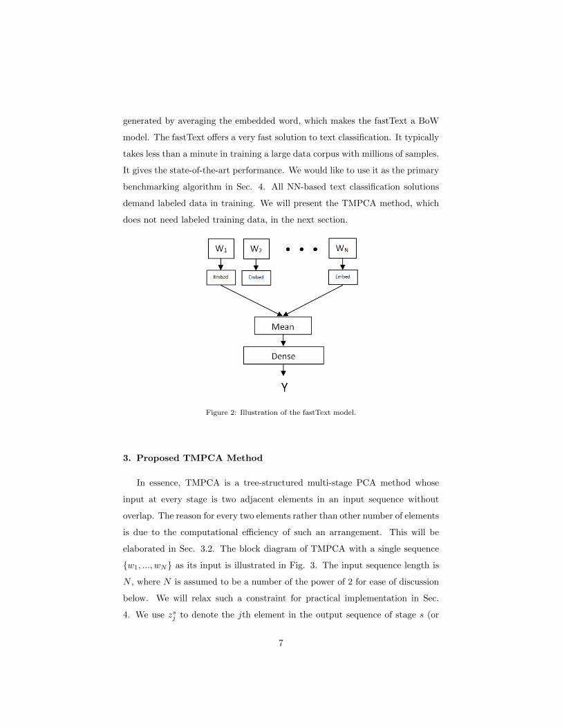
generated by averaging the embedded word, which makes the fastText a BoW

model. The fastText offers a very fast solution to text classification. It typically

takes less than a minute in training a large data corpus with millions of samples.

It gives the state-of-the-art performance. We would like to use it as the primary

benchmarking algorithm in Sec. 4. All NN-based text classification solutions

demand labeled data in training. We will present the TMPCA method, which

does not need labeled training data, in the next section.

Figure 2: Illustration of the fastText model.

3. Proposed TMPCA Method

In essence, TMPCA is a tree-structured multi-stage PCA method whose

input at every stage is two adjacent elements in an input sequence without

overlap. The reason for every two elements rather than other number of elements

is due to the computational efficiency of such an arrangement. This will be

elaborated in Sec. 3.2. The block diagram of TMPCA with a single sequence

{w1, ..., wN} as its input is illustrated in Fig. 3. The input sequence length is

N , where N is assumed to be a number of the power of 2 for ease of discussion

below. We will relax such a constraint for practical implementation in Sec.

4. We use zsj to denote the jth element in the output sequence of stage s (or

7

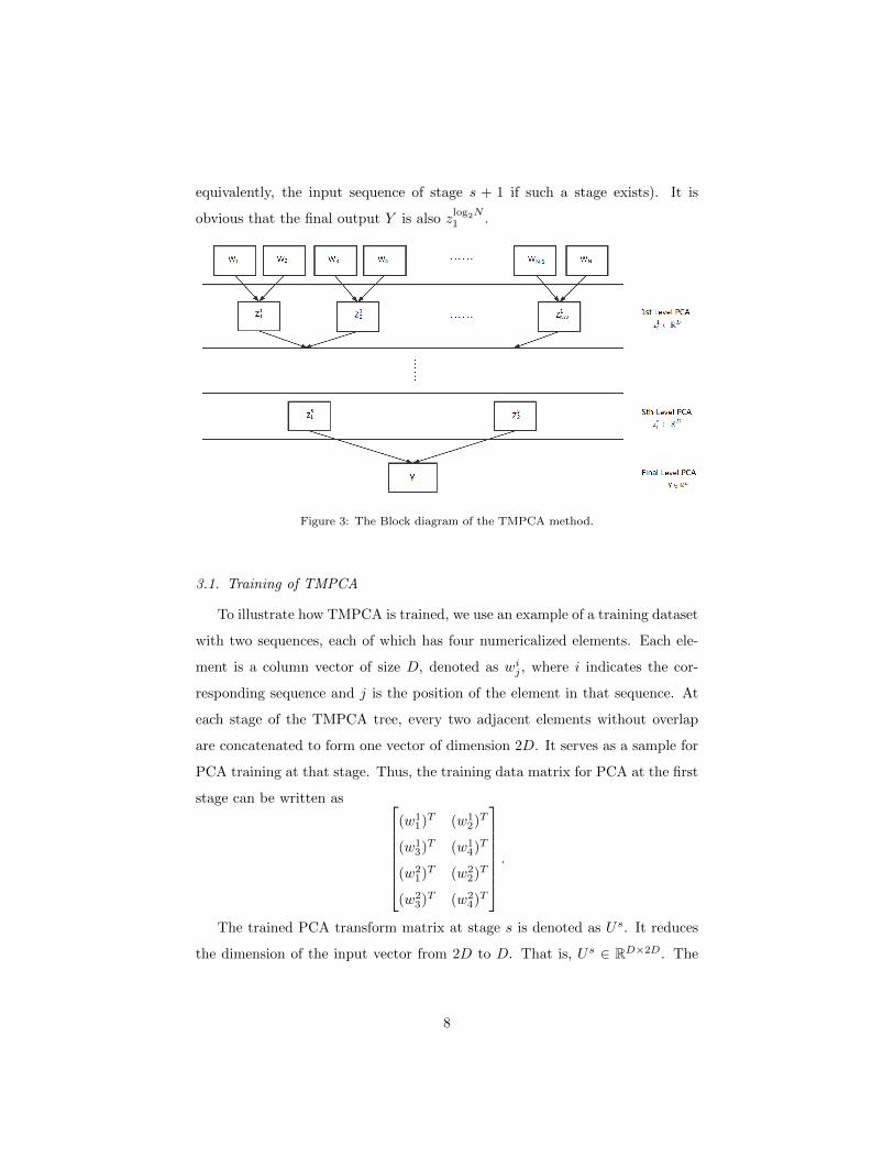
equivalently, the input sequence of stage s + 1 if such a stage exists). It is

obvious that the final output Y is also zlog2N1 .

Figure 3: The Block diagram of the TMPCA method.

3.1. Training of TMPCA

To illustrate how TMPCA is trained, we use an example of a training dataset

with two sequences, each of which has four numericalized elements. Each ele-

ment is a column vector of size D, denoted as wij , where i indicates the cor-

responding sequence and j is the position of the element in that sequence. At

each stage of the TMPCA tree, every two adjacent elements without overlap

are concatenated to form one vector of dimension 2D. It serves as a sample for

PCA training at that stage. Thus, the training data matrix for PCA at the first

stage can be written as (w1

1)T (w12)T

(w13)T (w1

4)T

(w21)T (w2

2)T

(w23)T (w2

4)T

.

The trained PCA transform matrix at stage s is denoted as Us. It reduces

the dimension of the input vector from 2D to D. That is, Us ∈ RD×2D. The

8

training matrix at the first stage is then transformed by U1 to(z11)T

(z12)T

(z13)T

(z14)

, z11 = U1(

w11

w12

), z12 = U1(

w13

w14

), z13 = U1(

w21

w22

), z14 = U1(

w23

w24

),

After that, we rearrange the elements on the transformed training matrix to

form (z11)T (z12)T

(z13)T (z14)T

.It serves as the training matrix for the PCA at the second stage. We repeat

the training data matrix formation, the PCA kernel determination and the PCA

transform steps recursively at each stage until the length of the training samples

becomes 1. It is apparent that, after one-stage TMPCA, the sample length is

halved while the element vector size keeps the same as D. The dimension

evolution from the initial input data to the ultimate transformed data is shown

in Table 1. Once the TMPCA is trained, we can use it to transform test data

by following the same steps except that we do not need to compute the PCA

transform kernels at each stage.

Table 1: Dimension evolution from the input to the output in the TMPCA method.

Sequence length Element vector size

Input sequence N D

Output sequence 1 D

3.2. Computational Complexity

We analyze the time complexity of TMPCA training in this section. Consider

a training dataset of M samples, where each sample is of length N with element

vectors of dimension D. To determine the PCA model for this training matrix of

dimension RM×ND, it requires O(MN2D2) to compute the covariance matrix,

9

and O(N3D3) to compute the eigenvalues of the covariance matrix. Thus, the

complexity of PCA can be written as

O(fPCA) = O(N3D3 +MN2D2

). (1)

The above equation can be simplified by comparing the value of M with ND.

We do not pursue along this direction furthermore since it is problem dependent.

Suppose that we concatenate non-overlapping P adjacent elements at each

stage of TMPCA. The dimension of the training matrix at stage s is M NP s ×PD.

Then, the total computational complexity of TMPCA can be written as

O(fTMPCA) = O( logP N∑

s=1

((PD)3 +M

N

P s(PD)2

)),

= O(

(P 3logPN)D3 +MP 2

P − 1(N − 1)D2

). (2)

The complexity of TMPCA is an increasing function in P . This can be

verified by non-negativity of its derivative with respect to P . Thus, the worst

case is P = N , which is simply the traditional PCA applied to the entire samples

in a single stage. When P = 2, the TMPCA achieves its optimal efficiency. Its

complexity is

O(fTMPCA) = O(

8(log2N)D3 + 4M(N − 1)D2),

= O(

2(log2N)D3 +M(N − 1)D2). (3)

By comparing Eqs. (3) and (1), we see that the time complexity of the tradi-

tional PCA grows at least quadratically with sentence length N (since P = N)

while that of TMPCA grows at most linearly with N .

3.3. System Function

To analyze the properties of TMPCA, we derive its system function in closed

form in this section. In particular, we will show that, similar to PCA, TMPCA is

a linear transform and its transformation matrix has orthonormal rows. For the

rest of this paper, we assume that the length of the input sequence is N N = 2L,

10

where L is the total stage number of TMPCA. The input is mean-removed so

that its mean is 0.

We denote the element of the input sequence by wj , where wj ∈ RD and

j ∈ {1, ..., N}. Then, the input sequence X to TMPCA is a column vector in

form of

XT = [wT1 , · · · , wT

N ]. (4)

We decompose PCA transform matrices, Us, at stage s into two equal-sized

block matrices as

Us = [Us1 , U

s2 ], (5)

where Usj ∈ RD×D, and where j ∈ {1, 2}. The output of TMPCA is Y ∈ RD

With notations inherited from Sections 3.1 and 3.2, we can derive the closed-

form expression of TMPCA by induction (see Appendix A). That is, we have

Y = UX, (6)

U = [U1, ..., UN ], (7)

Uj =

L∏s=1

Usfj,s ,∀j ∈ {1, ..., N} (8)

fj,s = bL(j − 1)s + 1,∀j, s. (9)

where bL(x)s is the sth digit of L-binarized form of x. TMPCA is a linear

transform as shown in Eq. 6. Also, since there always exist real valued eigen-

vectors to form the PCA transform matrix, U , Uj and {Usj }2j=1 are all real

valued matrices.

To show that U has orthonormal rows, we first examine the properties of

matrix K = [U1, U2]. By setting

A =

L∏s=2

Usf1,s =

L∏s=2

Usf2,s ,

we obtain K = [AU11 , AU

12 ]. Since matrix [U1

1 , U12 ] is a PCA transform matrix,

it has orthonormal rows. Denote < · >ij as the inner product between the ith

row and jth row of matrix ·, we conclude that the < K >ij=< A >ij using the

following property.

11

Lemma 1. Given K = [AB1, AB2], where [B1, B2] has orthonormal rows, then

< K >ij=< A >ij.

We then let

Ksm = [As

mUs1 , A

smU

s2 ], (10)

where s ∈ {1, ..., L} indicates the stage, and m ∈ {1, ..., N2s }, and

Asm =

L∏k=s+1

Ukfm,k−s

, and AL1 = I, (11)

where I is the identity matrix. At stage 1, K1m = [U2m−1, U2m], so U =

[K11 , ...,K

1N/2]. Since < U >ij=

∑N/2m=1 < K1

m >ij , according to 1, Eqs. (10)-

(11) we have

< U >ij =

N/2∑m=1

< A1m >ij ,

=

N/4∑m=1

< K2m >ij=

N/4∑m=1

< A2m >ij ,

. . .

=< KL1 >ij=< [UL

1 , UL2 ] >ij , (12)

Thus, U has orthonormal rows.

3.4. Information Preservation Property

Besides its low computation complexity, linearity and orthonormality, TM-

PCA can preserve the information of its input effectively so as to facilitate the

following classification process. To show this point, we investigate the mutual

information (Bennasar, Hicks, & Setchi, 2015; Linsker, 1988) between the input

and the output of TMPCA.

Here, the input to the TMPCA system is modeled as

X = G+ n, (13)

where G and n are used to model the ground truth semantic signal and the noise

component in the input, respectively. In other words, G carries the essential

12

information for the text classification task while n is irrelevant to (or weakly cor-

related) the task. We are interested in finding the mutual information between

output Y and ground truth G.

By following the framework in Linsker (1988), we make the following as-

sumptions:

1. Y ∼ N(y,V );

2. n ∼ N(0,B), where B = σ2I;

3. n is uncorrelated with G.

In above, N denotes the multivariant Gaussian density function. Then, the

mutual information between Y and G can be computed as

I(Y,G) =EY,G

(lnP (Y |G)

P (Y )

),

=EY,G

(lnN(Ug,UBUT )

N(y,V )

),

=1

2ln

|V ||UBUT |

− 1

2EY,G

[(y − Ug)T (UBUT )−1(y − Ug)

]+

1

2EY,G

[(y − y)TV −1(y − y)

], (14)

where y ∈ Y , g ∈ G, and P (·), | · | and EX denote the probability density func-

tion, the determinant and the expectation of random variable X, respectively.

It is straightforward to prove the following lemma,

Lemma 2. For any random vector X ∈ RD with covariance matrix Kx, the

following equality holds

EX{(x− x)T (Kx)−1(x− x)} = D.

Then, based on this lemma, we can derive that

I(Y,G) =1

2ln|V |σ2D

. (15)

The above equation can be interpreted below. Given input signal noise σ,

the mutual information can be maximized by maximizing the determinant of

the output covariance matrix. Since TMPCA maximizes the covariance of its

13

output at each stage, TMPCA will deliver an output with the largest mutual

information at the corresponding stage. We will show experimentally in Section

4 that the mutual information of TMPCA is significantly larger than that of

the mean operation and close to that of PCA.

4. Experiments

4.1. Datasets

We tested the performance of the TMPCA method on twelve datasets of

various text classification tasks as shown in Table 2. Four of them are smaller

datasets with at most 10,000 training samples. The other eight are large-scale

datasets (Zhang et al., 2015) with training samples ranging from 120 thousands

to 3.6 millions.

Table 2: Selected text classification datasets.

# of Class Train Samples Test Samples # of Tokens

spam 2 5,574 558 14,657

sst 2 8409 1803 18,519

semeval 2 5098 2034 25,167

imdb 2 10162 500 20,892

agnews 4 120,000 7,600 188,111

sogou 5 450,000 60,000 800,057

dbpedia 14 560,000 70,000 1,215,996

yelpp 2 560,000 38,000 1,446,643

yelpf 5 650,000 50,000 1,622,077

yahoo 10 1,400,000 60,000 4,702,763

amzp 2 3,600,000 400,000 4,955,322

amzf 5 3,000,000 650,000 4,379,154

These datasets are briefly introduced below.

14

1. SMS Spam (spam) (Almeida, Hidalgo, & Yamakami, 2011). It is a

dataset collected for mobile Spam email detection. It has two target

classes: “Spam” and “Ham”.

2. Stanford Sentiment Treebank (sst) (Socher et al., 2013). It is a

dataset for sentiment analysis. The labels are generated using the Stanford

CoreNLP toolkit (Stanford, 2018). The sentences labeled as very negative

or negative are grouped into one negative class. Sentences labeled as very

positive or positive are grouped into one positive class. We keep only

positive and negative sentences for training and testing.

3. Semantic evaluation 2013 (semeval) (Wilson et al., 2013). It is a

dataset for sentiment analysis. We focus on Sentiment task-A with pos-

itive/negative two target classes. Sentences labeled as “neutral” are re-

moved.

4. Cornell Movie review (imdb) (Bo & Lee, 2005). It is a dataset for

sentiment analysis for movie reviews. It contains a collection of movie

review documents with their sentiment polarity (i.e., positive or negative).

5. AG’s news (agnews) (Zhang & Zhao, 2005). It is a dataset for news

categorization. Each sample contains the news title and description. We

combine the title and description into one sentence by inserting a colon in

between.

6. Sougou news (sogou) (Zhang & Zhao, 2005). It is a Chinese news

categorization dataset. Its corpus uses a phonetic romanization of Chinese.

7. DBPedia (dbpedia) (Zhang & Zhao, 2005). It is an ontology categoriza-

tion dataset with its samples extracted from the Wikipedia. Each training

sample is a combination of its title and abstract.

8. Yelp reviews (yelpp and yelpf) (Zhang & Zhao, 2005). They are

sentiment analysis datasets. The Yelp review full (yelpf) has target classes

ranging from one to five stars. The one star is the worst while five stars

the best. The Yelp review polarity (yelpp) has positive/negative polarity

labels by treating stars 1 and 2 as negative, stars 4 and 5 positive and

omitting star 3 in the polarity dataset.

15

9. Yahoo! answers (yahoo) (Zhang & Zhao, 2005). It is a topic classifi-

cation dataset for Yahoo’s question and answering corpus.

10. Amazon reviews (amzp and amzf) (Zhang & Zhao, 2005). These two

datasets are similar to Yelp reviews but of much larger sizes. They are

about Amazon product reviews.

4.2. Experimental Setup

We compare the performance of the following three methods on the four

small datasets:

1. TMPCA-preprocessed data followed by the dense network (TMPCA+Dense);

2. fastText;

3. PCA-preprocessed data followed by the dense network (PCA+Dense).

For the eight larger datasets, we compare the performance of six methods.

They are:

1. TMPCA-preprocessed data followed by the dense network (TMPCA+Dense);

2. fastText;

3. PCA-preprocessed data followed by the dense network (PCA+Dense);

4. char-CNN (Zhang et al., 2015);

5. LSTM (an RNN based method) (Zhang et al., 2015);

6. BoW (Zhang et al., 2015).

Besides training time, classification accuracy and F1 macro score, we com-

pute the mutual information between the input and the output of the TMPCA

method, the mean operation (used by fastText for hidden vector computation)

and the PCA method, respectively. Note that the mean operation can be ex-

pressed as a linear transform in form of

Y =1

N[I, ..., I]X, (16)

where I ∈ RD×D is the identity matrix and the mean transform matrix has N

I’s. The mutual information between the input and the output of the mean

16

operation can be calculated as

I(Y,G) =1

2ln|V |ND

σ2D. (17)

For fixed noise variance σ2, we can compare the mutual information of the

input and the output of different operations by comparing their associated |V |,

|V |ND.

To illustrate the information preservation property of TMPCA across multi-

ple stages, we compute the output energy, which is the sum of squared elements

in a vector/tensor, as a percentage of its input energy, and see how the en-

ergy values decrease as the stage number becomes bigger. Such investigation

is meaningful since the energy indicates signal’s variance in a TMPCA system.

The variance is a good indicator of information richness. The energy percentage

is an indicator of the amount of input information that is preserved after one

TMPCA stage. We compute the total energy of multiple sentences by adding

them together.

To numericalize the input data, we first remove the stop words from sentences

according to the stop-word list, tokenize sentences and, then, stem tokens using

the python natural language toolkit (NLTK). Afterwards, we use the fastText-

trained embedding layer to embed the tokens into vectors of size 10. The tokens

are then concatenated to form a single long vector.

In TMPCA, to ensure that the input sequence is of the same length and

equal to a power of 2, we assign a fixed input length, N = 2L, to all sentences of

length N ′. If N ′ < N , we preprocess the input sequence by padding it to be of

length N with a special symbol. If N ′ > N , we shorten the input sequence by

dividing it into N segments and calculating the mean of numericalized elements

in each segment. The new sequence is then formed by the calculated means. The

reason of dividing a sequence into segments is to ensure consecutive elements as

close as possible. Then, the segmentation of an input sequence can be conducted

as follows.

1. Calculate the least number of elements that each segment should have:

d = floor(N ′/N), where floor denotes flooring operation.

17

2. Then we allocate the remaining r = N ′ − dN elements by adding one

more element to every other floor(N/r) segments until there are no more

elements left.

To give an example, to partition the sequence {w1, · · · , w10} into four segments,

we have 3, 2, 3, 2 elements in these four segments, respectively. That is, they

are: {w1, w2, w3}, {w4, w5}, {w6, w7, w8}, {w9, w10}.

For large-scale datasets, we calculate the training data covariance matrix

for TMPCA incrementally by calculating the covariance matrix on each smaller

non-overlapping chunk of the data and, then, adding the calculated matrices

together. The parameters used in dense network training are shown in Table 3.

For TMPCA and PCA, the numericalized input data are first preprocessed to a

fixed length and, then, have their means removed. TMPCA, fastText and PCA

were trained on Intel Core i7-5930K CPU. The dense network was trained on

the GeForce GTX TITAN X GPU. TMPCA and PCA were not optimized for

multi-threading whereas fastText was run on 12 threads in parallel.

Table 3: Parameters in dense network training.

Input size 10

Output size # of target class

Training steps 5 epochs

Learning rate 0.5

Training optimizer Adam (Kingma & Ba, 2015)

4.3. Results

4.3.1. Performance Benchmarking with State-of-the-Art Methods

We report the results of using the TMPCA method for feature extraction

and the dense network for decision making in terms of test accuracy, F1 macro

score, training time and number of model parameters for text classification

with respect to the eight large datasets. Furthermore, we conduct performance

18

benchmarking between the proposed TMPCA model against several state-of-

the-art models.

The bigram training data for the dense network are generated by concatenat-

ing the bigram representation of the samples to their original. For example, for

sample of {w1, w2, w3}, after the bigram process, it becomes {w1, w2, w3, w1w2, w2w3}.

The accuracy and training time for models other than TMPCA are from their

original reports in Zhang et al. (2015) and Joulin et al. (2017). There are two

char-CNN models. We report the test accuracy of the better model in Table 4

and the time and model complexity of the smaller model in Tables 5 and 6. The

time reported for char-CNN and fastText in Table 5 is for one epoch only. We

only report the F1 macro score of TMPCA+Dense against the fastText since

firstly fastText has the best performance among the other models and secondly

it takes very long time to generate the results for other models (see Table 5)

It is obvious that the TMPCA+Dense method is much faster. Besides, it

achieves better or commensurate performance as compared with other state-

of-the-art methods. In addition, the number of parameters of TMPCA is also

much less than other models as shown in Table 6.

Table 4: Performance comparison (accuracy (%)/F1 macro) of different TC models.

BoW LSTM char-CNN fastTextTMPCA+Dense

(bigram, N = 8)

agnews 88.8 86.1 87.2 91.5/0.921 92.1/0.930

sogou 92.9 95.2 95.1 93.9/0.970 97.0/0.982

dbpedia 96.6 98.6 98.3 98.1/0.986 98.6/0.981

yelpp 92.2 94.7 94.7 93.8/0.950 95.1/0.958

yelpf 58.0 58.2 62.0 60.4/0.578 64.1/0.594

yahoo 68.9 70.8 71.2 72.0/0.695 72.0/0.688

amzp 90.4 93.9 94.5 91.2/0.934 94.2/0.962

amzf 54.6 59.4 59.5 55.8/0.533 59.0/0.587

19

Table 5: Comparison of training time for different models.

small char-CNN/epoch fastText/epochTMPCA+Dense

(bigram, N = 8)

agnews 1h 1s 0.025s

sogou - 7s 0.081s

dbpedia 2h 2s 0.101s

yelpp - 3s 0.106s

yelpf - 4s 0.116s

yahoo 8h 5s 0.229s

amzp 2d 10s 0.633s

amzf 2d 9s 0.481s

Table 6: Comparison of model parameter numbers in different models.

small char-CNN/epoch fastText/epochTMPCA+Dense

(bigram, N = 8)

agnews

2.7e+06

1.9e+06

600

sogou 8e+06

dbpedia 1.2e+07

yelpp 1.4e+07

yelpf 1.6e+07

yahoo 4.7e+07

amzp 5e+07

amzf 4.4e+07

20

4.3.2. Comparison between TMPCA and PCA

We compare the performance between TMPCA+Dense and PCA+Dense to

shed light on the property of TMPCA. Their input are unigram data in each

original dataset. We compare their training time in Table 7. It clearly shows

the advantage of TMPCA in terms of computational efficiency. TMPCA takes

less than one second for training in most datasets. As the length of the input

sequence is longer, the training time of TMPCA grows linearly. In contrast, it

grows much faster in the PCA case.

To show the information preservation property of TMPCA, we include fast-

Text in the comparison. Since the difference between these three models is the

way to compute the hidden vector, we compare TMPCA, mean operation (used

by fastText), and PCA. We show the accuracy for input sequences of length 2, 4,

8, 16 ad 32 in Fig. 4. They correspond to the 1-, 2-, 3-, 4- and 5-stage TMPCA,

respectively. We show two relative mutual information values in Table 8 and

Table 9. Table 8 provides the mutual information ratio between TMPCA and

mean. Table 9 offers the mutual information ratio between PCA and TMPCA.

We see that TMPCA is much more capable than mean and is comparable with

PCA in preserving the mutual information. Although higher mutual informa-

tion does not always translate into better classification performance, there is

a strong correlation between them. This substantiates our mutual information

discussion. We should point out that the mutual information on different in-

puts (in our case, different N values) is not directly comparable. Thus, a higher

relative mutual information value on longer inputs cannot be interpreted as con-

taining richer information and, consequently, higher accuracy. We observe that

the dense network achieves its best performance when N = 4 or 8.

To understand information loss at each TMPCA, we plot their energy per-

centages in Fig. 5 where the input has a length of N = 32. For TMPCA,

the energy drops as the number of stage increases, and the sharp drop usually

happens after 2 or 3 stages. This observation is confirmed by the results in

Fig. 4. For performance benchmarking, we provide the energy percentage of

21

PCA in the same figure. Since the PCA has only one stage, we use a horizontal

line to represent the percentage level. Its value is equal or slightly higher than

the energy percentage at the final stage of TMPCA. This is collaborated by

the closeness of their mutual information values in Table 9. The information

preserving and the low computational complexity properties make TMPCA an

excellent dimension reduction pre-processing tool for text classification.

Table 7: Comparison of training time in seconds (TMPCA/PCA).

N = 4 N = 8 N = 16 N = 32

spam 0.007/0.023 0.006/0.090 0.007/0.525 0.011/7.389

sst 0.007/0.023 0.006/0.090 0.008/0.900 0.009/5.751

semeval 0.005/0.017 0.007/0.111 0.021/2.564 0.009/5.751

imdb 0.006/0.019 0.008/0.114 0.009/0.781 0.009/6.562

agnews 0.014/0.053 0.017/0.325 0.033/4.100 0.061/47.538

sogou 0.029/0.111 0.053/1.093 0.134/17.028 0.214/173.687

dbpedia 0.039/0.145 0.092/1.886 0.125/15.505 0.348/279.405

yelpp 0.037/0.145 0.072/1.517 0.163/20.740 0.272/222.011

yelpf 0.035/0.137 0.072/1.517 0.157/19.849 0.328/268.698

yahoo 0.068/0.269 0.129/2.714 0.322/40.845 0.787/642.278

amzp 0.184/0.723 0.379/8.009 0.880/112.021 1.842/1504.912

amzf 0.167/0.665 0.351/7.469 0.778/99.337 1.513/1237.017

5. Conclusion

An efficient language data dimension reduction technique, called the TM-

PCA method, was proposed for TC problems in this work. TMPCA is a multi-

stage PCA in special form, and it can be described by a transform matrix

with orthonormal rows. It can retain the input information by maximizing the

mutual information between its input and output, which is beneficial to TC

problems. It was shown by experimental results that a dense network trained

22

2 4 8 16 320.97

0.98

0.99

1spam

(a)

2 4 8 16 320.75

0.8

0.85

0.9sst

(b)

2 4 8 16 320.77

0.78

0.79

0.8semeval

(c)

2 4 8 16 320.72

0.74

0.76imdb

(d)

2 4 8 16 320.9

0.91

0.92agnews

(e)

2 4 8 16 320.93

0.94

0.95sogou

(f)

2 4 8 16 320.9

0.95

1dbpedia

(g)

2 4 8 16 320.935

0.94

0.945

0.95yelpp

(h)

2 4 8 16 320.58

0.59

0.6yelpf

(i)

2 4 8 16 320.7

0.71

0.72yahoo

(j)

2 4 8 16 320.91

0.915

0.92amzp

(k)

2 4 8 16 320.52

0.54

0.56

0.58amzf

(l)

Figure 4: Comparison of testing accuracy (%) of fastText (dotted blue), TMPCA+Dense (red

solid), and PCA+Dense (green head dotted), where the horizontal axis is the input length N .

23

Table 8: The relative mutual information ratio (TMPCA versus Mean).

N = 2 N = 4 N = 8 N = 16 N = 32

spam 1.32e+02 7.48e+05 2.60e+12 5.05e+14 9.93e+12

sst 8.48e+03 1.22e+10 1.28e+15 8.89e+15 9.17e+13

semeval 5.52e+03 1.13e+09 3.30e+14 4.78e+15 1.67e+13

imdb 1.34e+04 3.49e+09 1.89e+14 8.73e+14 1.05e+13

agnews 4.10e+05 5.30e+10 7.09e+11 3.56e+12 6.11e+12

sogou 5.53e+08 1.37e+13 6.74e+13 5.40e+13 4.21e+13

dbpedia 20.2 111 227 814 306

yelpp 8.42e+04 2.79e+11 3.85e+15 5.65e+16 1.46e+16

yelpf 2.29e+07 1.90e+11 5.92e+12 5.42e+12 1.58e+12

yahoo 6.7 9.1 9.9 5.8 1.5

amzp 7.34e+05 4.48e+11 1.24e+16 1.15e+18 2.75e+18

amzf 3.09e+06 1.47e+10 3.38e+11 1.48e+12 2.37e+12

Table 9: The relative mutual information ratio (PCA versus TMPCA).

N = 4 N = 8 N = 16 N = 32

spam 1.04 1.00 1.00 1.49

sst 1.00 1.00 1.00 1.36

semeval 0.99 1.00 1.00 1.09

imdb 1.02 1.00 1.00 1.29

agnews 1.00 1.01 1.40 2.92

sogou 1.00 1.20 1.66 5.17

dbpedia 1.16 1.63 1.65 1.75

yelpp 1.00 1.00 1.00 1.13

yelpf 1.00 1.01 1.01 1.10

yahoo 1.01 1.30 1.94 8.78

amzp 1.00 1.00 1.00 1.10

amzf 1.00 1.00 1.03 1.41

24

1 2 3 4 540

60

80

100spam

(a)

1 2 3 4 50

50

100sst

(b)

1 2 3 4 50

50

100semeval

(c)

1 2 3 4 50

50

100imdb

(d)

1 2 3 4 50

50

100agnews

(e)

1 2 3 4 50

50

100sogou

(f)

1 2 3 4 50

50

100dbpedia

(g)

1 2 3 4 50

50

100yelpp

(h)

1 2 3 4 50

50

100yelpf

(i)

1 2 3 4 50

50

100yahoo

(j)

1 2 3 4 540

60

80

100amzp

(k)

1 2 3 4 50

50

100amzf

(l)

Figure 5: The energy of TMPCA (red solid) and PCA (green head dotted) coefficients is

expressed as percentages of the energy of input sequences of length N = 32, where the

horizontal axis indicates the TMPCA stage number while PCA has only one stage.

25

on the TMPCA preprocessed data outperforms state-of-the-art fastText, char-

CNN and LSTM in quite a few TC datasets. Furthermore, the number of

parameters used by TMPCA is an order of magnitude smaller than other NN-

based models. Typically, TMPCA takes less than one second training time on

a large-scale dataset that has millions of samples. To conclude, TMPCA is a

powerful dimension reduction pre-processing tool for text classification for its

low computational complexity, low storage requirement for model parameters

and high information preserving capability.

6. Declarations of interest

Declarations of interest: none

7. Acknowledgements

This research did not receive any specific grant from funding agencies in the

public, commercial, or not-for-profit sectors.

Appendix A: Detailed Derivation of TMPCA System Function

We use the same notations in Sec. 3. For stage s > 1, we have:

zsj = Us

zs−12j−1

zs−12j

= Us1z

s−12j−1 + Us

2zs−12j , (18)

where j = 1, · · · , N2s . When s = 1, we have

z1j = U11w2j−1 + U1

2w2j (19)

From Eqs. (18) and (19), we get

Y = zL1 =

N∑j=1

( L∏s=1

Usfj,s

)wj , (20)

fj,s = bL(j − 1)s + 1, (21)

26

where bL(x)s is the sth digit of the binarization of x of length L. Eq. (20) can

be further simplified to Eq. (6). For example, if N = 8, we obtain

Y =U31U

21U

11w1 + U3

1U21U

12w2 + U3

1U22U

11w3 + U3

1U22U

12w4+

U32U

21U

11w5 + U3

2U21U

12w6 + U3

2U22U

11w7 + U3

2U22U

12w8. (22)

The superscripts of Usj are arranged in the stage order of L,L − 1, ..., 1. The

subscripts are shown in Table 10. This is the reason that binarization is required

to express the subscripts in Eqs. (6) and (20).

Table 10: Subscripts of Usj

w1 w2 w3 w4 w5 w6 w7 w8

1,1,1 1,1,2 1,2,1 1,2,2 2,1,1 2,1,2 2,2,1 2,2,2

References

[dataset] Almeida, T. A., Hidalgo, J. M. G., & Yamakami, J. M. (2011). Con-

tributions to the study of sms spam filtering: New collection and results.

https://archive.ics.uci.edu/ml/datasets/sms+spam+collection.

Araque, O., Corcuera-Platas, I., Sanchez-Rada, J. F., & Iglesias, C. A. (2017,

Jul). Enhancing deep learning sentiment analysis with ensemble tech-

niques in social applications. Expert Systems with Applications, 77 , 236–

246.

Bengio, Y., Ducharme, R., Vincent, P., & Jauvin, C. (2003, Feb). A neu-

ral probabilistic language model. Journal of Machine Learning Research,

3 (2), 1137–1155.

Bennasar, M., Hicks, Y., & Setchi, R. (2015). Feature selection using joint mu-

tual information maximisation. Expert Systems with Applications, 42 (22),

8520–8532.

[dataset] Bo, P., & Lee, L. (2005). sentence polarity dataset. http://www.cs

.cornell.edu/people/pabo/movie-review-data/.

27

Chen, K., Zhang, Z., Long, J., & Zhang, H. (2016, Dec). Turning from tf-idf

to tf-igm for term weighting in text classification. Expert Systems with

Applications, 66 , 245–260.

Chen, T., Xu, R., He, Y., & Wang, X. (2017, Apr). Improving sentiment

analysis via sentence type classification using bilstm-crf and cnn. Expert

Systems with Applications, 72 , 221–230.

Cho, K., Merrienboer, B. v., Gulcehre, C., Bahdanau, D., Bougares, F.,

Schwenk, H., & Bengio, Y. (2014). Learning phrase representations using

rnn encoder-decoder for statistical machine translation. In Proceedings of

the 2014 conference on empirical methods in natural language processing

(pp. 1724–1734). Doha, Qatar: Association for Computational Linguis-

tics.

Deerwester, S., Dumais, T. S., Furnas, W. G., Landauer, K. T., & Harshman,

R. (1990). Indexing by latent semantic analysis. Journal of the American

society for information science, 41 (6), 391–407.

Elman, J. (1990). Finding structure in time. Cognitive Science, 14 (2), 179-211.

Friedman, N., Dan, G., & Moises, G. (1997). Bayesian network classifiers.

Machine learning , 29 (2-3), 131–163.

Ghiassi, M., Skinner, J., & Zimbra, D. (2013). Twitter brand sentiment analy-

sis: A hybrid system using n-gram analysis and dynamic artificial neural

network. Expert Systems with Applications, 40 (16), 6266–6282.

Hochreiter, S., & Schmidhuber, J. (1997). Long short-term memory. Neural

Computation, 9 (8), 1735–1780.

Joachims, T. (1998, Apr). Text categorization with support vector machines:

Learning with many relevant features. In Proceedings of the 10th euro-

pean conference on machine learning (pp. 137–142). Berlin, Germany:

Springer.

Joulin, A., Grave, E., Bojanowski, P., & Mikolov, T. (2017). Bag of tricks

for efficient text classification. In Proceedings of the 15th conference of

european chapter of the association for computational linguistics (pp. 427–

431). Valencia, Spain: Association for Computational Linguistics.

28

Kingma, D. P., & Ba, J. (2015). Adam: a method for stochastic optimization.

In Proceedings of the 3th international conference on learning representa-

tions. San Diego, USA: ICLR.

Kontopoulos, E., Berberidis, C., Dergiades, T., & Bassiliades, N. (2013).

Ontology-based sentiment analysis of twitter posts. Expert Systems with

Applications, 40 (10), 4065–4074.

Lai, S., Liu, K., Xu, L., & Zhao, J. (2016). How to generate a good word

embedding. IEEE Intelligent Systems, 31 (6), 5–14.

Linsker, R. (1988, Mar). Self-organization in a perceptual network. Computer ,

21 (3), 105–117.

Mikolov, T., Sutskever, I., Chen, K., Corrado, G., & Dean, J. (2013). Dis-

tributed representations of words and phrases and their compositionality.

In Proceedings of the 27th international conference on advances in neu-

ral information processing systems (pp. 3111–3119). Lake Tahoe, USA:

Curran Associates.

Mirnczuk, M. M., & Protasiewicz, J. (2018, Sep). A recent overview of the state-

of-the-art elements of text classification. Expert Systems with Applications,

106 , 36–54.

Moraes, R., Valiati, F., JoaO, & Neto, W. P. G. (2013). Document-level

sentiment classification: An empirical comparison between svm and ann.

Expert Systems with Applications, 40 (2), 621–633.

Salton, G., & Buckley, C. (1988, Jan). Term-weighting approaches in automatic

text retrieval. Information processing & management , 24 (5), 513–523.

[dataset] Socher, R., Perelygin, A., Wu, J., Chuang, J., Manning, C., Ng, A.,

& Potts, C. (2013). Recursive deep models for semantic compositionality

over a sentiment treebank. https://nlp.stanford.edu/sentiment/.

Stanford. (2018, 1,May). Corenlp. https://stanfordnlp.github.io/

CoreNLP/. Accessed 26 July 2018

Su, Y., Huang, Y., & Kuo, C.-C. J. (Unpublished). On extended long

short-term memory and dependent bidirectional recurrent neural network.

arXiv:1803.01686 .

29

Su, Y., Huang, Y., & Kuo, J. C.-C. (in press). Efficient text classification using

tree-structured multi-linear principal component analysis. In Proceedings

of the 24th international conference on pattern recognition. Beijing, China:

IEEE.

Uysal, A. K. (2016, Jan). An improved global feature selection scheme for text

classification. Expert Systems with Applications, 43 , 82–92.

Wei, T., Lu, Y., Chang, H., Zhou, Q., & Bao, X. (2015). A semantic approach

for text clustering using wordnet and lexical chains. Expert Systems with

Applications, 42 (4), 2264–2275.

[dataset] Wilson, T., Kozareva, Z., Nakov, P., Rosenthal, S., Stoyanov, V.,

& Ritter, A. (2013). International workshop on semantic evaluation

2013: Sentiment analysis in twitter. https://www.cs.york.ac.uk/

semeval-2013/task2.html.

Yang, Y., & Pedersen, J. (1997, Jul). A comparative study on feature selection

in text categorization. In Proceedings of the 14th international conference

on machine learning (pp. 412–420). Nashville, USA: Morgan Kaufmann.

Ye, Q., Zhang, Z., & Law, R. (2009). Sentiment classification of online reviews

to travel destinations by supervised machine learning approaches. Expert

Systems with Applications, 36 (3), 6527–6535.

Zhang, X., Junbo, Z., & LeCun, Y. (2015). Character-level convolutional net-

works for text classification. In Proceedings of the 29th international con-

ference on advances in neural information processing systems (pp. 649–

657). Montreal, Canada: Curran Associates.

[dataset] Zhang, X., & Zhao, J. (2005). Character-level convolutional networks

for text classification. http://goo.gl/JyCnZq.

30