TREBALL DE FI DE CARRERA - TU Wien

TREBALL DE FI DE CARRERA TÍTOL DEL TFC: RLC based distortion model for H.264 video streaming TITULACIÓ: Enginyeria Tècnica de Telecomunicació, especialitat Telemàtica AUTOR: Carlos Teijeiro Castellà SUPERVISORA: Olívia Némethová DIRECTOR: Markus Rupp DATA: 23 de juny de 2006

Títol: RLC based distortion model for H.264 video streaming Autor: Carlos Teijeiro Castellà Supervisora: Olívia Némethová Director: Markus Rupp Data: 23 de juny de 2006 Resum En aquest treball es proposa un model de distorsió per un stream de vídeo codificat amb H.264/AVC amb una resolució QCIF. El model assumeix un intercanvi de informació entre la capa radio (RLC en UMTS) i la capa de transport a un sistema de comunicacions UMTS. Obtenint llavors, apart del CRC del paquet UDP, un altre CRC dels paquets RLC, el quals son utilitzats per a la detecció d’errors en paquets més petits que els tìpics paquets UDP. Tots el paquets RLC sense errors poden ser descodificats normalment sense cap problema fins que arriba un paquet RLC amb error, llavors el VLC es desincronitza i llavors cal cridar als mètodes d’ocultació d’errors per tal d’interpolar-los. Als primers tres capítols es fa una breu introducció als conceptes bàsics del projecte, així com del funcionament d’una xarxa UMTS i el codec H.264, per tal de posar les bases de coneixement per poder entendre correctament aquest treball. Als apartats 4 i 5 es fa referéncia a com es poden distribuir els errors en un streaming de vídeo i a com els hem mesurat. Als apar tats 6, 7 i 8 s’explica detalladament l’evolució del projecte i els factors mes importants amb els que hi tenim que treballar, així com modificacions de codi i desenvolupament de simulacions per obtenir resultats, al igual que l’explicació d’aquests resultats. Finalment, a l’últim capítol es fa una conclusió final, explicant els avantatges que pot generar aquest treball i en quins camps de recerca futurs es podria incloure.

Title: RLC based distortion model for H.264 video streaming

Author: Carlos Teijeiro Castellá

Supervisora: Olívia Némethová Director: Markus Rupp Date: June 23, 2006 Overview The aim of this thesis is to propose a rate-distortion model for H.264/AVC encoded video stream with QCIF resolution. The model assumes a cross layer information exchange between the radio link layer (RLC in UMTS) and the transport layer in a mobile communication system UMTS. Thus, apart from the UDP layer CRC, the CRC information from RLC packets can be used for error detection within the blocks smaller than the whole UDP packet. The RLC blocks without error can then be detected until the first error occurs. After the first error occurs, the VLC desynchronizes and therefore, an error concealment routine is called to interpolate the errors. In the first three chapters an overview is given of the H.264 encoding principles and the error propagation in the video stream. As a transport system UMTS is assumed. To obtain the model, we analyzed several parameters influencing the distortion at the decoder, as explained in Sections 4 and 5. In Sections 6, 7 and 8 the evolution of the project is explained in detail, like the modifications to the source code and the simulations setup to obtain the results. The results are analyzed and interpreted. At the end the conclussions of the work are shown.

Pagina en blanco

Index

1 Introduction 10

2 Video Streaming over UMTS 12

2.1 System and Protocol Architechture . . . . . . . . . . . . . . . . . . 14

2.2 Packet Mapping . . . . . . . . . . . . . . . . . . . . . . . . . . . . . 17

3 H.264 Overview 20

3.1 Encoding Process . . . . . . . . . . . . . . . . . . . . . . . . . . . . 22

3.2 Video Stream Structure . . . . . . . . . . . . . . . . . . . . . . . . 24

3.3 Slicing . . . . . . . . . . . . . . . . . . . . . . . . . . . . . . . . . . 26

4 Error Propagation 28

4.1 Slice Level . . . . . . . . . . . . . . . . . . . . . . . . . . . . . . . . 28

4.1.1 VLC . . . . . . . . . . . . . . . . . . . . . . . . . . . . . . . 28

4.1.2 Spatial Prediction . . . . . . . . . . . . . . . . . . . . . . . . 29

4.2 GoP Level . . . . . . . . . . . . . . . . . . . . . . . . . . . . . . . . 30

4.3 Cross-Layer Error Detection . . . . . . . . . . . . . . . . . . . . . . 31

5 Distortion 34

5.1 Distortion metric . . . . . . . . . . . . . . . . . . . . . . . . . . . . 34

5.2 Error concealment . . . . . . . . . . . . . . . . . . . . . . . . . . . 35

6 Modeling of Distortion 38

6.1 First erroneous RLC packet in slice . . . . . . . . . . . . . . . . . . 38

6.2 Frame number with the erroneous RLC packet . . . . . . . . . . . . 39

6.3 The average size of the error . . . . . . . . . . . . . . . . . . . . . . 40

6.4 Discard encoding/compression errors . . . . . . . . . . . . . . . . . 41

7 Simulations Setup 44

7.1 Assumptions . . . . . . . . . . . . . . . . . . . . . . . . . . . . . . . 44

7.2 Changes to the Joint Model Code . . . . . . . . . . . . . . . . . . . 46

7.2.1 Bitstream segmentation in RLCs . . . . . . . . . . . . . . . 48

7.2.2 Generate an error in one RLC per GoP . . . . . . . . . . . . 48

7.2.3 Error input by command line . . . . . . . . . . . . . . . . . 50

7.2.4 Bitstream structure generator . . . . . . . . . . . . . . . . . 50

7.3 Matlab process . . . . . . . . . . . . . . . . . . . . . . . . . . . . . 52

8 Performance Evaluation 56

9 Conclusions 62

References 64

A Annex 68

A.1 List of Abreviations . . . . . . . . . . . . . . . . . . . . . . . . . . . 68

A.2 Encoder configuration file : encoder.cfg . . . . . . . . . . . . . . . . 70

A.3 Decoder configuration file : decoder.cfg . . . . . . . . . . . . . . . . 84

Index of Figures

1 UTRAN Architechture . . . . . . . . . . . . . . . . . . . . . . . . . 14

2 UMTS Architechture and Protocol Stack . . . . . . . . . . . . . . . 16

3 Mapping of video slice in UTRAN . . . . . . . . . . . . . . . . . . . 18

4 Position of H.264/MPEG-4 AVC standard . . . . . . . . . . . . . . 20

5 Basic coding structure of H.264/AVC for a macroblock . . . . . . . 23

6 Structure of a H.264 video stream . . . . . . . . . . . . . . . . . . . 24

7 Slicing types in H.264 . . . . . . . . . . . . . . . . . . . . . . . . . . 27

8 Example of VLC desynchronization . . . . . . . . . . . . . . . . . . 29

9 Propagation of the error in a slice . . . . . . . . . . . . . . . . . . . 29

10 Intra prediction for a 4×4 block in H.264/AVC . . . . . . . . . . . . 30

11 Spatial and temporal error propagation over the GoP . . . . . . . . 31

12 Propagation of the error in a slice . . . . . . . . . . . . . . . . . . . 32

13 Conceal method Copy-Paste . . . . . . . . . . . . . . . . . . . . . . 36

14 Importance of the position of the erroneous RLC . . . . . . . . . . 39

15 Importance of the position of the erroneous RLC . . . . . . . . . . 39

16 Position of the Frame with the RLC error within the GoP . . . . . 40

17 Average size of the erroneous MBs . . . . . . . . . . . . . . . . . . 41

18 We discard encoding/compression errors . . . . . . . . . . . . . . . 42

19 RTP payload vs. headers overhead (3GPP TR 26.937) . . . . . . . 46

20 Block diagram about function decode one slice . . . . . . . . . . . . 48

21 Example of output file with the bitstrean structure . . . . . . . . . 52

22 Schema of the process to get the input files for Matlab . . . . . . . 53

23 Association of erroneous MBs in Matlab by size. . . . . . . . . . . . 55

24 Evaluation of prediction performance . . . . . . . . . . . . . . . . . 56

25 MSE value of the lost number of RLCs depending the contained MBs 57

26 Characteristics of Silent video and the Average of the predictor videos 59

27 Evaluation of prediction performance . . . . . . . . . . . . . . . . . 60

Pagina en blanco

Index of Tables

1 Mobile Technologies . . . . . . . . . . . . . . . . . . . . . . . . . . . 14

2 Content of the sequences . . . . . . . . . . . . . . . . . . . . . . . . 45

3 Important values changed in the configuration file of the encoder . . 47

4 Time of simulations per video . . . . . . . . . . . . . . . . . . . . . 49

5 RLCs per GoP in Foreman video . . . . . . . . . . . . . . . . . . . 49

6 Extra values shown in the output of the video . . . . . . . . . . . . 51

7 Values of the different levels . . . . . . . . . . . . . . . . . . . . . . 51

8 Correlation between predicted MSE and the real distortion measure 57

9 Content of the Silent sequence . . . . . . . . . . . . . . . . . . . . . 58

10 Correlation of the Silent video . . . . . . . . . . . . . . . . . . . . . 59

Pagina en blanco

Section 1 Introduction

1 Introduction

H.264 is the newest codec in video compression, which provides better quality

with less bandwidth than the other compression codecs like H.263 [4] or

MPEG-4 [5]. This feature is very interesting for mobile networks due the restricted

bandwidth in these environments.

In the last years video communications over IP wireless networks are in the focus

of an extraordinary deal of attention. Streaming video and videoconferencing are

the key digital video applications.

Streaming video includes Broadcast TV, DVD (due the buffering before render-

ing) and HDTV (High Definition Television) video distribution, web-based video

and even handheld TV broadcasting based on the emerging DVB-H (Digital

Video Broadcasting: Handhelds)protocol. Streaming video requires sufficient data

throughput with a low rate of packet loss.

Wireless environments usually suffer packet losses. For the non-real time services

like for example web-browsing, e-mail, file download, this is a smaller problem, be-

cause the transport layer protocol performs the retransmissions and the packetloss

become seamless for the user. However, the real-time and quasi-real time services

like video call or streaming cannot utilize the transport layer retransmission due

to the high round-trip times. Thus, the packetloss will result in the worsened

end-user quality.

H.264/AVC test model is based on the assumption that the data recovery does

not bring a significant advantage to the reconstructed frames [7]. Therefore, the

corrupted packets are simply discarded and the lost region of video frame is con-

cealed. The error concealment schemes try to minimize the visual artifacts due

to errors, and can be grouped into two categories: intra-frame interpolation and

inter-frame interpolation. In intra-frame interpolation, the values of missing pixels

are estimated from the surrounding pixels of the same frame, without using the

temporal information.

However, one can still make the retransmissions for video streams on the physical

layer or on the data link layer, and this is what is performed in UMTS on the RLC

(Radio Link Control). Usually in mobile systems, not the whole IP-packet has to

Carlos Teijeiro Castella 10

be retransmitted, but only the lost entity on the RLC layer. This transmission

units have a usually size of 320 bits, which is a very small size in comparison with

the typical IP packet size (up to 1500 bytes typically), which makes them very

attractive for retransmission policies.

The purpose of my work is to propose a rate distortion model to estimate the dis-

tortion of an erroneous RLC packet without decoding. Such model can further be

used for optimizes scheduling and retransmission strategies at the link layer.

To define the importance of the packets we measure the distortion by means of

pixel-miss difference metric MSE (Mean Square Error).

11 Carlos Teijeiro Castella

Section 2 Video Streaming over UMTS

2 Video Streaming over UMTS

MULTIMEDIA streaming services over the packet oriented networks (like In-

ternet) are becoming more and more popular nowadays, with hundreds of

new suscribers registered daily to that kind of services (movies, news, radio, video

conferences, webcams, etc). Streaming systems provide additional challenges in

contrast to classical packed based transmissions scenarios such as common http

services or E-mails with multimedia content, where the requested information or

multimedia content is completely downloaded and stored at the client terminal

and afterwards displayed or processed. Streaming media is media that is con-

sumed (read, heard, viewed) while it is being delivered. Streaming works by first

compressing a media file and then breaking it into small packets, which are sent,

one after another, over the packet oriented networks. When the packets reach their

destination (the requesting user), they are decompressed and reassembled into a

form that can be played by the user’s system.

To maintain the illusion of seamless play, the packets are ”buffered” so a number

of them are downloaded to the user’s machine before playback. As those buffered

or preloaded packets play, more packets are being downloaded and queued up for

playback. However, when the stream of packets gets too slow (due to network

congestion), the client media player has nothing to play, and we get the typical

drop-out. Therefore the requirements to the underlying transport network are

much higher:

• Provision of sufficient bitrate

• Reliable data reception

• Avoid great presentation delays

• Avoid buffer underflows

• Avoid buffer overflows at the receiving terminal

Actually, Universal Mobile Telecommunication System (UMTS) extends these IP-

based streaming services to mobile terminals. For this reason, the properties of

wireless networks, such as bandwith limitations, time varying transmit conditions,

etc, require a careful design and adaptation of the multimedia coding and de-


coding, the receiver design, buffer strategies and a careful choice of radio bearer

capabilities.

The UMTS technology is the telecomunications system for the third generation

mobile phones. It is standarized by 3rd Generic Partnership Project (3GPP)[1] as a

successor of GSM (Global System for Mobile communications), and it is extension

for GPRS (General Packet Radio Service).

The most important advance is the WCDMA technology (Wide Code Division

Multiple Access)[2] borned for militar issues. In the old technologies like GSM

and GPRS we are using FDMA (Frecuency Division Multiple Access) and TDMA

(Time Division Multiple Access). The most important advantage of WCDMA is

than it works with a spread spectrum multiplexing technique. This multiplexing

technique have several improvements:

• High transmission speed until 1920Kbits/s when we use all the range.

• High security and confidenciality, due techniques like convolutional coders.

• Maximum eficiency of multiple acces (if it doesnt have the same jump se-

quence)

• High resistance to interferences.

• The posibility of work two simultaneous aerial, because we always use all

the range and the most important is the jump sequence, who provides the

handover (changing signal process between aerials), where GSM have big

problems.

• UMTS give us a lot of different improvements like roaming, world wide cov-

erage (terrestrial or satellite) and it have an unique interface for any network

because its totally standarized.

The main characteristics of UMTS are:

• Ease of use and low costs per Kbps

• New and better services (data, http, video, push-to-talk,etc)

• Fast access (UMTS < 100ms, GSM > 900ms)



• Data packets transmission over demand.

• High data rates up to 2 Mbps (depending on mobility/velocity)(see Table 2)

System Max kbps (Theorie) Comments

GSM 9,6 Circuit switching

HSCSD 57,6 Several GSM chanels for the same data transmission

GPRS 171,2 Packet switching

EDGE 384 Change of the modulation system

UMTS 1920 UTRAN radio interface

HDSPA 11400 Shared Channel for UTRAN. New Modulation

Table 1: Mobile Technologies

2.1 System and Protocol Architechture

Figure 1 shows a simplified architechture of UMTS [2] for IP domain or packet-

switched mode of the core network. It is an heterogeneous network, so we have a

radio interface composed by one or several wireless User Equipments (UEs), the

Uu interface and the various wired interfaces. The most important elements are:

Figure 1: UTRAN Architechture

• Core Network (CN): Incorporate transport and inteligency functions. The

first one carry with the transport of the traffic information and signaling,

commutation included. The tracking is on the inteligency functions. With


2.1 System and Protocol Architechture

the Core Network UMTS can connect to other telecomunications networks,

making, in that way, possible the comunication not only within UMTS mobile

users, but it is possible to connect with users of other networks too.

• Radio Access Network (UTRAN): The radio access network gives us the

conection within the mobile terminals and the Core Network. In UMTS

that part of the structure has the name of UTRAN (Universal Terrestrial

Radio Access Network) and it is made of several network radio subsystems,

containing RNC (Radio Network Controller) and several Nodes B.

• Mobile Stations: The UMTS specifications use the name of User Equipment

(UE).

Figure 2 depicts the UMTS protocol architecture for the transmission of user

data wich is generated by IP-based aplications. The streaming, interactive or

background applications as well as the internet protocol suite are located at the

end-nodes, namely, the UE and a Aplication Server (AS).

The Packet Data Convergence Protocol (PDCP) provides header compression func-

tionality. The Radio Link Control (RLC) layer can operate in three modes: ac-

knowledged, unacknowledged and transparent. The acknowledged mode provides

reliable data transfer over the error-prone radio interface and only that one pro-

vides acceptable end-to-end video quality. Both the unacknowledged and trans-

parent modes do not guarantee data delivery. The transparent mode is targeted

for the UMTS circuit-switched mode in which data are passed through the RLC

unchanged. The Medium Access Control (MAC) layer can operate in either ded-

icated o common mode. In the dedicated mode, dedicated physical channels are

allocated and used exclusively by one user (or UE). The physical layer contains,

besides all radio frequency functionality, spreading, and the signal processing in-

cluding, power control, forward error-correction and interleaving.

If we transmit video over this architecture (Figure 2) we can not make the retrans-

missions end to end. Therefore, the User Datagram Protocol (UDP) protocol is

usually used. The UDP protocol contains Cyclic Redundancy Check (CRC), that

enables the error correction.



Figure 2: UMTS Architechture and Protocol Stack

Even if end-to-end retransmissions are not feasible, te retransmissions on the phys-

ical or on the data link layer can still be performed if the total time is smaller than

jitter buffer. Since retransmissions are possible at the RLC layer for Release 99

of UMTS. The discard timer terminates the retransmission process to meet the

requirements of the jitter buffer and application.

The RLC protocol provides segmentation and retransmission services for both

user and control data. The RLC layer for PS (Packet Switch) domain may work

in acknowledged mode (AM) or unacknowledged mode (UM). In unacknowledged

mode, the RLC header is 16 bits long, containing the sequence number. Reception

of the packets is acknowledged, or a retransmission may be requested if CRC fails.

In unacknowledged mode there is 8 bits long header containing also the sequence

number. There is no feedback to the sender in UM. For both RLC modes, CRC

error detection is performed on physical layer and the result of the CRC check is

delivered to the RLC together with the actual data. Because of the easy transport

channel switching, there are mostly two sizes of RLC used: 320 bits (for the radio

bearers under 384kbps) and 640 bits (for the radio bearers above or equal 384kbps)

[19].


2.2 Packet Mapping

The ARQ method offers the possibility to make the retransmissions of the smaller

packets, in our case this is perform by the selective repeat ARQ Method. The

request for retransmissions of lost packets are group mostly, not every packet is

going to be conformed. So this allows, although we use the UDP protocol, to make

some retransmissions over the physical layer and compensate some errors.

2.2 Packet Mapping

H.264 allows different types of slicing, like explained later in Section 3.3 of this

document. The video slices are then encapsulated into Real Time Protocol (RTP)

and Figure 3 shows how the RTP packets are further processed by underlaying

protocol layers.

Real-time Transfer Protocol (RTP)[13][14] provides end-to-end delivery services

for data (such as interactive audio and video) with real-time characteristics. It

was primarily designed to support multiparty multimedia conferences. However it

is used for different types of applications which we will go through shortly. RTP

is a standard specified in RFC 1889[13].

The RTP header is 12 bytes long. Each RTP packet is encapsulated into a UDP

packet [16], wich adds a header with 8 bytes to the RTP packet. If no segmentation

is needed, a UDP packet enters the network layer and this is encapsulated into

the IP packet. The IP header [17] has a size of 20 bytes for IPv4 and a size of 40

bytes for IPv6. All this protocols that can be seen encapsulated in the first packet,

in the top of Figure 3 are the end to end protocols, already implemented in the

mobile phone and in the application server.

After coming into the UTRAN the IP packets are segmented into the smaller

RLC packets, which have typical 320 bits of payload up to 384 Kbps of bandwith,

as 640 bits of payload for higher bandwiths [19]. Before the segmentation of an

IP packet, the Packet Data Convergence Protocol (PDCP) may perform header

compression.

For packet switched bearers the RLC of UTRAN [19] can work in AM, allow-

ing RLC packet retransmissions, or in UM, allowing only the error detection but

no feedback. Each RLC packet with his header become a transport block. Ev-



Figure 3: Mapping of video slice in UTRAN

ery transport block gets some CRC bits attached where the size of the CRC is

configurable and may be 0, 8, 12, 16 or 24 bits [8].

Now we have two levels of CRC, the first one in the UDP packet and now we have

a second one to check all the smaller blocks, crc over parts of udp packets allows

for finer detection, and more over for usage of the parts without errors (see Section

4.3). All this transport blocks are encoded by a turbo code and interleaved over

the transmission time interval (TTI).


Pagina en blanco

Section 3 H.264 Overview

3 H.264 Overview

H.264 , MPEG-4 Part 10 for Advanced Video Coding (AVC), is a digital video

codec standard achieving very high data compression. It was written by

the ITU-T Video Coding Experts Group (VCEG) together with the ISO/IEC

Moving Picture Experts Group (MPEG) as the product of a collective partnership

effort known as the Joint Video Team (JVT). The ITU-T H.264 standard and the

ISO/IEC MPEG-4 Part 10 standard (formally, ISO/IEC 14496-10) are technically

identical. The final drafting work on the first version of the standard was completed

in May of 2003. H.264 is a name related to the ITU-T line of H.26x video standards,

while AVC relates to the ISO/IEC MPEG side of the partnership project that

completed the work on the standard, after earlier development done in the ITU-

T as a project called H.26L. It is usual to call the standard as H.264/AVC to

emphasize the common heritage. The name H.26L, harkening back to its ITU-T

history, is far less common, but still used. Occasionally, it has also been referred to

as ”the JVT codec”, in reference to the JVT organization that developed it.

Figure 4: Position of H.264/MPEG-4 AVC standard

Figure 4 shows the development of the video coding standards and the position


of H.264/MPEG-4 AVC standard, which provide twice as high compression as

the best previous standards and substantial perceptual quality improvements over

H.263, MPEG-2 and MPEG-4.

The intention of H.264/AVC project has been to create a standard that would

be capable of providing good video quality at bit rates that are substantially

lower, maybe half or less, than what previous standards would need (relative to

MPEG-2, H.263, or MPEG-4 Part 2), and to do that without so much of an

increase in complexity as to make the design impractical or excessively expensive

to implement. An additional goal was to do this in a flexible way that would

allow the standard to be applied to a very wide variety of applications (for both

low and high bit rates, and low and high resolution video) and to work well on a

very wide variety of networks and systems, like broadcast, DVD storage, RTP/IP

packet networks, and ITU-T multimedia telephony systems.

H.264/AVC contains a number of new features that allow it to compress video

much more effectively than older standards and to provide more flexibility for

application to a wide variety of network environments.

In particular, some such key features of the video coding include:

• An exact-match integer 4×4 spatial block transform (similar to the well-

known DCT design), and in the case of the new FRExt ”High” profiles, the

ability for the encoder to adaptively select between a 4×4 and 8×8 transform

block size for the integer transform operation.

• An in-loop deblocking filter which helps prevent the blocking artifacts com-

mon to other DCT-based image compression techniques.

• Spatial prediction from the edges of neighboring blocks for ”intra” coding

• A network abstraction layer (NAL) definition allowing the same video syn-

tax to be used in many network environments, including features such as

sequence parameter sets (SPSs) and picture parameter sets (PPSs) that pro-

vide more robustness and flexibility than provided in prior designs.

• Data partitioning (DP), a feature providing the ability to separate more

important and less important syntax elements into different packets of data,



enabling the application of unequal error protection (UEP) and other types

of improvement of error/loss robustness.

• Multi-picture motion compensation using previously-encoded pictures as ref-

erences in a much more flexible way than in past standards, thus allowing up

to 32 reference pictures to be used in some cases (unlike in prior standards,

where the limit was typically one or, in the case of conventional ”B pictures”,

two). This particular feature works better with rapid repetitive flashing or

back-and-forth scene cuts or uncovered background areas.

• Switching slices (called SP and SI slices), features that allow an encoder to

direct a decoder to jump into an ongoing video stream for such purposes

as video streaming bit rate switching and ”trick mode” operation. When a

decoder jumps into the middle of a video stream using the SP/SI feature, it

can get an exact match to the decoded pictures at that location in the video

stream despite using different pictures (or no pictures at all) as references

prior to the switch.

• Different slicing methods (see Section 3.3).

• Redundant slices (RS), an error/loss robustness feature allowing an encoder

to send an extra representation of a picture region (typically at lower fidelity)

that can be used if the primary representation is corrupted or lost.

3.1 Encoding Process

The video coding layer (VCL) of H.264/AVC consists of a hybrid of temporal

and spatial prediction, in conjunction with transform coding. That means than

the H.264/AVC encoder can apply different types of slicing coding, the most

typical are intra slices (I slices) and inter slices, formed by P slices (Predicted

slices) and B slices (Bi-predictive), P slices are coded using at most one motion-

compensated prediction signal per prediction block, B slices are coded with two

motion-compensated prediction signal per prediction block, and the newest in this

encoder are SP slices (switching P) and SI slices(switching I), which are specified

for efficient switching between bit streams coded at various bit-rates [6]. Figure 5

shows the basic coding structure of H.264/AVC.


3.1 Encoding Process

Figure 5: Basic coding structure of H.264/AVC for a macroblock

In case of I slice (the first picture of a sequence is always Intra coded) each Macro

Block (MB) within the slice is predicted using spatially neighboring previously

coded MBs. The encoding process chooses which and how the neighboring MBs

are used for Intra prediction, which is simultaneously conducted at the encoder

and decoder using the transmitted intra prediction side information. In that case

(intra slice) all the MBs are coded without referring to other pictures within the

video sequence.

In case of inter slice (typically all remaining pictures of a sequence) the encoder

employs prediction (motion compensation) from other previously decoded pictures.

The encoding process for inter prediction (motion estimation) consists of choosing

motion data, comprising the reference picture, and a spatial displacement that is

applied to all samples of the block. The motion data, which are transmitted as

side information, are used by the encoder and decoder to simultaneously provide

the inter prediction signal.

The residuals of the prediction (which is the difference between the original and the

predicted block) is transformed by the discrete cosine transform (DCT). The trans-

form coefficients are scaled and quantized. The quantized transform coefficients are

entropy coded using Context-Adaptive Variable Length Coding (CAVLC), there

is also Context-adaptive binary arithmetic coding (CABAC), but for our project



is not enough error resilient and it is too complex for mobile terminals and real

time decoding, and transmitted together with the side information (such prediction

modes or motion vectors) for either intra-frame or inter-frame prediction.

The encoder contains the decoder to conduct prediction for the next blocks or the

next picture. Therefore, the quantized transform coefficients are inverse scaled and

inverse transformed in the same way as at the decoder side, resulting in the decoded

prediction residual. The decoded prediction residual is added to the prediction.

The result of that addition is fed into a deblocking filter, which provides the

decoded video as its output.

3.2 Video Stream Structure

In [3], the hierarchy of data structures within the video is defined. The hierarchical

levels within a video stream, shown in Figure 6, comprise the following parts:

Figure 6: Structure of a H.264 video stream

• Sequence Layer: This contains a sequence header, one or more groups of

pictures (possibly hundreds or thousands of frames), and ends with an end-

of-sequence code. This, the highest of the nested layers, defines the frame


3.2 Video Stream Structure

rate and dimensions of the images contained within the encoded sequence.

• Group of Pictures Layer (GoP): These groups are intended to allow random

access to the sequence. The GoP contains a small number of frames coded

without reference to frames outside of the group. The size of the GoP deter-

mines the error resilience, if we have a bigger GoP we can compress better,

but the error can propagate longer. Since the first frame of every GoP is an I

frame, wich is not temporally predicted, the error propagates until the next

I-frame, wich is in a new GoP. GoP structures can be defined using two vari-

ables; N, which is the number of pictures in the GoP (effectively the I-frame

distance) and M which is the spacing between P-frames (in B-frames).

• Picture Layer: Pictures are the main coding unit of a video sequence. That

layer contains the code for a single frame, and then every picture is segmented

into slices, as already described in the Section 3.3. There are three types of

frame:

– Intra coded frames (I): Which are coded as single frames as in JPEG,

without reference to any other frames.

– Predictive coded frames (P): Which are coded as the difference from a

motion compensated prediction frame, generated from an earlier I or P

frame in the GoP.

– Bi-directional coded frames (B): Which are coded as the difference from

a bi-directionally interpolated frame, generated from earlier and later I

or P frames in the sequence (with motion compensation).

• Slice Layer: Slices contain a series of MBs, each of which has a specific order

within the slice which corresponds to an area of the encoded image. An

image’s MBs are stored from left-to-right and from top-to-bottom. Slices

allow handling of errors, since if errors are discovered, the decoder can jump

to the beginning of the next slice. The number of slices within a bitstream

can be altered an this allows a trade-off to be made between improved error

handling and bandwidth increases.

• Macroblock Layer: Contains a single MB, usually 4 blocks of luminance, 2

blocks of chrominance and a motion vector or type of intra prediction.



• Block Layer: This contains the values of a luminance or chrominance compo-

nent for and 8-pixel by 8-line block. The data for chrominance components

refer to an area of the displayed image four times larger than the data for

the luminance component.

3.3 Slicing

The application server produces the compressed video stream and segment it into

the packets. Packet loss probability and the visual degradation from packet losses

can be reduced by introducing slice-structured coding.

Each frame is subdivided into MBs. Slice is a group of MBs, that provides spa-

tially distinct resynchronization points within the video data for a single frame. If

encoded as an RTP stream, one slice is usually encapsulated into one RTP packet

without segmentation or assembly.

Encoded videos introduce slice units to make transmission packets smaller (com-

pared to transmitting whole frame as a packet). The probability of a bit-error

hitting a short packet is generally lower than for large packets. Moreover, short

packets reduce the amount of lost information limiting the error, thus the error

concealment methods can be applied in more efficient way.

In the Figure 7 shows five possible slicing methods allowed for H.264:

• One frame is one slice: The easiest method, but it is not so efficient. This

means that one frame is one packet, and if we lose a packet we possibly lose

all the frame. This method also leads to the huge packets that have to be

segmented at the IP layer.

• Fixed number of MB per slice: The frame is subdivided in parts with the

same number of MBs. This results in packets with different lengths in bytes.

• Fixed maximum number of bytes per slice: This one is better for mobile

networks because we have the recommendation and we can decide the size

of the packet with this method, obtaining this way the optimal size of the

packet. Then, the length of the packets are quite similar, but not the number


3.3 Slicing

Figure 7: Slicing types in H.264

of MBs per slice. Thus, loos of different packets may result in differently size

lost area in a picture.

• Interleaved slices: Every N MB belongs to one slice (every third in Figure

7). If one slice get lost there are always some neighbors from which can the

errors can be interpolated. The disadvantage is loss of efficiency of spacial

prediction, complexity and time delay.

• Flexible MB Ordering (FMO): It is the completely flexible method. Where

by you can assign particular groups of MBs to different slices. This is mostly

used for the synthetic videos where the objects are known. For natural scenes

videos the object recognition would be needed to make it work in efficient

way.


Section 4 Error Propagation

4 Error Propagation

THE visual artifact caused by the bit stream error has different shapes and

ranges depending on which part of video data stream is affected by the trans-

mission error and how we configure the encoder. Therefore we can describe those

artifacts in 2 levels: GoP level and slice level.

4.1 Slice Level

In the slice level this visual artifact is caused by two different reasons. The de-

synchronization of the Variable Length Code and the loss of the reference in a

spatial prediction.

4.1.1 VLC

All the video stream is entropy coded with a Variable Length Code (VLC). Variable

length codes are codes having their codewords of variable length. They compact

the (possibly already lossy compressed) video bitstream before the transmission.

With VLC code, H.264 (or another codec) still reduces its bit rate. VLC codes

are also called entropy codes because the codeword length is chosen according to

the probability of the occurrence of that codeword in the stream; to the parts of

stream occurring with higher probability shorter codewords are assigned. This

results in the highest entropy at the output of such encoder. Highest entropy

means that the redundancy of a stream is loss-lessly reduced compacted. The

main drawback of VLCs is their high sensitivity to channel noise, bit errors may

lead to dramatic decoder desynchronization problems. In Figure 8 an example of

VLC desynchronization is shown. Most of the solutions to this problem consist in

adding of the synchronization markers [11] or restarting the encoding process. In

H.264 the VLC is restarted at the beginning of every slice.

By adding the synchronization marks in every slice we loose compression gain,

but we enhance the resilience ot the video stream against the errors. In Figure

9 the propagation of the error in VLC can be seen. The first picture in Figure

9 represents the division of one frame in slices with the same size in bytes, the


4.1 Slice Level

Figure 8: Example of VLC desynchronization

size in MBs can be totally different, like the picture show, because the MBs have

different sizes dependent of the information in that region of the frame. The third

picture of Figure 9 shows the position of the slice on the frame. In that case the

frame is subdivided in three slices, the first is from the first MB of the frame until

the nose of the foreman, the second is the strip where is situated the mouth of the

foreman and the last is the rest of the frame. The red points means the loose of

one RLC packet (in that case we represent the RLC packet like two MB, but it

can vary depending on the frame, kind of video and level of compression). And

the last picture demonstrates how will be propagate the error until the end of the

slice.

Figure 9: Propagation of the error in a slice

4.1.2 Spatial Prediction

The idea is based on the observation that adjacent blocks tend to have the similar

textures. A red sweater in a video frame will generally possess a uniform color



value, with little or no perceptual variation from one pixel to the next. Therefore,

as a first step in the encoding process for a given block, one may predict the block

to be encoded from the surrounding blocks (typically the blocks located on top and

to the left of the block to be encoded, since those blocks would have already been

encoded, like is shown in frame A of Figure 11). The spatial prediction is normally

used in the I frames. In intra frame coding the lossy compression techniques are

performed relative to information that is contained only within the current frame,

and not relative to any other frame in the video sequence. In other words, no

temporal processing is performed outside of the current picture or frame.

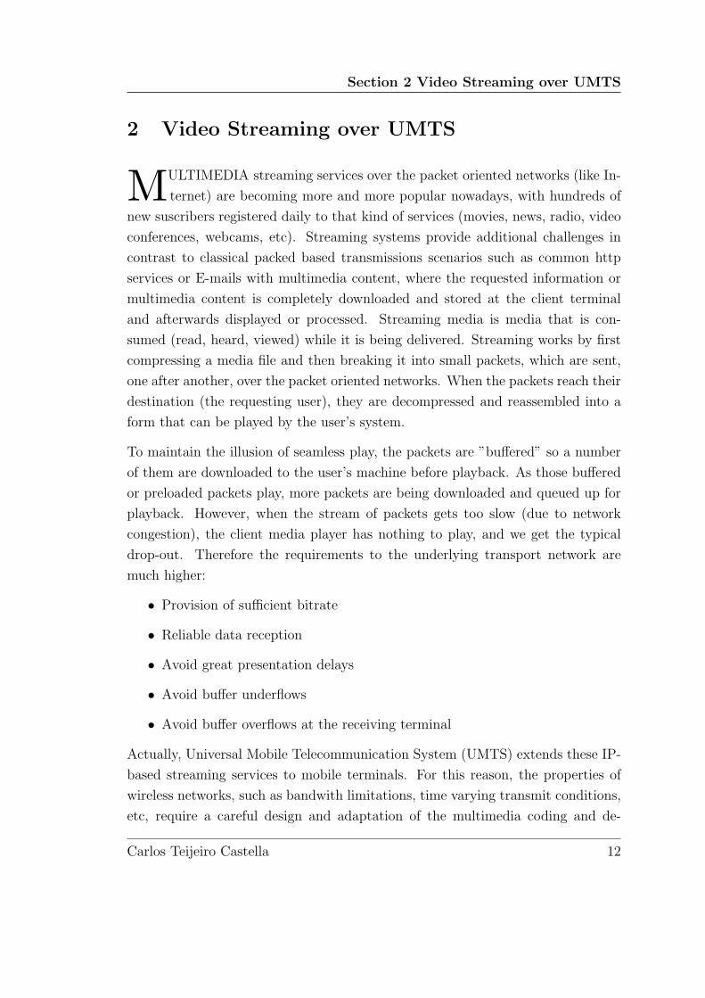
In H.264/AVC, two types of intra predictions are employed: 4×4 Intra predic-

tion and 16×16 Intra prediction. Figure 10 illustrates the nine modes of 4×4

Intra prediction, including DC prediction and eight directional modes. As shown

in Figure 10, only neighboring pixels of the current block contribute to the pre-

diction. For 16×16 Intra prediction, four modes are defined in terms of four

directions.

Figure 10: Intra prediction for a 4×4 block in H.264/AVC

4.2 GoP Level

Due to the spatio-temporal prediction the image distortion caused by a missing MB

is not restricted to that MB itself. Since the spatially or temporally neighboring

macro-blocks are dependent on the damaged MBs, the image error propagates to

temporally neighboring MBs within the video sequence until the next I-frame is

decoded, that means until the next GoP, and to spatially neighboring MBs within


4.3 Cross-Layer Error Detection

the video sequence until the end of the slice. If we use a big sizes of GoP we can

compress better, but the error can propagate over more frames (see Figure 11).

Figure 11: Spatial and temporal error propagation over the GoP

4.3 Cross-Layer Error Detection

Each UDP packet contains a CRC information. If the CRC fails, the whole UDP

packet is discarded. A UDP packet usually represents a slice of the video, like it

is shown in Section 3.3, that means a rather large part of the picture and its loss

results in considerable visual perceptual quality distortion. However, as explained

in Section 2.1, the UMTS stack provides the RLC layer with another CRC checking

the smaller packets. By that Cross-Layer we have the possibility of a finer error

detection. To enable the usage of RLC CRC information we need to pass this

information to the application layer (video codec), then, in order to use cross-

layer detection, the exchange of information between the application and data

link layer is necessary. In our case, the change needed for that is implementation

specific (does not violate the standards). There is also UDP-Lite Protocol [20],



which is similar to the UDP, but can also serve applications in error-prone network

environments that prefer to have partially damaged payloads delivered rather than

discarded. Having the RLC CRC information at the video decoder, the position

of the first erroneous RLC packet within the slice can be specified. Furthermore,

all correctly received RLC packets before the first erroneous one can be decoded

successfully as shown in Figure 12.

That method does not add any computational complexity or data overhead. Due

to the desynchronization of the VLC after the first error within the slice, it is

not possible to use successive RLC packets although the might have been received

correctly, because the start of the next VLC code word within the segment of the

bitstream is not known. Again, a combination with synchronization marks can be

beneficial [18]

Figure 12: Propagation of the error in a slice


Pagina en blanco

Section 5 Distortion

5 Distortion

IN scientific literature [9] it is common to evaluate the quality of reconstruction

of a frame F analyzing its peak to signal-to-noise ratio (PSNR). There are

different ways of calculating PSNR. The problem lies in the fact that there is not

an unified criterion on the way it is calculated. The criteria than we choose to

evaluate the quality of reconstruction of a frame and wich concealment method is

used are shown in this Section.

5.1 Distortion metric

The most common is to get only the luminance component of YUV color space

but a lot of papers not even specify what PSNR have they obtained.

JM10.1 Reference Software outputs PSNR for every component c of the

YUV color space (Y-PSNR, U-PSNR, V-PSNR) for every frame k

PSNR(c)k = 10 · log10

2552

MSE(c)k

[dB], (1)

MSEck being mean square error for the component we are calculating PSNR for.

It is defined as

MSE(c)k =

1

M ·N

N∑i=1

M∑j=1

[F(i, j)− Fo(i, j)]2, (2)

where N ×M is the size of the frame and Fo is the original frame (uncompressed

and not degraded).

JM10.1 also calculates the averages over all the frames for the luminance

and the chrominances

PSNR(c)av =

1

Nfr

Nfr∑k=1

PSNR(c)k , (3)

where Nfr is the number of frames. However, averaging over logarithmic val-

ues (dB’s) is not correct and therefore we have calculated PSNR average as fol-


5.2 Error concealment

lows

PSNRav = 10 · log10

2552

MSEav

[dB], (4)

MSEav being defined as

MSEav =1

3 ·M ·N ·Nfr

3∑c=1

N∑i=1

M∑j=1

Nfr∑k=1

[F(c)k (i, j)− F

(c)o,k(i, j)]

2 (5)

To describe the distortion we are using the Mean Square Error (MSE) instead

of the typical PSNR, because MSE is an additive method, and with that we can

predict more than one error per GoP. We obtain three different values of MSE

from the simulations, one of luminance (Y-MSE) and two of chrominance (U-MSE

and V-MSE). To work with only one value the MSE (2) metric averaged over the

colors is used.

MSEk =1

3

3∑c=1

[MSE(c)k ] (6)


The missing parts of a picture have been concealed with the Copy&Paste error

concealment method. ”Copy&paste” is the simplest temporal error concealment

method [9]. The missing blocks of one frame Fn are replaced by spatially corre-

sponding blocks from the previous frame Fn−1

Fn(i, j) = Fn−1(i, j) (7)

This method only performs well for low-motion sequences but the advantage lies

in its low complexity, requiring a low load of CPU and less time for concealment,

due to the fact that there is no decoding necessary, but only copying MB from the

last frame.

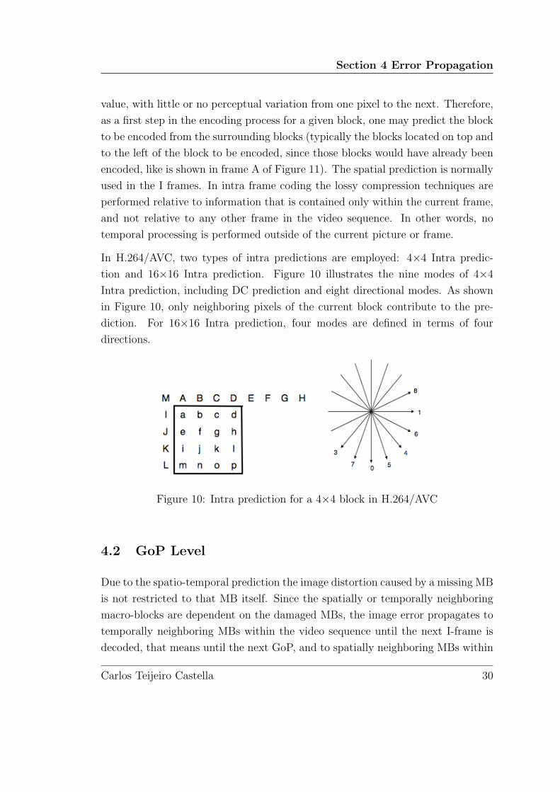
In Figure 13 screenshots of three concealed videos are shown. The first column

illustrates the videos without any error, the second column presents the same

videos with the lost packet without concealment method applied, and the last

column shows the videos with the error concealed by the copy&paste method.


Section 5 Distortion

Figure 13: Conceal method Copy-Paste

The first video, called ”Akiyo”, consists of a newsmoderator speaking in front

of a camera. The sequence is rather static, so the concealment performed very

good due the low motion in the sequence and the resemblance between the frames.

The second video, called ”Foreman”, consists of a foreman speaking to the camera

wich is slightly moving, with irregular movements and a scene change in the second

half of the sequence. In the concealed version we can see than the foreman have

two couples of eyebrows due the movement of his head between the current and

previous frame. Even so the concealed version is very good and that error is not so

critical for the viewers. However, in the third video, called ”Videoclip”, we have

a videoclip sequence with a lot of movement and changing scenes, and that is a

serious problem for the copy&paste concealment method. An example is shown



on the concealed version of the error in the video ”Videoclip”. The concealment

method just copies the MBs of the previous frame, as the previous frame belongs

to another scene, the result is quite annoying for the users.


Section 6 Modeling of Distortion

6 Modeling of Distortion

IN this section we analyse the main factors are influencing the distortion caused

by a packet loss. The distortion is characterized by the size of the distortion

area (spatial and temporal distortion, both commented in Section 4), because if

the error happens in the beginning of a GoP or slice it will be bigger than it

happens in the end, and characterized too by the size of the difference to the

original (compression distortion), because if we want to compress more, we need

to discard more data.

To analyse the main factors of the distortion we assume the usage of the cross-

layer detection described in Section 4.3 and concealment of the lost packets by

copy&paste method introduced in Section 5.2.

6.1 First erroneous RLC packet in slice

One of the most important factors is the first erroneous RLC packet in the slice,

because it determines which part of the slice we can not recover anymore. The size

of the distortion is given by the lost RLC packets, i.e, the number of RLC packets

until the end of the slice. In Figure 14, the importance of the number of lost RLC

packets until the end of the slice is shown. The graphic represent an error in the

same video, same GoP, and the same slice, but the blue line shows the error of an

RLC packet in the beginning of the slice and the red line shows the error of RLC

packet at the end of the slice.

A screenshot of video demonstration about that graph is shown in Figure 15. The

first video caption is represented in the distortion graph by the blue line and the

second video caption is represented by the red line. In the first caption the RLC

packet error is in the beginning of the slice and that causes the discard of the

whole slice. The second caption has the error in the last RLC packet of the slice,

showing how important is the position of the erroneous RLC packet when we are

using the cross-layer detection, because, like we comment in Section 4.3, we can

decode all the slice until the RLC packet error. Without cross-layer detection the

UDP packet (the whole slice) is discarded without any importance of the place of


6.2 Frame number with the erroneous RLC packet

0 5 10 15 20 25 300

20

40

60

80

100

120

Frame

MS

EError RLC in the beginning of Slice

Error RLC in the end of Slice

Figure 14: Importance of the position of the erroneous RLC

the erroneous RLC, and then any error will be treated like the first caption.

Figure 15: Importance of the position of the erroneous RLC

6.2 Frame number with the erroneous RLC packet

Another factor is the position of the frame with the erroneous RLC packet within

the GoP. If we have an error in the beginning of the GoP it propagates until the

end of the GoP. That factor is important also because we introduce an error in



one RLC for every GoP, but the same RLC error does not mean the same frame

position for every GoP. We need to store the exact position to have information

about the error propagation. That is necessary for the prediction later. Figure 16

shows the different frame positions within the GoP of the same RLC error. In

that case we are making an error in the RLC number 600 in every GoP of the

”Foreman” video (Table 5 show how many RLCs per GoP has this video), and the

error start in frame 17 for the first GoP, in the frame 16 for the second GoP and

in the frame 14 for the third GoP. That is because sometimes we can compress

the information better and sometimes we can compress worse. Aside from the

RLC packet error, which error is the most clearly value in the graph, we have a

residual errors during all the video. That values of error in the distortion measure

are about the compression error of the video. We gonna talk about that ahead in

this same section. Note that in the third GoP the residual error disappears in the

end of the frame 20, that is why the video only have on 100 frames, then, in the

third graph, we only can measure 20 frames.

0 5 10 15 20 25 30 35 400

5

10

15

20

25

30

35

Frame

MS

E

GoP 1

GoP 2

GoP 3

Figure 16: Position of the Frame with the RLC error within the GoP

6.3 The average size of the error

The average size of the erroneous MB in bytes is another influencing factor in the

final distortion, because it is not the same to loose one RLC packet containing

one MB and with ten MBs, big sizes of MB means more data, like changing scene,


6.4 Discard encoding/compression errors

more movement, hight detail, etc. It is interesting for us, too, the size of the MB,

to define what kind of video we are decoding. The histograms in Figure 17 show

the nature, the character of all the video sequences used in our simulations. For

example, the ”Fussball” video has higher size values than the others, because the

”Fussball” video contains a panning of the camera and fast movement of several

objects (players, ball,etc).

Figure 17: Average size of the erroneous MBs

6.4 Discard encoding/compression errors

At last, it is important for us to discard the effect of the compression error in

the distortion measure, because we are only interested in influences of the loses,

not of the compression, there are already models for the compression loses [21]

[22]. To facilitate this we only substract the MSE values of the video without

packet looses to the MSE values of the video with packet looses to obtain only the



measure of the transmision error. Figure 18 shows three graphs. The first one is

the distortion measure of a sequence with an erroneous RLC packet. The loss of

an RLC packet is clear, but we already have a residual distortion during all the

sequence, that is caused by the lossy compression. The second graph is a decoded

sequence without RLC packet errors, and that one shows only the compression

error. Then we substract that values from the values of the first graph an obtain

only the distortion of the RLC packet error. The results are shown in the third

graph.

0 5 10 15 20 25 30 35 400

10

20

30

40

Frame

MS

E

0 5 10 15 20 25 30 35 400

10

20

30

40

Frame

MS

E

0 5 10 15 20 25 30 35 400

10

20

30

40

Frame

MS

E

GoP 1GoP 2GoP 3

GoP 1GoP 2GoP 3

GoP 1

GoP 2

GoP 3

Figure 18: We discard encoding/compression errors


Pagina en blanco

Section 7 Simulations Setup

7 Simulations Setup

IN this Section the assumptions than we apply for our project are introduced,

as the modifications made in the source code to achieve our purpose. At the

end of the section how we archieve and process the obtained data is shown.

7.1 Assumptions

To evaluate the performance and influence of the erroneous RLC packet, selected

but representative simulations have been performed. In Table 2 the chosen se-

quences (Foreman, Fussball, Limbach and Videoclip) and the parameters of all

the videos are presented.

To make our simulations, we assume sending the video content over the UMTS

network to be reproduced in a mobile telephone display. Therefore, we have a lim-

itation of the display screen size; the usual format used for the mobile terminals

is QCIF resolution (176×144 pixel). We assume encoding by H.264/AVC because

this is very promising video standard and there are already several devices support-

ing it on the market. We reduce the bandwith needed by the videos decimating

by four their frame-rate, obtaining in this way a 7.5 fps videos, which are better

to stream in wireless networks like UMTS. We do not use the B frames, applying

then an IPPPP.... structure. This is to reflect the base profile of H.264, which

does not necessarily support B frames. The I frame refresh rate is 5.5 seconds,

this results in I frame distance of 40 frames which is a good compromise between

the random access and refresh frequency and compression efficiency. We do not

use data partitioning (DP) and. An RLC-PDU of 320 bits is used, as commented

in Section 2.1.

Concerning the slicing method we chose to fix the maximum number of bytes

per slice among all the slicing methods introduced in Section 3.3. We fix the

maximum size of slices to 650 bytes. Thus, the maximum number of RLCs per

slice (see equation 8) in our case is 17:

Number of RLCs per slice =Slice size [bytes]

RLC size [bytes]. (8)


7.1 Assumptions

Video Content characteristics

Foreman Length Frames Resolution Frame-rate I frame interval

video 13.3 sec 100 176x144 7.5 5.5 sec

Content description: standard test video sequence with one

continuous scene change in the second half of the sequence.

Contains a foreman speaking to the camera wich is slightly

moving or static, after the scene change building in construc-

tion is shown

Fussball Length Frames Resolution Frame-rate I frame interval

video 10 sec 75 176x144 7.5 5.5 sec

Content description: soccer game with a horizontal panning

wide-angle of the camera, following the movement of several

objects (players, small ball,etc.)

Limbach Length Frames Resolution Frame-rate I frame interval

video 3.6 sec 27 176x144 7.5 5.5 sec

Content description: Low motion sequence of a landscape vil-

lage with a slow horizontal panning of the camera and without

dynamic objects.

Videoclip Length Frames Resolution Frame-rate I frame interval

video 14.4 sec 108 176x144 7.5 5.5 sec

Content description: music videoclip sequence with a lot of

movement and changing camara movement between panning

of the camera and static scenes. Separated by scene cuts and

transitions.

Table 2: Content of the sequences



The chosen slicing method is the most suitable one for wireless networks (like

UMTS) because of its limited size in bytes that can be chosen in efficient way to

ease the mapping on the lower layer protocols. Figure 19 shows a graph from the

3GPP technical report 25.322 [7], investigating the overhead caused by different

packet sizes. Blue color indicates the size of packet we decided to use. We fix the

maximum size of the slice to 650 bytes. When using large packets (≥ 650 bytes)

the header overhead is 3 to 5%.

Figure 19: RTP payload vs. headers overhead (3GPP TR 26.937)

All these assumptions were taken into account in order to setup the encoder to

encode the simulations videos.

7.2 Changes to the Joint Model Code

For our simulations we use the Joint Model H.264 [12] version 10.1. This software

is free available to the user without any license fee or royalty. Generated by the

JVT this software is composed by a H.264/AVC video encoder and decoder, and

all the source code is included in the package. We do not modify the encoder, but

we use it to generate the RTP video streaming. We introduce the assumptions

commented in Section 7.1 in the configuration file of the encoder to obtain the

video stream (Table 3 shows the main parameters seted of that configuration file).

The decoder has another configuration file, but is less complex than the encoder’s

case. We only need to indicate which video stream we want to decode, which



concealment method we want to use and set the NAL mode to RTP packets. Both

configuration files, encoder and decoder, are shown in the appendix.

FrameRate = 7 Frame Rate per second (0.1-100.0)

SourceWidth = 176 Frame width

SourceHeight = 144 Frame height

IntraPeriod = 40 Period of I-Frames (0=only first)

NumberBFrames = 0 Number of B coded frames inserted

SymbolMode = 0 Entropy coding method: 0=UVLC, 1=CABAC)

OutFileMode = 1 Output file mode, 0:Annex B, 1:RTP

PartitionMode = 0 0: no DP, 1: 3 Partitions per Slice

SliceMode = 2 1=fixed MB in slice, 2=fixed bytes in slice

SliceArgument = 650 Arguments to modes 1 and 2 above

Table 3: Important values changed in the configuration file of the encoder

When all the parameters are introduced in the configuration file we execute the

encoder software to obtain the RTP stream of the video with the specified charac-

teristics. That stream will be the input of our modified decoder software. Modified

because we introduce new characteristics to the source code of that decoder in or-

der to obtain the required outputs to achieve our purpose, i.e. to insert errors into

RLC packets in the stream, to handle the losses and to obtain the information

about the stream structure necessary for the predictor design as will be shown

later.

We are interested in the CRC on the RLC packets, commented in Section 4.3, and

the lowest transmission layer of the Joint Model (JM) is the Network Abstraction

Layer (NAL). Each syntax structure in H.264/AVC is placed into a logical data

packet called a NAL unit. All NAL units following the first I frame (IDR) have a

slice or a type of data partitioning. In Section 7.1 no usage of data partitioning is

assumed, thus every NAL unit represent a whole slice, and every slice is one part

of the bitstream in the Joint Model, with VLC synchronized at the beginning. The

RLC layer is a data link layer. We modify the JM to segment the bitstream of the

decoder into RLC packets.



7.2.1 Bitstream segmentation in RLCs

To segment the bitstream we only modify the function ”decode one slice” in the

JM. That function is inside the image.c file, in the decoder source code. As Figure

20 shows, the operation of the function is only to decode one slice, as its name

indicates, starting to read an MB from the bitstream and calling the function

”decode one macroblock” to generate the end video file until the flag ”end of slice”

get the value ”TRUE”, and then the function starts with a new slice, making

the same process until the end of the video. If we have any problem reading

the information of the MB (loss of data or erroneous bits), the decoding of that

MB does not happen and we apply an error concealment method, explained in

Section 5.2. Then, we implement the segmentation of the bitstream in RLCs for

that version of the JM (the bitstream inside that function is the bitstream of one

slice), obtaining a new variable with the number of RLCs per slice which will be

important further on in the develop of this project.

Figure 20: Block diagram about function decode one slice

7.2.2 Generate an error in one RLC per GoP

As explained in Section 6 we are interested in the distortion caused by a packet

loss, specifically in an RLC packet loss. Then we need to modify the JM to

generate that losses. That modification is performed in the same function as the

segmentation, because now we have the bitstream segmented in RLCs and we can

identify better the position of one RLC. It is important to find the exact position

of an RLC packet because we want to generate an error (packet loss) in every



possible RLC packet position in all the GoPs inside the video sequence. Then we

need to make one simulation for every possible RLC packet per GoP, and that

means a lot of hours of video decoding (shown in Table 4). That time is obtained

running the simulations on a Intel with a 2GHz CPU and 768MB of RAM.

Video RLCs/GoP seconds/simulation Total time

Foreman 1824 29 52896

Fussball 2835 32 90720

Limbach 1009 7 7063

Videoclip 2594 37 95978

Total simulation time 68,5 hours

Table 4: Time of simulations per video

Of course every GoP does not have the same number of RLCs, but to make all

the simulations automatically we need to use the highest number of RLCs of the

video to simulate all the possible errors. For example, the Foreman video has 1330

RLCs in the first GoP, 1824 RLCs in the second GoP and 754 RLCs in the third

one (data shown in the Table 5). That only means that the third GoP does not

have any error from the RLC 754 until the RLC 1824 in the simulation, and the

first GoP does not have any error from the RLC 1330 until the RLC 1824, because

they do not have so much RLCs, due the information contained in the GoP and

because sometimes the information is compressed better, and sometimes worst,

depending of video sequence characteristics. In the third GoP the difference of

RLCs is so big because the third GoP in the Foreman video only have 20 frames,

because is the final of the video (explained in Figure 16), and the size of the other

GoPs is 40.

Video GoP1 GoP2 GoP3

Foreman 1330 RLCs 1824 RLCs 754 RLCs

Table 5: RLCs per GoP in Foreman video

The first modification in the JM to generate the error is to found the exact RLC,

and then, the second one, is discard the selected RLC packet to generate the packet



loss. To discard a packet we only avoid the decoding process for the selected packet

and we apply conceal in from that region until the end of the slice.

7.2.3 Error input by command line

Another modification of the JM was the error input. To make the acquisition of

the MSE values of every RLC position for every video more easier and polite, we

modify the JM to introduce the error patern by the command line. Then it is not

necessary to re-compile the JM every time we need to change the error pattern,

because it is not inside of the code. Furthermore, with that change, it is more easy

to make a script to generate all the RLC errors of one video automatically. Then,

to execute the decoder we need to put, moreover, the number of the erroneous

RLC packet.

Then, the normal decoder work with the next parameters:

ldecod.exe <Configuration file>

Example:

ldecod.exe decoder.cfg

And our modified version have this input parameters:

ldecod.exe <Configuration file> <RLC error number>

Example:

ldecod.exe decoder.cfg 300

7.2.4 Bitstream structure generator

Then, another modification to the code was necessary to collect all the information

about the video to process it later with Matlab (explained with detail in Section

7.3). We need to collect the exact position of the erroneous RLC packet and

all the important information related to its, like the important factors explained

in Section 6. The Table 6 shows wich values we chose to define the bitstream

structure of the video.

We introduce the modifications in the function ”decode one slice”, inside the file



Group of Pictures number Current RLC packet

Frame number within the GoP Current MB number

Slice number Size of the slice

Table 6: Extra values shown in the output of the video

image.c of the JM code, taking advantage of the changes applied before to segment

the bitstream in RLCs, explained in Section 7.2.1.

To collect all the information we need to introduce changes in two different levels

of the function ”decode one slice”, in the slice level and the MB level. In the slice

level we take the values of the whole slice, because we don’t know some values

until the end of itself. Then, here, in the slice level, we take the total number

of RLC packets per slice and the total numbers of MB per slice. Further on the

function ”decode one slice” we go inside of the MB level, because we start to read

the slice and to decode the MB inside of the slice. Then, in this level, we take

the values of the current RLC packet number within the GoP and current MB

number. It is about that than we need to make two different index to differentiate

from wich level come the information. Table 7 shows all the values taken from the

two different levels.

Slice level MB level

Index Index

GoP number GoP number

Frame number Frame number

Frame number in GoP Frame number in GoP

Slice number Slice number

Size of the slice Size of the slice

Num. of RLC packets in the slice Current num. of RLC packets in the GoP

Num. of MBs in the slice Num. of MBs in the RLC packet

Average MB size in the slice Num. of RLC packets until the slice end

Table 7: Values of the different levels

That modifications are only a output values to generate a file with all the informa-

tion of the video. At the end of the decoding process we obtain a text file with two



different indexes and with all the structure information about the video bitstream.

Figure 21 show a piece of the structure of Silent video stream. That screenshot

shows a whole slice, with the index ”-2” the MB level is identified and with index

”-1” the slice level. Then we process that structure jointly with the MSE values

of all the RLC packet errors of Silent video in Matlab (see Section 7.3).

Figure 21: Example of output file with the bitstrean structure

7.3 Matlab process

In order to analyse and arrange the data obtained from all the simulations (re-

member than we have thousands of files, one file for every possible RLC packet

error and for all the videos), we decided to use the Matlab software. The inten-

tion is to generate a table with every possible postion of RLC packet error and

then to associate each cell of the table with the corresponding MSE value. As

is explained in Section 7.2.4, we need a data structure to find the exact place of

every erroneous RLC packet, because the place is not the same for every video or

sequence. The reason is the changing content of the videos, resulting in different

compression efficiency that leads in different slice sizes and then different RLC

positions. Therefore we need the MSE value of every RLC packet error and the

structure of the video to locate the RLC packet inside the video.

Then, as Figure 22 shows, the input of the Matlab process , for every video, are the

thousands of files with the MSE values and the information about the structure

of the video. Both inputs are generated by the modified JM H.264 decoder.


7.3 Matlab process

Figure 22: Schema of the process to get the input files for Matlab

First of all we take all MSE values an we make an average of the YUV components

MSE, obtaining an unique value for every frame in the simulation. Then we

substract the encoding/compression error in the distortion measure, as commented

in detail in Section 6.4. From this point we are only working with the MSE caused

by the error, and not with the normal MSE value obtained from the simulations,

containing the compression artifacts.

We organize the MSE values in function of the important factors commented in

Section 6. To achieve that purpose we generate a 4D matrix with the important

factors as an index.

Parameters of the index:

• Number of the erroneous frame within the Group of Pictures: Obtained

from the input file with the structure of the video, searching the RLC packet

number error, and getting then the frame number within the GoP. The value

can vary from 1 until 40, the maximun number of frames per GoP.

• Number of RLC packets until the end of the slice: Obtained from the input



file with the strucutre of the video. For us the number of the slice is not

so important, but rather the position within the slice. If the RLC packet is

located at the beginning of the slice the error will be bigger than the same

RLC packet is located at the end of the slice, as commented in Section 6.1.

The value can vary from 1 until 17, because the maximun slice size is 650

bytes, and the size of the RLC payload is 40 bytes.

• Average size of the erroneous MBs: The erroneous area is divided by the

erroneous MBs, obtaining in this way the average size of the erroneous MBs.

Because it is not the same to have an error in MB with a lot of information,

bigger in bytes size, than another one with low information value and smaller

size in bytes. Than, we perform a classification of the sizes of the MB. Figure

23 shows such classification, generating nine groups. Every group has a size

of 5 bytes except of the last group, wich is the I group, formed by MBs with

a size bigger than 40 bytes. Thich value is not the most typical in the videos,

as shown in Figure 23. Then, the maximun value for us in that field is 40.

• Number of frame with the MSE Value: Here all the MSE values of the GoP

are saved, from the frame 0 until the frame 39, whenever the RLC packet

error and average error MB size agree with the other values of the index.

Then, the value registered here correspond to frames 1 until 40, maximum

number of frames per GoP.

The 4D matrix is generated for all the four different videos of our simulations.

Every matrix has more than one million of elements. All the four matrices are

averaged and saved in a new matrix, with all the values of all the videos. In

this way we obtain a kind of look-up table function with an MSE value for every

possible position of error. In other words, if we have all the information of the

video, that function can work like a predictor, telling us wich importance have

every possible RLC packet loss.


7.3 Matlab process

Figure 23: Association of erroneous MBs in Matlab by size.


Section 8 Performance Evaluation

8 Performance Evaluation

IN Figure 24 the prediction error measurement setup is presented. First, a new

video sequence is decoded in our modified JM decoder, an random error is

introduced as is comented in Section 7.2.3. To obtain the predicted MSE, we found

a position in our structure (now a predictor) with that error pattern, wich means

the four parameters commented in Section 7.3, obtaining predicted distortion.

After the decoding, resulting MSE is compared with the predicted value, making

a correlation of both MSE vectors to evaluate the fidelity of that prediction.

Figure 24: Evaluation of prediction performance

In this chapter, the prediction performance of our distortion model is tested and

evaluated with new and included videos of the original set. First we evaluate the

performance of our predictor (its consistency) with the same four videos which

were used to obtain the look-up table function. In Figure 25 the characteristics

of all the videos included in the look-up table function are shown. That graph

search all the errors in the video of our simulations and represent the MSE values

arranged by the total erroneous RLCs in the slice and how many MBs are inside

that erroneous RLCs. As is clearly shown in the graphs, the values tend to by

higher when the error affect a bigger number of MBs. But not always in the same

way. For example, in the Fussball sequence the higher values of MSE does not

happen with the biggest number of MBs involved in the error, that is why the

characteristics of the video. A very high motion video with several objects in

movement(as Table2 shows), then, a lot of the MB are intra decoded, because is


too much information to predict it, and the motion vectors does not have enough

information about all the MB due the fast movement of the objects and the panning

of the camera. In the case of Videoclip sequence, the strange results of the graph

can be caused by the constant scene change. That four graphs prove than the 4

videos are very different in contents and in structure. In spite of everything the

results are satisfactory.

Figure 25: MSE value of the lost number of RLCs depending the contained MBs

In Table 8 the results of the correlation are shown. Very good results always over

the 0,9 of correlation were obtained. We can observe than the worst result is

produced in the Fussball video, due to its characteristics. As is explained in Table

2, the Fussball video is a very high motion video, with panning of the camera

and a several objects in movement, in this case the players and the ball, and that

causes a difficult to obtain a prediction.

Video MSE Correlation

Foreman 0,9598

Fussball 0,9189

Limbach 0,9591

Videoclip 0,9589

Table 8: Correlation between predicted MSE and the real distortion measure

Table 8 only have a correlation between the same videos included in the original

set used to obtain that look-up table function. However, the most interesting

evaluation for us is to check the prediction performance with another video not used



to obtain the look-up table function. In that case we will confirm if the predictor

can provide correct distortion estimation for any video. For that evaluation we

choose a sequence called Silent. As Table 9 shows, the encoding characteristics of

Silent video are the same than the other videos (see Table 2), wich ones are the

typical in UMTS network video transmissions, like is commented in Section 7.1,

but the video have a different content in comparison to any video used to generate

the predictor.

Video Content characteristics

Silent Length Frames Resolution Frame-rate I frame interval

video 9.9 sec 74 176x144 7.5 5.5 sec

Content description: sequence without any scene change,

with a static camera recording a woman talking in the sign

language. The background is static, but the the arms move-

ment of the woman is quite fast.

Table 9: Content of the Silent sequence

Figure 26 shows the characteristics of the Silent video. We can observe than the

MB in the silent video does not have a big content of information, due the low

motion content wich cause than we need lees information to codify the whole frame.

We can check this in the top-left area of the graphic. There we can found some

errors of big MBs, but the MSE value is very low, determining the less importance

of that big MBs in that video. Next to Silent graphic we can found an average

graphic of all the videos included in the look-up table function. We can observe

than the predictor (average graphic) really fit with the Silent video values, maybe

we only have a little difference in high error distortion values wich affect the bigger

part of the frame, that is represented in the top-right corner of the graphic.

To make the evaluation of the Silent video we prefer to use the PSNR value of

the distortion measure, due the more resemblance with the human eye behaviour.

For the reason that, as is explained in Section 5.1, the MSE distortion measure is

additive and it was interesting for us in way to predict more than one error per

GoP, but in that evaluation we are making only one error to test the correct use of

the parameters and check the predictor, then, the evaluation is more conclusive if


Figure 26: Characteristics of Silent video and the Average of the predictor videos

we use PSNR instead of MSE values. In any way both cases are shown in Figure

27 with a very good approximation of the predictor to the real curve in any case.

In the PSNR graph the values does not appear until frame number 5, thats why

the capture was taked for an example with an RLC packet error in frame number

5, that means than the sequence does not have any error before, and PSNR tend

to infinite when does not found any error, and it is about that than the values

does not appear.

The evaluation performance with the video not used to obtain the look-up table

is shown in Table 8. To obtain the value of PSNR correlation of Silent video

we discard the infinite values (wich we explain in the paragraph before), due the

mathematic problems it involve to calculate the correlation. Then we use, for that

exemple (see Figure 27), only the values from the frame 5 until the last frame of

the GoP, the frame 40. That causes a little bit decrease of the correlation value,

but in any case the value demonstrate the good performance of our predictor and

better ressemblance with the human eye of the PSNR values, obtaining a better

correlation in front of MSE values.

Mode Correlation

MSE 0.9621

PSNR[dB] 0.981

Table 10: Correlation of the Silent video



Figure 27: Evaluation of prediction performance


Pagina en blanco

Section 9 Conclusions

9 Conclusions

The aim of this thesis is to propose a rate-distortion model for H.264/AVC encoded

video stream with QCIF resolution. The model assumes a cross layer information

exchange between the radio link layer (RLC in UMTS) and the transport layer in

a mobile communication system UMTS. Thus, apart from the UDP layer CRC,

the CRC information from RLC packets can be used for error detection within the

blocks smaller than the whole UDP packet. The RLC blocks without error can

then be detected until the first error occurs. After the first error occurs, the VLC

desynchronizes and therefore, an error concealment routine is called to interpolate

the errors.

To obtain the model, we analyzed several parameters influencing the distortion

at the decoder. We chose the size of the lost part of the slice in bytes and in

macroblocks as well as the position of the error within the group of pictures. We

performed decoding for all possible positions of an RLC error for chosen video

sequences. The video sequences were selected to cover various types of movement,

scene changes and amounts of spatial information. By averaging over the sequences

and the errors with the same number of bytes, macroblocks and position without

the GoP, we finally obtained a look-up table allowing for prediction of the distortion

based on those parameters only.

In the last part of the thesis we test the consistency of this data set by testing its

distortion estimation performance for the sequences included in the model. The

correlation with the model is about 95%. To test the estimation performance, we

also compare the estimated distortion with the distortion in new sequences, that

were not used to form the model. The correlation about 96,2% for MSE and 98,1%

for PSNR was obtained.

The fairly well correlation could possibly even be increased by using the informa-

tion about the size of motion vectors, as the distortion does not only depend on

the size of the lost packets but also on their content. And the size of the content

may be high or low because of the residuals or because of the motion vectors.

These two cases, however may result in different amount of distortion.

The proposed model can be surely used for better scheduling and priority handling


in the networks as it allows for predicting the importance od the lost packets

without having to decode them.


REFERENCES

References

[1] Third Generation Partnership Project (3GPP), avaliable at http://www.3gpp.org.

[2] H. Holma, A. Toskala, ”WCDMA for UMTS: Radio Access For Third GenerationMobile Communications,” John Wiley & Sons, Ltd, UK, 2004.

[3] JVT ”Draft ITU-T recommendation and final draft international standard of jointvideo specification (ITU-T rec. H.264– ISO/IEC 14496-10 AVC),” March 2003, JVT-G050 available on http://bs.hhi.de/ wiegand/JVT.html. )

[4] ITU-T Recommendation H.263, Video codec for Low Bit Rate Communication, Jan-uary 2005.

[5] ISO/IEC JTC1/SC29/WG11 N4030, Overview of the MPEG-4 Standard, March2001.

[6] T. Wiegand, G.J. Sullivan, G. Bjontegaard,A. Luthra, ”Overview of the H.264/AVCVideo Coding Standard,” IEEE Transactions on Circuits and Systems for VideoTechnology, vol. 13, no. 7, pp. 560-576, July 2003.

[7] 3GPP TSG TR 25.322, ”Radio Link Control (RLC) protocol specification,” v.4.12.0,June 2004.

[8] 3GPP TSG TR 25.212, ”Technical Specification Group Radio Access Network,”v.6.7.0, December 2005.

[9] M.T. Sun, A.R. Reibman, ”Compressed Video over Networks,” Signal Processingand Communications Series, Marcel Dekker Inc., New York, 2001.

[10] 3GPP TR 26.937 ”Transparent end-to-end packet switched streaming service (PSS);RTP usage model” V5.0.0, September 2003.

[11] O. Nemethova, J. Canadas, M. Rupp, ”Improved Detection for H.264 EncodedVideo Sequences over Mobile Networks,” ISCTA 2005, Ambleside, UK, 2005.

[12] H.264/AVC Software Coordination, ”JM Software,” ver.10.1, available inhttp://iphome.hhi.de/suehring/tml/.

[13] RFC 1889, ”RTP: A Transport Protocol for Real-Time Applications”.

[14] RFC 3984, ”RTP Payload Format for H.264 Video”.


REFERENCES

[15] 3GPP TSG-Terminals. ”Common Test Environments for UE Conformance Testing”3GPP TS 34.108 v 3.4.0.

[16] RFC 0768 ”UDP:User Datagram Protocol”.

[17] RFC 0791 ”IP: Internet Protocol”.

[18] Olivia Nemethova, Wolfgang Karner, Ameen Al-Moghrabi and Markus Rupp”Cross-Layer Error Detection for H.264 Video over UMTS”, in Proc. of Interna-tional Wireless Summit 2005, Aalborg, Denmark, September 2005.

[19] 3GPP TS 34.108: Common test environments for user equipment (UE). Confor-mance testing (Release 99).

[20] RFC 3828 ”The Lightweight User Datagram Protocol (UDP-Lite)”.

[21] Antonio Ortega and Kannan Ramchandran ”Rate distortion methods for imageand video compression”, IEEE Signal Processing Magazine, Volume 15, Issue 6,November 1998.

[22] Siwei Ma, Wen Gao, Member and Yan Lu ”Rate-Distortion Analysis for H.264/AVCVideo Coding and its Application to Rate Control”, IEEE Transactions on Circuitsand Systems for Video Technology, Volume 15, Issue 12, December 2005.


ANNEXOS TÍTOL DEL TFC: RLC based distortion model for H.264 video streaming TITULACIÓ: Enginyeria Tècnica de Telecomunicació, especialitat Telemàtica AUTOR: Carlos Teijeiro Castellà SUPERVISORA: Olívia Némethová DIRECTOR: Markus Rupp DATA: 23 de juny de 2006

Pagina en blanco

Section A Annex

A Annex

A.1 List of Abreviations

3GPP 3rd Generic Partnership Project

AM Acknowledged Mode

ARQ Automatic Repeat reQuest

AS Application Server

AVC Advanced Video Coding

CABAC Context-Adaptative Binary Coding

CAVLC Context-Adaptative Variable Length Coding

CN Core Network

CPU Central Processing Unit

CRC Cyclic Redundancy Check

DCT Discrete Cosine Transform

DP Data Partitioning

DVB-H Digital Video Broadcasting Handheld

DVD Digital Video Disc

EDGE Enhanced Data Rates for Global Evolution

FMO Flexible Macro Block Ordering

FDMA Frequency Division Multiple Access

GoP Group of Pictures

GPRS General Packet Radio Service

GSM Global System for Mobile communications

HDTV High Definition Television

HSCSD High Speed Circuit Switched Data

HDSPA High speed Downlink Packet Access

IP Internet Protocol

ITU-T International Telecommunication Union - Telecommunication

JM Joint Model

JPEG Joint Photographic Experts Group

JVT Joint Video Team


A.1 List of Abreviations

MAC Medium Access Control

MB Macro Block

MMS Multimedia Messaging Services

MPEG Moving Picture Experts Group

MSE Mean Square Error

NAL Network Abstraction Layer

PDCP Packet Data Convergence Protocol

PPS Picture Parameter Sets

PS Packet Switch

PSNR Peak to Signal-to-Noise Ratio

RAN Radio Access Networks

RAM Random Access Memory

RFC Request For Comments

RLC Radio Link Controller

RNC Radio Network Controller

RTP Real Time Protocol

SPS Sequence Parameter Sets

TDMA Time Division Multiple Access

TTI Time Transmission Interval

UDP User Datagram Protocol

UE User Equipments

UEP Unequal Error Protection

UM Unacknowledged Mode

UMTS Universal Mobile Telecommunication System

UTRAN Universal Terrestrial Radio Access

VCEG Video Coding Experts Group

VLC Variable Length Code

WCDMA Wide Code Division Multiple Access


Section A Annex

A.2 Encoder configuration file : encoder.cfg

# New Input File Format is as follows

# <ParameterName> = <ParameterValue> # Comment

#

# See configfile.h for a list of supported ParameterNames

###########################################################################

# Files

###########################################################################

InputFile = "silent7fps.yuv" # Input sequence

InputHeaderLength = 0 # If the inputfile has a header, state it’s

#length in byte here

StartFrame = 0 # Start frame for encoding. (0-N)

FramesToBeEncoded = 75 # Number of frames to be coded

FrameRate = 7 # Frame Rate per second (0.1-100.0)

SourceWidth = 176 # Frame width

SourceHeight = 144 # Frame height

TraceFile = "silent7fps_enc.txt"

ReconFile = "silent7fps-40intraperiod_rec.yuv"

OutputFile = "silent7fps-40intraperiod.264"

###########################################################################

# Encoder Control

###########################################################################

ProfileIDC = 100 # Profile IDC (66=baseline, 77=main,

#88=extended; FREXT Profiles: 100=High, 110=High 10,

122=High 4:2:2, 144=High 4:4:4, for params see below)

LevelIDC = 40 # Level IDC (e.g. 20 = level 2.0)

IntraPeriod = 40 # Period of I-Frames (0=only first)

EnableOpenGOP = 0 # Support for open GOPs

#(0: disabled, 1: enabled)



IDRIntraEnable = 0 # Force IDR Intra (0=disable 1=enable)

QPISlice = 26 # Quant. param for I Slices (0-51)

QPPSlice = 26 # Quant. param for P Slices (0-51)

FrameSkip = 0 # Number of frames to be skipped in input

#(e.g 2 will code every third frame)

ChromaQPOffset = 0 # Chroma QP offset (-51..51)

UseHadamard = 1 # Hadamard transform (0=not used,

#1=used for all subpel positions, 2=use only for qpel)

DisableSubpelME = 0 # Disable Subpixel Motion Estimation

#(0=off/default, 1=on)

SearchRange = 16 # Max search range

NumberReferenceFrames = 1 # Number of previous frames used

#for inter motion search (1-16)

PList0References = 0 # P slice List 0 reference override

#(0 disable, N <= NumberReferenceFrames)

Log2MaxFNumMinus4 = 0 # Sets log2_max_frame_num_minus4

#(-1 : based on FramesToBeEncoded/Auto, >=0 : Log2MaxFNumMinus4)

Log2MaxPOCLsbMinus4 = -1 # Sets log2_max_pic_order_cnt_lsb_minus4

#(-1 : Auto, >=0 : Log2MaxPOCLsbMinus4)

GenerateMultiplePPS = 0 # Transmit multiple parameter sets. Currently

#parameters basically enable all WP modes (0: diabled, 1: enabled)

ResendPPS = 0 # Resend PPS (with pic_parameter_set_id 0) for

#every coded Frame/Field pair (0: disabled, 1: enabled)

MbLineIntraUpdate = 0 # Error robustness

#(extra intra macro block updates)

#(0=off, N: One GOB every N frames are intra coded)

RandomIntraMBRefresh = 0 # Forced intra MBs per picture

InterSearch16x16 = 1 # Inter block search 16x16 (0=disable, 1=enable)






Section A Annex



IntraDisableInterOnly = 0 # Apply Disabling Intra conditions only

#to Inter Slices (0:disable/default,1: enable)

Intra4x4ParDisable = 0 # Disable Vertical & Horizontal 4x4

Intra4x4DiagDisable = 0 # Disable Diagonal 45degree 4x4

Intra4x4DirDisable = 0 # Disable Other Diagonal 4x4

Intra16x16ParDisable = 0 # Disable Vertical & Horizontal 16x16

Intra16x16PlaneDisable = 0 # Disable Planar 16x16

ChromaIntraDisable = 0 # Disable Intra Chroma modes other than DC

DisposableP = 0 # Enable Disposable P slices in the primary layer

#(0: disable/default, 1: enable)

DispPQPOffset = 0 # Quantizer offset for disposable P slices

#(0: default)

###########################################################################

# B Slices

###########################################################################

NumberBFrames = 0 # Number of B coded frames inserted

#(0=not used)

QPBSlice = 30 # Quant. param for B slices (0-51)

BRefPicQPOffset = 0 # Quantization offset for reference

#B coded pictures (-51..51)

DirectModeType = 1 # Direct Mode Type (0:Temporal 1:Spatial)

DirectInferenceFlag = 1 # Direct Inference Flag (0: Disable 1: Enable)

BList0References = 0 # B slice List 0 reference override


BList1References = 1 # B slice List 1 reference override


# 1 List1 reference is usually recommended for normal GOP Structures.

# A larger value is usually more appropriate if a more flexible



# structure is used (i.e. using PyramidCoding)

BReferencePictures = 0 # Referenced B coded pictures (0=off, 1=on)

PyramidCoding = 0 # B pyramid (0= off, 1= 2 layers,

#2= 2 full pyramid, 3 = explicit)

PyramidLevelQPEnable = 1 # Adjust QP based on Pyramid Level

#(in increments of 1).

#Overrides BRefPicQPOffset behavior.(0=off, 1=on)

ExplicitPyramidFormat = "b2r28b0e30b1e30b3e30b4e30"

# Explicit Enhancement GOP.

#Format is {FrameDisplay_orderReferenceQP}.

# Valid values for reference type is r:reference, e:non reference.

PyramidRefReorder = 1 # Reorder References according to Poc distance

#for PyramidCoding (0=off, 1=enable)

PocMemoryManagement = 1 # Memory management based on Poc Distances

#for PyramidCoding (0=off, 1=on)

BiPredMotionEstimation = 0 # Enable Bipredictive based Motion Estimation

#(0:disabled, 1:enabled)

BiPredMERefinements = 3 # Bipredictive ME extra refinements

#(0: single, N: N extra refinements (1 default)

BiPredMESearchRange = 16 # Bipredictive ME Search range (8 default).

#Note that range is halved for every extra refinement.

BiPredMESubPel = 1 # Bipredictive ME Subpixel Consideration

#(0: disabled, 1: single level, 2: dual level)

###########################################################################

# SP Frames

###########################################################################

SPPicturePeriodicity = 0 # SP-Picture Periodicity (0=not used)

QPSPSlice = 28 # Quant. param of SP-Slices for


Section A Annex

#Prediction Error (0-51)

QPSP2Slice = 27 # Quant. param of SP-Slices for

#Predicted Blocks (0-51)

###########################################################################

# Output Control, NALs

###########################################################################

SymbolMode = 0 # Symbol mode

#(Entropy coding method: 0=UVLC, 1=CABAC)

OutFileMode = 1 # Output file mode, 0:Annex B, 1:RTP

PartitionMode = 0 # Partition Mode, 0: no DP, 1: 3 Partitions per Slice

###########################################################################

# CABAC context initialization

###########################################################################

ContextInitMethod = 1 # Context init (0: fixed, 1: adaptive)

FixedModelNumber = 0 # model number for fixed decision for

#inter slices ( 0, 1, or 2 )

###########################################################################

# Interlace Handling

###########################################################################

PicInterlace = 0 # Picture AFF (0: frame coding,

#1: field coding, 2:adaptive frame/field coding)

MbInterlace = 0 # Macroblock AFF (0: frame coding,

#1: field coding, 2:adaptive frame/field coding)

IntraBottom = 0 # Force Intra Bottom at GOP Period

###########################################################################

# Weighted Prediction



###########################################################################

WeightedPrediction = 0 # P picture Weighted Prediction

#(0=off, 1=explicit mode)

WeightedBiprediction = 0 # B picture Weighted Prediciton

#(0=off, 1=explicit mode, 2=implicit mode)

UseWeightedReferenceME = 0 # Use weighted reference for ME

#(0=off, 1=on)

###########################################################################

# Picture based Multi-pass encoding

###########################################################################

RDPictureDecision = 0

# Perform RD optimal decision between

#different coded picture versions.

# If GenerateMultiplePPS is enabled then this will test

#different WP methods.

# Otherwise it will test QP +-1 (0: disabled, 1: enabled)

RDPictureIntra = 0

# Perform RD optimal decision also for intra coded

#pictures (0: disabled (default), 1: enabled).

RDPSliceWeightOnly = 1

# Only consider Weighted Prediction for P slices

#in Picture RD decision. (0: disabled, 1: enabled (default))

RDBSliceWeightOnly = 0

# Only consider Weighted Prediction for B slices

#in Picture RD decision. (0: disabled (default), 1: enabled )

###########################################################################

# Loop filter parameters

###########################################################################

LoopFilterParametersFlag = 0 # Configure loop filter


Section A Annex

#(0=parameter below ingored, 1=parameters sent)

LoopFilterDisable = 0 # Disable loop filter in slice header

#(0=Filter, 1=No Filter)

LoopFilterAlphaC0Offset = 0

# Alpha & C0 offset div. 2, {-6, -5, ... 0, +1, .. +6}

LoopFilterBetaOffset = 0

# Beta offset div. 2, {-6, -5, ... 0, +1, .. +6}

###########################################################################

# Error Resilience / Slices

###########################################################################

SliceMode = 2 # Slice mode (0=off 1=fixed #mb in slice

2=fixed #bytes in slice 3=use callback)

SliceArgument = 650 # Slice argument (Arguments to modes 1 and 2 above)

num_slice_groups_minus1 = 0 # Number of Slice Groups Minus 1,

#0 == no FMO, 1 == two slice groups, etc.

slice_group_map_type = 0

# 0: Interleave, 1: Dispersed, 2: Foreground with left-over,

# 3: Box-out, 4: Raster Scan 5: Wipe

# 6: Explicit, slice_group_id read from SliceGroupConfigFileName

slice_group_change_direction_flag = 0

# 0: box-out clockwise, raster scan or wipe right,

# 1: box-out counter clockwise, reverse raster scan or wipe left

slice_group_change_rate_minus1 = 85 #

SliceGroupConfigFileName = "sg0conf.cfg"

# Used for slice_group_map_type 0, 2, 6

UseRedundantSlice = 0 # 0: not used,

#1: one redundant slice used for each slice (other modes not supported yet)

###########################################################################

# Search Range Restriction / RD Optimization



###########################################################################

RestrictSearchRange = 2 # restriction for

#(0: blocks and ref, 1: ref, 2: no restrictions)

RDOptimization = 1 # rd-optimized mode decision

# 0: RD-off (Low complexity mode)

# 1: RD-on (High complexity mode)

# 2: RD-on (Fast high complexity mode - not work in FREX Profiles)

# 3: with losses

DisableThresholding = 0

# Disable Thresholding of Transform Coefficients

(0:off, 1:on)

DisableBSkipRDO = 0 # Disable B Skip Mode consideration from

RDO Mode decision (0:off, 1:on)

SkipIntraInInterSlices = 0

# Skips Intra mode checking in inter slices if certain

#mode decisions are satisfied (0: off, 1: on)

# Explicit Lambda Usage

UseExplicitLambdaParams = 0 # Use explicit lambda scaling parameters

#(0:disabled, 1:enabled)

LambdaWeightIslice = 0.65

# scaling param for I slices. This will be used as

#a multiplier i.e. lambda=LambdaWeightISlice * 2^((QP-12)/3)

LambdaWeightPslice = 0.68

# scaling param for P slices. This will be used as

#a multiplier i.e. lambda=LambdaWeightPSlice * 2^((QP-12)/3)

LambdaWeightBslice = 2.00

# scaling param for B slices. This will be used as

#a multiplier i.e. lambda=LambdaWeightBSlice * 2^((QP-12)/3)

LambdaWeightRefBslice = 1.50

# scaling param for Referenced B slices. This will be

#used as a multiplier i.e. lambda=LambdaWeightRefBSlice * 2^((QP-12)/3)

LambdaWeightSPslice = 1.50


Section A Annex

# scaling param for SP slices. This will be used as a

#multiplier i.e. lambda=LambdaWeightSPSlice * 2^((QP-12)/3)

LambdaWeightSIslice = 0.65

# scaling param for SI slices. This will be used as a

#multiplier i.e. lambda=LambdaWeightSISlice * 2^((QP-12)/3)

LossRateA = 10

# expected packet loss rate of the channel for the first partition,

#only valid if RDOptimization = 2

LossRateB = 0

# expected packet loss rate of the channel for the second partition,


LossRateC = 0

# expected packet loss rate of the channel for the third partition,


NumberOfDecoders = 30

# Numbers of decoders used to simulate the channel,


RestrictRefFrames = 0

# Doesnt allow reference to areas that have been

#intra updated in a later frame.

###########################################################################

# Additional Stuff

###########################################################################

UseConstrainedIntraPred = 0 # If 1, Inter pixels are not used for

#Intra macroblock prediction.

LastFrameNumber = 0 # Last frame number that have to be coded

#(0: no effect)

ChangeQPI = 16 # QP (I-slices) for second part of sequence (0-51)

ChangeQPP = 16 # QP (P-slices) for second part of sequence (0-51)

ChangeQPB = 18 # QP (B-slices) for second part of sequence (0-51)

ChangeQPBSRefOffset = 2 # QP offset (stored B-slices) for second



part of sequence (-51..51)

ChangeQPStart = 0 # Frame no. for second part of sequence

(0: no second part)

NumberofLeakyBuckets = 8 # Number of Leaky Bucket values

LeakyBucketRateFile = "leakybucketrate.cfg"

# File from which encoder derives rate values

LeakyBucketParamFile = "leakybucketparam.cfg"

# File where encoder stores leakybucketparams

NumberFramesInEnhancementLayerSubSequence = 0

# number of frames in the Enhanced Scalability Layer(0: no Enhanced Layer)

NumberOfFrameInSecondIGOP = 0

# Number of frames to be coded in the second IGOP

SparePictureOption = 0

# (0: no spare picture info, 1: spare picture available)

SparePictureDetectionThr = 6

# Threshold for spare reference pictures detection

SparePicturePercentageThr = 92

# Threshold for the spare macroblock percentage

PicOrderCntType = 2

# (0: POC mode 0, 1: POC mode 1, 2: POC mode 2)

###########################################################################

#Rate control

###########################################################################

RateControlEnable = 0 # 0 Disable, 1 Enable

Bitrate = 105000 # Bitrate(bps)

InitialQP = 24

# Initial Quantization Parameter for the first I frame

# InitialQp depends on two values: Bits Per Picture,

# and the GOP length

BasicUnit = 11 # Number of MBs in the basic unit


Section A Annex

# should be a fractor of the total number

# of MBs in a frame

ChannelType = 0

# type of channel( 1=time varying channel; 0=Constant channel)

###########################################################################

#Fast Mode Decision

###########################################################################

EarlySkipEnable = 0 # Early skip detection

#(0: Disable 1: Enable)

SelectiveIntraEnable = 0 # Selective Intra mode decision

#(0: Disable 1: Enable)

###########################################################################

#FREXT stuff

###########################################################################

YUVFormat = 1 # YUV format (0=4:0:0, 1=4:2:0, 2=4:2:2, 3=4:4:4)

RGBInput = 0 # 1=RGB input, 0=GBR or YUV input

BitDepthLuma = 8 # Bit Depth for Luminance (8...12 bits)

BitDepthChroma = 8 # Bit Depth for Chrominance (8...12 bits)

CbQPOffset = 0 # Chroma QP offset for Cb-part (-51..51)

CrQPOffset = 0 # Chroma QP offset for Cr-part (-51..51)

Transform8x8Mode = 1 # (0: only 4x4 transform,

#1: allow using 8x8 transform additionally, 2: only 8x8 transform)

ResidueTransformFlag = 0 # (0: no residue color transform

#1: apply residue color transform)

ReportFrameStats = 0 # (0:Disable Frame Statistics 1: Enable)

DisplayEncParams = 0 # (0:Disable Display of Encoder Params

#1: Enable)

Verbose = 1 # level of display verboseness

#(0:short, 1:normal, 2:detailed)

###########################################################################



#Q-Matrix (FREXT)

###########################################################################

QmatrixFile = "q_matrix.cfg"

ScalingMatrixPresentFlag = 0 # Enable Q_Matrix (0 Not present,

#1 Present in SPS, 2 Present in PPS, 3 Present in both SPS & PPS)

ScalingListPresentFlag0 = 3 # Intra4x4_Luma (0 Not present,


ScalingListPresentFlag1 = 3 # Intra4x4_ChromaU (0 Not present,

# 1 Present in SPS, 2 Present in PPS, 3 Present in both SPS & PPS)

ScalingListPresentFlag2 = 3 # Intra4x4_chromaV (0 Not present,


ScalingListPresentFlag3 = 3 # Inter4x4_Luma (0 Not present,


ScalingListPresentFlag4 = 3 # Inter4x4_ChromaU (0 Not present,


ScalingListPresentFlag5 = 3 # Inter4x4_ChromaV (0 Not present,


ScalingListPresentFlag6 = 3 # Intra8x8_Luma (0 Not present,


ScalingListPresentFlag7 = 3 # Inter8x8_Luma (0 Not present,


###########################################################################

#Rounding Offset control

###########################################################################

OffsetMatrixPresentFlag = 0

# Enable Explicit Offset Quantization Matrices (0: disable 1: enable)

QOffsetMatrixFile = "q_offset.cfg"

# Explicit Quantization Matrices file

AdaptiveRounding = 0

# Enable Adaptive Rounding based on JVT-N011 (0: disable, 1: enable)


Section A Annex

AdaptRndPeriod = 1

# Period in terms of MBs for updating rounding offsets.

# 0 performs update at the picture level. Default is 16. 1 is as in JVT-N011.

AdaptRndChroma = 0

# Enables coefficient rounding adaptation for chroma

AdaptRndWFactorIRef = 4

# Adaptive Rounding Weight for I/SI slices in reference pictures /4096

AdaptRndWFactorPRef = 4

# Adaptive Rounding Weight for P/SP slices in reference pictures /4096

AdaptRndWFactorBRef = 4

# Adaptive Rounding Weight for B slices in reference pictures /4096

AdaptRndWFactorINRef = 4

# Adaptive Rounding Weight for I/SI slices in non reference pictures /4096

AdaptRndWFactorPNRef = 4

# Adaptive Rounding Weight for P/SP slices in non reference pictures /4096

AdaptRndWFactorBNRef = 4

# Adaptive Rounding Weight for B slices in non reference pictures /4096

###########################################################################

#Lossless Coding (FREXT)

###########################################################################

QPPrimeYZeroTransformBypassFlag = 0

# Enable lossless coding when qpprime_y is zero (0 Disabled, 1 Enabled)

###########################################################################

#Fast Motion Estimation Control Parameters

###########################################################################

UseFME = 0

# Use fast motion estimation (0=disable/default, 1=UMHexagonS,

# 2=Simplified UMHexagonS, 3=EPZS patterns)



EPZSPattern = 2 # Select EPZS primary refinement pattern.

# (0: small diamond, 1: square, 2: extended diamond/default,

# 3: large diamond)

EPZSDualRefinement = 3 # Enables secondary refinement pattern.

# (0:disabled, 1: small diamond, 2: square,

# 3: extended diamond/default, 4: large diamond)

EPZSFixedPredictors = 2 # Enables Window based predictors

# (0:disabled, 1: P only, 2: P and B/default)

EPZSTemporal = 1 # Enables temporal predictors

# (0: disabled, 1: enabled/default)

EPZSSpatialMem = 1 # Enables spatial memory predictors

# (0: disabled, 1: enabled/default)

EPZSMinThresScale = 0 # Scaler for EPZS minimum threshold (0 default).

# Increasing value can speed up encoding.

EPZSMedThresScale = 1 # Scaler for EPZS median threshold (1 default).


EPZSMaxThresScale = 1 # Scaler for EPZS maximum threshold (1 default).



Section A Annex

A.3 Decoder configuration file : decoder.cfg

input-stream.264 ........H.26L coded bitstream

output-file.yuv ........Output file, YUV/RGB

file-reference.yuv ........Ref sequence (for SNR)

1 ........Write 4:2:0 chroma components for monochrome streams

1 ........NAL mode (0=Annex B, 1: RTP packets)

0 ........SNR computation offset

2 ........Poc Scale (1 or 2)

500000 ........Rate_Decoder

104000 ........B_decoder

73000 ........F_decoder

leakybucketparam.cfg ........LeakyBucket Params

0 ........Err Concealment(0:Off,1:Frame Copy,2:Motion Copy)

2 ........Reference POC gap (2: IPP (Default), 4: IbP / IpP)

2 ........POC gap

(2: IPP /IbP/IpP (Default), 4: IPP with frame skip = 1 etc.)

3 ........Error Concealment method (0:Weight Av,1:Direct Interp,

2:MV Interp,3:Copy Paste,4:Copy Shift Bound Match,

5:Copy Shift Block Match,6:Dec Without Res,

7:Conc implem by H264,8:No conc)

This is a file containing input parameters to the JVT H.264/AVC decoder.

The text line following each parameter is discarded by the decoder.


Documents

TREBALL DE FI DE CARRERA - TU Wien