Traveling Wave Antennas

Antennas with open-ended wires where the current must go to zero(dipoles, monopoles, etc.) can be characterized as standing wave antennasor resonant antennas. The current on these antennas can be written as asum of waves traveling in opposite directions (waves which travel towardthe end of the wire and are reflected in the opposite direction). Forexample, the current on a dipole of length l is given by

The current on the upper arm of the dipole can be written as

��� ��� +z directed �z directed wave wave

Traveling wave antennas are characterized by matched terminations (notopen circuits) so that the current is defined in terms of waves traveling inonly one direction (a complex exponential as opposed to a sine or cosine).

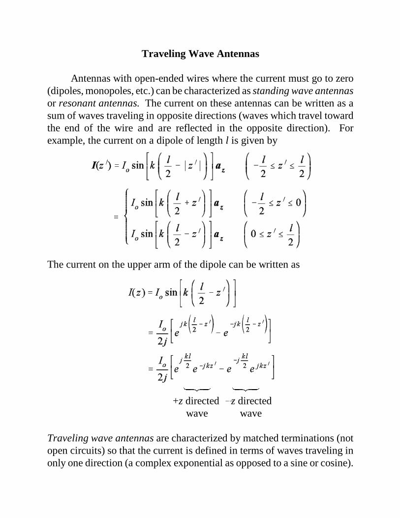
A traveling wave antenna can be formed by a single wire transmission line(single wire over ground) which is terminated with a matched load (noreflection). Typically, the length of the transmission line is severalwavelengths.

The antenna shown above is commonly called a Beverage or waveantenna. This antenna can be analyzed as a rectangular loop, according toimage theory. However, the effects of an imperfect ground may besignificant and can be included using the reflection coefficient approach.The contribution to the far fields due to the vertical conductors is typicallyneglected since it is small if l >> h. Note that the antenna does not radiateefficiently if the height h is small relative to wavelength. In an alternativetechnique of analyzing this antenna, the far field produced by a longisolated wire of length l can be determined and the overall far field foundusing the 2 element array factor.

Traveling wave antennas are commonly formed using wire segmentswith different geometries. Therefore, the antenna far field can be obtainedby superposition using the far fields of the individual segments. Thus, theradiation characteristics of a long straight segment of wire carrying atraveling wave type of current are necessary to analyze the typical travelingwave antenna.

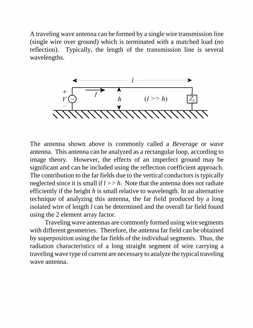
Consider a segment of a traveling wave antenna (an electrically longwire of length l lying along the z-axis) as shown below. A traveling wavecurrent flows in the z-direction.

� - attenuation constant

� - phase constant

If the losses for the antenna are negligible (ohmic loss in the conductors,loss due to imperfect ground, etc.), then the current can be written as

The far field vector potential is

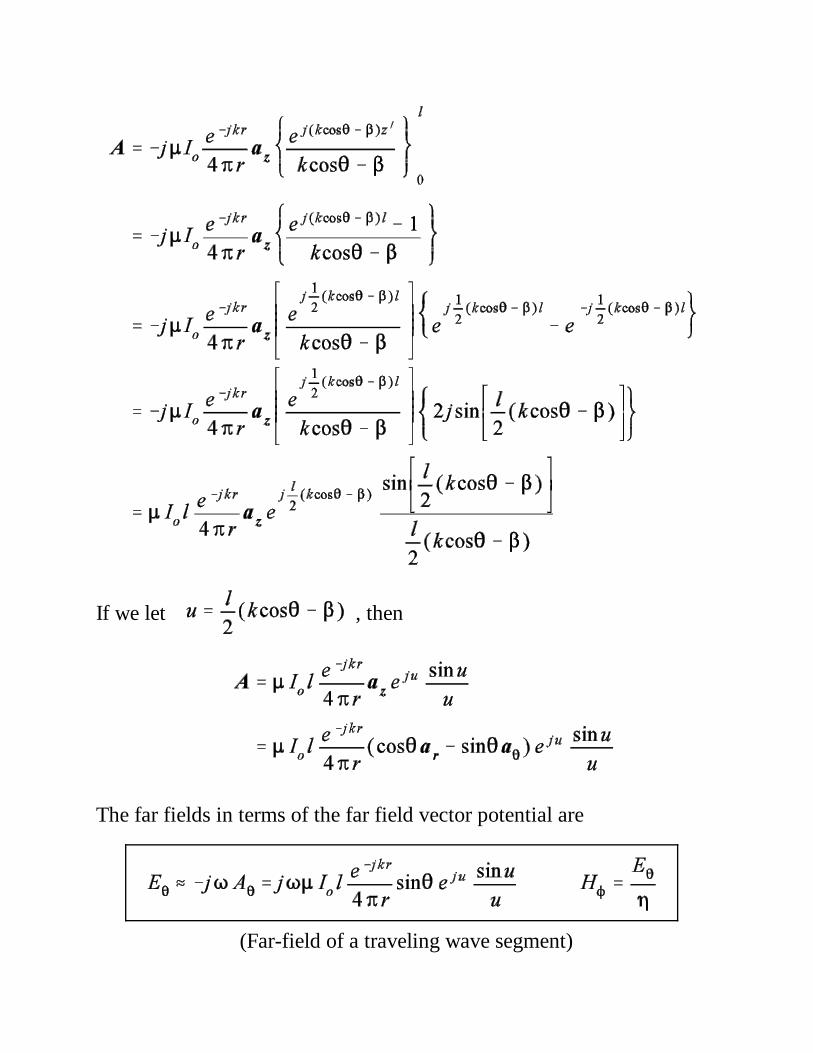
If we let , then

The far fields in terms of the far field vector potential are

(Far-field of a traveling wave segment)

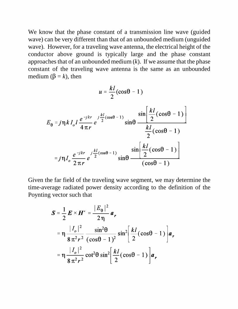
We know that the phase constant of a transmission line wave (guidedwave) can be very different than that of an unbounded medium (unguidedwave). However, for a traveling wave antenna, the electrical height of theconductor above ground is typically large and the phase constantapproaches that of an unbounded medium (k). If we assume that the phaseconstant of the traveling wave antenna is the same as an unboundedmedium (� = k), then

Given the far field of the traveling wave segment, we may determine thetime-average radiated power density according to the definition of thePoynting vector such that

The total power radiated by the traveling wave segment is found byintegrating the Poynting vector.

and the radiation resistance is

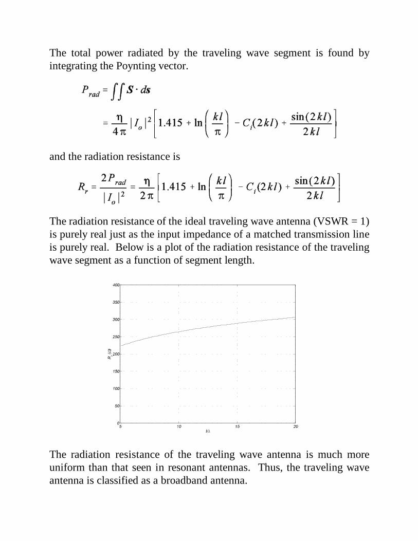
The radiation resistance of the ideal traveling wave antenna (VSWR = 1)is purely real just as the input impedance of a matched transmission lineis purely real. Below is a plot of the radiation resistance of the travelingwave segment as a function of segment length.

The radiation resistance of the traveling wave antenna is much moreuniform than that seen in resonant antennas. Thus, the traveling waveantenna is classified as a broadband antenna.

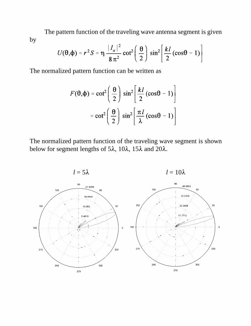
The pattern function of the traveling wave antenna segment is givenby

The normalized pattern function can be written as

The normalized pattern function of the traveling wave segment is shownbelow for segment lengths of 5�, 10�, 15� and 20�.

l = 5� l = 10�

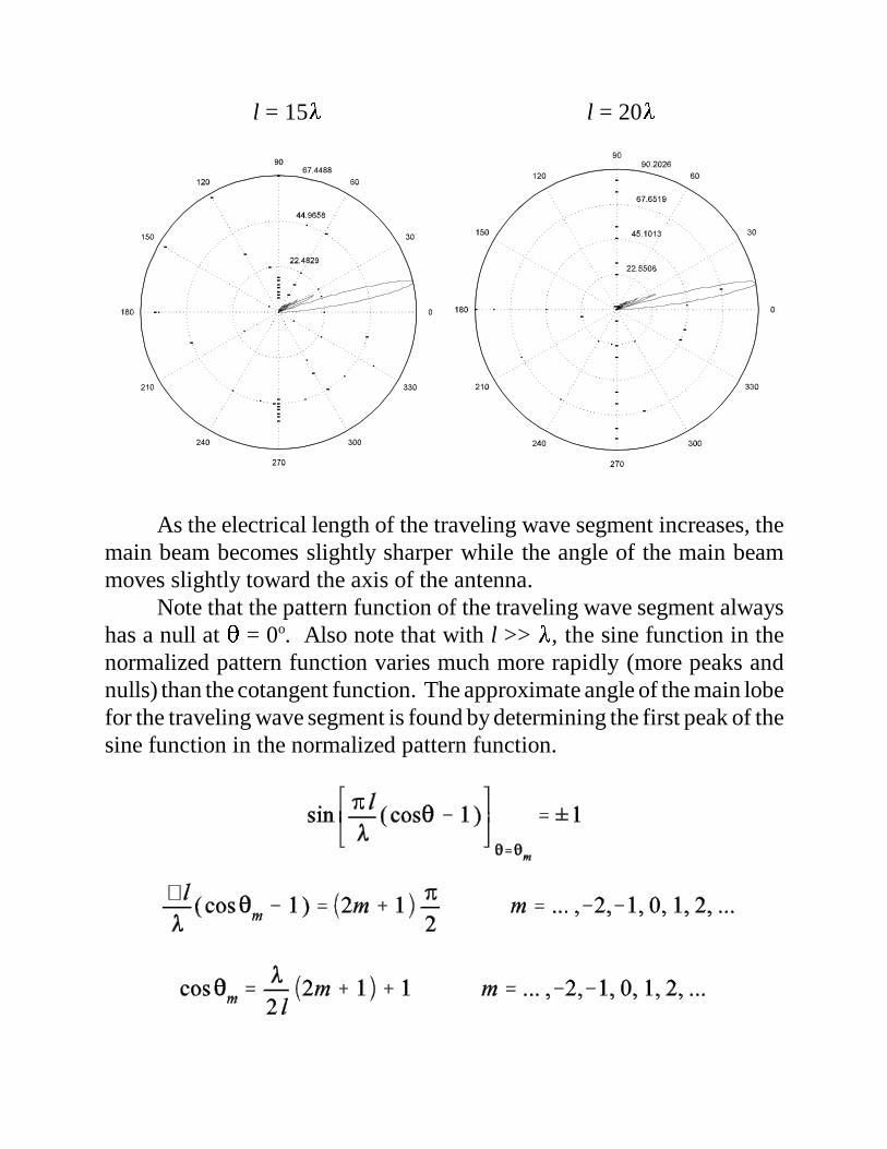
l = 15� l = 20�

As the electrical length of the traveling wave segment increases, themain beam becomes slightly sharper while the angle of the main beammoves slightly toward the axis of the antenna.

Note that the pattern function of the traveling wave segment alwayshas a null at � = 0o. Also note that with l >> �, the sine function in thenormalized pattern function varies much more rapidly (more peaks andnulls) than the cotangent function. The approximate angle of the main lobefor the traveling wave segment is found by determining the first peak of thesine function in the normalized pattern function.

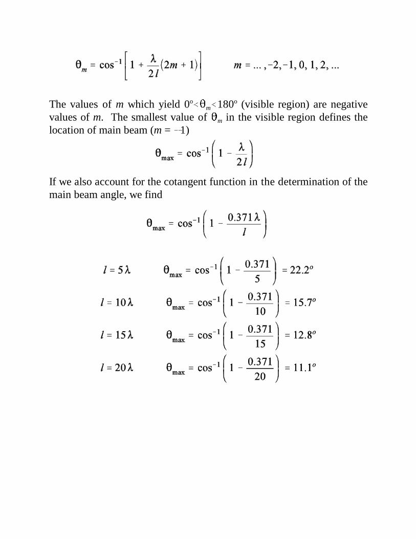
The values of m which yield 0o��m�180o (visible region) are negative

values of m. The smallest value of �m in the visible region defines thelocation of main beam (m = �1)

If we also account for the cotangent function in the determination of themain beam angle, we find

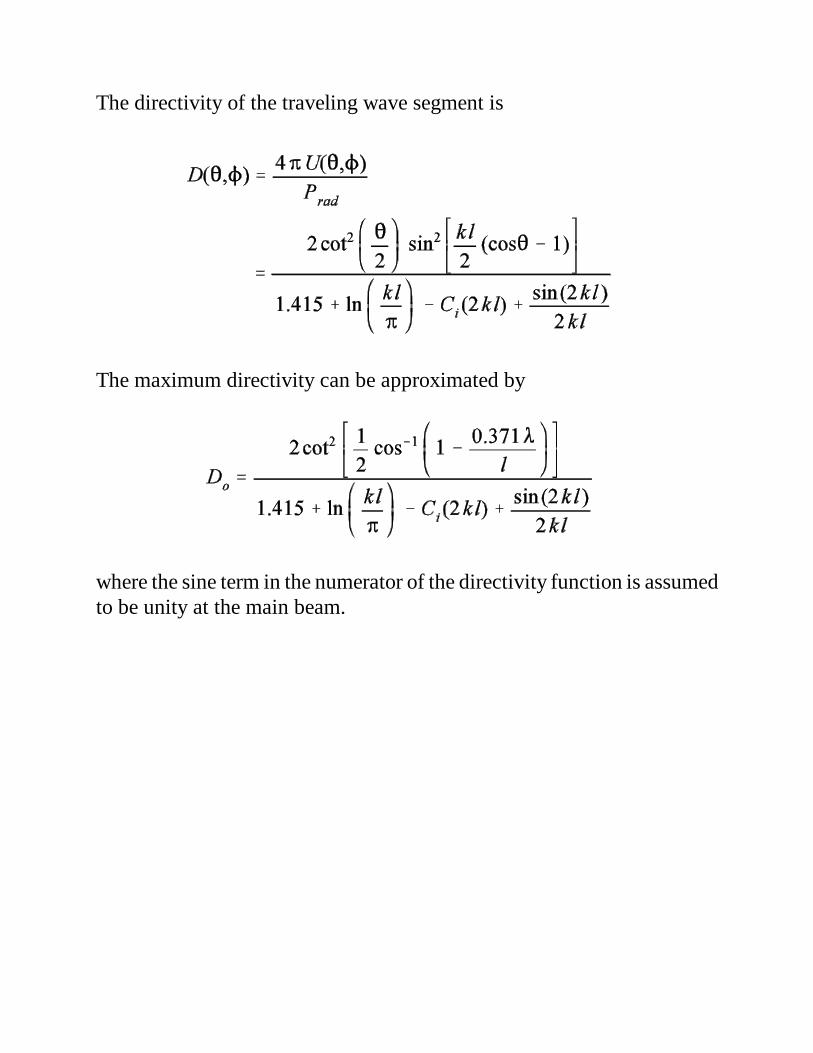
The directivity of the traveling wave segment is

The maximum directivity can be approximated by

where the sine term in the numerator of the directivity function is assumedto be unity at the main beam.

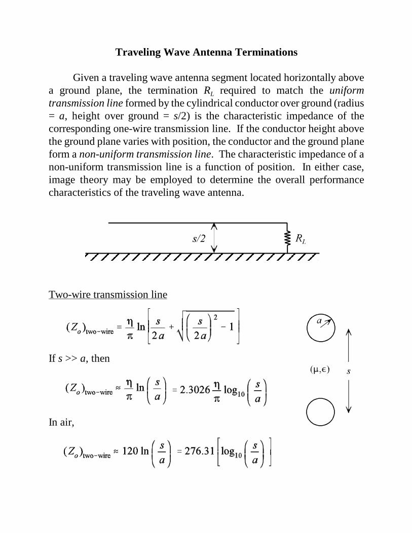
Traveling Wave Antenna Terminations

Given a traveling wave antenna segment located horizontally abovea ground plane, the termination RL required to match the uniformtransmission line formed by the cylindrical conductor over ground (radius= a, height over ground = s/2) is the characteristic impedance of thecorresponding one-wire transmission line. If the conductor height abovethe ground plane varies with position, the conductor and the ground planeform a non-uniform transmission line. The characteristic impedance of anon-uniform transmission line is a function of position. In either case,image theory may be employed to determine the overall performancecharacteristics of the traveling wave antenna.

Two-wire transmission line

If s >> a, then

In air,

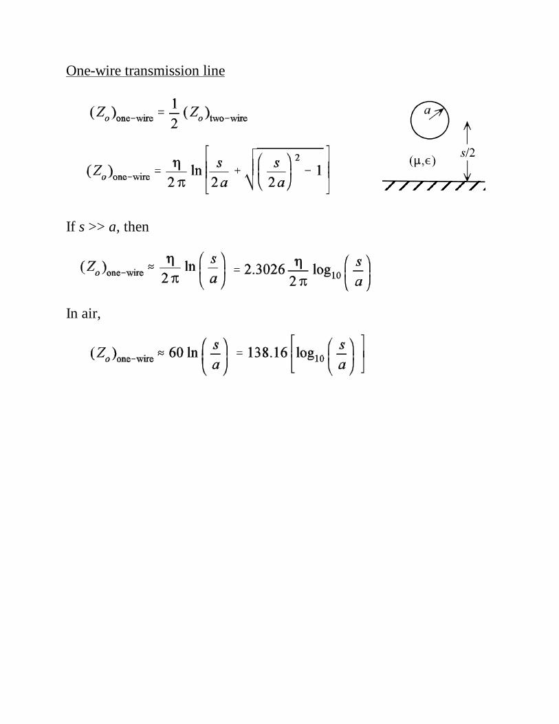
One-wire transmission line

If s >> a, then

In air,

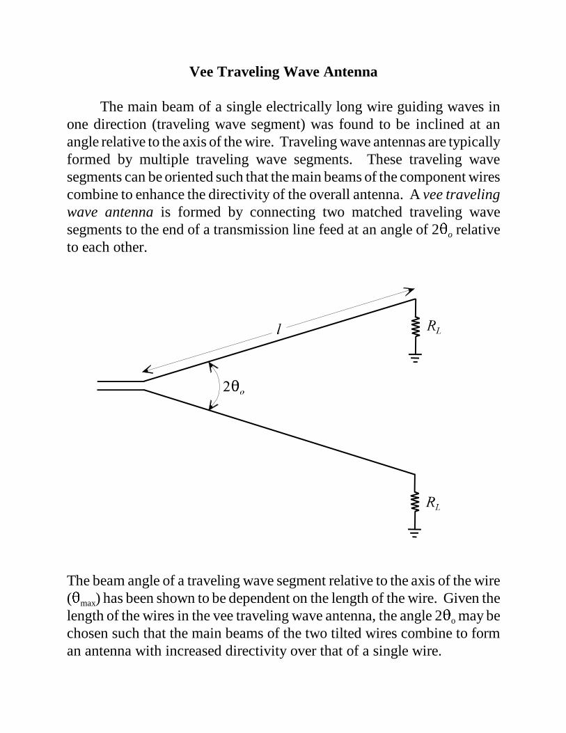
Vee Traveling Wave Antenna

The main beam of a single electrically long wire guiding waves inone direction (traveling wave segment) was found to be inclined at anangle relative to the axis of the wire. Traveling wave antennas are typicallyformed by multiple traveling wave segments. These traveling wavesegments can be oriented such that the main beams of the component wirescombine to enhance the directivity of the overall antenna. A vee travelingwave antenna is formed by connecting two matched traveling wavesegments to the end of a transmission line feed at an angle of 2�o relativeto each other.

The beam angle of a traveling wave segment relative to the axis of the wire(�max) has been shown to be dependent on the length of the wire. Given thelength of the wires in the vee traveling wave antenna, the angle 2�o may bechosen such that the main beams of the two tilted wires combine to forman antenna with increased directivity over that of a single wire.

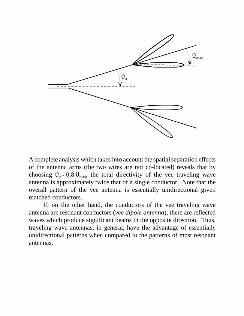
A complete analysis which takes into account the spatial separation effectsof the antenna arms (the two wires are not co-located) reveals that bychoosing �o� 0.8 �max, the total directivity of the vee traveling waveantenna is approximately twice that of a single conductor. Note that theoverall pattern of the vee antenna is essentially unidirectional givenmatched conductors.

If, on the other hand, the conductors of the vee traveling waveantenna are resonant conductors (vee dipole antenna), there are reflectedwaves which produce significant beams in the opposite direction. Thus,traveling wave antennas, in general, have the advantage of essentiallyunidirectional patterns when compared to the patterns of most resonantantennas.

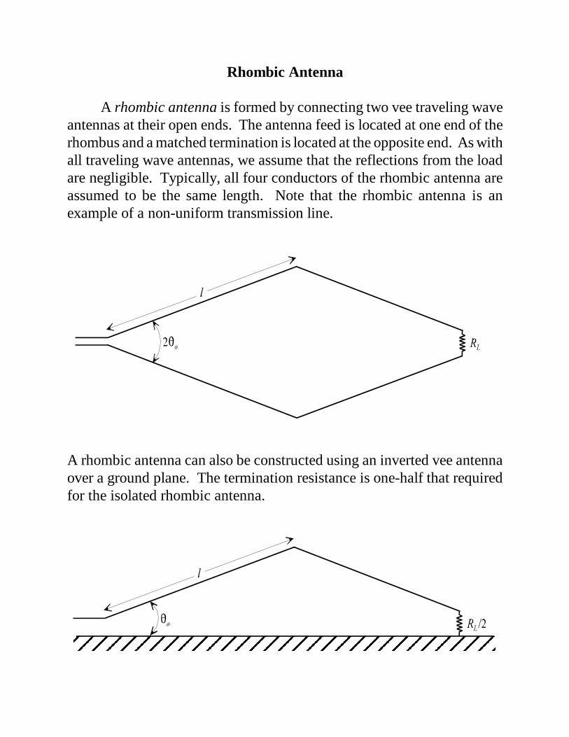
Rhombic Antenna

A rhombic antenna is formed by connecting two vee traveling waveantennas at their open ends. The antenna feed is located at one end of therhombus and a matched termination is located at the opposite end. As withall traveling wave antennas, we assume that the reflections from the loadare negligible. Typically, all four conductors of the rhombic antenna areassumed to be the same length. Note that the rhombic antenna is anexample of a non-uniform transmission line.

A rhombic antenna can also be constructed using an inverted vee antennaover a ground plane. The termination resistance is one-half that requiredfor the isolated rhombic antenna.

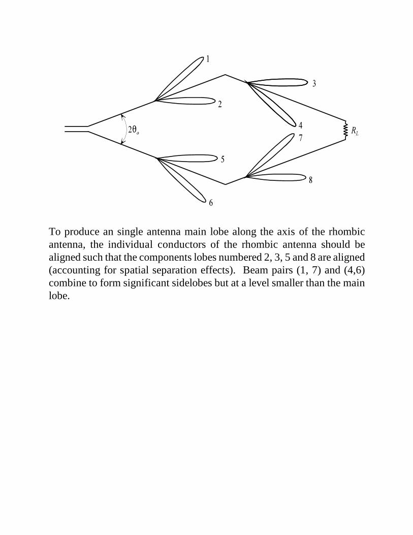
To produce an single antenna main lobe along the axis of the rhombicantenna, the individual conductors of the rhombic antenna should bealigned such that the components lobes numbered 2, 3, 5 and 8 are aligned(accounting for spatial separation effects). Beam pairs (1, 7) and (4,6)combine to form significant sidelobes but at a level smaller than the mainlobe.

Yagi-Uda Array

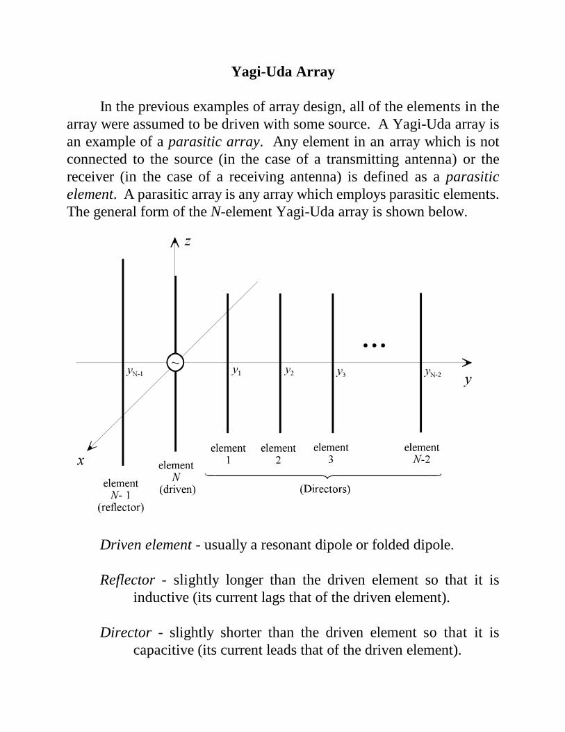
In the previous examples of array design, all of the elements in thearray were assumed to be driven with some source. A Yagi-Uda array isan example of a parasitic array. Any element in an array which is notconnected to the source (in the case of a transmitting antenna) or thereceiver (in the case of a receiving antenna) is defined as a parasiticelement. A parasitic array is any array which employs parasitic elements.The general form of the N-element Yagi-Uda array is shown below.

Driven element - usually a resonant dipole or folded dipole.

Reflector - slightly longer than the driven element so that it isinductive (its current lags that of the driven element).

Director - slightly shorter than the driven element so that it iscapacitive (its current leads that of the driven element).

Yagi-Uda Array Advantages

� Lightweight� Low cost� Simple construction� Unidirectional beam (front-to-back ratio)� Increased directivity over other simple wire antennas� Practical for use at HF (3-30 MHz), VHF (30-300 MHz), and

UHF (300 MHz - 3 GHz)

Typical Yagi-Uda Array Parameters

Driven element � half-wave resonant dipole or folded dipole,(Length = 0.45� to 0.49�, dependent on radius), folded dipolesare employed as driven elements to increase the array inputimpedance.

Director � Length = 0.4� to 0.45� (approximately 10 to 20 % shorterthan the driven element), not necessarily uniform.

Reflector � Length � 0.5� (approximately 5 to 10 % longer than thedriven element).

Director spacing � approximately 0.2 to 0.4�, not necessarilyuniform.

Reflector spacing � 0.1 to 0.25�

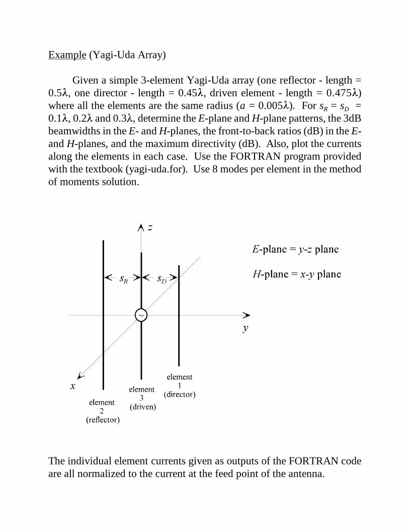
Example (Yagi-Uda Array)

Given a simple 3-element Yagi-Uda array (one reflector - length =0.5�, one director - length = 0.45�, driven element - length = 0.475�)where all the elements are the same radius (a = 0.005�). For sR = sD =0.1�, 0.2� and 0.3�, determine the E-plane and H-plane patterns, the 3dBbeamwidths in the E- and H-planes, the front-to-back ratios (dB) in the E-and H-planes, and the maximum directivity (dB). Also, plot the currentsalong the elements in each case. Use the FORTRAN program providedwith the textbook (yagi-uda.for). Use 8 modes per element in the methodof moments solution.

The individual element currents given as outputs of the FORTRAN codeare all normalized to the current at the feed point of the antenna.

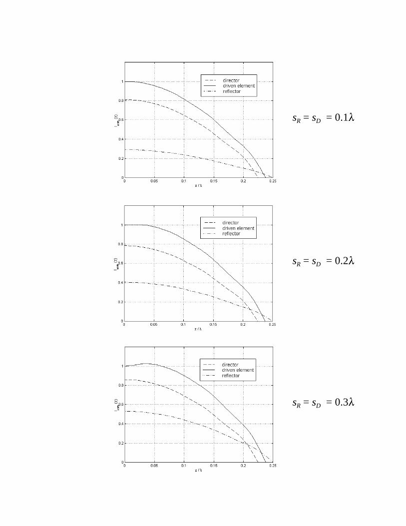
sR = sD = 0.1�

sR = sD = 0.2�

sR = sD = 0.3�

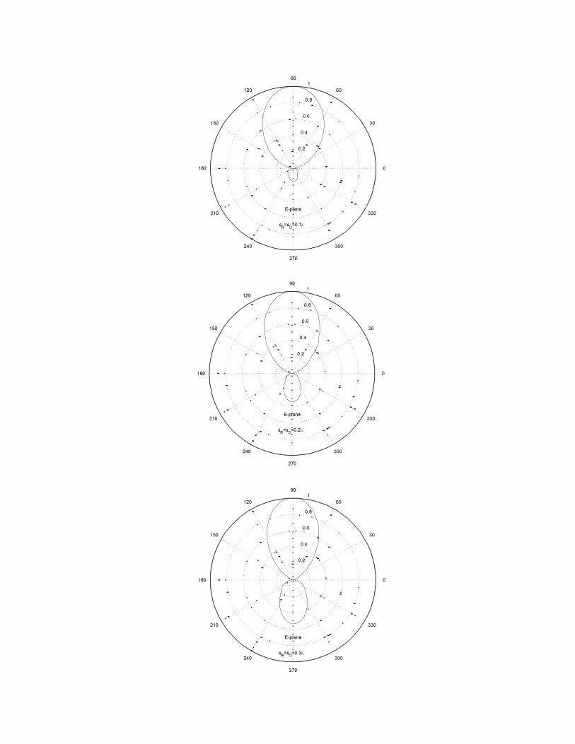
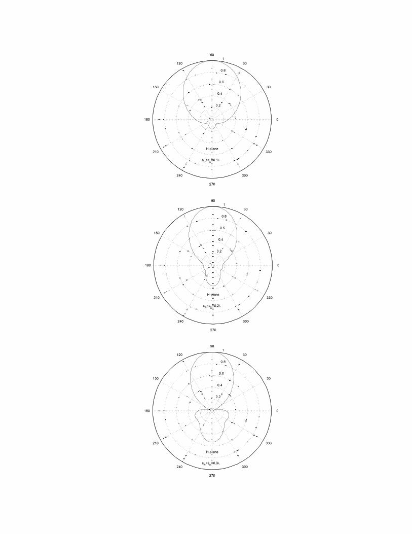
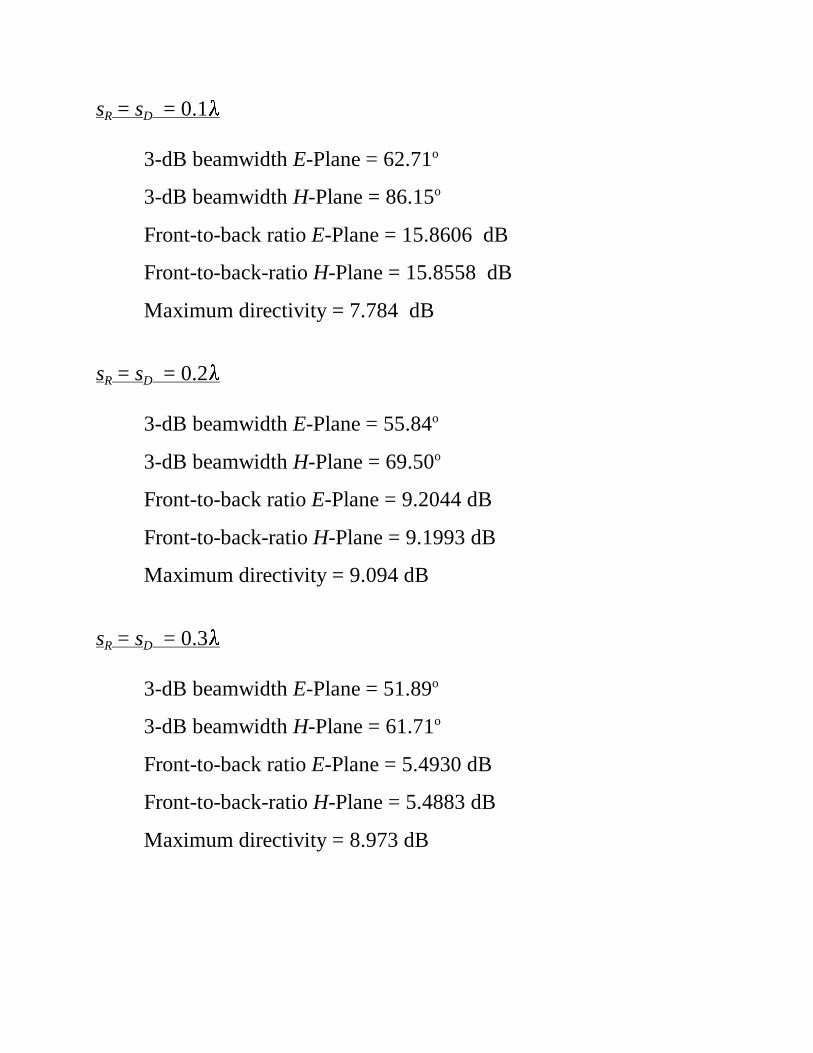
sR = sD = 0.1�

3-dB beamwidth E-Plane = 62.71o

3-dB beamwidth H-Plane = 86.15o

Front-to-back ratio E-Plane = 15.8606 dB

Front-to-back-ratio H-Plane = 15.8558 dB

Maximum directivity = 7.784 dB

sR = sD = 0.2�

3-dB beamwidth E-Plane = 55.84o

3-dB beamwidth H-Plane = 69.50o

Front-to-back ratio E-Plane = 9.2044 dB

Front-to-back-ratio H-Plane = 9.1993 dB

Maximum directivity = 9.094 dB

sR = sD = 0.3�

3-dB beamwidth E-Plane = 51.89o

3-dB beamwidth H-Plane = 61.71o

Front-to-back ratio E-Plane = 5.4930 dB

Front-to-back-ratio H-Plane = 5.4883 dB

Maximum directivity = 8.973 dB

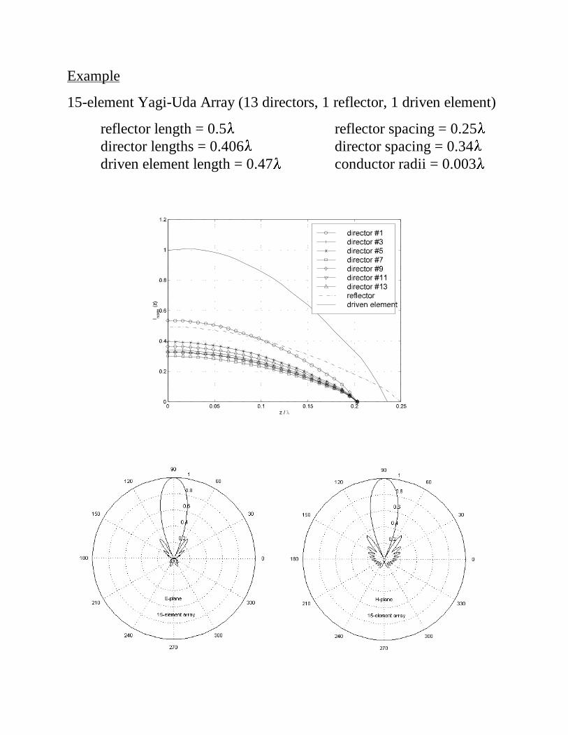
Example

15-element Yagi-Uda Array (13 directors, 1 reflector, 1 driven element)

reflector length = 0.5� reflector spacing = 0.25�director lengths = 0.406� director spacing = 0.34�driven element length = 0.47� conductor radii = 0.003�

3-dB beamwidth E-Plane = 26.79o

3-dB beamwidth H-Plane = 27.74o

Front-to-back ratio E-Plane = 36.4422 dB

Front-to-back-ratio H-Plane = 36.3741 dB

Maximum directivity = 14.700 dB

(1)

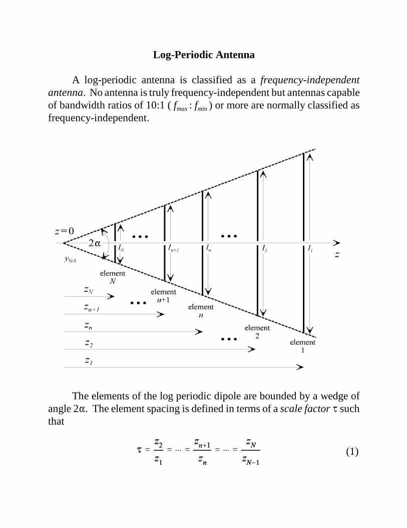
Log-Periodic Antenna

A log-periodic antenna is classified as a frequency-independentantenna. No antenna is truly frequency-independent but antennas capableof bandwidth ratios of 10:1 ( fmax : fmin ) or more are normally classified asfrequency-independent.

The elements of the log periodic dipole are bounded by a wedge ofangle 2�. The element spacing is defined in terms of a scale factor � suchthat

(2)

(3)

(4)

(5)

(6)

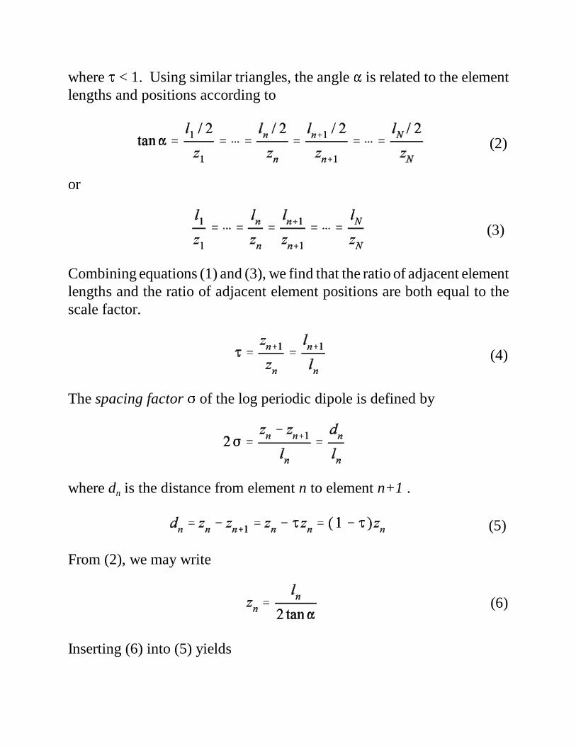
where � < 1. Using similar triangles, the angle � is related to the elementlengths and positions according to

or

Combining equations (1) and (3), we find that the ratio of adjacent elementlengths and the ratio of adjacent element positions are both equal to thescale factor.

The spacing factor � of the log periodic dipole is defined by

where dn is the distance from element n to element n+1 .

From (2), we may write

Inserting (6) into (5) yields

(7)

(8)

(9)

(10)

(11)

Combining equation (3) with equation (7) gives

or

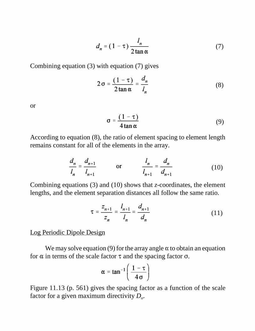
According to equation (8), the ratio of element spacing to element lengthremains constant for all of the elements in the array.

Combining equations (3) and (10) shows that z-coordinates, the elementlengths, and the element separation distances all follow the same ratio.

Log Periodic Dipole Design

We may solve equation (9) for the array angle � to obtain an equationfor � in terms of the scale factor � and the spacing factor �.

Figure 11.13 (p. 561) gives the spacing factor as a function of the scalefactor for a given maximum directivity Do.

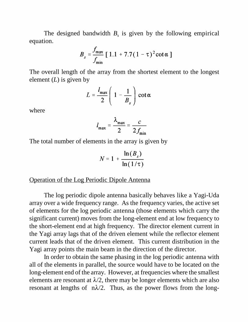
The designed bandwidth Bs is given by the following empiricalequation.

The overall length of the array from the shortest element to the longestelement (L) is given by

where

The total number of elements in the array is given by

Operation of the Log Periodic Dipole Antenna

The log periodic dipole antenna basically behaves like a Yagi-Udaarray over a wide frequency range. As the frequency varies, the active setof elements for the log periodic antenna (those elements which carry thesignificant current) moves from the long-element end at low frequency tothe short-element end at high frequency. The director element current inthe Yagi array lags that of the driven element while the reflector elementcurrent leads that of the driven element. This current distribution in theYagi array points the main beam in the direction of the director.

In order to obtain the same phasing in the log periodic antenna withall of the elements in parallel, the source would have to be located on thelong-element end of the array. However, at frequencies where the smallestelements are resonant at �/2, there may be longer elements which are alsoresonant at lengths of n�/2. Thus, as the power flows from the long-

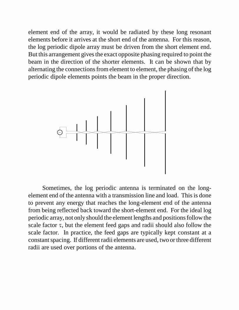
element end of the array, it would be radiated by these long resonantelements before it arrives at the short end of the antenna. For this reason,the log periodic dipole array must be driven from the short element end.But this arrangement gives the exact opposite phasing required to point thebeam in the direction of the shorter elements. It can be shown that byalternating the connections from element to element, the phasing of the logperiodic dipole elements points the beam in the proper direction.

Sometimes, the log periodic antenna is terminated on the long-element end of the antenna with a transmission line and load. This is doneto prevent any energy that reaches the long-element end of the antennafrom being reflected back toward the short-element end. For the ideal logperiodic array, not only should the element lengths and positions follow thescale factor �, but the element feed gaps and radii should also follow thescale factor. In practice, the feed gaps are typically kept constant at aconstant spacing. If different radii elements are used, two or three differentradii are used over portions of the antenna.

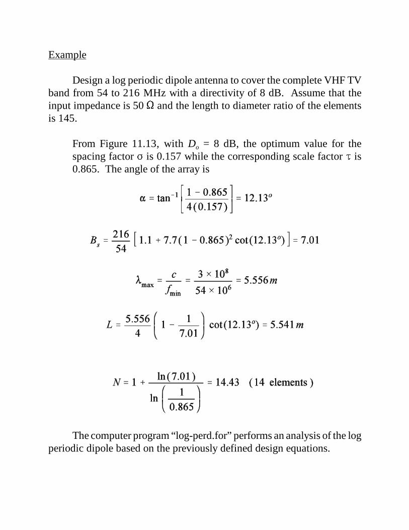
Example

Design a log periodic dipole antenna to cover the complete VHF TVband from 54 to 216 MHz with a directivity of 8 dB. Assume that theinput impedance is 50 � and the length to diameter ratio of the elementsis 145.

From Figure 11.13, with Do = 8 dB, the optimum value for thespacing factor � is 0.157 while the corresponding scale factor � is0.865. The angle of the array is

The computer program “log-perd.for” performs an analysis of the logperiodic dipole based on the previously defined design equations.

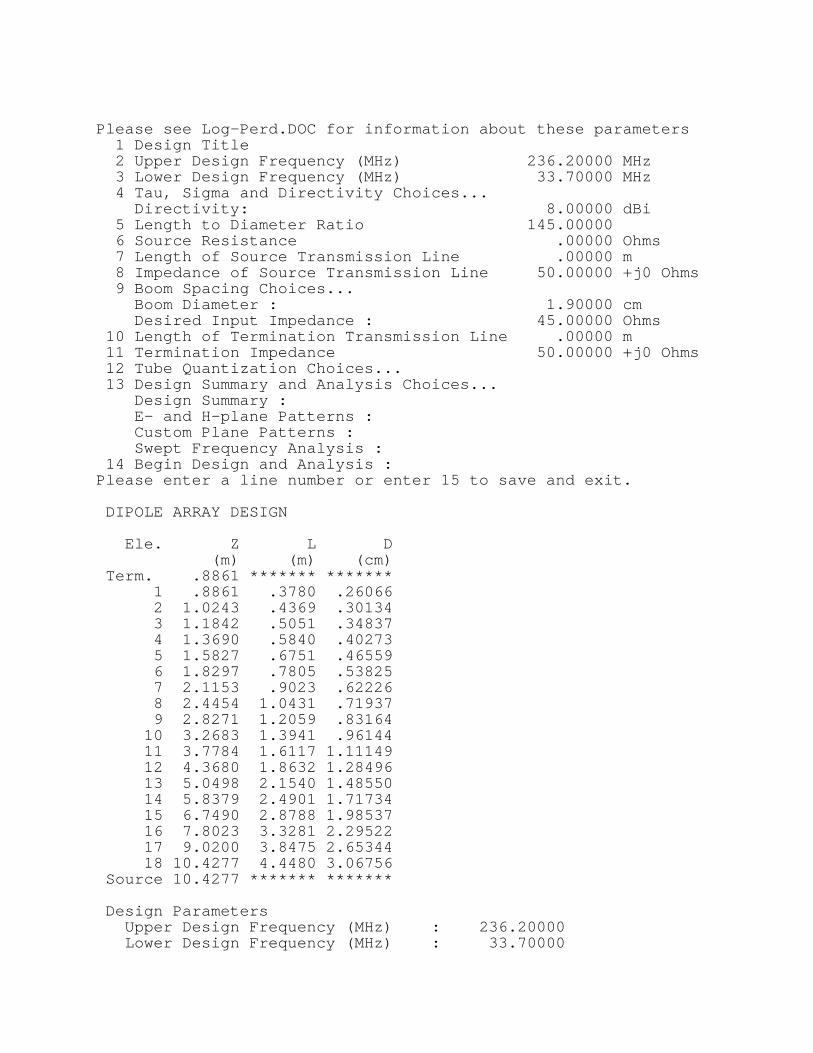
Please see Log-Perd.DOC for information about these parameters 1 Design Title 2 Upper Design Frequency (MHz) 236.20000 MHz 3 Lower Design Frequency (MHz) 33.70000 MHz 4 Tau, Sigma and Directivity Choices... Directivity: 8.00000 dBi 5 Length to Diameter Ratio 145.00000 6 Source Resistance .00000 Ohms 7 Length of Source Transmission Line .00000 m 8 Impedance of Source Transmission Line 50.00000 +j0 Ohms 9 Boom Spacing Choices... Boom Diameter : 1.90000 cm Desired Input Impedance : 45.00000 Ohms 10 Length of Termination Transmission Line .00000 m 11 Termination Impedance 50.00000 +j0 Ohms 12 Tube Quantization Choices... 13 Design Summary and Analysis Choices... Design Summary : E- and H-plane Patterns : Custom Plane Patterns : Swept Frequency Analysis : 14 Begin Design and Analysis :Please enter a line number or enter 15 to save and exit.

DIPOLE ARRAY DESIGN Ele. Z L D (m) (m) (cm) Term. .8861 ******* ******* 1 .8861 .3780 .26066 2 1.0243 .4369 .30134 3 1.1842 .5051 .34837 4 1.3690 .5840 .40273 5 1.5827 .6751 .46559 6 1.8297 .7805 .53825 7 2.1153 .9023 .62226 8 2.4454 1.0431 .71937 9 2.8271 1.2059 .83164 10 3.2683 1.3941 .96144 11 3.7784 1.6117 1.11149 12 4.3680 1.8632 1.28496 13 5.0498 2.1540 1.48550 14 5.8379 2.4901 1.71734 15 6.7490 2.8788 1.98537 16 7.8023 3.3281 2.29522 17 9.0200 3.8475 2.65344 18 10.4277 4.4480 3.06756 Source 10.4277 ******* ******* Design Parameters Upper Design Frequency (MHz) : 236.20000 Lower Design Frequency (MHz) : 33.70000

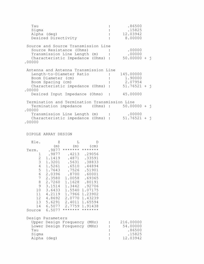
Tau : .86500 Sigma : .15825 Alpha (deg) : 12.03942 Desired Directivity : 8.00000 Source and Source Transmission Line Source Resistance (Ohms) : .00000 Transmission Line Length (m) : .00000 Characteristic Impedance (Ohms) : 50.00000 + j .00000 Antenna and Antenna Transmission Line Length-to-Diameter Ratio : 145.00000 Boom Diameter (cm) : 1.90000 Boom Spacing (cm) : 2.07954 Characteristic impedance (Ohms) : 51.76521 + j .00000 Desired Input Impedance (Ohms) : 45.00000 Termination and Termination Transmission Line Termination impedance (Ohms) : 50.00000 + j .00000 Transmission Line Length (m) : .00000 Characteristic impedance (Ohms) : 51.76521 + j .00000

DIPOLE ARRAY DESIGN Ele. Z L D (m) (m) (cm) Term. .9877 ******* ******* 1 .9877 .4213 .29056 2 1.1419 .4871 .33591 3 1.3201 .5631 .38833 4 1.5261 .6510 .44894 5 1.7643 .7526 .51901 6 2.0396 .8700 .60001 7 2.3580 1.0058 .69365 8 2.7260 1.1628 .80191 9 3.1514 1.3442 .92706 10 3.6433 1.5540 1.07175 11 4.2119 1.7966 1.23902 12 4.8692 2.0770 1.43239 13 5.6291 2.4011 1.65594 14 6.5077 2.7759 1.91438 Source 6.5077 ******* ******* Design Parameters Upper Design Frequency (MHz) : 216.00000 Lower Design Frequency (MHz) : 54.00000 Tau : .86500 Sigma : .15825 Alpha (deg) : 12.03942

1

2

3

4

5

30

210

60

240

90

270

120

300

150

330

180 0

E-Plane, f = 54 MHz

1

2

3

4

5

30

210

60

240

90

270

120

300

150

330

180 0

H-Plane, f = 54 MHz

Desired Directivity : 8.00000 Source and Source Transmission Line Source Resistance (Ohms) : .00000 Transmission Line Length (m) : .00000 Characteristic Impedance (Ohms) : 50.00000 + j .00000 Antenna and Antenna Transmission Line Length-to-Diameter Ratio : 145.00000 Boom Diameter (cm) : 1.90000 Boom Spacing (cm) : 2.07954 Characteristic impedance (Ohms) : 51.76521 + j .00000 Desired Input Impedance (Ohms) : 45.00000 Termination and Termination Transmission Line Termination impedance (Ohms) : 50.00000 + j .00000 Transmission Line Length (m) : .00000 Characteristic impedance (Ohms) : 51.76521 + j .00000

2

4

6

8

30

210

60

240

90

270

120

300

150

330

180 0

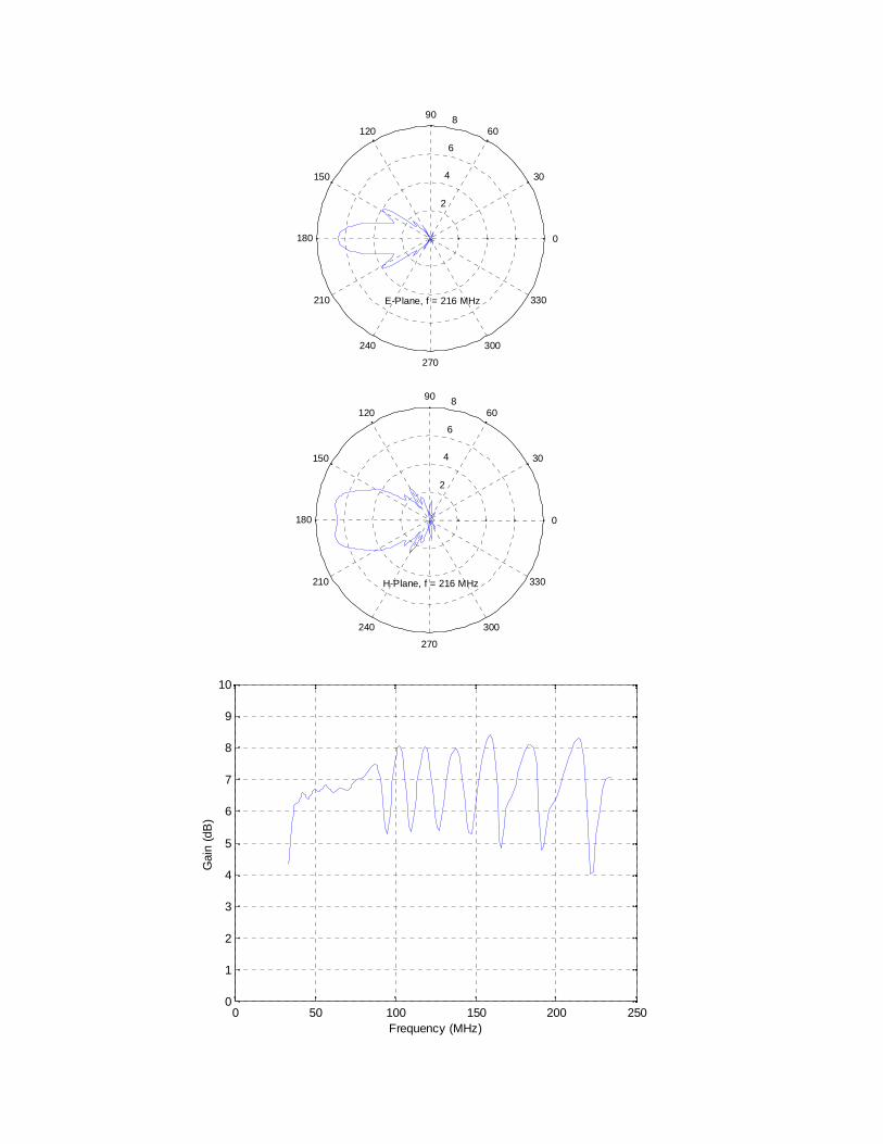
E-Plane, f = 216 MHz

2

4

6

8

30

210

60

240

90

270

120

300

150

330

180 0

H-Plane, f = 216 MHz

0 50 100 150 200 2500

1

2

3

4

5

6

7

8

9

10

Frequency (MHz)

Gai

n (d

B)