Lat. Am. J. Phys. Educ. Vol 5, No. 1, March 2011 5 http://www.lajpe.org

Traveling along a zipline

Carl E. Mungan1 and Trevor C. Lipscombe2 1Physics Department, U.S. Naval Academy, Annapolis, Maryland, 21402-1363, USA. 2Catholic University of America Press, Washington, DC, 20064, USA. E-mail: mungan@usna.edu (Received 19 November 2010; accepted 31 January 2011)

Abstract The trajectory of a rider slowly traversing a zipline of fixed length and endpoints is computed, as a one-dimensional illustration of the curving of spacetime by a mass. As the rider’s weight increases from 0 to ∞, the trajectories uniformly interpolate between a catenary and an ellipse. These results are obtained by balancing forces in the horizontal and vertical directions, so that the treatment is accessible to undergraduate physics majors who have been exposed to finding the numerical roots of an algebraic equation. Keywords: Zipline, curved spacetime, force balance, catenary.

Resumen La trayectoria de un jinete lentamente atravesando una tirolesa de longitud fija y criterios de valoración se calcula, como una ilustración de una dimensión de la curvatura del espacio-tiempo por una masa. A medida que aumenta el peso del ciclista de 0 a, las trayectorias de manera uniforme interpolar entre una catenaria y una elipse. Estos resultados se obtienen al equilibrar las fuerzas en las direcciones horizontal y vertical, de modo que el tratamiento es accesible para mayores de física de pregrado que han estado expuestos a la búsqueda de las raíces numérica de una ecuación algebraica. Palabras clave: Tirolesa, espacio-tiempo curvado, balance de la fuerza, la catenaria. PACS: 45.20.D–, 46.05.+b, 02.40.-k ISSN 1870-9095

I. INTRODUCTION Consider a uniform-density cable of total mass m and length L. (Nonuniform cables can also be treated [1–2].) Suppose one end is fixed at the origin of a coordinate system with the x axis pointing rightward toward the other fixed end that is assumed to be lower (or equal) in height than it. Defining the y axis to point downward, this second end is thus at position

( X ,Y ) where X > 0 and Y ! 0 such that the cable is not taut (i.e., L

2> X

2+ Y

2 ). The cable freely hangs in a uniform gravitational field g. A person of mass M now clips onto the cable near the origin and pulls himself along the resulting zipline to the far end. The problem consists in finding the path of the person’s center of mass as he traverses the line, as a way of introducing the idea of curved space in general relativity [3–4]. That is to say, the particle (rider) is moving in a curved space (the zipline) but the curvature of the space is distorted by the position of the particle, thereby illustrating John Wheeler’s maxim that “spacetime tells matter how to move, while the moving matter tells spacetime how to curve” and providing a one-dimensional (1D) analogy [5] to the 2D illustration of a heavy marble rolling around on a stretched rubber sheet [6]. A 1D model has the advantage that it is relatively straightforward to calculate and plot.

The article is organized as follows. First, a relation is found between the tension in the cable at any point along the

line and the angle the cable makes with the horizontal at that same point. Next, the coordinates of the rider (relative to the left-hand end of the cable) are expressed in terms of his fractional distance along the cable and two dimensionless parameters characterizing the zipline. By letting that fractional distance equal unity, the coordinates of the right-hand end of the cable are found. Finally, by similarly calculating the coordinates of the rider relative to the right-hand end of the cable, the rider’s trajectory is numerically computed (using a root-finding algorithm) by matching the coordinates determined relative to the two ends of the cable. The last section of the paper establishes the limiting cases wherein the trajectory becomes hyperbolic (i.e., the familiar catenary solution) in the limit of a low-weight rider (relative to the cable’s weight) and elliptical in the opposite limit of a heavy rider. II. CALCULATING THE TRAJECTORY OF THE RIDER Consider the situation when the rider is located at position

(xr , yr ) , a fraction f of the distance along the cable’s length. The cable bows downward in smooth curves to the left and right of the person, but there will be a cusp in the zipline at the person’s position [7], as illustrated in Fig. 1. At any point

(x, y) along the cable, the line to the right of that point

Carl E. Mungan and Trevor C. Lipscombe

Lat. Am. J. Phys. Educ. Vol 5, No. 1, March 2011 6 http://www.lajpe.org

makes angle θ relative to the +x axis. In particular, the zipline makes angle

!

0 at the end attached to the origin.

FIGURE 1. Geometry of the zipline indicating the coordinates of the two endpoints at

(0,0) and

( X ,Y ) , of the rider of mass M at

(x

r, y

r) , and of arbitrary points

(x, y) and

( !x , !y ) along the line

to the left and right of the rider, respectively. The particular case plotted here is for parameters

!

i= 45° and

!

f= "10° (before the

rider mounts the line), ! = 1 (i.e., the rider has the same total mass

as the zipline), L = 1 (i.e., the zipline has unit length), and

f = 0.25 (i.e, the rider is located a quarter of the way along the length of the cable). As explained in Sec. III, the zipline has the shape of one catenary between points

(0,0) and

(x

r, y

r) , and

another catenary between (x

r, y

r) and

( X ,Y ) .

Now consider the segment of the cable extending from the origin to the point

(x, y) a distance ! along it. (Assume

! < f L so that the segment does not include the rider.) There are three forces on this segment: the tensions

T

0 and T

at its two ends, pulling tangential to the line (i.e., at angles

!

0 and θ), and the segment’s weight

mg ! / L . The line is

always in equilibrium, assuming the rider traverses it slowly.1 In that case, the three forces must balance. For their x components, that implies

T

0cos!

0= T cos!. (1)

Therefore the product of the tension and the cosine of the angle has some constant value K along the cable. To rewrite it as a dimensionless constant, define

b ! mg / K , so that

T cos! = mg / b. (2)

Similarly, balancing the y components of the forces on the segment implies

T

0sin!

0= T sin! + mg

!

L. (3)

1Here “slowly” means the rider’s acceleration is negligible and his speed υ is always much less than the speed of even the slowest transverse waves on the zipline, i.e., min /T L m! << where

minT is the tension in the cable at

the point where it makes the smallest angle θ relative to the horizontal, according to Eq. (1). This idea of slowness is analogous to the requirement that the speed of a piston in a gas-filled cylinder must always be much less than the speed of sound of the gas if the compressions are to be considered quasistatic.

Next, divide Eq. (3) by (2)—or alternatively by Eq. (1)—to eliminate the tensions and obtain

tan!0= tan! + b

!

L. (4)

Defining another dimensionless constant

a ! tan"

0 and a

dimensionless variable u ! ! / L , Eq. (4) becomes

tan! = a " bu. (5)

The coordinates of the rider can be found by dividing the cable to the left of him into differential pieces of length d! . Integrating the x-components of the length of each piece gives

xr= dl cos!

0

f L

" . (6)

Divide both sides of this equation by the total length L of the cable to obtain the normalized x-coordinate of the rider as

!x = du cos!0

f

" . (7)

Substituting Eq. (5) into the identity

cos! = 1 / sec! = (1+ tan2

! )"1/2 , the integral in Eq. (7) can be performed to obtain the natural logarithm

!x =1

bln

a + 1+ a2

a ! bf + 1+ (a ! bf )2

"

#

$$

%

&

''. (8)

If there is no rider on the zipline, then this relation is valid along its entire length, in which case

f = 1 . Then defining

!X ! X / L , Eq. (8) becomes

!X =1

b0

lna0 + 1+ a0

2

a0 ! b0 + 1+ (a0 ! b0 )2

"

#

$$$

%

&

'''

, (9)

where zero subscripts were added to the two constants a and b to indicate that these are their values when the rider has zero mass. Similarly, the normalized y-coordinate of the rider,

!y , can be obtained by replacing cos! with

sin! = (1" cos2

! )1/2 in Eq. (7), and the resulting integral this time gives

!y =

1+ a2! 1+ (a ! bf )2

b. (10)

Again, with no rider on the line, put

f = 1 and

!Y ! Y / L to

obtain

Traveling along a zipline

Lat. Am. J. Phys. Educ. Vol 5, No. 1, March 2011 7 http://www.lajpe.org

!Y =

1+ a02! 1+ (a0 ! b0 )2

b0

. (11)

Equations (9) and (11) cannot be analytically inverted to find

a

0 and

b0

in terms of !X and !Y . So rather than spelling out the solution to the problem in terms of the position

( X ,Y ) of

the right-hand end of the cable, it makes more sense to write it in terms of the angles

!

i and

!

f that the cable makes at its

two ends without a rider.2 Recalling the definition of a and solving Eq. (4) for b, one can write

a

0= tan!

i and

b0= tan!

i" tan!

f. (12)

Then the (normalized) position of the right end of the cable can be determined from Eqs. (9) and (11). That position remains fixed as the rider mounts the cable, as does the length of the cable. But the values of a and b change and are no longer equal to

a

0 and

b0

, because the shape (and hence the two end angles) of the cable change with a rider present. In fact, it is clear that even for a fixed (nonzero) rider mass, the values of these two parameters vary as the person changes position f along the zipline. So the problem now becomes one of finding the values of a and b for a given rider position f and mass M (expressed in normalized form as

! " M / m relative to the cable’s mass). The key to solving this problem is that Eqs. (8) and (10) give the position

( !x, !y)

of the cable at the rider’s position relative to the left-hand end of the cable (in terms of the unknowns a and b). Similar equations (in terms of the same two unknowns) give the position

( !!x , ! !y ) of the right-hand end of the cable relative to

the rider.3 By imposing the constraints !x + !!x = !X and

!y + ! !y = !Y , two equations are obtained in the two unknowns

and a root-finding algorithm can be used to solve for a and b. The first step is to find the angle

!"0

of the cable immediately to the right of the rider. For this purpose, consider a segment of the cable that starts at the origin and just barely extends beyond the rider’s point of attachment. Equation (3) can be modified in this case by adding the rider’s weight

Mg to the right-hand side,

T

0sin!

0= "T

0sin "!

0+ mgf + Mg, (13)

where ! became the rider’s position

f L , angle θ became

!"0

, and likewise for the tension T. Again divide this equation by Eq. (2) to get

tan!

0= tan "!

0+ bf + b# . (14)

Consequently the parameter corresponding to a for the right-

2Note that the angle θ anywhere along the cable (including its two ends), with or without a (finite-mass) rider, is limited to the range 90 90!" ° < < + ° since the line can never become vertical according to Eq. (2). Within that range, tan! is always finite and is a single-valued function of θ. 3Hereafter, primes are consistently used to indicate parameters of the cable segment to the right of the rider that correspond to the unprimed parameters of the cable segment to his left.

hand segment of the cable is

!a = a " bf " b# . (15)

Unlike Eq. (3), however, Eq. (1) remains valid even when the point

(x, y) in Fig. 1 is moved to the right of the rider,

because the rider’s gravitational force does not have an x component. Thus K has the same value on the left-hand and right-hand segments of the zipline. Therefore the parameter corresponding to b for the right-hand segment is unchanged, !b = b . Finally, the sum of the lengths of the left-hand and right-hand segments of the cable must be L, and thus the parameter corresponding to f for the right-hand segment must be

!f = 1" f . Now simply substitute these values of

!a , !b , and !f in place of a, b, and f in Eqs. (8) and (10) to

get

!!x =1

bln

a " bf " b# + 1+ (a " bf " b# )2

a " b# " b + 1+ (a " b# " b)2

$

%

&&

'

(

))

, (16)

and

!!y =

1+ (a " bf " b# )2 " 1+ (a " b# " b)2

b. (17)

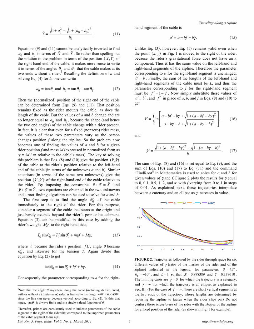
The sum of Eqs. (8) and (16) is set equal to Eq. (9), and the sum of Eqs. (10) and (17) to Eq. (11) and the command “FindRoot” in Mathematica is used to solve for a and b for given values of γ and f. Figure 2 plots the results for γ equal to 0, 0.1, 0.5, 1, 2, and ∞ with f varying from 0 to 1 in steps of 0.01. As explained next, these trajectories interpolate between a catenary and an ellipse as γ increases in value.

FIGURE 2. Trajectories followed by the rider through space for six different values of γ (ratio of the masses of the rider and of the zipline) indicated in the legend, for parameters

!

i= 45° ,

!

f= "10° , and L = 1 so that

X = 0.898389 and Y = 0.339010 .

The limiting cases are ! = 0 for which the trajectory is a catenary,

and ! = " for which the trajectory is an ellipse, as explained in Sec. III. (For the case of ! = " , there are short vertical segments at the two ends of the trajectory, whose lengths are determined by requiring the zipline to tauten when the rider clips on.) Do not confuse these trajectories of the rider with the shapes of the zipline for a fixed position of the rider (as shown in Fig. 1 for example).

Carl E. Mungan and Trevor C. Lipscombe

Lat. Am. J. Phys. Educ. Vol 5, No. 1, March 2011 8 http://www.lajpe.org

III. SHAPE OF ANY PIECE OF THE CABLE THAT DOES NOT INCLUDE THE RIDER Equation (8) can be inverted to obtain f in terms of !x . That expression can then be substituted into Eq. (10) to obtain

!y =

1+ a2 ! cosh ln a + 1+ a2"#$

%&'! b!x

()*

+,-

b. (18)

Therefore, any piece of the cable that does not include the rider’s point of attachment is a catenary [8]. An alternative way to derive this result is to rewrite Eq. (5) as

dy / dx = a ! b! / L , differentiate both sides of it with respect to x, substitute

d! / dx = (1+ [dy / dx]2 )1/2 , and finally

switch to normalized coordinates to obtain

d2!y

d!x2= !b 1+

d!y

d!x

"#$

%&'

2

. (19)

By defining

z ! d!y / d !x with

z0= a , Eq. (19) can be

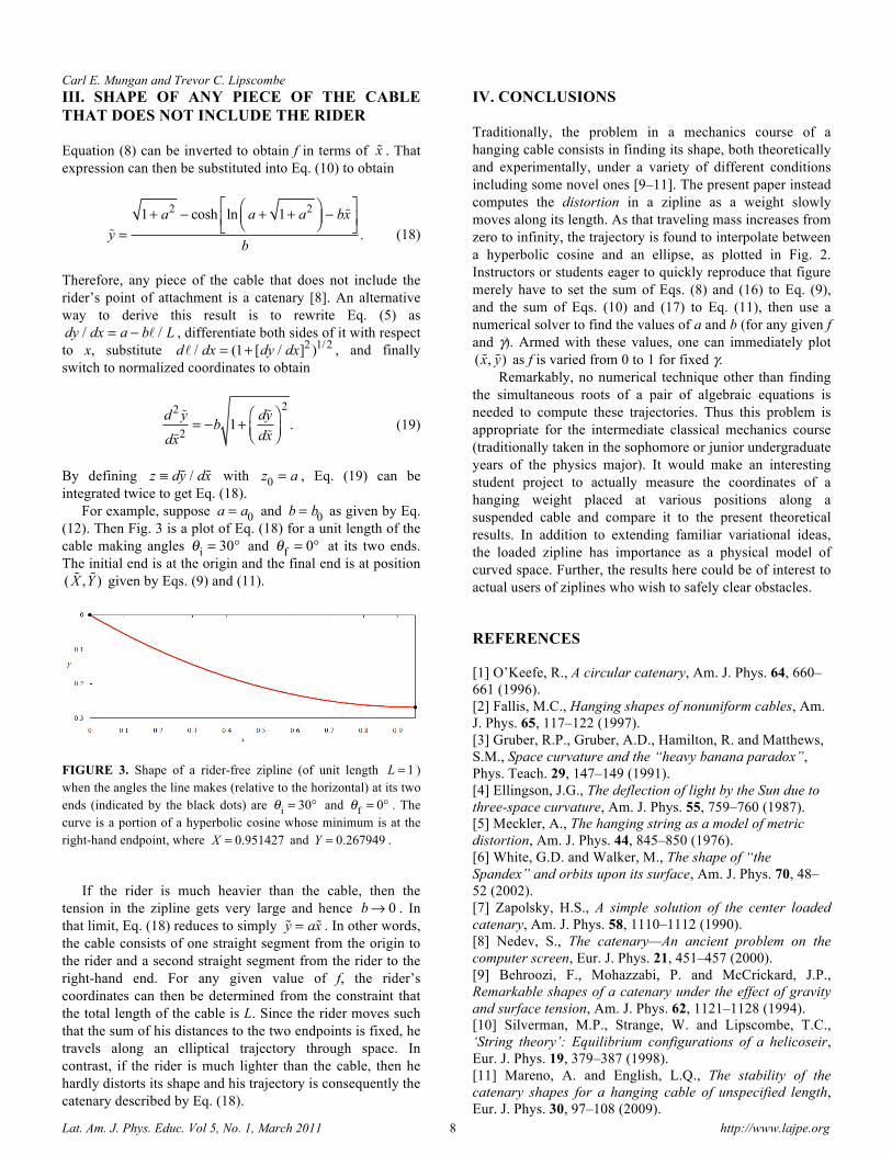
integrated twice to get Eq. (18). For example, suppose

a = a

0 and

b = b

0 as given by Eq.

(12). Then Fig. 3 is a plot of Eq. (18) for a unit length of the cable making angles

!

i= 30° and

!

f= 0° at its two ends.

The initial end is at the origin and the final end is at position

( !X , !Y ) given by Eqs. (9) and (11).

FIGURE 3. Shape of a rider-free zipline (of unit length L = 1 ) when the angles the line makes (relative to the horizontal) at its two ends (indicated by the black dots) are

!

i= 30° and

!

f= 0° . The

curve is a portion of a hyperbolic cosine whose minimum is at the right-hand endpoint, where

X = 0.951427 and Y = 0.267949 .

If the rider is much heavier than the cable, then the tension in the zipline gets very large and hence b! 0 . In that limit, Eq. (18) reduces to simply

!y = a !x . In other words,

the cable consists of one straight segment from the origin to the rider and a second straight segment from the rider to the right-hand end. For any given value of f, the rider’s coordinates can then be determined from the constraint that the total length of the cable is L. Since the rider moves such that the sum of his distances to the two endpoints is fixed, he travels along an elliptical trajectory through space. In contrast, if the rider is much lighter than the cable, then he hardly distorts its shape and his trajectory is consequently the catenary described by Eq. (18).

IV. CONCLUSIONS Traditionally, the problem in a mechanics course of a hanging cable consists in finding its shape, both theoretically and experimentally, under a variety of different conditions including some novel ones [9–11]. The present paper instead computes the distortion in a zipline as a weight slowly moves along its length. As that traveling mass increases from zero to infinity, the trajectory is found to interpolate between a hyperbolic cosine and an ellipse, as plotted in Fig. 2. Instructors or students eager to quickly reproduce that figure merely have to set the sum of Eqs. (8) and (16) to Eq. (9), and the sum of Eqs. (10) and (17) to Eq. (11), then use a numerical solver to find the values of a and b (for any given f and γ). Armed with these values, one can immediately plot

( !x, !y) as f is varied from 0 to 1 for fixed γ.

Remarkably, no numerical technique other than finding the simultaneous roots of a pair of algebraic equations is needed to compute these trajectories. Thus this problem is appropriate for the intermediate classical mechanics course (traditionally taken in the sophomore or junior undergraduate years of the physics major). It would make an interesting student project to actually measure the coordinates of a hanging weight placed at various positions along a suspended cable and compare it to the present theoretical results. In addition to extending familiar variational ideas, the loaded zipline has importance as a physical model of curved space. Further, the results here could be of interest to actual users of ziplines who wish to safely clear obstacles. REFERENCES [1] O’Keefe, R., A circular catenary, Am. J. Phys. 64, 660–661 (1996). [2] Fallis, M.C., Hanging shapes of nonuniform cables, Am. J. Phys. 65, 117–122 (1997). [3] Gruber, R.P., Gruber, A.D., Hamilton, R. and Matthews, S.M., Space curvature and the “heavy banana paradox”, Phys. Teach. 29, 147–149 (1991). [4] Ellingson, J.G., The deflection of light by the Sun due to three-space curvature, Am. J. Phys. 55, 759–760 (1987). [5] Meckler, A., The hanging string as a model of metric distortion, Am. J. Phys. 44, 845–850 (1976). [6] White, G.D. and Walker, M., The shape of “the Spandex” and orbits upon its surface, Am. J. Phys. 70, 48–52 (2002). [7] Zapolsky, H.S., A simple solution of the center loaded catenary, Am. J. Phys. 58, 1110–1112 (1990). [8] Nedev, S., The catenary—An ancient problem on the computer screen, Eur. J. Phys. 21, 451–457 (2000). [9] Behroozi, F., Mohazzabi, P. and McCrickard, J.P., Remarkable shapes of a catenary under the effect of gravity and surface tension, Am. J. Phys. 62, 1121–1128 (1994). [10] Silverman, M.P., Strange, W. and Lipscombe, T.C., ‘String theory’: Equilibrium configurations of a helicoseir, Eur. J. Phys. 19, 379–387 (1998). [11] Mareno, A. and English, L.Q., The stability of the catenary shapes for a hanging cable of unspecified length, Eur. J. Phys. 30, 97–108 (2009).