Transversely anisotropic curved optical fibers: variational analysis of a nonstandard eigenproblem

IEEE TRANSACTIONS ON MICROWAVE THEORY AND TECHNIQUES, VOL. 31, NO. 1, JANUARY 1989 51

Transversely Anisotropic Curved Optical Fibers: Variational Analysis of a

Nonstandard Eigenproblem MARKKU I. OKSANEN AND ISM0 V. LINDELL, SENIOR MEMBER, IEEE

Abstract -A new variational functional is introduced for the analysis of curved open and closed waveguides. The theory is based on the variational principle for nonstandard eigenvalue problems, recently applied for straight anisotropic fibers. The present method is valid for arbitrary waveguide cross section and arbitrary radius of curvature for closed waveguides, but for open guides, the radius should be large enough because the method predicts the real part of the propagation constant, not the imaginary part, which gives the attenuation in curved open structures. The dielectric medium can be homogeneous or nonhomogeneous with transverse and/or longitudinal anisotropy. As an example of the method, curved isotropic and anisotropic single-mode fibers with two different kinds of anisotropy models are studied. The analysis includes field distributions, changes in the dispersion curves due to reformed geometry, and birefringence characteristics in curved anisotropic fibers.

I. INTRODUCTION HE BENDING of an optical fiber or an open dielec- T tric waveguide has been proved to cause radiation

loss, change of the real part of the propagation constant [l], [2], and birefringence, studied particularly in the single-mode optical fibers [3]. The state of the polarization and the field distribution are also modified by the curvature [4], [5]. The loss can be divided into two parts: the pure bending loss due to the uniform curvature and the transition loss related to the mode conversion at the begin- ning of a bend [6]. The attenuation is proportional to Ja/R, exp( - CR,), with C depending on the propagation parameters [l], [7], whereas the phase correction has a ( u / R , ) ~ dependence for waveguides of symmetrical cross section [l]. R , refers to the radius of the bend and a to the characteristic dimension of the waveguide, e.g. the radius of the core in the optical fiber. The bending-induced birefringence is a stress effect [3] which depends on the outer radius d of the waveguide according to (d /Ro)2 . Under the bending the outer portion of the fiber cross section is in tension, which, then, presses laterally on the inner portion, which is in compression [SI. This stress modifies thq refractive index of the fiber material in a very complicated way [ 91 and thus generates birefringence.

Manuscript received October 20, 1987; revised August 8, 1988. This work was supported by grants from the Academy of Finland and the Emil Aaltonen Foundation.

The authors are with the Electromagnetics Laboratory, Faculty of Electrical Engineering, Department of Electronics, Helsinki University of Technology, Otakaari 5A, SF-02150 Espoo, Finland.

IEEE Log Number 8824625.

However, there has also been an attempt to analyze the birefringence purely from the geometrical origin [lo]. Field deformation and the polarization state in a curved slab waveguide [l], [ll], in a rectangular waveguide [ l l ] , [12], and in a curved round fiber [4], [5], [13] have been considered. One important result is that in a fiber the polarization states of all modes except the HE,, modes changes due to fiber axis curvature [4], [13].

A great deal of effort has been expended on various analytical and numerical methods for the open curved waveguides. The fo,llowing review introduces some of these studies in the literature. Most of the methods, e.g. [l], stand on the assumption of a large radius of curvature and thus make use of perturbational technique. An approxi- mate eigenvalue equation for a slab waveguide has been derived [l l] . Other methods for dielectric planar and rectangular waveguides include perturbational analysis [ 141, [U] and the straight waveguide approximation [2], [16]. Spectral expansion techniques [14, [ 171-[20] as well as beam propagation methods [21], [22] can be applied to general open waveguides. A bent open waveguide can be considered a radiating antenna [23], [24] or a straight waveguide with a modified index of refraction through a conformal transformation [12], [26], [27]. An exact numerical analysis in the toroidal coordinate system has also been introduced [28]. Expansions of the slab waveguide theory to include the optical fiber have been carried out [29], [30]. Geometrical optics [31] and analytical loss formulas of the fiber, such as [32], are also available in the literature. One group of reports applies coupled-mode theory to estimate mode conversion in a bent waveguide [SI, [9], [33], 1341. The variational technique has received scant attention among the various methods dealing with curved waveguides. There seems to be only one study based on t h s technique [35]. The purpose of this paper is to introduce a new variational method applicabie to curved open and closed waveguides. The dielectric medium of the waveguide can be inhomogeneous and anisotropic.

Wave propagation in a waveguide can be governed by the following abstract equation [36]:

where L(A) and A stand for the operator and the eigenvalue parameter of the problem, respectively. The problem

L ( A)! = 0 (1)

0018-9480/89/0100-005 1$01 .OO 01 989 IEEE

52 IEEE TRANSACTIONS ON MICROWAVE THEORY AND TECHNIQUES, VOL. 37, NO. I , JANUARY 1989

r I’ I \ ‘

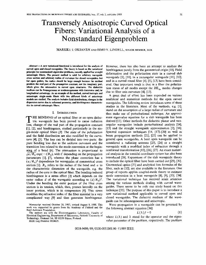
Fig. 1. A uniformly bent anisotropic waveguide and the related coordinate systems.

is called nonstandard if L(X) is a nonlinear function of A; otherwise it is called standard. Boundary conditions asso- ciated with closed waveguides or dielectric boundaries can be hidden in the formula (1) with a suitable choice of the field f or .they can be taken into account by an additional equation. Equation (1) can be solved by a variational method, provided that the inner product

(f, W 4 f ) = 0 ( 2 ) exists. If the operator L is self-adjoint with respect to tlus inner product, (2) possesses stationary roots for A, as was proved in [37]. For the eigenvalue X one can take any possible geometrical or physical parameter involved in the problem. Stationary roots can also be obtained for a given new parameter which has been derived from the old ones.

In Section 11, the formulation of a curved waveguide in terms of the longitudinal fields is seen to lead to a nonstandard eigenproblem (1). With a definition of a proper inner product (2) , a stationary functional is derived. In Section I11 this functional is shown to be a generalization of the former functional for the straight waveguide [36]. In Section IV, the present theory is applied to a bent, weakly guiding step-index fiber. For the trial fields, asymptotic fields derived under the weakly guiding assumption and for large radius of curvatures are used. In Section V, a curved anisotropic fiber with two different lunds of

tion is denoted by U ; . The field components in the two coordinate systems are related by

E,=Epcos8-E,sin8 E , = Epsin8+E,cos8. (7)

We assume a field formulation E ( R , Z)exp(- jv+) or E(p, B)exp( + jps) with time dependence exp(jwr) omitted. Curl operators in the local ( I ) and global ( 8 ) coordinate systems are related to each other by

(V X A ) R = ( V X A ) , + A , u , / R (8)

where subscripts g and 1 stand for the transverse differential operator obtained by setting d / d + (g) or a / a s ( I ) equal to zero in the two coordinate systems, respectively. The gradient operator is invariant with respect to the coordinate system: (of), = (of),. For the partial de- rivatives we have d/dR = COS 8a/dp - sin 8a/p a 8 and a/az = ~ 0 ~ 8 a / ~ a e + sinealap.

The waveguide is modeled by a symmetric dielectric dyadic

4 P ) = + I + E , ( P ) U , U , ( 9 4

where c( p ) = E , ( p)u,u, + E , ( p)u,u, is a two-dimensional dyadic in the transverse plane xy with a position vector p and orthogonal vectors U”, U , in that plane. The dielectric medium will be assumed lossless. In open guides the bend generates compressional strain, which changes permittivity. For an optical fiber these fractional increases in those directions, x and y , which contribute to the propagation characteristics of the waveguide have been estimated to be of the order of 0.0015(d/R0)4~ and 0 . 0 1 8 ( d / R 0 ) 4 ~ [34], where d is the outer diameter of the fiber. To add these additional terms S E X , Scy to the formula (sa) results in the following permittivity matrix:

E + O I

E , + S E , cos2 a + S E sin2 a ( S E , - S E , ) sin a cos a

( S E , - S E , ) sinacos a E , , + S E , C O S ~ ~ + sin2a o 0 0

anisotropy models is analyzed. Section VI contains the conclusions of this paper.

11. THEORY

We consider a bent anisotropic waveguide with a radius of curvature R , in the global cylindrical coordinate system (0, R , +, Z), Fig. 1. The guiding direction is along the axis of the waveguide, which is the s axis of the local toroidal coordinate system (0’, p, 8, s) or (0’, x, y , s). The two coordinate systems are related by the following equations:

R = R o + p c o s 8 = pcose (3)

Z=ps inB= y (4)

S/RO. ( 5 ) ( p -

which is still symmetric. a is the angle between U , and U ,

vectors. As in [36], we derive equations for the longitudinal

fields. We start by writing the guided fields in the global coordinate system as E ( R , Z)exp(- jv+) = ( e ( R , Z ) + e( R , Z ) U + ) exp ( - jv+) and H ( R , Z ) exp ( - jv@) =

( h ( R , Z ) + h ( R , Z)u,)exp(- jv+) and then insert them in Maxwell’s equations. After some algebra we are left with the following equations

(10)

(11)

(12)

v x e + jwphu, = 0

v x h - jwc+eu, = 0

v ( e R ) X U , + j v e X U , + j w p m = 0

In each coordinate system, the unit vector in the i direc- v ( h R ) X u , + j v h X u , - j o R c . e = O . (13)

OKSANEN AND LINDELL: TRANSVERSELY ANISOTROPIC CURVED OPTICAL FIBERS

~

53

Here U, is the axial unit vector, whence for the transverse fields we have u+.e = 0 and U,-h = 0. The curl operator denotes a transverse differential operator. From (12) and (13) we eliminate the transversal field vectors e and h:

(14) e = - j k ; ’- [ vv ( R e ) / R 2 + wpv ( Rh ) X u + / R ]

h = ju, X kL2. [ - o c . v ( R e ) / R + vu, X v ( R h ) / R 2 ] .

(15)

-

Next we assume the boundary of the waveguide to be a perfect conductor, and assume the fields to obey the corresponding boundary conditions. This assumption sim- plifies the derivation of the functional, but causes a small error for the propagation parameters when the functional is applied to the open waveguides. This will be discussed later.

The operator L operates on the pair of scalar functions ( e , h) according to

wu,.v X [ k ; ’ . c . ~ ( e R ) X u , / R ] - w c ~ e - v u + . V X [ ( k , Z ~ u , u , ) . V ( R h ) / R 2 ]

VU,-V X [ kF2-v ( R e ) / R 2 ] - oph + wpu,*V X [ kF2-V ( h R ) X u , / R ]

Here kL2 is the inverse of the two-dimensional dyadic

kz = w2pe - ( v / R ) ~ E (16) and E is the two-dimensional unit dyadic: E = I - u+u,. The inverse dyadic can be defined as [36]

k i 2 = ( k z u,u+)/spm( kz).

The definition of the double cross product here is as follows: (ab) :: (cd) = ( a X c)(b X d) and spm( ) is the two-dimensional determinant function (sum of principal minors of the three-dimensional dyadic) defined by spm A = A CA : 1/2. Inserting (16) into (17) and using the above definition for spm( ) gives us the inverse dyadic

k;’ = k;:u,u, + k;:U,U, (18)

where the components are

kS2 = ( w2pci - ( v / R ) ~ ) - ‘ , i = U , w . (19)

The equations for the longitudinal fields can now be written by substituting (14) and (15) into (10) and (11). After rearranging terms and using vector analysis, we obtain

V X (U, X k i 2 . [ - w e . v ( e R ) / R + vu, X v ( R h ) / R 2 ] )

- oc+eu+ = 0 (20)

v X ( k ; ’- [ vv ( e R ) / R 2 + wpv ( hR ) X u J R ] ] - wphu+ = 0. (21)

These equations form the basis for the present theory. In order to apply the variational method, we have to define a proper inner product (2) and the operator L(X) in (1) which is self-adjoint with respect to that inner product. These requirements can be satisfied by the following definitions. The unknown fields are longitudinal fields ( e , h), which we denote here by f as in (1) and (2), and define the following inner product ( , 0 ) :

To verify that the above definitions lead to a self-adjoint formulation, we form the inner product according to (22)

(f,,Lf2) =.- ~ / { c , e l e ’ + P h , h 2 } dS

+ UP/( (V(h1R) X U + / R )

+ a/( ( ( e & X U + / 4

- k ; ’ * ( v ( h 2 R ) X u , / R ) ) dS

. k ; ’ . e . ( V ( e , R ) x u , / R ) ) dS

+ v/( V( h , R ) / R - (U, X k i 2 )

. v ( e 2 R ) / R 2 +v(h2R)/R2 -(U, X k;’) -v( e , R ) / R ] dS = 0 (24)

where the divergence terms, reduced to line integrals at the boundary of the waveguide, do not contribute because of the assumed requirement for the fields. To be self-adjoint, (24) should be symmetric in 1 and 2. The first term is clearly symmetric and so are the second and third terms, provided that the dyadic e is symmetric, as was assumed in (9a) and (9b). The last terms are not symmetric; instead they form a symmetric pair. As a conclusion, L is self- adjoint and we can apply the functional (2) written for this special problem in (24).

The operator L, defined in (23) contains the dyadic kL2, which is a complicated function of all the physical parameters involved in the problem. Bearing this in mind, there is no hope of solving the functional (24) explicitly for any of the parameters. This is evidently true also for any possible geometrical parameters, which can be included in the permittivity dyadic e. Thus the eigenvalue equation Lf = 0 is of a nonstandard type [37]. To overcome difficulties involved in this kind of problem we proceed analogously to [36] and define new parameters from the old ones and try to solve the functional in terms of these. In fact, forming a two-dimensional dyadic as M = w2kF2/R2

= ( R 2 p c , - y - 2 ) - 1 ~ u u u + ( R 2 p c w - Y - ~ ) - ~ u , u , (25) where we have defined a new parameter y as

y = w / v (26)

54 IEEE TRANSACTIONS ON MICROWAVE THEORY AND TECHNIQUES, VOL. 31, NO. 1, JANUARY 1989

we can express the functional (24) in a compact form for the parameter w2:

I{ v( R e ) . M - e . v ( Re) + (U+ X V ( R h ) ) . M p - ( U+ X V ( R h ) ) -2u+ X V ( R h ) - M . V ( R e ) / ( R y ) } dS

/ { r+e2+ph2) d~ (27) J =

where the integration extends over the waveguide cross section. Equation (27) is a stationary functional for w2. The above derivation could have been carried out in terms of the transversal fields, whence the functional would have been of the standard form in both w2 and P2. However, the operator L would then be non-self-adjoint with respect to the symmetric inner product applied here and the proper solution would also require the adjoint problem to be taken into account, as was noted in [38] for the case of the straight corrugated waveguide.

The functional (27) is exact for the closed curved waveguides, and can handle an arbitrary radius of curvature. The only requirements for the fields are continuity every- where and ideal conductor conditions for the fields at the waveguide boundary. The dielectric tensor can be arbitrary provided that it is symmetric. With these comments the above equation is the most general functional for closed bent waveguides and, to the knowledge of the authors, has not been introduced before. For the isotropic waveguide, the functional takes on the simplified form

larger than the imaginary part because here the dependence is of the order (a/Ro) ' [l].

111. TESTING THE FUNCTIONAL: THE RADIUS OF CURVATURE -9 CO

As the radius of curvature R , in (3) goes to infinity, the torodial coordinate system straightens to the cylindrical one with coordinates p , 8 , and s. Then the following transformations hold:

v / R + V/R , -9 Po

Ry = Rw/v + Roo/v = o/Po = up

~ - 9 ~ : , ( ~ ~ " - - ( ~ / ~ ~ ~ ) ~ ) - ~ u , u ,

(29)

(30)

+ = R ~ ( ( p r , - u ~ Z ) - 1 u , u , + ( p ~ , - u ~ 2 ) ~ 1 u , u , )

= R;N (31)

When the waveguide is open, such as in the optical fiber, the functional can be used only as an approximation. This comes from the different boundary conditions. If the open guide is bent, it becomes radiative, and the fields at

where up refers to the phase velocity of the field and N is a two-dimensional dyadic.

Inserting (29)-(31) into (27) and taking the limit as R + 00 gives US

infinity are nonzero. Then the line integrals must be added in (24), and the functional includes additional terms. How- ever, if we assume the radius of curvature to be sufficiently large, so that the attenuation is very small due to the exponential decay [l], [7], the functional (27) can be applied to estimate the change of the real part of the propagation constant due to the bending. This part is essentially

This is identical with the functional for the straight open waveguide [35]. The trial fields are now exponentially decaying as p + CO. Unfortunately, the functional in [36] is not written correctly. The coefficient in the last term in the functional should read -2/up and not -2.

The same limiting process can be performed for the isotropic guide, whence we obtain

(33)

OKSANEN AND LINDELL: TRANSVERSELY ANISOTROPIC CURVED OPTICAL FIBERS 55

which again is identical with that derived in [36] for the straight isotropic waveguide.

IV. THE BENT ISOTROPIC STEP-INDEX FIBER As a first example we consider a weakly guiding isotropic

step-index optical fiber bent by a radius of R , (Fig. 1). Here we treat the fiber purely from the geometrical point of view. This means that small changes in dielectric prop- erties of the fiber due to the bending are ignored. Also, the linear birefringence resulting from this modified permittivity is not taken into account. From the optical waveguide theory we adopt the usual notations for the normalized frequency V , normalized propagation constant b, and parameter A , the normalized dielectric constant difference between the core and the cladding of the fiber:

V = q / - = k 2 a a (34)

( 3 5 )

(36)

Here, 1 stands for the medium in the core and 2 for that in the cladding. The radius of the core is denoted by a. The propagation constant /3 is related to the azimuthal index v and the radius R, according to p = v / R , , which we ex- pand as a power series:

p2 = p i + p"( C X / R , ) ~ + (37) where Po denotes the propagation constant of the straight fiber and a = p;u3/4. In the weakly guiding fiber we have a = V 2 a / 4 A . The term proportional to ( l / R o ) is missing in the expansion. This has been noted in many asymptotic studies of the curved waveguide when the waveguide possesses a symmetric structure with certain symmetry proper- ties of the mode fields, e.g. [ l ] and [39]. This holds as well for closed waveguides [40] and for symmetric dielectric slab waveguides [ l ] . The expansion is valid only for large radius of curvature. If the radius becomes small, the con- vergence is very poor, and the propagation constant has a Rg2I3 dependence [41].

The dielectric function can be written from (36) as

4) = E2(1+ A P ( P ) ) (38) where P ( p ) is the pulse function for the step-index fiber: P( p ) = 1 for p G a, and = 0 for p > a.

Field deformation in a curved step-index fiber has been solved by a numerical method using Fourier-Bessel series expansions [ 51. Analytical equations for the transversal fields have been derived by applying a first-order perturbation theory [4] . In [13] the theory was extended to include radially inhomogeneous fibers and longitudinal fields. Studies based on a Gaussian function approximation for the fields have been published [42], [43]. Field deformation can cause a significant contribution to the radiation loss of the fiber, as was noted in [32]. Here we derive longitudinal fields in the curved fiber starting from (20) and (21), which

we take for the isotropic waveguide. The resulting field equations are similar to those in [13].

After rearranging terms in (20) we are left with an equation for the longitudinal field in the curved waveguide:

e 2vk2 2v2 v ?e - - + k:e + ~ 8 h /aZ - - 8 ( R e ) / d R = 0

R2 ucR2kz R4k;

(39)

where k ; = k 2 - ( p R o / R ) 2 and v = P R O . The corresponding equation for the magnetic field can be obtained by changing e to h and c to - p and vice versa. Equation (39) is exact and contains no approximations. To solve it we apply a perturbational method where the solution can be sought as a power series in R,, assuming

e = e, + e , a / R , + e 2 ( a / R , ) + . . . . (40) By inserting (37) and (40) into (39) and equating powers of R , we obtain a set of differential equations for the field e.

2

The zero-order equation reads

v : e , + ( k 2 - # ) e , = 0 (41)

where v: denotes the transverse Laplace operator and k 2 = k;(1+ AP) . The first-order equation is

and c = c 2 d m . In the weakly guiding waveguide we have approximately Po = k .

By solving (41) we have, for the lowest order HE,, mode,

Jl( w / a ) /Jd 4 cos (0 - 8,) for p G a

K,( w p / u ) / ~ , ( w ) cos (e - e,) for p > a . e,= { (43)

J and K denote the Bessel and modified Hankel functions, respectively. 0, is the polarization angle: 0, = 0" and 0, =

90" correspond to the mode polarized in the x and the y direction, respectively. U and w are the normalized parameters, defined as u2 = ( k ; - P:)a2; w 2 = (P i - k : ) a 2 . In terms of the normalized frequency and propagation constants we have U = and w = V&. The normalized parameter bo is the solution of the eigenvalue equation at the limit A + 0: u J , ( u ) / J 0 ( ~ ) = wK,(w)/K,(w)

If we denote the radial dependence of the zero-order [441-

solution e, by t ( p ) , the corresponding magnetic field is h , = Ht ( p ) sin ( e - e,) (44)

where H is the magnetic field coefficient, which can be approximated by H = for the HE,, mode under the weakly guiding assumption [44]. The same value for H can also be obtained by optimizing the functional (33) with respect to this parameter, as was demonstrated in [36].

56 IEEE TRANSACTIONS O N MICROWAVE THEORY A N D TLCHNIQIJES. VOL. 37. NO. 1. JANIJARY 1 Y x Y

The first-order fields are solutions of (42). They are, with the assumption Po = k ,

( ( ( + ( P/u)2u - 1 ) JO + 2( p/. ) J,U - 2 ) /J,( U ) cos 8"

The error in the field equations due to the above assumption is at most of the order A . The arguments u p / a and wp/a of the special functions in the denominators are omitted. 6 and U are constants derived from the boundary conditions: 6 = - K2( w ) / u K o ( w); U = J2( u) /wJ,(u) .

Analogously to (44), we write e , = f (p) cos 8, + g(p)cos(28 - do). This gives us the magnetic field h,:

h, = H ( -f(p)sind0 + g(p)sin(28 - d o ) ) . (46)

To combine the field classification we write, for the HE,,, mode,

e = t ( P ) cos 0 + ( a /Ro) ( f ( P ) + kd P 1 cos 28 )

h = H(t(p)s ind +(a/RO)g(p)sin28) (47)

and for the HE,,, mode,

e = t(p)sind + (a/RO)g(p)sin28

h = - H ( t ( P ) c o s ~ + ( ~ / R o ) ( f ( P ) $ - g ( P ) c o s 2 ~ ) )

In the weakly guiding limit we have a = P,'u3/4 = V'u/4A. The following relations hold between the mode fields:

e " = h'/H h ' / H = - e ' (48)

where the subscripts x and y denote the HE,,, and HE,,, modes, respectively.

The dispersion relation in the curved fiber can now be calculated from the stationary functional (28), which we express in terms of the normalized parameters I/, b, and A . The parameter b is a function of the propagation constant ,8, so we write

b = b, + b'( a/R,V)'+ . . . = bo + Sb. (49)

Here Sb stands for the change of the normalized parameter and is approximated by the second term b'( Va/4AR,)2 of the asymptotic series. The first-order correction is missing due to the expansion (37). In the weakly guiding limit

A --* 0, the functional reads, in the local coordinate system,

F( P , b o ) = 1 + ( R o A ) '2p cos e / ( P - bo)

The functional is independent of the wave polarization in the weakly guiding limit for the HE,, mode. This is seen by inserting field relations (47) into (50), in which case the integrands remain unchanged. This means that the bend induces the same change in the propagation constants of the orthogonal polarized waves of the HE,, mode. This has been observed previously by many authors applying a variety of methods, e.g. [18].

The unknown parameter Sb is hidden in the functional in a complicated way. To solve this, we can either apply an asymptotic method or make use of some numerical algo- rithm. In the latter, we start from a definite (V . bo) point in the dispersion curve, insert the field expressions, and seek a proper value for Sh so that (50) is satisfied. In the former method we equate coefficients of equal powers of ( a / R , ) in (50). The lowest order equation is

Here, the prime denotes the first derivative of the function with respect to p. This is the functional equation for the straight fiber derived in [36] and gives the corresponding eigenvalue equation by using the longitudinal fields (43). The first-order equation is lacking, which is evident from the asymptotic nature of the propagation constant. The second-order equation gives an expression for the change of the propagation constant ab:


Y

1 2 3 4 5 6 V

Ro = - Robla = 20 R,nla = 50 RoA/a = 80

3 3 4 b0 6bx10 6bxlO 6bxlO

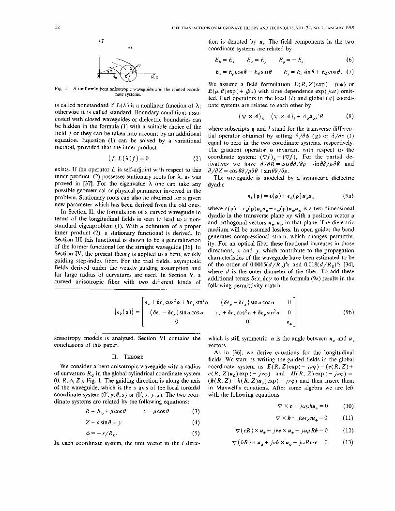
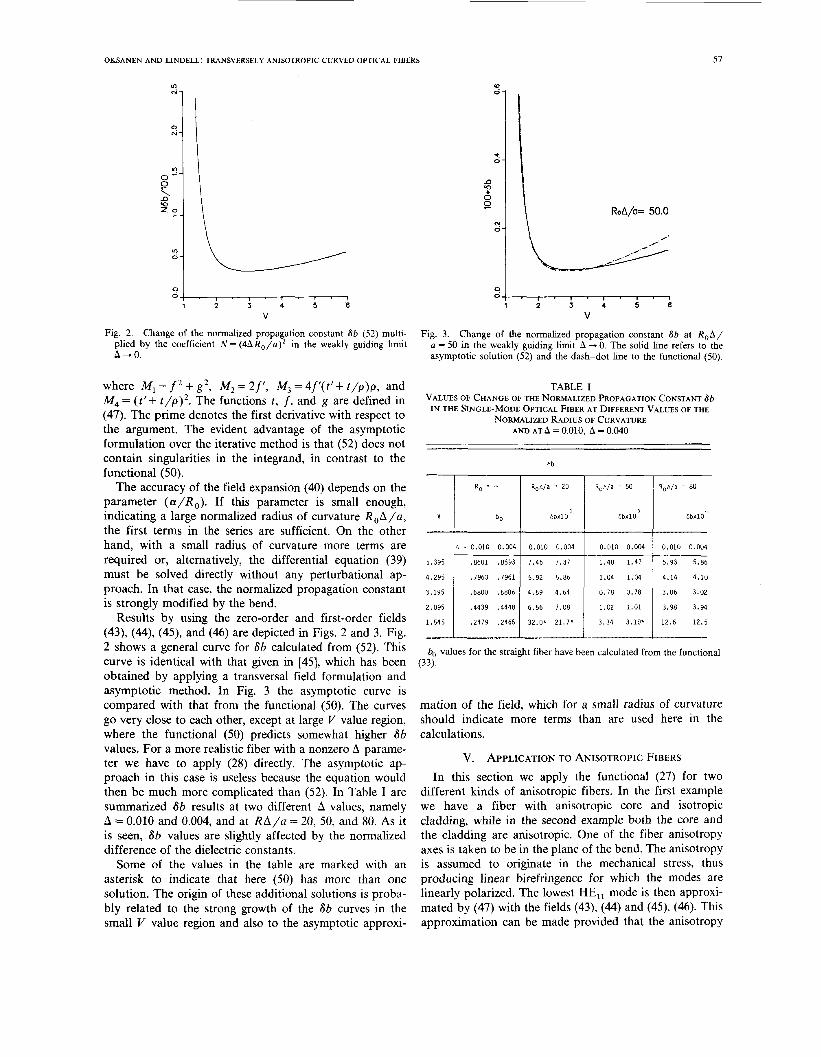
Fig. 2. Change of the normalized propagation constant 6b (52) multiplied by the coefficient N = (4AR,,/a)* in the weakly guiding limit A-0.

where M,= f 2 + g 2 , M2=2f’ , M3=4f’(t’+t/p)p, and M4 = (t’+ t / ~ ) ~ . The functions t, f , and g are defined in (47). The prime denotes the first derivative with respect to the argument. The evident advantage of the asymptotic formulation over the iterative method is that (52) does not contain singularities in the integrand, in contrast to the functional (50).

The accuracy of the field expansion (40) depends on the parameter ( a / R o ) . If this parameter is small enough, indicating a large normalized radius of curvature R o A / a , the first terms in the series are sufficient. On the other hand, with a small radius of curvature more terms are required or, alternatively, the differential equation (39) must be solved directly without any perturbational ap- proach. In that case, the normalized propagation constant is strongly modified by the bend.

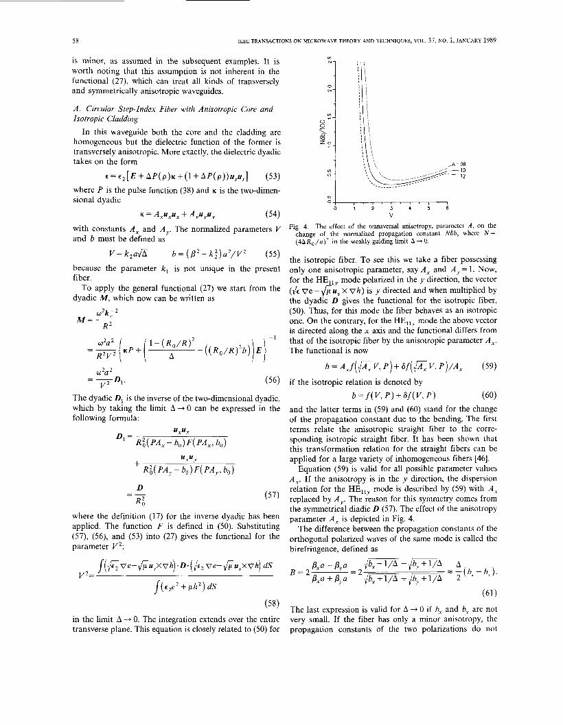
Results by using the zero-order and first-order fields (43), (44), ( 4 9 , and (46) are depicted in Figs. 2 and 3. Fig. 2 shows a general curve for 6b calculated from (52). This curve is identical with that given in [45], which has been obtained by applying a transversal field formulation and asymptotic method. In Fig. 3 the asymptotic curve is compared with that from the functional (50). The curves go very close to each other, except at large V value region, where the functional (50) predicts somewhat higher 6b values. For a more realistic fiber with a nonzero A parameter we have to apply (28) directly. The asymptotic ap- proach in this case is useless because the equation would then be much more complicated than (52). In Table I are summarized 6b results at two different A values, namely A = 0.010 and 0.004, and at R A / a = 20, 50, and 80. As it is seen, 6b values are slightly affected by the normalized difference of the dielectric constants.

Some of the values in the table are marked with an asterisk to indicate that here (50) has more than one solution. The origin of these additional solutions is proba- bly related to the strong growth of the 6b curves in the small V value region and also to the asymptotic approxi-

*. 0-

n

d 9

W

N 0-

V

Fig. 3. Change of the normalized propagation constant 66 at R o d / a = 50 in the weakly guiding limit A + 0. The solid line refers to the asymptotic solution (52) and the dash-dot line to the functional (50).

TABLE I VALUES OF CHANGE OF THE NORMALIZED PROPAGATION CONSTANT Sh

IN THE SINGLE-MODE OPTICAL FIBER AT DIFFERENT VALUES OF THE NORMALIZED RADIUS OF CURVATURE

AND AT A = 0.010, A = 0.040

In = 0.010 0.004 1 0.010 0.004 I 0.010 0.004 I 0.010 0.004

0.78 0.78

1.02 1.01

h,, values for the straight fiber have been calculated from the functional (33 ) .

mation of the field, whch for a small radius of curvature should indicate more terms than are used here in the calculations.

v. APPLICATION TO ANISOTROPIC FIBERS In this section we apply the functional (27) for two

different kinds of anisotropic fibers. In the first example we have a fiber with anisotropic core and isotropic cladding, while in the second example both the core and the cladding are anisotropic. One of the fiber anisotropy axes is taken to be in the plane of the bend. The anisotropy is assumed to originate in the mechanical stress, thus producing linear birefringence for whch the modes are linearly polarized. The lowest HE,, mode is then approximated by (47) with the fields (43), (44) and (49 , (46). This approximation can be made provided that the anisotropy

58 I E E E TRANSACTIONS ON MICROWAVE THEORY A N D T E C H N I Q U E S , VOL. 37, NO. 1, JANUARY 1989

is minor, as assumed in the subsequent examples. It is worth noting that this assumption is not inherent in the functional (27), which can treat all kinds of transversely and symmetrically anisotropic waveguides.

A . Circular Step-Index Fiber with Anisotropic Core and Isotropic Cladding

In this waveguide both the core and the cladding are homogeneous but the dielectric function of the former is transversely anisotropic. More exactly, the dielectric dyadic takes on the form

E = c 2 [ E + AP(p)K + ( I + AP(p))u,u,] (53) where P is the pulse function (38) and K is the two-dimensional dyadic

K = A,u,u, + A,u,u, (54) with constants A , and A,. The normalized parameters V and b must be defined as

V = k 2 a f i b = ( P 2 - k 2 ) a 2 / V 2 ( 5 5 )

because the parameter k , is not unique in the present fiber.

To apply the general functional (27) we start from the dyadic M , which now can be written as

The dyadic D, is the inverse of the two-dimensional dyadic, which by taking the limit A + 0 can be expressed in the following formula:

uxux

Ri( f ‘A , - bo)F(PA,, bo) D, =

vu, + R i ( P A . , - bO)F(PA,, bo)

D =-

R i (57)

where the definition (17) for the inverse dyadic has been applied. The function F is defined in (50). Substituting (57), (56) , and (53) into (27) gives the functional for the parameter v*:

!( c2e2 + p h 2 ) dS

( 5 8 )

in the limit A 4 0. The integration extends over the entire transverse plane. This equation is closely related to (50) for

0 1 2 3 4 5 6

V

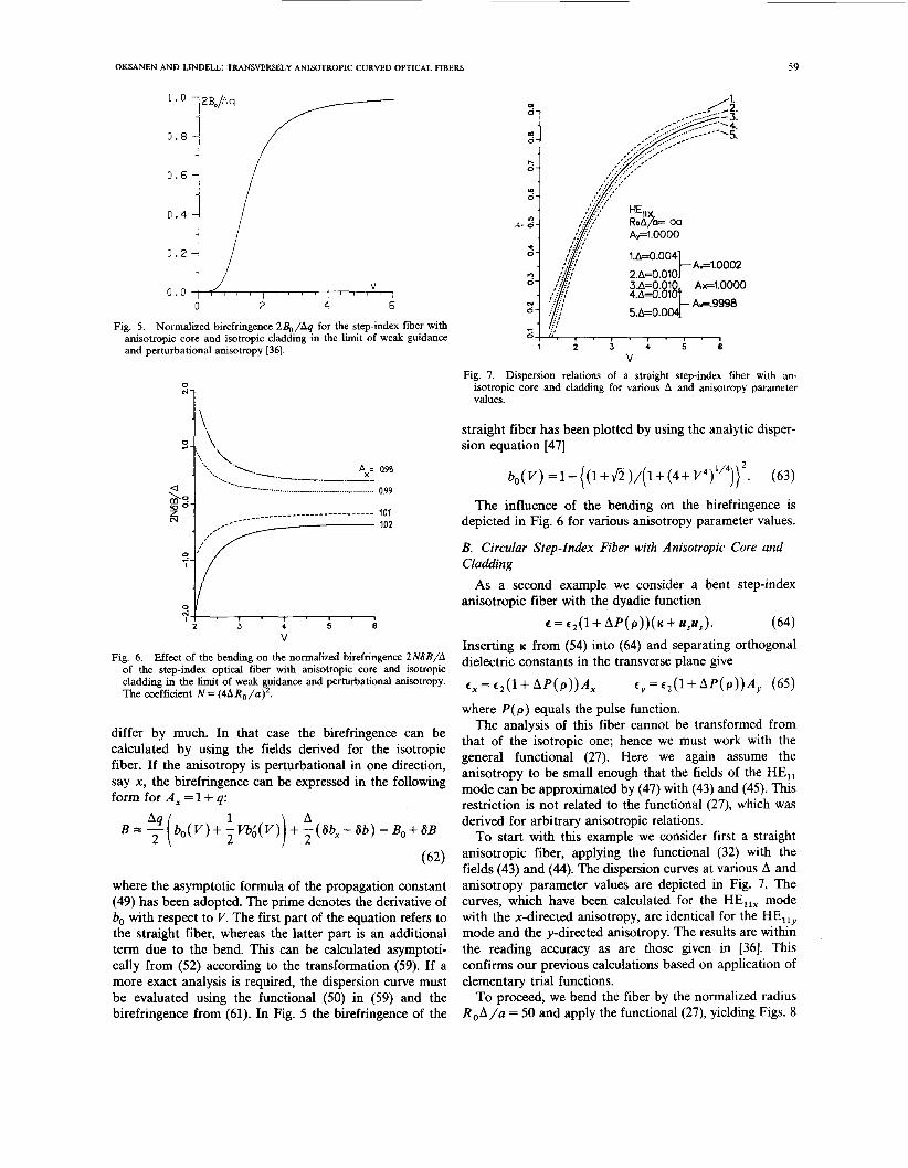
Fig. 4. The effect of the transversal anisotropy, parameter A , on the change of the normalized propagation constant N&b, where N = (4AR,/a)’ in the weakly guiding limit A + 0.

the isotropic fiber. To see th s we take a fiber possessing only one anisotropic parameter, say A , and A , = 1. Now, for the HE,,, mode polarized in the y direction, the vector ( h o e - f i u , X v h ) is y directed and when multiplied by the dyadic D gives the functional for the isotropic fiber, (50). Thus, for this mode the fiber behaves as an isotropic one. On the contrary, for the HE,,, mode the above vector is directed along the x axis and the functional differs from that of the isotropic fiber by the anisotropic parameter A,. The functional is now

if the isotropic relation is denoted by

b = f( v, P) + S.f( v, P) (60) and the latter terms in (59) and (60) stand for the change of the propagation constant due to the bending. The first terms relate the anisotropic straight fiber to the corresponding isotropic straight fiber. It has been shown that this transformation relation for the straight fibers can be applied for a large variety of inhomogeneous fibers [46].

Equation (59) is valid for all possible parameter values A,. If the anisotropy is in the y direction, the dispersion relation for the HE,,, mode is described by (59) with A , replaced by A,. The reason for t h s symmetry comes from the symmetrical diadic D (57). The effect of the anisotropy parameter A , is depicted in Fig. 4.

The difference between the propagation constants of the orthogonal polarized waves of the same mode is called the birefringence, defined as

p,a-~,,a /w-/w A B = 2 p,a+p,a =2/b,’+/w = - 2 ( b, - b, ) .

(61 1 The last expression is valid for A + 0 if b, and b,, are not very small. If the fiber has only a minor anisotropy, the propagation constants of the two polarizations do not


0 . 8 -

0 . 6 -

0.4 -

0.2 -

0 . 0

59

v I I I T , I I I I 1 4 I I I I

R l \

s y . , . , . , . 2 3 4 5 6

v Fig. 6 . Effect of the bending on the normalized birefringence 2N6B/A

of the step-index optical fiber with anisotropic core and isotropic cladding in the limit of weak guidance and perturbational anisotropy. The coefficient N = (4ARo/a)*.

differ by much. In that case the birefringence can be calculated by using the fields derived for the isotropic fiber. If the anisotropy is perturbational in one direction, say x , the birefringence can be expressed in the following form for A, =1+ 4:

(ab, - 6b) = Bo + 6B

where the asymptotic formula of the propagation constant (49) has been adopted. The prime denotes the derivative of bo with respect to V. The first part of the equation refers to the straight fiber, whereas the latter part is an additional term due to the bend. This can be calculated asymptotically from (52) according to the transformation (59). If a more exact analysis is required, the dispersion curve must be evaluated using the functional (50) in (59) and the birefringence from (61). In Fig. 5 the birefringence of the

A~1.0002 2.A=0.010 3.A=0.010, A~ l .0000 4.A=0.010 5.A=O.O

Ar.9998

O ] i;. , . , . , . , . , 1 2 3 4 5 6

V Fig. 7. Dispersion relations of a straight step-index fiber with an-

isotropic core and cladding for various A and anisotropy parameter values.

straight fiber has been plotted by using the analytic dispersion equation [47]

bo( V ) =1-( (1 +&)/(l+ (4-t V4)1'4))2. (63)

The influence of the bending on the birefringence is depicted in Fig. 6 for various anisotropy parameter values.

B. Circular Step-Index Fiber with Anisotropic Core and Cladding

anisotropic fiber with the dyadic function As a second example we consider a bent step-index

z = c2(1 + AP( p ) ) ( K + usus). (64) Inserting K from (54) into (64) and separating orthogonal dielectric constants in the transverse plane give

e, = € 2 0 + AP(P) )A, c y = € 2 0 + AP(P) )A, (65)

where P( p ) equals the pulse function. The analysis of this fiber cannot be transformed from

that of the isotropic one; hence we must work with the general functional (27). Here we again assume the anisotropy to be small enough that the fields of the HE,, mode can be approximated by (47) with (43) and (45). This restriction is not related to the functional (27), which was derived for arbitrary anisotropic relations.

To start with this example we consider first a straight anisotropic fiber, applying the functional (32) with the fields (43) and (44). The dispersion curves at various A and anisotropy parameter values are depicted in Fig. 7. The curves, which have been calculated for the HE,,, mode with the x-directed anisotropy, are identical for the HE,!, mode and the y-directed anisotropy. The results are withm the reading accuracy as are those given in [36]. This confirms our previous calculations based on application of elementary trial functions.

To proceed, we bend the fiber by the normalized radius R o A / a = 50 and apply the functional (27), yielding Figs. 8

60 IEEE TRANSACTIONS ON MICROWAVE THEORY AND TECHNIQUES, VOL. 37, NO. 1, JANUARY 1989

1 2 3 4 5 6

RoA/b= 50.0 8

l . I ' , . 1 2 3 4 5 6

v V

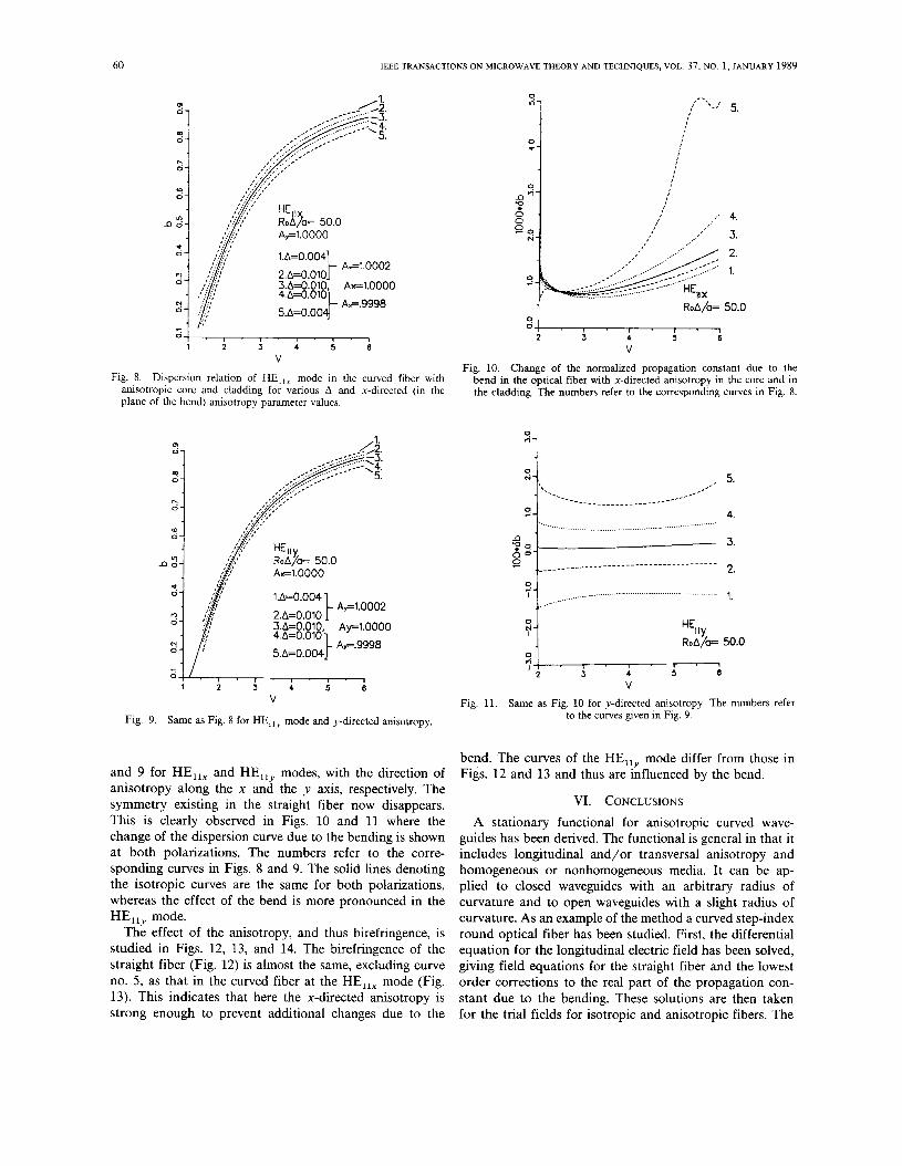
Fig. 10. Change of the normalized propagation constant due to the bend in the optical fiber with x-directed anisotropy in the core and in the cladding. The numbers refer to the corresponding curves in Fig. 8.

Fig. 8. Dispersion relation of HE,,, mode in the curved fiber with anisotropic core and cladding for various A and x-directed (in the plane of the bend) anisotropy parameter values.

Fig. 9.

m

x -1 A~1.0000

1 2 3 4 5 6

V

Same as Fig. 8 for HE,,, mode and y-directed anisotropy

and 9 for HE,,, and HE,,, modes, with the direction of anisotropy along the x and the y axis, respectively. The symmetry existing in the straight fiber now disappears. This is clearly observed in Figs. 10 and 11 where the change of the dispersion curve due to the bending is shown at both polarizations. The numbers refer to the corresponding curves in Figs. 8 and 9. The solid lines denoting the isotropic curves are the same for both polarizations, whereas the effect of the bend is more pronounced in the HE,,, mode.

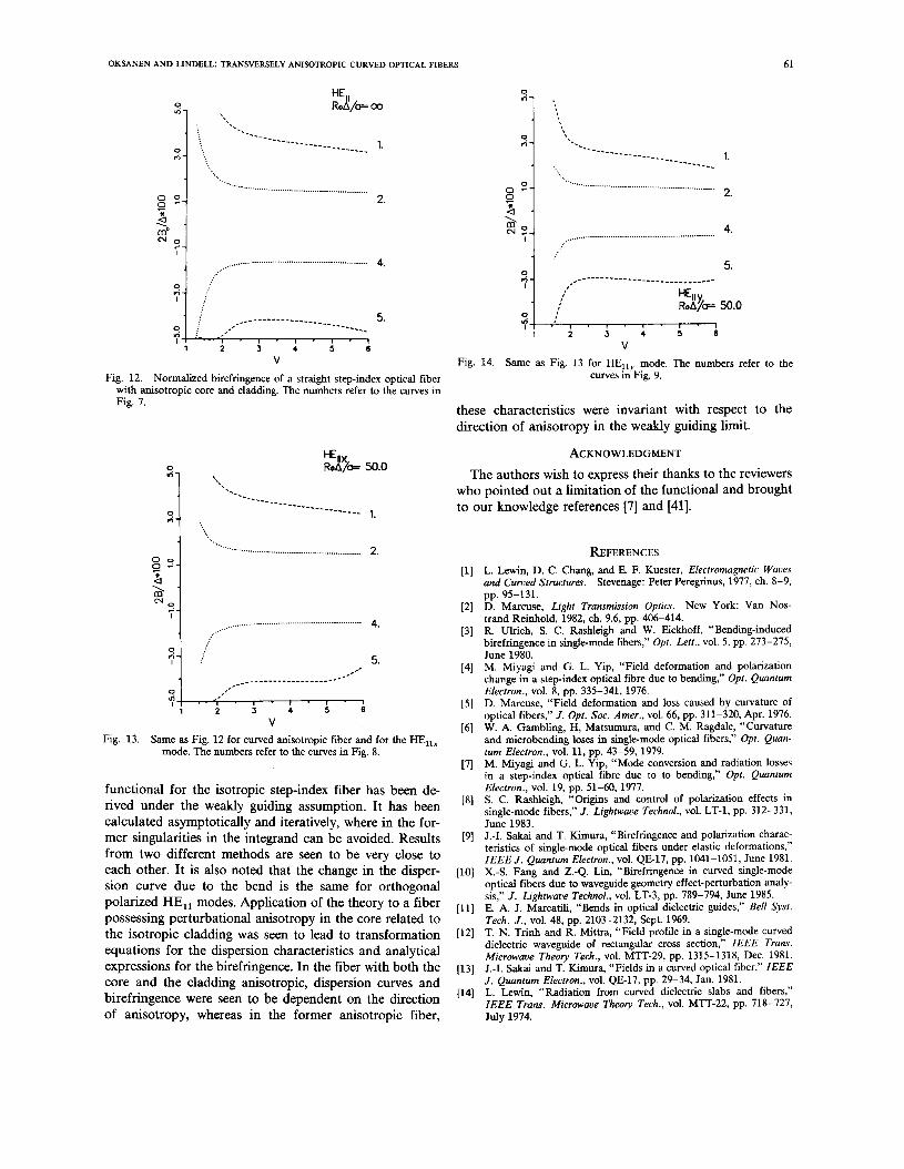
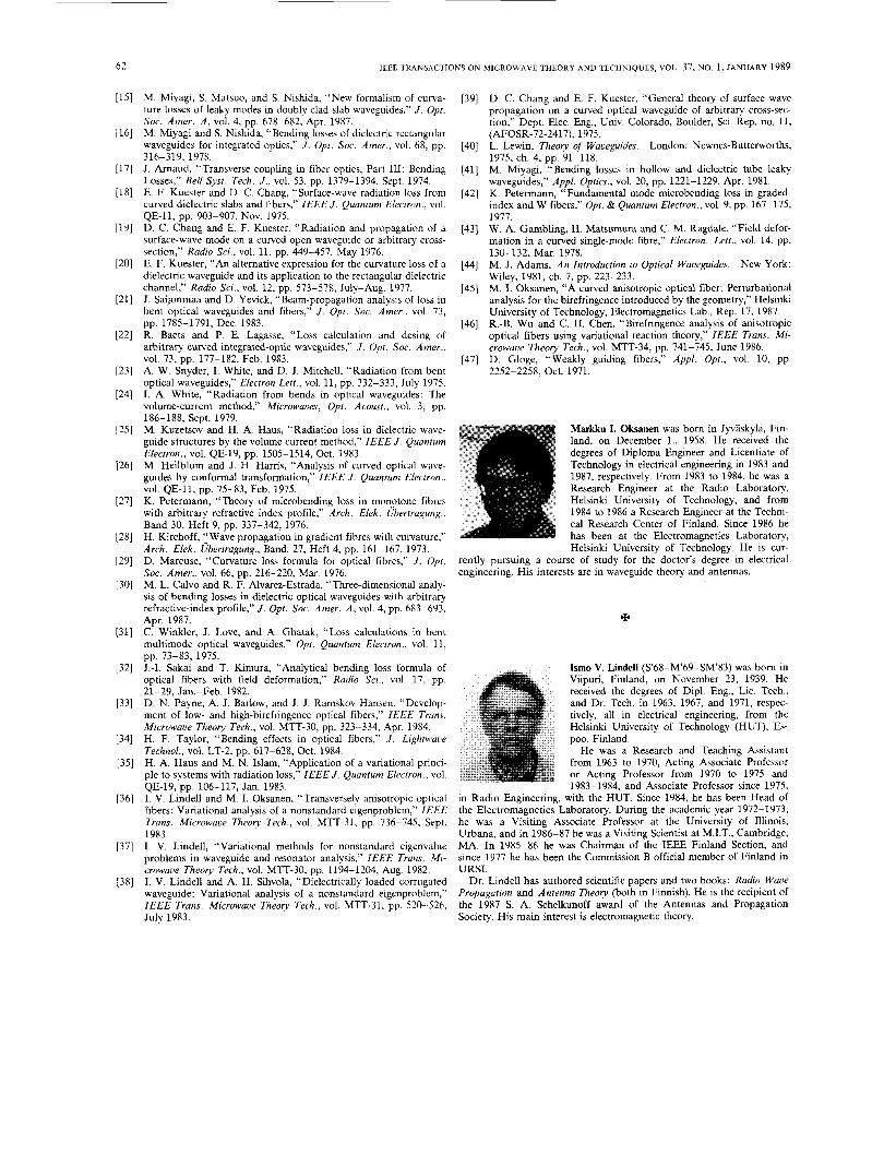
The effect of the anisotropy, and thus birefringence, is studied in Figs. 12, 13, and 14. The birefringence of the straight fiber (Fig. 12) is almost the same, excluding curve no. 5 , as that in the curved fiber at the HE,,, mode (Fig. 13). Ths indicates that here the x-directed anisotropy is strong enough to prevent additional changes due to the

41

" Y HE RoA/~= 50.0

Fig. 11. Same as Fig. 10 for y-directed anisotropy. The numbers refer to the curves given in Fig. 9.

bend. The curves of the HE,,, mode differ from those in Figs. 12 and 13 and thus are influenced by the bend.

VI. CONCLUSIONS A stationary functional for anisotropic curved wave-

guides has been derived. The functional is general in that it includes longtudinal and/or transversal anisotropy and homogeneous or nonhomogeneous media. It can be applied to closed waveguides with an arbitrary radius of curvature and to open waveguides with a slight radius of curvature. As an example of the method a curved step-index round optical fiber has been studied. First, the differential equation for the longitudinal electric field has been solved, giving field equations for the straight fiber and the lowest order corrections to the real part of the propagation constant due to the bending. These solutions are then taken for the trial fields for isotropic and anisotropic fibers. The


~

61

HE Robl/o= a,

0

4. _._._........ .......... ............................. __._... .

1 2 3 4 5 6 V

Fig. 12. Normalized birefringence of a straight step-index optical fiber with anisotropic core and cladding. The numbers refer to the curves in Fig. 7.

2, \\

HE,,, Roll/- 50.0

& l - 0 ;*; I , I . . , ,, 5. *.-- __________________- - - ---

s 1 2 3 4 5 6

V

mode. The numbers refer to the curves in Fig. 8. Fig. 13. Same as Fig. 12 for curved anisotropic fiber and for the HE,,,

functional for the isotropic step-index fiber has been derived under the weakly guiding assumption. It has been calculated asymptotically and iteratively, where in the former singularities in the integrand can be avoided. Results from two different methods are seen to be very close to each other. It is also noted that the change in the dispersion curve due to the bend is the same for orthogonal polarized HE,, modes. Application of the theory to a fiber possessing perturbational anisotropy in the core related to the isotropic cladding was seen to lead to transformation equations for the dispersion characteristics and analytical expressions for the birefringence. In the fiber with both the core and the cladding anisotropic, dispersion curves and birefringence were seen to be dependent on the direction of anisotropy, whereas in the former anisotropic fiber,

v i 1 : 1 ‘ 1 . 1 ’ 1 ’ 1 . 1 1 2 3 4 5 6

V

curves m Fig. 9. Fig. 14. Same as Fig. 13 for HE!,, mode. The numbers refer to the

these characteristics were invariant with respect to the direction of anisotropy in the weakly guiding limit.

ACKNOWLEDGMENT The authors wish to express their thanks to the reviewers

who pointed out a limitation of the functional and brought to our knowledge references [7] and [41].

REFERENCES L. Lewin, D. C. Chang, and E. F. Kuester, Electromagnetic Waves and Curved Structures. Stevenage: Peter Peregrinus, 1977, ch. 8-9,

D. Marcuse, Light Transmission Optics. New York: Van Nos- trand Reinhold, 1982, ch. 9.6, pp. 406-414. R. Ulrich, S . C. Rashleigh and W. Eckhoff, “Bending-induced birefringence in single-mode fibers,” Opt. Lett., vol. 5, pp. 273-275, June 1980. M. Miyagi and G. L. Yip, “Field deformation and polarization change in a step-index optical fibre due to bending,” Opt. Quantum Electron., vol. 8, pp. 335-341, 1976. D. Marcuse, “Field deformation and loss caused by curvature of optical fibers,” J. Opt. Soc. Amer., vol. 66, pp. 311-320, Apr. 1976. W. A. Gambling, H, Matsumura, and C. M. Ragdale, “Curvature and microbending loses in single-mode optical fibers,” Opt. Quan- tum Electron., vol. 11, pp. 43-59, 1979. M. Miyagi and G. L. Yip, “Mode conversion and radiation losses in a step-index optical fibre due to to bending,” Opt. Quantum Electron., vol. 19, pp. 51-60, 1977. S. C. Rashleigh, “Origins and control of polarization effects in single-mode fibers,” J . Lightwave Technol., vol. LT-1, pp. 312-331, June 1983. J.-I. Sakai and T. Kimura, “Birefringence and polarization characteristics of single-mode optical fibers under elastic deformations,” IEEE J. Quantum Electron., vol. QE-17, pp. 1041-1051, June 1981. X . 3 . Fang and 2.-Q. Lin, “Birefringence in curved single-mode optical fibers due to waveguide geometry effect-perturbation analysis,” J. Lightwave Technol., vol. LT-3, pp. 189-794, June 1985. E. A. J. Marcatili, “Bends in optical dielectric guides,” Bell Syst. Tech. J., vol. 48, pp. 2103-2132, Sept. 1969. T. N. Trinh and R. Mittra, “Field profile in a single-mode curved dielectric waveguide of rectangular cross section,” IEEE Trans. Microwave Theory Tech., vol. MTT-29, pp. 1315-1318, Dec. 1981. J.-I. S a k i and T. Kimura, “Fields in a curved optical fiber,” IEEE J. Quantum Electron., vol. QE-17, pp. 29-34, Jan. 1981. L. Lewin, “Radiation from curved dielectric slabs and fibers,” IEEE Trans. Microwave Theory Tech., vol. MTT-22, pp. 718-727, July 1974.

pp. 95-131.

IEEE TRANSACTIONS ON

M. Miyagi, S. Matsuo, and S. Nishda, “New formalism of curvature losses of leaky modes in doubly clad slab waveguides,’’ J . Opt. Soc. Amer. A , vol. 4, pp. 678-682, Apr. 1987. M. Miyagi and S. Nishida, “Bending losses of dielectric rectangular waveguides for integrated optics,” J . Opt. Soc. Amer., vol. 68, pp. 316-319, 1978. J. Arnaud, “Transverse coupling in fiber optics, Part 111: Bending Losses,” Bell Sysr. Tech. J . , vol. 53, pp. 1379-1394, Sept. 1974. E. F. Kuester and D. C. Chang, “Surface-wave radiation loss from curved dielectric slabs and fibers,” IEEE J . Quantum Electron., vol.

D. C. Chang and E. F. Kuester, “Radiation and propagation of a surface-wave mode on a curved open waveguide or arbitrary cross- section,” Radio Sei., vol. 11, pp. 449-457, May 1976. E. F. Kuester, “An alternative expression for the curvature loss of a dielectric waveguide and its application to the rectangular dielectric channel,” Rudio Sei., vol. 12, pp. 573-578, July-Aug. 1977. J. Saijonmaa and D. Yevick, “Beam-propagation analysis of loss in bent optical waveguides and fibers,” J . Opt. Soc. Amer., vol. 73, pp. 1785-1791, Dec. 1983. R. Baets and P. E. Lagasse, “Loss calculation and desing of arbitrary curved integrated-optic waveguides,’’ 1. Opt. Soc. Amer., vol. 73, pp. 177-182, Feb. 1983. A. W. Snyder, I. Whte, and D. J. Mitchell, “Radiation from bent optical waveguides,” Electron Lett., vol. 11, pp. 332-333, July 1975. I. A. Whte, “Radiation from bends in optical waveguides: The volume-current method,” Microwaves, Opt. Acoust., vol. 3, pp. 186-188, Sept. 1979. M. Kuzetsov and H. A. Haus, “Radiation loss in dielectric waveguide structures by the volume current method,” IEEE J . Quantum Electron., vol. QE-19, pp. 1505-1514, Oct. 1983. M. Heilblum and J. H. Harris, “Analysis of curved optical waveguides by conformal transformation,” IEEE J . Quantum Electron ., vol. QE-11, pp. 75-83, Feb. 1975. K. Petermann, “Theory of microbending loss in monotone fibres with arbitrary refractive index profile,” Arch. Elek. Ubertrugung., Band 30, Heft 9, pp. 337-342, 1976. H. Kirchoff, :Wave propagation in gradient fibres with curvature,” Arch. Elek. Ubertrugung., Band. 27, Heft 4, pp. 161-167, 1973. D. Marcuse, “Curvature loss formula for optical fibres,” J . Opt. Soc. Amer., vol. 66, pp. 216-220, Mar. 1976. M. L. Calvo and R. F. Alvarez-Estrada, “Three-dimensional analysis of bending losses in dielectric optical waveguides with arbitrary refractive-index profile,” J . Opt. Soc. Amer. A , vol. 4, pp. 683-693, Apr. 1987. C. Winkler, J. Love, and A. Ghatak, “Loss calculations in bent multimode optical waveguides,’’ Opt. Quunrum Electron., vol. 11,

J.-I. Sakai and T. Kimura, “Analytical bending loss formula of optical fibers with field deformation,” Radio Sci., vol. 17, pp. 21-29, Jan.-Feb. 1982. D. N. Payne, A. J. Barlow, and J. J. Ramskov Hansen, “Develop- ment of low- and high-birefringence optical fibers,” IEEE Trans. Microwave Theory Tech., vol. MTT-30, pp. 323-334, Apr. 1984. H. F. Taylor, “Bending effects in optical fibers,” J . Lighrwuoe Technol., vol. LT-2, pp. 617-628, Oct. 1984. H. A. Haus and M. N. Islam, “Application of a variational principle to systems with radiation loss,” IEEE J . Quuntum Electron., vol.

I. V. Lindell and M. I. Oksanen, “Transversely anisotropic optical fibers: Variational analysis of a nonstandard eigenproblem,” IEEE Trans. Microwaue Theory Tech., vol. M‘M-31, pp. 736-745, Sept. 1983. I. V. Lindell, “Variational methods for nonstandard eigenvalue problems in waveguide and resonator analysis,” IEEE Truns. Mi- crowave Theory Tech., vol. MlT-30, pp. 1194-1204, Aug. 1982. I. V. Lindell and A. H. Sihvola, “Dielectrically loaded corrugated waveguide: Variational analysis of a nonstandard eigenproblem,” IEEE Truns. Microwave Theory Tech., vol. MTT-31, pp. 520-526, July 1983.

QE-11, pp. 903-907, NOV. 1975.

pp. 73-83, 1975.

QE-19, pp. 106-117, Jan. 1983.

MICROWAVE THEORY AND TECHNIQUES, VOL. 37, NO. 1, JANUARY 1989

D. C. Chang and E. F. Kuester, “General theory of surface wave propagation on a curved optical waveguide of arbitrary cross-section,” Dept. Elec. Eng., Univ. Colorado, Boulder, Sci. Rep. no. 11, (AFOSR-72-2417), 1975. L. Lewin, Theory of Waueguides. London: Newnes-Butterworths,

M. Miyagi, “Bending losses in hollow and dielectric tube leaky waveguides,” Appl. Optics., vol. 20, pp. 1221-1229, Apr. 1981. K. Petermann, “Fundamental mode microbending loss in graded- index and W fibers,” Opt. & Quuntum Electron., vol. 9, pp. 167-175, 1977. W. A. Gambling, H. Matsumura and C. M. Ragdale, “Field deformation in a curved single-mode fibre,” Electron. Lett., vol. 14, pp.

M. J. Adams, An Introduction to Opticul Wuveguides. New York: Wiley, 1981, ch. 7, pp, 223-233. M. I. Oksanen, “A curved anisotropic optical fiber: Perturbational analysis for the birefringence introduced by the geometry,” Helsinki University of Technology, Electromagnetics Lab., Rep. 17, 1987. R.-B. Wu and C. H. Chen, “Birefringence analysis of anisotropic optical fibers using variational reaction theory,” IEEE Trans. Mi- crowaue Theory Tech., vol. MTT-34, pp. 741-745, June 1986. D. Gloge, “Weakly guiding fibers,” Appl. Opt., vol. 10, pp. 2252-2258. Oct. 1971.

1975, ch. 4, pp. 91-118.

130-132, Mar. 1978.

Markku I. Oksanen was born in Jyvaskyla, Fin- land, on December l., 1958. He received the degrees of Diploma Engineer and Licentiate of Technology in electrical engineering in 1983 and 1987, respectively. From 1983 to 1984, he was a Research Engineer at the Radio Laboratory, Helsinki University of Technology, and from 1984 to 1986 a Research Engineer at the Techni- cal Research Center of Finland. Since 1986 he has been at the Electromagnetics Laboratory, Helsinki Universitv of Technoloev. He is cur- ./-

rently pursuing a course of study for the doctor’s degree in electrical engineering. His interests are in waveguide theory and antennas.

3

Ismo V. Lindell (S’68-M’69-SM’83) was born in Viipuri, Finland, on November 23, 1939 He received the degrees of Dip1 Eng , Lic Tech, and Dr. Tech in 1963, 1967, and 1971, respectively, all in electncal engineenng, from the Helsinki University of Technology (HUT), Es- poo, Finland.

He was a Research and Teaching Assistant from 1963 to 1970, Acting Associate Professor or Acting Professor from 1970 to 1975 and 1983-1984, and Associate Professor since 1975,

In Radio Engineenng, with the HUT. Since 1984, he has been Head of the Electromagnetics Laboratory. During the academic year 1972-1973, he was a Visiting Associate Professor at the University of Illinois, Urbana, and in 1986-87 he was a Visiting Scientist at M.1.T , Cambridge, MA In 1985-86 he was Chairman of the IEEE Finland Section, and Since 1977 he has been the Commission B official member of Finland in URSI

Dr Lindell has authored scientific papers and two books: Rad10 Wave Propugation and Antenna Theory (both in Finnish). He is the recipient of the 1987 S. A. Schelkunoff award of the Antennas and Propagation Society. His m a n interest is electromagnetic theory

Documents

Transversely anisotropic curved optical fibers: variational analysis of a nonstandard eigenproblem