Transportation – Costs

© Allen C. Goodman 2009

Transportation

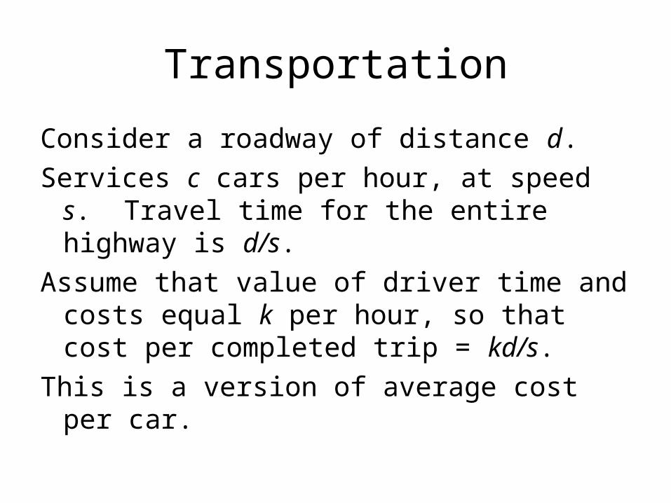
Consider a roadway of distance d.

Services c cars per hour, at speed s. Travel time for the entire highway is d/s.

Assume that value of driver time and costs equal k per hour, so that cost per completed trip = kd/s.

This is a version of average cost per car.

Costs

Cost per completed trip = kd/s

Total cost = c*AC = ckd/s

Marginal cost =

dTC/dc = kd/s - (ckd/s2)(ds/dc)

MC = AC - (ckd/s2)(ds/dc)

AC (1 – Esc), where Esc = Elasticity

Since (ds/dc) 0, we have congestion as c .

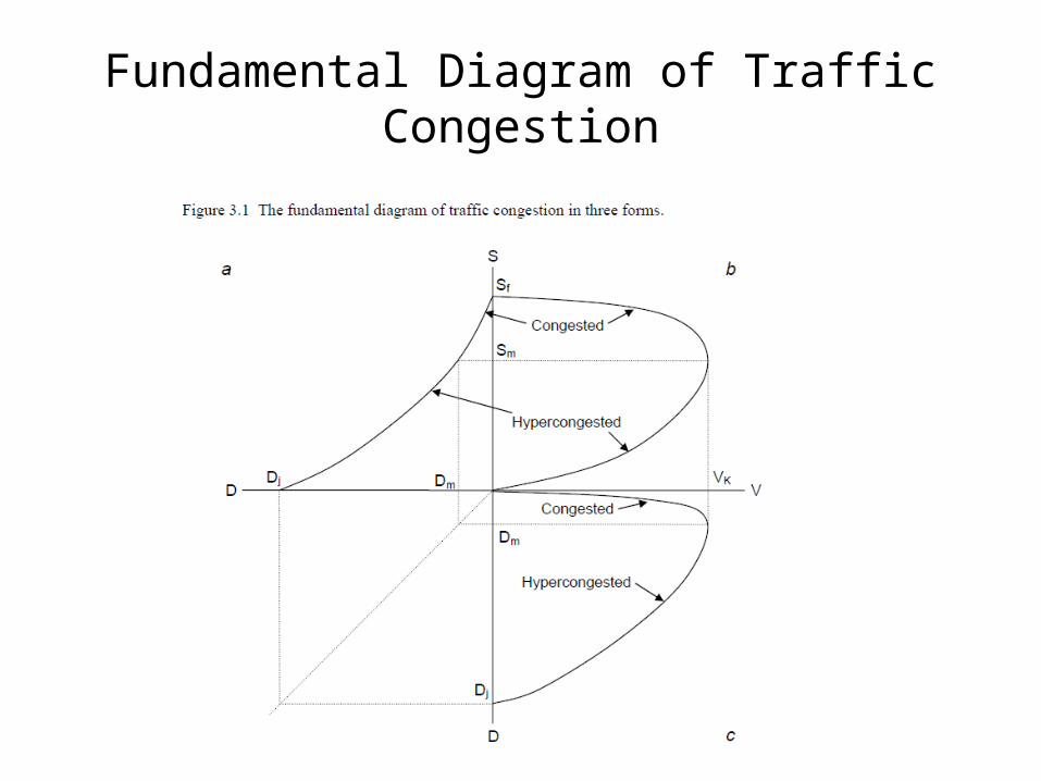
Fundamental Diagram of Traffic Congestion

Costs

MC = AC - (ckd/s2)(ds/dc)

AC (1 – Esc),

c

$ AC

- (AC)(Esc)

Let’s look at demand D.

Optimal toll = MC - AC =

- (ckd/s2)(ds/dc)

= -AC*Esc

D

Toll

Note: In this model, you STILL have congestion, even with the optimal toll..

Economies of Scale

If mc < ac, then s > 1, economies of scale

If mc > ac, then s < 1, diseconomies of scale

In LR, almost everything is variable so you are more likely to have s about equal to 1.

In SR, with fixed capital, more likely to have economies of scale.

/

/

ac C qs

mc C Q

Final and Intermediate Outputs

• Final outputs = quantity and/or extent of trips taken. • Intermediate outputs = vehicle-miles, vehicle-hours,

and peak vehicles in service. • Environment might include

– the length of a corridor,

– the area from which it draws patronage, densities of trip origins and destinations, and

– possible methods by which passengers can access the system and reach their final destinations.

Cost Functions for Public Transit

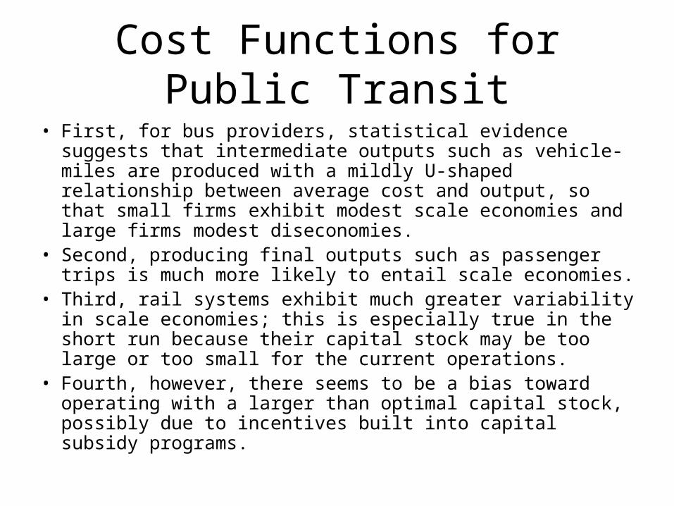
• First, for bus providers, statistical evidence suggests that intermediate outputs such as vehicle-miles are produced with a mildly U-shaped relationship between average cost and output, so that small firms exhibit modest scale economies and large firms modest diseconomies.

• Second, producing final outputs such as passenger trips is much more likely to entail scale economies.

• Third, rail systems exhibit much greater variability in scale economies; this is especially true in the short run because their capital stock may be too large or too small for the current operations.

• Fourth, however, there seems to be a bias toward operating with a larger than optimal capital stock, possibly due to incentives built into capital subsidy programs.

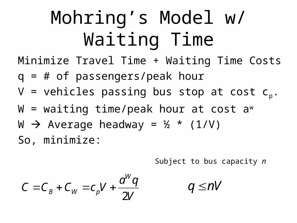
Mohring’s Model w/ Waiting Time

Minimize Travel Time + Waiting Time Costs

q = # of passengers/peak hour

V = vehicles passing bus stop at cost cp.

W = waiting time/peak hour at cost aw

W Average headway = ½ * (1/V)

So, minimize:

2

W

B W p

a qC C C c V

V

Subject to bus capacity n

q nV

Optimizing

• If λ = 0 (buses aren’t full)– Optimal frequency V* is proportional to square root of

passenger density q.– Cost function is also proprtional to q½ .

• If buses ARE full, Over the range of output for which this solution holds, the total cost function is linear in output and has fixed cost CW * .

• It thus again exhibits density economies s=1+(CW * /CB * .), which are greater, the greater are waiting-time costs compared to operating costs

20

2p

aWqc n

V

So

• So whether or not the constraint is binding, there are economies of density because either operating costs or waiting costs grow less than proportionally as output expands.

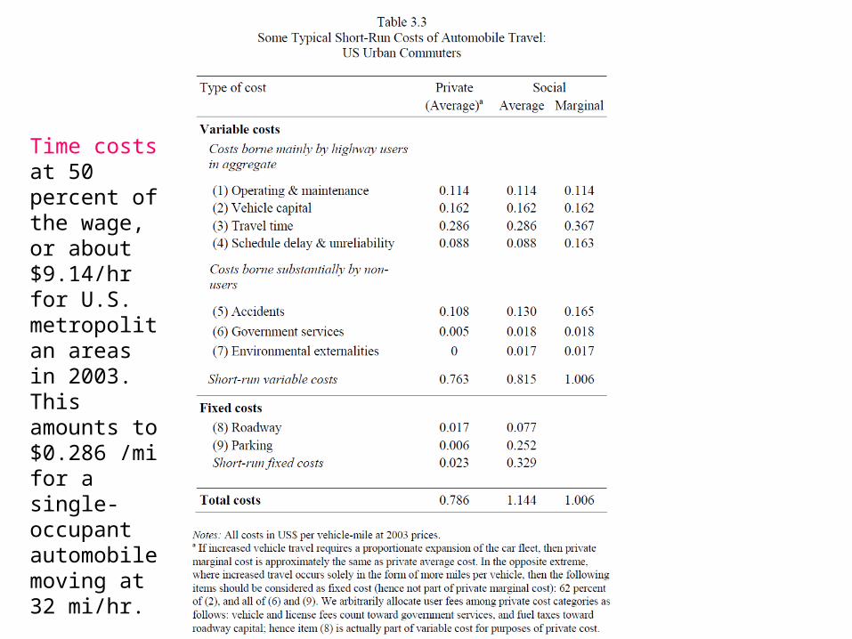
Time costs at 50 percent of the wage, or about $9.14/hr for U.S. metropolitan areas in 2003.This amounts to $0.286 /mi for a single-occupant automobile moving at 32 mi/hr.

Is highway travel subsidized? • Table 3.3 could be used to argue that in the SR, private decision-makers are

“subsidized” at the margin by $0.220 per vehicle-mile if they choose to travel by car.

• Given the capital decisions that have been made with respect to provision of roads and parking spaces, this measures the extent of the distortion in the average incentive facing car users.

• But more striking is that most of this discrepancy arises from the congestion externality, and most of the rest arises from inter-user externalities connected with accidents. These externalities are well understood to vary greatly by circumstance.

• So from an efficiency point of view, the table is most useful by pointing to congestion and accidents as two places to look for big savings from more efficient policies.

• Similarly, looking at long-run policies, we see that parking is supplied at an enormous subsidy to such an extent, in fact, that we deemed the short-run costs of searching for parking spaces too small to bother to quantify for the US.

• So very likely there are big savings to be reaped from policies that reduce provision of parking spaces, especially if some of the fixed costs can be recovered, for example by converting parking lots to other uses or by arranging for existing parking structures to be shared with nearby new users.

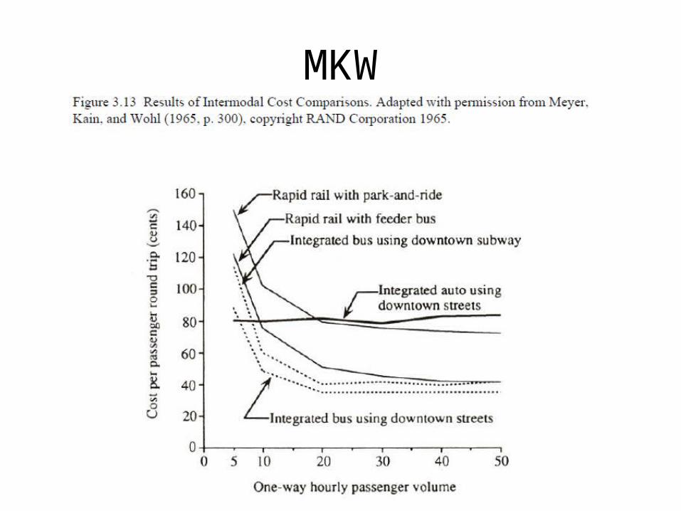
MKW

Three parts of trips

• Collection

• Line haul

• Distribution

• This is true for ALL transportation, passenger or freight.

Intermodal Cost Comparisons

• All results are for a ten-mile limited-access line-haul facility (auto-only expressway, exclusive busway, or rapid-rail line), combined with a two-mile downtown distribution route.

• Bus service is integrated, meaning that collection, line haul, and distribution is all done by a single vehicle.

• Downtown distribution for rail and for one of the bus systems is accomplished using exclusive underground right of way; for the other bus system and for auto, it is accomplished using city streets.

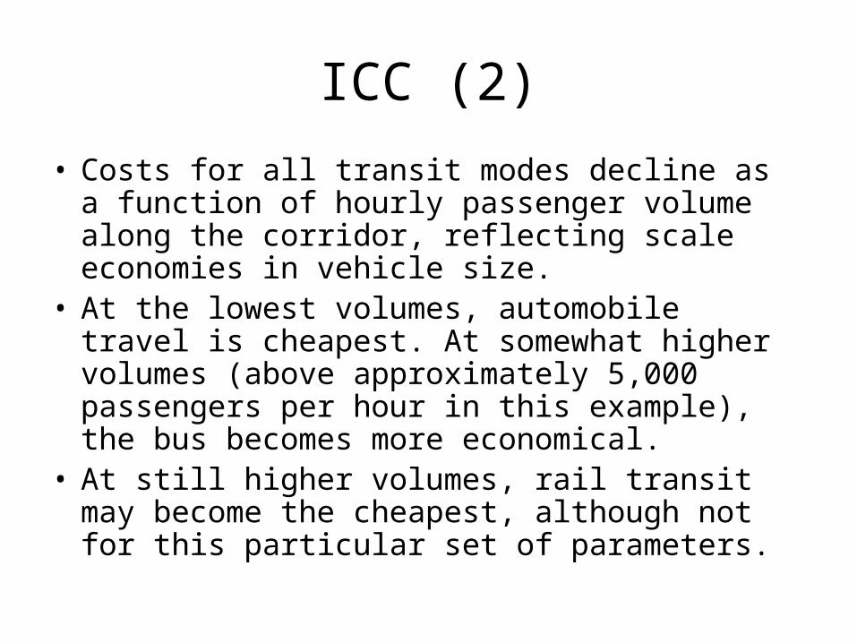
ICC (2)

• Costs for all transit modes decline as a function of hourly passenger volume along the corridor, reflecting scale economies in vehicle size.

• At the lowest volumes, automobile travel is cheapest. At somewhat higher volumes (above approximately 5,000 passengers per hour in this example), the bus becomes more economical.

• At still higher volumes, rail transit may become the cheapest, although not for this particular set of parameters.

Kain (1999) construction costs

Why is rail so costly?The biggest cost factor accounting for these differences is the capital

cost of the infrastructure. Kain (1999) focuses on this item, comparing more recent evidence for four types of express transit in North American cities: rapid rail, light rail, bus on exclusive busway, and bus on shared carpool lanes.

Some of his results are shown in Table 3.5. It is evident that at the ridership levels achieved by these systems, both heavy and light rail are many times more expensive than express bus, even before accounting for their higher operating costs.

Comparisons such as these have led to widespread skepticism among economists toward new rail systems. The evidence is very strong that in all but very dense cities, equivalent transportation can be provided far more cheaply by a good bus system, using exclusive right of way where necessary to bypass congestion.

There is also strong evidence, as noted earlier, that many rail systems in the US have been approved based upon misleading projections of their costs and ability to attract riders.

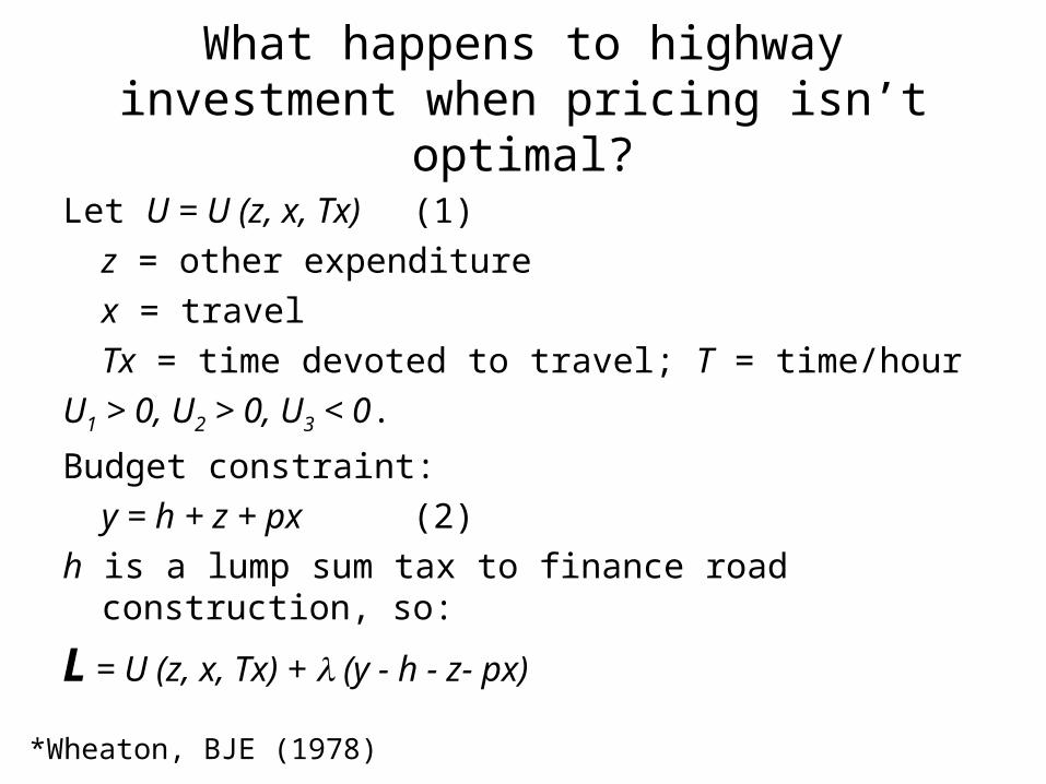
What happens to highway investment when pricing isn’t optimal?

Let U = U (z, x, Tx) (1)

z = other expenditure

x = travel

Tx = time devoted to travel; T = time/hour

U1 > 0, U2 > 0, U3 < 0.

Budget constraint:

y = h + z + px (2)

h is a lump sum tax to finance road construction, so:

L = U (z, x, Tx) + (y - h - z- px)

*Wheaton, BJE (1978)

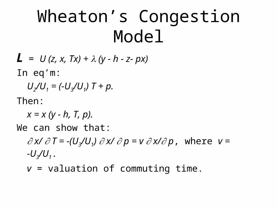
Wheaton’s Congestion Model

L = U (z, x, Tx) + (y - h - z- px)

In eq’m:

U2/U1 = (-U3/U1) T + p.

Then:

x = x (y - h, T, p).

We can show that:

x/ T = -(U3/U1) x/ p = v x/ p, where v = -U3/U1.

v = valuation of commuting time.

Road capacity s travel time function:

T (x, nx) 0

T/ s < 0

2T/ s2 > 0

t/ nx > 0

2T/ (nx)2 > 0.

2T/ nx s < 0.

For congestion, assume that travel time T depends only on ratio of volume nx to capacity s, or T = T (nx/s) = T [n(x/s)]

Yields:

T/ s = -( T/ x) (x/s).

T/( s/s) = -[ T/( x/x) ].

Finally, assume that:

(dx/ds)(s/x) <1. 1% in s less than 1% in travel x.

Society’s optimum?

Optimize:

U{z(h, p, s), x (h, p, s), x(h, p, s) T [s, ns (h, p, s)]} (9)

with respect to s.

Balanced budget constraint:

nh + npx = s (10)

h + px - s/n = 0.

Optimize:

U{z(h, p, s), x (h, p, s), x(h, p, s) T [s, ns (h, p, s)]} (9)

with respect to s.

Balanced budget constraint:

nh + npx = s (10)

h + px - s/n = 0.

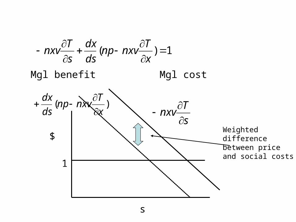
With p given, we get:

-nxv T/ s + (dx/ds) (np - nxv T/ x) = 1.

If we optimize with respect to s and p, we get:

p = xv T/ x -nxv T/ s = 1.

1)(

x

Tnxvnp

ds

dx

s

Tnxv

Mgl benefit Mgl cost

s

$

1

s

Tnxv

)(

x

Tnxvnp

ds

dx

Weighteddifferencebetween priceand social costs

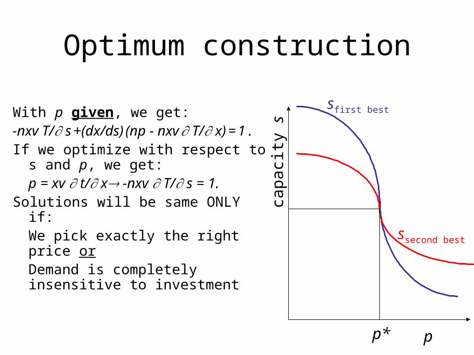
Optimum construction

With p given, we get:-nxv T/ s +(dx/ds) (np - nxv T/ x) = 1.If we optimize with respect to s and p,

we get:p = xv t/ x -nxv T/ s = 1.

Solutions will be same ONLY if:We pick exactly the right price orDemand is completely insensitive to investment

p*

capa

city

s

p

sfirst best

ssecond best

Optimum construction

If p < p*, sf leads to too much s.

ss calls for a relative reduction in investment. This will congestion, “price,” thus demand that has been artificially induced by under-pricing

p*

capa

city

s

p

sfirst best

ssecond best

po

so

We have had user fees but they certainly can’t be characterized as optimal.