Embed Size (px)
Citation preview
Transportation cost-information and concentration
inequalities for bifurcating Markov chains
Simeon Valere Bitseki Penda, Mikael Escobar-Bach, Arnaud Guillin
To cite this version:
Simeon Valere Bitseki Penda, Mikael Escobar-Bach, Arnaud Guillin. Transportation cost-information and concentration inequalities for bifurcating Markov chains. 2015. <hal-01109760>
HAL Id: hal-01109760
https://hal.archives-ouvertes.fr/hal-01109760
Submitted on 26 Jan 2015
HAL is a multi-disciplinary open accessarchive for the deposit and dissemination of sci-entific research documents, whether they are pub-lished or not. The documents may come fromteaching and research institutions in France orabroad, or from public or private research centers.
L’archive ouverte pluridisciplinaire HAL, estdestinee au depot et a la diffusion de documentsscientifiques de niveau recherche, publies ou non,emanant des etablissements d’enseignement et derecherche francais ou etrangers, des laboratoirespublics ou prives.

Transportation cost-information and concentration
inequalities for bifurcating Markov chains
S. Valere Bitseki Penda∗ Mikael Escobar-Bach †
Arnaud Guillin ‡
January 27, 2015
Abstract
We investigate the transportation cost-information inequalities forbifurcating Markov chains which are a class of processes indexed bybinary tree. These processes provide models for cell growth wheneach individual in one generation gives birth to two offsprings in thenext one. Transportation cost inequalities provide useful concentra-tion inequalities. We also study deviation inequalities for the empiri-cal means under relaxed assumptions on the Wasserstein contractionof the Markov kernels. Applications to bifurcating non linear autore-gressive processes are considered: deviation inequalities for pointwiseestimates of the non linear leading functions.
Keywords: Transportation cost-information inequalities, Wasserstein distance, bi-
furcating Markov chains, deviation inequalities, geometric ergodicity.
1 Introduction
Roughly speaking, a bifurcating Markov chain is a Markov chain indexedby a binary regular tree. This class of processes are well adapted for thestudy of populations where each individual in one generation gives birth
∗CMAP, Ecole polytechnique route de Saclay, 91128, Palaiseau, France. email: bit-
[email protected]†Department of Mathematics and Computer Science, University of Southern Denmark,
Campus 55, 5230 Odense M, Denmark email:[email protected]‡Institut Universitaire de France et Laboratoire de Mathematiques, CNRS UMR 6620,
Universite Blaise Pascal, 24 avenue des Landais, BP 80026, 63177 Aubiere, France. email:
1

to two offsprings in the next one. They were introduced by Guyon [29]in order to study the Escherichia coli aging process. Namely, when a celldivides into two offsprings, are the genetical traits identical for the twodaughter cells? Recently, several models of bifurcating Markov chains, ormodels using the theory of bifurcating Markov chains, for example underthe form of bifurcating autoregressive processes, have been studied [1, 2, 29,21, 18], showing that these processes are of great importance to analysisof cell division. There is now an important literature covering asymptotictheorems for bifurcating Markov chains such as Law of Large Numbers,Central Limit Theorems, Moderate Deviation Principle, Law of IteratedLogarithm, see for example [29, 30, 6, 19, 15, 18, 8] for recent references.These limit theorems are particularly useful when applied to the statisticsof the bifurcating processes, enabling to provide efficient tests to assert ifthe aging of the cell is different for the two offsprings (see [30] for realcase study). Of course, these limit theorems may be considered only in the”ergodic” case, i.e. when the law of the random lineage chain has an uniqueinvariant measure.
However, limit theorems are only asymptotical results and one is oftenfaced to study only datas with a size limited population. It is thus verynatural to control the statistics non asymptotically. Such deviation inequal-ities (or concentration inequalities) have been recently the subject of manystudies and we refer to the books of Ledoux [31] and Massart [35] for niceintroductions on the subject, developing both i.i.d. case and dependentcase with a wide variety of tools (Laplace controls, functional inequalities,Efron-Stein,...). It was one of the goal of Bitseki et al. [8] to investigatedeviation inequalities for additive functionals of bifurcating Markov chain.In their work, one of the main hypothesis is that the Markov chain as-sociated to a random lineage of the population is uniformly geometricallyergodic. It is clearly a very strong assumption, nearly reducing interestingmodels to the compact case. The purpose of this paper is to considerablyweaken this hypothesis. More specifically, our aim is to obtain deviationinequalities for bifurcating Markov chain when the auxiliary Markov chainsmay satisfy some contraction properties in Wasserstein distance, and some(uniform) integrabilty property. This will be done with the help of trans-portation cost-information inequalities and direct Laplace controls. In orderto present our result, we may now define properly the model of bifurcatingMarkov chains.
2

1.1 Bifurcating Markov chains
First we introduce some useful notations. Let T be a regular binary tree inwhich each vertex is seen as a positive integer different from 0. For r ∈ N,let
Gr =2r, 2r + 1, · · · , 2r+1 − 1
, Tr =
r⋃
q=0
Gq,
which denote respectively the r-th column and the first (r + 1) columns ofthe tree. The whole tree is thus defined by
T =
∞⋃
r=0
Gr.
A column of a given vertex n is Grn with rn = ⌊log2 n⌋, where ⌊x⌋ denotesthe integer part of the real number x.
In the sequel, we will see T as a given population in which each individualin one generation gives birth to two offsprings in the next one. This will makeeasier the introduction of different notions. The vertex n will denote theindividual n and the ancestor of individuals 2n and 2n+1. The individualswho belong to 2N (resp. 2N+1) will be called individual of type 0 (resp. type1). The column Gr and the first (r+1) columns Tr will denote respectivelythe r-th generation and the first (r + 1) generations. The initial individualwill be denoted 1.
For each individual n, we look into a random variable Xn, defined ona probability space (Ω,F ,P) and which takes its values in a metric space(E, d) endowed with its Borel σ-algebra E . We assume that each pair ofrandom variables (X2n,X2n+1) depends of the past values (Xm,m ∈ Trn)only through Xn. In order to describe this dependance, let us introduce thefollowing notion.
Definition 1.1 (T-transition probability, see ([29])). We call T-transitionprobability any mapping P : E × E2 → [0, 1] such that
• P (·, A) is measurable for all A ∈ E2,
• P (x, ·) is a probability measure on (E2, E2) for all x ∈ E.
In particular, for all x, y, z ∈ E, P (x, dy, dz) denotes the probabilitythat the couple of the quantities associated with the children are in theneighbourhood of y and z given that the quantity associated with theirmother is x.
3

For a T-transition probability P on E×E2, we denote by P0, P1 the firstand the second marginal of P , that is P0(x,A) = P (x,A × E), P1(x,A) =P (x,E × A) for all x ∈ E and A ∈ E . Then, P0 (resp. P1) can be seen asthe transition probability associated to individual of type 0 (resp. type 1).
For p ≥ 1, we denote by B(Ep) (resp. Bb(Ep)), the set of all Ep-
measurable (resp. Ep-measurable and bounded) mappings f : Ep → R.For f ∈ B(E3), we denote by Pf ∈ B(E) the function
x 7→ Pf(x) =
∫
S2
f(x, y, z)P (x, dy, dz), when it is defined.
We are now in position to give a precise definition of bifurcating Markovchain.
Definition 1.2 (Bifurcating Markov Chains, see ([29])). Let (Xn, n ∈ T)be a family of E-valued random variables defined on a filtered probabilityspace (Ω,F , (Fr, r ∈ N),P). Let ν be a probability on (E, E) and P be a T-transition probability. We say that (Xn, n ∈ T) is a (Fr)-bifurcating Markovchain with initial distribution ν and T-transition probability P if
• Xn is Frn-measurable for all n ∈ T,
• L(X1) = ν,
• for all r ∈ N and for all family (fn, n ∈ Gr) ⊆ Bb(E3)
E
[∏
n∈Gr
fn(Xn,X2n,X2n+1)∣∣∣Fr
]=∏
n∈Gr
Pfn(Xn).
In the following, when unprecised, the filtration implicitly used will beFr = σ(Xi, i ∈ Tr).
Remark 1.3. We may of course also consider in this work bifurcating Markovchains on a a-ary tree (with a ≥ 2) with no additional technicalities, butheavy additional notations. In the same spirit, Markov chains of higherorder (such as BAR processes considered in [7]) could be handled by thesame techniques. A non trivial extension would be the case of bifurcatingMarkov chains on a Galton-Watson tree (see for example [10] under verystrong assumptions), that we will consider elsewhere.
4
1.2 Transportation cost-information inequality
We recall that (E, d) is a metric space endowed with its Borel σ-algebra E .Given p ≥ 1, the Lp-Wasserstein distance between two probability measuresµ and ν on E is defined by
W dp (ν, µ) = inf
(∫ ∫d(x, y)pdπ(x, y)
)1/p
,
where the infimum is taken over all probability measures π on the productspace E × E with marginal distributions µ and ν (say, coupling of (µ, ν)).This infimum is finite as soon as µ and ν have finite moments of order p.When d(x, y) = 1x 6=y (the trivial measure), 2W d
1 (µ, ν) = ‖µ − ν‖TV , thetotal variation of µ− ν.
The Kullback information (or relative entropy) of ν with respect to µ isdefined as
H(ν/µ) =
∫log dν
dµdν, if ν ≪ µ
+∞ else.
Definition 1.4 (Lp-transportation cost-inequality). We say that the prob-ability measure µ satisfies the Lp-transportation cost-information inequalityon (E, d) (and we write µ ∈ Tp(C)) if there is some constant C > 0 suchthat for any probability measure ν,
W dp (µ, ν) ≤
√2CH(ν/µ).
This transportation inequality have been introduced by Marton [32, 33]as a tool for (Gaussian) concentration of measure property. The follow-ing result will be crucial in the sequel. It gives a characterization of L1-transportation cost-inequality in term of concentration inequality. It is ofcourse one of the main tool to get deviation inequalities (via Markov in-equality).
Theorem 1.5 ([11]). µ satisfies the L1-transportation cost-information in-equality (say T1) on (E, d) with constant C > 0, that is, µ ∈ T1(C), if andonly if for any Lipschitzian function F : (E, d) → R, F is µ-integrable and
∫
Eexp (λ (F − 〈F 〉µ)) dµ ≤ exp
(λ2
2C‖F‖2Lip
)∀λ ∈ R,
where 〈F 〉µ =∫E Fdµ and
‖F‖Lip = supx 6=y
|F (x)− F (y)|d(x, y)
< +∞.
5

In particular, we have the concentration inequality
µ (F − 〈F 〉µ ≤ −t) ∨ µ (F − 〈F 〉µ ≥ t) ≤ exp
(− t2
2C‖F‖2Lip
)∀t ∈ R.
In this work we will focus on transportation inequality T1 mainly. Thereis now a considerable literature around these transportation inequalities. Asa flavor, let us cite first the characterization of T1 as a Gaussian integrabilityproperty [20] (see also [23]).
Theorem 1.6 ([20]). µ satisfies the L1-transportation cost-information in-equality (say T1) on (E, d) if and only if there exists δ > 0 and x0 ∈ E suchthat
µ(eδd
2(x,x0))< ∞,
and the constant of the Transportation inequality can be made explicit.
There is also a large deviations characterization [25]. Recent strikingresults on transportation inequalities have been obtained for T2, namelythat they are equivalent to dimension free Gaussian concentration [24], orto a restricted class of logarithmic Sobolev inequalities [27]. Se also [13] or[14] for practical criterion based on Lyapunov type criterion and we refer forexample to [26] or [37] for surveys on transportation inequality. One of themain aspect of transportation inequality is their tensorization property, i.e.µ⊗n will satisfy some transportation measure if µ does (with dependence onthe dimension n2/p−1) . One important development was to consider such aproperty for dependent sequences such as Markov chains. In [20], Djellout etal., generalizing result of Marton [34], have provided conditions under whichthe law of a homogeneous Markov chain (Yk)1≤k≤n on En satisfies the Lp-transportation cost-information inequality Tp with respect to the metric
dlp(x, y) :=
(n∑
i=1
d(xi, yi)p
)1/p
.
We will follow similar ideas here to establish the Lp- transportation cost-information inequality for the law of a bifurcating Markov chain (Xi)1≤i≤N
on EN . This will allow us to obtain concentration inequalities for bifurcat-ing Markov chains under hypotheses largely weaker than those of Bitsekiet al. [8]. It would also be tempting to generalize the approach of [28] toMarkov chains and bifurcating Markov chains to get directly deviation in-equalities for Markov chains, w.r.t. the invariant measure. However it wouldneed to restrict to reversible Markov chains and thus not directly suited tobifurcating Markov chains and would thus recquire new ideas.
6

Remark 1.7. There are natural generalizations of the T1 inequality oftendenoted α − T1 inequality, where α is a non negative convex lower semicontinuous function vanishing at 0. We say that the probability measure µsatisfies α− Tp(C) if for any probability measure ν
α (W1(ν, µ)) ≤ 2C H(ν/µ).
The usual T1 inequality is then the case where α(t) = t2. Gozlan [23]has generalized Bobkov-Gotze’s Laplace transform control [11] and Djellout-Guillin-Wu [20] integrability criterion to this setting enabling to recover subor super Gaussian concentration. The result of the following section canbe generalized to this setting, however adding technical details and heavynotations. Details will thus be left to the reader.
2 Transportation cost-information inequalities for
bifurcating Markov chains
Let (Xi, i ∈ T) be a bifurcating Markov chain on E with T-probabilitytransition P and initial measure ν. For p ≥ 1 and C > 0, we consider thefollowing assumption that we shall call (Hp(C)) in the sequel.
Assumption 2.1 (Hp(C)).
(a) ν ∈ Tp(C);
(b) P (x, ·, ·) ∈ Tp(C), ∀x ∈ E ;
(c) W dp (P (x, ·, ·), P (x, ·, ·)) ≤ q d(x, x), ∀x, x ∈ E and some q > 0.
It is important to remark that under (Hp(C)), (c) we have that thereexists r0 and r1 smaller than q such that for b = 0, 1
W dp (Pb(x, ·), Pb(x, ·)) ≤ rb d(x, x), ∀x, x ∈ E.
Note also that when P (x, dy, dz) = P0(x, dy)P1(x, dz), then these last twostability results in Wasserstein contraction implies (Hp(C)), (c) with q ≤(rp0+rp1)
1/p (using trivial coupling). We may remark also that by (Hp(C)), (b),P0 and P1 also satisfies (uniformly) a transportation inequality. Let us notethat thanks to the Holder inequality, (Hp(C)) implies (H1(C)).We do not suppose here that q, r0 and r1 are strictly less than 1, and thusthe two marginal chains, as well as the bifurcating one, are not a priori
7

contractions. We are thus considering here both ”stable” and ”unstable”cases.
We then have the following result for the law of the whole trajectory onthe binary tree.
Theorem 2.2. Let n ∈ N and let P be the law of (Xi)1≤i≤Tn and denoteN = |Tn|. We assume Assumption 2.1 for 1 ≤ p ≤ 2. Then P ∈ Tp (CN )where
CN =
CN2/p−1
(1−q)2if q < 1
C exp(2− 2
p
)N2/p+1 if q = 1
C (N + 1)(exp(q−1)rpN
rp−1
)2/pif q > 1.
Before the proof of this result, let us make the following notations. For aPolish space χ, we denote by M1(χ) the space of probability measures on χ.For x ∈ EN , xi := (x1, · · · , xi). For µ ∈ M1(E
N ), let (x1, · · · , xN ) ∈ EN bedistributed randomly according to µ. We denote by µi the law of x2i+1, andby µi
x2i−1 the conditional law of (x2i, x2i+1) given x2i−1 with the conventionµ1x0 = µ1, where x0 = x0 is some fixed point. In particular, if µ is the
law of a bifurcating Markov chain with T-probability transition P , thenµix2i−1 = P (xi, ·, ·).For the convenience of the readers, we recall the formula of additivity of
entropy (see for e.g. [37], Lemma 22.8).
Lemma 2.3. Let N ∈ N, let χ1, · · · , χN be Polish spaces and P,Q ∈ M1(χ)where χ =
∏Ni=1 χi. Then
H(Q|P) =
N∑
i=1
∫
χH(Qi
xi−1 |Pixi−1)Q(dx)
where Pixi−1 and Qi
xi−1 are defined in the same way as above.
We can now prove the Theorem.
Proof of the Theorem 2.2. Let Q ∈ M1(EN ). Assume that H(Q|P) < ∞
(trivial otherwise). Let ε > 0. The idea is of course to do a conditionnementwith respect to the previous generation, i.e. to Gn−1 but we will do itsequentially by pairs. Conditionally to their ancestors, every pair of offspringof an individual is independent of the offspring of the other individuals forthe same generation. Let i be a member of generation Gj−1, and define fora realization x on the tree Ti(x) := (x1, ..., x|Tj |). By the definition of the
8

Wasserstein distance, there is a coupling πiy2i−1,x2i−1 of (Qi
y2i−1 ,Pix2i−1) such
that
Ai :=
∫(d(y2i, x2i)
p + d(y2i+1, x2i+1)p)dπi
y2i−1,x2i−1
≤ (1 + ǫ)W dp
(Qi
y2i−1 ,Pix2i−1
)p
≤ (1 + ǫ)[W d
p
(Qi
y2i−1 ,Piy2i−1
)+W d
p
(Piy2i−1 ,Pi
x2i−1
)]p
≤ (1 + ǫ)[W d
p
(Qi
y2i−1 , P (yi, ·, ·))+W d
p
(P (yi, ·, ·) , P (xi, ·, ·)
)]p,
where the second inequality is obtained thanks to the triangle inequality forthe W d
p distance and the equality is a consequence of the Markov property.By Assumption 2.1, and the convexity of the function x 7→ xp, we obtain,for a, b > 1 such that 1/a+ 1/b = 1,
Ai ≤ (1 + ǫ)
(√2CHi(y2i−1) + qd(yi, xi)
)p
≤ (1 + ǫ)
(ap−1
(√2CHi(y2i−1)
)p
+ bp−1qpdp(yi, xi)
)
where Hi(y2i−1) = H(Qi
y2i−1 |Piy2i−1). By recurrence, it leads to the finite-
ness of p-moments. Taking the average with respect to the whole law andsumming on i, we obtain
|Tn−1|∑
i=0
E(Ai)
≤ (1 + ε)
ap−1 (2C)p/2
|Tn−1|∑
i=1
E
[Hi(Y
2i−1)p/2]+
bp−1qp
|Tn−2|∑
i=0
E(Ai)
.
Letting ε goes to 0+, we are led to
|Tn−1|∑
i=0
E(Ai)
≤N∑
i=1
(ap−1 (2C)p/2 E
[Hi(Y
i−1)p/2])
+
bp−1qp
|Tn−2|∑
i=0
E(Ai)
.
9
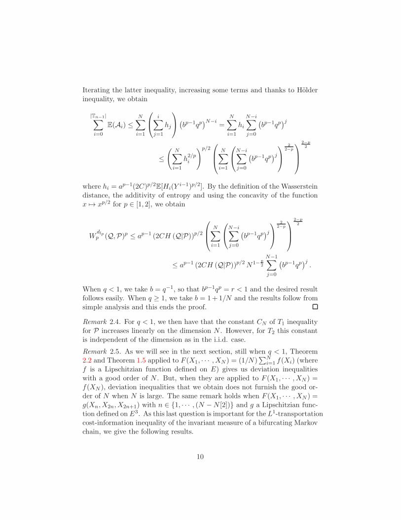
Iterating the latter inequality, increasing some terms and thanks to Holderinequality, we obtain
|Tn−1|∑
i=0
E(Ai) ≤N∑
i=1
i∑
j=1
hj
(bp−1qp
)N−i=
N∑
i=1
hi
N−i∑
j=0
(bp−1qp
)j
≤(
N∑
i=1
h2/pi
)p/2
N∑
i=1
N−i∑
j=0
(bp−1qp
)j
2
2−p
2−p2
where hi = ap−1(2C)p/2E[Hi(Yi−1)p/2]. By the definition of the Wasserstein
distance, the additivity of entropy and using the concavity of the functionx 7→ xp/2 for p ∈ [1, 2], we obtain
Wdlpp (Q,P)p ≤ ap−1 (2CH (Q|P))p/2
N∑
i=1
N−i∑
j=0
(bp−1qp
)j
2
2−p
2−p2
≤ ap−1 (2CH (Q|P))p/2 N1− p2
N−1∑
j=0
(bp−1qp
)j.
When q < 1, we take b = q−1, so that bp−1qp = r < 1 and the desired resultfollows easily. When q ≥ 1, we take b = 1+1/N and the results follow fromsimple analysis and this ends the proof.
Remark 2.4. For q < 1, we then have that the constant CN of T1 inequalityfor P increases linearly on the dimension N . However, for T2 this constantis independent of the dimension as in the i.i.d. case.
Remark 2.5. As we will see in the next section, still when q < 1, Theorem2.2 and Theorem 1.5 applied to F (X1, · · · ,XN ) = (1/N)
∑Ni=1 f(Xi) (where
f is a Lipschitzian function defined on E) gives us deviation inequalitieswith a good order of N . But, when they are applied to F (X1, · · · ,XN ) =f(XN ), deviation inequalities that we obtain does not furnish the good or-der of N when N is large. The same remark holds when F (X1, · · · ,XN ) =g(Xn,X2n,X2n+1) with n ∈ 1, · · · , (N −N [2]) and g a Lipschitzian func-tion defined on E3. As this last question is important for the L1-transportationcost-information inequality of the invariant measure of a bifurcating Markovchain, we give the following results.
10

Proposition 2.6. Under (H1(C)), for any n ∈ T and x ∈ E
L(Xn|X1 = x) ∈ T1(cn)
where
cn = C
rn−1∑
k=0
r2(k−ak)0 r2ak1 ; a0 = 0
and for all k ∈ 1, · · · , rn− 1, ak is the number of ancestor of type 1 of Xn
which are between the rn − k + 1-th generation and the rn-th generation.
Before the proof, we introduce some more notations. Let n ∈ T. Wedenote by (z1, · · · , zrn) ∈ 0, 1rn the unique path from the root 1 to n.Then, for all i ∈ 1, · · · , rn, zi is the type of the ancestor of n which is inthe i-th generation and the quantities ak defined in the Proposition 2.6 aregiven by
ak =
rn∑
i=rn−k+1
zi.
For all k ∈ 1, · · · , rn, we denote by P k and P−k the iterated of the tran-sition probabilities P0 and P1 defined by
P k := Pz1 · · · Pzk and P−k := Pzrn−k · · · Pzrn .
Proof of the Proposition 2.6. First note that since
W d1 (ν, µ) = sup
f :‖f‖Lip≤1
∣∣∣∣∫
Sfdµ−
∫
Sfdν
∣∣∣∣ ,
condition (c) of (H1(C)) implies that
‖Pbf‖Lip ≤ rb‖f‖Lip ∀b ∈ 0, 1.
Now let f be a Lipschitzian function defined on E. By (b)-(c) of (H1(C))and Theorem 1.5, we have
P rn(ef ) ≤ P rn−1
(exp
(Prnf +
C‖f‖2Lip2
)).
Once again, applying Theorem 1.5, we obtain
P rn(ef ) ≤ P rn−2
(exp
(P−1f +
C‖f‖2Lip2
+C‖Pzrnf‖2Lip
2
)).
11

By iterating this method, we are led to
P rn(ef ) ≤ exp
(P−rn+1f + (1 + r2zrn + r2zrnr
2zrn−1
+ · · · +rn∏
i=2
r2zi)C‖f‖2Lip
2
).
Since
1+r2zrn+r2zrnr2zrn−1
+· · ·+rn∏
i=2
r2zi =
rn−1∑
k=0
r2(k−ak)0 r2ak1 and P−rn+1f = P rnf,
we conclude the proof thanks to Theorem 1.5.
The next result is a consequence of the previous Proposition.
Corollary 2.7. Assume (H1(C)) and r := maxr0, r1 < 1. Then
L(Xn|X1 = x) ∈ T1(c∞) and L((Xn,X2n,X2n+1)|X1 = x) ∈ T1(c′∞)
where
c∞ =C
1− r2and c′∞ = C
(1 +
(1 + q)2
1− r2
).
Proof. That L(Xn|X1 = x) ∈ T1(c∞) is a direct consequence of Proposition2.6. It suffices to bound r0 and r1 by r.
In order to deal with the ancestor-offspring case (Xn,X2n,X2n+1), wedo the following remarks.
Let f : (E3, dl1) → R be a Lipschitzian function. We have
‖Pf‖Lip = supx,x∈E
∣∣∫ f(x, y, z)P (x, dy, dz) −∫f(x, y, z)P (x, dy, dz)
∣∣d(x, x)
.
Thanks to condition (c) of (H1(C)), we have the following inequalities∣∣∣∣∫
f(x, y, z)P (x, dy, dz) −∫
f(x, y, z)P (x, dy, dz)
∣∣∣∣
≤ ‖f‖Lip(d(x, x) +W
dl11 (P (x, ·), P (x, ·))
)
≤ (q + 1)‖f‖Lipd(x, x),
and then,‖Pf‖Lip ≤ (q + 1)‖f‖Lip.
We recall that X1 = x. We have
E [exp (f(Xn,X2n,X2n+1))] = P rn(Pef (x)).
12

Now, from (H1(C)), the previous remarks and using the same strategy asin the proof of Proposition 2.6, we are led to
E [exp (f(Xn,X2n,X2n+1))]
≤ exp
(Pz1 · · ·PzrnPf(x) +
C‖f‖2Lip2
+C(1 + q)2‖f‖2Lip
2
rn−1∑
i=0
r2i
).
Since Pz1 · · ·PzrnPf(x) = E [f(Xn,X2n,X2n+1)] and∑rn−1
i=0 r2i ≤ 1/(1−r2),we obtain
E [exp (f(Xn,X2n,X2n+1))] ≤ exp(E [f(Xn,X2n,X2n+1)] + c′∞
)
with c′∞ given in the Corollary. We then conclude the proof thanks toTheorem 1.5.
3 Concentration inequalities for bifurcating Markov
chains
3.1 Direct applications of the Theorem 2.2
We are now interested in the concentration inequalities for the additivefunctionals of bifurcating Markov chains. Specifically, let N ∈ N
∗ and I bea subset of 1, · · · , N. Let f be a real function on E or E3. We set
MI(f) =∑
i∈I
f(∆i)
where ∆i = Xi if f is defined on E and ∆i = (Xi,X2i,X2i+1) if f isdefined on E3. We also consider the empirical mean M I(f) over I definedby M I(f) = (1/|I|)MI (f) where |I| denotes the cardinality of I. In thestatistical applications, the cases N = |Tn| and I = Gm (for m ∈ 0, · · · , n)or I = Tn are relevant (see for e.g. [8]).
First, we will establish concentration inequalities when f is a real Lip-schitzian function defined on E. For a subset I of 1, · · · , N, let FI bethe function defined on (EN , dlp), p ≥ 1 by FI(x
N ) = 1/(|I|)∑i∈I f(xi) forall xN ∈ EN . Then FI is also a Lipschitzian function on (EN , dlp) and we
have ‖FI‖Lip ≤ |I|−1/p‖f‖Lip. The following result is a direct consequenceof Theorem 2.2.
13

Proposition 3.1. Let N ∈ N∗ and let P be the law of (Xi)1≤i≤N . Let f be
a real Lipschitzian function on (E, d). Then, under (Hp(C)) for 1 ≤ p ≤ 2,
P F−1I ∈ Tp(CN |I|−2/p‖f‖2Lip)
where CN is given in the Theorem 2.2 and P F−1I is the image law of P
under FI . In particular, for all t > 0 we have
P(FI(X
N ) ≤ −t+ E[FI(X
N )])
∨ P(FI(X
N ) ≥ t+ E[FI(X
N )])
≤ exp
(− t2|I|2/p2CN‖f‖2Lip
).
Proof. The first part is a direct consequence of Theorem 2.2 and Lemma 2.1of [20]. The second part is an application of Theorem 1.5.
For the next concentration inequality, we assume that f is a real Lips-chitzian function defined on (E3, dl1), which means that
|f(x)− f(y)| ≤ ‖f‖Lip3∑
i=1
d(xi, yi) ∀x, y ∈ E3.
We assume that N is a odd number. Let I be a subset of 1, · · · , (N −1)/2. Now, we denote by FI the real function defined on (EN , dlp) byFI(x
N ) = (1/|I|)∑i∈I f(xi, x2i, x2i+1). For all xN , yN ∈ EN we have forsome universal constant c
|FI(xN )− FI(y
N )| ≤ ‖f‖Lip|I|
∑
i∈I
(d(xi, yi) + d(x2i, y2i) + d(x2i+1, y2i+1))
≤ c‖f‖Lip|I|1/p dlp(x
N , yN ).
FI is then a Lipschitzian function on (EN , dlp) and ‖FI‖Lip ≤ c‖f‖Lip/|I|1/p.We then have the following result.
Proposition 3.2. Let N ∈ N∗ be a odd number and let P be the law of
(Xi)1≤i≤N . Let f be a real Lipschitzian function on (E3, dl1). Then, under(Hp(C)) for 1 ≤ p ≤ 2,
P F−1I ∈ Tp(cCN |I|−2/p‖f‖2Lip)
14

where CN is given in the Theorem 2.2 and P F−1I is the image law of P
under FI . In particular, for all t > 0 we have
P(FI(X
N ) ≤ −t+ E[FI(X
N )])
∨ P(FI(X
N ) ≥ t+ E[FI(X
N )])
≤ exp
(− t2|I|2/p2cCN‖f‖2Lip
).
Proof. The proof is a direct consequence of Theorem 2.2, Lemma 2.1 of [20]and Theorem 1.5.
Remark 3.3. The previous results applyed with p = 1 to the empirical meansMGn(f) and MTn(f) (f being a real Lipschitzian function) give us relevantconcentration inequalities, that is with the good order size of the index set,when q < 1. For example, for MGn(f) , it suffices to take N = |Tn| andI = Gn in the Propositions 3.1 and 3.2. But for q ≥ 1, the concentrationinequalities obtained thanks to these results are not satisfactory. In thesequel, we will be interested in obtaining relevant concentration inequalitiesfor the empirical means MGn(f) and MTn(f) when q ≥ 1.
3.2 Gaussian concentration inequalities for the empirical means
MGn(f) and MTn(f)
Throughout this section, we will focus only in the case p = 1, and willassume (H1(C)). We set r = r0 + r1.
The main goal of this subsection is to broaden the range of application ofdeviation inequalities of MGn(f) and MTn(f) to cases where r > 1, namelywhen it is possible that one of the two marginal Markov chains is not astrict contraction. The transportation inequality of Theorem 2.2 is a verypowerful tool to get deviation inequalities for all lipschitzian functions of thewhole trajectory (up to generation n), and may thus concern for exampleLipschitzian function of only offspring generated by P0 or P1. Consequently,to get ”consistent” deviation inequalities, both marginal Markov chains haveto be contractions in Wasserstein distance.However when dealing with MGn(f) or MTn(f), we may hope for an av-eraging effect, i.e. if one is not a contraction and the other one a strongcontraction it may in a sense compensate. Such averaging effect have beenobserved at the level of the LLN and CLT in [29, 16] but only asymptoti-cally. Our purpose here will be then to show that such averaging effect will
15

also affect deviation inequalities.
We will use, directly inspired by Bobkov-Gotze’s Laplace transform con-trol, what we call Gaussian Concentration property: for κ > 0, we will saythat a random variable X satisfies GC(κ) if
E [exp (t (X − E [X]))] ≤ exp(κt2/2
)∀t ∈ R.
Using Markov’s inequality and optimization, this Gaussian concentrationproperty immediately implies that
P(X − E(X) ≥ r) ≤ e−r2
2κ .
We may thus focus here only on the Gaussian concentration property (GC).
Proposition 3.4. Let f be a real Lipschitzian function on E and n ∈ N.Assume that (H1(C)) holds. Then MGn(f) satisfies GC(γn) where
γn =
2C‖f‖2Lip
|Gn|
(1−(r2/2)
n+1
1−r2/2
)if r 6=
√2
2C‖f‖2Lip(n+1)
|Gn|if r =
√2.
We recall that here r = r0 + r1.
Remark 3.5. One can observe that for r <√2, the previous inequalities are
on the same order of magnitude that the inequalities obtained thanks toProposition 3.1 with q < 1. For r < 2 the above inequalities remain relevantsince we just have a negligible loss with respect to |Gn|. But for r ≥
√2,
these inequalities are not significant (see the same type of limitations at theCLT level in [16]).
Proof. Let f be a real Lipschitzian function on E, n ∈ N and t ∈ R. Wehave
E
[exp
(t2−n
∑
i∈Gn
f(Xi)
)]= E
exp
t2−n
∑
i∈Gn−1
(P0 + P1)f(Xi)
×E
exp
t2−n
∑
i∈Gn−1
(f(X2i) + f(X2i+1)− (P0 + P1)f(Xi))
∣∣∣Fn−1
.
16

Thanks to the Markov property, we have
E
exp
t2−n
∑
i∈Gn−1
(f(X2i) + f(X2i+1)− (P0 + P1)f(Xi))
∣∣∣Fn−1
=∏
i∈Gn−1
P(exp
(t2−n (f ⊕ f − (P0 + P1)f)
))(Xi)
where f ⊕ f is the function on E2 defined by f ⊕ f(x, y) = f(x) + f(y).We recall that from (H1(C)) we have P (x, ·, ·) ∈ T1(C) for all x ∈ E. Now,thanks to Theorem 1.5, we have
∏
i∈Gn−1
P(exp
(t2−n (f ⊕ f − (P0 + P1)f)
))(Xi)
≤∏
i∈Gn−1
exp
(t2C‖f ⊕ f‖2Lip
2× 22n
).
Since ‖f ⊕ f‖Lip ≤ 2‖f‖Lip, we are led to
E
[exp
(t2−n
∑
i∈Gn
f(Xi)
)]≤ exp
(22t22n−1C‖f‖2Lip
2× 22n
)
× E
exp
t2−n
∑
i∈Gn−1
(P0 + P1)f(Xi)
.
Doing the same for E[exp(t2−n∑
i∈Gn−1(P0 + P1)f(Xi))] with (P0 + P1)f
replacing f and using the inequality
‖(P0 + P1)f ⊕ (P0 + P1)f‖Lip ≤ 2r‖f‖Lip,
we are led to
E
[exp
(t2−n
∑
i∈Gn
f(Xi)
)]≤ E
exp
t2−n
∑
i∈Gn−2
(P0 + P1)2f(Xi)
× exp
(22t2C‖f‖2Lip2n−1
2× 22n
)exp
(22t2C‖f‖2Lipr22n−2
2× 22n
).
Iterating this method and using the inequalities
‖(P0 + P1)kf ⊕ (P0 + P1)
kf‖Lip ≤ 2rk‖f‖Lip ∀k ∈ 1, · · · , n− 1,
17

we obtain
E
[exp
(t2−n
∑
i∈Gn
f(Xi)
)]≤ exp
(22t2C‖f‖2Lip
2× 22n
n−1∑
k=0
r2k2n−k−1
)
× E[exp
(t2−n(P0 + P1)
nf(X1))]
.
Since E [t2−n(P0 + P1)nf(X1)] = E
[t2−n
∑i∈Gn
f(Xi)]= t2−nν(P0+P1)
nf ,we obtain
E
[exp
(t2−n
(∑
i∈Gn
f(Xi)− ν(P0 + P1)nf
))]
≤ exp
(22t2C‖f‖2Lip
2× 22n
n−1∑
k=0
r2k2n−k−1
)
× E[exp
(t2−n ((P0 + P1)
nf(X1))− ν(P0 + P1)nf)]
.
Thanks to (H1(C)), we conclude that
E
[exp
(t2−n
(∑
i∈Gn
f(Xi)− ν(P0 + P1)nf
))]
≤ exp
(22t2C‖f‖2Lip
2× 22n
n∑
k=0
r2k2n−k−1
)
and the results of the Proposition then follow from this last inequality.
For the ancestor-offspring triangle (Xi,X2i,X2i+1), we have the followingresult which can be seen as a consequence of the Proposition 3.4.
Corollary 3.6. Let f be a real Lipschitzian function on E3 and n ∈ N.Assume that (H1(C)) holds. Then MGn(f) satisfies GC(γ′n) where
γ′n =
2C(1+q)2‖f‖2Lip
r2|Gn|
(1−(r2/2)
n+2
1−r2/2
)if r 6=
√2
2C(1+q)2‖f‖2Lip(n+2)
|Gn|if r =
√2.
Proof. Let f be a real Lipschitzian function on E3, n ∈ N and t ∈ R. We
18

have
E
[exp
(t2−n
∑
i∈Gn
f(Xi,X2i,X2i+1)
)]= E
[exp
(t2−n
∑
i∈Gn
Pf(Xi)
)
× E
[exp
(t2−n
∑
i∈Gn
(f(Xi,X2i,X2i+1)− Pf(Xi))
)∣∣∣Fn
]].
By the Markov property and thanks to the Proposition 2.2 and the Theorem1.5, we have
E
[exp
(t2−n
∑
i∈Gn
(f(Xi,X2i,X2i+1)− Pf(Xi))
)∣∣∣Fn
]
≤ exp
(t2C‖f‖2Lip2n
2× 22n
).
Now, using Pf instead of f in the proof of the Proposition 3.4 and usingthe fact that ‖Pf‖Lip ≤ (1 + q)‖f‖Lip and
E
[2−n
∑
i∈Gn
f(Xi,X2i,X2i+1)
]= E
[2−n
∑
i∈Gn
Pf(Xi)
]= 2−nν(P0+P1)
nPf,
we are led to
E
[exp
(t2−n
(∑
i∈Gn
f(Xi,X2i,X2i+1)− ν (P0 + P1)n Pf
))]
≤ exp
(4t2C(1 + q)2‖f‖2Lip
22 × 2n
n∑
k=−1
(r2
2
)k).
The results then follow by easy calculations.
For the subtree Tn, we have the following result.
Proposition 3.7. Let f be a real Lipschitzian function on E and n ∈ N.Assume that (H1(C)) holds. Then MTn(f) satisfies GC(τn) where
τn =
2C‖f‖2Lip
(r−1)2|Tn|
(1 +
1−(r2/2)n+1
1−r2/2
)if r 6=
√2, r 6= 1
2C‖f‖2Lip
(r−1)2|Tn|(r2(n + 1) + 1) if r =
√2
2C‖f‖2Lip
|Tn|2
(|Tn| − n+1
2
)if r = 1.
19

Proof. Let f be a real Lipschitzian function on E and n ∈ N. Note that
E
[∑
i∈Tn
f(Xi)
]= ν
(n∑
m=0
(P0 + P1)mf
).
We have
E
[exp
(t
|Tn|∑
i∈Tn
f(Xi)
)]= E
exp
t
|Tn|∑
i∈Tn−2
f(Xi)
× exp
t
|Tn|∑
i∈Gn−1
(f + (P0 + P1) f) (Xi)
×E
exp
t
|Tn|∑
i∈Gn−1
(f(X2i) + f(X2i+1)− (P0 + P1)f(Xi))
∣∣∣Fn−1
.
As in the proof of Proposition 3.4, we have
E
exp
t
|Tn|∑
i∈Gn−1
(f(X2i) + f(X2i+1)− (P0 + P1)f(Xi))
∣∣∣Fn−1
≤ exp
(22Ct2‖f‖2Lip2n−1
2|Tn|2
).
This leads us to
E
[exp
(t
|Tn|∑
i∈Tn
f(Xi)
)]≤ exp
(22Ct2‖f‖2Lip2n−1
2|Tn|2
)
×E
exp
t
|Tn|∑
i∈Tn−2
f(Xi)
exp
t
|Tn|∑
i∈Gn−1
(f + (P0 + P1) f) (Xi)
.
Iterating this method, we are led to
E
[exp
(t
|Tn|∑
i∈Tn
f(Xi)
)]≤ exp
22t2C‖f‖2Lip
2|Tn|2n−1∑
k=0
(k∑
l=0
rl
)2
2n−k−1
× E
[exp
(t
|Tn|
n∑
m=0
(P0 + P1)m f(X1)
)]
20
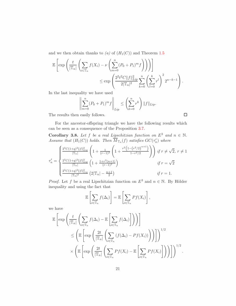
and we then obtain thanks to (a) of (H1(C)) and Theorem 1.5
E
[exp
(t
|Tn|
(∑
i∈Tn
f(Xi)− ν
(n∑
m=0
(P0 + P1)mf
)))]
≤ exp
22t2C‖f‖2Lip
2|Tn|2n∑
k=0
(k∑
l=0
rl
)2
2n−k−1
.
In the last inequality we have used∥∥∥∥∥
n∑
m=0
(P0 + P1)mf
∥∥∥∥∥Lip
≤(
n∑
k=0
rk
)‖f‖Lip.
The results then easily follows.
For the ancestor-offspring triangle we have the following results whichcan be seen as a consequence of the Proposition 3.7.
Corollary 3.8. Let f be a real Lipschitzian function on E3 and n ∈ N.Assume that (H1(C)) holds. Then MTn(f) satisfies GC(τ ′n) where
τ ′n =
23C(1+q)2‖f‖2Lip
|Tn|
(1 + 1
(r−1)2
(1 +
r2(
1−(r2/2)n+1
)
1−r2/2
))if r 6=
√2, r 6= 1
23C(1+q)2‖f‖2Lip
|Tn|
(1 + 1+r2(n+1)
(r−1)2
)if r =
√2
23C(1+q)2‖f‖2Lip
|Tn|2
(2|Tn| − n+1
2
)if r = 1.
Proof. Let f be a real Lipschitzian function on E3 and n ∈ N. By Holderinequality and using the fact that
E
[∑
i∈Tn
f(∆i)
]= E
[∑
i∈Tn
Pf(Xi)
],
we have
E
[exp
(t
|Tn|
(∑
i∈Tn
f(∆i)− E
[∑
i∈Tn
f(∆i)
]))]
≤(E
[exp
(2t
|Tn|
(∑
i∈Tn
(f(∆i)− Pf(Xi))
))])1/2
×(E
[exp
(2t
|Tn|
(∑
i∈Tn
Pf(Xi)− E
[∑
i∈Tn
Pf(Xi)
]))])1/2
.
21

We bound the first term of the right hand side of the previous inequality byusing the same calculations as in the first iteration of the proof of Corollary3.6. We then have
(E
[exp
(2t
|Tn|
(∑
i∈Tn
(f(∆i)− Pf(Xi))
))])1/2
≤ exp
(2t2C‖f‖2Lip|Tn|
2|Tn|2
).
For the second term, we use the proof of the Proposition 3.7 with Pf insteadof f . We then have
(E
[exp
(2t
|Tn|
(∑
i∈Tn
Pf(Xi)− E
[∑
i∈Tn
Pf(Xi)
]))])1/2
≤ exp
23t2R(1 + q)2‖f‖2Lip
2|Tn|2n∑
k=0
(k∑
l=0
rl
)2
2n−k−1
.
The results then follow by easy analysis and this ends the proof.
3.3 Deviation inequalities towards the invariant measure of
the randomly drawn chain
All the previous results do not assume any ”stability” of the Markov chainon the binary tree, whereas for usual asymptotic theorem the convergenceis towards mean of the function with respect to the invariant probabilitymeasure of the random lineage chain. To reinforce this asymptotic resultby non asymptotic deviation inequality, it is thus fundamental to be able toreplace for example E(MTn(f)) by some asymptotic quantity. This randomlineage chain is a Markov chain with transition kernel Q = (P0 + P1)/2.We shall now suppose the existence of a probability measure π such thatπQ = π. We will consider a slight modification of our main assumption andas we are mainly interested in concentration inequalities, let us focus in thep = 1 case:
Assumption 3.9 (H ′1(C)).
(a) ν ∈ T1(C);
(b) Pb(x, ·) ∈ T1(C), ∀x ∈ E, b = 0, 1 ;
22

(c) W d1 (P (x, ·, ·), P (x, ·, ·)) ≤ q d(x, x), ∀x, x ∈ E and some q > 0. And
for r0, r1 > 0 such that r0+r1 < 2, for b = 0, 1, W d1 (Pb(x, ·), Pb(x, ·)) ≤
rb d(x, x), ∀x, x ∈ E.
Under this assumption, using the convexity of W1 (see [37]), we easilysee that
W1(Q(x, ·), Q(x, ·)) ≤ r0 + r12
d (x, x) , ∀x, x
ensuring the strict contraction of Q, and then the exponential convergencetowards π in Wasserstein distance, namely (assuming that π has a firstmoment)
W1(Qn(x, ·), π) ≤
(r0 + r1
2
)n ∫d(x, y)π(dy).
Let us show that we may now control easily the distance between E(MTn(f))and π(f). Indeed, we may first remark that
E
∑
k∈Gn
f(Xk)
= ν(P0 + P1)
nf
so that assuming that f is 1-lipschitzian, and by the dual version of theWasserstein distance
∣∣E(MTn(f))− π(f)∣∣ =
1
|Tn|
∣∣∣∣∣∣
n∑
j=1
E
∑
k∈Gj
(f(Xk)− π(f)
∣∣∣∣∣∣
=1
|Tn|
∣∣∣∣∣∣
n∑
j=1
2jν
(P0 + P1
2
)j
(f − π(f))
∣∣∣∣∣∣
≤ 1
|Tn|
n∑
j=1
2jW1(νQj, π)
≤ 1
|Tn|
n∑
j=1
(r0 + r1)j
≤ cn :=
c(r0+r1
2
)n+1if r0 + r1 6= 1
c n2n+1 if r0 + r1 = 1
for some universal c, which goes to 0 exponentially fast as soon as r0+r1 < 2which was assumed in (H ′
1(C)). We may then see that for r > cn
P(MTn(f)− π(f) > r
)≤ P
(MTn(f)− E(MTn(f)) > r − cn
)
and one then applies the result of the previous subsection.
23
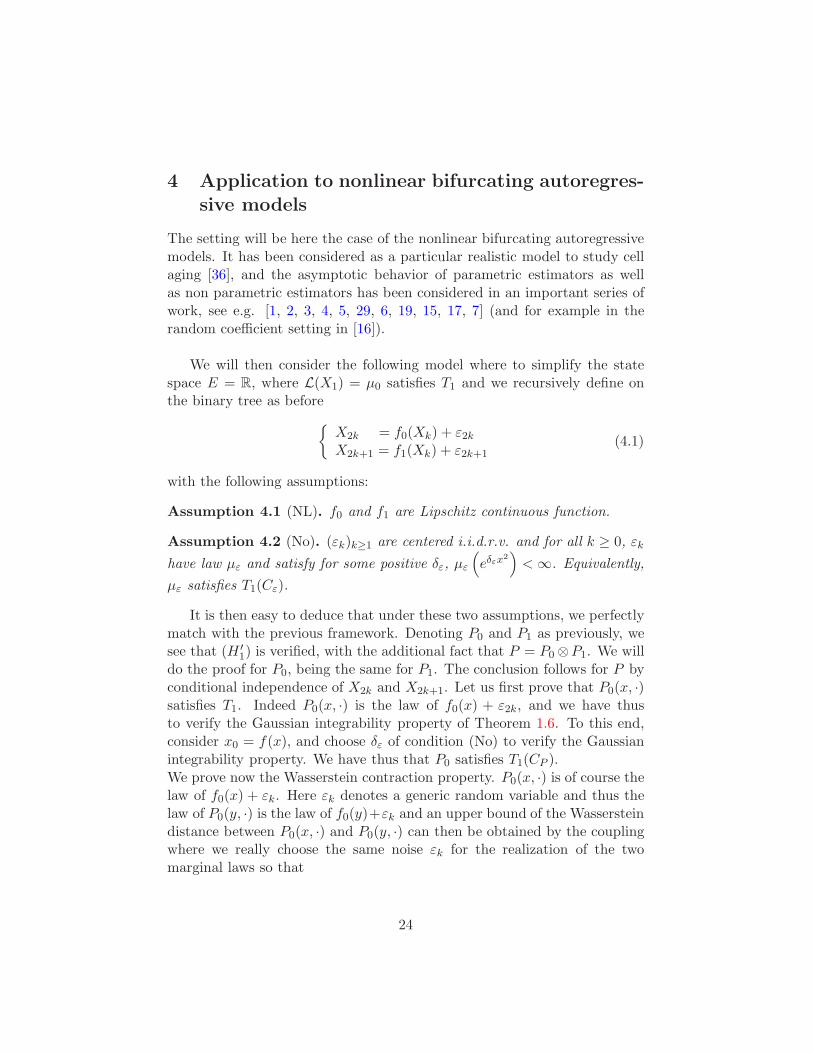
4 Application to nonlinear bifurcating autoregres-
sive models
The setting will be here the case of the nonlinear bifurcating autoregressivemodels. It has been considered as a particular realistic model to study cellaging [36], and the asymptotic behavior of parametric estimators as wellas non parametric estimators has been considered in an important series ofwork, see e.g. [1, 2, 3, 4, 5, 29, 6, 19, 15, 17, 7] (and for example in therandom coefficient setting in [16]).
We will then consider the following model where to simplify the statespace E = R, where L(X1) = µ0 satisfies T1 and we recursively define onthe binary tree as before
X2k = f0(Xk) + ε2kX2k+1 = f1(Xk) + ε2k+1
(4.1)
with the following assumptions:
Assumption 4.1 (NL). f0 and f1 are Lipschitz continuous function.
Assumption 4.2 (No). (εk)k≥1 are centered i.i.d.r.v. and for all k ≥ 0, εk
have law µε and satisfy for some positive δε, µε
(eδεx
2)< ∞. Equivalently,
µε satisfies T1(Cε).
It is then easy to deduce that under these two assumptions, we perfectlymatch with the previous framework. Denoting P0 and P1 as previously, wesee that (H ′
1) is verified, with the additional fact that P = P0 ⊗P1. We willdo the proof for P0, being the same for P1. The conclusion follows for P byconditional independence of X2k and X2k+1. Let us first prove that P0(x, ·)satisfies T1. Indeed P0(x, ·) is the law of f0(x) + ε2k, and we have thusto verify the Gaussian integrability property of Theorem 1.6. To this end,consider x0 = f(x), and choose δε of condition (No) to verify the Gaussianintegrability property. We have thus that P0 satisfies T1(CP ).We prove now the Wasserstein contraction property. P0(x, ·) is of course thelaw of f0(x) + εk. Here εk denotes a generic random variable and thus thelaw of P0(y, ·) is the law of f0(y)+εk and an upper bound of the Wassersteindistance between P0(x, ·) and P0(y, ·) can then be obtained by the couplingwhere we really choose the same noise εk for the realization of the twomarginal laws so that
24

Let f be any Lipschitz function such that ‖f‖Lip ≤ 1
∣∣∣∣∫
Sf(z)P0(x, dz) −
∫
Sf(z)P0(y, dz)
∣∣∣∣ = E [f (f0(x) + ε1)− f (f0(y) + ε1)]
≤ ‖f‖Lip|f0(x)− f0(y)|.
By the Monge-Kantorovitch duality expression of the Wasserstein distance,one has then
W1(P0(x, ·), P0(y, ·)) ≤ |f0(x)− f0(y)| ≤ ‖f0‖Lip|x− y|.
Thus under (NL) and (No), our model fits in the framework of the pre-vious section with q = ‖f0‖Lip + ‖f1‖Lip, r0 = ‖f0‖Lip and r1 = ‖f1‖Lip.We will be interested here in the non parametric estimation of the autore-gression functions f0 and f1, and we will use Nadaraya-Watson kernel typeestimator, as considered in [9]. Let K be a kernel satisfying the followingassumption.
Assumption 4.3 (Ker). The function K is non negative, has compact sup-port [−R,R], is Lipschitz continuous with constant ‖K‖Lip and such that∫K(z)dz = 1.
Let us also introduce as usual a bandwidth hn which will be taken tosimplify as hn := |Tn|−α for some 0 < α < 1. The Nadaraya-Watsonestimators are then defined as for x ∈ R
f0,n(x) :=
1
|Tn|hn∑
k∈Tn
K
(Xk − x
hn
)X2k
1
|Tn|hn∑
k∈Tn
K
(Xk − x
hn
)
f1,n(x) :=
1
|Tn|hn∑
k∈Tn
K
(Xk − x
hn
)X2k+1
1
|Tn|hn∑
k∈Tn
K
(Xk − x
hn
) .
Let us focus on f0, as it will be exactly the same for f1 and fix x ∈ R. We willbe interested here in deviation inequalities of f0,n(x) with respect to f(x).One has to face two problems. First it is an autonormalized estimator. It willbe dealt with considering deviation inequalities for the numerator and de-nominator separately and reunite them. Secondly (x, y) → K(x)y is in fact
25
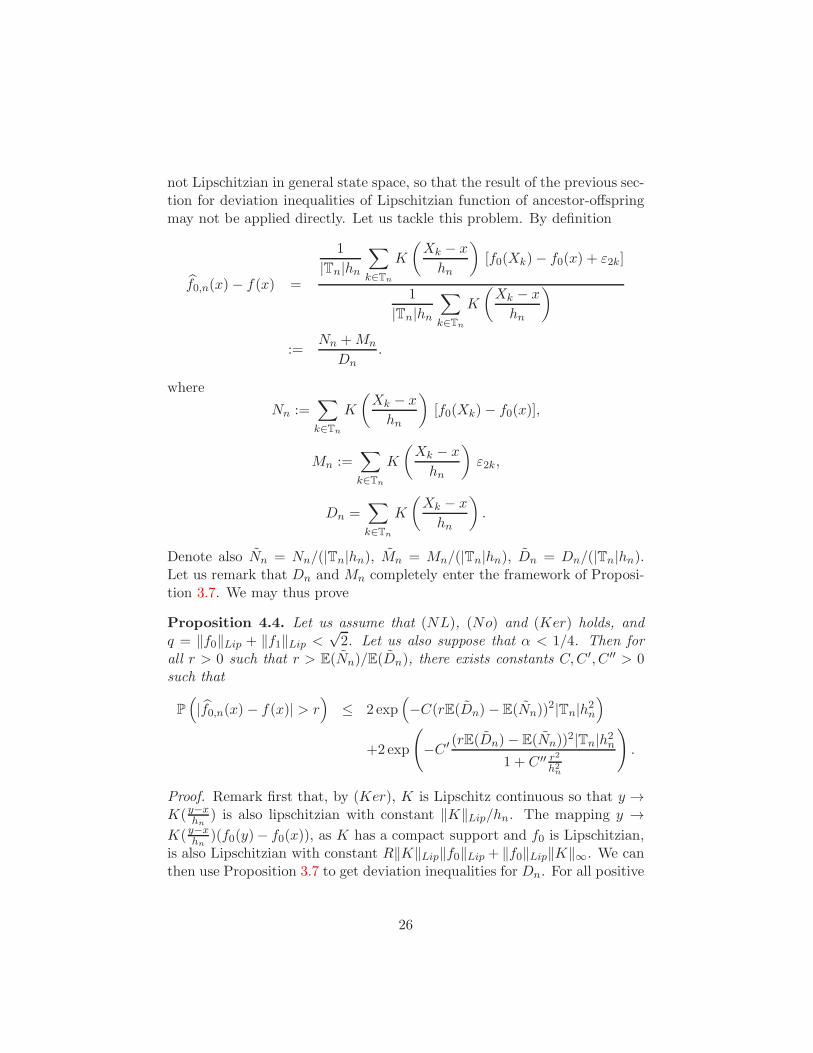
not Lipschitzian in general state space, so that the result of the previous sec-tion for deviation inequalities of Lipschitzian function of ancestor-offspringmay not be applied directly. Let us tackle this problem. By definition
f0,n(x)− f(x) =
1
|Tn|hn∑
k∈Tn
K
(Xk − x
hn
)[f0(Xk)− f0(x) + ε2k]
1
|Tn|hn∑
k∈Tn
K
(Xk − x
hn
)
:=Nn +Mn
Dn.
where
Nn :=∑
k∈Tn
K
(Xk − x
hn
)[f0(Xk)− f0(x)],
Mn :=∑
k∈Tn
K
(Xk − x
hn
)ε2k,
Dn =∑
k∈Tn
K
(Xk − x
hn
).
Denote also Nn = Nn/(|Tn|hn), Mn = Mn/(|Tn|hn), Dn = Dn/(|Tn|hn).Let us remark that Dn and Mn completely enter the framework of Proposi-tion 3.7. We may thus prove
Proposition 4.4. Let us assume that (NL), (No) and (Ker) holds, andq = ‖f0‖Lip + ‖f1‖Lip <
√2. Let us also suppose that α < 1/4. Then for
all r > 0 such that r > E(Nn)/E(Dn), there exists constants C,C ′, C ′′ > 0such that
P
(|f0,n(x)− f(x)| > r
)≤ 2 exp
(−C(rE(Dn)− E(Nn))
2|Tn|h2n)
+2exp
(−C ′ (rE(Dn)− E(Nn))
2|Tn|h2n1 + C ′′ r2
h2n
).
Proof. Remark first that, by (Ker), K is Lipschitz continuous so that y →K(y−x
hn) is also lipschitzian with constant ‖K‖Lip/hn. The mapping y →
K(y−xhn
)(f0(y)− f0(x)), as K has a compact support and f0 is Lipschitzian,is also Lipschitzian with constant R‖K‖Lip‖f0‖Lip + ‖f0‖Lip‖K‖∞. We canthen use Proposition 3.7 to get deviation inequalities for Dn. For all positive
26
r there exists a constant L (explicitly given through Proposition 3.7), suchthat
P(|Dn − E(Dn)| > r|Tn|hn) ≤ 2 exp(−Lr2|Tn|h4n/‖K‖2Lip
).
For Nn+Mn we cannot directly apply Proposition 3.7 due to the successivedependence of Xk at generation n and ε2k of generation n − 1. But as weare interested in deviation inequalities, we may split the deviation comingfrom each term. For Nn, it is once again a simple application of Proposition3.7,
P(|Nn−E(Nn)| > r|Tn|hn) ≤ 2 exp
( −Lr2|Tn|h2n(R‖K‖Lip‖f0‖Lip + ‖f0‖Lip‖K‖∞)2
).
Note that ε2k is independent of Xk, and centered so that E(Mn) = 0,and satisfies a transportation inequality. Note also that K is bounded. Bysimple conditioning argument, we may control the Laplace transform of Mn
quite simply. We then have for all positive r
P(|Mn| > r|Tn|hn) ≤ 2 exp
(−r2
|Tn|h2n‖K‖2∞2Cε
).
However, we cannot use directly these estimations as the estimator isautonormalized. Instead
P
(f0,n(x)− f(x) > r
)
≤ P(Nn + Mn > rDn)
≤ P
(Nn − E(Nn)− r(Dn − E(Dn)) + Mn > rE(Dn)− E(Nn)
)
≤ P
(Nn − E(Nn)− r(Dn − E(Dn) > (rE(Dn)− E(Nn))/2
)
+P
(Mn > (rE(Dn)− E(Nn))/2
)
Remark now to conclude that K((y−x)/hn)(f(y)−f(x))+K((y−x)/hn) is(R‖K‖Lip‖f0‖Lip + ‖f0‖Lip‖K‖∞ + r‖K‖Lip/hn)-Lipschitzian, and we maythen proceed as before.
Remark 4.5. In order to get fully practical deviation inequalities, let usremark that
E
[Dn
]=
1
|Tn|hn
n∑
m=0
2mµ0QmH −→
n→+∞ν(x)
27

where H(y) = K((y − x)/hn), ν(·) is the invariant density of the Markovchain associated to a random lineage and
E
[Nn
]=
1
|Tn|hn
n∑
m=0
2m (µ0Qm(Hf0)− f0(x)µ0Q
mH) −→n→+∞
0.
We refer to [9] for quantitative versions of these limits.
Remark 4.6. Of course this non parametric estimation is in some senseincomplete, as we would have liked to consider a deviation inequality forsupx |f0,n(x) − f0(x)|. The problem is somewhat much more complicatedhere, as the estimator is self normalized. However, it is a crucial problemthat we will consider in the near future. For some ideas which could beuseful here, let us cite the results of [12] for (uniform) deviation inequal-ities for estimators of density in the i.i.d. case, and to [22] for control ofthe Wasserstein distance of the empirical measure of i.i.d.r.v. or of Markovchains.
Remark 4.7 (Estimation of the T-transition probability). We assume thatthe process has as initial law, the invariant probability ν. We denote by f thedensity of (X1,X2,X3). For the estimation of f , we propose the estimatorfn defined by
fn(x, y, z) =1
|Tn|hn∑
k∈Tn
K
(x−Xk
hn
)K
(y −X2k
hn
)K
(z −X2k+1
hn
).
An estimator of the T-probability transition is then given by
Pn (x, y, z) =fn(x, y, z)
Dn
.
For x, y, z ∈ R, one can observe that the function G defined on R3 by
G(u, v, w) = K
(x− u
hn
)K
(y − v
hn
)K
(z − w
hn
)
is Lipschitzian with ‖G‖Lip ≤ (‖K‖2∞‖K‖Lip)/hn. We have
Pn (x, y, z) − P (x, y, z) =fn(x, y, z) − f(x, y, z)
Dn
+f(x, y, z)(ν(x) − Dn)
ν(x)Dn
.
Now using the decomposition
fn(x, y, z) − f(x, y, z) =(fn(x, y, z) − E
[fn(x, y, z)
])
+(E
[fn(x, y, z)
]− f(x, y, z)
)
28

and the convergence of E[fn(x, y, z)
]to f(x, y, z), we obtain a deviation
inequality for |Pn (x, y, z)−P (x, y, z)| similar to that obtained at the Propo-sition 4.4.
When the density gε of (ε2, ε3) is known, another strategy for the esti-mation of the T-transition probability is to observe that P (x, y, z) = gε(y−f0(x), z − f1(x)). An estimator of P (x, y, z) is then given by Pn(x, y, z) =gε(y− f0,n(x), z− f1,n(x)) where f0,n and f1,n are estimators defined above.If gε is Lipschitzian, we have
|Pn (x, y, z)− P (x, y, z)| ≤ ‖gε‖Lip(|f0,n(x)− f0(x)|+ |f1,n(x)− f1(x)|
)
and the deviation inequalities for |Pn (x, y, z) − P (x, y, z)| are thus of thesame order that those given by the Proposition 4.4.
Acknowledgements
S.V. Bitseki Penda sincerely thanks Labex Mathematiques Hadamard. A.Guillin was supported by the French ANR STAB project.
References
[1] I. V. Basawa and R. M. Huggins. Extensions of the bifurcating autore-gressive model for cell lineage studies. J. Appl. Probab, 36, 4:1225–1233,1999.
[2] I. V. Basawa and R. M. Huggins. Inference for the extended bifurcatingautoregressive model for cell lineage studies. Aust. N. Z. J. Stat, 42,4:423–432, 2000.
[3] I. V Basawa and J. Zhou. Non-Gaussian bifurcating models and quasi-likelihood estimation. J. Appl. Probab, 41A:55–64, 2004.
[4] I. V. Basawa and J. Zhou. Least-squares estimation for bifurcatingautoregressive processes. Statist. Probab.Lett., 1:77–88, 2005.
[5] I. V. Basawa and J. Zhou. Maximum likelihood estimation for a first-order bifurcating autoregressive process with exponential errors. J.Time Ser. Anal., 26, 6:825–842, 2005.
[6] B. Bercu, B. De Saporta, and A. Gegout-Petit. Asymptotic analysis forbifurcating autoregressive processes via a martingale approach. Elec-tronic. J. Probab., 14:2492–2526, 2009.
29

[7] S. V. Bitseki Penda and H. Djellout. Deviation inequalities and moder-ate deviations for estimators of parameters in bifurcating autoregressivemodels. Annales de l’IHP-PS, 50(3):806–844, 2014.
[8] S. V. Bitseki Penda, H. Djellout, and A. Guillin. Deviation inequalities,moderate deviations and some limit theorems for bifurcating Markovchains with application. The Annals of Applied Probability, 24(1):235–291, 2014.
[9] S. V. Bitseki Penda and A. Olivier. Asymptotic behavior of nonpara-metric estimators in nonlinear bifurcating autoregressive models. Inpreparation, 2015.
[10] S.V. Bitseki Penda. Deviations inequalities for bifurcating markovchains on galton- watson tree. In revision for ESAIM P/S, 2014.
[11] S. Bobkov and F. Gotze. Exponential integrability and transportationcost related to logarithmic sobolev inequalities. J. Funct. Anal., 163:1–28, 1999.
[12] F. Bolley, A. Guillin, and C. Villani. Quantitative concentration in-equalities for empirical measures on non-compact spaces. Probab. The-ory Related Fields, 137(3-4):541–593, 2007.
[13] P. Cattiaux and A. Guillin. On quadratic transportation cost inequal-ities. J. Math. Pures Appl. (9), 86(4):341–361, 2006.
[14] P. Cattiaux, A. Guillin, and L. Wu. A note on Talagrand’s transporta-tion inequality and logarithmic Sobolev inequality. Probab. Theory Re-lated Fields, 148(1-2):285–304, 2010.
[15] B. De Saporta, A Gegout-Petit, and L. Marsalle. Asymmetry tests forbifurcating auto-regressive processes with missing data. preprint, page2011.
[16] B. De Saporta, A Gegout-Petit, and L. Marsalle. Random coefficientsbifurcating autoregressive processes. arXiv:1205.3658v1 [math.PR],page 2012.
[17] B. De Saporta, A. Gegout-Petit, and L. Marsalle. Parameters estima-tion for asymmetric bifurcating autoregressive processes with missingdata. Electronic Journal of Statistics, 5:1313–1353, 2011.
30

[18] B. De Saporta, A. Gegout-Petit, and L. Marsalle. Random coefficientsbifurcating autoregressive processes. ESAIM PS, 18:365–399, 2014.
[19] J. F. Delmas and L. Marsalle. Detection of cellular aging in Galton-Watson process. Stochastic Processes and their Applications, 120:2495–2519, 2010.
[20] H. Djellout, A. Guillin, and L. Wu. Transportation cost-informationinequalities and applications to random dynamical systems and diffu-sions. Annals of Probability, 32, No. 3B:2702–2732, 2004.
[21] M. Doumic, M. Hoffmann, N. Krell, and L. Robert. Statistical estima-tion of a growth-fragmentation model observed on a genealogical tree.Bernoulli, to appear, 2014.
[22] N. Fournier and A. Guillin. On the rate of convergence in Wassersteindistance of the empirical measure. Probab. Theory Related Fields, Toappear, 2015.
[23] N. Gozlan. Integral criteria for transportation-cost inequalities. Elec-tron. Comm. Probab., 11:64–77 (electronic), 2006.
[24] N. Gozlan. A characterization of dimension free concentration in termsof transportation inequalities. Ann. Probab., 37(6):2480–2498, 2009.
[25] N. Gozlan and C. Leonard. A large deviation approach to sometransportation cost inequalities. Probab. Theory Related Fields, 139(1-2):235–283, 2007.
[26] N. Gozlan and C. Leonard. Transport inequalities. A survey. MarkovProcess. Related Fields, 16(4):635–736, 2010.
[27] N. Gozlan, C. Roberto, and P-M. Samson. A new characterizationof Talagrand’s transport-entropy inequalities and applications. Ann.Probab., 39(3):857–880, 2011.
[28] A. Guillin, C. Leonard, L. Wu, and N. Yao. Transportation-informationinequalities for Markov processes. Probab. Theory Related Fields, 144(3-4):669–695, 2009.
[29] J. Guyon. Limit theorems for bifurcating Markov chains. applicationto the detection of cellular aging. Ann. Appl. Probab., Vol. 17, No.5-6:1538–1569, 2007.
31

[30] J. Guyon, A. Bize, G. Paul, E.J. Stewart, J.F. Delmas, and F. Taddei.Statistical study of cellular aging. CEMRACS 2004 Proceedings,ESAIM Proceedings, 14:100–114, 2005.
[31] M. Ledoux. The concentration of measure phenomenon. MathematicalSurveys and Monographs, 89. American Mathematical Society, Provi-dence, RI, 2001.
[32] K. Marton. A simple proof of the blowing-up lemma. IEEE Transac-tions on Information Theory, 32:445–446, 1986.
[33] K. Marton. Bounding d-distance by informational divergence: a way toprove measure concentration. Annals of Probability, 24:857–866, 1996.
[34] K. Marton. A measure concentration inequality for contracting Markovchains. Geom. Funct. Anal., 6:556–571, 1997.
[35] P. Massart. Concentration inequalities and model selection. LectureNotes in Mathematics, 1896. Springer, Berlin, 2007.
[36] E. J. Stewart, R. Madden, G. Paul, and F.. Taddei. Aging and deathin an organism that reproduces by morphologically symmetric division.PLoS Biol, 3(2):e45, 2005.
[37] C. Villani. Optimal transport, volume 338 of Grundlehren der Math-ematischen Wissenschaften [Fundamental Principles of MathematicalSciences]. Springer-Verlag, Berlin, 2009. Old and new.
32