HAL Id: tel-00944511https://tel.archives-ouvertes.fr/tel-00944511

Submitted on 10 Feb 2014

HAL is a multi-disciplinary open accessarchive for the deposit and dissemination of sci-entific research documents, whether they are pub-lished or not. The documents may come fromteaching and research institutions in France orabroad, or from public or private research centers.

L’archive ouverte pluridisciplinaire HAL, estdestinée au dépôt et à la diffusion de documentsscientifiques de niveau recherche, publiés ou non,émanant des établissements d’enseignement et derecherche français ou étrangers, des laboratoirespublics ou privés.

Transport and Density Fluctuations in DisorderedSystems: Appliations to Atmospheric Dispersion

Rehab Bitane

To cite this version:Rehab Bitane. Transport and Density Fluctuations in Disordered Systems: Appliations to Atmo-spheric Dispersion. Fluid mechanics [physics.class-ph]. Université Nice Sophia Antipolis, 2012. En-glish. tel-00944511

Université deNi eSophiaAntipolis - UFR S ien esE ole Do torale de S ien es Fondamentales et AppliquéesTHES I Sto obtain the title ofPh.D. in S ien esof the University of Ni e-Sophia AntipolisDis ipline : Physi spresented and defended byRehab BitaneTransport and Density Flu tuationsin Disordered SystemsAppli ations to Atmospheri Dispersiondefended on the 22nd of November 2012Committee :Mr. Mi kaël Bourgoin RefereeMs. Alessandra Lanotte RefereeMr. Mar -Étienne Bra het Member of the CommiteeMr. Alain Pumir President of the CommiteeMr. Alain Noullez AdvisorMr. Jérémie Be Co-advisor

Université deNi eSophiaAntipolis - UFR S ien esE ole Do torale de S ien es Fondamentales et AppliquéesTHÈSEpour obtenir le titre deDo teur en S ien esde l'Université de Ni e-Sophia AntipolisDis ipline : Physiqueprésentée et soutenue parRehab BitaneTransport et Flu tuations de Densitédans les Systèmes DésordonnésAppli ations à la Dispersion AtmophériqueThèse dirigée par Alain NOULLEZet o-dirigée par Jérémie BECsoutenue le 22 Novembre 2012Jury :M. Mi kaël Bourgoin RapporteurMme. Alessandra Lanotte RapporteurM. Mar -Étienne Bra het ExaminateurM. Alain Pumir PrésidentM. Alain Noullez Dire teurM. Jérémie Be Co-dire teur

i

A mia nonna Imma olata

ii

iiiRésuméLe transport turbulent de parti ules est un phénomène important qui inter-vient dans de nombreux pro essus naturels et industriels. Comprendre sespropriétés et, en parti ulier, la réation de grandes u tuations de densité,est fondamental pour améliorer les modèles et aner les prévisions. Celareprésente de nombreux enjeux é onomiques, environnementaux et de santé.Une étude Lagrangienne de la séparation de paires de tra eurs a été menée ens'appuyant sur l'analyse des données de simulations numériques à très hauterésolution. Elle a permis de souligner les défaillan es des appro hes de type hamp moyen qui sont à la base des modèles les plus ouramment utilisés.Pour la séparation, on onstate que la transition entre le régime balistique deBat helor et le régime explosif de Ri hardson a lieu à des temps données parle temps moyen de dissipation de l'énergie inétique turbulente. Aussi, il estmontré que la loi de Ri hardson peut s'interpréter omme un omportementdiusif des diéren es de vitesse. Des arguments phénoménologiques perme-ttent d'interpréter et eet par la dé orrélation de diéren es d'a élérationet la stationnarité aux temps longs du taux lo al de transfert d'énergie iné-tique. Les moments d'ordres élevés de la séparation et de la vitesse sontaussi étudiés pour aborder la question des événements violents dans la dis-tribution des distan es. Enn, un modèle d'éje tion de masse est proposéet utilisé pour examiner les u tuations de la densité de parti ules lourdestransportées dans un environnement aléatoire.SummaryThe turbulent transport of parti les is an important phenomena whi h ap-pears in many natural and industrial pro esses. Understanding its properties,and, in parti ular, the reation of strong density u tuations, is fundamentalto improve models and rene fore asts. This an lead to signi ant benetsin issues related to e onomi s, the environmental and health. A Lagrangianstudy of the tra er pair separation was arried out with the help of highresolution data analysis. This allowed us to point out the weaknesses of themean-eld approa hes on whi h most models are based. For the separation,it is found that the transition from the regime of Bat helor (or ballisti ) tothat of Ri hardson (or explosive) o urs at times given by those typi al ofthe turbulent kineti energy dissipation. It is also found that Ri hardson'slaw an be reinterpreted in terms of diusive behaviour of the velo ity dier-en es. Phenomenologi al arguments allow us to explain this ee t throughthe de orrelation of the a eleration dieren es and the stationarity of the

ivkineti energy transfer ratio at large times. The high-order moments of bothseparation and velo ity are also investigated to address the question of vio-lent events" in the distribution of the distan es. Finally, a one-dimensionalmass eje tion model is proposed and used to examine the density u tuationsof heavy parti les transported by the random environment.

Contents1 Introdu tion 12 Basi on epts in turbulen e 92.1 Phenomenology of turbulent ows . . . . . . . . . . . . . . . . 92.1.1 Kolmogorov 1941 theory . . . . . . . . . . . . . . . . . 102.1.2 Similarity and s ale invarian e . . . . . . . . . . . . . . 122.2 Energy budgets and transfers in turbulen e . . . . . . . . . . . 132.2.1 Dire t and inverse as ades . . . . . . . . . . . . . . . 152.2.2 Energy and enstrophy spe tra . . . . . . . . . . . . . . 182.2.3 Intermitten y . . . . . . . . . . . . . . . . . . . . . . . 202.3 Mixing in a turbulent ow . . . . . . . . . . . . . . . . . . . . 213 Parti le Transport 253.1 Dynami s of tiny parti les in turbulent ows . . . . . . . . . . 263.1.1 Equations of motion . . . . . . . . . . . . . . . . . . . 263.1.2 Generalities on sto hasti pro esses . . . . . . . . . . . 283.1.3 Single-parti le diusion in turbulent ow . . . . . . . . 323.2 Con entration properties . . . . . . . . . . . . . . . . . . . . . 343.2.1 Flu tuations of an adve ted passive s alar . . . . . . . 343.2.2 Preferential on entration of inertial parti les . . . . . 394 Diusivity in turbulent pair dispersion 434.1 The regimes of tra er separation . . . . . . . . . . . . . . . . . 444.1.1 Ri hardson's diusive approa h . . . . . . . . . . . . . 454.1.2 Bat helor's ballisti regime . . . . . . . . . . . . . . . . 474.2 Times ales of two-parti le dispersion . . . . . . . . . . . . . . 484.2.1 Settings of the numeri al simulations . . . . . . . . . . 484.2.2 Times ale of departure from Bat helor's regime . . . . 524.2.3 Convergen e to the super-diusive behavior . . . . . . 554.3 Statisti s of velo ity dieren es . . . . . . . . . . . . . . . . . 584.3.1 A diusive behavior? . . . . . . . . . . . . . . . . . . . 58v

vi CONTENTS4.3.2 Geometry of longitudinal velo ities . . . . . . . . . . . 614.4 Lo al dissipation and velo ity diusion . . . . . . . . . . . . 644.4.1 Stationarity of res aled velo ity dieren es . . . . . . . 654.4.2 Statisti s of a eleration dieren es . . . . . . . . . . . 684.4.3 A one-dimensional sto hasti model . . . . . . . . . . . 725 Geometry and violent events in turbulent relative motion 815.1 High-order statisti s . . . . . . . . . . . . . . . . . . . . . . . 825.1.1 S aling regime in the statisti s of distan es . . . . . . . 825.1.2 Intermittent distributions of velo ity dieren es . . . . 865.2 Memory in large-distan e statisti s . . . . . . . . . . . . . . . 895.3 Fra tal distribution at small distan es . . . . . . . . . . . . . 935.4 Summary and perspe tives on the problem of pair dispersion . 976 Mass u tuations and diusions in random environments 1016.1 Flu tuations in heavy parti le density . . . . . . . . . . . . . . 1026.2 Generality on random walks . . . . . . . . . . . . . . . . . . . 1046.3 Des ription of the model . . . . . . . . . . . . . . . . . . . . . 1066.4 Statisti al properties of the random environment . . . . . . . 1096.4.1 Denition of the random eje tion rate . . . . . . . . . . 1096.4.2 Numeri al methods . . . . . . . . . . . . . . . . . . . . 1106.4.3 Phenomenology and dimensionless parameters . . . . . 1126.5 Diusive properties . . . . . . . . . . . . . . . . . . . . . . . 1156.5.1 Diusion oe ient . . . . . . . . . . . . . . . . . . . . 1166.5.2 PDF of displa ement . . . . . . . . . . . . . . . . . . . 1176.6 Density u tuations . . . . . . . . . . . . . . . . . . . . . . . . 1216.6.1 Smooth random environments . . . . . . . . . . . . . . 1226.6.2 Non-smooth random environment . . . . . . . . . . . . 1286.7 S ale invarian e of the mass density eld . . . . . . . . . . . . 1316.8 Brief summary and on lusions . . . . . . . . . . . . . . . . . 1337 Con lusions and perspe tives 137

Chapter 1Introdu tionAlmost all natural and industrial uid ows are usually in a turbulent state.Their study has always attra ted mu h attention in order to understand, forexample, the hydro or aerodynami al properties of obje ts, to model windsin meteorology or uxes in fa tory devi es, and to quantify the times alesat whi h transported spe ies are mixed and dispersed. During the lasttwo de ades turbulent transport has gathered a growing interest in the s i-enti ommunity. This is due to the development of new so ietal on- erns related to pollution and limate hange and, at the same time, tothe emergen e of the s ienti paradigm of Lagrangian turbulen e. Tur-bulent transport is indeed ubiquitous in atmospheri physi s, o eanographyand astrophysi s [Csanady, 1973, Seinfeld & Pandis, 2006, Battaner, 1996.It plays a ru ial role in modeling the dispersion of vol ani ashes [Peterson& Dean, 2008 or of pollutants [Arya, 1999,Cooper & Alley, 2002, the dy-nami s of plankton populations in seas [Lewis & Bala, 2006, the formationof louds [Pinsky & Khain, 1997, the initiation of rain [Shaw, 2003 or theearly stages of planet formation [De Pater & Lissauer, 2001,Charnoz et al.,2011. Illustrations of su h appli ations are shown in Fig. 1.1. The phenom-ena o urring in the atmosphere are the obje t of intense studies be ause, inaddition to important e onomi al and e ologi al impli ations, their pre iseunderstanding is needed to design e ient and reliable models in meteorol-ogy and limate s ien es. In parallel to su h a growth of interest, the lastde ades witnessed the development of new theoreti al approa hes for theproblem of turbulent transport, or of Lagrangian turbulen e. Su h funda-mental ontributions have used tools taken from statisti al physi s and eldtheory [Shraiman et al., 2000,Falkovi h et al., 2001,Cardy et al., 2008 andled to important results related, for instan e, to the anomalous s aling of pas-sive tra ers [Bernard et al., 1996, to the improvement of ollision kernels forwarm louds [Falkovi h et al., 2002, and to the statisti al properties of vor-1

2 1. Introdu tionti ity ontours in two-dimensional turbulen e [Bernard et al., 2006. Theseadvan es were intri ately onne ted to simultaneous experimental develop-ments. Re ent opti al and ele troni te hnologies have been used to improveLagrangian measurement te hniques and to tra k transported parti les inhighly turbulent ows. Breakthroughs were then made on the determinationof uid element a elerations [La Porta et al., 2001, on the study of rela-tive dispersion [Ott & Mann, 2000,Bourgoin et al., 2006 and on the s alingproperties of Lagrangian velo ity in rements [Arnéodo et al., 2008.The work presented in this thesis manus ript has the long-term obje tiveto ontribute to the study of atmospheri dispersion, with a parti ular em-phasis on the transport of parti ulate pollutants. Su h pollutants originateeither from natural sour es (suspension of dust by wind erosion, of salt byseawater evaporation, dispersion of pollen, of vol an ash, . . . ) or from hu-man a tivities ( ombustion of organi ompounds, dispersion of inse ti idesused in agri ulture, emission of industrial and nu lear wastes, . . . ) [Harrison& Perry, 1986. These parti ulate atmospheri pollutants are often alledaerosols, as they are solid parti les suspended in the air. They have dire tand indire t ee ts on limate, whi h are still ontroversial and the sour eof many un ertainties [Pilewskie, 2007,Stevens & Feingold, 2009. Also, theparti ulate pollutants represent a hazard for health. Their harmfulness oftendepends on their size [Valavanidis et al., 2008. As we will see in more detailslater, very small parti les (with sizes of the order of 1µm or smaller) areextremely dangerous be ause they an rea h and settle into the pulmonaryalveoli, ausing serious respiratory diseases. These parti les are so small that,in good approximation, size ee ts do not enter their dynami s. They fol-low the uid ow as tra e markers and are usually referred to as Lagrangiantra ers. In addition, when they are su iently dilute, these small parti lesdo not inuen e the uid motion and one then talks of passive tra ers.Turbulent transport enhan es the dispersion of spe ies. In addition tomole ular diusion and adve tion by a mean ow, the uid ow u tuationsprovide another me hanism of mixing, usually alled turbulent dispersion,whi h is orders of magnitude more e ient. If we onsider, for instan e,the smoke of a igarette in a room, experien e suggests that few se onds areenough to diuse its smell everywhere. However, even with the most a - urate estimations on smoke diusivity and on the onve tion ee ts due totemperature dieren es between smoke and air, one would obtain a diusiontime of the order of hours. Su h a dis repan y o urs when one negle tsthe ee ts of turbulen e. Sin e the pioneering work of Reynolds in 1883,there have been many eorts to understand and model how turbulent mix-ing interfere with both the large-s ale adve tion by a mean ow and thesmall-s ale mole ular diusivity. In a developed turbulent ow, the s ales

3

(a) Ash and dust plume ar-ried away from Etna vol anoin Si ily. (b) Radioa tive leak after there ent disaster in FukushimaDaii hi nu lear omplex. ( ) Artist view of a pro-toplanetary disk gravitat-ing around a young star.Credit: NASA/JPL-Calte h

(d) Phytoplankton bloom inthe bay of Bis ay. Credit: NASA (e) Clouds formation in thehigh atmosphere. (f) Pollution due to indus-trial a tivities.Figure 1.1: Examples of situations involving turbulent parti le transport.asso iated to these two pro esses are generally widely separated and the tur-bulen e spans all the intermediate range between them. This led E kart in1948 to de ompose the pro ess of turbulent dispersion in three main steps.The rst on erns large s ales, where parti les are entrained, the se ond isresponsible for the mixing pro ess that happens at intermediate s ales, andthe last step is at small s ales where stret hing by the uid strain reateslarge on entration gradients and diusion be omes important.The study of Lagrangian transport aims at des ribing the pro esses o - urring in the intermediate range of length s ales where turbulen e is at play.Mu h work has been devoted to the study of tra er dynami s in turbulentows. However, be ause of the large span of s ales overed by turbulen e(from millimeters to hundreds of meters in the atmosphere), the predi tion

4 1. Introdu tion

(a) (b)Figure 1.2: (a) S hemati illustration of trapping events in turbulent ow.A parti le nds along its path several vorti es (here indi ated by squares)that a t like traps and interrupt the traje tory. (b) Gaussian vs meanderingplume. The snapshot shows the positions of tra er parti les (bla k dots)downstream a sour e. The plume ontains regions with lo al high densitythan annot be predi ted from the solution of the mean eld approximation( olor ba kground).tools, whi h are expe ted to be operative in on rete situations, have to relyon modeling. Many approa hes have thus been investigated in order to designe ient and reliable models for turbulent tra er dispersion and onsequentlythe time evolution of their on entration elds (see, for instan e, [Monin &Yaglom, 1971,Csanady, 1973,Majda & Kramer, 1999,Pope, 2000). Despitethe evident progresses that have been a hieved, most of the models urrentlyused to predi t for instan e air quality, provide pollutant on entration fore- asts that are rather rough sin e they are simply based on the estimations ofthe average on entration elds. Transport is indeed usually treated via theso- alled mean-eld approa hes [Opper & Saad, 2001. They onsist in ap-proximating the transport through a ombination of adve tion by the meanwind velo ity and diusion to model the ee ts of airow turbulent u tua-tions. These te hniques give a eptable results on long-term averages. Theresulting estimations are su ient in many appli ations, as for instan e wheninterested in the mean exposure to a given pollutant. In addition, they donot require sophisti ated modeling as the balan e between a ura y and ef- ien y is generally satisfa tory. This partly explains the gap that urrently

5exists between state-of-the-art models and pra ti al implementations.However, in some ases, one ould be interested in estimating the u -tuations that originate from the omplex stru ture of the turbulent ow.An instan e is the risk that a lo al pollutant on entration ex eeds a giventhreshold. Often, lo al unexpe ted on entration u tuations an indeedprodu e serious damages on health and predi ting them would give greatbenets for safety monitoring. The re ent eruption of the I elandi vol anoEyjafjallajökull in 2010 is another instan e where su h short omings hadan important e onomi al impa t. The inability of meteorologi al models topredi t the likelihood that an air raft meets a on entrated ash pu led to ompletely lose the North-European air tra . Thus the importan e of thestrong u tuations of mass on entration elds in monitoring and predi t-ing atmospheri dispersion annot be underestimated. In su h situations,the relevant s ales are then mu h smaller than those typi ally resolved bymodels. In addition, the information on an average value is not su ient todire tly determine the amplitude and the nature of the u tuations. High on entrations are asso iated to the values of the tails of the probability dis-tribution rather than to its ore. A typi al situation that an be en ounteredin turbulent transport is shown in Fig. 1.2(b), whi h represents the average on entration ( olored ba kground), together with the instantaneous posi-tions of tra ers emitted from a time- ontinuous sour e in a two-dimensionalow. The plume ontains regions with lo al high density than annot bepredi ted from the average on entration, whi h is a solution to the meaneld approximation.The reation of strong u tuations in the distribution of transported par-ti les an essentially be explained by two me hanisms. The rst one is in-trinsi ally related to the nature of the turbulent transport itself. It is knownthat for tra ers adve ted by turbulent ows, the probability distribution of on entration has tails that are de reasing mu h slower than a Gaussian dis-tribution [Warhaft, 2000. Hen e a Gaussian diusive model is not suitableto des ribe them. The dis repan y an be explained by onsidering the ed-dies of the underlying turbulent ow as sort of traps in whi h traje toriesspend more time than expe ted (see Fig. 1.2(a) for a s hemati illustration).Su h trapping events will then give high probabilities of nding high on- entrations. Be ause this me hanism is intrinsi to the uid ow, it wouldbe important to identify and investigate the hara teristi s that are favoringor preventing it. It is still not lear whether this behavior is universal ordepends on the features of the ow. Also the fun tional form of the resultingtails in the on entration probability distribution is unknown.The se ond ause of strong u tuations in the on entration eld of trans-ported spe ies is the presen e of inertia in the dynami s of ertain suspended

6 1. Introdu tionparti les. When the transport does not on ern tra ers but nite-size par-ti les, heavier than the surrounding air, several ee ts o ur. A rst ee tis due to gravity. Indeed, be ause of their weight, the parti les settle andthis pro ess generally o urs with a preferential sweeping of their traje to-ries in the dire tion of the regions of downward airow [Wang & Maxey,1993. This amplies the formation of u tuations in their distribution.Another important ee t is due to the entrifugal inertial for es that a twhen heavy parti les are inside vorti es. Su h parti les are then eje ted andthis favors their on entration in the high-strain regions. This phenomenonof formation of voids and high-density u tuations is known as preferential on entration [Squires & Eaton, 1991. High on entration u tuations havemarked impa ts on the monitoring of pollutant dispersion at small s alesand, for this reason, quantifying the orrelations between the ow turbulentstru tures and the parti le on entration is important.This thesis en ompasses fundamental studies of transport properties indisordered environments. The obje tive is to provide new tools in order toqualify and quantify the u tuations that are present in atmospheri turbu-lent transport. For that, I have mainly fo used on the study of two problemsthat unveils some aspe ts of the two on entration me hanisms des ribedabove. The rst on erns the relative motion of Lagrangian tra ers in turbu-lent ows and relates to se ond-order statisti s of a passively adve ted on- entration eld. The se ond on erns the ee ts of preferential on entrationon the u tuations in the density of heavy parti les and uses a statisti al for-malism that relates them to mass eje tion models in random s ale-invariantenvironments. Both studies make use of notions and te hniques borrowedfrom statisti al physi s, and ombine them with the phenomenology of uidme hani s and the development of numeri al tools. The thread runningthroughout this thesis is to hara terize with whi h universality the u tu-ations of the turbulent ows, or more generally of a random medium, areresponsible for the variability of the transport properties.The rest of this dissertation is organized as follows.The next two hapters give some ba kground on turbulent transport.Chapter 2 ontains a brief introdu tion to the main on epts on the dy-nami al and statisti al properties of turbulen e. It summarizes the s alingtheories of turbulent velo ity elds, relates them to kineti energy transfers,and briey dis usses intermitten y. Chapter 3 is fo used on parti le trans-port by turbulent ows. After introdu ing the equations that des ribe thedynami s of minute parti les, it fo uses on sto hasti approa hes for tra er

7dispersion and dis usses with some details the me hanisms leading to on- entration u tuations.Chapters 4 and 5 are dedi ated to the problem of tra er relative disper-sion in turbulent ow and report work that was the subje t of an arti lepublished on Physi al Review E [Bitane et al., 2012b and of another arti lesubmitted to Journal of Turbulen e [Bitane et al., 2012a. In Chapter 4,I rst introdu e the key on epts, su h as Ri hardson's diusive approa hand Bat helor's ballisti regime. Then the rest of the hapter reports anoriginal work on the study of the various times ales involved in this prob-lem. The arguments that involve a s ale-dependent ee tive diusivity isrevisited to explain the explosive separation of tra ers a ording to the el-ebrated t3/2 Ri hardson law. For that, state-of-the-art numeri s are used.The Lagrangian orrelation time of velo ity dieren es is found to in reasetoo qui kly for validating this approa h, but a eleration dieren es de orre-late on dissipative times ales. This results in an asymptoti diusion ∝ t1/2of velo ity dieren es, so that the long-time behavior of distan es is that ofthe integral of Brownian motion. The time of onvergen e to this regime isshown to be that of deviations from Bat helor's initial ballisti regime, givenby a s ale-dependent energy dissipation time rather than the usual turnovertime. In Chapter 4, I also report the nding that the mixed moment, denedby the ratio between the ube of the longitudinal velo ity dieren e and thedistan e, attains a statisti ally stationary regime on very short times ales.All these onsiderations are then put together and used to introdu e a newone-dimensional sto hasti model, whi h is studied and whose relevan e todispersion in real ows is dis ussed.Chapter 5 reports thesis work on the study of violent events that o urin pair dispersion and provides a statisti al and geometri al hara teriza-tion of them. Eviden e is obtained that the distribution of distan es attainsan almost self-similar regime hara terized by a very weak intermitten y.Conversely the velo ity dieren es between tra ers are displaying a stronglyanomalous behavior whose s aling properties are very lose to that of La-grangian stru ture fun tions. Su h violent u tuations are interpreted geo-metri ally and are shown to be responsible for a long-term memory of theinitial separation. These results are brought together to address the questionof violent events in the distribution of distan es. It is found that distan esmu h larger than the average are rea hed by pairs that have always sepa-rated faster sin e the initial time. They ontribute a stret hed exponentialbehavior in the tail of the inter-tra er distan e probability distribution. Thetail approa hes a pure exponential at large times, ontradi ting Ri hardson'sdiusive approa h. At the same time, the distan e distribution displays a

8 1. Introdu tiontime-dependent power-law behavior at very small values, whi h is interpretedin terms of fra tal geometry. It is argued and demonstrated numeri ally thatthe exponent onverges to one at large time, again in oni t with Ri hard-son's distribution. Finally, at the end of Chapter 5 some perspe tives on thestudy of the spe i problem of turbulent pair dispersion are reported.In Chapter 6, I make use of statisti al physi s tools for hara terizingu tuations in the density of heavy inertial parti les. This problem is re-lated to random walks in random environments. A mass eje tion model ina time-dependent random environment with both temporal and spatial or-relations is then introdu ed. When the environment has a nite orrelationlength, individual parti le traje tories are found to diuse at large times witha displa ement distribution that approa hes a Gaussian. The olle tive dy-nami s of diusing parti les rea hes a statisti ally stationary state, whi h is hara terized in terms of a u tuating mass density eld. The probability dis-tribution of density is studied numeri ally for both smooth and non-smooths ale-invariant random environments. A ompetition between trapping inthe regions where the eje tion rate of the environment vanishes and mixingdue to its temporal dependen e leads to large u tuations of mass. Theseme hanisms are found to result in the presen e of intermediate power-lawtails in the probability distribution of the mass density. For spatially dier-entiable environments, the exponent of the right tail is shown to be universaland equal to −3/2. However, at small values, it is found to depend on theenvironment. Finally, spatial s aling properties of the mass distribution areinvestigated. The distribution of the oarse-grained density is shown to pos-sess some res aling properties that depend on the s ale, the amplitude of theeje tion rate, and the Hölder exponent of the environment. This work wasthe subje t of a publi ation in the New Journal of Physi s [Krstulovi et al.,2012.Finally, Chapter 7 draws general on lusions on this thesis work. Thestress is put on the perspe tives and on the impli ations of the reportedresults on quantifying u tuations in atmospheri transport.

Chapter 2Basi on epts in turbulen eTurbulen e is the largest unsolved problem in uid dynami s and, more gen-erally, in lassi al physi s. If we onsider that Leonardo Da Vin i was alreadystudying turbulen e in the 16th entury, we an understand how ompli atedis this problem as ve hundred years were not enough to solve it. His sket hes(see Fig. 2.1), that are famous in the whole world, apture well the omplexuid motion involving a wide range of spatial s ales. Su h s ale separationsand haoti ity are typi al of turbulent ows. The problem in solving turbu-len e basi ally omes from the presen e of nonlinear terms in the Navier-Stokes equation, whi h governs the time evolution of an in ompressible uid.As a onsequen e, there is no simple general solutions for the uid ow.The apparent paradox that a phenomenon des ribed by the deterministi Navier-Stokes equation does not have a deterministi and unique solutionwas explained by Lorentz. He showed in 1963 that some nonlinear systemshave a strong dependen e on initial onditions, so that even undete tabledieren es of initial parameters an give extremely dierent solutions.2.1 Phenomenology of turbulent owsThe on ept of turbulen e, whi h is present in everyday life (from a of-fee up to blowing wind), is well known to everybody. Despite this fa t,the ee t of turbulen e on the global features of the uid is far from beingfully understood. In uid dynami s, the level of turbulen e in a uid owis hara terized and measured by a dimensionless parameter, the ReynoldsnumberRe =

UL

ν, (2.1)where U is the typi al velo ity of the ow, L its typi al lengths ale and ν thekinemati vis osity. The Reynolds number omes from a dominant-balan e9

10 2. Basi on epts in turbulen e

Figure 2.1: The rst do umented s ienti study of turbulen e is due toLeonardo Da Vin i in the sixteenth entury. Here it is shown one of hisdrafts of a free water jet exiting from a square hole of a ontainer into apool.analysis of the various terms in the NavierStokes equation and representsthe ratio between the inertial and the vis ous for es in the uid.When its value is larger than a ertain threshold (whi h is somewhere be-tween 40 and 75, [Fris h, 1996), the regularity of motion is broken by the riseof vorti al stru tures. In that ase, the vorti es that initially appear at thelargest s ale reate regions where shearing is strong, whi h be ome unstableand are responsible (for instan e by KelvinHelmholtz instability) for the for-mation of smaller vorti es. Again, these stru tures reate shear, destabilizeand give rise to smaller eddies. This pro ess is repeated as long as the lo alReynolds number (dened with the iterated lengths ale and its asso iatedtypi al velo ity) is large enough. This pro ess ends at small s ales where ki-neti energy dissipation by vis ous damping be omes important. When thelarge-s ale Reynolds number Re has a su iently large value, this pro essrepeats many times and one usually talks of fully-developed turbulen e. Inthis regime, the various symmetry properties of the Navier-Stokes equationare broken be ause of the presen e of ow stru tures at every s ales. Howeverthese symmetries are expe ted to be re overed in a statisti al sense.2.1.1 Kolmogorov 1941 theoryThis onje ture led Kolmogorov to design a statisti al theory of turbulen e[Kolmogorov, 1941a,Kolmogorov, 1941b,Kolmogorov, 1941 , whi h is om-

2.1 Phenomenology of turbulent ows 11

Figure 2.2: S hemati representation of the Ri hardson's as ade (from[Fris h, 1996).monly referred to as K41 theory. The basi idea is to lassify all s ales inthree dieret ranges. The range ontaining the largest s ales, whi h is of theorder of the domain size, is alled the inje tive range, as energy is inje tedthere. The smallest s ales, where dominant vis ous ee ts prevent the for-mation of additional vorti es, is named the dissipative range, as it is the pla ewhere kineti energy is dissipated. In between these two regions, there is anintermediate range in whi h energy is simply transported from the largest tothe smallest s ales. It is alled the inertial range. This intermediate asymp-toti region is very important be ause is the only one in whi h the symmetryof the Navier-Stokes equation are re overed in a statisti al sense.The pro ess of energy transfer by the formation of eddies, whi h is atplay in three-dimansional turbulent ows, is known as the energy as ade.It is also sometimes referred to as the Ri hardson as ade, sin e the on eptwas rst introdu ed by the meteorologist L.F. Ri hardson in 1922. The pathof kineti energy in turbulent ows is s hemati ally shown in Fig. 2.2. Onenoti es that in three-dimansional turbulen e is in prin iple a dissipative phe-nomenon and to keep it a tive, it is ne essary to provide some inje tion ofenergy at the largest s ales of motion. This is usually done in theoreti al,experimental, and natural situations by either boundary onditions or volu-mi for ing. The basis of K41 theory is that the rate ε at whi h energy istransferred through the dierent eddy sizes is onstant and independent ofthe uid vis osity. By dimensional analysis, this implies that it is equal to

12 2. Basi on epts in turbulen ethe ratio between the kineti energy and the typi al times ale given by theadve tion (namely L/U). It thus readsε ∼ U3

L. (2.2)Another important notion in K41 theory is the size of eddies where energyis no more transferred but just dissipated. This s ale, that we denote η, is alled the dissipative or Kolmogorov s ale and depends, this time, on theuid vis osity. Again from dimensional onsiderations, an estimation of su ha s ale omes out by imposing that the amount of energy transferred and ofenergy dissipated are equal. One then obtains

η ∼(

ν3

ε

)1

4 (2.3)where ν is the kinemati vis osity.2.1.2 Similarity and s ale invarian eA very important on ept, on whi h K41 theory is based, is that of similarity[Fris h, 1996,Pope, 2000. Essentially it states that for high value of Re thestatisti al properties of the turbulent uid velo ity eld are universal at s aleswithin the inertial range and only depend on the s ale ℓ at whi h they aremeasured and on the rate of energy dissipation ε. In the dissipative rangewhen ℓ . η, they additionally depend on the vis osity ν. When Re∞ withL xed, the inertial range extends to all s ales ℓ ≪ L and the statisti alproperties be ome independent of ν. At very large Reynolds numbers, theinertial range is very wide and the energy as ade very long. As during theturbulent energy transfer eddies lose more and more memory about the initial onguration, it is easily omprehensible that the smallest stru tures presentin any turbulent uid display universal features.For high Reynolds numbers the pro esses of energy inje tion and of vis- ous dissipation do not ae t the inertial ranges. Under su h hypotheses,one an demonstrate that the uid velo ity eld is a solution to the in om-pressible Euler equation and it thus satises the s aling transformations

t 7→ λ1−ht ℓ 7→ λℓ u 7→ λhu (2.4)where λ is an arbitrary s aling fa tor and h any real exponent. When thevis ous term is present, the only way Navier-Stokes equation is invariant by

2.2 Energy budgets and transfers in turbulen e 13su h transformations is to impose h = −1. Indeed, with su h a hoi e of h,the s aling transformation does not hange the Reynolds number:Re =

UL

ν7→ λ−1UλL

ν=

UL

ν(2.5)However in the inertial range where the vis ous term is negligible, any valueof h is possible. To onstrain this s aling exponent, one an make a tually useof the only exa t statisti al relation that exists for turbulent velo ity elds,namely Kolmogorov's 1941 four-fths law. For that we introdu e the longitu-dinal velo ity stru ture fun tion (or simply stru ture fun tion) as the momentof the longitudinal velo ity dieren e δ‖ℓu between two points separated by adistan e ℓ. Under isotropy and homogeneity onditions, Kolmogorov showedthat

S3(ℓ) = 〈δ‖ℓu3〉 = −4

5εℓ. (2.6)If velo ity u tuations are self-similar, one has

δ‖ℓu ∼ λhδ

‖λℓu, (2.7)and this implies that

Sp(ℓ) = 〈δ‖ℓup〉 ∼ ℓhp, when η ≪ ℓ ≪ L. (2.8)To omply with Kolmogorov 4/5 law (2.6) when p = 3, one has to imposeh = 1/3. As we will see later, deviations to su h a self-similar behaviorare observed in experimental and numeri al measurements. Qualifying thes aling properties of the stru ture fun tions is still an open issue whi h is ofrelevan e sin e these statisti al quantities provide information related to theenergy transfer in the inertial range. Also, it worth stressing that, despite thefa t the four-fths law is an exa t onsequen e of the Navier-Stokes equation,it is very hard to observe it experimentally or in dire t numeri al simulation.The dis repan y between theory and results is often due to ontaminationof inertial range by the diusive ee ts or also to velo ity elds s ar elyisotropi and homogeneous [Biferale & Pro a ia, 2005.2.2 Energy budgets and transfers in turbulen eAll the physi s of turbulent ows and of the energy transport in the inertialrange, so far represented from a phenomenologi al point of view, is ontainedin the in ompressible Navier-Stokes equation

ρ∂u∂t

+ ρ (u · ∇)u = −∇p+ µ∇2u + ρ f, (2.9)∇ · u = 0.

14 2. Basi on epts in turbulen eThis equation is nothing but the Newton's se ond law written in ase ofan in ompressible uid with onstant density ρ and dynami al vis osity µ.The two terms in the left-hand side represent the inertial for es, while termsin the right-hand side are instead the pressure for e, the vis ous for e andthe last one represent the external (and not onservative) for e. Gravity,if relevant, an be inserted in the pressure term. This equation des ribesthe time evolution of ea h uid element velo ity and its terms have thedimension of a for e per unit volume. The term (u · ∇u) is the nonlinearterm responsible for a unstable haoti uid motion and thus for the reationof turbulen e. It indu es the generation of eddies at all s ales and drives theenergy transport through them. The pressure term is present to maintainthe in ompressibility ondition ∇ · u = 0. One easily sees that all terms inthe NavierStokes equation onserve the divergen e-free nature of u, ex eptthe non-linear term, whi h has a gradient omponent. The pressure is thereto an el it. It is given by the Poisson equation∇2p = −∇ · (u · ∇u), (2.10)whi h is obtained by taking the divergen e of Eq. (2.9). The pressure termdepends thus non-lo ally on the velo ity eld and this is the ause of manydi ulties en ountered in the study of turbulen e. This non-lo ality is absentfrom the vis ous term. Despite its apparent simpli ity, this term plays anessential role as it dissipates the energy inje ted by the external for ing andkeeps the system in energy balan e. As we already saw, the dimensionalratio between the non-linear term and this vis ous term measures the levelof turbulen e via the Reynold dimensionless number.The evolution equation for the total kineti energyK =

∫

Vρ|u|2 dv, wherethe integration is over the whole spatial domain V , an be obtained multi-plying Eq. (2.9) by u

∂K

∂t=

∫

V

ρ f · u dv − µ

∫

V

|∇u|2dv (2.11)The lo al rate of kineti energy dissipation is dened as ε(x, t) = ν|∇u|2,where ν = µ/ρ is the kinemati vis osity of the uid. Equation (2.11) anthus be also written in the form∂K

∂t=

∫

V

ρf · u dv − ρ

∫

V

ε dv (2.12)From this expression it is lear that kineti energy does not depend neither onthe onve tive motion in the uid nor on the pressure sin e the orrespondingterms are no more present in Eq. (2.12). In fa t, as already seen, they

2.2 Energy budgets and transfers in turbulen e 15 onserve kineti energy and only on ern its transport through all s ales.It is also important to point out that by denition, the lo al rate of energydissipation is always positive and this means that in Eq. (2.12) there is a termthat is ontinuously subtra ted. Without the external for e, the energy wouldbe slowly dissipated till have a uid with null velo ity. Like the pressure, thedissipative term belongs to the paradigms of turbulen e. Despite what ouldbe naively thought, even when the Reynolds number goes to extremely highvalues, the dissipative ee ts do not disappear. In fa t, even if the kinemati vis osity ν goes to 0, the velo ity gradients in rease in su h a way that εremains onstant. This ee t is sometimes alled the dissipative anomalyand its proof is still one of the main open questions of turbulen e. This on ept is at the base of K41 theory. Indeed, to maintain ε onstant whenν → 0, the former has to be independent of vis osity. It implies that thevelo ity gradients have to in rease like ε1/2ν−1/2. This gives the s alings ofKolmogorov dissipative s ales introdu ed in previous se tion.2.2.1 Dire t and inverse as adesAlthough the arguments so far dis ussed about turbulen e are of general va-lidity for all uids with similar hara teristi s, it is needed to underline whata tually depends on the spa e dimension. Important me hanisms in turbu-len e are related to the reation or not of vorti ity. The latter is dened asω = ∇ × u and is generi ally dierent from zero for a u tuating velo ityelds. Its dynami s is however very dierent in two and three spa e dimen-sions. To see that let us onsider again the Navier-Stokes equation (2.9).Taking its url and re alling that µ/ρ = ν, one obtains the equation for thetransport of vorti ity by the velo ity eld u

∂ω

∂t+ (u · ∇)ω = (ω · ∇)u+ ν∇2ω +∇× f (2.13)The vorti ity eld gives an information about turbulen e that is omple-mentary to the velo ity. In fa t, while velo ity annot be lo alized in spa ebe ause the pressure distributes it over the whole domain, the vorti ity tendsto lo alize in ertain regions and it is transported a ross spa e by adve tionand diusion. However, the rst term in the right-hand side of Eq. (2.13) anbe responsible for the reation of vorti ity, depending on the spa e dimension.In three dimensions, this term is generi ally dierent from zero and it isoften alled the vortex stret hing (or also twisting). It stret hes and squeezesthe vorti al stru tures and ontributes, in dominant manner, to the overallvariations of vorti ity. When a vortex tube is stret hed, for instan e inits axial dire tion, the onservation of angular momentum implies that its

16 2. Basi on epts in turbulen e

Figure 2.3: Qualitative sket h of the stret hing vortex tube ee t.vorti ity has to in rease (see Figure 2.3). Su h a me hanism is able to amplifyvorti ity through the velo ity gradients without any external sour e. Thein rease in the parallel dire tion of the vorti ity implies an de rease of the ross se tion area of the vortex. This means that the vortex tube has a smallersize be ause of this pro ess. Thanks to the twisting term, large vorti es arestrongly stret hed until their size rea hes the s ales at whi h the vorti itydiusion be omes strong enough to dissipate rotational energy. Although theterm (ω ·∇)u an in prin iple in rease or de rease vorti ity, it an be shownthat in a three dimensional uid stret hing o urs statisti ally more oftenthan ompression and, as a onsequen e, vorti ity is in average amplied and on entrated at s ales smaller and smaller. This materializes by a positivesign of the average stret hing term. This is one of the explanation of the as ade of energy from large to small s ales in three-dimensional turbulen eand numeri al simulations have onrmed this pi ture.The situation drasti ally hanges in two dimensions. The stret hing termalways vanishes and the vorti ity equation (2.13) be omes simply∂ω

∂t+ (u · ∇)ω = ν∇2ω +∇× f. (2.14)If one negle ts both the vis ous and the external for ing terms, the vorti ityremains onstant in time along ea h uid parti le traje tory and just expe-rien es pure adve tion. For this reason it is easy to understand that notonly vorti ity but all its moments will be onserved. Of parti ular interestis the se ond power of vorti ity Ω(t) = ω2(t), whi h is a sort of energy re-lated to vorti ity, more ommonly known as enstrophy. Su h a onservation

2.2 Energy budgets and transfers in turbulen e 17determines the deep dieren es between two- and tree-dimensional turbulentdynami s and in parti ular in the ways energy is transferred among s ales. Ina three-dimensional ow there is a single denite-positive onserved quantityin the inertial range: the kineti energy, whi h is transferred from larger tosmaller s ales. In two dimensions, both the kineti energy and the enstrophyare onserved and this implies, as we will see, that energy transfer has not apreferential dire tion toward small s ales or toward large s ales. These phe-nomena are easily pi tured by introdu ing the kineti energy spe tral densityE(k), whi h is roughly the kineti energy ontent of a shell in Fourier spa eof radius k ∼ 1/ℓ. At the initial time there is a ertain energy distribution entered on the mean wave number k(t0). The distribution hanges whentime goes on and the mean wave number takes either larger or smaller val-ues. One an show that the time derivative of k(t) is always negative in twodimensions, be ause both kineti energy and enstrophy are onserved. Thismeans that the mean wave number be omes preferentially smaller than itsinitial value, so that the energy transfer takes pla e from smaller to largers ales.

Figure 2.4: Dire t and inverse as ade in two dimensional turbulen e.This energy transfer, whi h is proper to two dimensions, is usually referredto as the inverse as ade. It is usually a ompanied by a dire t as ade ofthe other onserved quantity, the enstrophy, from large to small s ales (seeFig. 2.4 for a qualitative sket h).

18 2. Basi on epts in turbulen e

Figure 2.5: Left: snapshot of the vorti ity ontour surfa es in the dire tnumeri al simulation of a three-dimensional turbulent ow (from [Ishiharaet al., 2009). Right: Kolmogorov energy spe tra for very high Reynoldsnumber (from [Fris h, 1996).2.2.2 Energy and enstrophy spe traAs for stru ture fun tions, dimensional analysis and K41 approa h predi thow the kineti energy is distributed among the dierent wave lengths. Inthree dimensions it leads to the well-known power-law Kolmogorov's spe -trum, whi h is represented in Fig. 2.5 (Right) and widely observed and mea-sured in experimental data, valid for Re ≫ 1 and (1/η) ≪ k ≪ (1/L)

E(k) ≃ CK ε2

3 k− 5

3 , (2.15)where ε is the average dissipation rate and CK is a positive universal onstantoften alled the Kolmogorov onstant.In two dimensions, as rst pointed out by Krai hnan [Krai hnan, 1971in the invis id limit ase, the situation is dierent. The onservation of bothenergy and enstrophy implies a universal hara teristi feature for the energyspe trum. The rate at whi h energy is transferred toward the large s ales isdierent from that at whi h enstrophy is toward the small s ales. The two as ades are separated at the wave number k0 at whi h the energy and theenstrophy are inje ted. Calling ΨE the rate at whi h energy is tranferred ats ales k < k0 and ΨΩ that at whi h enstrophy is transferred for k > k0, one an he k that they an be written asΨE ∝ k(5+3α)/2 and ΨΩ ∝ k(9+3α)/2. (2.16)

2.2 Energy budgets and transfers in turbulen e 19

Figure 2.6: Left: snapshot of the velo ity eld in a two-dimensional di-re t numeri al simulation of NavierStokes equation (from [Boetta & E ke,2012). Right: two-dimensional turbulent energy spe tra from dire t simu-lations and for dierent resolutions, showing both the k−5/3 inverse and k−3dire t as ade regimes (from [Boetta & Musa hio, 2010).Clearly there are two parti ular values of α, −5/3 and −3, for whi h eitherthe energy and the enstrophy transfer is onstant. When α = −5/3, theenergy transfer is independent of s ales and enstrophy is not transferred.This rst ase orresponds to the inverse as ade and o urs when k < k0.When α = −3 the enstrophy transfer is independent of s ales and energyis not transferred. This se ond ase holds for k > k0 and is referred to asKrai hnan's spe trum

E(k) ≃ C ′Kε

2

3

Ωk−3, (2.17)with possible logarithmi orre tions and where εΩ is the average enstrophydissipation rate. Remarkably the enstrophy as ade in two dimensions isvery similar to that of energy in three dimensions. The dual as ade s enariois hara teristi of two-dimensional ows and has been learly observed innumeri al simulations (see Fig. 2.6). In experiments the shapes of thesepower laws is not so regular be ause, on the one hand, the range of possiblewavenumber is limited and, on the other hand, they are ontaminated byother physi al me hanisms, su h as fri tion between the two-dimensionaluid layer and its surrounding.

20 2. Basi on epts in turbulen e2.2.3 Intermitten yFor the sake of ompleteness, it is ne essary to re all that, although there is a ommon agreement that K41 theory, and in parti ular the k−5/3 Kolmogorovspe trum fairly des ribes velo ity u tuations in turbulent ows, there aremany observations of dis repan ies between su h theoreti al previsions andexperiments. The K41 approa h is surely the simplest theory that is able to at h the main features of turbulen e but it still has several limits. Theoryneeds further developments in order to provide a more pre ise understandingof turbulen e [Fris h, 1996. Dis repan ies from K41 are very small wheninterested in se ond-order moments of velo ity u tuations, as for instan e inthe ase of spe tral analysis. However, as pointed out by several experimentaland numeri al measurements (see, e.g., [Van Atta & Chen, 1970,Anselmetet al., 1984,Yoshimatsu et al., 2009), larger and larger dis repan ies appearwhen the order of moments in reases. The s aling exponents of the stru turefun tions behave learly not linearly as a fun tion of the moment, as it wouldbe the ase if K41 theory was valid.Another observation is that the probability distribution fun tions of ve-lo ity in rements are far from Gaussian. Experimental data give eviden ethat, even if Gaussianity an barely be seen at large s ales ( lose to theintegral s ale), the tails at separations within the inertial range are mu hfatter [Castaing et al., 1990,Gagne et al., 1990. This means that the proba-bility of violent events (basi ally strong eddies in a lo alized region of spa e)is mu h larger than expe ted. As a onsequen e the ongurations that ontribute the most to stru ture fun tions depend on the order. Thereforethe high-order statisti s annot trivially be related to those at lower orders,as it would be the ase with a Gaussian distribution. Su h an anomalousbehavior, whi h relates to the presen e of periods with strong u tuationsalternating with relatively quiet regions, takes the name of intermitten y.This a feature is not aptured by K41 theory, as it ontradi ts the hypoth-esis of self-similarity of the velo ity (that is independen e of the statisti alproperties from the s ale at whi h they are observed). To a ount for in-termitten y, the representation of Ri hardson's as ade has to be orre ted onsidering that only the total energy transfer rate is onstant while lo allyit an present u tuations (see the sket h in Fig. 2.7 Left). This approa hwas proposed by Kolmogorov [Kolmogorov, 1962 and is named the renedself-similarity hypothesis. It allows for the presen e of regions with high a -tivity and others with less. Another approa h onsists in formalizing thisusing a multifra tal des ription of velo ity in rements statisti s (see [Fris h,1996 for more details).A useful tool to observe and measure intermitten y is the fourth-order

2.3 Mixing in a turbulent ow 21

Figure 2.7: Left: sket h of the intermittent energy as ade ( orrespondingto the β multifra tal model; from [Fris h, 1996). Right: Skewness S andatness F of three-dimensional turbulent velo ity in rements (from [Tabelinget al., 1996).stru ture fun tion. One usually denes the atness of the velo ity in rementsprobability distribution asFℓ =

〈δ‖ℓu4〉〈δ‖ℓu2〉2

. (2.18)Fourth-order statisti s give more weight to the tails of the probability den-sity fun tion and therefore measures how frequently events larger than thestandard deviation o ur. For Gaussian, the atness is always equal to 3.Deviations from this value are usually alled the kurtosis of the distribution.As seen from the experimental data shown in Fig. 2.7 (Right) velo ity in- rement atness approa hes the value 3 at large s ales. However, noti eabledeviations from 3 are visible for smaller separations within the inertial range.For value lose to the Kolmogorov s ale η, the atness is above 10. This in-di ates that the probability distribution of velo ity gradients has tails thatare mu h fatter than a Gaussian.2.3 Mixing in a turbulent owWe have seen that in the ideal ase of homogeneous and isotropi turbulen e,a ow is hara terized by the presen e of vorti al stru tures that span all itsspatial s ales. When one is onsidering spe ies transported by this ow, itis expe ted that turbulen e will enhan e the mixing properties with a highrate of diusivity that an be two or three orders of magnitude larger thanthe mole ular one. From onsiderations that are similar to the K41 approa h

22 2. Basi on epts in turbulen eand the introdu tion of the Kolmogorov dissipative s ale, one an estimatethe s ale below whi h mole ular diusion dominates. This s ale is known asthe Bat helor length and readsℓB ∼

(

νD2

ε

)1

4

, (2.19)where D is the mole ular diusivity, ν is the kinemati vis osity of the owand ε the mean rate of kineti energy dissipation. The large velo ity u -tuations are able to ee tively transport all passive s alar quantities su has heat and on entration. The transport due to the u tuations is usuallymodeled in terms of an ee tive diusion oe ient, whi h is known as eddydiusivity. As in the ase of velo ity, the impredi tability of turbulent owsimplies that the instantaneous value of a passive s alar at a given lo ation inspa e is not enough to predi t the expe ted value at the same point but aftera brief time interval. For that reason a statisti al approa h is well adaptedto address the issue of mixing by turbulent ows.As already seen in the Introdu tion, the e ient mixing and diusion byturbulent ows has many appli ations. For instan e, turbulen e is apable todilute and spread strong on entrations of ontaminants in the environment[Shraiman et al., 2000, Smyth et al., 2001. Without a sustained level ofturbulen e, the transport and mixing me hanisms of the various regions ofthe uid would be mu h slower than they normally are. This was rst shownexperimentally by Reynolds in 1883 through his studies on the dispersionof a dye inje ted in a turbulent pipe ow (the experimental equipment iss hemati ally illustrated in Figure 2.8). The e en y of the me hanismis due to a pe uliar feature of turbulent transport, whi h is urrently notfully understood, that tends to separate very qui kly two initially lose uidelements. Su h a separation depends on the initial distan e between the uidelements only for a short time but the large-time separation is explosive in thesense that su h a dependen e on initial onditions disappears. Re ently mu hwork has been devoted to understand better the nature of this phenomena,and in parti ular on how fast the initial separation is forgotten [Ott & Mann,2000, Biferale et al., 2005, Bourgoin et al., 2006. Su h an investment hasled to several new results that larify many aspe ts of turbulent mixing.However, a systemati des ription of this problem is still an open hallengingtheoreti al and modeling question.Normally the transported material self-generates lo al for es that havea signi ant inuen e ba k on the uid but thankfully these two problems,transport indu ed by turbulent ow and lo al for es indu ed by parti les, an be treated separately. In 1948 C. E kart gave his des ription of the

2.3 Mixing in a turbulent ow 23

Figure 2.8: Sket hes of the pipe ow used by Reynolds in 1883 to study thedispersion of a dye inje ted as a fun tion of the level of turbulen e in theow (from [A heson, 1990).turbulent mixing pro ess by dividing it in three main and separate stagesinvolving all spatial and temporal s ales of the ow [E kart, 1948. The rststage, the so- alled entrainment, relates to the large-s ale mass movementsthat o ur be ause of eddies. After this, follows the se ond stage, stirring oralso dispersion, whi h is responsible for the reation, at intermediate s ales,of large interfa ial surfa es whi h enhan e the mixing [Ottino, 1989. Fluidelements are then deformed with a onsequent in rease of the on entrationgradients. This leads in turn to a lo al in rease of mole ular diusion. Thelast mixing stage happens at very small s ales where the gradients are almost onstant and mole ular diusion takes pla e.From a onventional point of view, it is possible to distinguish, dependingon the omplexity of the system on erned, dierent levels of mixing [Di-motakis, 2005. The ases of pollutants, of small-size parti le louds or ingeneral simple passive tra ers are in luded in the Level-1 mixing (the leastintri ate one). In this level, also alled one-way oupling, the inuen e ofmixing on the uid dynami s is not onsidered. Infa t to have a good de-s ription of mixing it is then ne essary to understand arefully the turbulen eof the ow but, on the ontrary, depi ting orre tly the uid dynami s doesnot require onsidering mixing with a high degree of a ura y. Levels 2 and3 are on erned with more ompli ated ases in whi h mixing and uid dy-nami s are oupled with subsequent hanges in properties of the uid itself.Su h levels en ompass what is also alled two-way or four-way oupling.In the following hapter we will see with more details, the main har-a teristi s of tra er parti les, of their diusion and the turbulent transport

24 2. Basi on epts in turbulen eproperties. A parti ular emphasis will be given to the two-parti le relativedispersion problem and the issue of the statisti s of u tuations on entra-tion. We do not take into a ount mixing aused by ombined for es butwe only onsider the ase of simple turbulent diusion due to the irregularturbulent velo ity eld u tuations.

Chapter 3Parti le TransportUnderstanding the dynami s of parti les transported by a fully-developedturbulent ow is very important for many fundamental physi al pro esses.One typi ally distinguishes, depending on their size, several lasses of par-ti les, ea h of whi h having dierent intera tions with the arrier uid andthus behaving in a dierent way. A further level of di ulty an of oursearise when interested in polydisperse systems omposed of several spe ies ofparti les. Su h a situation, whi h o urs naturally in appli ations, is not onsidered here.Pre ise studies of parti le transport dynami s are ne essary to validateand ameliorate the models used to des ribe and foresee parti le on en-trations and in parti ular their irregular u tuations. This is a matter ofenormous importan e not only for engineering, but also for the problem ofmodeling pollution by parti ulate matter. Su h an issue ae ts both theenvironment and human health. The atmospheri parti ulate pollutants areusually lassied a ording to their size. The larger parti les (super oarse)are those whose diameter is larger than 10µm. They settle qui kly be auseof their massive size and thus have a short lifetime in the atmosphere. Also,their size is so large that they do not penetrate deeply the respiratory systemand thus do not have an important ee t on health. They are usually notin luded in standard models. The parti les whose aerodynami diametersare less than 10µm are denoted PM10. They are respirable and thus deservemu h more attention. The lass PM10 en ompasses the oarse parti les (withdiameters larger than 2.5µm), and the ne parti les (whose size is less than2.5µm). The most dangerous parti les for health are the smallest ones asthey are able to penetrate deeply in the respiratory system and to possiblysettle in the pulmonary alveoli. In addition to that importan e, it is verydi ult to measure and monitor them be ause of their small size, so thatan important eort is required in their modeling. The size ee ts in the25

26 3. Parti le Transportdynami s of su h parti les an generally be disregarded. In this hapter wemainly fo us on des ribing the turbulent transport of su h parti les, whoseindividual traje tories are more ommonly referred to as Lagrangian tra ersand whose on entration eld is a passive s alar.3.1 Dynami s of tiny parti les in turbulent ows3.1.1 Equations of motionThe dynami s of nite-size parti les transported in a turbulent ow is anintrinsi ally ompli ated model as it requires to solve the full NavierStokesequation with the proper boundary ondition at the possibly rough parti lesurfa e. As we have seen in previous Chapter, unsteady solutions for thedynami s of a uid in a turbulent state are still unknown and display veryunstable properties. For this reason, one usually restri ts the problem tovery small parti les whose velo ity dieren e with the uid is su ientlysmall. More pre isely, let us assume, in a turbulent ow, that the parti le isspheri al, with a radius amu h smaller than the Kolmogorov dissipative s aleη and that the parti le Reynolds number, dened as Rep = W a/ν where Wis the parti le slip velo ity, is mu h less than one. One an then negle t non-linear terms in the NavierStokes equation, integrate the Stokes equation inthe vi inity of the parti les and use mat hed-asymptoti s te hniques to writea Newton equation for the parti le positionmp

d2Xp

dt2= −6πaνρ

[

dXp

dt− u(Xp, t)

]

+mfDuDt

(Xp, t) + (mp −mf) g (3.1)−mf

2

[

d2Xp

dt2− d

dtu(Xp, t)

]

− 6√πνa2ρ

∫ t

0

ds√t− s

d

ds

[

dXp

ds− u(Xp, s)

]

.Here Xp(t) is the parti le position, u(Xp, t) the uid velo ity at the parti lelo ation, ρ is the uid mass density, mp the parti le mass, mf the mass ofuid displa ed by the parti le, and g is the a eleration of gravity. Therst for e on the right-hand side of Eq. (3.1) is the Stokes vis ous drag.The se ond term is the for e exerted on the undisturbed uid. The third isbuoyan y, the fourth added mass and the last term is the Basset-Boussinesqhistory for e, whi h omes from the intera tion between the parti le andits own wake. A rst version of this equation was written in [Stokes, 1850and was then rened in [Boussinesq, 1885 and in [Basset, 1888. Furtherdevelopment were performed in [Faxén, 1922 and perfe ted in [Maxey &Riley, 1983 and [Gatignol, 1983, to express the orre tions due to uidvelo ity variations on lengths of the order of the parti le size.

3.1 Dynami s of tiny parti les in turbulent ows 27The omplexity of the terms appearing in Eq. (3.1), and in parti ular ofthe last one that makes this equation integro-dierential, motivated manyuid dynami ists to perform further simpli ations. In the limit when, inaddition to small size and moderate velo ity dieren e with the uid, oneassumes that the parti les are mu h denser than the uid, the dynami ssimplies tod2Xp

dt2= − 1

τs

[

dXp

dt− u(Xp, t)

]

+ βDuDt

(Xp, t) + (1− β) g, (3.2)where τs = a2/(3βν), β = 3mf/(mf + 2mp) ≪ 1. Su h an approa h is forinstan e relevant to des ribe parti ulate pollutants. Note that this modelis sometimes used for parti les that are lighter than the uid. However,for su h nite values of β, negle ting the history term requires additionalassumptions, as for instan e, pres ribing a small response time τs.Be ause of the Stokes vis ous drag, the dynami s des ribed by (3.2) isdissipative in the phase spa e. This is true even if the arrier ow is in om-pressible. As we will see in Se . 3.2.2 this is responsible for the formationof strong u tuations in the parti le spatial distribution. This aspe t is fur-ther dis ussed in Chapter 6. In an in ompressible turbulent ow, the degreeof dissipation in the parti le dynami s is measured by the Stokes numberSt = τs/τη whi h is dened as the ratio between the parti le response timeand the turnover time asso iated to Kolmogorov dissipative s ale. WhenSt → ∞, the parti les do not feel the underlying uid and the vis ous dragdoes not a t on them. On the ontrary, when St → 0 the velo ity dieren ebetween the parti le and the ow is instantaneously dissipated.In the ase of a vanishing Stokes number, the parti le dynami s be omesinnitely dissipative. However, in this singular limit, they distribute uni-formly in spa e. The full dynami s of parti les takes pla e in the position-velo ity phase spa e, whi h is six-dimensional. For nite values of St thesix-dimensional parti le traje tories on entrate in phase-spa e on an attra -tor be ause of a dissipative dynami s. When St → 0, there is a redu tionof dimensionality of the parti le dynami s: the parti le velo ity is assignedto be equal to that of the uid. This implies that in this limit the attra torbe omes the full position spa e and the parti le dynami s be omes to leadingorder

dXp

dt= u(Xp, t). (3.3)The parti les are then alled tra ers of the turbulent ow. When the ow isin ompressible, they distribute uniformly in spa e.Note that we have here negle ted the mole ular thermal diusion thata ts in prin iple on the parti les and omes from the mi ros opi ollisions

28 3. Parti le Transportof the onsidered ma ro-parti le with the mole ules that onstitute the sur-rounding uid. This ee t is responsible for an additional Brownian motionof the parti le that has to be added to the full dynami s (3.1). Su h a term an be disregarded when the parti le is large enough. However, in manysituation when the parti les is so small that they an be onsidered as tra -ers, mole ular diusion be omes important. In that ase the tra er equationbe omesdXp

dt= u(Xp, t) +

√2κ η(t), (3.4)where η is the standard three-dimensional white noise (dened in next sub-se tion) and κ is the diusion onstant (related to mass, temperature, andthe response time τs by Einstein's formula, see, e.g., [Csanady, 1973). Theoverall behavior of su h tra er parti les is mainly due to the ombined ee tof transport, that is the physi al displa ement aused by the mean velo ity ofthe ow, mixing by its turbulent u tuations and nally mole ular diusivity,whi h tends to smooth out an initially on entrated eld.3.1.2 Generalities on sto hasti pro essesThe use of mathemati al models appeared in the study of physi al problemsbe ause of the di ulty to know by dire t measurements the spatial andtemporal distributions of the variables we are interested in. Although ex-a t theoreti al results an be derived from them, these models provide onlya oarse approximation of real situations; one hen e frequently en ounterspredi tions that are in disagreement with measurements. In many ases, thetime evolution of the variable of interest depends on many fa tors that themodels are not able to at h with the same a ura y. This is why there aremany models, ea h of them being more or less e ient depending on the onsidered problem. The paradigmati mathemati al approa h asso iated tothe problem of parti le transport by turbulent ow is sto hasti (or statisti- al) modeling that makes probabilisti predi tions for the future onsideringthe values that the variable has taken in the past [Van Kampen, 2007.The fun tion that denes the value taken by a random variable at ea hinstant of time is alled a sto hasti pro ess. When a pro ess has no memory,that is when the future does not depend on the past but only on the present,one talks about a Markovian pro ess [Gillespie, 1992. In high-Reynolds-number ows, we will see in next subse tion that the larger times ale is givenby the Lagrangian integral time TL, whi h is dened as the time integral of thevelo ity two-times orrelation along tra er traje tories (see [Monin & Yaglom,1971). When interested in pro esses that o ur on times ale mu h largerthan TL, we an in general de ompose the dynami s as a sum of de orrelated

3.1 Dynami s of tiny parti les in turbulent ows 29events. In that ase, the onsidered problem an be approximated by aMarkovian pro ess.Let us onsider a given sto hasti pro ess X(t). If we onsider that thispro ess has the value x at time t, we an write that at the time t+ dt

X(t+ dt) = x+ dX(dt; x, t) (3.5)where we have introdu ed the sto hasti pro ess dX(dt; x, t) that gives thetransition of the pro ess X(t) between time t and t + dt knowing that thepro ess was in x at time t. Through a number of mathemati al steps [Gille-spie, 1992 it is possible to show that, for all pro esses that are ontinuouswith respe t to t, the in rement dX an be written asdX = a(X, t) dt+ b(X, t) dWt, (3.6)where Wt is the standard Wiener pro ess, that is the Gaussian pro ess withzero mean and orrelation 〈WtWs〉 = min(t, s) and dWt = W (t+dt)−W (t).Note that we have adopted here the Ito formalism as we have de ided toexpress dX as a fun tion of x, that is the value of the pro ess at time t. TheStratonovi h formulation would have onsisted in using the value ofX at time

t+dt/2 (see, e.g., [Gardiner, 1985). Equation (3.6) de omposes the variationof a sto hasti pro ess as the sum of a deterministi part due to a(X, t) dt,whi h is alled the drift term, and a random part, whi h is the produ t ofa diusion oe ient b(X, t) by the in rement of the Wiener pro ess. Thisnoise hanges qui kly in time. It relates to the white noise pro ess (that an be informally written as η(t) = dWt/dt), whi h is a sto hasti pro ess hara terized by being ompletely de orrelated in time, with zero mean anda onstant varian e.The sto hasti equation (3.6) gives us a framework to model the par-ti le motion when assuming that their dynami s is a Markovian pro ess.Su h an approa h, whi h onsists in following parti les along their path,belongs to the lass of Lagrangian des riptions. Equivalently, one an alsoobtain an equation for the time evolution of the transition probability den-sity p(x, t|x0, t0) asso iated to the pro ess X(t). It is dened su h that theprobability that x ≤ X(t) ≤ x + dx, knowing that X(t0) = x0, is equal top(x, t|x0, t0) dx. Thus not only one but all parti les that are at the positionx0 at time t0 are involved and we therefore swit h from an individual de-s ription to a olle tive des ription, whi h is typi al of Eulerian approa hes.The pro ess X is ompletely determined by this transition probability den-sity fun tion. One an show that this quantity satisfy the Fokker-Plan k (orforward-Kolmogorov) equation

∂tp+ ∂x[a(x, t) p] =1

2∂2x[b

2(x, t) p]. (3.7)

30 3. Parti le TransportThis equation des ribes a forward evolution as it is asso iated to the initial ondition p(x, t0|x0, t0) = δ(x − x0) at time t = t0. This formulation isparti ularly useful when the initial ondition for the parti les is xed andthe question is to know were the parti les are after a given time. An exampleof su h settings is when interested in the forward-in-time evolution of a spotof pollutant.Similarly, one an also write an equation for the reversed-time evolutionof the transition probability density. This equation is usually alled theba kward-Kolmogorov equation and reads∂t0p− a(x0, t0) ∂x0

p =1

2b2(x0, t0) ∂

2x0p, (3.8)whi h is this time asso iated to the nal ondition p(x, t|x0, t) = δ(x−x0) attime t0 = t. This ba kward approa h is relevant to des ribe situations wherethe nal ondition is pres ribed for instan e by a measurement. An instan eis the ase in whi h one wants to know where a given observed on entrationof pollutant is oming from.The Markovian sto hasti pro esses an be equivalently des ribed in termsof individual solutions to a sto hasti equation or in terms of elds by theFokker-Plan k equation. These two approa hes are just dierent ways to por-tray the same phenomenon. However both have their own advantages anddisadvantages. Considering individual traje tories requires to perform statis-ti s by multiplying the number of individual realizations of the noise. Thisis referred to as a Monte-Carlo approa h , whi h an be rather involved. Aeld approa h in terms of FokkerPla k equation does not have su h a pitfallbut requires understanding the evolution of the full probability transition forall possible values of the initial and nal positions. This is often impossiblenumeri ally. Nevertheless, depending on the type of question that one wantsto address, one or the other method an be hosen. All these approa hes arewidely used to study parti le transport and diusion and belong to what is alled Lagrangian sto hasti models.The parti ular ase of simple diusionsTo nish this se tion, we re all some results on diusions. They orrespond tothe ase where the drift term vanishes a(x, t) = 0 and the diusion oe ientis onstant b(x, t) = √

2D. The ase when D = 1/2 and X(0) = 0 oin ideswith the Wiener pro ess, i.e. X(t) = W (t). Su h simple diusions have zeromean and a varian e〈X2(t)〉 = 2D t. (3.9)

3.1 Dynami s of tiny parti les in turbulent ows 31

Figure 3.1: Example of the time-evolution of random walks in one dimension.Ea h olor represents a dierent initial ondition for the random walks.All simple diusions an be written as X(t) = X(0)+√2DW (t). The prob-ability distribution of W (t) is Gaussian and its in rements are independentof ea h other. Its innitesimal in rements an be written as dW (t) = η(t) dt,where η is the white-noise pro ess. Hen e the Wiener pro ess an be seen asthe ontinuous limit of a Random Walk, whi h is a dis rete sto hasti pro- ess. These two pro esses are related to ea h other and the onvergen e ofthe se ond one towards the rst, after a large number of steps, is guaranteedby the entral-limit theorem 1.Random walks onsist of a set of traje tories on a latti e that jump arandom length in a random dire tion at ea h time step, in a way that isindependent from the previous steps. For that reason the random walk is aMarkovian pro ess. A good review on the topi is given in the third hapter ofthe book [Feller, 1971. Classi al examples of random walk are the drunkard'swalk and the more parti ular ase of Lévy ight, in whi h the jump lengthshave a ertain probability distribution. The Wiener pro ess is obtained whenthe distribution of jumps do not have too fat tails. Random walks displaybasi ally two pe uliar features that are independent of the mi ros opi as-pe ts (in other words at s ales where the single steps are indistinguishable,1The entral limit theorem states that, independently of the initial distribution, a sumof n independent random variables, distributed with mean µ and varian e σ2, tends tohave a normal distribution as n goes to innity

32 3. Parti le Transportall random walks behave in a similar way). The rst hara teristi is thatthey satisfy the diusion equation and the se ond one is that after a timelapse long enough every random walk be omes s ale invariant. Denoting byℓ the average step-length and by N the number of steps, one has that theaverage squared distan e overed by the traje tory satises

〈X2N〉 = ℓ2N. (3.10)In Chapter 6 we will onsider with more details the problem of randomwalks on a one-dimensional latti e but with a random, time- and spa e-dependent distribution of jumps. Su h settings are usually referred to asrandom walks in random environments. As we will see su h models arerelevant to des ribe the diusive properties of heavy inertial parti les in aturbulent ow.3.1.3 Single-parti le diusion in turbulent owThere are two dierent ases where tra er transport an be exa tly relatedto a sto hasti equation.The rst ase is when the randomness omes from the mole ular diusion,but the realization of the uid velo ity eld u(x, t) is xed. In that ase, wehave seen in Subse tion 3.1.1 that, when the mole ular diusivity is equal to

κ, the parti le traje tories are solutions to (3.4), whi h through the sto hasti equation mathemati al formalism an be written asdXp = u(Xp, t) dt+

√2κ dWt. (3.11)In su h ase, the drift is given by the parti ular realization of the velo ityand the diusion oe ient is onstant. All the tools of sto hasti equationsintrodu ed in previous subse tion an be applied. In parti ular, the ee tof mole ular diusion on the tra er motion an be des ribed in terms of atransition probability density.A se ond ase where sto hasti formalism applies to tra er motion on- erns the use of eddy diusivity. As already anti ipated in previous subse -tion, su h approa hes are of parti ular relevan e to des ribe the turbulenttransport on very large times ales. This fa t has been rst stressed in [Tay-lor, 1921 and is nowadays widely used in both industrial and environmentalsituations. To understand the key on epts of su h approa hes, let us negle tthe mole ular diusivity and write the equation for a Lagrangian tra er (3.4)in its integral form: Xp(t) = Xp(0) +

∫ t

0

u(Xp(s), s) ds. (3.12)

3.1 Dynami s of tiny parti les in turbulent ows 33From this formulation, one an write the omponent-wise mean-squared dis-pla ement as⟨

[X ip(t)−X i

p(0)]2⟩

=

∫ t

0

∫ t

0

〈ui(Xp(s), s) ui(Xp(s′), s′)〉 ds ds′. (3.13)Contrarily to the previous ase, the average 〈·〉 is now with respe t to therealizations of the velo ity eld. With this formulation, the observation ofTaylor is rather simple. Let us assume that the velo ity is statisti ally sta-tionary and introdu e the Lagrangian integral time, dened as

TL =1

u2rms

∫ ∞

0

〈ui(Xp(s), s) ui(Xp(0), 0)〉 ds, (3.14)where u2rms = 〈u2

i (x, t)〉. It is then easily seen that in the limit of large times⟨

[X ip(t)−X i

p(0)]2⟩

≃∫ t

0

TL u2rms ds = TL u

2rms t. (3.15)This is true as soon as t is larger than the Lagrangian orrelation time of u. Inturbulen e, this orrelation time is of the order of TL. The expression (3.15)tells us that the long-term mean-squared displa ement of tra er parti les isproportional to time. This means that the tra ers have a behavior similarto that of simple diusions with D = TL u

2rms/2. This quantity is usuallyreferred to as eddy diusivity.In addition to this average behavior, one an see from Eq. (3.12) that thedispla ement on times larger than TL an be written as a sum of independentrandom variables. Indeed, it is su ient to de ompose the integral in a sumof integrals over time intervals of length TL. Ea h of them is identi allydistributed and independent as the Lagrangian orrelation time is of theorder of TL. This implies that we an apply the entral-limit theorem toshow that the probability distribution of the displa ement is Gaussian withzero mean, when the mean velo ity is zero, and a varian e given by (3.15).This approa h is widely used in several appli ations where one is on- erned with modeling the diusion over times ales mu h larger than those ofthe underlying turbulen e. An instan e is the ase of atmospheri transportin meteorologi al models. Typi ally the mesh size in su h models is severalkilometers, while the integral s ale is of the order of one hundred meters.This s ale separation implies that modeling is required and that Taylor'sdiusive approa h works. The transport of pollutants is then modeled by adiusion. However the mean velo ity in the grid is not zero and this gives aresulting drift term. The parti le traje tories an then be approximated bythe solutions to

dXp = U(Xp, t) dt+√

TL urms dWt, (3.16)

34 3. Parti le Transportwhere U denotes the mean velo ity of wind. This formulation of turbulenttransport in terms of an eddy diusivity is only exa t when interested in verylarge time s ales (larger than the Lagrangian orrelation time of the velo ity).However, the on ept of eddy diusivity is also largely used in appli ationsto model tra er on entrations on spatial and temporal s ales within theinertial range (see, e.g., [Pope, 2000). Usually, su h approa hes are designedto study the time evolution of average on entration elds. They provide ingeneral satisfa tory results but require to t some parameters.There are many other appli ations of turbulent transport where su h anapproa h has short omings. This is the ase when one needs to ontrol notonly the mean but also the u tuations in the on entration of a transportedspe ie. As we will see in next se tion, su h problemati s require to studydispersion properties on times ales not larger than TL but rather within theinertial range of turbulen e. Moreover, they ne essitate understanding therelative motion of several tra er parti les.3.2 Con entration properties3.2.1 Flu tuations of an adve ted passive s alarWe have seen in previous se tion that the motion of tra er parti les in aturbulent ow an be des ribed either by a Lagrangian approa h, whi h on-sists in following their individual tra ks, or by an Eulerian approa h, whereone onsiders the transition probability density. Now, if we are interestedin des ribing not tra ers but rather their on entration eld θ(x, t), it isgenerally more onvenient to adopt an Eulerian approa h and to write theadve tion-diusion equation∂tθ + u · ∇θ = κ∇2θ. (3.17)This formulation in terms of on entration arries less information than thedetermination of the full transition probability density (where, in that ase,randomness is due to the mole ular diusion). Indeed, Eq. (3.17) has to beasso iated to a given initial ondition θ(x, t0) = θ0(x), while the transitiondensity p(x, t|x0, t0) allows one to onsider an arbitrary initial ondition fortra ers. In other terms, p is the Green fun tion asso iated to the adve tion-diusion operator. All solutions to Eq. (3.17) an be written as

θ(x, t) = ∫∫∫

θ0(x0) p(x, t|x0, t0) dx0. (3.18)Note that the formulation that we have used here is that orresponding tothe transport of a density (or on entration) eld. The formulation will be

3.2 Con entration properties 35

Figure 3.2: Sli es of a passive s alar in a turbulent shear layer at two dierenttimes. Initially, the lower half plane is red (θ = 0) and the upper is blue(θ = 1). Left: After a small time, stret hing and bending reate u tuationsat small s ales. Right: Later, diusion be omes important and makes theeld uniform. This gure is taken from [Koo hesfahani & Dimotakis, 1986(see also [Dimotakis, 2005).dierent if θ was a passive s alar in a ompressible ow (see [Falkovi h et al.,2001 or Chap. 2 of [Cardy et al., 2008 for more pre isions). However, as wefo us on in ompressible ows, a density eld and a passive s alar obey thesame adve tion equation.In ompressible ow preserve volumes. This implies that an initial on- entration that is uniform in spa e (i.e. θ0(x) = 1 in the whole domain) re-mains uniform at any later time. However on entration u tuations appearwhen the initial ondition is not uniform. In the terminology of atmospheri transport, the problem of adve tion-diusion with a given initial ondition isusually referred to as the problem of an instantaneous sour e and is relevantwhen interested, for instan e, in the dispersion of a spot of pollutant. Ifwe assume for instan e that θ0 is lo alized in spa e (say θ0(x) = 1 withina given domain and 0 otherwise), turbulent mixing will stret h and bendprogressively the lines of onstant on entration under the a tion of the non-uniform velo ity eld (see Fig. 3.2 Left). After a short time interval, su ha me hanism will reate small-s ale variations in the on entration eld andthe velo ity at whi h mixing o urs will be dramati ally in reased. Lo al on entration gradients be ome stronger and stronger until they are dissi-pated by the mole ular diusivity (see Fig. 3.2 Right). It very importantto stress that the transport as well as the mixing rate are independent of

36 3. Parti le Transportmole ular diusivity in the ase of fully-developed turbulent ow. Howeverit is well known that, even if it is very weak, the diusivity will dominate theturbulent adve tion in the long run as smaller and smaller-s ale variationsof θ are reated. This makes the pro ess of turbulent mixing irreversible asthe system annot re over its initial state by innitesimal ba kwards hangeswithout some energy ost. An exhaustive review of these basi on epts onturbulent mixing is given in [Monin & Yaglom, 1971 and in [Dimotakis,2005.Through dimensional analysis it is possible to portray in quite detail thetypi al times ales of mixing. Nevertheless su h a simple phenomenologi aldes ription is not su ient to understand the statisti s of the large u -tuations that appear in the on entration eld. For instan e, dimensionalarguments are not able to explain the deviations from a Gaussian behaviorof the probability density fun tions of θ that are observed experimentallyand numeri ally. This was for instan e eviden ed in the experiment reportedin [Jayesh & Warhaft, 1991 where the u tuations of a passive s alar re-leased upstream in a turbulent wind tunnel were measured in several lo ationsdownstream (see Fig. 3.3 Left). It is generally believed that su h deviationsfrom a Gaussian distribution are due to the reation by turbulen e of stronggradients in the on entration eld.Histori ally, su h probability distribution fun tions were not immediately onsidered a useful statisti al tool, unlike the spe trum or the stru ture fun -tions. It was widely believed that in homogeneous ows the on entrationis always distributed a ording to the normal law, be ause the turbulentmixing would a t as a sum of independent small-s ale stret hing events andthe entral-limit theorem would then applies. Later, several experimental evi-den es showed that the probability distributions are not ne essarily Gaussianand their study started to gather an in reasing interest. Through either sim-ple phenomenologi al and rigorous theoreti al models it was onrmed thatthe probability distribution fun tion of a s alar eld displays exponentialtails when a mean s alar gradient is present [Pumir et al., 1991,Shraiman &Siggia, 1994 (for a omplete argumentation on passive s alars see [Sreeni-vasan, 1991). These tails are due to some rare events during whi h thetra ers travel distan es mu h larger than those expe ted in the ase the of arandom diusive motion. Su h violent u tuations are responsible for whatis alled anomalous mixing (see [Shraiman & Siggia, 1994). The exponentialbehavior in the probability distribution of a passive s alar an be observedexperimentally in large-Reynold-number ows with a su iently wide inertialrange [Jayesh & Warhaft, 1991,Gollub et al., 1991.Large u tuations of a passive s alar an also be observed when interestedin problems of time- ontinuous sour es rather than instantaneous sour es.

3.2 Con entration properties 37

Figure 3.3: Left: normalized probability density fun tions of a passive s alarθ obtained from the experiment in [Jayesh & Warhaft, 1991 in a wind tun-nel in reasing (from bottom to top) the distan e downstream the lo ationwhere it is inje ted; the solid line is a Gaussian distribution. Right: typi alsnapshot of a passive s alar in a developed turbulent three-dimensional ow;high on entrations are shown in red/yellow and low ones in blue/magenta( ourtesy of G. Krstulovi ).This is the ase when a pollutant is emitted with a given onstant rate at axed lo ation (for instan e at the nozzle of a himney or above a highway).To model that, a for ing term φ(x, t) has to be added to Eq. (3.17). Due tothe linearity of the adve tion-diusion operator, the solution an then stillbe written in terms of the Green fun tion. When the for ing is statisti allystationary, the passive s alar attains also a statisti al steady state and anbe written as

θ(x, t) = ∫ t

−∞

∫∫∫

φ(x0, t0) p(x, t|x0, t0) dx0 dt0. (3.19)As seen in Fig. 3.3 (Right), su h a eld develops very strong u tuations, evenif the for e is very smooth in spa e and time. The strong variations are due tothe fa t that traje tories with very dierent histories, and thus experien ingdierent for ings, an in prin iple arrive very lose to ea h other at a giventime. This me hanism is responsible for the presen e of fronts or lis in the on entration where its value has strong variations over very small s ales.These stru tures are responsible for strongly intermittent s alar statisti s.

38 3. Parti le TransportFor instan e, the s aling exponents ξp of the s alar stru ture fun tions, i.e.su h that Sθp(r) = 〈[θ(x + r) − θ(x)]p〉 ∼ |r|ξp, saturate to a onstant forsu iently high orders [Celani et al., 2000.The p-th order stru ture fun tion relates to p-th order orrelations ofthe on entration eld. This is for instan e evident for p = 2 where, for astatisti ally homogenous distribution,

Sθ2(r) = 〈[θ(x+ r)− θ(x)]2〉 = 2〈θ2(x)〉 − 2〈θ(x+ r) θ(x)〉

= 2[C2(0)− C2(r)], (3.20)where C2(r) = 〈θ(x+r, t) θ(x, t)〉 is the se ond-order orrelation of the passives alar eld. This quantity relates to the two-point motion of the tra ers. Ingeneral, the p-th order stru ture fun tion an be determined by studying thejoint motion of p tra er traje tories. This an be seen for p = 2 from therelationship (3.18) between the transition probability and the solutions tothe adve tion-diusion equation (assuming for instan e that the problem isnot for ed). Considering thatθ(x1, t) θ(x2, t) =

∫∫

θ0(x01) θ0(x0

2) p(x1, t|x01, t0) p(x2, t|x0

2, t0) dx01 dx0

2,one an take the average with respe t to the ow realization to write the orrelation C2 asC2(r) =

∫∫

θ0(x01) θ0(x0

2) p2(x+ r,x, t|x01,x0

2, t0)dx01 dx0

2, (3.21)wherep2(x1,x2, t|x0

1,x02, t0) = 〈p(x1, t|x0

1, t0) p(x2, t|x02, t0)〉. (3.22)The latter is the joint transition probability of two traje tories, that is thedensity probability that two tra ers, whi h were initially in x0

1 and x02 at time

t0, are lo ated in x1 and x2 at time t. If in addition the ow is statisti allystationary and homogeneous, p2 depends only on r = x1 − x2, on r0 =x01−x0

2 and on t− t0. Note that in Eq. (3.22), p2 is dened as the average ofthe produ t of one-point transition probabilities. This is dierent from theprodu t of averages, so that the two-point motion annot be trivially dedu edfrom single-point dispersion and deserves its own study. The relationshipbetween on entration orrelations and two-point dynami s motivates thestudy of the relative dispersion of tra ers in a turbulent ow. As we will seein Chap. 4, the question is then to understand the evolution as a fun tion oftime of the separation r between two tra ers that were initially separated byr0.

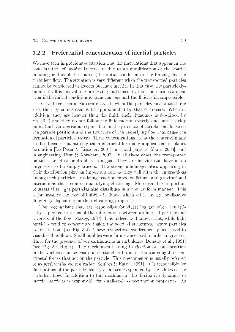
3.2 Con entration properties 393.2.2 Preferential on entration of inertial parti lesWe have seen in previous subse tion that the u tuations that appear in the on entration of passive tra ers are due to an ampli ation of the spatialinhomogeneities of the sour e (the initial ondition or the for ing) by theturbulent ow. The situation is very dierent when the transported parti les annot be onsidered as tra ers but have inertia. In that ase, the parti le dy-nami s itself is not volume-preserving and on entration u tuations appeareven if the initial ondition is homogeneous and the uid is in ompressible.As we have seen in Subse tion 3.1.1, when the parti les have a too largesize, their dynami s annot be approximated by that of tra ers. When inaddition, they are heavier than the uid, their dynami s is des ribed byEq. (3.2) and they do not follow the uid motion exa tly and have a delayon it. Su h an inertia is responsible for the presen e of orrelations betweenthe parti le positions and the stru ture of the underlying ow that ause theformation of parti le lusters. These on entrations are at the enter of manystudies be ause quantifying them is ru ial for many appli ations in planetformation [De Pater & Lissauer, 2001, in loud physi s [Shaw, 2003, andin engineering [Post & Abraham, 2002. In all these ases, the transportedparti les are dust or droplets in a gas. They are heavier and have a toolarge size to be simply tra ers. The strong inhomogeneities appearing intheir distribution play an important role as they will alter the intera tionsamong su h parti les. Modeling rea tion rates, ollisions, and gravitationalintera tions thus requires quantifying lustering. Moreover it is importantto stress that light parti les also distribute in a non uniform manner. Thisis for instan e the ase of bubbles in uids, whi h settle, merge, or dissolvedierently depending on their lustering properties.The me hanisms that are responsible for lustering are often heuristi- ally explained in terms of the intera tions between an inertial parti le anda vortex of the ow [Maxey, 1987. It is indeed well known that, while lightparti les tend to on entrate inside the vorti al stru tures, heavy parti lesare eje ted out (see Fig. 3.4). These properties have frequently been used tovisualize uid ows. Small bubbles were for instan e used in order to give evi-den e for the presen e of vortex laments in turbulen e [Douady et al., 1991(see Fig. 3.4 Right). The me hanism leading to eje tion or on entrationin the vorti es an be easily understood in terms of the entrifugal or en-tripetal for es that a t on the parti le. This phenomenon is usually referredto as preferential on entration [Squires & Eaton, 1991. It is responsible foru tuations of the parti le density at all s ales spanned by the eddies of theturbulent ow. In addition to this me hanism, the dissipative dynami s ofinertial parti les is responsible for small-s ale on entration properties. As

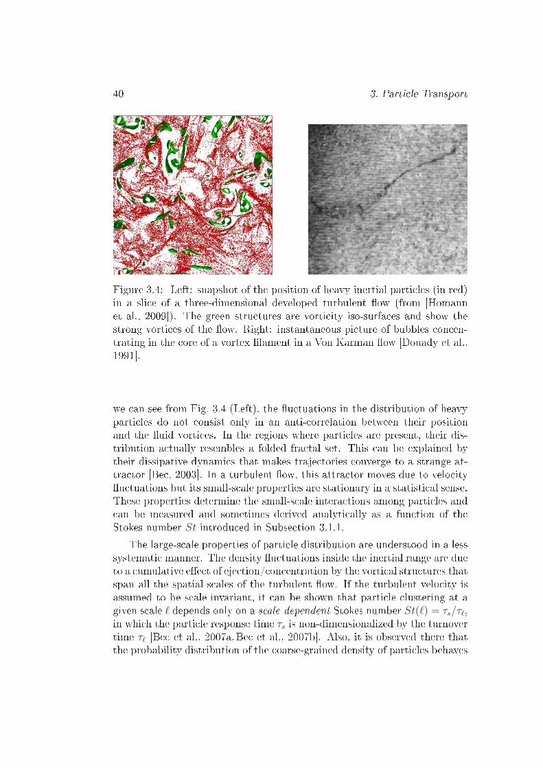
40 3. Parti le Transport

Figure 3.4: Left: snapshot of the position of heavy inertial parti les (in red)in a sli e of a three-dimensional developed turbulent ow (from [Homannet al., 2009). The green stru tures are vorti ity iso-surfa es and show thestrong vorti es of the ow. Right: instantaneous pi ture of bubbles on en-trating in the ore of a vortex lament in a Von Karman ow [Douady et al.,1991.we an see from Fig. 3.4 (Left), the u tuations in the distribution of heavyparti les do not onsist only in an anti- orrelation between their positionand the uid vorti es. In the regions where parti les are present, their dis-tribution a tually resembles a folded fra tal set. This an be explained bytheir dissipative dynami s that makes traje tories onverge to a strange at-tra tor [Be , 2003. In a turbulent ow, this attra tor moves due to velo ityu tuations but its small-s ale properties are stationary in a statisti al sense.These properties determine the small-s ale intera tions among parti les and an be measured and sometimes derived analyti ally as a fun tion of theStokes number St introdu ed in Subse tion 3.1.1.The large-s ale properties of parti le distribution are understood in a lesssystemati manner. The density u tuations inside the inertial range are dueto a umulative ee t of eje tion/ on entration by the vorti al stru tures thatspan all the spatial s ales of the turbulent ow. If the turbulent velo ity isassumed to be s ale-invariant, it an be shown that parti le lustering at agiven s ale ℓ depends only on a s ale-dependent Stokes number St(ℓ) = τs/τℓ,in whi h the parti le response time τs is non-dimensionalized by the turnovertime τℓ [Be et al., 2007a,Be et al., 2007b. Also, it is observed there thatthe probability distribution of the oarse-grained density of parti les behaves

3.2 Con entration properties 41as a power law at small values and has a tail fatter than Gaussian at largevalues. Su h properties are reprodu ed by simple mass eje tion models on alatti e [Be & Chétrite, 2007. As we will see in Chap. 6, a part of the workdeveloped in this thesis onsisted in extending this last work to settingswhere the rate at whi h parti les are eje ted depends ontinuously on spa eand time and displays s ale-invarian e properties.

42 3. Parti le Transport

Chapter 4Diusivity in turbulent pairdispersionRelative dispersion in a turbulent ow gives rise to a onsiderable interestsin e, as seen in previous hapter, it is one of the main key to des ribese ond-order statisti s in turbulent transport and mixing. It is importantto understand the physi al me hanisms behind pair dispersion in order toimprove the models used for instan e to predi t pollutant dispersion in theatmosphere as well as in the seas. The time evolution of the separation be-tween two tra er parti les was rst studied in [Ri hardson, 1926. Sin e then,mu h work has been devoted to understand the statisti s of pair dispersion(see for instan e [Bat helor, 1952,Krai hnan, 1966,Monin & Yaglom, 1971and for re ent reviews [Falkovi h et al., 2001,Sawford, 2001,Salazar & Collins,2009). However several questions remain today without a denite answer.For example, the dependen e on the initial separation of the probabilitydensity fun tion of the distan e between two parti les is still the matter ofsome debate [Bourgoin et al., 2006,Rast & Pinton, 2011,S atama hia et al.,2012. To address this issue, one has to onsider in addition to the initialseparation, the inuen e of the initial ondition of the velo ity and a elera-tion dieren es and to possibly identify dierent regimes of separation. This hapter reports thesis work on the time evolution of the mean square dis-tan e between two tra ers. This study is the subje t of an arti le publishedon Physi al Review E [Bitane et al., 2012b. The results of this study open theway to new possible explanations of the me hanisms leading to Ri hardsonObukhov law, whi h are an alternative to the ommonly-a epted s enariobased on a s ale-dependent ee tive diusivity.43

44 4. Diusivity in turbulent pair dispersion4.1 The regimes of tra er separationTurbulen e has the feature of strongly enhan ing the dispersion and mixingof the spe ies it transports. Also, as explained in Chap. 3, tra ers transportedby a turbulent ow approa h a diuse behavior on time s ales mu h longerthan the Lagrangian orrelation time of the ow [Taylor, 1921. These ideasare now ommonly used in appli ations, as for instan e in air quality ontrol,to model ee tive mixing properties in terms of an eddy diusivity. Su hmodels give a good handle on long-term averages and are su essfully usedto determine, for instan e, possible health hazards linked to a long exposuredownstream a pollutant sour e. However they are unable to apture stronglo al u tuations stemming from the omplex stru ture of the turbulent ow.Su h events annot be dire tly predi ted from the averaged on entrationeld as they relate to higher-order moments. A essing these u tuationsis ru ial in order to quantify for instan e the likeliness of nding a lo al on entration ex eeding a high threshold.As we have seen in Se . 3.2.1, se ond-order statisti s, su h as the varian eof a transported on entration eld and more generally the spatial orrelationof a passive s alar, are statisti ally related to the relative motion of tra ers. Inturbulen e, the distan e |R(t)| between two Lagrangian traje tories followsthe Ri hardsonObukhov superdiusive law〈|R(t)|2〉 ∼ ε t3, (4.1)where ε is the mean rate of kineti energy dissipation and the average isperformed over all the realizations. The long-term behavior of su h a sep-aration be omes independent of the initial separation |R(0)| = r0, when ethe designation of explosive pair separation. This superdiusive separationis mu h faster and less predi table than in any haoti system. Some in- ertitudes remain on the validity and the possible onvergen e to this law,be ause su h an explosive behavior is very arduous to observe both in nu-meri s and in experiments. This is basi ally due to the di ulty to havea huge s ale separation between the dissipative lengths, the initial separa-tion of tra ers, the observation range and the integral s ale of the ow (thereader an refer to [Sawford, 2001 and [Salazar & Collins, 2009 for reviewson that questions). Mu h eort has been devoted to test the universal-ity of this law, whi h was a tually retrieved in various turbulent settings,su h as the two-dimensional inverse as ade [Jullien et al., 1999,Boetta &Sokolov, 2002b, buoyan y-driven ows [S huma her, 2008, and magneto-hydrodynami s [Busse & Müller, 2008.

4.1 The regimes of tra er separation 454.1.1 Ri hardson's diusive approa hIn the ommonly a epted sense, studying turbulent relative dispersion on-sists in onsidering the evolution of the separationR(t) = X1(t)−X2(t) (4.2)between two tra ers X1(t) and X2(t). In these settings the initial distan e

r0 = |R(0)| is xed. Ri hardson's original arguments [Ri hardson, 1926 anbe reinterpreted by assuming that the velo ity dieren e V (t), dened asV (t) = u(X1, t)− u(X2, t), (4.3)between the two tra ers has a short orrelation time. This means that the entral-limit theorem applies and that, for su iently large times ales, onehas

dR

dt= V ≃

√

2 τL(R) U(R) ξ(t), (4.4)where ξ is the standard three-dimensional white noise, U is the Eulerianvelo ity dieren e orrelation tensor (su h that UTU = 〈δu ⊗ δu〉, whereδu is the Eulerian velo ity in rement omputed over a separation R= |R|),and τL the Lagrangian orrelation time of velo ity dieren es between pairseparated by R. Note that the produ t is here understood in the Stratonovi hsense. This formulation in terms of a sto hasti equation an equivalentlybe written for the two-point transition probability density p2(r, t|r0, 0) (seeSe . 3.1.2 for details on these notions). The density p2 is thus a solution tothe FokkerPlan k equation

∂tp2 = ∂ri[

τL UT U∂rjp2

]

, (4.5)where τL and U are evaluated at the separation r.As stressed in [Obukhov, 1941, when assuming Kolmogorov 1941 s alingwe an approximateτL ∼ r2/3, U ∼ r1/3, (4.6)where r = |r|. In addition, be ause of isotropy and when integrating overangles, the transition probability depends only on r and r0. The FokkerPlan k equation an then be rewritten as

∂tp2 =1

r2∂r

[

r2K(r) ∂rp2]

, (4.7)where K is the s ale-dependent diusivity of the separation diusive pro ess.For separations r within the inertial range of turbulen e one hasK(r) ∝ ε1/3r4/3. (4.8)

46 4. Diusivity in turbulent pair dispersionEquation (4.7) exa tly orresponds to that derived by Ri hardson for thetransition probability density p(r, t | r0, 0) at large timesp2(r, t | r0, 0) ∝

r2

〈|R(t)|2〉3/2 exp

[

− Ar2/3

〈|R(t)|2〉1/3]

, (4.9)where A is a positive onstant. The transition probability density is thusentirely determined by the se ond-order moment of the separation |R(t)|that, a ording to Eq.(4.7), is satisfying at large times〈|R(t)|2〉 ≃ g ǫ t3, (4.10)where g is a positive onstant (usually alled the Ri hardson onstant) relatedto A. The average is here taken over all pairs that are initially at a distan e

|R(0)| = r0.The key hypothesis in order to derive a FokkerPlan k equation of theform in Eq. (4.5) for the separation R is that velo ity dieren es V (t) be-tween tra ers are orrelated over times ales mu h smaller than those of inter-est, so that τL(r) ≪ t. As noti ed for instan e in [Falkovi h et al., 2001, thisassumption an hardly be invoked. It is indeed expe ted that the Lagrangianturnover time τL will be of the order of the orrelation for eddies of size r.It is known in turbulen e that su h eddies are orrelated over a time of theorder of their turnover time given byτr =

r

δru∼ ε−1/3r2/3. (4.11)Hen e for separations that, a ording to Eq. (4.10), grow like r ∼ (εt3)1/2,one has τL ∼ τr ∼ t, so that the dominant ow stru tures in the separationdynami s are in prin iple orrelated over times ales of the order of the obser-vation time. This implies that the entral limit theorem annot be appliedand that the approximation in Eq. (4.4) does not hold. This is an issue injustifying the sto hasti approa h that we have just mentioned.Despite su h short omings, the diusive approa h proposed by Ri hard-son and in parti ular the expli it form in Eq. (4.9) for the transition prob-ability density, have proven being relevant in some asymptoti s [Ott &Mann, 2000, Biferale et al., 2005, Ouellette et al., 2006, Salazar & Collins,2009,Eyink, 2011. Also, mu h work on relative dispersion has used it as abasis. For instan e, improvements of Eq. (4.9) were proposed using modiedversions of the eddy diusivity K(r), adding a time dependen e [Bat helor,1952,Krai hnan, 1966 or, more re ently, in luding nite Reynolds numberee ts [S atama hia et al., 2012. All of these improvements strongly alterthe fun tional form of the large-r tail of the transition probability density.

4.1 The regimes of tra er separation 47Nevertheless, the physi al me hanisms leading to the de- orrelation of ve-lo ity dieren es and to models based on eddy diusivity are still un learand many questions remain open. In this hapter, we mainly fo us on theme hanisms that justify a onvergen e to the Ri hardsonObukhov law. Inparti ular we address the questions of the speed at whi h su h a onvergen eo urs and of the form of subleading terms, whi h is still not known. Inthis light, we will ome ba k in next hapter on the problem of the formof the transition probability density, with a fo us on the me hanisms givingextreme u tuations.4.1.2 Bat helor's ballisti regimeThe rst work dealing with the way pair separation onverges to the Ri hard-son superdiusive behavior is due to G.K. Bat helor [Bat helor, 1950. Heargued that the explosive t3 law is pre eded by a ballisti phase during whi hthe tra ers keep their initial velo ity and separate as〈|R(t)−R(0)|2〉 ≃ t2S2(r0), (4.12)where S2(r) = 〈|δru|2〉 is the Eulerian se ond-order stru ture fun tion overa separation r, omputed with absolute values. This regime holds till a times ale that is a fun tion of the initial separation r0, known as Bat helor'stime [Biferale et al., 2005,Bourgoin et al., 2006tB(r0) = τr0 ∼ ε−1/3r

2/30 , (4.13)whi h is equal to the eddy turnover time asso iated to the initial separa-tion r0. After this time, there is a transition to the Ri hardson regime andthe dynami s loses all memory on the initial ondition. In this Bat helor±regime, the velo ity remains strongly orrelated, so that it an learly not bedes ribed by an eddy-diusivity approa h.Various sto hasti models have been designed to at h both Bat helor'sand Ri hardson's regimes. Most of them are based on the observation thatthe a eleration dieren e between the two tra ers is shortly orrelated butthey do not assume that velo ity dieren es get un orrelated. The pairseparation and the velo ity dieren e an then be approximated as oupledMarkovian diusive pro esses (see [Kurbanmuradov, 1997,Sawford, 2001 forreviews). The usual path for designing su h models requires imposing some onstraints on the drift and the diusion terms. Thomson argued that theyshould satisfy the well-mixed ondition [Thomson, 1987: when averagingover uniformly separated pairs inside the whole inertial range, the statisti s

48 4. Diusivity in turbulent pair dispersionof velo ity dieren es between the two tra ers has to re over Eulerian two-point statisti s. Denitively, devising an admissible model requires an inputfrom Eulerian statisti s [Borgas & Yeung, 2004. We have seen in Chap. 2that, in turbulen e, the distribution of velo ity dieren es is neither self-similar nor Gaussian. Be ause of that, su h models be ome so ompli atedthat they an hardly be used to improve the understanding of the underlyingphenomenology and, at the same time, they are not easily amenable for ananalyti al treatment.To larify when and where Ri hardson's approa h might be valid, it isimportant to understand the times ale of onvergen e to the explosive t3law. Mu h work has re ently been devoted to this issue: it was for instan eproposed to make use of fra tional diusion with memory [Ilyin et al., 2010,to introdu e random delay times of onvergen e to Ri hardson s aling [Rast& Pinton, 2011, or to estimate the inuen e of extreme events in parti leseparation [S atama hia et al., 2012. The last point will be studied indetail in the next hapter. All these approa hes onsider as granted that thenal behavior of separations is given by Ri hardson's diusive approa h. Aswe will see here, many aspe ts of the onvergen e to Ri hardson's law forpair dispersion an be laried in terms of a diusive behavior of velo itydieren es.4.2 Times ales of two-parti le dispersionWe fo us in this se tion on determining the various times ales that are in-volved in the problem of tra er relative dispersion.4.2.1 Settings of the numeri al simulationsTo investigate su h issues, we have used the data from dire t numeri al simu-lations of the in ompressible NavierStokes equation in the three-dimensional2π-periodi domain. These simulations were performed with the ode LaTudeveloped by H. Homann [Homann et al., 2007. This ode uses a standardpseudo-Fourier-spe tral solver for al ulating the spatial derivatives in thevarious terms of NavierStokes equation, together with a third-order RungeKutta s heme for the temporal evolution. Su h a method is well adaptedto in ompressible homogeneous and isotropi turbulen e at high Reynoldsnumbers with an extended inertial range of s ales. It has the advantages of ombining a high degree of a ura y with very good performan es on mas-sive parallel super omputers su h as BlueGene systems and large Intel/AMD

4.2 Times ales of two-parti le dispersion 49Table 4.1: Parameters of the numeri al simulationsN Rλ δx δt ν ε urms η τη L τL

20483

460 3.7·10−36·10−4

2.5·10−53.6·10−3

0.19 1.4·10−30.083 1.85 9.9

40963

730 1.53·10−31.2·10−3

1.0·10−53.8·10−3

0.19 7.2·10−40.05 1.85 9.6

N is the number of grid points, Rλ the Taylor-based Reynolds number, δxthe grid spa ing, δt the time step, ν the kinemati vis osity, ε the averagedenergy dissipation rate, urms the root-mean square velo ity, η=(ν3/ε)1/4 theKolmogorov dissipative s ale, τη = (ν/ε)1/2 the asso iated turnover time,L = u3

rms/ε the integral s ale and τL = L/urms the asso iated large-s aleturnover time. lusters. One of the main advantages of the ode LaTu is that it uses apen il representation of the domain. While traditionally in pseudo-spe tral odes the domain is divided in two-dimensional slabs, a de omposition inone-dimensional elements is here used. This allows one to use a maximumnumber of pro essors, whi h is given by the square number of grid-points inone dire tion, instead of this number itself when using slab de ompositions.For instan e, while in a 10243 simulation traditional odes an usually use amaximum of 1024 pro esses where two-dimensional fast Fourier transformsare performed, the ode LaTu an use up to 10242 pro esses in whi h one-dimensional transforms are arried out. The ode is parallelized using MPIand, be ause of its pen il representation of the domain, an run on massivelyparallel omputers using up to several tens of thousands pro essors.We have used two sets of simulations whose parameters are summarized inTable 4.1 (more details on these spe i simulations an be found in [Graueret al., 2012). In both simulations, the resolution is su h that kmax η =(N/3) η ≈ 1. As we are interested in inertial-range quantities, we do notneed a very high resolution of the dissipative s ales. To maintain a statisti alsteady state, the ow is for ed by keeping onstant the energy ontent of thetwo rst shells of wavenumbers in Fourier spa e. This implies that in bothsimulations the for ing s ale is Lf = π. The Eulerian se ond-order stru turefun tion measured from these two simulations are represented in Fig. 4.1.As seen there, the largest one develops a signi ant s aling range wheredeviations from Kolmogorov 1941 s aling start to be visible. For ea h valueof the Reynolds number, the ow is seeded with 107 tra er parti les whosemotion is integrated using tri-linear interpolation. Positions, velo ities, anda elerations of tra ers have been stored with enough frequen y for studying

50 4. Diusivity in turbulent pair dispersion

100

101

102

103

104

100

101

102

103

104

r / η

S 2(r)

/ uη2

R

λ = 730

Rλ = 460

Figure 4.1: Se ond-order Eulerian absolute-value stru ture fun tion S2(r) =〈|u(x + r, t) − u(x, t)|2〉 for the two values of the Reynolds number inves-tigated in this thesis. The dashed line represents Kolmogorov 1941 s alingS2(r) ≃ (11/3)C2(ε r)

2/3 with C2 = 2.13. The solid line orresponds to She-Lévêque anomalous s aling with ζ2 ≈ 0.696 (see [She & Lévêque, 1994). Theverti al and horizontal olored dashed lines indi ate the integral s ale L andthe large-s ale velo ity, respe tively.relative motion. These simulations were performed on the BlueGene ma hineJuGene of the German omputer Center of Jüli h in the framework of theXXL proje t HBO28. They required more than ten millions of CPU hours.All the statisti al studies reported in this hapter and in the next one havebeen done using these datasets.To provide a rst insight on the numeri al simulations that we have usedand on the typi al values of the times ales and lengths ales that are usedthroughout this and next hapter, let us shortly report some measurements onrelative dispersion. One of the major di ulties en ountered when approa h-ing numeri ally this problem is that it requires a huge times ale separation.Indeed, to observe Ri hardsonObukhov t3 superdiusive regime, one needsat least to follow parti le pairs on a time t mu h longer than the Kolmogorovdissipative time τη = (ν/ǫ)1/2 and mu h shorter than the eddy turnover timeτL asso iated to the integral s ale L. Also, in order to observe possibly uni-versal me hanisms of onvergen e to Ri hardson's explosive behavior, it is inprin iple required that the initial distan e r0 belongs to the inertial range. Inparti ular, a possible proper res aling in terms of r0 of transients to the t3 law

4.2 Times ales of two-parti le dispersion 51

10−1

100

101

102

103

100

102

104

106

108

t / τη

<|R

(t)|2 >

/ η2

(a) Rλ = 730

L2

τL

10−1

100

101

102

103

100

102

104

106

108

t / τη

<|R

(t)|2 >

/ η2

(b) Rλ = 460

L2

τL

r0 = 2η

r0 = 3η

r0 = 4η

r0 = 6η

r0 = 8η

r0 = 12η

r0 = 16η

r0 = 24ηFigure 4.2: Time-evolution of the mean-squared distan e for Rλ = 730 (a)and Rλ = 460 (b) for various initial separations r0 as labeled. The horizon-tal and verti al solid lines represent the integral s ale L and its asso iatedturnover time τL, respe tively. The dashed line orresponds to the explosiveRi hardson-Obukhov law given by Eq. (4.10) with g = 0.52. an only be valid if the observation time t is mu h longer than the turnovertime τr0 ∼ ε−1/3r

2/30 asso iated to the initial separation |R(0)| = r0, whi hitself has to be longer than τη. We should thus have τη ≪ τr0 ≪ t ≪ τL.To give a on rete idea, if we require that these times ales are separated byat least a de ade, this implies that one should have a Taylor-based Reynoldsnumber Rλ =

√15 (τL/τη) & 4000. Su h a high level of turbulen e is stillfar from present-day experimental setups where a urate parti le tra kingte hniques an be used (see [Salazar & Collins, 2009,Tos hi & Bodens hatz,2009 for re ent reviews). Also, su h large values of the Reynolds number areunrea hable by state-of-the-art dire t numeri al simulations. At the momentthere is no simulations of lagrangian tra ers in homogeneous isotropi turbu-len e with more than 40963 grid points. As we have seen in Table. 4.1, withsu h a resolution, we have attained Rλ = 730 as it was de ided to resolvewell the dissipative s ales. De reasing su h a pre ision an help in rea hingat maximum Rλ ≈ 1100, with the risk of missing violent small-s ale intermit-tent stru tures [Ishihara et al., 2009. For this reason, there is an importantneed for understanding the full pro ess of onvergen e to the t3 law in orderto predi t and dete t for instan e possible subleading orre tions. This is thespirit whereby this thesis work is presented.After a time su iently long to have onverged to a statisti al steadystate (around one large-s ale turnover time), we start the analysis of thedispersion of tra er pairs. For this, we label at a xed initial time (that weset here to be t = 0) all ouples whose distan e |R(0)| = |X1(0) − X2(0)|

52 4. Diusivity in turbulent pair dispersionis equal to r0 ± η for r0 ≤ 16 η and equal to r0 (1 ± 2%) for r0 > 16 η withr0 = 2, 3, 4, 6, 8, 12, 16, 24, 32, 48, 64, 96, 128, and 192η. This bining was ho-sen su h that ea h family indexed by r0 ontains a few hundreds of thousandsof pairs. We then tra k forward in time all indexed pairs and perform statis-ti s onditioned on their initial separation r0. Figure 4.2 shows for the twosimulations the time evolution of the mean squared distan e 〈|R(t)|2〉 for var-ious values of the initial separation r0. Time and spa e are there representedin dissipative-s ale units. After a transient (whi h roughly orresponds toBat helor's ballisti regime), the mean-squared distan e approa hes the ex-plosive Ri hardsonObukhov regime 〈|R(t)|2〉 ≃ g ε t3 written in Eq. (4.10).We observe for both values of the Reynolds number a Ri hardsonObukhov onstant g ≈ 0.52 ± 0.05. In the next two subse tions, we will see how to hara terize the time at whi h the onvergen e to this regime o urs.4.2.2 Times ale of departure from Bat helor's regimeAs already motivated in Se . 4.1, the obje tive is here to understand betterthe times ale at whi h the average separation between tra ers onverges tothe t3 Ri hardson s aling observed in previous subse tion. Let us beginwith rewriting the initial ballisti behavior Eq. (4.12) of the average squaredseparation, together with its subleading term. For that we follow the samealgebrai steps as in [Ouellette et al., 2006. A Taylor expansion at shorttimes of the separation leads to

⟨

|R(t)−R(0)|2⟩

r0= t2〈|δr0u|2〉+ t3 〈δr0u · δr0a〉+O(t4). (4.14)We have here denoted by 〈·〉r0 the average over all tra er pairs that are ini-tially at a distan e r0 from ea h other. This notation is useful to distinguishthis Lagrangian average from the Eulerian average, whi h is denoted by thesimple bra kets 〈·〉. We have also used δru to designate the Eulerian in re-ment u(x+r, t)−u(x, t), where r = |r|. Finally, δra is the Eulerian in rementof the uid a eleration, dened as δra = [∂tu+ u · ∇u](x+ r, t)− [∂tu+u ·

∇u](x, t).As long as the rst term (proportional to t2) in the right-hand side ofEq. (4.14) is dominant, the tra ers separate ballisti ally. Clearly the expan-sion fails when the se ond subleading term in the right-hand side be omesof the same order as that giving the ballisti separation. This happens whenthe time is of the order oft ≈ t0 =

S2(r0)

| 〈δr0u · δr0a〉 | , where S2(r0) = 〈|δr0u|2〉. (4.15)

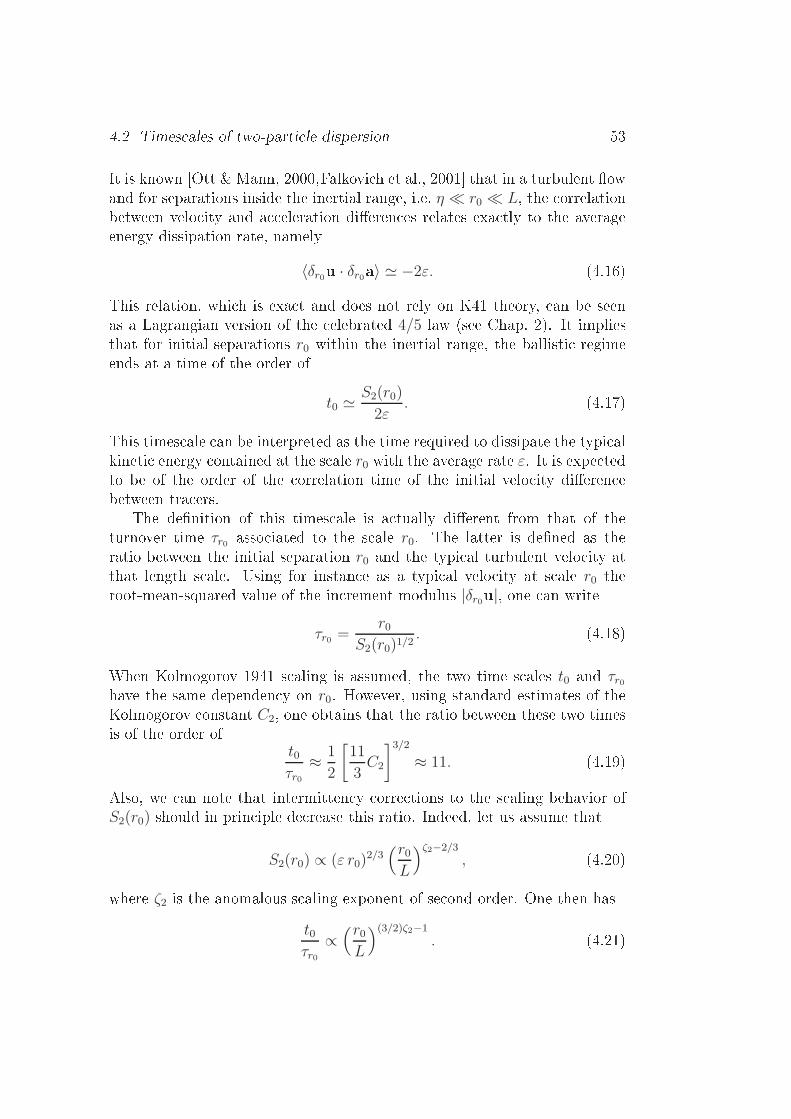
4.2 Times ales of two-parti le dispersion 53It is known [Ott & Mann, 2000,Falkovi h et al., 2001 that in a turbulent owand for separations inside the inertial range, i.e. η ≪ r0 ≪ L, the orrelationbetween velo ity and a eleration dieren es relates exa tly to the averageenergy dissipation rate, namely〈δr0u · δr0a〉 ≃ −2ε. (4.16)This relation, whi h is exa t and does not rely on K41 theory, an be seenas a Lagrangian version of the elebrated 4/5 law (see Chap. 2). It impliesthat for initial separations r0 within the inertial range, the ballisti regimeends at a time of the order of

t0 ≃S2(r0)

2ε. (4.17)This times ale an be interpreted as the time required to dissipate the typi alkineti energy ontained at the s ale r0 with the average rate ε. It is expe tedto be of the order of the orrelation time of the initial velo ity dieren ebetween tra ers.The denition of this times ale is a tually dierent from that of theturnover time τr0 asso iated to the s ale r0. The latter is dened as theratio between the initial separation r0 and the typi al turbulent velo ity atthat length s ale. Using for instan e as a typi al velo ity at s ale r0 theroot-mean-squared value of the in rement modulus |δr0u|, one an write

τr0 =r0

S2(r0)1/2. (4.18)When Kolmogorov 1941 s aling is assumed, the two time s ales t0 and τr0have the same dependen y on r0. However, using standard estimates of theKolmogorov onstant C2, one obtains that the ratio between these two timesis of the order of

t0τr0

≈ 1

2

[

11

3C2

]3/2

≈ 11. (4.19)Also, we an note that intermitten y orre tions to the s aling behavior ofS2(r0) should in prin iple de rease this ratio. Indeed, let us assume that

S2(r0) ∝ (ε r0)2/3

(r0L

)ζ2−2/3

, (4.20)where ζ2 is the anomalous s aling exponent of se ond order. One then hast0τr0

∝(r0L

)(3/2)ζ2−1

. (4.21)

54 4. Diusivity in turbulent pair dispersion

100

101

102

103

100

101

102

103

r0/η

t 0/τ η

t0 = τL

r0 = L

Figure 4.3: Dissipation time t0 as a fun tion of r0 in dissipative-s ale units.Here the blue solid line is obtained by Eulerian averages, while the green ross marks are the a tual Lagrangian measurements. The red dashed lineshows the turnover time τ(r0) = r0/[S2(r0)]1/2. Here and in the sequel wehave used the Lagrangian data to estimate se ond-order stru ture fun tion

S2(r0) and t0. The two verti al and horizontal dotted lines show the larges ale L and its asso iated turnover time τL (obtained from K41).We know from experimental and numeri al measurements in turbulent ows(see, e.g., Fig. 4.1), that ζ2 ≈ 0.7 > 2/3. This implies that the ratio betweenthe dissipation time t0 and the turnover time in Eq. (4.21) in reases as afun tion of r0.The two times ales are shown in Fig. 4.3 for the simulation with Rλ = 730(N = 40963 grid points). One learly sees a dis repan y between the twodenitions. This dieren e in reases when r0 in reases and de reases at s alesof the order of the integral s ale L. In the sequel, to measure t0 as a fun tionof r0, we have not used its Eulerian estimate but rather a Lagrangian averagewhere the se ond-order stru ture fun tion S2(r0) is obtained by taking themean of δu over all pairs that are labeled at a distan e r0.Turning ba k to our al ulation of the subleading terms in Bat helor'sballisti regimes, we introdu e in Eq. (4.14) the time s ale t0. For times tmu h smaller than t0, we an then write⟨

|R(t)−R(0)|2⟩

r0= t20 S2(r0)

[

t

t0

]2 [

1− t

t0

]

+ h.o.t., (4.22)where h.o.t. stands for higher-order terms. Figure (4.4) shows the time evo-

4.2 Times ales of two-parti le dispersion 55

10−3

10−2

10−1

100

101

102

10−6

10−3

100

103

106

t/t0

〈|R

(t)−

R(0

)|2〉 r

0/

[t2 0S

2(r

0)]

r0 = 2ηr0 = 3ηr0 = 4ηr0 = 6ηr0 = 8ηr0 = 12ηr0 = 16ηr0 = 24ηr0 = 32ηr0 = 48η

Figure 4.4: Res aled mean-square separation between two traje tories asa fun tion of time for Rλ = 730 and dierent initial separations r0. Thedashed line represents the two leading terms of the ballisti behavior (4.22).The solid line is a t to the Ri hardson's regime, Eq. (4.23), with g = 0.525and C = 2.5.lution of the mean-squared displa ement for various values of the initial sep-aration r0. Here and in the sequel the gures are shown for Rλ = 730, unlessspe ied. It is learly visible that, on e that the time t has been res aled byt0 and the squared distan es by t20 S2(r0), all measurements ollapse almostperfe tly onto a single urve when r0 is far enough in the inertial range. Fur-ther, data are in rather good agreement with the departure from the ballisti regime predi ted by Eq. (4.22).4.2.3 Convergen e to the super-diusive behaviorIt is important to note that the data ollapse observed in Fig. 4.4 extends totimes larger than t0 when the mean squared separation tends to Ri hardsont3 regime. Su h unexpe ted fa t implies that t0 is not only the times ale ofdeparture from the ballisti regime, but also that of onvergen e to Ri hard-son's law. In parti ular, numeri al data suggest that the large-time behaviortakes the form

⟨

|R(t)−R(0)|2⟩

r0= g ε t3

[

1 + Ct0t

]

+ h.o.t. (4.23)

56 4. Diusivity in turbulent pair dispersion

10−2

10−1

100

101

102

100

101

102

t / t0

<|R

(t)−

R(0

)|2 > /

(ε t3 )

(a)r0 = 4η

r0 = 6η

r0 = 8η

r0 = 12η

r0 = 16η

r0 = 24η

Figure 4.5: Compensated mean-squared displa ement 〈|R(t)−R(0)|2〉/(ε t3)as a fun tion of t/t0, with t0 = S2(r0)/(2ε), for various initial separations andRλ = 730 () and Rλ = 460 (+). The two urves show behaviors of the form〈|R(t)−R(0)|2〉 ≃ g ε t3+A t2, with A = S2(r0), given by Bat helor's ballisti regime (bla k dotted line), and A = 2.5 g /t20 (grey dashed line).The term C appearing here does not strongly depend on the Reynolds numberand a tually, for both values of the Reynolds number, we obtain the sameresults, up to statisti al errors. This is eviden ed in Fig. 4.5, whi h shows the ompensated mean squared in rease of the distan e 〈|R(t) − R(0)|2〉/(ε t3)for the two investigated values of the Reynolds number. In this gure, thetime has been again res aled by t0 = S2(r0)/(2ε). Data onrm that thesubdominant terms in Ri hardson explosive regime are ∝ t2, as postulatedin Eq. (4.23). One also observes that the onstant C is independent of r0when r0 ≫ η. The subleading terms, appearing at large times from the ompensated plot in Fig. 4.5, are learly dierent from those oming from asubleading ballisti regime. We indeed see on the gure that the two bla klines do not oin ide. The dotted line, whi h orresponds to Bat helor'sregime, gives a good approximation to the data up to a few hundredth oft0. On the ontrary, the dashed line orresponds to the proposed formula ofEq. (4.23) with C ≈ 2.5 and is valid only for t ≫ t0.Systemati measurements of the onstant C as a fun tion of the initialseparations have been performed and are shown in Fig. 4.6. This was done

4.2 Times ales of two-parti le dispersion 57

100

101

102

−8

−6

−4

−2

0

2

4

r0 / η

g C

(b)

Rλ = 730

Rλ = 460Figure 4.6: Measured value of the onstant g C in front of the subleadingterm as a fun tion of the initial separation. It stabilizes to C ≈ 1.3/g ≈ 2.5for r0 ≫ η; this value is represented as a dashed line.by estimating numeri ally the produ t of the onstants g and C in the om-pensated mean-squared displa ement. We nd that C is negative when r0is of the order of the Kolmogorov s ale η. In this ase, the onvergen e tothe Ri hardson law o urs from below and it is thus ontaminated by tra erpairs that spend long times lose together before sampling the inertial range.This is also onsistent with the re ent ndings of [S atama hia et al., 2012.The onvergen e to Ri hardson's law from below for su h values of r0 leadsto an intermediate time range where the mean squared distan e grows evenfaster than the explosive t3 law, as for instan e observed in [Biferale et al.,2005. When r0 is instead far-enough in the inertial range (r0 & 8η), we ndthat C ≈ 1.3/g ≈ 2.5 be omes independent on the initial separation and, onthe ontrary, the onvergen e to Ri hardson law is from above. Moreover,when the initial separation r0 approximates the value of 4η we have that C =0, independently of the Reynolds number. The only subleading terms presentin Eq. (4.23) are then of lower order (i.e. ∝ t instead of t2). As a onsequen e,the mean-squared separation onverges mu h faster to the Ri hardson regimefor su h an initial separation than for others. This observation indi ates thatthe initial separation r0 ≈ 4η ould be an optimal hoi e for hoosing setupsin order to observe the t3 behavior in experiments. However, su h smallvalues of r0 are learly not representative of the inertial-range behavior. We an note in Fig. 4.6 that the overlap between the onstants C obtained fromthe two values of Reynolds number is not observed for r0 = 4η. As in that

58 4. Diusivity in turbulent pair dispersion ase C is very small, this is ertainly due to the fa t that the tting form usedthere eases to give a good representation of the data. A better estimate ofC would require a ounting for next-order subleading terms.4.3 Statisti s of velo ity dieren es4.3.1 A diusive behavior?In this se tion, we are interested in the behavior of the velo ity dieren eV (t) = u(X1(t), t) − u(X2(t), t) between two tra ers as a fun tion of time.Ri hardson's t3 law for separations implies that the mean-squared velo itydieren es should behave at large times as

〈|V (t)|2〉r0 ≃ h ǫ t, (4.24)where h is a positive onstant that annot be straightforwardly expressedas a fun tion of the Ri hardson onstant g that appears in Eq. (4.10). Aswe have seen in Chap. 3, a behavior ∝ t of a mean-square quantity is a keyfeature of purely diusive sto hasti pro esses. In the rest of this hapter, wegive some eviden e that the large-time velo ity dieren e between two tra ers an indeed be understood as a diusion. Before presenting our argumentsfor that, we report the results of numeri al simulations on this quantity.Initially, the statisti s of V (0) are exa tly given by the Eulerian statisti sof velo ity in rements at a separation r0. We have used su h an argumentto derive the ballisti regime behavior of Eq. (4.14). At large times, thebehavior is expe ted to be given by Eq. (4.24). A naive pi ture would onsistin interpolating between these two behaviors by assuming that〈|V (t)|2〉r0 ≃ S2(r0) + h ǫ t. (4.25)Assuming su h a form, it an be expe ted that one of the two regimes isdominant when t is mu h smaller or mu h longer than t0 = S2(r0)/(2 ǫ). Asseen from Fig. 4.7 su h a form with h = 2.4 (represented as a dashed line)seems to be a good rst-order approximation. However, this pi ture is not ompletely satisfa tory. When zooming loser to the initial times (see inset),one observes that the averaged pair kineti energy 〈|V (t)|2〉r0 rst starts byde reasing for a time of the order of a few tens of t0. We indeed know thatinitially

V (t) = V (0) + tA(0) +O(t2), (4.26)where A(0) = (∂tu+u ·∇u)(X1(0), 0)− (∂tu+u ·∇u)(X2(0), 0) denotes theinitial dieren e of uid a eleration between the two tra er positions. This

4.3 Statisti s of velo ity dieren es 59

10−3

10−2

10−1

100

101

102

10−1

100

101

102

103

t / t0

<|V

(t)|2 >

/ S 2(r

0)

r0 = 2η

r0 = 3η

r0 = 4η

r0 = 6η

r0 = 8η

r0 = 12η

r0 = 16η

r0 = 24η

10−2

100

0.8

1

1.2

Figure 4.7: Time behavior of the mean-squared velo ity dieren e 〈|V (t)|2〉r0for Rλ = 730. It is here normalized by its initial value and represented as afun tion of the res aled time t/t0. The gray dashed line is the behavior givenby Eq. (4.24) of the form 〈|V (t)|2〉r0 ≃ S2(r0) + h ε t with h = 2.4. Inset:same but zoomed at short times; the bla k dotted line is the initial de reaseasso iated to kineti energy dissipation: 〈|V (t)|2〉r0 ≃ S2(r0)− 4 ε t.approximation leads to〈|V (t)|2〉r0 ≃ S2(r0)− 4 ǫ t. (4.27)A ording to our numeri al data, this regime seems to reprodu e well whatis happening for times up to ≈ 0.01 t0see inset of Fig. 4.7. The fa t thatthis predi tion eases to des ribe the data after su h a short times ale (thatis signi antly smaller than t0 instead of being of its order) indi ates thatthe subleading terms in Eq. (4.26) be ome important. As a onsequen e,depending on the quantity we are interested in, Bat helor's ballisti regimemight end very qui kly.After this subtle initial de rease, the averaged squared velo ity dieren eamplitude tends asymptoti ally to a behavior ∝ t. However this pro esso urs in a noti eably dierent manner to that of onvergen e of squaredseparation to Ri hardson t3 law: irrespe tive of the initial separation r0, thequantity 〈|V (t)|2〉r0 always approa hes from below the asymptoti behavior.In other terms, we observe that for a xed value of t/t0, the pair kineti energy 〈|V (t)|2〉r0 is an in reasing fun tion of r0/η and seems to onverge tothe behavior given in Eq. (4.24) only in the limit r0/η → ∞.

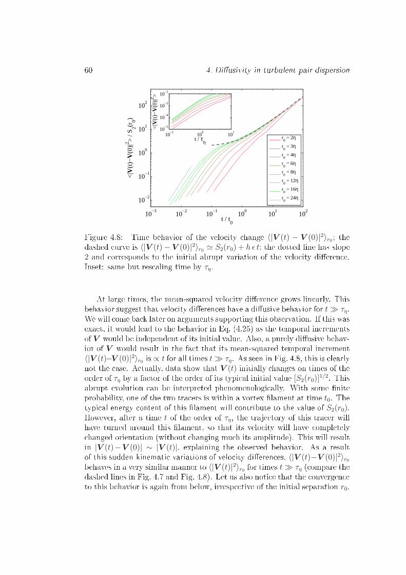
60 4. Diusivity in turbulent pair dispersion

10−3

10−2

10−1

100

101

102

10−2

10−1

100

101

102

t / t0

<|V

(t)−

V(0

)|2 > /

S 2(r0)

r0 = 2η

r0 = 3η

r0 = 4η

r0 = 6η

r0 = 8η

r0 = 12η

r0 = 16η

r0 = 24η

10−1

100

101

10−5

10−4

10−3

10−2

t / τη

<|V

(t)−

V(0

)|2 >

Figure 4.8: Time behavior of the velo ity hange 〈|V (t) − V (0)|2〉r0; thedashed urve is 〈|V (t)−V (0)|2〉r0 ≃ S2(r0) + h ǫ t; the dotted line has slope2 and orresponds to the initial abrupt variation of the velo ity dieren e.Inset: same but res aling time by τη.At large times, the mean-squared velo ity dieren e grows linearly. Thisbehavior suggest that velo ity dieren es have a diusive behavior for t ≫ τη.We will ome ba k later on arguments supporting this observation. If this wasexa t, it would lead to the behavior in Eq. (4.25) as the temporal in rementsof V would be independent of its initial value. Also, a purely diusive behav-ior of V would result in the fa t that its mean-squared temporal in rement〈|V (t)−V (0)|2〉r0 is ∝ t for all times t ≫ τη. As seen in Fig. 4.8, this is learlynot the ase. A tually, data show that V (t) initially hanges on times of theorder of τη by a fa tor of the order of its typi al initial value [S2(r0)]

1/2. Thisabrupt evolution an be interpreted phenomenologi ally. With some niteprobability, one of the two tra ers is within a vortex lament at time t0. Thetypi al energy ontent of this lament will ontribute to the value of S2(r0).However, after a time t of the order of τη, the traje tory of this tra er willhave turned around this lament, so that its velo ity will have ompletely hanged orientation (without hanging mu h its amplitude). This will resultin |V (t)−V (0)| ∼ |V (t)|, explaining the observed behavior. As a resultof this sudden kinemati variations of velo ity dieren es, 〈|V (t)−V (0)|2〉r0behaves in a very similar manner to 〈|V (t)|2〉r0 for times t ≫ τη ( ompare thedashed lines in Fig. 4.7 and Fig. 4.8). Let us also noti e that the onvergen eto this behavior is again from below, irrespe tive of the initial separation r0.

4.3 Statisti s of velo ity dieren es 61There is hen e an abrupt hange (o urring on times ales of the order ofτη) that prevent from determining an ee tive initial velo ity dieren e andthus from observing a lear diusive behavior of V (t). However, data suggestthat the times ale of onvergen e to this behavior is, as for separations, of theorder of t0. To understand further this question, we next turn to investigatingthe behavior of the longitudinal velo ity dieren e between the tra ers.4.3.2 Geometry of longitudinal velo itiesWe are here interested in the evolution of the longitudinal omponent V ‖(t) =R(t) ·V (t)/|R(t)| of the velo ity dieren e as a fun tion of time. This quan-tity is important to hara terize pair separation as d|R|/dt = V ‖. Initially,the averaged longitudinal velo ity vanishes, i.e. 〈V ‖(0)〉r0 = 0; this is due tothe statisti al stationarity of the uid ow. For times t ≪ t0 in the Bat h-elor's ballisti regime, the pairs are keeping their initial velo ity dieren eand one an easily he k that

〈V ‖(t)〉r0 ≃ t〈|V ⊥(0)|2〉r0

r0, (4.28)where V ⊥ denotes the omponents of V that are transverse to R. It is thus lear that the average velo ity at whi h tra er traje tories separate immedi-ately be omes positive. Figure 4.9, whi h represents the time evolution of

〈V ‖(t)〉r0, shows without doubt this initial linear growth.This in rease of the longitudinal velo ity dieren e has an interestinggeometri al interpretation. If all pairs were to maintain indenitely theirinitial velo ity dieren es V (0), it is lear that they would eventually allseparate at large times. Indeed, they will rea h a minimal distan e at anite timet∗ = − [R(0)·V (0)]

|V (0)|2 = − r0V‖(0)

|V (0)|2 , (4.29)whi h is positive for parti les that are initially approa hing. After su h timet∗, the distan e between parti les in reases and V ‖ be omes positive. Thisleads to an in rease of 〈V ‖〉r0 that omes from kinemati onsiderations andis obviously not due to any dynami s imposed by the turbulent ow. To esti-mate the typi al value of the minimal distan e at time t∗, we have performedstatisti s on pair separation onditioned not only on the initial distan e r0,but also on the initial longitudinal velo ity dieren e by binning pairs withV ‖(0) = v0 ± δv0. From these statisti s we have dened the averaged timet∗ = −r0v0/〈|V (0)|2 | v0〉r0 at whi h traje tories, with a given initial longitu-dinal velo ity dieren e v0, are at a minimal distan e. The data are shown in

62 4. Diusivity in turbulent pair dispersion

10−3

10−2

10−1

100

101

102

10−2

10−1

100

101

t / t0

< V

// (t)

> /

[S2(r

0)]1/

2

r0 = 4η

r0 = 6η

r0 = 8η

r0 = 12η

r0 = 16η

r0 = 24η

r0 = 32η

r0 = 48η

r0 = 64η

r0 = 96η

r0 = 128η

r0 = 192ηFigure 4.9: Time evolution of the averaged longitudinal velo ity dieren e

〈V ‖(t)〉r0 for various initial separations, as labeled, and for Rλ = 730. Thedashed line to the left has slope 1 and the dashed line to the right has a slope1/2.Fig. 4.10 for various values of r0 and as a fun tion of v0. We observe that forr0 ≫ η this time approximatively takes the form t∗ ≃ t0 f(v0/〈|V (0)|2〉1/2r0 ),where the fun tion f(x) attains its maximum (roughly equal to 0.05) atx ≈ 1. This onrms the observation made in Fig. 4.9 that the initial growthof 〈V ‖〉r0 o urs on a time length of the order of a few hundredths of t0.In addition to the hange in the mean longitudinal velo ity dieren e dis- ussed above, numeri al measurements show that the full distribution of V ‖loses its symmetry and develops fatter tails when time in reases. Figures 4.11and 4.12 represent the skewness S and the atness F of V ‖ as a fun tion oftime and for the same initial separations as in Fig. 4.9. These observables arefrequently used in turbulen e to quantify the shape of the velo ity in rementdistribution. For two-parti le Lagrangian statisti s, they are dened asS(t) =

⟨

[V ‖(t)− 〈V ‖(t)〉r0]3⟩

r0

〈[V ‖(t)− 〈V ‖(t)〉r0]2〉3/2r0

and F(t) =

⟨

[V ‖(t)− 〈V ‖(t)〉r0 ]4⟩

r0

〈[V ‖(t)− 〈V ‖(t)〉r0 ]2〉2r0.(4.30)As already observed for instan e in [Yeung & Borgas, 2004, these quantitiesstrongly vary as a fun tion of time and maintain a marked dependen e uponthe initial separation r0 for rather long times.Figure 4.11 shows that the skewness of V ‖(t) starts from negative values(to be in agreement with the Eulerian 4/5 law) and be omes positive at timeslarger than ≈ 0.01 t0. This initial hange of sign an also be interpreted

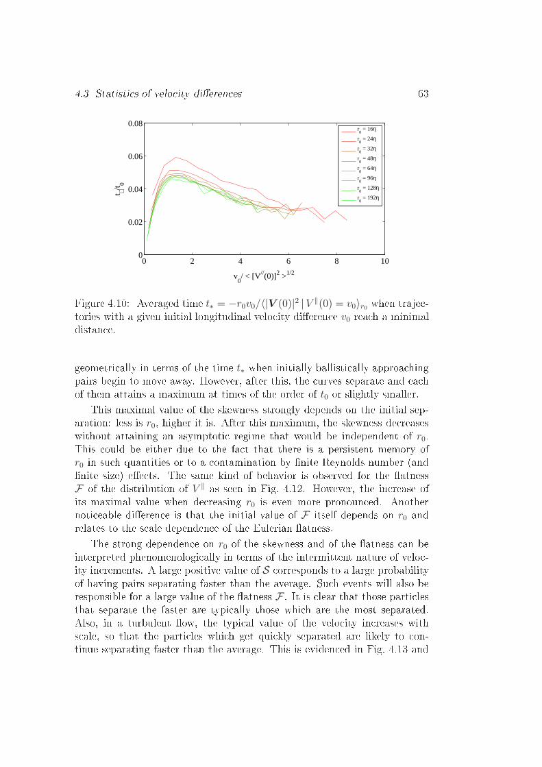
4.3 Statisti s of velo ity dieren es 63

0 2 4 6 8 100

0.02

0.04

0.06

0.08t ∗/t 0

v0/ < [V//(0)]2 >1/2

r0 = 16η

r0 = 24η

r0 = 32η

r0 = 48η

r0 = 64η

r0 = 96η

r0 = 128η

r0 = 192η

Figure 4.10: Averaged time t∗ = −r0v0/〈|V (0)|2 | V ‖(0) = v0〉r0 when traje -tories with a given initial longitudinal velo ity dieren e v0 rea h a minimaldistan e.geometri ally in terms of the time t∗ when initially ballisti ally approa hingpairs begin to move away. However, after this, the urves separate and ea hof them attains a maximum at times of the order of t0 or slightly smaller.This maximal value of the skewness strongly depends on the initial sep-aration: less is r0, higher it is. After this maximum, the skewness de reaseswithout attaining an asymptoti regime that would be independent of r0.This ould be either due to the fa t that there is a persistent memory ofr0 in su h quantities or to a ontamination by nite Reynolds number (andnite size) ee ts. The same kind of behavior is observed for the atnessF of the distribution of V ‖ as seen in Fig. 4.12. However, the in rease ofits maximal value when de reasing r0 is even more pronoun ed. Anothernoti eable dieren e is that the initial value of F itself depends on r0 andrelates to the s ale dependen e of the Eulerian atness.The strong dependen e on r0 of the skewness and of the atness an beinterpreted phenomenologi ally in terms of the intermittent nature of velo -ity in rements. A large positive value of S orresponds to a large probabilityof having pairs separating faster than the average. Su h events will also beresponsible for a large value of the atness F . It is lear that those parti lesthat separate the faster are typi ally those whi h are the most separated.Also, in a turbulent ow, the typi al value of the velo ity in reases withs ale, so that the parti les whi h get qui kly separated are likely to on-tinue separating faster than the average. This is eviden ed in Fig. 4.13 and

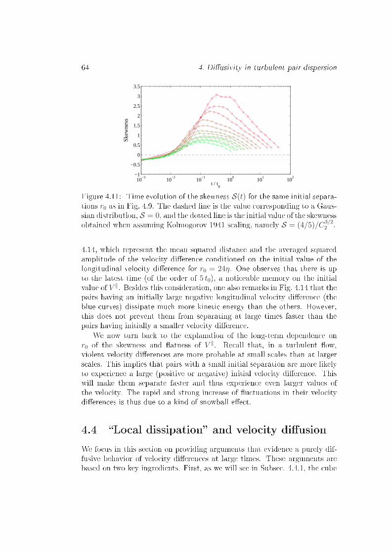
64 4. Diusivity in turbulent pair dispersion

10−3

10−2

10−1

100

101

102

−1

−0.5

0

0.5

1

1.5

2

2.5

3

3.5

Ske

wne

ss

t / t0Figure 4.11: Time evolution of the skewness S(t) for the same initial separa-tions r0 as in Fig. 4.9. The dashed line is the value orresponding to a Gaus-sian distribution, S = 0, and the dotted line is the initial value of the skewnessobtained when assuming Kolmogorov 1941 s aling, namely S = (4/5)/C

3/22 .4.14, whi h represent the mean squared distan e and the averaged squaredamplitude of the velo ity dieren e onditioned on the initial value of thelongitudinal velo ity dieren e for r0 = 24η. One observes that there is upto the latest time (of the order of 5 t0), a noti eable memory on the initialvalue of V ‖. Besides this onsideration, one also remarks in Fig. 4.14 that thepairs having an initially large negative longitudinal velo ity dieren e (theblue urves) dissipate mu h more kineti energy than the others. However,this does not prevent them from separating at large times faster than thepairs having initially a smaller velo ity dieren e.We now turn ba k to the explanation of the long-term dependen e on

r0 of the skewness and atness of V ‖. Re all that, in a turbulent ow,violent velo ity dieren es are more probable at small s ales than at largers ales. This implies that pairs with a small initial separation are more likelyto experien e a large (positive or negative) initial velo ity dieren e. Thiswill make them separate faster and thus experien e even larger values ofthe velo ity. The rapid and strong in rease of u tuations in their velo itydieren es is thus due to a kind of snowball ee t.4.4 Lo al dissipation and velo ity diusionWe fo us in this se tion on providing arguments that eviden e a purely dif-fusive behavior of velo ity dieren es at large times. These arguments arebased on two key ingredients. First, as we will see in Subse . 4.4.1, the ube

4.4 Lo al dissipation and velo ity diusion 65

10−3

10−2

10−1

100

101

102

100

101

102

t / t0

Fla

tnes

s

Figure 4.12: Time evolution of the atness F(t) dened in Eq. (4.30) forthe same initial separations r0 as in Fig. 4.9. The dashed line is the value orresponding to a Gaussian distribution, namely F = 3.velo ity dieren e res aled by the distan e between tra ers, whi h denesa lo al energy dissipation along tra er pairs, attains on short times ales astatisti ally stationary regime. Se ond, as des ribed in Subse . 4.4.2, a eler-ation dieren es between tra ers get un orrelated over very-short times anddata show that their varian e an be related to the aforementioned lo alenergy dissipation. Finally, these onsiderations an be used to apply the entral-limit theorem in order to write down in Subse . 4.4.3 a sto hasti model for the joint time evolution of separations and velo ity dieren es.4.4.1 Stationarity of res aled velo ity dieren esWe have seen in the previous se tions that the velo ity dieren e betweentwo tra ers plays a ru ial role in understanding the me hanisms leading toRi hardson's superdiusive regime for separations. However, the onvergen eof 〈|V (t)|2〉r0 to a behavior ∝ t is not that evident in numeri al data. In ad-dition, as we will see in the next hapter, the statisti s of V (t) display veryintermittent features and, as a onsequen e, does not onverge to a behav-ior with temporal self-similarity, or does it only very slowly. The situationis very dierent when interested in mixed statisti s between distan es andlongitudinal velo ity dieren es. As reported in [Bitane et al., 2012b, themoment 〈[V ‖(t)]3/|R(t)|〉r0, whi h is initially negative and equal to −(4/5)ǫ,tends very qui kly to a positive onstant (see Fig. 4.15).The de rease at very large times omes from the ontamination of thestatisti s by pairs that have rea hed a distan e of the order of the integrals ale. The asymptoti value ≈ 6.2 ǫ seems to depend only weakly on the

66 4. Diusivity in turbulent pair dispersion

10−3

10−2

10−1

100

101

10−1

100

101

102

103

104

t / t0

< |R

(t)|2 |

V// (0

) >

/ r 02

Figure 4.13: Time evolution for r0 = 24η of the averaged distan e ondi-tioned on V ‖(0) = v0 with |v0|/〈[V ‖(0)]2〉1/2r0 = 0.1, 0.4, 0.8, 1.2, ..., 2.8. Thered urves orrespond to positive values of v0 and the blue ones to negativevalues.Reynolds number. The ollapse of the urves asso iated to dierent Reynoldsnumbers and, for r0 ≫ η, to various initial separations indi ate that the timeof onvergen e is ∝ t0. Figure 4.16 shows the same moment but onditionedon the sign of the initial longitudinal velo ity dieren e. One observes thatfor initially separating pairs (red urve), the onvergen e to the asymptoti value is on a time of the order of τη. Conversely for tra ers that initiallyapproa h ea h other (blue urve), the onvergen e is less fast. We have seenin Se . 4.3.2 that su h pairs rst attain their minimal distan e at t ≈ t∗ ≈0.01 t0. Then, at that time, 〈[V ‖(t)]3/|R(t)| | V ‖(0) < 0〉r0 hanges sign andthe onvergen e to ≈ 6.2ǫ o urs only later. Su h initially approa hing pairsare leading the average so that the overall onvergen e is on times ales ofthe order of t∗. The mixed moment 〈[V ‖]3/|R|〉r0, whi h is a kind of lo aldissipation along pairs of traje tories, is thus onserved by the Lagrangianow.A tually, it is not only the average of the lo al dissipation that on-verges to a onstant but its full distribution seems to attain a stationaryregime on times of the order of t∗. Figure 4.17 (a) shows for a given initialseparation, the onvergen e at large times of the PDF of [V ‖(t)]3/|R(t)|. Oneobserves that the right and left tails onverge on dierent times ales. Thetail asso iated to large positive values (separating pairs) o urs on times alesof the order of τη (whi h is in this ase ≈ 0.07 t0), while that for negativevalues (approa hing pairs) onverges slower. For the largest time (t ≈ 5 t0)one observes that deviations to the asymptoti distribution o ur again at

4.4 Lo al dissipation and velo ity diusion 67

10−3

10−2

10−1

100

101

100

101

t / t0

< |V

(t)|2 |

V// (0

) >

/ S 2(r

0)

τηFigure 4.14: Time evolution for r0 = 24η of the averaged squaredvelo ity dieren e onditioned on V ‖(0) = v0 with |v0|/〈[V ‖(0)]2〉1/2r0 =

0.1, 0.4, 0.8, 1.2, ..., 2.8. The red urves orrespond to positive values of v0and the blue ones to negative values. The dashed-dotted line is ∝ t.very large positive values. This is due to a ontamination of su h events bythe large s ales of the turbulent ow. This de rease is in agreement with theobserved departure in Figs. 4.15 and 4.16 of the average from its asymptoti value at large times. Figure 4.17 (b) shows the PDFs of [V ‖]3/|R| for dif-ferent initial separations and at a xed time su iently large to be ensuredthat all distributions have attained their asymptoti regime. One observesa robust ollapse, mu h more pronoun ed than for both the distribution ofseparations and that of velo ity dieren es. Note that in Fig. 4.17 the dis-tributions are raw and were not res aled by any moment of [V ‖]3/|R|. Theasymptoti PDF is peaked around zero (rather than its mean value) anddisplays fat tails that, a ording to our data, are ∝ exp(−C |V ‖|/|R|1/3) onboth sides.To our knowledge, su h a fast and manifest onvergen e of these mixedstatisti s has never been reported before. From a phenomenologi al view-point, one expe ts [V ‖]2 ∝ t ∝ |R|1/3 in the explosive Ri hardsonObukhovregime, so that the lo al dissipation [V ‖]3/|R| should be ome onstant atsu iently large times. However we have observed here that the onvergen eof this quantity to its asymptoti value o urs mu h faster and in a mu hmore denite manner than the onvergen e of the statisti s of |R| and |V |to their respe tive asymptoti forms. This indi ates that the statisti al sta-tionarity of the lo al dissipation is more likely to be a ause rather than a onsequen e of Ri hardsonObukhov explosive separation. At the momentwe unfortunately la k a lear understanding of the physi al me hanisms that

68 4. Diusivity in turbulent pair dispersion

10−2

10−1

100

101

10−1

100

101

t / t0

< [V

// (t)]

3 / |R

(t)|

> /

ε

r0 = 8η

r0 = 12η

r0 = 16η

r0 = 24η

r0 = 32η

r0 = 48η

r0 = 64η

r0 = 96η

Figure 4.15: Time evolution of the mixed moment 〈[V ‖(t)]3/|R(t)|〉r0 fordierent initial separations and the two values of the Reynolds number: Rλ =730 () and Rλ = 460 (+). The bla k dashed line shows the asymptoti value〈[V ‖(t)]3/|R(t)|〉r0 ≈ 6.2 ǫ.are responsible for the observed behavior of [V ‖]3/|R| and that ould shedlight on its relation to explosive separation. We however present in nextse tion its relationship to the statisti s of a eleration dieren es betweentra ers.4.4.2 Statisti s of a eleration dieren esWe ontinue here our study of the times ales entering the relative dispersionpro ess. As already stated in Subse . 4.1.1, the velo ity dieren e V betweenthe two tra ers stays orrelated over a time of the order of the turnovertime τr asso iated to the distan e r between them. This time in reases toofast when the separation |R(t)| in reases. This result makes Ri hardson'sdiusive approa h hardly justiable. However, it is known in turbulent owsthat the a eleration, whi h is a small-s ale quantity, is onversely orrelatedover times that are of the order of the Kolmogorov turnover time τη [Mordantet al., 2004. Its amplitude is rather orrelated on times of the order of thefor ing orrelation time, but this does not alter what argued so far.

4.4 Lo al dissipation and velo ity diusion 69

10−3

10−2

10−1

100

101

−6

−4

−2

0

2

4

6

8

t/t0

< [V

// (t)]

3 / |R

(t)|

> /

ε

τη

−4/5

6.2

(b)

V//(0)>0

V//(0)<0not conditionedFigure 4.16: Time evolution of the mixed moment 〈[V ‖(t)]3/|R(t)|〉r0 for r0 =

24 η and Rλ = 730 (bla k urve) and for the same moment but onditioned onpositive (red urve) and negative (blue urve) values of the initial longitudinalvelo ity dieren e V ‖(0).We have measured the a eleration dieren eA(t) = (∂tu + u · ∇u)(X1(t), t)− (∂tu+ u · ∇u)(X2(t), t) (4.31)between two tra ers. Its Lagrangian auto orrelation fun tion is representedin Fig. 4.18. We learly see that this quantity get un orrelated on timesof the order of τη. This suggests that for separations in the inertial rangeand on times ales mu h longer than the Kolmogorov eddy turnover time,the dieren e of a eleration between two tra ers an be approximated by adelta- orrelated-in-time random pro ess, so that

A ≃√

τ locη A(R,V )η(t), (4.32)where η(t) is the three-dimensional standard white noise. The matrix A isdened asA

TA = 〈A(t)⊗A(t) |R,V 〉r0 . (4.33)Here we have made use of the entral-limit theorem to write Eq. (4.32). Thisimplies that the produ t is there understood in the Stratonovi h sense.Dimensional arguments indi ate that, as they are small-s ale quantities,the lo al Kolmogorov time τ locη and the a eleration amplitude A = |A|depend only on the vis osity ν and on the lo al energy dissipation rate εloc.

70 4. Diusivity in turbulent pair dispersion

−250 −200 −150 −100 −50 0 50 100 150 200 25010

−6

10−5

10−4

10−3

10−2

10−1

[V //]3/[ε|R|]

PD

F

(a) r

0 = 12 ηt = 0

t = 0.02 t0

t = 0.04 t0

t = 0.08 t0

t = 0.17 t0

t = 0.34 t0

t = 0.67 t0

t = 1.3 t0

t = 2.6 t0

t = 5 t0

t = 10 t0

−250 −200 −150 −100 −50 0 50 100 150 200 25010

−6

10−5

10−4

10−3

10−2

10−1

[V //]3/[ε|R|]

PD

F

(b) t ∼ 20 τη

r0 = 4 η

r0 = 6 η

r0 = 8 η

r0 = 12 η

r0 = 16 η

r0 = 24 η

r0 = 32 η

r0 = 48 η

r0 = 64 η

r0 = 96 η

Figure 4.17: (a) PDF of the lo al dissipation [V ‖(t)]3/|R(t)| for r0 = 24 ηand various times (as labeled). (b) Same for various initial separations anda time t = 20 τη xed. t/t0 goes here from 0.2 to 5 so that, in all ases, themixed quantity [V ‖]3/|R| has rea hed its asymptoti regime. In both guresthe verti al dashed lines show the position of the average value ≈ 6.2ǫ.This rate is not only related to energy dissipation but also to energy in-je tion from the larger stru tures of the ow. Approa hes in terms of εlocare frequently used sin e the seminal work of Kolmogorov on rened self-similarity [Kolmogorov, 1962. It was useful to build multifra tal modelsbased on energy dissipation (see, e.g., [Fris h, 1996 and referen es therein)or served for instan e in the study of the statisti s of a eleration ondi-tioned on the velo ity [Biferale et al., 2004. With su h an approa h, the

4.4 Lo al dissipation and velo ity diusion 71

10−1

100

101

102

−0.2

0

0.2

0.4

0.6

0.8

1

t/τ η

〈Ai(

t)A

i(0)〉

r0/〈|

A(0

)|2〉 r

0

r0 = 8ηr0 = 12ηr0 = 16ηr0 = 24ηr0 = 32ηr0 = 48ηr0 = 64ηr0 = 96ηr0 = 96ηr0 = 192η

Figure 4.18: Lagrangian time auto orrelation of the a eleration dieren e〈Ai(t)Ai(0)〉r0 for various r0 and Rλ = 730.lo al Kolmogorov time and the a eleration amplitude an be written as

τ locη ∼ ν1/2 ε−1/2loc and A ∼ ν−1/4 ε

3/4loc . (4.34)This leads to write the diusion oe ient in Eq. (4.32) as

[ τ locη ]1/2A ∼ ε1/2loc . (4.35)It is interesting to note that this quantity is independent on ν and is thusexpe ted to have a nite limit at innite Reynolds numbers. The lo al dissi-pation is a fun tion of the urrent values of the velo ity dieren e V and ofthe separation R. Dimensional arguments suggest that εloc ∼ V 3/R. How-ever, when V = 0, the lo al dissipation is not expe ted to vanish and should ome from an averaged ontribution of larger eddies, leading to εloc ≃ ε, themean dissipation rate. In summary, we expe t to have

εloc(t) ∼ ε+ α[V ‖(t)]3

|R(t)| , (4.36)where α is an adjustable parameter. We have again used here the longitudinalvelo ity dieren e between two tra ers V ‖ = R · V /|R|.All these estimations have been tested against numeri al simulations. Fig-ure 4.19 shows the varian e of the a eleration dieren es onditioned on thelongitudinal velo ity dieren e for various values of the initial separation r0.

72 4. Diusivity in turbulent pair dispersion

−15 −10 −5 0 5 10 150

1

2

3

4

5

6

7

[V ‖]3/(εr0)

〈|A|2|V

‖〉 r

0/[ν

−1/2ε3/2]

r0 = 8ηr0 = 12ηr0 = 16ηr0 = 24ηr0 = 32ηr0 = 48ηr0 = 64ηr0 = 96ηr0 = 96ηr0 = 192ηFigure 4.19: Varian e of the a eleration dieren e amplitude onditionedon the initial longitudinal velo ity dieren e V ‖(0) as a fun tion of the lo aldissipation rate [V ‖(0)]3/r0. The various symbols orrespond to dierentvalues of the separation r0, as labeled.Up to some statisti al errors, it seems that data are in rather good agreementwith the phenomenologi al predi tion given by Eqs. (4.34) and (4.36), whi his represented by the dashed line for α = 0.18.We have here used phenomenologi al onsiderations to express the typi alamplitude of the a eleration dieren e as a fun tion of the distan e betweenpairs and of the velo ity dieren e. These phenomenologi al onsiderationsare purely s alar. They give a good estimate for the varian e of the a elera-tion dieren e modulus but dot not at h the full stru ture of the ovarian etensor. Expressing it more pre isely would require developing further su hphenomenologi al arguments to a ount in parti ular for the in ompressibil-ity of the dynami s. As we will see in next subse tion, we have fo used for themoment on a one-dimensional version of the dynami s where su h tensorial onsiderations are irrelevant. Extending this approa h to higher dimensionsgoes beyond the studies reported in this thesis and is kept for future work.4.4.3 A one-dimensional sto hasti modelWe have seen in previous subse tion that the a eleration dieren e betweentwo tra ers gets un orrelated on a very small times ale. Moreover, its vari-an e an be related to the values of the distan e and of the longitudinalvelo ity dieren e between the two tra ers by dimensional arguments. In

4.4 Lo al dissipation and velo ity diusion 73prin iple, we an then apply the entral-limit theorem to design a model forthe joint time evolution of the separation and of the velo ity dieren e. How-ever, we found an expression for the amplitude of the a eleration, but not forits full tensorial stru ture. We thus fo us here on writing a one-dimensionalmodel that is expe ted to reprodu e the most important features of turbulentpair dispersion.We work here in non-dimensional units. Let us introdu e the followingsto hasti model for the joint evolution of the separation R(t) and the (lon-gitudinal) velo ity dieren e V (t)

dR = V dt, dV = −b|V |R

V dt+

[

1 + c|V |3R

]1/2

dWt, (4.37)where W (t) denotes the one-dimensional Wiener pro ess (see Chap. 3). Themultipli ation by the noise is here understood in the Ito sense. This for-mulation an be seen as an appli ation of the entral-limit theorem to thetime integral of the a eleration dieren e, whi h an be written as a sum ofindependent integrals over time intervals of length τη. The drift term is dueto the hange from Stratonovi h's to Ito's denition of the sto hasti inte-gral. However, the onstants b and c are not dire tly related as their ratiois supposed to ome from tensorial onsiderations and from the pres riptionof in ompressibility to the Lagrangian dynami s. This drift term, whi h isnon-linear, introdu es a orrelation time equal to the turnover time R/|V |.Despite its dependen e on V , this times ale an be seen as a response timeof the pair dynami s whi h depends on both the s ale and the strength ofthe stru ture under onsideration.While its form is relatively simple, the model dened by Eq. (4.37) annotbe integrated expli itly, neither under its sto hasti form, nor with the helpof its equivalent FokkerPlan k form. This is mainly due to the presen e ofnon-linear terms in both the drift and the diusion oe ient. However, we an make the following remarks. Let us write the FokkerPlan k equationfor the transition probability density p(r, v, t|r0, v0, 0) to be separated by rwith a velo ity dieren e v at time t onditioned on the initial onditions,namely∂tp+ v∂rp− ∂v

[

b|v| vr

p

]

= ∂2v

[(

1 + c|v|3r

)

p

]

. (4.38)One an then easily he k that Eq. (4.38) admits s aling solutions of theform p(r, v, t) = tαΨ(r/t3/2, v/t1/2). This s aling exa tly orresponds to thatgiven by Ri hardson's explosive behavior (namely r ∼ t3/2 and v ∼ t1/2).

74 4. Diusivity in turbulent pair dispersionThe fun tion Ψ is a solution of(α+2)Ψ+ ∂ξ

[(

µ− 3

2ξ

)

Ψ

]

= ∂µ

[(

b|µ|µξ

+1

2µ

)

Ψ+ ∂µ

[(

1 + c|µ|3ξ

)

Ψ

]]

.The hoi e α = −2 allows one to get ride of the term ∝ Ψ. This equationthen redu es to a stationary FokkerPlan k equation. However the tradi-tional te hniques used to solve su h problems, as for instan e the assump-tion of onstant probability ux, do not work in that ase and one annotstraightforwardly write a s aling solution for the transition probability den-sity.The di ulties en ountered in solving the FokkerPlan k equation asso- iated to the sto hasti model of Eq. (4.37) led us to investigate its solutionsand statisti al properties by MonteCarlo numeri al simulations. We reportin the rest of this subse tion the results of su h an approa h. Let us rstgive some additional informations on the numeri al settings. First, as thedynami s be omes sti when R → 0, we had to pres ribe a uto at smalldistan es. For that, a minimal s ale η has been introdu ed and, below η,parti les are evolved with a linear velo ity dieren e that is hosen su h thatthey separate in average (this is done in order to mimi a positive Lyapunovexponent at dissipative s ales). The inverse of the rate at whi h the parti lesare separated denes a times ale τη. All results are reported in units of ηand τη. Also, we have not spanned the full parameter spa e by varying sys-temati ally b and c. On the ontrary, we have just fo used on some spe i values and most of the results reported here are for b = 0.1 and c = 0.1.Figure 4.20 (Top) shows the evolution of the mean-squared displa ement〈[R(t)−R(0)]2〉 as a fun tion of time. One learly observes for the model thetwo regimes that are proper to turbulent pair dispersion, namely a ballisti regime ∝ t2 at small times that is followed by an explosive growth of theseparation where 〈R2(t)〉 ∝ t3. With our hoi e of units, ε = 1 and the onstant of proportionality is of the order of 0.1 for c = b = 0.1. One alsonoti es that this large time asymptoti regime is independent of the initialseparation R(0). This indi ates an explosive regime, as in the ase of a tualturbulent pair dispersion. Also, the extension of the ballisti regime learlydepends on R(0). Figure 4.20 (Bottom) shows the time evolution of themean-squared velo ity dieren e. The data reveal a lear diusive behaviorat large times where 〈V 2(t)〉 ∝ t. This law is pre eded by a short in rease ofthe pair kineti energy and of a de rease. While the rst is absent from thedata orresponding to turbulent ow, the se ond has been observed there.To understand better the reasons why the velo ity dieren e be omesdiusive at large times, we have also measured the time evolution of the av-eraged lo al dissipation 〈V 3(t)/R(t)〉. The results are shown in Fig. 4.21.

4.4 Lo al dissipation and velo ity diusion 75

100

101

102

103

100

102

104

106

108

1010

t / τη

< [

R(t

) −

R(0

)]2 >

100

101

102

103

101

102

103

t / τη

< V

2 (t)

>

Figure 4.20: Top: time evolution of the average squared displa ement for thesto hasti model, Eq. (4.37), with c = b = 0.1 for pairs su h that R(0) = 100η(bla k) and R(0) = 1000η (red). The two blue lines stand for the ballisti ∝ t2 regime (on the left) and the explosive ∝ t3 law (on the right). Bottom:Time evolution of the mean squared velo ity dieren e for the same settings.The blue line is the diusive behavior ∝ t.Contrarily to what was observed in real turbulent ows (see Subse . 4.4.1),there is no rapid variation of this quantity on very short times ales. Sur-prisingly, this quantity, whi h is zero at small times by onstru tion in the

76 4. Diusivity in turbulent pair dispersion

100

101

102

103

−8

−6

−4

−2

0

2

t / τη

< V

3 / R

>

Figure 4.21: Time evolution of the mean lo al dissipation 〈V 3(t)/R(t)〉along the solutions to the sto hasti model with c = b = 0.1 and for pairssu h that R(0) = 100η (bla k) and R(0) = 1000η (red).sto hasti ase, be omes relatively qui kly negative. This is related to thede rease of 〈V 2(t)〉 observed in Fig. 4.20 (Bottom). At larger times, this de- rease is then followed by an in rease. Later, similarly to what was observedin real ows, the average lo al dissipation stabilizes to a nite value. Inthe sto hasti model for c = b = 0.1, this limit is of the order of 1. Asseen in Fig. 4.21 this limit seems independent of the initial separation R(0).However, onversely to what observed in real turbulent ows, the times aleof onvergen e to this limit depends on R(0).To omplete our understanding of the behavior of the lo al dissipationalong pair traje tories, we show in Fig. 4.22 their probability density fun -tions estimated at various times. As seen in Subse . 4.4.1 in the ase ofdeveloped turbulent ow, the various urves ollapse together at large timesto an asymptoti distribution with fat tails. In ontrast to the real-ow ase,the left tails seem here less developed than the right ones. The fa t thatthe averaged lo al dissipation 〈V 3(t)/R(t)〉 tends to a positive onstant israther due to a shift of the maximum of the distribution than to a dier-en e in the tails. Note however that the observed u tuations of V 3/R areanyway mu h larger than the measured average value. Events asso iated tolarge value of the lo al dissipation are more frequent for approa hing pairs(V < 0) than for those that separate. This an be due to the fa t that thedynami s asso iated to the model is ompressible. However, by hangingappropriately the values of the parameters b and c, one an ertainly ndvalues where this tenden y is inverted. Anyway, the important suggestion

4.4 Lo al dissipation and velo ity diusion 77

−300 −200 −100 0 100 200 30010

−8

10−6

10−4

10−2

100

V3 / R

PD

F

t = 1.5 τ

η

t = 3.4 τη

t = 7.6 τη

t = 17 τη

t = 38 τη

t = 86 τη

t = 194 τη

t = 437 τη

Figure 4.22: Probability density fun tions of the lo al dissipationV 3(t)/R(t) along the solutions to the sto hasti model with c = b = 0.1and for pairs su h that R(0) = 100η. The various olors orrespond to dif-ferent times, as labeled. Note that the data are not res aled here.made by these measurements is the apparent onvergen e at large times toa s aling regime of the distribution of separations and velo ity dieren es.This onvergen e of the lo al dissipation, together with the long-timebehaviors observed earlier in this subse tion for the squared average quanti-ties, are very similar to those obtained for tra er relative dispersion in turbu-lent ows. Also, they give eviden e that the s aling regime dis ussed abovein the framework of the FokkerPlan k equation ould be attained by themodel at large times. This asymptoti behavior is eviden ed by looking atthe probability distributions of the displa ement and the velo ity dieren esthemselves. As seen in Fig. 4.23, on e res aled by their standard deviations,both of them onverge at large times to asymptoti distributions, onrmingwhat expe ted. The velo ity probability density fun tion, whi h was hosenGaussian at the initial time, qui kly develops fat tails. This is ertainly dueto the non-linear nature of the multipli ative noise in the sto hasti model.The separation distribution is also developing a fat tail at large values. Asseen in Fig. 4.23 (Top), these tails be ome more stret hed than an expo-nential in the large-time asymptoti s aling distribution. However, we werenot able to mat h them with Ri hardson's diusive distribution dis ussed inSubse . 4.1.1.

78 4. Diusivity in turbulent pair dispersion

0 2 4 6 8 10

10−4

10−3

10−2

10−1

100

101

R / <R2(t)>

PD

F

−10 −5 0 5 1010

−6

10−5

10−4

10−3

10−2

10−1

100

V / <V2>1/2

PD

F

Figure 4.23: Top: probability density fun tion of the separation R betweentwo traje tories obtained from the sto hasti model with b = c = 0.1 andR(0) = 100. The dierent olors orrespond to the dierent times shown inFig. 4.22. Bottom: same for the velo ity dieren e V .

The probability distribution of the separation is also developing tails atsmall values. This is lear in Fig. 4.24 where they are represented not res aledand in log-log oordinates. One observes there that the probability densityfun tion of the separation p(R) develops at small values a power-law behaviorp(R) ∝ Rα where the exponent α depends on time. Initially it is equal to+∞ as the distribution is entered on R = R(0) and it onverges to anasymptoti value ≈ −0.5 at large times. This value depends on the hoi e

4.4 Lo al dissipation and velo ity diusion 79

100

101

102

103

104

105

10−8

10−6

10−4

10−2

R / η

PD

F

Figure 4.24: Probability density fun tion of the separation R between twotraje tories obtained from the sto hasti model with R(0) = 100η. Thedierent olors orrespond to the same times as in Fig. 4.22. Note that thistime the distributions are not res ales and are shown in log-log oordinatesto eviden e the behavior at small separations.of the parameters b and c. The fa t that it is negative is a lear signatureof the ompressibility of the one-dimensional sto hasti model studied here.However, the intermediate time variations of α are mu h more relevant. Also,as seen in Fig. 4.24, one observes that at intermediate times, the exponent αis smaller than its asymptoti value, so that its behavior is non-monotoni .At su h intermediate times, the pair distribution is thus more on entrated atsmall distan es than at later times. This behavior is indi ating the presen e ofstrong u tuations in the statisti s of pair dispersion. Su h extreme eventsare important as they relate to the probability of a slow dispersion of thetransported spe ies. As we will see in the next hapter, this behavior analso be observed for relative dispersion in a tual developed turbulent ows.To on lude, let us stress again that, so far, we have only investigated asimple one-dimensional version of the proposed model Eq. (4.37). We believethat extensions to higher dimensions will make this kind of approa h morerelevant to a tual turbulent pair dispersion. However, the main issue willthen be to a ount for in ompressibility via the tensorial stru ture of thea eleration varian e. This goes beyond the aim of the present study and itwill be investigated in a future work.

80 4. Diusivity in turbulent pair dispersion

Chapter 5Geometry and violent events inturbulent relative motionHere we arry on our study of the statisti s of Lagrangian pair dispersionin a homogeneous isotropi ow. Again, we mostly use the results of high-resolution dire t numeri al simulations. In previous hapter, we have seenthat the squared average quantities are well des ribed by Ri hardson's eddy-diusivity approa h. An example is the t3 behavior for the mean-squareddistan e between tra ers, whi h seems rather robust. We however dis ussedthe fa t that the main assumption in this approa h is hard to justify. Thevelo ity dieren e is indeed orrelated on times that are always longer orof the order of the onsidered times ales. For this reason, we have givena reinterpretation of the t3 in terms of a diusive behavior of the velo itydieren es. This hypothesis has been justied by investigating the orrelationof a eleration dieren es.In this hapter, the fo us is again on the deviations from Ri hardson'seddy-diusivity model. Our attention is on the strong u tuations that areexperien ed by tra ers. For that we rst investigate in Se . 5.1 the high-ordermoments of separation and velo ity dieren es. Eviden e is obtained that thedistribution of distan es attains an almost self-similar regime hara terizedby a very weak intermitten y. The times ale of onvergen e to this behavioris found to be given by the kineti energy dissipation time t0 measured at thes ale of the initial separation and whi h was introdu ed in previous hapter.Conversely the velo ity dieren es between tra ers are displaying a stronglyanomalous behavior whose s aling properties are very lose to that of La-grangian stru ture fun tions. We then give a geometri al interpretation ofthese violent u tuations and show that they are responsible for a long-termmemory of the initial separation.These results are then brought together to address the question of violent81

82 5. Geometry and violent events in turbulent relative motionevents in the distribution of distan es. We report in Se . 5.2 our ndingsthat distan es mu h larger than the average are rea hed by pairs that havealways separated faster sin e the initial time. They are responsible for thepresen e of a stret hed exponential behavior in the tail of the inter-tra erdistan e probability distribution. The tail approa hes a pure exponential atlarge times, ontradi ting Ri hardson's diusive approa h. At the same time,as we show in Se . 5.3, the distan e distribution displays a time-dependentpower-law behavior at very small values, whi h is interpreted in terms offra tal geometry. It is argued and demonstrated numeri ally that the ex-ponent onverges to one at large time, again in oni t with Ri hardson'sdistribution.5.1 High-order statisti s5.1.1 S aling regime in the statisti s of distan esWe have seen in the previous hapter (Se . 4.2) that the mean squared dis-pla ement 〈|R(t) − R(0)|2〉r0 between two tra ers that were initially at adistan e |R(0)| = r0, behaves ballisti ally as t2 for small times and explo-sively as t3 at large times. We re all that R(t) = X2(t) − X1(t) denotesthe separation between two tra ers. We showed that the transition betweenthe two aforementioned regimes o urs at a time t0 = S2(r0)/(2ε), whereS2(r0) is the absolute-value se ond-order Eulerian stru ture fun tion of theuid velo ity over a distan e r0 and ε is the average turbulent rate of kineti energy dissipation. In this se tion, we turn to investigating the large-timebehavior of higher-order moments of the separation. Figures 5.1 (a) and (b)show the time evolution of 〈|R(t) − R(0)|4〉r0 and of 〈|R(t) − R(0)|6〉r0,respe tively. At times smaller than t0 the separation grows ballisti ally,so that 〈|R(t) − R(0)|p〉r0 ≃ tp 〈|V (0)|p〉r0 where we re all that V (t) =u(X2, t) − u(X1, t) denotes the velo ity dieren e between the two tra ers.The fa t that we have hosen to res ale time by t0 (whi h depends on se ond-order statisti s of the initial velo ity dieren e) implies that the moments donot ollapse in this regime be ause of Eulerian multis aling. However the ollapse o urs for t ≫ t0 where these two moments grow like t6 and t9,respe tively, with possible minute deviations. The measured power-laws giveeviden e that, at su iently long times, inter-tra er distan es follow a s ale-invariant law. Also the observed ollapses indi ate that t0 ould be again thetime of onvergen e to su h a behavior.The presen e of a s ale-invariant regime is also lear when making use ofideas borrowed from extended self-similarity and representing these two mo-

5.1 High-order statisti s 83

10−3

10−2

10−1

100

101

102

10−10

10−5

100

105

1010

t / t0

<|R

(t)−

R(0

)|4 > /

(ε2 t 06 )

(a)

10−3

10−2

10−1

100

101

102

10−15

10−10

10−5

100

105

1010

1015

t / t0

<|R

(t)−

R(0

)|6 > /

(ε3 t 09 )

(b)

r0 = 4η

r0 = 6η

r0 = 8η

r0 = 12η

r0 = 16η

r0 = 24η

r0 = 32η

r0 = 48η

r0 = 64η

r0 = 96ηFigure 5.1: (a) Fourth-order moment 〈|R(t)−R(0)|4〉r0 and (b) sixth-ordermoment 〈|R(t) − R(0)|6〉r0 as fun tion of t/t0 for Rλ = 730. Both urvesare normalized su h that their expe ted long-time behavior is ∝ (t/t0)

6 and∝ (t/t0)

9, respe tively. The bla k dashed lines represent su h behaviors.ments as a fun tion of 〈|R(t)−R(0)|2〉r0 (see Fig. 5.2). This time, for a xedr0, the smallest separations orrespond to the ballisti regime. There, we triv-ially have 〈|R(t)−R(0)|p〉r0/〈|R(t)−R(0)|2〉p/2r0 ≃ 〈|V (0)|p〉r0/〈|V (0)|2〉p/2r0 ,whi h has a weak dependen e on r0, be ause of an intermittent distributionof Eulerian velo ity in rements, but does not depend on time. This normals aling an be observed for t ≪ t0 in the insets of Fig. 5.2, whi h representthe logarithmi derivatives of the high-order moments with respe t to these ond order. At times of the order of t0, noti eable deviations to normals aling an be observed. Finally, at mu h larger s ales, data orrespondingto dierent values of the initial separation r0 ollapse but the urves startto bend down. One observes in the insets that the asso iated lo al slopesapproa h values learly smaller than those orresponding to normal s aling.

84 5. Geometry and violent events in turbulent relative motion

10−8

10−6

10−4

10−2

100

10−15

10−10

10−5

100

<|R(t)−R(0)|2> / L2

<|R

(t)−

R(0

)|4 > /

L4

(a)

10−3

10−2

10−1

100

101

102

1.8

2

2.2

t / t0

loca

l slo

pe

10−8

10−6

10−4

10−2

100

10−25

10−20

10−15

10−10

10−5

100

<|R(t)−R(0)|2> / L2

<|R

(t)−

R(0

)|6 > /

L6

(b)

r0 = 4η

r0 = 6η

r0 = 8η

r0 = 12η

r0 = 16η

r0 = 24η

r0 = 32η

r0 = 48η

r0 = 64η

r0 = 96η

10−3

10−2

10−1

100

101

102

2.5

3

3.5

t / t0

loca

l slo

pe

Figure 5.2: Fourth (a) and sixth (b) order moments of |R(t) −R(0)| as afun tion of its se ond-order moment for Rλ = 730. The two gray dashed linesshow a s ale-invariant behavior, i.e. 〈|R(t)−R(0)|4〉r0 ∝ 〈|R(t)−R(0)|2〉2r0and 〈|R(t)−R(0)|6〉r0 ∝ 〈|R(t)−R(0)|2〉3r0, respe tively. The two in-sets show the asso iated lo al slopes, that is the logarithmi derivativesd log〈|R(t)−R(0)|p〉r0/d log〈|R(t)−R(0)|2〉r0 , together with the normal s al-ings represented as dashed lines.This gives eviden e of a rather weak intermitten y in the distribution oftra er separations. Note that the presented measurements were performedfor Rλ = 730 but the same behavior has been observed for Rλ = 460. Werefer the reader to Subse . 4.2.1 for further details on the parameters of thenumeri al simulations.To our knowledge, the most onvin ing observation of an intermittentbehavior in pair dispersion has been based on an exit-time analysis [Boetta& Sokolov, 2002a,Biferale et al., 2005. However, the relation of su h xed-s ale statisti s to the usual xed-time measurements we report here requires

5.1 High-order statisti s 85

0 1 2 3 4

10−8

10−6

10−4

10−2

100

102

[ r / <|R(t)|2>1/2 ]2/3

<|R

(t)|2 >

3/2 p

(r)

/ (4

π r2 )

(a) t = 2.5 t0

r0 = 2 η

r0 = 3 η

r0 = 4 η

r0 = 6 η

r0 = 8 η

r0 = 12 η

r0 = 16 η

r0 = 24 η

0 1 2 3 4

10−8

10−6

10−4

10−2

100

102

[ r / <|R(t)|2>1/2 ]2/3

<|R

(t)|2 >

3/2 p

(r)

/ (4

π r2 )

(b) t = 5 t0

r0 = 2 η

r0 = 3 η

r0 = 4 η

r0 = 6 η

r0 = 8 η

r0 = 12 η

r0 = 16 η

r0 = 24 η

Figure 5.3: Probability density fun tion of the distan e r at time t = 2.5 t0(a) and t = 5 t0 (b) and for various values of the initial separation. We havehere normalized it by 4πr2 and represented on a log y axis as a fun tion ofr/〈|R(t)|2〉1/2r0 . With su h a hoi e, Ri hardson's diusive density distribution(4.9) appears as a straight line (represented here as a bla k dashed line).to onsider pair separation velo ities. As we will see in the next subse tion,the velo ity dieren e between two tra ers displays statisti s that are mu hmore intermittent than those for pair separation. This implies that there isno ontradi tion between an almost normal s aling for distan es as a fun tionof time and an anomalous behavior of exit times as a fun tion of distan e.To investigate further this weak intermitten y in the separation distribu-tion, we have represented in Fig. 5.3 the probability density fun tion (PDF)

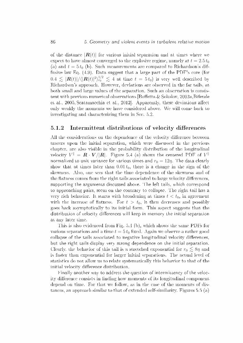
86 5. Geometry and violent events in turbulent relative motionof the distan e |R(t)| for various initial separation and at times where weexpe t to have almost onverged to the explosive regime, namely at t = 2.5 t0(a) and t = 5 t0 (b). Su h measurements are ompared to Ri hardson's dif-fusive law Eq. (4.9). Data suggest that a large part of the PDF's ore (for0.4 . |R(t)|/〈|R(t)|2〉1/2r0 . 4 at time t = 5 t0) is very well des ribed byRi hardson's approa h. However, deviations are observed in the far tails, atboth small and large values of the separation. Su h an observation is onsis-tent with previous numeri al observations [Boetta & Sokolov, 2002a,Biferaleet al., 2005, S atama hia et al., 2012. Apparently, these deviations ae tonly weakly the moments we have onsidered above. We will ome ba k toinvestigating and hara terizing them in Se . 5.2.5.1.2 Intermittent distributions of velo ity dieren esAll the onsiderations on the dependen e of the velo ity dieren e betweentra ers upon the initial separation, whi h were dis ussed in the previous hapter, are also visible in the probability distribution of the longitudinalvelo ity V ‖ = R · V /|R|. Figure 5.4 (a) shows the entered PDF of V ‖normalized to unit varian e for various times and r0 = 12η. The data learlyshow that at times later than 0.01 t0, there is a hange in the sign of theskewness. Also, one sees that the time dependen e of the skewness and ofthe atness omes from the right tails asso iated to large velo ity dieren es,supporting the arguments dis ussed above. The left tails, whi h orrespondto approa hing pairs, seem on the ontrary to ollapse. The right tail has avery ri h behavior. It starts with broadening at times t < t0, in agreementwith the in rease of atness. For t > t0, it then de reases and possiblygoes ba k asymptoti ally to its initial form. This aspe t suggests that thedistribution of velo ity dieren es will keep in memory the initial separationat any later time.This is also eviden ed from Fig. 5.4 (b), whi h shows the same PDFs forvarious separations and a time t = 5 t0 xed. Again we observe a rather good ollapse of the tails asso iated to negative longitudinal velo ity dieren es,but the right tails display very strong dependen e on the initial separation.Clearly, the behavior of this tail is a stret hed exponential for r0 . 8η andis faster than exponential for larger initial separations. The a tual level ofstatisti s do not allow us to relate systemati ally this behavior to that of theinitial velo ity dieren e distribution.Finally another way to address the question of intermitten y of the velo -ity dieren e onsists in nding how moments of its longitudinal omponentdepend on time. For that we follow, as in the ase of the moments of dis-tan es, an approa h similar to that of extended self-similarity. Figures 5.5 (a)

5.1 High-order statisti s 87

−8 −6 −4 −2 0 2 4 6 810

−5

10−4

10−3

10−2

10−1

100

[V //(t) − <V//(t)>] / <[V //(t) − <V//(t)>]2>1/2

PD

F

(a) r

0 = 12η

t = 0t = 0.1 t

0

t = 0.5 t0

t = 0.9 t0

t = 2 t0

t = 4 t0

t = 7 t0

t = 10 t0

Gaussian

−4 −2 0 2 4 610

−5

10−4

10−3

10−2

10−1

100

[V //(t) − <V//(t)>] / <[V //(t) − <V//(t)>]2>1/2

PD

F

(b) t = 5 t

0

r0 = 2η

r0 = 3η

r0 = 4η

r0 = 6η

r0 = 8η

r0 = 12η

r0 = 16η

r0 = 24η

GaussianFigure 5.4: Centered and normalized probability density fun tions of thelongitudinal velo ity dieren e: (a) for r0 = 12 η and various times and (b)for various initial separations and t = 5 t0. In both ases, the bla k dashedline shows a Gaussian distribution.and (b) show the fourth and sixth-order moments of V ‖(t) as a fun tion of itsse ond-order moment. As eviden ed in the insets, they display an anomalousbehavior that diers from simple s aling. However, the ollapse for variousr0 is mu h less evident than for the moments of the distan e, ex ept perhapsat su iently large times. One an there guess a power-law dependen e of〈[V ‖(t)]p〉r0 as a fun tion of 〈[V ‖(t)]2〉r0. Surprisingly the power is ompatiblewith the s aling exponent of the Lagrangian stru ture fun tions that wereobtained in [Biferale et al., 2004 by relating velo ity in rement along tra-

88 5. Geometry and violent events in turbulent relative motion

10−2

10−1

100

10−2

10−1

100

101

102

<V//2(t)> / u

rms2

<V

//4 (t)>

/ u rm

s4

(a)

10−3

10−2

10−1

100

101

102

0

2

4

t / t0

loca

l slo

pe

10−2

10−1

100

10−2

10−1

100

101

102

103

<V//2(t)> / u

rms2

<V

//6 (t)>

/ u rm

s6

(b)

r0 = 16η

r0 = 24η

r0 = 32η

r0 = 48η

r0 = 64η

r0 = 96η

r0 = 128η

r0 = 192η

10−3

10−2

10−1

100

101

102

0

2

4

6

t / t0

loca

l slo

pe

Figure 5.5: Fourth-order (a) and sixth-order (b) moments of the longitudi-nal velo ity dieren e as a fun tion of its se ond-order moment for varioustimes and initial separations. The two dashed lines orrespond to a s aling ompatible with that of Lagrangian stru ture fun tions proposed in [Biferaleet al., 2004, namely ζL4 /ζL2 = 1.71 and ζL6 /ζ

L2 = 2.16. The insets show thelogarithmi derivative d log〈[V ‖(t)]p〉r0/d log〈[V ‖(t)]2〉r0 for (a) p = 4 and (b)

p = 6 as a fun tion of t/t0; there the bold dashed lines show the Lagrangianmultifra tal s aling and the thin lines what is expe ted from a self-similarbehavior.je tories to SheLévêque multifra tal spe trum for the Eulerian eld. Thetwo dashed lines in Fig. 5.5 (a) and (b) orrespond to the predi ted valuesζL4 /ζ

L2 = 1.71 and ζL6 /ζ

L2 = 2.16. Conrming further that this mat h wouldrequire mu h better statisti s.

5.2 Memory in large-distan e statisti s 895.2 Memory in large-distan e statisti sIn this se tion and in the following we turn ba k to the statisti s of the dis-tan e |R(t)| between two tra ers. Our goal is to explain the me hanismsleading to very large or very small values of this distan e in the light of thevarious observations made in previous se tions and in previous hapter. Con-sidering the relative dispersion of tra ers onditioned on their initial distan er0 an be geometri ally interpreted in terms of the time evolution of an ini-tially spheri al surfa e of radius r0 that is entered on a referen e traje tory.The transport of this surfa e by a turbulent ow is generally very omplex.In ompressibility implies that the volume of the sphere is onserved but thevelo ity eld roughness will be responsible for strong distorsions of its sur-fa e. This is represented in Fig. 5.6 that shows for Rλ = 460 at three varioustimes the shape dened by the instantaneous position of 60 traje tories thatare all initially at a distan e 24η from a referen e tra er.

Figure 5.6: Quasi-Lagrangian evolution of the set of tra ers that are initiallyat a distan e r0 = 24η of a referen e traje tory.We an qualitatively dedu e from these snapshots that the large ex ur-sions of the inter-traje tory distan e go together with strong pin hes of thesurfa e. We also see that the intense stret hings are o urring in a time- orrelated manner: the surfa e angles that are visible at late time haveformed at very early stages. As we will now see, the most-separated pairshave been so for long times and arry a reminis ent dependen e on the initialseparation.We rst onsider in this se tion the events related to distan es that aremu h larger than their average. It was argued in Se . 5.1.1 that the large-value tail of the separation PDF is not well des ribed by Ri hardson's dis-tribution. As seen in Fig. 5.3 (b) for t = 5 t0, the tail is indeed broader than

90 5. Geometry and violent events in turbulent relative motionexp(−C |R|2/3) for r0 . 8η and narrower otherwise. It seems to tend to aGaussian when either r0 or t are su iently large. We have he ked thatthese behaviors are not due to a ontamination by pairs that have rea hedthe large s ales of the turbulent ow, as the onsidered distan es are still wellbelow L, ex ept maybe for the largest initial separation r0 = 24η. These ob-servations suggest that for su h extreme events, there is a long-term memoryof the initial separation.To qualify further the history of pairs that are well separated at largetimes, we have performed the following analysis. Fixing a nal time tf suf- iently large to have rea hed the explosive Ri hardsonObukhov regime,we have arried out statisti s onditioned on pairs that are far separated att = tf , say su h that their distan e is |R(tf)| ≥ 2 〈|R(tf)|〉r0. In order tonot be ontaminated by nite inertial subrange ee ts, we have restri tedthis analysis to Rλ = 730 and to initial separations 2 η ≤ r0 ≤ 24 η, andwe have hosen the largest ompatible value of tf , namely tf = 5 t0. Letus denote by 〈·〉+ the resulting onditional ensemble average, i.e. 〈·〉+ =〈· | |R(tf)| ≥ 〈|R(tf)|〉r0〉r0 . Figure 5.7 (a) represents the relative in rease〈|R(t)−R(0)|2〉+/〈|R(t)−R(0)|2〉r0 of the mean-squared displa ement. Thevarious urves, whi h are asso iated to dierent initial separations r0, havea maximum at t = tf = 5 t0 represented by a dashed line. The value of thismaximum is be oming larger when r0 de reases and approa hes the dissipa-tive s ales. This is a signature of the dependen e of the large-positive valuetail upon r0. On the right-hand side of the maximum, the various urves tendba k to 1. This indi ates that separations that are large at a given interme-diate time relax in average to an ordinary behavior at later times. This anbe regarded as a onsequen e of the weakening of large-distan e probabilitytails as a fun tion of time. The situation is rather dierent when interestedin the left-hand side of the maximum. The urves do not onverge to 1, andthus to an average behavior when t → 0. This means that pairs that are wellseparated at a given time are likely to have been so at any previous times.This asymmetry when going forward or ba kward in time ould already begrasped in Fig. 5.6. The traje tories that are far away from the referen etra er at the latest time (as, e.g., those dening the left and top orners)are visibly also well separated at the intermediate time. Conversely the right orner at the intermediate time have later stopped separating faster than theaverage.Figure 5.7 (b) shows the time evolution of the averaged longitudinal velo -ity dieren e 〈V ‖(t)〉+ onditioned on having a separation twi e the averageat time tf = 5 t0. A rst remark that annot be seen from the log-log plot isthat the initial value of this average is stri tly positive. The inset representsthe variation of 〈V ‖(0)〉+ as a fun tion of the initial separation. This implies

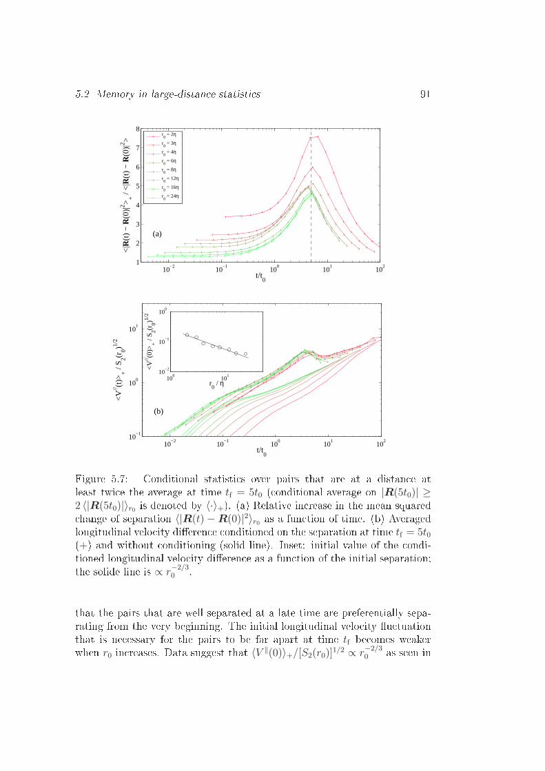
5.2 Memory in large-distan e statisti s 91

10−2

10−1

100

101

102

1

2

3

4

5

6

7

8

t/t0

<|R

(t)

− R

(0)|2 >

+ /

<|R

(t)

− R

(0)|2 >

(a)

r0 = 2η

r0 = 3η

r0 = 4η

r0 = 6η

r0 = 8η

r0 = 12η

r0 = 16η

r0 = 24η

10−2

10−1

100

101

102

10−1

100

101

t/t0

<V

// (t)>

+ /

S 2(r0)1/

2

(b)

100

101

10−2

10−1

100

r0 / η

<V

// (0)>

+ /

S 2(r0)1/

2

Figure 5.7: Conditional statisti s over pairs that are at a distan e atleast twi e the average at time tf = 5t0 ( onditional average on |R(5t0)| ≥2 〈|R(5t0)|〉r0 is denoted by 〈·〉+). (a) Relative in rease in the mean squared hange of separation 〈|R(t)−R(0)|2〉r0 as a fun tion of time. (b) Averagedlongitudinal velo ity dieren e onditioned on the separation at time tf = 5t0(+) and without onditioning (solid line). Inset: initial value of the ondi-tioned longitudinal velo ity dieren e as a fun tion of the initial separation;the solide line is ∝ r

−2/30 .that the pairs that are well separated at a late time are preferentially sepa-rating from the very beginning. The initial longitudinal velo ity u tuationthat is ne essary for the pairs to be far apart at time tf be omes weakerwhen r0 in reases. Data suggest that 〈V ‖(0)〉+/[S2(r0)]

1/2 ∝ r−2/30 as seen in

92 5. Geometry and violent events in turbulent relative motion

10−2

10−1

100

101

102

103

0

0.5

1

1.5

2

t/t0

Exp

onen

t α

Gaussian

Exponential

Richardson

r0 = 2 η

r0 = 3 η

r0 = 4 η

r0 = 6 η

r0 = 8 η

r0 = 12 η

r0 = 16 η

r0 = 24 η

r0 = 32 η

r0 = 48 η

r0 = 64 η

r0 = 96 η

r0 = 128 ηFigure 5.8: Exponent α of the right tail of the PDF of distan es |R(t)|as a fun tion of time and for various initial separations. The exponent wasobtained by tting − log p(|R|) to a power-law for 〈|R(t)|〉r0 < |R(t)| <

0.5L.the inset. This initial separation makes the sele ted pairs rea h an almostdiusive regime at time mu h shorter than the end of the average ballisti regime. For large-enough initial separations we indeed have 〈V ‖(t)〉+ ∼ t1/2for 0.1 t0 . t . t0. The pair distan e en ountered a nal a eleration beforeattaining the onditioning. After that, the longitudinal velo ity dieren erelaxes slowly to the average regime. Again here, as in the ase of the av-erage separation, we observe that the imposing of having a large distan eat a large time sele ts pair histories. The main ontribution to statisti s isindeed given by ouples en ountering an initially violent separation that isthen followed by a rapid onvergen e to an explosive regime.In order to give a more quantitative handle on the far tail of the sepa-ration PDF, we have estimated and tted its fun tional shape and studiedits variations. For that, following the observations made in Se . 5.1.1, wehave assumed that p(|R|) ∝ exp(−C |R|α) and measured how the exponentα depends on both time and initial separation.Figure 5.8 shows the time behavior of the exponent α for various valuesof the initial separation. On the gure, the three dashed horizontal linesrepresent the tails of a Gaussian (α = 2), of an exponential (α = 1) andof Ri hardson's distribution (α = 2/3). At time t = 0, the distribution ispeaked around r0 and ompa tly supported, so that α = ∞. The exponentthen de reases, rosses α = 1 (so that the distribution be omes a stret hed

5.3 Fra tal distribution at small distan es 93exponential) for t ≈ 0.1 t0, and rea hes a minimal value that depends onthe initial separation r0. For the smallest r0, this minimal value is belowRi hardson's predi tion, as previously noti ed. For larger separations, thisminimum in reases and when r0 ≫ η the urves seem to saturate to the valueα = 1. Also, we annot ex lude that all urves onverge to the exponentialvalue when t → ∞. The in rease at the last stage an hardly be blamedon an integral-s ale ee t. We have indeed ex luded here all pairs that areseparated by a distan e larger than L/2.5.3 Fra tal distribution at small distan esMu h more violent and intermittent events take pla e for parti le pairs thatseparate mu h less than the average. As already stressed and observed inFig. 5.6, the large ex ursions of inter-traje tory distan es go together withstrong pin hes of separations.This is eviden ed from Fig. 5.9 that represents the probability distribu-tion of |R| at various times and for two inertial-range values of the initialseparation. One observes that at very short times, the PDF is peaked aroundr0. When time in reases, its maximum, whi h roughly orresponds to thevalue of 〈|R(t)|〉r0, shifts to larger values and the distribution broadens si-multaneously at large and small values. This leads to the development forr0 ≪ |R| ≪ 〈|R|〉r0 of an intermediate range of pairs whose separations lagbehind the average evolution. In this subrange, the PDF behaves as a powerlaw p(|R|) ∝ |R|β, where the exponent β evolves as a fun tion of time andr0. The power-law behavior is substantiated when measuring the umulativeprobability P<(r) = Prob[|R| < r] =

∫ r

0p(r′) dr′ ∝ rβ+1 of inter-traje torydistan es. One expe ts from Ri hardson's arguments that β = 2, so that

P<(r) ∝ r3. The exponent β an be interpreted in terms of fra tal geometry.If all the traje tories were uniformly and independently distributed in spa e,the fra tion of pairs at a distan e less than r would be ∝ rd, where d = 3is the spa e dimension. Also one would expe t this fra tion to be ∝ rd−1 ifthe traje tories were all onned on a surfa e, and ∝ rd−2 if they were on a urve. In general, the exponent β + 1 = limr→0[logP<(r)]/[log r] measuresthe orrelation dimension of a fra tal set. Ri hardson's r2 behavior thus or-responds to the idea that, at su iently long times, traje tories forget abouttheir initial separation and distribute homogeneously in spa e.As we have previously dis ussed, pair dispersion an be geometri ally in-terpreted as the average Lagrangian evolution of an initially spheri al surfa eof radius r0 entered on a referen e traje tory. At time t = 0, it is lear that

P<(r) is a Heaviside fun tion entered on r = r0, so that β = ∞. At later

94 5. Geometry and violent events in turbulent relative motion

100

102

104

10−6

10−4

10−2

100

|R| / η

PD

F

(a) r

0 = 12η

r0

t = 0.059 t0

t = 0.12 t0

t = 0.24 t0

t = 0.47 t0

t = 0.94 t0

t = 1.8 t0

t = 3.6 t0

t = 7.1 t0

100

102

104

10−6

10−4

10−2

100

|R| / η

PD

F

(b) r

0 = 24η

r0

t = 0.029 t0

t = 0.058 t0

t = 0.12 t0

t = 0.23 t0

t = 0.46 t0

t = 0.89 t0

t = 1.8 t0

t = 3.4 t0Figure 5.9: Uns aled PDFs of the absolute separation between tra ers forvarious times and the initial separations (a) r0 = 12 η and (b) r0 = 24 η.times the stret hing and pin hing of the sphere leads to a non-trivial behav-ior of P<(r) for r ≪ 〈|R|〉r0. This behavior is sket hed for two dimensionsin Fig. 5.10. The exponent β is thus measuring the fra tality of the image ofthe sphere by the Lagrangian ow. It relates to the fra tion of this forward-in-time image that remains within a distan e r of the referen e traje tory. Atsu iently large times (right-most panel of Fig. 5.10), one expe ts the set of

5.3 Fra tal distribution at small distan es 951

r

r0

t = t > 0t = 0

r

t >> t1

Figure 5.10: Two dimensional sket h of the time evolution of traje toriesthat are initially lo ated at a distan e r0 of a referen e tra er (shown as abla k dot at the enter of the ir le) and then spread.traje tories to be mainly stret hed by the ow eddies with the most relevant orrelation time, that is those of size 〈|R(t)|〉r0, and the small s ale u tua-tions to be ome less and less important. Hen e, at s ales r ≪ 〈|R(t)|〉r0 andvery large times, the only remaining pairs should be distributed on a surfa e( urve in two dimensions), so that β + 1 ≃ 2 and p(r) ∝ r. This approa h ontradi ts the predi tion of Ri hardson that, somehow, postulates that thevelo ity dieren e orrelation time does not depend on s ale (as it is assumedto be zero).To shed light on su h ideas, we have estimated the exponent β for variousr0 and at dierent times. For this purpose, we have used the umulativeprobability P<(r) (shown in Fig. 5.11 (a) for r0 = 4η) to obtain β + 1through a t of its lo al slope. The resulting measurements are displayedin Fig. 5.11 (b) as a fun tion of time. Up to the largest error bars due toa la k of statisti s, one observes that the times ale t0 is again relevant todes ribe both the initial dynami s and the onvergen e to an asymptoti regime. At small times t ≪ t0, the exponent β takes large positive values,whi h, as explained above, are due to the initial onditioning |R(t)| = r0.At time t ≈ 0.3 t0, the exponent be omes smaller than 3. For t ≫ t0, itasymptoti ally approa hes the value β = 2, so that data give eviden e in favorof the argument exposed above. Interestingly, for small initial separationsr0 . 16η, the limit is rea hed from below and pre eded by a minimum of β.This means that for su h intermediate times, the pin hing (or equivalentlythe stret hing) of the sphere is so strong that the interse tion of the latterwith spheres of radius r denes a fra tal obje t that is more on entratedthan a surfa e. Su h a temporary singular behavior is ertainly related tothe presen e of tails fatter than exponential at very large distan es.

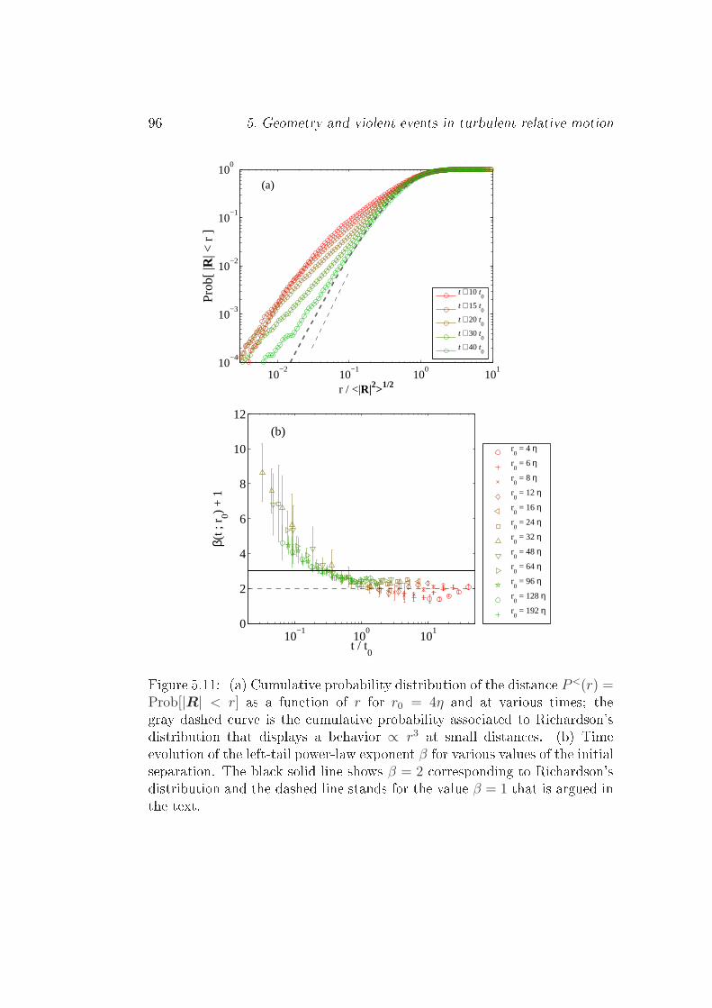
96 5. Geometry and violent events in turbulent relative motion

10−2

10−1

100

101

10−4

10−3

10−2

10−1

100

r / <|R|2>1/2

Pro

b[ |R

| < r

]

(a)

t ∼ 10 t0

t ∼ 15 t0

t ∼ 20 t0

t ∼ 30 t0

t ∼ 40 t0

10−1

100

101

0

2

4

6

8

10

12

t / t0

β(t ;

r 0) +

1

(b)r0 = 4 η

r0 = 6 η

r0 = 8 η

r0 = 12 η

r0 = 16 η

r0 = 24 η

r0 = 32 η

r0 = 48 η

r0 = 64 η

r0 = 96 η

r0 = 128 η

r0 = 192 η

Figure 5.11: (a) Cumulative probability distribution of the distan e P<(r) =Prob[|R| < r] as a fun tion of r for r0 = 4η and at various times; thegray dashed urve is the umulative probability asso iated to Ri hardson'sdistribution that displays a behavior ∝ r3 at small distan es. (b) Timeevolution of the left-tail power-law exponent β for various values of the initialseparation. The bla k solid line shows β = 2 orresponding to Ri hardson'sdistribution and the dashed line stands for the value β = 1 that is argued inthe text.

5.4 Summary and perspe tives on the problem of pair dispersion 975.4 Summary and perspe tives on the problemof pair dispersionIn this se tion, we draw some on lusions on the work of this thesis relatedto turbulent pair dispersion that were reported in Chapters 4 and 5. Wehere fo us on rather spe i questions from a purely Lagrangian turbulen epoint of view. We believe that the problem of relative Lagrangian motion, inaddition to its numerous appli ations to turbulent transport, an shed somenew lights on basi aspe ts of the physi s of turbulent ows.In Chapter 4, we reported results on the times ales of onvergen e ofturbulent pair dispersion to an asymptoti regime. We have seen that low andmedium-order moments of the parti le separation approa h an asymptoti regime on times of the order of t0 = S2(r0)/(2ǫ), where S2(r0) denotes the(absolute value) stru ture fun tion asso iated to the initial separation r0and ǫ is the mean rate of kineti energy dissipation. This times ale hasbeen shown to be relevant to des ribe also the initial kinemati hange ofsign of the longitudinal velo ity dieren e V ‖ and the tails of the distan edistribution at small values. However, we have seen that t0 is not relevant todes ribe the onvergen e of the velo ity dieren e statisti s to an asymptoti regime. We have observed that up to the largest time, the skewness, theatness, and more generally the shape of the velo ity dieren e distributionstill depend on the initial separation, even when time is res aled by t0. Thisleads to a behavior that is by far more intermittent than that of separations.Also, it has been demonstrated that the Ri hardson explosive regime〈|R|2〉 ∝ t3 for the separation between two tra ers in a turbulent ow origi-nates from a diusive behavior of their velo ity dieren e rather than froma s ale-dependent eddy diusivity for their distan e, as ommonly believed.This leads on to reinterpret the t3 law as that of the integral of Brownianmotion. Su h an argument is mainly supported by two observations. First ofall, the a eleration dieren e has a short orrelation time, of the order of theKolmogorov times ale, and this allow us to approximate it as a white noise.Se ond, the amplitude of this noise solely depends on the lo al dissipationrate 〈[V ‖]3/R〉r0, whi h stabilizes to a stationary behavior with a onstantmean also on short times ales. This behavior, whi h, to our knowledge, hasnever been observed before, gives very strong onstraints for the develop-ment and validation of sto hasti Markovian models for turbulent relativedispersion.A entral question that deserves being raised on erns the physi al me h-anisms leading to this fast onvergen e of the lo al dissipation to a sta-tisti ally stationary behavior. At the moment, an even phenomenologi al

98 5. Geometry and violent events in turbulent relative motionexplanation is still missing. We have understood that kinemati onsidera-tions an be used to explain why 〈[V ‖]3/|R|〉r0, whi h is initially negative,be omes qui kly positive. This is due to the fa t that initially approa hingtraje tories will always eventually separate. However, there is no lear ideaof why this average should onverge to a time-independent value. Possibleideas ould onsist in nding other mixed moments that are stri tly (and notasymptoti ally) onserved by the two-point turbulent Lagrangian ow. Su h onsiderations are kept for future work.The interpretation of Ri hardson's law in terms of diusion of velo itydieren es strongly questions possible ee ts of uid-ow intermitten y ontraje tory separation. Indeed, onsiderations on velo ity s aling, whi h areprimordial in approa hes based on eddy diusivity, are absent from the argu-ments leading to a diusive behavior of V . Hen e, we expe t the separationR to almost follow a self-similar evolution in time, independently on theorder of the statisti s. This has been eviden ed in Chap. 5. Intermitten ywill however ae t dire tly the time of onvergen e to su h a regime. Morefrequent violent events, su h as tra er pairs approa hing or eeing away in astrongly anomalous manner, will result in longer times for being absorbed bythe average. Su h arguments do not rule out the possibility of having inter-mitten y orre tions when interested in other observables than moments ofthe separation, as it is for instan e the ase for exit times [Boetta & Sokolov,2002a. Su h issues will ertainly gain mu h from a systemati study of multi-dimensional generalizations of the sto hasti model that was introdu ed inChap. 4.In Chap.5, we obtained eviden e that the far tail distribution of the sep-aration (at distan es mu h larger than the average) is keeping a nontrivialmemory on r0 up to the largest times. Also the tail asso iated to small separa-tions is keeping memory of the onditioning on the initial separation and thisis reinterpreted in terms of fra tal set geometry. In all these studies, we madean important use of geometri al onsiderations to explain phenomenologi allythe statisti al events leading to extreme u tuations. In parti ular, we ar-gued and obtained numeri al eviden e that, at su iently large times, theprobability distribution p(r) of inter-tra er distan es is ∝ r for r ≪ 〈|R|〉r0and de ays as exp(−C r) when r ≫ 〈|R|〉r0. These two observations strongly ontradi ts Ri hardson's eddy diusivity approa h, whi h seems neverthelessto give a good approximation of the ore of the distribution.Another possible extension of the urrent study is to apply the developedunderstanding of the geometry of relative dispersion to more ompli atedturbulent transport situations involving more than two traje tories. This isfor instan e the ase for the forward-in-time dynami s of triangles or tetra-hedrons studied in [Pumir et al., 2000. The quality of today numeri al data

5.4 Summary and perspe tives on the problem of pair dispersion 99would be very useful to revisit su h questions with an emphasize on extremeevents. Another situation that is mu h loser to appli ations is that of thetransport by turbulen e of pollutant pat hes. We have seen in this hapterthat relative dispersion relates to the distorsion of a sphere by the Lagrangianow. We related the small-s ale behavior of separation statisti s to the fra taldimension of this obje t. Su h geometri al onsiderations ould be general-ized to understand and quantify the large on entration u tuations in thedispersion of a pollutant spot. We will ome ba k to su h onsiderations inChap. 7 for the general on lusion of the thesis.Finally, the me hanisms that we have des ribed in these two Chapters andthat are responsible for large u tuations in dispersion are purely turbulentand on ern tra ers. In real situations, additional ee ts due to the non-idealdynami s of the transported parti les an interfere with these phenomena.For instan e, the turbulen e of the arrier ow will tend to separate thetraje tories in an explosive manner while at the same time, the parti le inertiamight be responsible for preferential on entration. How these two ee t thatare a ting in reverse manner intera t is still an open question. In the next hapter, we will try to shed some light on su h problems by reinterpretingthe dispersion of heavy inertial parti les in a turbulent ow as a diusion ina self-similar u tuating environment.

100 5. Geometry and violent events in turbulent relative motion

Chapter 6Mass u tuations and diusionsin random environmentsWhen interested in dissipative transport (as for instan e in ompressible owsor for inertial parti les) the dynami s tends to reate very strong spatialinhomogeneities. This is usually due to a strong orrelation at small s alesbetween the transported density and the lo al stru ture of the ow. At s alesmu h larger than the orrelation length of the ow, su h inhomogeneitiesgenerally disappear as the transport be omes diusive. However, in betweenthese two asymptoti s, u tuations appear in the density eld. They omefrom a mesos opi average of the small-s ale lustering me hanisms.In nature there are many other situations where small-s ale me hanisms ontribute only through an averaged ee t to the pro esses at larger s ales.This is generally modeled as a u tuating environment whose time s ales ofvariation are mu h smaller than those typi al of the pro ess that we want tounderstand. This is for instan e the ase for diusion in settings that are notat thermal equilibrium or for wave propagation in non-uniform media. Instatisti al physi s, su h phenomena are onsidered as systems with the pres-en e of a disordered state that is not in thermodynami al equilibrium and is alled quen hed disorder. This name is due to the fa t that the behavior ofthese systems is dened by random and time invariant variables. Classi al ases of quen hed disorders are the dire ted polymers [Imbrie & Spen er,1988, Halpin-Healy & Zhang, 1995, the wave propagation in random me-dia [Howe, 1971, the heat transport in open- ell foams [Wang & Pan, 2008,and the vis ous permeability in porous materials [Sahimi, 2011. The maingoal is usually to derive an ee tive diusivity, ondu tivity, or permeabilityof the medium [Dean et al., 2007. In order to des ribe these kind of environ-ments, several models introdu ing some random disorder have been developedto derive the ee tive properties of the medium. Among all we re all, for in-101

102 6. Mass u tuations and diusions in random environmentsstan e, the Krai hnan velo ity ensemble for turbulent transport [Krai hnan,1968 and the SherringtonKirkpatri k model for spin-glasses (i.e. magneti disorder) [Parisi, 1979,Mezard et al., 1987,Sherrington & Kirkpatri k, 1975.In this hapter we motivate the study of u tuations in the transport ofheavy parti les in terms of mass eje tion models. We will then onsider one-dimensional diusive pro esses in quen hed random media. In parti ular weare interested in dis rete versions, better known as random walks in randomenvironment. For the sake of simpli ity from now on, it will referred to asRWRE. The work reported here is the subje t of a publi ation in the NewJournal of Physi s [Krstulovi et al., 2012.6.1 Flu tuations in heavy parti le density as aneje tion pro essIn this se tion, we give some motivations for studying the u tuations in thespatial distribution of heavy parti les in terms of ertain types of randomwalks in random environments. Let us rst re all what we intend as heavyinertial parti le. We have seen in Se . 3.2.2 that parti les whose size is mu hsmaller than the Kolmogorov s ale, with a Reynolds number (dened withtheir slip velo ity) mu h less than unity, and a mass density mu h larger thanthe arrier uid have a dynami s given bydx

dt= v,

dv

dt= − 1

τs[v − u(x, t)], (6.1)where the response time τs depends on the parti le size and density. Inthe limit τs → 0, the parti les respond instantaneously to the ow and onere overs the dynami s of tra ers. It is known sin e the work of Maxey [Maxey,1987 that su h heavy parti les tend to be eje ted from the rotating stru turesof the ow and to on entrate in the straining regions. This is eviden ed inFig. 6.1 (Left) whi h shows a snapshot of the distribution of heavy parti les,together with the underlying stru tures of the uid ow. What is shown is theresult of a small numeri al simulation of the two-dimensional NavierStokesequation.To understand this eje tion phenomenon, let us onsider a linear rotatingow in two dimensions, namely

u(x, t) = Ω

[

x2

−x1

]

= Ω

[

0 1−1 0

]

x, (6.2)where Ω is the vorti ity that measures the strength of the vortex. The parti le

6.1 Flu tuations in heavy parti le density 103r

w

Figure 6.1: Left: snapshot of the positions of heavy parti les (gray dots)and of the vorti ity eld ( url of velo ity) of a two-dimensional turbulentow ( olored ba kground). Blue and red stru tures are ow vorti es. Notethe strong anti- orrelation between the spatial distribution of parti les andthat of eddies ( ourtesy of J. Be ). Right: sket h of the entrifugal eje tionpro ess for heavy parti les (bla k traje tories) in a rotating ow (in blue).dynami s is then linear and an be integrated. In the position-velo ity phase-spa e, the four eigenvalues are thenλ±,± =

−1±√1± 4iτsΩ

2τs. (6.3)Two of them (λ+.− and λ+,+) always have a positive real part. This impliesthat parti le traje tories are always moving away from the origin exponen-tially in time. If we now assume that the rotating stru ture of strength Ωhas a nite size r (see Fig. 6.1 Right), it is lear that the amount of parti leswithin a distan e r from the origin will de rease exponentially in time.Indeed, one an easily he k that the number of parti les at a distan e rfrom the origin will be given by

N(t) = N(0) (1− γ)with γ = 1− exp

[

− t

τs

(

−1 +1

2

√

2√

1 + 16τ 2sΩ2 + 2

)]

, (6.4)whi h explains eje tion from the rotating stru tures of the ow.One observes in Fig. 6.1 (Left), that the u tuations in the distributionof parti les extend to s ales mu h larger than the typi al size of eddies.Despite the fa t that rotating or straining regions are dieren ed only at

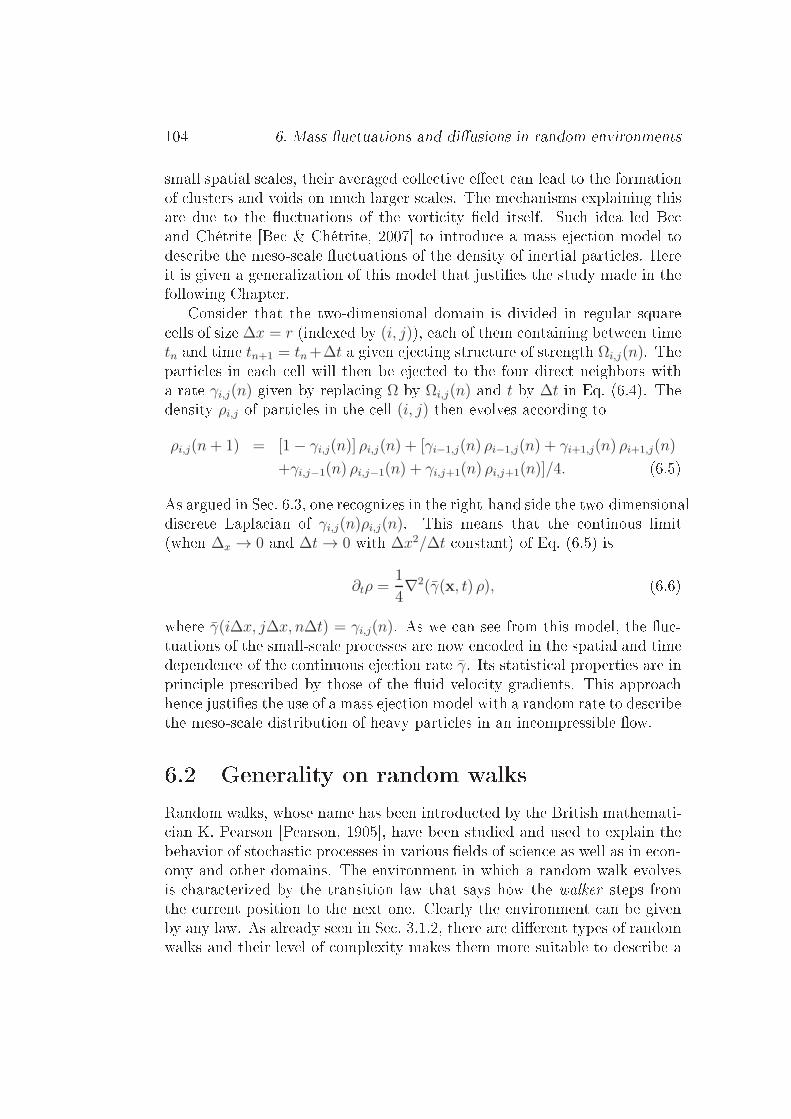
104 6. Mass u tuations and diusions in random environmentssmall spatial s ales, their averaged olle tive ee t an lead to the formationof lusters and voids on mu h larger s ales. The me hanisms explaining thisare due to the u tuations of the vorti ity eld itself. Su h idea led Be and Chétrite [Be & Chétrite, 2007 to introdu e a mass eje tion model todes ribe the meso-s ale u tuations of the density of inertial parti les. Hereit is given a generalization of this model that justies the study made in thefollowing Chapter.Consider that the two-dimensional domain is divided in regular square ells of size ∆x = r (indexed by (i, j)), ea h of them ontaining between timetn and time tn+1 = tn+∆t a given eje ting stru ture of strength Ωi,j(n). Theparti les in ea h ell will then be eje ted to the four dire t neighbors witha rate γi,j(n) given by repla ing Ω by Ωi,j(n) and t by ∆t in Eq. (6.4). Thedensity ρi,j of parti les in the ell (i, j) then evolves a ording toρi,j(n+ 1) = [1− γi,j(n)] ρi,j(n) + [γi−1,j(n) ρi−1,j(n) + γi+1,j(n) ρi+1,j(n)

+γi,j−1(n) ρi,j−1(n) + γi,j+1(n) ρi,j+1(n)]/4. (6.5)As argued in Se . 6.3, one re ognizes in the right-hand side the two-dimensionaldis rete Lapla ian of γi,j(n)ρi,j(n). This means that the ontinous limit(when ∆x → 0 and ∆t → 0 with ∆x2/∆t onstant) of Eq. (6.5) is∂tρ =

1

4∇2(γ(x, t) ρ), (6.6)where γ(i∆x, j∆x, n∆t) = γi,j(n). As we an see from this model, the u -tuations of the small-s ale pro esses are now en oded in the spatial and timedependen e of the ontinuous eje tion rate γ. Its statisti al properties are inprin iple pres ribed by those of the uid velo ity gradients. This approa hhen e justies the use of a mass eje tion model with a random rate to des ribethe meso-s ale distribution of heavy parti les in an in ompressible ow.6.2 Generality on random walksRandom walks, whose name has been introdu ted by the British mathemati- ian K. Pearson [Pearson, 1905, have been studied and used to explain thebehavior of sto hasti pro esses in various elds of s ien e as well as in e on-omy and other domains. The environment in whi h a random walk evolvesis hara terized by the transition law that says how the walker steps fromthe urrent position to the next one. Clearly the environment an be givenby any law. As already seen in Se . 3.1.2, there are dierent types of randomwalks and their level of omplexity makes them more suitable to des ribe a

6.2 Generality on random walks 105pro ess rathen than another. In ase of diusive pro esses in quen hed ran-dom media, one usually applies RWRE te hniques. Many mathemati iansand physi ists have largely investigated RWRE in their dis rete version forsimple reasons of handability in theoreti al studies [Hughes, 1996.Generally one onsiders a latti e with a xed random probability of tran-sition from a site to another and on this setting the behavior of a randomwalk is studied. A lassi referen e for random walks on the integer latti e isthe book [Spitzer, 1976. Mu h work has been dedi ated to a deli ate point,that is to determine the assumptions under whi h RWRE are transient orre urrent. In other words, to establish whether they es ape to innity orindenitely ome ba k to their starting position. For a time-independentrandom environment with no spa e orrelations, it has been shown that therandomization of the environment slowdowns the diusive properties of therandom walk [Solomon, 1975. Furthermore, under some pre ise assump-tions, Y. G. Sinai [Sinai, 1982 proved that one-dimensional nearest-neighborsymmetri random walks (whi h onsist in walkers that an only step be-tween the urrent position and a point in its neighbors, with a symmetri transition probability, i.e. p(x, y) = p(y, x), where x and y are two dierentpositions) in an un orrelated environment are sub-diusive and that, at verylarge time, the position goes likeXt ∼ log2 t, for t → ∞, (6.7)where Xt denotes the position of the walker at time t. In the same yearB, Derrida and Y. Pomeau have demonstrated that when the assumption ofsymmetry is relaxed, the evolution of the position for a random walk followsa power law in time [Derrida & Pomeau, 1982

Xt ∼ tα, (6.8)where the exponent α is greater than zero and smaller than one. Morere ently it was showed that the upper riti al dimension for random walks ina time-independent random environment is equal to 2. Namely, in dimensionsgreater than 2, RWRE are always purely diusive [Bri mont & Kupiainen,1991. In the last de ade important eorts have been also devoted to prove entral-limit theorems or large-deviations prin iples for quen hed disorders[Sznitman, 2004, Zeitouni, 2004, Varadhan, 2004. Generally, it is assumedthat the environment is independent of time and un orrelated in spa e, or atleast with very short spatial orrelations.On the ontrary, mu h less is known in ase of time-dependent environ-ments. One then deals with annealed statisti s (that is a disordered systemdes ribed by random time-dependent variables) where the averages must be

106 6. Mass u tuations and diusions in random environmentsperformed over the u tuations of the random medium. In su h settings andunder some rather general assumptions, it was shown that random walksare always diusive and that entral limit theorems generally hold [Bérard,2004,Dolgopyat et al., 2008.In this part of my thesis the interest is fo used on situations where bothtemporal and spatial s ales of diusion are omparable, or longer, than thoseat whi h the environment u tuates. This is equivalent to have a time-dependent random medium whose temporal and spatial orrelations annotbe negle ted. An instan e where su h settings are relevant is turbulent trans-port. As we have seen in previous se tion, the u tuations of the density inheavy inertial parti le suspensions an be aptured, at least qualitatively, bydiusions in a time-varying random environment. However, also in the aseof simple tra ers, su h an approa h an be relevant. In that ase, most of themodels that are lassi ally used, for example in meteorology and engineering,are based on an eddy-diusivity approa h [Fris h, 1996, whi h in general re-quires a large time-s ale separation between the turbulent u tuations andthe large-s ale variations of the averaged velo ity eld. Advan ed homoge-nization te hniques an be applied to show that the mean on entration eldsatises an ee tive adve tion-diusion equation, with an adve ting velo ityand a diusion oe ient tensor that are dependent on the slow variables de-s ribing the evolution in time and spa e of the average velo ity eld [Goudon& Poupaud, 2004. The mixing at large s ale, originating from u tuationsat small s ales, a ts only through the diusive term. At the same time, asthe solutions to a diusion equation obey a maximum prin iple, the diusiveterm annot be responsible for the reation of large on entrations. There-fore the on entrations observed in ompressible ows an only ome fromthe ee tive adve tion term. As we have seen in Se . 6.1 and as we willfurther dis uss in this hapter, the situation an be somewhat dierent wheninterested in other types of ompressible transport, as for instan e for inertialparti les.6.3 Des ription of the modelWe onsider the dynami s des ribed by the Ito sto hasti dierential equa-tion, dened bydXt =

√2Γσ(Xt, t) dWt, (6.9)where Wt is the lassi al d-dimensional Wiener pro ess, already dis ussedin Se . 3.1.2. We suppose here that the diusion oe ient σ(Xt, t) is arandom, spa e-time dependent eld, whose statisti s are independent of Wt

6.3 Des ription of the model 107as we will see afterwards. Before spe ifying the settings onsidered, it mightbe useful to motivate su h model by onsidering, for instan e, two interestingphysi al problems where Eq. (6.9) arises as a limiting pro ess.As a rst example let us onsider parti les whose dynami s is dissipativein the entire phase spa e and assume that their traje tories obey the NewtonequationXt = Vt, Vt = −µVt +

1√εf

(

Xt, t,t

ε

)

, (6.10)where µ is the Stokes vis ous damping oe ient and ε is a small parameter.Here the ve torial notation is negle ted but still all onsiderations in whatfollows an be easily generalized to any dimension. Equation (6.11) des ribes,for instan e, the dynami s of a heavy inertial parti les in a velo ity eld thatvaries over two dierent time s ales that are separated by a fa tor ε. Inthis equation the for es a ting on the parti le are the vis ous drag and theexternal for e f , whi h depends on spa e and on two dierent time s ales (tand t/ǫ). If we imagine to have a large parti le embedded in a time and spa edependent thermal bath, the fast times ale ε an be interpreted as the typi altime of momentum ex hange between the parti le and its environment. Asin the Einstein original work on Brownian motion, the times ale ε is mu hsmaller than the vis ous damping time 1/µ. In the limit when εµ vanishes,the for e f an be onsidered as a Gaussian noise with orrelationC(t, t′) =

(

1

ε

)⟨

f

(

Xt, t,t

ε

)

f

(

Xt′ , t′,t′

ε

)⟩

ε

≃ 2Γµ2σ2(Xt, t)δ(t− t′),where the average 〈·〉ε is done with respe t to the fast time variable. Thespa e-time variations of σ2 an be interpreted as a non-homogenous temper-ature eld in the thermal bath asso iated to the δ- orrelation in time. Theresulting dynami s is thusXt = Vt, Vt = −µ

[

Vt −√2Γ σ(Xt, t) η(t)

]

, (6.11)where η is the standard white noise.We next onsider the limit when the response time 1/µ is mu h shorterthan the slow time s ale. This introdu es a new fast time s ale O(1/µ) overwhi h the parti le velo ity u tuates. The velo ity orrelation is then givenby〈Vt Vt′〉ε =

t∫

−∞

t′∫

−∞

C(s, s′)eµ(s+s′−t−t′)ds ds′ =

mint,t′∫

−∞

2Γµ2σ2(Xs, s)eµ(2s−t−t′)ds

108 6. Mass u tuations and diusions in random environmentsTherefore, integrating by parts and negle ting exponentially small terms, weobtain〈Vt Vt′〉ε ≈ Γµ σ2(Xmint,t′,mint, t′) e−µ|t−t′|. (6.12)Finally, taking the limit µ → ∞ in Eq. (6.12) we have

〈Vt Vt′〉 = 2Γ σ2(Xt, t)δ(t− t′). (6.13)The parti le position thus satises the sto hasti equation (6.9). The modelthat we are onsidering is thus relevant in studying of Langevin dynami s ina u tuating environment.The se ond situation where Eq. (6.9) appears is in the ontinuous limitof a mass-eje tion model, as we have already forseen in Se . 6.1. To addressthis issue let us onsider a d-dimensional periodi latti e of internode length∆x and period L = N∆x. Naturally, also the time is dis rete and it isexpressed in units of ∆t. Su h a latti e denes a tiling on whi h our dis rete-time dynami s is onsidered. Basi ally, the generi ell indexed by i (withi = 1, 2, . . . , N) ontains at time n∆t a given mass ρi(n). Between two onse utive times n∆t and (n + 1)∆t, a fra tion γi(n) (ranging from 0 to1/(2d)) of su h mass is eje ted from the ell i to one of its 2d neighbors.Clearly the periodi boundary onditions ensure that the total mass M =∑N

i=1 ρi is onserved. For a given set of eje tion rates γi(n)i∈1,...,Nd thevariables ρi(n)i∈1,...,Nd dene a Markov hain whose master equation isgiven byρi(n+ 1) = [1− 2d γi(n)] ρi(n) +

∑

j∈Ni

γj(n)ρj(n), (6.14)where Ni is the number of the neighboring ells of i-th ell and d is a generi dimension. Equation (6.14) des ribes a mass-eje tion pro ess in a time-dependent and non-homogeneous environment determined by the eje tionrates γi(n). It states that the amount of mass ontained in the i-th ell isgiven by the sum of the mass ontained at the previous time, the fra tionγi(n) of mass eje ted and the fra tion of mass oming from the neighboring ells. As already mentioned, a similar model has been studied by [Be &Chétrite, 2007 in the parti ular ase where the environment γi(n) takes onlytwo values, γ or 0, un orrelated in both spa e and time.We now take the eje tion model in Eq. (6.14) and swit h from the dis reteto the ontinuous ase onsiderin the limits ∆x → 0 and ∆t → 0 and, doingthis, we suppose that the ratio ∆x2/∆t = c is kept xed. We denote the ontinous limit of the eje tion rate by

Γσ2(x, t) = lim∆x→0

c γx/∆x(c t/∆x2).

6.4 Statisti al properties of the random environment 109We hoose here σ of the order of unity, so that the oe ient Γ denotes thetypi al amplitude of the eje tion rate. The dimensionless fun tion σ(x, t) isassumed to be time and spa e ontinuous. In this limit, Eq. (6.14) be omes∂ρ(x, t)

∂t= Γ∇2

[

σ2(x, t)ρ(x, t)]

. (6.15)This is the Fokker-Plan k equation asso iated to the Ito sto hasti dierentialEq. (6.9). For a time t > s, we dene the forward transition probabilitydensityp(x, t |y, s) = 〈δ(Xt − x) |Xs = y〉 , (6.16)where 〈·〉 designates averages with respe t to the realizations of the Wienerpro ess Wt. Then the solutions to Eq. (6.15), for all times t greater than s,trivially satisfyρ(x, t) =

∫

p(x, t |y, s) ρ(y, s)dy. (6.17)The model des ribed by the diusion equation Eq. (6.15) an thus be rein-terpreted in terms of a RWRE. Indeed, the dis rete version of the pro essdened by Eq. (6.9) orresponds to a random walk on a d-dimensional latti e,with a probability equal to 2d γi(n) to hop from the i-th site to one of itsneighbors.6.4 Statisti al properties of the random envi-ronment6.4.1 Denition of the random eje tion rateIn the following we spe ify the statisti al properties of the random envi-ronment σ that is used in our model. We onsider d-dimensional periodi settings in a domain of size L = 2π. The environment σ(x, t) is then entirelydetermined in terms of its Fourier series, whi h an be written asσ(x, t) =

∑

|k|

ak χk

(

t

τk

)

eik·x, (6.18)where the ak's are positive real amplitudes and the τk's are s ale-dependent hara teristi times. The Fourier modes χk are su h thatχ−k(t) = χk(t) and χ0 ≡ 0.They are independent Gaussian pro esses with unit varian e and unit or-relation time. The modes χk are hosen as omplex OrnsteinUhlenbe k

110 6. Mass u tuations and diusions in random environmentspro esses that solve the sto hasti dierential equation [Uhlenbe k & Orn-stein, 1930dχk(s) = −χkds+

√2 dBk(s), (6.19)where the Bk's are independent, one-dimensional omplex Wiener pro esses.We now pres ribe some s ale-invarian e properties for the randommedium.Our interest is in environments that satisfy, in a given statisti al sense,

|σ(x+ r, t)− σ(x, t)| ∼ |r|h, (6.20)where h is the lo al Hölder exponent of σ and ontrols, in our ase, theregularity of the eje tion rate. In general h an take any values but it is equalto 0 at points of dis ontinuity, 1 at dierentiable points where σ′ 6= 0 andit is non-negative only if the fun tion is bounded around x. This exponent an be also seen as a sort of lo al s ale in the sense of fra tal geometry(see [Mandelbrot, 1983). Some other onsiderations on the Hölder exponentare reported at the end of this paragraph. We request that the exponent hbeing positive and less than 1. We assume that the Fourier mode amplitudesbehave asak =

1

2|k|− 1

2−h. (6.21)This orresponds to pres ribing that (6.20) is satised for the se ond-ordermoment of the environment in rements.The temporal s ale invarian e is setted by taking τk = |k|−β with β >

0. This latter exponent β relates the time dependen e to the spatial s aleinvarian e; in parti ular when β = 0 the fun tion σ has a single orrelation-time, while when β → ∞ one has a white-noise. As we shall see below, whenh < 1 dimensional analysis will lead to hoose β = 2− 2h.6.4.2 Numeri al methodsIn the numeri al results that are presented hereafter, the averages are per-formed by summing over several realizations of the environment. These re-alizations are obtained by integrating the sto hasti equation (6.19) for theevolution of the mode amplitudes by a standard sto hasti Euler s heme.The time evolution of the mass distribution is obtained in two dierent man-ners, depending on the nature of the question we want to address. A rstapproa h onsists in using an Eulerian s heme that integrates the partialdierential equation (6.15) for the time evolution of the density eld ρ. Forthat we implemented a se ond-order nite-dieren e dis retization for theLapla ian operator and a semi-impli it Euler temporal s heme. This numer-i al s heme ensures the onservation of the total mass with a high a ura y.

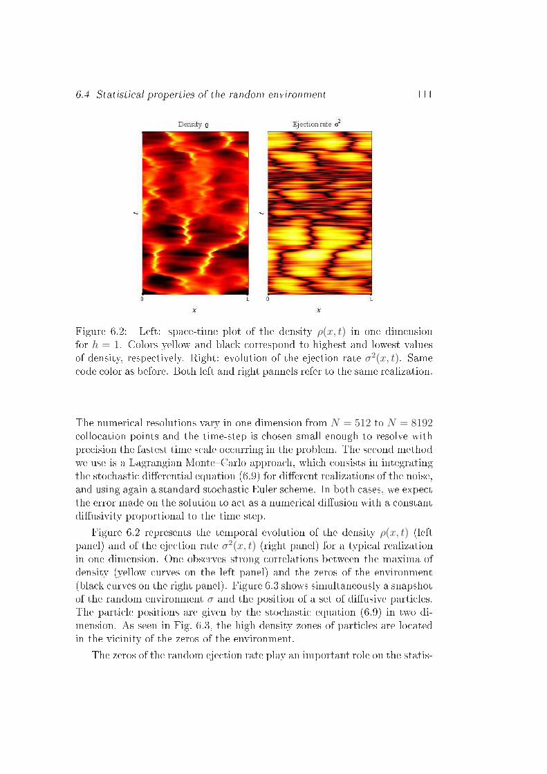
6.4 Statisti al properties of the random environment 111

Figure 6.2: Left: spa e-time plot of the density ρ(x, t) in one dimensionfor h = 1. Colors yellow and bla k orrespond to highest and lowest valuesof density, respe tively. Right: evolution of the eje tion rate σ2(x, t). Same ode olor as before. Both left and right pannels refer to the same realization.The numeri al resolutions vary in one dimension from N = 512 to N = 8192 ollo ation points and the time-step is hosen small enough to resolve withpre ision the fastest time s ale o urring in the problem. The se ond methodwe use is a Lagrangian MonteCarlo approa h, whi h onsists in integratingthe sto hasti dierential equation (6.9) for dierent realizations of the noise,and using again a standard sto hasti Euler s heme. In both ases, we expe tthe error made on the solution to a t as a numeri al diusion with a onstantdiusivity proportional to the time step.Figure 6.2 represents the temporal evolution of the density ρ(x, t) (leftpanel) and of the eje tion rate σ2(x, t) (right panel) for a typi al realizationin one dimension. One observes strong orrelations between the maxima ofdensity (yellow urves on the left panel) and the zeros of the environment(bla k urves on the right panel). Figure 6.3 shows simultaneously a snapshotof the random environment σ and the position of a set of diusive parti les.The parti le positions are given by the sto hasti equation (6.9) in two di-mension. As seen in Fig. 6.3, the high density zones of parti les are lo atedin the vi inity of the zeros of the environment.The zeros of the random eje tion rate play an important role on the statis-

112 6. Mass u tuations and diusions in random environments

Figure 6.3: Snapshot of σ2(x, t) in two dimension and of the parti le positions(green dots) that obey Eq. (6.9). Colors yellow and bla k orrespond tohighest and lowest values of σ, respe tively; thin white lines represent the ontour orrisponding to σ = 0.ti al properties of the mass density and on the parti les diusion properties;this will be further dis ussed throughout this hapter.6.4.3 Phenomenology and dimensionless parametersThe important role of zeros an be heuristi ally understood in the followingway. In ontrast with the standard diusion equation oming from Fi k's rstlaw, the dierential operator ∇2[σ2(x, t) ·], appearing in the right-hand sideof Eq. (6.15), is not positive denite. In su h a ase the maximum prin ipleis not valid and the solution is expe ted to behave very dierently from thoseof lassi al diusion equations. Indeed, the mass gradually a umulates onthe zeros of σ. Suppose that in one dimension σ(x, t) ≃ Cx in the vi inityof x = 0, where C is a given onstant. At leading order, the ux then readsJ = −Γ∂x(σ

2ρ) ≃ −2ΓC2xρ,whi h is positive for x < 0 and negative for x > 0. Thus, there is a permanentux of mass towards the point x = 0. This justies the importan e of hara terizing the zeros, their densities and their lifetimes.

6.4 Statisti al properties of the random environment 113The distribution and time-evolution of the zeros of σ strongly depend onthe dimensionality and on the parameter h. It is lear from the right panelof Fig. 6.2 that the zeros follow random paths in dimension one. We an alsoobserve that for su h a large value of h, that is for a smooth environment,the zeros typi ally appear in pairs and then diuse and separate until theymerge together or with another zero. The diusive behavior of the zeros inone dimension an be explained heuristi ally. For this, let us assume withoutloss of generality that the eje tion rate has only two modes and takes thesimple formσ(x, t) = σr(t) cos x− σi(t) sin x, (6.22)with σr +i σi = 2χ1 (where χ1 denotes the rst Fourier mode). Using the Itoformula it is possible to show that σ an be equivalently rewritten as

σ(x, t) = At sin (x− Φt) , (6.23)where the pro esses At and Φt satisfy the sto hasti equationsdAt = −

(

At −1

At

)

dt+√2 dBA

t , dΦt =

√2

At

dBΦt . (6.24)Here BA

t and BΦt are un orrelated Wiener pro esses. It is lear that theamplitude At u tuates around the value A = 1 and that its orrelation timeis of order one. From Eq. (6.24) it follows that, for typi al values of At, thephase Φt and the position of the zeros of σ diuse on a times ale of the orderof unity. This aspe t will be used later to quantify the mass distribution.As mentioned before, in the parti ular ase in whi h h < 1, the randomenvironment presents s aling properties and thus one expe ts a very dierentbehavior. Indeed, we have that the se ond-order stru ture fun tion of σ, by onstru tion, behaves asδσ2

ℓ = |σ(x, t)− σ(x+ ℓ, t)|2 ∼(

ℓ

L

)2h

. (6.25)The over-line stands for the ensemble average with respe t to the u tuationsof the environment, i.e. with respe t to the OrnsteinUhlenbe k pro esses χk.In this study it has been hoosen to relate the spa e and time orrelationsthrough a dimensional argument. The hara teristi time τk introdu ed inEq. (6.18), behaves as a power law, so that the orrelation time of σ at s aleℓ is

τc(ℓ) =

(

ℓ

L

)β

.

114 6. Mass u tuations and diusions in random environmentsA ording to Eq. (6.25) the diusion times ale asso iated to su h spatials ale ℓ behaves asτd(ℓ) =

ℓ2

Γδσ2ℓ

∼ Γ−1L2hℓ2−2h.The ratio between these two times denes a dimensionless spa e-dependentparameter that is usually alled the Kubo numberKu(ℓ) =

τC(ℓ)

τD(ℓ)≃ ΓL−(2h+β)ℓβ+2h−2. (6.26)When Ku(ℓ) ≫ 1, the environment an be onsidered as frozen whilstfor Ku(ℓ) ≪ 1 it u tuates in an almost time-un orrelated manner. In the ase in whi h β 6= 2− 2h, the Kubo number depends on the s ale ℓ and thisbreaks any possibility of s ale invarian e of the mass distribution. Only when

β = 2− 2h one has that Ku(ℓ) = Ku = Γ/L2 and hen e the s ale invarian eis possible. Here, the fo us is on this latter ase and we will see the mass on entration properties in terms of the dimensionless parameter Ku ∝ Γ.Note that the hoi e of having a s ale-independent Kubo number is ommonin the framework of turbulen e and is expe ted to be relevant to problems ofinertial parti le diusion in turbulent ows.Before moving to next se tion on the diusion properties, let us do someother remarks on the dependen e upon the Hölder exponent h of the envi-ronment. Using Parseval's theorem, it is possible to show that‖σ‖2L2 = ζ(1 + 2h) and ‖∂xσ‖2L2 = ζ(−1 + 2h), (6.27)where ζ(s) is the Riemann zeta fun tion. Thus one has that ‖σ‖L2 < ∞when h > 0 and that ‖∂xσ‖L2 < ∞ when h > 1. Note that at ea h xedtime, σ(x, t) is a Gaussian eld whose in rements have a varian e given byEq. (6.25). Therefore σ(·, t) is a fra tional Brownian motion of exponent

h [Mandelbrot & Ness, 1968. For h = 1/2 it orresponds to the standardBrownian motion. For h > 1/2 the in rements of σ are not independent,their ovarian e is positive and the zeros of σ are nite and isolated. Onthe ontrary, when h < 1/2 the ovarian e of the in rements is negative,therefore we expe t that the number of zeros be ome innite and that theya umulate. As we will see in the next se tions, these dierent behaviors ofthe random environment will ae t the general properties of the diusion.Finally, as the OrnsteinUhlenbe k pro esses χk are stationary, the u -tuations of the eje tion rate σ2 are a stationary and homogeneous randomeld. Hen e one expe ts that, at su iently large times, the density distribu-tion rea hes a statisti ally stationary state and indeed numeri al simulationsindi ate that this is the ase. The results reported here (most of whi h are in

6.5 Diusive properties 115one dimension) mainly on ern the statisti al properties of the density eldin this large-time asymptoti s.6.5 Diusive propertiesFrom now on we will onsider a one-dimensional situation. This se tion on erns the study of the individual traje tories of the Ito sto hasti diusionequation (6.9) in the ases of smooth and non-smooth environments. As wewill see, when the environment σ has a nite orrelation length, parti les arefound to have standard diusion properties at large times with a displa ementdistribution that approa hes that Gaussian.By solving impli itly Eq. (6.9) one obtainsX(t) = X(0) +

√2Γ

∫ t

0

σ(X(s), s) dWs, (6.28)so that⟨

[X(t)−X(0)]2⟩

= 2Γ

∫ t

0

⟨

σ2(X(s), s)⟩

ds, (6.29)where the angular bra kets denote average over all traje tories (that are re-alizations of the Wiener pro ess). At times mu h larger than the orrelationtime of σ2 along parti le traje tories, the integral be omes a sum of indepen-dent random variables, so that the law of large numbers an be applied. Ifthe sto hasti ow dened by Eq. (6.9) is ergodi , one then has〈[X(t)−X(0)]2〉 ∼ 2D(Γ, h) t,with

D(Γ, h) = Γ〈σ2(X(t), t)〉 = Γ

L

∫ L

0

σ2(x, t)ρ(x, t) dx. (6.30)The over-line denotes here the average with respe t to the environment. Theee tive diusion onstant D(Γ, h) involves an average of the environmentalong parti le traje tories, whi h is equivalent in the ase of an ergodi dy-nami s to a spatial average weighted by the density ρ. As we have anti ipated,the traje tories might spend a long time near the zeros of σ. We thus expe tthe Lagrangian average of σ2 to be less than the full Eulerian spatial average.The displa ement u tuations of order less than √t are expe ted to begiven by the entral-limit theorem. However, larger u tuations should obeya large-deviation prin iple with a rate fun tion that might not be purelyquadrati as it is non-trivially related to the Lagrangian properties of theenvironment. To study these u tuations, a Monte-Carlo simulations ofEq. (6.9) is performed.

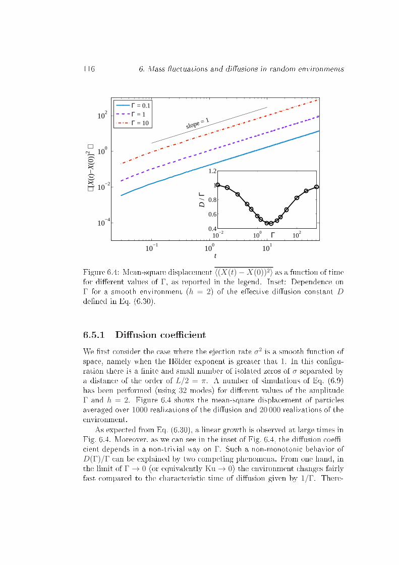
116 6. Mass u tuations and diusions in random environments

10−1

100

101

10−4

10−2

100

102

t

⟨ [X

(t)−

X(0

)]2 ⟩

slope = 1

Γ = 0.1Γ = 1Γ = 10

10−2

100

102

0.4

0.6

0.8

1

1.2

Γ

D /

Γ

Figure 6.4: Mean-square displa ement 〈(X(t)−X(0))2〉 as a fun tion of timefor dierent values of Γ, as reported in the legend. Inset: Dependen e onΓ for a smooth environment (h = 2) of the ee tive diusion onstant Ddened in Eq. (6.30).6.5.1 Diusion oe ientWe rst onsider the ase where the eje tion rate σ2 is a smooth fun tion ofspa e, namely when the Hölder exponent is greater that 1. In this ongu-ration there is a nite and small number of isolated zeros of σ separated bya distan e of the order of L/2 = π. A number of simulations of Eq. (6.9)has been performed (using 32 modes) for dierent values of the amplitudeΓ and h = 2. Figure 6.4 shows the mean-square displa ement of parti lesaveraged over 1000 realizations of the diusion and 20 000 realizations of theenvironment.As expe ted from Eq. (6.30), a linear growth is observed at large times inFig. 6.4. Moreover, as we an see in the inset of Fig. 6.4, the diusion oe- ient depends in a non-trivial way on Γ. Su h a non-monotoni behavior ofD(Γ)/Γ an be explained by two ompeting phenomena. From one hand, inthe limit of Γ → 0 (or equivalently Ku → 0) the environment hanges fairlyfast ompared to the hara teristi time of diusion given by 1/Γ. There-

6.5 Diusive properties 117fore we an imagine that the parti le traje tories sample homogeneously theenvironment, so that the Lagrangian average an be repla ed by the spatialEulerian average. This leads toD(Γ, h) ≃ Γ

L

∫

σ(x, t)2 dx = Γζ(1 + 2h) when Γ → 0. (6.31)For the ase h = 2, we obtain D(Γ, 2)/Γ ≃ 1.03 at small values of Γ, whi h isin agreement with the value observed in the inset of Fig. 6.4. As Γ in reases,the traje tories spend a longer time at the zeros of σ de reasing the valueof D(Γ)/Γ. From the other hand, in the limit of Γ → ∞ (or equivalentlyKu → ∞), the environment an be onsidered ompletely frozen so that themass density, solving Eq. (6.15), is expe ted to be approximately given byρ(x, t) ∼ 1/σ2(x, t). From Eq. (6.30) one nds that

D(Γ, h) =Γ

L

∫

σ2ρ dx ≈ Γ

L

∫

dx = Γ, (6.32)whi h explains why D(Γ)/Γ = 1 at Γ → ∞ (see inset of Fig. 6.4). For su hasymptoti values of Γ the mass is ompletely on entrated at the zeros ofthe eje tion rate and the diusion is arried out by the diusive motionsof the latter. We have indeed seen earlier that in one dimension the zerosdiuse on times ales of the order of unit sin e their dynami s is similar toEq (6.24).6.5.2 PDF of displa ementTo omplete this des ription on the diusive properties in the ase h = 2, letus onsider the normalized probability distribution fun tions (PDFs) of thedispla ements. They are shown in Fig. 6.5. The three panels refer to dierentvalues of Γ (0.1, 1, and 10) and for ea h of them the PDFs for dierent timesare plotted.At early times and for low values of Γ (panel (a)), the PDF's presentexponential tails. The same observation an be done at intermediate times,for larger values of Γ (blue urves in panels (b) and ( )). In all ases, itis lear that the PDFs approa h the Gaussian distribution at the largesttimes. Note that for su iently large values of Γ, some os illations an beobserved in the PDF tails at intermediate times. As we shall see, this is dueto a trapping ee t rising in the zeros of σ(x, t). To larify this point, itis useful to ompare the PDF of the displa ement for dierent values of Γ hosen at the time t∗ su h that〈(X(t∗)−X(0))2〉 = (L/2)2 = π2.

118 6. Mass u tuations and diusions in random environments

−5 0 510

−5

10−4

10−3

10−2

10−1

100

[X(t) − X(0)] / ⟨ [X(t) − X(0)]2 ⟩1/2

PD

F

t = 0.036t = 0.082t = 0.18t = 0.41t = 0.93t = 2.1t = 4.7t = 10Gaussian(a) Γ = 0.1

−6 −4 −2 0 2 4 610

−5

10−4

10−3

10−2

10−1

100

[X(t) − X(0)] / ⟨ [X(t) − X(0)]2 ⟩1/2 P

DF

t = 0.036t = 0.082t = 0.18t = 0.41t = 0.93t = 2.1t = 4.7t = 10Gaussian(b) Γ = 1

−5 0 510

−5

10−4

10−3

10−2

10−1

100

[X(t) − X(0)] / ⟨ [X(t) − X(0)]2 ⟩1/2

PD

F

t = 0.036t = 0.082t = 0.18t = 0.41t = 0.93t = 2.1t = 4.7t = 10Gaussian( ) Γ = 10

−4 −3 −2 −1 0 1 2 3 410

−3

10−2

10−1

100

[X(t*) − X(0)] / (L/2)

PD

F

Γ = 1Γ = 3Γ = 10Γ = 30

(d) t = t∗Figure 6.5: Res aled PDFs of the displa ement X(t) − X(0) in the aseh = 2. Panels (a), (b) and ( ) refer to Γ = 0.1, 1 and 10 respe tively. Forea h panel, olors orrespond to PDFs at dierent times (as labeled) andthe dashed line is the Gaussian PDF of referen e. The initial ondition was hosen in the statisti ally stationary regime. (d) Same for t = t∗ for dierentvalues of Γ. t∗ is dened as the time needed for parti les to travel a distan e omparable to the separation between two zeros of σ, whi h is of the orderof L/2 = π.

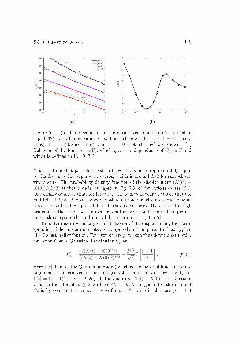
6.5 Diusive properties 119

10−1

100

101

102

10−2

10−1

100

101

102

103

104

105

t

Cp /

A (

Γ)

∝1/t

p = 4p = 6p = 8p = 10

(a) 10−2

10−1

100

101

102

103

1

1.5

2

2.5

3

3.5

4

4.5

5

5.5

ΓA

(Γ)

(b)Figure 6.6: (a) Time evolution of the normalized moments Cp, dened inEq. (6.33), for dierent values of p. For ea h order the ases Γ = 0.1 (solidlines), Γ = 1 (dashed lines), and Γ = 10 (dotted lines) are shown. (b)Behavior of the fun tion A(Γ), whi h gives the dependen e of Cp on Γ andwhi h is dened in Eq. (6.34).t∗ is the time that parti les need to travel a distan e approximately equalto the distan e that separes two zeros, whi h is around L/2 for smooth en-vironments. The probability density fun tion of the displa ement (X(t∗) −X(0))/(L/2) at that time is displayed in Fig. 6.5 (d) for various values of Γ.One learly observes that, for large Γ's, the bumps appear at values that aremultiple of L/2. A possible explanation is that parti les are lose to somezero of σ with a high probability. If they travel away, there is still a highprobability that they are trapped by another zero, and so on. This pi turemight thus explain the multimodal distribution in Fig. 6.5 (d).To better quantify the large-time behavior of the displa ement, the orre-sponding higher-order moments are omputed and ompared to those typi alof a Gaussian distribution. For even orders p, we an thus dene a p-th orderdeviation from a Gaussian distribution Cp as

Cp =〈(X(t)−X(0))p〉

〈(X(t)−X(0))2〉p/2 − 2p/2√πΓ

[

p+ 1

2

]

. (6.33)Here Γ[z] denotes the Gamma fun tion (whi h is the fa torial fun tion whoseargument is generalized to non-integer values and shifted down by 1, i.e.Γ[z] = (z − 1)! [Davis, 1959). If the quantity [X(t) − X(0) is a Gaussianvariable then for all p ≥ 2 we have Cp = 0. More generally, the momentCp is by onstru tion equal to zero for p = 2, while in the ase p = 4 it

120 6. Mass u tuations and diusions in random environments

−10 −5 0 5 1010

−5

10−4

10−3

10−2

10−1

100

[X(t) − X(0)] / ⟨ [X(t) − X(0)]2 ⟩1/2

PD

F

t = 0.034t = 0.17t = 0.87t = 4.4t = 22Gaussian(a) −10 −5 0 5 10

10−5

10−4

10−3

10−2

10−1

100

[X(t) − X(0)] / ⟨ [X(t) − X(0)]2 ⟩1/2

PD

F

t = 0.036t = 0.18t = 0.93t = 4.7t = 24Gaussian(b)Figure 6.7: Res aled probability density fun tion of [X(t)−X(0) at dierenttimes for h = 0.2 (a) and h = 0.6 (b). In both ases Γ = 1. Bla k dashedlines orrespond to the Gaussian distribution. orresponds to the Kurtosis. As seen from Fig. 6.6(a), data suggest that allthe Cp's display a 1/t behavior at large times. The onstant in front of thisbehavior depends of ourse on the amplitude Γ and on the order p. However,the behavior at large times is well tted by a fun tion of the form

Cp ≃A(Γ)λp/2

t, (6.34)where λ is a positive onstant. The temporal evolution of Cp/A(Γ) for dier-ent values of Γ and p, and the fun tion A(Γ) are displayed in Fig. 6.6(a) and6.6(b), respe tively. As seen in Fig. 6.6(a), the data for dierent Γ and for

p xed ollapse at large times. The limiting lines asso iated with dierentorders are equally spa ed, onrming the dependen e in λp/2 of the onstant.The value of λ was found to be λ ≈ 15.Dierent simulations have been performed for various values of the expo-nent h and a behavior similar to the smooth ase was found. For instan e, theparti les diuse at large times and their statisti s be ome Gaussian. Thisis evident from the res aled PDFs of the displa ement shown in Fig. 6.7,for h = 0.2 (a) and h = 0.6 (b), whi h both orrespond to Γ = 1. Also,it has been found that the averaged squared displa ement 〈(X(t)−X(0))2〉presents a linear growth onsistent with Eq. (6.30) (the data is not shownhere). Finally, the diusion oe ient D(Γ, h) was measured as a fun tionof the exponent h and the result is reported in Fig. 6.8. In this plot, whi hrefers to the ase Γ = 1, the divergent behavior of D(Γ, h) at small h is due

6.6 Density u tuations 121

0.2 0.4 0.6 0.8 1 1.2 1.4 1.6 1.8 21

1.1

1.2

1.3

1.4

1.5

1.6

1.7

1.8

h

D

0 0.5 1 1.5 20.5

0.6

0.7

0.8

0.9

1

1.1

1.2

h

D/D

0

Figure 6.8: Behavior of the diusion oe ient D(Γ, h) as a fun tion ofthe exponent h, for Γ = 1. The inset shows the same data normalized byD0 = ‖σ‖2L2.to the divergen e of the L2 − norm of σ(x, t) when h → 0. The inset ofFig. 6.8 shows the trend of the diusion oe ient normalized by the squareL2 − norm of the environment σ

D0 = Γ ‖σ‖2L2 = Γ ζ(1 + 2h).

D(Γ, h)/D0 measures the deviations of the diusion oe ient with respe tto uniformly distributed parti les. The ase D(Γ, h)/D0 ≪ 1 orresponds toan important ontribution from the zeros of σ2 in the integration along theparti le paths. As seen from the inset of Fig. 6.8, for a xed value of Γ, theinuen e of the zeros in reases when h de reases.6.6 Density u tuationsAs previously observed, the spatial u tuations of mass density are orrelatedto the distribution of the zeros of the random environment σ(x, t). More pre- isely, from the diusion-like equation (6.15) (whi h des ribes the evolutionof ρ) we observe that the ux of mass isJ(x, t) = Γ σ(x, t) [2∂xσ(x, t)ρ(x, t) + σ(x, t)∂xρ(x, t)] . (6.35)

122 6. Mass u tuations and diusions in random environmentsThis means that the ux of mass vanishes at the zeros of σ, and hen e thatsu h zeros would a t like sinks on entrating all of the mass if they werenot moving. However, sin e the zeros undergo diusion, they are not able toindenitely on entrate mass and the density saturates in their neighborhood.At the same time, as the total mass is onserved, this on entration pro ess auses the reation of voids in the regions where σ is of the order of 1.Under some homogeneity and ergodi ity assumptions for the dynami s,the probability density fun tion of the mass density an be written asP (ρ) =

d

dρ(measure((x, t) | ρ(x, t) ≤ ρ))

= limT→∞

1

2πT

T∫

0

2π∫

0

δ (ρ(x, t)− ρ) dx dt ≡ limT→∞

PT (ρ), (6.36)where PT (ρ) indi ates the time-averaged distribution of ρ over a time intervalof length T . Understanding this quantity will be the main subje t of nextse tions. As we will see, it strongly depends on the parameters Γ and h. ThePDF of density dened in Eq. (6.36) in terms of a spa e-time average willbe a pre ious tool to examine rst the stationary ase and later to proposea phenomenologi al approa h to treat the non-stationary ase.6.6.1 Smooth random environmentsWe onsider rst the limit when the Kubo number Ku goes to innity, whi h orresponds to an eje tion rate amplitude Γ innitely larger than the inverseof the diusion time of the zeros of σ. This also orresponds to the diusionin a time-stationary environment be ause the fastest times ale is that of themotion of mass. Note that, in the limit of a time-independent environment,no stationary state an be a hieved. Mass will then on entrate in the zerosand at t = ∞ the density will be ome atomi , in the sense that it will be on entrated in points that are exa tly the zeros of σ(x). For su ientlylarge but nite times, as almost all the mass is on entrated around thezeros of σ, the eje tion rate an be rewritten through a Taylor expansion inthe vi inity of these points.Without loss of generality, let us assume that a zero appears at the originx = 0 at the initial time t = 0 and does not move. In this limit Eq. (6.15)redu es to

∂tρ = ΓC2∂2x(x

2ρ), (6.37)where C = dσ/dx|x=0. The hange of time s ales t 7→ s = tΓC2 allows usto set ΓC2 = 1. Moreover we onsider an innite domain and an initial

6.6 Density u tuations 123 ondition whi h is bounded in spa e.ρ(x, 0) =

1 for |x| ≤ 1

0 elsewhere .Equation (6.37) an be integrated analyti ally using the method of hara -teristi s. For x > 0 the hange of variable u(y, t) = e2tρ(x = ey−3t, t) leads tothe homogeneous heat equation that an be easily solved by using the orre-sponding Green fun tion (the solution for x < 0 is obtained by symmetry).One then hasρ(x, t) =

e2t√4πt

∫ ∞

0

exp

[

−(z − log |x| − 3t)2

4t

]

dz

=1

2e2t erfc

[

ln |x|+ 3t

2√t

]

, (6.38)where erfc(z) = 2/√π∫∞

ze−s2ds is the omplementary error fun tion.The time-averaged distribution PT (ρ) dened in Eq. (6.36) an then be al ulated. One has

PT (ρ) =1

2πT

T∫

0

2π∫

0

δ(x− xρ(t))

|∂xρ(x(t), t)|dx dt, (6.39)where xρ(t) is the spa e-time ontour line of the density orresponding to

ρ(xρ(t), t) = ρ. As the omplementary error fun tion is bounded, it is learfrom Eq. (6.38) that this line exists only for t > ln ρ/2. The ontour lines ofρ(x, t) are displayed on Fig. 6.9. One observes that, after transients, all themass is on entrated around the point x = 0.The high-density areas are on entrated in a narrow region of spa e. Thiswill justify the saddle-point approximation used below. Changing variablet 7→ λ = 2t/ ln ρ and introdu ing µ(λ; ρ) = − ln xρ(t)/ ln ρ, after some alge-bra, Eq. (6.39) be omes

PT (ρ) =1

T

√

ln3 ρ

4π

2Tln ρ∫

1

√λ e− ln ρF (λ;ρ)dλ, (6.40)where

F (λ; ρ) = λ+ µ(λ; ρ)− 1

2λ

(

3

2λ− µ(λ; ρ)

)2

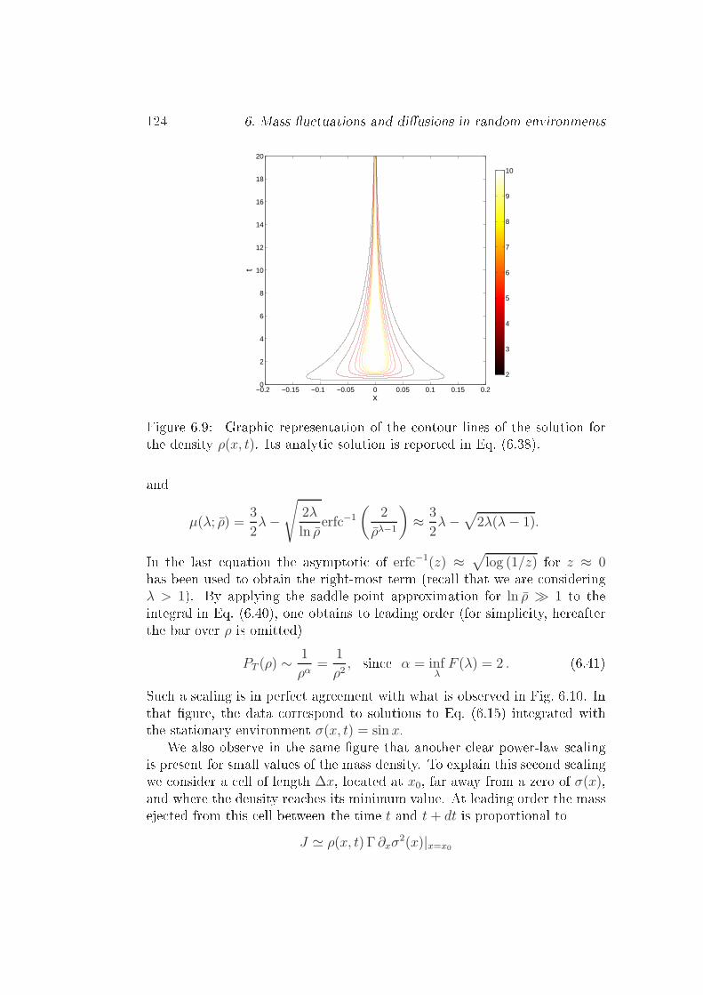
124 6. Mass u tuations and diusions in random environments

x

t

−0.2 −0.15 −0.1 −0.05 0 0.05 0.1 0.15 0.20

2

4

6

8

10

12

14

16

18

20

2

3

4

5

6

7

8

9

10

Figure 6.9: Graphi representation of the ontour lines of the solution forthe density ρ(x, t). Its analyti solution is reported in Eq. (6.38).andµ(λ; ρ) =

3

2λ−

√

2λ

ln ρerfc−1

(

2

ρλ−1

)

≈ 3

2λ−

√

2λ(λ− 1).In the last equation the asymptoti of erfc−1(z) ≈√

log (1/z) for z ≈ 0has been used to obtain the right-most term (re all that we are onsideringλ > 1). By applying the saddle-point approximation for ln ρ ≫ 1 to theintegral in Eq. (6.40), one obtains to leading order (for simpli ity, hereafterthe bar over ρ is omitted)

PT (ρ) ∼1

ρα=

1

ρ2, sin e α = inf

λF (λ) = 2 . (6.41)Su h a s aling is in perfe t agreement with what is observed in Fig. 6.10. Inthat gure, the data orrespond to solutions to Eq. (6.15) integrated withthe stationary environment σ(x, t) = sin x.We also observe in the same gure that another lear power-law s alingis present for small values of the mass density. To explain this se ond s alingwe onsider a ell of length ∆x, lo ated at x0, far away from a zero of σ(x),and where the density rea hes its minimum value. At leading order the masseje ted from this ell between the time t and t + dt is proportional to

J ≃ ρ(x, t) Γ ∂xσ2(x)|x=x0

6.6 Density u tuations 125

10−4

10−2

100

102

10−10

10−8

10−6

10−4

10−2

100

102

104

106

ρ

PD

F

ρ−1

ρ−2

Figure 6.10: Probability distribution fun tion of the density ρ given inEq. (6.36). The PDF seems to display two dierent s aling for large and smallvalues of ρ that are in agreement with Eqs. (6.41) and (6.42), respe tively.Dashed lines highlight these s alings.as ∂xρ ≈ 0 at the point x = x0. Considering that ∂xσ2(x) is onstant near x0yields an exponential de ay of the mass in the ell. Introdu ing in Eq. (6.36) adensity of mass of the form ρ(x, t) ∼ ρ0 e−σ2

0t (where σ2

0 would be an ee tiveeje tion rate) leads toPT (ρ) ∼

1

ρ, (6.42)whi h is in agreement with the left-hand s aling in Fig. 6.10.The situation is rather dierent in the non-stationary ase in whi h themotion of the zeros of the eje tion rate limits the pro ess of mass on entra-tion. As already seen in Se . 6.4, the oe ients σr(t) and σi(t) of Eq. (6.22)are the OrnsteinUhlenbe k pro esses dened in Eqs. (6.18) and (6.19). Theprobability density fun tion of ρ in the non-stationary ase, for an environ-ment with a single mode K = 1 and dierent values of Γ, is displayed inFig. 6.11.The time needed for the density to a umulate near the zero of the eje tionrate σ2 is of the order of Γ−1. Hen e, for small values of Γ (i.e. Ku ≪ 1)the temporal variations of σ(x, t) are very rapid and, as a onsequen e, thesystem does not have mu h time to umulate mass. In this ase it is apparentthat most of the mass is distributed around the mean value 〈ρ〉 = 1 (see

126 6. Mass u tuations and diusions in random environments

10−4

10−3

10−2

10−1

100

101

102

103

10−8

10−6

10−4

10−2

100

102

ρ

PD

F(ρ

)

Γ=0.1

Γ=1

Γ=100

Γ=1000

Γ=10000

0 50 100 150 200

10−5

100

ρ−3/2

Figure 6.11: Log-log plot of the probability density fun tion of the densityρ in the non-stationary ase for K = 1. Dierent olors refer to dierentvalues of Γ. The inset displays the same gure but on a log-lin s ale.orange urve for Γ = 0.1 in Fig. 6.11). However, for large but nite valuesof the Kubo number Ku, the a umulation pro ess is fast enough and theresulting ρ−3/2 s aling is observed. This s aling an be derived by onsideringthat for large Kubo numbers the system qui kly relaxes to a quasi-stationarysolution, in a time of the order of Γ−1, and stays in su h a state for a time omparable to the orrelation time of σ.Depending on how distant we are from a zero, we an have two ases.Far from a zero, the environment behaves as σ(x) ≃ C x, therefore we anoverlook its temporal evolution. In this region, the density onverges to aquasi-stationary solution. The time derivative of ρ is there negligible, so that,to leading order, ∂2

x(σ2ρ) ≈ 0. Hen e one has ρ ≈ σ−2 ∝ 1/x2. In anotherregion, loser to the zero, the time variations of its lo ation be ome fasterthan the on entration of mass and the density saturates to a nite value

ρmax (see the sket h in Fig. 6.12(Left)). The transition between these tworegimes o urs at a distan e ∆x from the zero that, by ontinuity, satisesthe relation∆x ∼ ρ−1/2

max .The length ∆x is of the order of the distan e travelled by the zero during atimes ale equal to that of mass on entration. Hen e, if we assume that thezero diuses, we have that ∆x ∼ Γ−1/2 and the typi al value of ρmax is of theorder of Γ. The distribution of the density has thus a rossover at ρ ∼ Γ. Inthe ase ρ ≪ Γ, whi h o urs for values mu h below the plateau at ρ ≈ ρmax,the behavior is dominated by the divergen e of the quasi-stationary density

6.6 Density u tuations 1272

x

ρmax

x∆

ρt

x∆x

−T

~ 1/ x

Figure 6.12: Left: sket h of the density eld in the vi inity of a zero ofthe eje tion rate σ2 at x = 0. The density grows as x−2 and, at a distan e∆x ∼ ρ

−1/2max of the zero, it rea hes its saturation value ρmax. Right: sket h ofthe diusive time evolution of the position of a zero of σ2. Looking ba kwardbefore the referen e time t = 0, the zero stays at a distan e less than ∆x fora lapse of time T .prole. Repla ing ρ(x) ∼ 1/x2 in Eq. (6.36) one nally obtains

P (ρ) ∼ ρ−3/2 for 1 ≪ ρ ≪ Γ. (6.43)Remarkably, this value of the exponent of the power-law in the intermediatelarge density tail is very robust. It is not shown here but the same behaviorhas also been observed for a larger number of modes and with a dierentenvironment, that is of the form σ(x, t) =√Γ cos (x− ct).The behavior of the PDF of density when ρ ≫ Γ is related to the largeu tuations of ρmax and thus to the events when the zero does not movemu h for a lapse of time larger than Γ−1. More pre isely, if at a xed timewe observe a large value of ρmax, it means that the zero has not moved by adistan e larger than ρ

−1/2max during an interval of time T ; the latter is largerthan Γ−1 as illustrated by the sket h in Fig. 6.12(Right). When the zerosdiuse, this probability is equal to the probability of the rst exit time ofa diusive pro ess. The time T is indeed dened as the rst time whenthe Brownian motion (representing the displa ement of the zero) tou hes abarrier situated at a distan e ∆x from its initial lo ation. The probabilitydensity of the rst time T at whi h the Wiener pro ess exits the interval

|x| < ∆x is ∼ exp(−CT/∆x2) (see, e.g., [Feller, 1971). We thus obtainProb (ρmax > ρ) ∼

∫ ∞

Γ−1

e−C T ρ dT. (6.44)For ρ ≫ Γ the leading-order behavior is given by T = Γ−1. This leads to the

128 6. Mass u tuations and diusions in random environments

10−4

10−2

100

102

10−10

10−5

100

ρ

PD

F

h=0.4h=0.5h=0.6h=0.9h=1.0h=1.1

(a) 10−4

10−2

100

102

10410

−12

10−10

10−8

10−6

10−4

10−2

100

ρ

PD

F

h=0.4h=0.5h=0.6h=0.9h=1.0h=1.1

(b)Figure 6.13: Log-log plot of the PDF of the density ρ in the ase of non-smoooth environment, for Γ = 0.1 (a) and Γ = 10 (b) and dierent values ofh.following exponential uto for the PDF of mass density

P (ρ) ∼ e−C Γ−1 ρ for ρ ≫ Γ. (6.45)This exponential behavior is onrmed numeri ally as an been seen in theinset of Fig. 6.11.6.6.2 Non-smooth random environmentWe ontinue here to analyse the probability density fun tion of the densitybut in the ase of a time-dependent non-smooth eje tion rate σ. Figure 6.13shows the PDF of ρ for dierent values of the exponent h and two values ofΓ, 0.1 and 10. Remark that for large Γ a power-law behavior is observed atsmall masses. The behavior of these tails an be interpreted on the basis ofphenomenologi al arguments similar to those used in [Be & Chétrite, 2007.In this regard, let us onsider an extreme event ausing a very low densityin a ell. We assume that for a long time, mass has only been eje ted fromthis ell. The quantity of matter eje ted per unit time is proportional to themass. This implies that the density is expe ted to display an exponentialde ay and thus to take smal value in a time of the order of T ∝ −Γ−1 ln ρ.Now, let p < 1 be the probability of having su h a onguration, with pthat depends only on the properties of the environment. As the environmentσ de- orrelates in a time of the order of 1, the number n of independent

6.6 Density u tuations 129

0.4 0.6 0.8 10.4

0.6

0.8

1

1.2

1.4

1.6

1.8

2

h

β

Γ=10

Figure 6.14: Fit of the exponent β of the power-law left tails of the PDFsshown in Fig.6.13(b), whi h orresponds to the ase Γ = 10.realizations of σ required for the full pro ess to take pla e during a timeT is proportional to T itself. Hen e one has n ≃ −C Γ−1 ln ρ, where C isa onstant that depends on h. Therefore, the probability of this ompleteevent is

p−C Γ−1 lnρ =(

eln p)−C Γ−1 lnρ

= e− ln pC Γ−1 lnρ = ρ−C Γ−1 ln p,and we obtain that the probability of su h an extreme event is ρβ, withβ = −C ln p/Γ > 0. Note that this is a tually a lower bound to the smallmass tail that is valid as long as p 6= 0 and C 6= 0. Having an analyti expression of the exponent β is a hallenging problem that goes beyond theaim of this study. The exponent β an be a hieved by tting the left tailsof the mass density PDFs within the range where the power-law is observed.These ts are presented in dashed lines in the inset of Fig. 6.13(b) and thedependen e of β on the Hölder exponent h is displayed in Fig. 6.14 for thevalue Γ = 10.Note that the breadths of the PDFs in Fig. 6.13 learly depend on thevalue of the Hölder exponent h as it is apparent on Fig. 6.15 that representsthe varian e of the density δρ2 = 〈(ρ − 〈ρ〉)2〉. The fa t that both theexponent β and the standard deviation δρ do not have a monotoni behavioras a fun tion of h, an be qualitatively explained in the following way. Whenthe value of h de reases, the number of zeros of σ(x, t) in reases. However

130 6. Mass u tuations and diusions in random environments

0.4 0.5 0.6 0.7 0.8 0.9 1 1.10

5

10

15

20

25

30

35

h

δρ2

Γ=0.1

Γ=1

Γ=10

Figure 6.15: Varian e of the density δρ2 = 〈(ρ− 〈ρ〉)2〉 as a fun tion of theexponent h for Γ = 0.1, 1 and 10.the spatial distribution of the zeros also depends on the Hölder exponenth. On the one hand, for h > 1/2 the spa e in rements of σ are positively orrelated. This implies that there is no a umulation of zeros and the massis transported from the zones with non-vanishing values of σ(x, t) to thenearest zeros. Therefore de reasing h from 1 to 1/2, more and more zerosappear reating zones with high mass on entration and, at the same time,void regions. This in reases the density u tuations. On the other hand,for h < 1/2 the ovarian e of in rements is negative and some nite-sizeregions with a large number of zeros appear. In su h zones σ(x, t) vanishesmany times and thus the diusion is very weak. The mass is trapped and itstransfer be omes ine ient, redu ing thus the probability to have extremelylarge or low mass on entrations. In other words, a large number of zerosin reases the density u tuations as long as these zeros are not too dense.The expe ted transition between these two behaviors happens near h = 1/2.This is in agreement with the observed variations of β and δρ2 shown inFigs. 6.14 and 6.15. This behavior is espe ially evident for the largest valueof Γ where the properties of the system are supposed to depend more stronglyon the distribution of zeros of the eje tion rate.

6.7 S ale invarian e of the mass density eld 131

10−2

10−1

100

101

10210

−8

10−6

10−4

10−2

100

PD

F

ρ

(a) h = 2, Γ = 1

10−4

10−2

100

10210

−8

10−6

10−4

10−2

100

PD

Fρ(b) h = 0.5, Γ = 1

10−4

10−2

100

102

10−6

10−4

10−2

100

PD

F

ρ

( ) h = 0.1, Γ = 1

10−4

10−2

100

102

10−8

10−6

10−4

10−2

100

102

ρ

PD

F

l=L

l=L/4

l=L/16

l=L/64

l=L/512

(d) h = 0.5 , various Γ'sFigure 6.16: (a) (b) and ( ) PDFs of the oarse-grained density ρℓ for Γ = 1and three values of the exponent h. Colors orrespond to dierent oarse-graining s ales ℓ hosen of the form ℓ = L/2k with k = 1, . . . 13. In ea h panel,the narrowest urve orresponds to the largest s ale L/2 and the widest urve orresponds to the smallest L/213. The width of the PDF in reases mono-toni ally when the s ale de reases. (d) PDF of the oarse-grained densityρℓ for h = 1/2 and dierent ombinations of Γ and ℓ hosen su h that theee tive rate dened in Eq. (6.48) is onstant.6.7 S ale invarian e of the mass density eldWe nally study the s aling properties of the density eld. In Se . 6.4,we have pres ribed some s ale invarian e properties of the eje tion rate σ.

132 6. Mass u tuations and diusions in random environmentsThe question we want to adress is whether or not and to whi h extent su hproperties translate to the distribution of mass.For that we onsider the oarse-grained mass density, whi h is dened asρℓ(x, t) =

1

ℓ

∫ x+ℓ/2

x−ℓ/2

ρ(y, t) dy. (6.46)By homogeneity we have that 〈ρ〉 = 〈ρℓ〉. The probability density fun tionof the oarse-grained density ρℓ, omputed using the denition in Eq. (6.36),is displayed in Fig. 6.16 for dierent values of h and for Γ = 1. In ea h panelthe PDFs monotoni ally in rease their width when the s ale de reases. Thenarrowest PDF and the widest PDF orrespond to the largest s ale L/2 andthe smallest L/213, respe tively.Comparing the panels, we an see that in ases of spatially smooth envi-ronments, the oarse-grained PDF of mass density be omes gradually invari-ant with respe t to the s ale when h in reases and this is parti ularly evidentin Fig. 6.16(a) for h = 2. This indi ates that the density eld is spatiallysmooth and that the zeros are isolated. Moreover the ollapse is faster forsmall densities be ause the a umulation of mass is weak and o urs only onfew small lusters while the rest of the domain mainly onsists of large voidzones. These large voids dominate the oarse-grained density statisti s up totheir typi al size, whi h is ℓ ≃ L/8, as seen in Fig. 6.16(a). Indeed all urves orresponding to ℓ < L/8 ollapse in the left-hand side of this gure. On the ontrary, the typi al size of mass lusters ℓclust is rather small. Averaging overs ales larger than ℓclust implies the redu tion of the largest mass u tuations.Indeed, the oarse-grained density annot ex eed mclust/ℓ, where mclust is themass aptured by the luster. This uto de reases with ℓ, as an be seen inFig. 6.16(a), allowing less and less u tuations of the oarse-grained density.Su h arguments annot be applied for non-smooth environments wherethe distribution of zeros is more ompli ated. The s ale invarian e is thenbroken, as shown in Figs. 6.16(b) and 6.16( ). This is what an also beseen in Fig. 6.17, whi h displays the varian e of the oarse-grained densityδρ2ℓ = 〈(ρℓ − 〈ρ〉)2〉 as a fun tion of the s ale ℓ for dierent values of h.For h > 1 and ℓ ≪ L the varian e δρ2ℓ does not depend on the s ale ℓ.However, one observes that for h < 1 and ℓ ≪ L the varian e presentsa power-law s aling δρ2ℓ ∼ ℓ−ζ that suggests a self-similar behavior of thedensity. The trend of the power-law exponent ζ(h; Γ) is displayed in theinset of Fig. 6.16( ).To understand the s aling invarian e of the density eld we should look losely to what happens in the neighborhood of the zeros of σ. If we assumethat the eje tion rate vanishes at x = x0, then in the neighborhood of x0, we

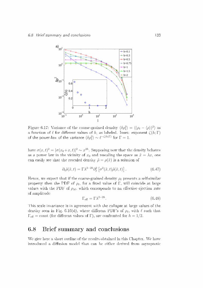
6.8 Brief summary and on lusions 133

10−1

100

101

102

10310

−3

10−2

10−1

100

101

l

δρ2

h=0.1

h=0.3

h=0.5

h=0.75

h=1

h=1.5

h=2

0 1 2

0.2

0.4

0.6

h

ζ(h)

a)

Figure 6.17: Varian e of the oarse-grained density 〈δρ2ℓ〉 = 〈(ρℓ − 〈ρ〉)2〉 asa fun tion of ℓ for dierent values of h, as labeled. Inset: exponent ζ(h; Γ)of the power-law of the varian e 〈δρ2ℓ〉 ∼ ℓ−ζ(h;Γ) for Γ = 1.have σ(x, t)2 = |σ(x0+x, t)|2 ∼ x2h. Supposing now that the density behavesas a power law in the vi inity of x0 and res aling the spa e as x = λx, one an easily see that the res aled density ρ = ρ(x) is a solution of∂tρ(x, t) = Γλ2−2h∂2

x

[

σ2(x, t)ρ(x, t)]

. (6.47)Hen e, we expe t that if the oarse-grained density ρℓ presents a self-similarproperty then the PDF of ρℓ, for a xed value of Γ, will oin ide at largevalues with the PDF of ρλℓ, whi h orresponds to an ee tive eje tion rateof amplitudeΓeff = Γλ2−2h. (6.48)This s ale invarian e is in agremeent with the ollapse at large values of thedensity seen in Fig. 6.16(d), where dierent PDF's of ρℓ, with ℓ su h that

Γeff = const (for dierent values of Γ), are onfronted for h = 1/2.6.8 Brief summary and on lusionsWe give here a short outline of the results obtained in this Chapter. We haveintrodu ed a diusion model that an be either derived from asymptoti

134 6. Mass u tuations and diusions in random environments onsiderations or obtained as the hydrodynami al limit of a simple dis retemass eje tion pro ess where the eje tion rates are random variables withtemporal and spatial orrelations. The model an be interpreted in termsof random walks in a time-dependent random environment. However thesettings are su h that, while the mass is onserved, it does obey a maximumprin iple and the density an be ome arbitrarily large. We have motivatedthis model to study u tuations in turbulent transport.We have onsidered spa e-periodi environments where the temporal de-penden e of ea h Fourier mode is given by independent OrnsteinUhlenbe kpro esses and both the amplitude of the modes and their orrelation timespresent some pres ribed spatial s aling properties. This allowed us to on-sider smooth and non-smooth environments with fast and slow temporaldependen e. No other assumptions were made on the environments and weexpe t them to display generi properties and to be representative of su- iently general situations.The model was studied analyti ally and numeri ally. The orrespondingparti le dynami s is given by an Ito dierential equation with a multipli a-tive noise and no drift. We observed that random traje tories diuse atlarge times. Also, the probability distribution of their displa ements tendsto a Gaussian at large times and the deviations to this asymptoti behaviorde rease as t−1. To take into a ount the u tuations of mass due to the ran-domness of the environment we have introdu ed and studied the probabilitydistribution of the density. We obtained some analyti al results on it in the ase of a stationary environment and we showed that it displays a power-lawtail at large masses with exponent −2. In the general ase, we observeda ompetition between a trapping ee t due to vanishing eje tion rates ofthe random environment and the mixing due to its temporal dependen ethat leads to large u tuations of the density of mass. These u tuationswere studied for both smooth and non-smooth random environment. In thesmooth ase, we showed that the PDF has an intermediate power-law be-havior, like in the stationary ase but with an exponent −3/2 followed by anexponential uto. Finally, we studied the spatial s aling properties of themass distribution by introdu ing a oarse-grained density eld. For smoothrandom environments the oarse-grained density was found to be s ale in-variant. We showed that at large masses, it possesses some s aling propertiesthat depend on the oarse-graining size, the eje tion rate typi al amplitude,and the Hölder exponent of the environment.The overall dynami s of the model proposed in this hapter ontains sev-eral spa e and time s ales. Mass rapidly a umulates near the regions witha vanishing eje tion rate and slowly moves following the diusion of the ze-ros. Depending on the properties of the environment, there is also a lear

6.8 Brief summary and on lusions 135separation of length s ales: small mass u tuations at small s ales and largemass at the s ale between the distan e of two vanishing eje tion rates. Thiss ale separation strongly suggests trying to determine, by standard homoge-nization te hniques, a large-s ale ee tive diusion tensor and eventually anee tive transport term. This issue is kept for future work.Extending our approa h to dimensions higher than one is another possibledire tion for future. The eje tion rate will then vanish on ompli ated setsthat, depending on its regularity, might display fra tal properties. Varyingthe Hölder exponent of the random environment, its amplitude and the ob-servation s ales ould then lead to a rather ri h olle tion of dierent regimes.For instan e, a parti ular attention should be paid to understand whether ornot a power-law is still present in the mass density probability distribution.To on lude, let us stress again that the zeros of the environment play a ru ial role on both the diusive properties and the mass density statisti s.They are responsible for mass a umulation but, at the same time, onstitutebarriers to transport. This duality implies that the ne statisti al details ofsu h systems ru ially depend on the features of the zeros and spe ially onthe lo al stru ture of the eje tion rate in their vi inity. In parti ular thepresen e of an extra drift in the dynami s would ompletely alter the roleof the zeros and would prevent mass a umulation. In this thesis work, wehave de ided to fo us on eje tion rates that an be written as the square ofa generi Gaussian random fun tion. However this hoi e annot be alwaysrelevant and, for instan e, it might be sometimes more appropriate to writethe eje tion rate rather as the exponential of a random fun tion. This would hange drasti ally most of the results showed.

136 6. Mass u tuations and diusions in random environments

Chapter 7Con lusions and perspe tivesIn this hapter we shortly ome ba k to the main results obtained during thisthesis and pla e them in the prospe t of applying them to on rete problemsof atmospheri transport. We naturally distinguish between questions relatedto tra er and passive s alar dynami s and issues where parti le inertia playsa role.Flu tuations of an adve ted on entrationWe have related in Chap. 4 the statisti s of a passive s alar, and in parti ularits spatial orrelations, to the study of the two-point motion of Lagrangiantra ers. Several questions remain open on the work that was presented onthis topi .Firstly, we have studied in Se . 4.4.1 what we alled the lo al dissipation,whi h is dened as the ratio [V ‖]3/R between the ube of the longitudinalvelo ity dieren e and the distan e between two tra ers. We have obtainedunexpe ted eviden e that this quantity attains a s aling regime after a shorttime: its statisti al properties be ome qui kly independent of both time andinitial separations. This suggests that the lo al dissipation is, to leadingorder, statisti ally onserved by the Lagrangian two-point dynami s. How-ever, we have not been able to understand the physi al me hanisms leadingto this behavior. Its average 〈[V ‖]3/R〉r0 over all pairs that are initially at adistan e r0 is initially negative be ause of Kolmogorov's 4/5 law. We foundgeometri al arguments that explain why during Bat helor's ballisti regime,this average rapidly hanges sign and be omes positive. Its onvergen e to a onstant positive value remains unexplained. Identifying the reasons for su ha behavior will have important impa ts on the phenomenon of relative disper-sion and in parti ular on a possible reinterpretation of Ri hardson's explosiveseparation in terms of a purely diusive behavior of velo ity dieren es.Other works on erned the dedu tion of a model for relative dispersion137

138 7. Con lusions and perspe tivesfrom the observation that a eleration dieren es are orrelated over shorttime s ales. As explained in Subse . 4.4.3, the main tool used in this deriva-tion is the entral limit theorem that allowed us to write the time derivativeof velo ity dieren es as a sto hasti pro ess with multipli ative noise. In-terestingly and despite its non-linearity, we argued that the model rea hesat large times a self-similar behavior ompatible with Ri hardson's s aling.However, one of the main short omings of this approa h is the fa t that itmixes phenomenologi al and rigorous arguments in su h a way that the ten-sorial stru ture of a eleration orrelations is not taken into onsiderationand, for the moment, the model is still purely one-dimensional. Extendingit to higher dimensions represents a real hallenge. This would allow us val-idating it more systemati ally against numeri al data and omparing thisapproa h with other realisti sto hasti models. Also, we expe t su h devel-opments to give an alternative way to understand the me hanisms leading toa statisti ally stationary behavior of the lo al dissipation.We now turn to the appli ations of pair dispersion to the study of u tu-ations in turbulent transport. The results obtained in Se s. 5.2 and 5.3 givesome geometri al interpretations of the extreme events that an be observedin the statisti s of distan es between two tra ers. Su h approa hes an beextended to the relative motion of more than two traje tories and in parti u-lar to the time evolution of a blob of Lagrangian tra ers. This would have beof straightforward relevan e to hara terize the dispersion by turbulen e ofa spot of pollutants. We used in Se . 5.3 fra tal geometry onsiderations toquantify the probability that a ouple of tra ers remain at small distan es.One of the plans is to extend this approa h to blobs. This would allow oneto quantify better the probability that a blob keeps a small size or folds to reate on entrations that are mu h higher than those predi ted by eddy-diusivity approa hes. On the ontrary, extremely large separations relateto low on entrations. As we have stressed in Se . 5.2, a violent growth ofthe inter-parti le distan e is explained by a long-time memory of the initialseparation. An extension of these results to the ase of blobs of tra ers isagain of interest. We indeed expe t that su h a study will give lues on howto hara terize the dispersion properties as a fun tion of the initial lo al u -tuations of the turbulent ow. A ertainly too-optimisti obje tive ould beto design a ontrol pro ess for instantaneous pollutant emissions that would hoose release times as a fun tion of ow stru tures in order to optimizedispersion.Finally, let us dis uss to what extent our work applies to pollutant disper-sion in situations that are more generi than the forward-in-time evolutionof pollutant spots. In many interesting ases one is on erned with time- ontinuous sour es. In prin iple, be ause of the linearity of the adve tion-

139diusion equation, su h settings an equivalently be treated as the sum ofseveral instantaneous releases. This superposition prin iple an be used todetermine the evolution of average on entrations from the dynami s of asingle blob. However, when interested in u tuations, that is statisti s witha non-linear dependen e on the on entration (as, e.g., its varian e), theseideas annot be applied. Quantifying u tuations then requires a knowledgeof multi-s ale multi-time orrelations. As a onsequen e, the problem of tur-bulent relative dispersion has to be in prin iple generalized to the full studyof the Lagrangian ow. However, depending on the question of interest, therequired information an be more tra table. For instan e, let us onsidertra ers that are emitted from a point sour e with a onstant rate. Wheninterested in the se ond-order statisti s of the on entration eld, one aneasily see that they relate to the probability that a parti le emitted at atime t1 < t is at time t nearby another parti le, whi h was emitted at atime t2 < t. This probability is dierent from the transition density usedfor relative dispersion, as it requires that the two parti les were at the samelo ation but at dierent times in the past. Clearly, some of the notions thatwere developed and used in this thesis for the lassi al situation of relativedispersion have their equivalent in this analogous problem. However su hextensions would require some eorts.Universality of heavy parti le on entrationsA natural question that arises on the extensions of this thesis work on rela-tive dispersion on erns its validity in the ase of non-ideal parti les. Whenthe transported spe ies have inertia, preferential on entration will ompetewith Ri hardson's dispersion. Previous experimental and numeri al worksuggests that in that ase the explosive law for separation is re overed atsu iently large times [Be et al., 2010,Gibert et al., 2010. However, littleis known about the ee t of inertia on the extreme events of the inter-parti ledistan e. Clearly, the small-s ale lustering of heavy parti les will enhan ethe probability that parti les remain lose together and will strongly ae tthe fra tality observed for small separations between tra ers. For large sep-arations, we have seen that for tra ers, a large initial velo ity dieren e isrequired for them to separate at all times faster than the average. It isknown that su h large velo ity dieren es are even more probable for heavyparti les. This is due to the sling ee t that they are experien ing wheneje ted from vorti es [Falkovi h & Pumir, 2007. One expe ts u tuations tobe again enhan ed by inertia, as these large velo ity dieren es will triggerparti le separation. However, this ee t might be very sensitive to the valueof the Stokes number as the dissipative dynami s of parti les will introdu ea de orrelation of their velo ities on times larger than their response time.

140 7. Con lusions and perspe tivesAll these extensions of relative dispersion to the ase of inertial parti les re-quire analyzing the data of numeri al simulations varying the parti le Stokesnumber and the initial separation in the inertial range.We now give some ideas on the impli ation of the results of Chap. 6 on the on entration properties of heavy parti les. We have motivated the introdu -tion of a random mass eje tion model to des ribe the statisti al properties ofthe distribution of parti les inside the inertial range. We have shown that forsu h models the high on entrations are strongly ae ted by the zeros of theeje tion rate. In parti ular, the latter are responsible for the presen e of apower-law range in the probability distribution of the density. Su h a regimehas not been observed in dire t numeri al simulations of heavy parti les inturbulent ows [Be et al., 2007a. This an be explained by the followingshort oming of the settings in Se . 6.4. Indeed, we have seen in Se . 6.1 thata phenomenologi al estimation of the eje tion rate involves exponentials thatnever vanish. In the model studied later, we have rather written the positiveeje tion rate as the square of a fun tion that generi ally has zeros. It wouldthus be worth extending the results on density u tuations that are reportedin Se . 6.6 to dierent kinds of eje tion rates. This would be parti ularlyuseful to assess whether or not mass eje tion models (or equivalently ran-dom walks in u tuating random environments) an be divided in dierentuniversality lasses and, if this is the ase, to understand to whi h of theminertial parti le dynami s belongs. To nish, it is important to stress thatmass eje tion models an provide a new framework to hara terize parti le on entration in the inertial range of turbulent ows. Classi ally, lusteringproperties are quantied in terms of deviations from the Poisson distributionthat uniformly spread parti les would follow. These deviations, whi h arevery useful in estimating how wrong it is to negle t preferential on entra-tion, do not give mu h information on the nature of the inertial-range parti ledistribution. Designing new observables from simple statisti al physi s mod-els might be helpful. Also, it would be of interest to apply to su h modelsthe approa h in terms of a analysis of the Voronoï mesh that was developedin [Obligado et al., 2011. This ould be useful to understand whether forsu h observables, heavy parti les belong or not to the same universality lassas random diusions in random environments.

Bibliography[A heson, 1990 A heson, D. (1990). Elementary Fluid Dynami s. Oxford:Clarendon Press.[Anselmet et al., 1984 Anselmet, F., Gagne, Y., Hopnger, E., & Antonia,R. (1984). High-order velo ity stru ture fun tions in turbulent shear ows.Journal of Fluid Me hani s, 140, 6389.[Arnéodo et al., 2008 Arnéodo, A., Benzi, R., Berg, J., Biferale, L., Boden-s hatz, E., Busse, A., Calzavarini, E., Castaing, B., Cen ini, M., Chevil-lard, L., et al. (2008). Universal intermittent properties of parti le traje -tories in highly turbulent ows. Physi al review letters, 100(25).[Arya, 1999 Arya, S. (1999). Air pollution meteorology and dispersion. NewYork: Oxford University Press.[Basset, 1888 Basset, A. (1888). A treatise on hydrodynami s: with numer-ous examples, volume 2. Deighton, Bell and Co.[Bat helor, 1950 Bat helor, G. (1950). The appli ation of the similaritytheory of turbulen e to atmospheri diusion. Quarterly Journal of theRoyal Meteorologi al So iety, 76, 133146.[Bat helor, 1952 Bat helor, G. (1952). Diusion in a eld of homogeneousturbulen e. ii. the relative motion of parti le. Mathemati al Pro eedings ofthe Cambridge Philosophi al So iety, 48(02), 345362.[Battaner, 1996 Battaner, E. (1996). Astrophysi al uid dynami s. Cam-bridge: Cambridge University Press.[Be , 2003 Be , J. (2003). Fra tal lustering of inertial parti les in randomows. Physi s of Fluids, 15, L81.[Be et al., 2007a Be , J., Biferale, L., Cen ini, M., Lanotte, A., Musa hio,S., & Tos hi, F. (2007a). Heavy parti le on entration in turbulen e atdissipative and inertial s ales. Physi al review letters, 98(8), 84502.141

142 BIBLIOGRAPHY[Be et al., 2010 Be , J., Biferale, L., Lanotte, A., S agliarini, A., Tos hi,F., et al. (2010). Turbulent pair dispersion of inertial parti les. Journal ofFluid Me hani s, 645, 497528.[Be et al., 2007b Be , J., Cen ini, M., & Hillerbrand, R. (2007b). Cluster-ing of heavy parti les in random self-similar ow. Physi al Review E, 75,025301.[Be & Chétrite, 2007 Be , J. & Chétrite, R. (2007). Toward a phenomeno-logi al approa h to the lustering of heavy parti les in turbulent ows.New Journal of Physi s, 9(3), 77.[Bérard, 2004 Bérard, J. (2004). The almost sure entral limit theorem forone-dimensional nearest-neighbour random walks in a spa e-time randomenvironment. Journal of applied probability, 41(1), 8392.[Bernard et al., 2006 Bernard, D., Boetta, G., Celani, A., & Falkovi h,G. (2006). Conformal invarian e in two-dimensional turbulen e. NaturePhysi s, 2(2), 124128.[Bernard et al., 1996 Bernard, D., Gawedzki, K., & Kupiainen, A. (1996).Anomalous s aling in the n-point fun tions of a passive s alar. Physi alReview E, 54, 2564.[Biferale et al., 2004 Biferale, L., Boetta, G., Celani, A., Devenish, B.,Lanotte, A., & Tos hi, F. (2004). Multifra tal statisti s of lagrangian ve-lo ity and a eleration in turbulen e. Physi al Review Letters., 93, 064502.[Biferale et al., 2005 Biferale, L., Boetta, G., Celani, A., Devenish, B.,Lanotte, A., & Tos hi, F. (2005). Lagrangian statisti s of parti le pairs inhomogeneous isotropi turbulen e. Physi s of Fluids, 17, 115101.[Biferale & Pro a ia, 2005 Biferale, L. & Pro a ia, I. (2005). Anisotropyin turbulent ows and in turbulent transport. Physi s Reports, 414, 43164.[Bitane et al., 2012a Bitane, R., Be , J., & Homann, H. (2012a). Geometryand violent events in turbulent pair dispersion. (submitted to Journal ofTurbulen e), arXiv:1209.2296.[Bitane et al., 2012b Bitane, R., Be , J., & Homann, H. (2012b). Times ales of turbulent relative dispersion. Physi al Review E, 86(4), 045302.[Boetta & E ke, 2012 Boetta, G. & E ke, R. (2012). Two-dimensionalturbulen e. Annual Review of Fluid Me hani s, 44.

BIBLIOGRAPHY 143[Boetta & Musa hio, 2010 Boetta, G. & Musa hio, S. (2010). Eviden efor the double as ade s enario in two-dimensional turbulen e. Physi alReview E, 82, 016307.[Boetta & Sokolov, 2002a Boetta, G. & Sokolov, I. (2002a). Relative dis-persion in fully developed turbulen e: The ri hardson's law and intermit-ten y orre tions. Physi s Review Letters, 88, 094501.[Boetta & Sokolov, 2002b Boetta, G. & Sokolov, I. (2002b). Statisti s oftwo-parti le dispersion in two-dimensional turbulen e. Physi s of Fluids,14, 3224.[Borgas & Yeung, 2004 Borgas, M. & Yeung, P. (2004). Relative disper-sion in isotropi turbulen e. part 2. a new sto hasti model with reynolds-number dependen e. Journal of Fluid Me hani s., 503, 125160.[Bourgoin et al., 2006 Bourgoin, M., Ouellette, N., Xu, H., Berg, J., & Bo-dens hatz, E. (2006). The role of pair dispersion in turbulent ow. S ien e,311(5762), 835.[Boussinesq, 1885 Boussinesq, V. (1885). Sur la résistan e qu'oppose unliquide indéni en repos. In A ad S i, volume 100 (pp. 9357).[Bri mont & Kupiainen, 1991 Bri mont, J. & Kupiainen, A. (1991). Ran-dom walks in asymmetri random environments. Communi ations inmathemati al physi s, 142(2), 345420.[Busse & Müller, 2008 Busse, A. & Müller, W. (2008). Diusion and disper-sion in magnetohydrodynami turbulen e: The inuen e of mean magneti elds. Astronomis he Na hri hten, 329, 714716.[Cardy et al., 2008 Cardy, J., Falkovi h, G., & Gawedzki, K. (2008). Non-equilibrium statisti al me hani s and turbulen e, volume 355. CambridgeUniversity Press.[Castaing et al., 1990 Castaing, B., Gagne, Y., & Hopnger, E. (1990). Ve-lo ity probability density fun tions of high reynolds number turbulen e.Physi a D, 46, 177200.[Celani et al., 2000 Celani, A., Lanotte, A., Mazzino, A., & Vergassola, M.(2000). Universality and saturation of intermitten y in passive s alar tur-bulen e. Physi al Review Letters, 84(11), 23852388.

144 BIBLIOGRAPHY[Charnoz et al., 2011 Charnoz, S., Fou het, L., Aleon, J., & Moreira, M.(2011). Three-dimensional lagrangian turbulent diusion of dust grains ina protoplanetary disk: Method and rst appli ations. The Astrophysi alJournal, 737(1), 33.[Cooper & Alley, 2002 Cooper, C. & Alley, F. (2002). Air pollution ontrol:A design approa h, volume 3rd edition. Waveland Press (Prospe t Heights,IL.).[Csanady, 1973 Csanady, G. (1973). Turbulent diusion in the environment,volume 3. Springer.[Davis, 1959 Davis, P. (1959). Leonhard euler's integral: A histori al proleof the gamma fun tion. The Ameri an Mathemati al Monthly, 66(10),849869.[De Pater & Lissauer, 2001 De Pater, I. & Lissauer, J. (2001). Planetarys ien e. Cambridge University Press.[Dean et al., 2007 Dean, D., Drummond, I., & Horgan, R. (2007). Ee tivetransport properties for diusion in random media. Journal of Statisti alMe hani s: Theory and Experiment, 2007(7), P07013.[Derrida & Pomeau, 1982 Derrida, B. & Pomeau, Y. (1982). Classi al dif-fusion on a random hain. Physi al Review Letters, 48(9), 627630.[Dimotakis, 2005 Dimotakis, P. (2005). Turbulent mixing. Annual Reviewof Fluid Me hani s, 37, 329356.[Dolgopyat et al., 2008 Dolgopyat, D., Keller, G., & Liverani, C. (2008).Random walk in markovian environment. Annals of Probability, 36(5),16761710.[Douady et al., 1991 Douady, S., Couder, Y., & Bra het, M. (1991). Dire tobservation of the intermitten y of intense vorti ity laments in turbu-len e. Physi al review letters, 67(8), 983986.[E kart, 1948 E kart, C. (1948). An analysis of the stirring and mixingpro esses in in ompressible uids. Journal of Marine Resear h, 7, 265275.[Eyink, 2011 Eyink, G. (2011). Sto hasti ux freezing and magneti dy-namo. Physi s Review E, 83, 056405.

BIBLIOGRAPHY 145[Falkovi h et al., 2002 Falkovi h, G., Fouxon, A., & Stepanov, M. (2002).A eleration of rain initiation by loud turbulen e. Nature, 419(6903),151154.[Falkovi h et al., 2001 Falkovi h, G., Gaweedzki, K., & Vergassola, M.(2001). Parti les and elds in uid turbulen e. Reviews of Modern Physi s,73(4), 913975.[Falkovi h & Pumir, 2007 Falkovi h, G. & Pumir, A. (2007). Sling ee t in ollisions of water droplets in turbulent louds. Journal of the Atmospheri S ien es, 64, 44974505.[Faxén, 1922 Faxén, H. (1922). Der widerstand gegen die bewegung einerstarren kugel in einer zähen üssigkeit, die zwis hen zwei parallelen ebenenwänden einges hlossen ist. Annalen der Physik, 373(10), 89119.[Feller, 1971 Feller, W. (1971). An introdu tion to Probability Theory, vol-ume 1 and 2. New York: Wiley.[Fris h, 1996 Fris h, U. (1996). Turbulen e. Cambridge University Press.[Gagne et al., 1990 Gagne, Y., Hopnger, E., & Fris h, U. (1990). A newuniversal s aling for fully developed turbulen e: the distribution of velo -ity in rements. New trends in nonlinear dynami s and pattern-formingphenomena. NATO ASI, 237, 315319.[Gardiner, 1985 Gardiner, C. (1985). Handbook of sto hasti methods forphysi s, hemistry and the natural s ien es, volume 42. Springer.[Gatignol, 1983 Gatignol, R. (1983). Faxen formulae for a rigid parti le in anunsteady non-uniform ow. Journal de Mé anique théorique et appliquée,1(2), 143160.[Gibert et al., 2010 Gibert, M., Xu, H., & Bodens hatz, E. (2010). Inertialee ts on two-parti le relative dispersion in turbulent ows. Europhysi sLetters, 90, 64005.[Gillespie, 1992 Gillespie, D. (1992). Markov pro esses: an introdu tion forphysi al s ientists. A ademi Pr.[Gollub et al., 1991 Gollub, J., Clarke, J., Gharib, M., Lane, B., &Mesquita, O. (1991). Flu tuations and transport in a stirred uid witha mean gradient. Physi al Review Letters, 67, 35073510.

146 BIBLIOGRAPHY[Goudon & Poupaud, 2004 Goudon, T. & Poupaud, F. (2004). Homoge-nization of transport equations: weak mean eld approximation. SIAMJournal on Mathemati al Analysis, 36, 856881.[Grauer et al., 2012 Grauer, R., Homann, H., & Pinton, J.-F. (2012). Lon-gitudinal and transverse stru ture fun tions in high Reynolds-numberturbulen e. New Journal of Physi s, 14, 063016.[Halpin-Healy & Zhang, 1995 Halpin-Healy, T. & Zhang, Y. (1995). Kineti roughening phenomena, sto hasti growth, dire ted polymers and all that.aspe ts of multidis iplinary statisti al me hani s. Physi s Reports, 254,215414.[Harrison & Perry, 1986 Harrison, R. & Perry, R. (1986). Handbook of airpollution analysis, volume 2nd edition. Chapman and Hall, New York.[Homann et al., 2009 Homann, H., Be , J., Fi htner, H., & Grauer, R.(2009). Clustering of passive impurities in magnetohydrodynami tur-bulen e. Physi s of Plasmas, 16, 082308.[Homann et al., 2007 Homann, H., Dreher, J., & Grauer, R. (2007). Impa tof the oating-point pre ision and interpolation s heme on the results ofdns of turbulen e by pseudo-spe tral odes. Computer Physi s Communi- ations, 177(7), 560565.[Howe, 1971 Howe, M. (1971). Wave propagation in random media. Journalof Fluid Me hani s, 45(04), 769783.[Hughes, 1996 Hughes, B. (1996). Random Walks and Random Environ-ments: Random Environments (Vol. 2). Oxford University Press.[Ilyin et al., 2010 Ilyin, V., Pro a ia, I., & Zagorodny, A. (2010). Sto has-ti pro esses rossing from ballisti to fra tional diusion with memory:Exa t results. Physi al Review E, 81, 030105.[Imbrie & Spen er, 1988 Imbrie, J. & Spen er, T. (1988). Diusion of di-re ted polymers in a random environment. Journal of Statisti al Physi s,52, 609626.[Ishihara et al., 2009 Ishihara, T., Gotoh, T., & Kaneda, Y. (2009). Study ofhigh-reynolds number isotropi turbulen e by dire t numeri al simulation.Annual Review of Fluid Me hani s, 41, 165180.

BIBLIOGRAPHY 147[Jayesh & Warhaft, 1991 Jayesh, J. & Warhaft, Z. (1991). Probability dis-tribution of a passive s alar in grid-generated turbulen e. Physi al ReviewLetters, 67, 35033506.[Jullien et al., 1999 Jullien, M., Paret, J., & Tabeling, P. (1999). Ri hardsonpair dispersion in two-dimensional turbulen e. Physi al Review Letter, 82,28722875.[Kolmogorov, 1941a Kolmogorov, A. (1941a). Dissipation of energy in lo- ally isotropi turbulen e. Dokl. Akad. Nauk SSSR, 32, 1618.[Kolmogorov, 1941b Kolmogorov, A. (1941b). The lo al stru ture of turbu-len e in in ompressible vis ous uid for very large reynolds numbers. Dokl.Akad. Nauk SSSR, 30, 913.[Kolmogorov, 1941 Kolmogorov, A. (1941 ). On generation (de ay) ofisotropi turbulen e in an in ompressible vis ous liquid. Dokl. Akad. NaukSSSR, 31, 538540.[Kolmogorov, 1962 Kolmogorov, A. (1962). A renement of previous hy-potheses on erning the lo al stru ture of turbulen e in a vis ous in om-pressible uid at high reynolds number. Journal of Fluid Me hani s, 13,8285.[Koo hesfahani & Dimotakis, 1986 Koo hesfahani, M. & Dimotakis, P.(1986). Mixing and hemi al rea tions in a turbulent liquid mixing layer.Journal of Fluid Me hani s, 170, 83112.[Krai hnan, 1966 Krai hnan, R. (1966). Dispersion of parti le pairs in ho-mogeneous turbulen e. Physi s of Fluids, 9, 19371943.[Krai hnan, 1968 Krai hnan, R. (1968). Small-s ale stru ture of a s alareld onve ted by turbulen e. Physi s of uids, 11, 945953.[Krai hnan, 1971 Krai hnan, R. (1971). Inertial-range transfer in two- andthree-dimensional turbulen e. Journal of Fluid Me hani s, 47(03), 525535.[Krstulovi et al., 2012 Krstulovi , G., Bitane, R., & Be , J. (2012). Dif-fusions in time-dependent random environments: mass u tuations ands aling properties. New Journal of Physi s, 14(7), 073053.[Kurbanmuradov, 1997 Kurbanmuradov, O. (1997). Sto hasti lagrangianmodels for two-parti le trelative turbulent dispersion in high-reynoldsnumber turbulen e. Monte Carlo Methods and Appli ation, 3, 3752.

148 BIBLIOGRAPHY[La Porta et al., 2001 La Porta, A., Voth, G., Crawford, A., Alexander, J.,& Bodens hatz, E. (2001). Fluid parti le a elerations in fully developedturbulen e. Nature, 409, 10171019.[Lewis & Bala, 2006 Lewis, D. & Bala, S. (2006). Plankton predation ratesin turbulen e: A study of the limitations imposed on a predator with anon-spheri al eld of sensory per eption. Journal of Theoreti al Biology,242(44).[Majda & Kramer, 1999 Majda, A. & Kramer, P. (1999). Simplied modelsfor turbulent diusion: theory, numeri al modelling, and physi al phenom-ena. Physi s Reports, 314, 237574.[Mandelbrot, 1983 Mandelbrot, B. (1983). The fra tal geometry of nature.Wh Freeman.[Mandelbrot & Ness, 1968 Mandelbrot, B. & Ness, J. V. (1968). Fra tionalbrownian motions, fra tional noises and appli ations. SIAM Review, 10(4),422437.[Maxey, 1987 Maxey, M. (1987). The gravitational settling of aerosol parti- les in homogeneous turbulen e and random ow elds. Journal of FluidMe hani s, 174, 441465.[Maxey & Riley, 1983 Maxey, M. R. & Riley, J. (1983). Equation of motionfor a small rigid sphere in a nonuniform ow. Physi s of Fluids, 26, 883.[Mezard et al., 1987 Mezard, M., Parisi, G., & Virasoro, M. (1987). SpinGlass Theory and Beyond (World S ienti Le ture Notes in Physi s),volume 9. World S ienti Publishing Company.[Monin & Yaglom, 1971 Monin, A. & Yaglom, A. (1971). Statisti al FluidMe hani s: Me hani s of Turbulen e, volume 1. Cambridge: MIT press.[Mordant et al., 2004 Mordant, N., Crawford, A., & Bodens hatz, E.(2004). Three-dimensional stru ture of the lagrangian a eleration in tur-bulent ows. Physi al Review Letter, 93, 214501.[Obligado et al., 2011 Obligado, M., Missaoui, M., Mon haux, R., Cartel-lier, A., & Bourgoin, M. (2011). Reynolds number inuen e on preferential on entration of heavy parti les in turbulent ows. In Journal of Physi s:Conferen e Series, volume 318 (pp. 052015).

BIBLIOGRAPHY 149[Obukhov, 1941 Obukhov, A. (1941). On the distribution of energy in thespe trum of turbulent ow. Izv. Akad. Nauk SSSR, Ser. Geogr. Geoz., 5,453466.[Opper & Saad, 2001 Opper, M. & Saad, D. (2001). Advan ed mean eldmethods : Theory and pra ti e. MIT Press.[Ott & Mann, 2000 Ott, S. & Mann, J. (2000). An experimental investiga-tion of the relative diusion of parti le pairs in three-dimensional turbulentow. Journal of Fluid Me hani s, 422, 207223.[Ottino, 1989 Ottino, J. (1989). The Kinemati s of Mixing: Stret hing,Chaos and Transport. Cambridge University Press.[Ouellette et al., 2006 Ouellette, N., Xu, H., Bourgoin, M., & Bodens hatz,E. (2006). An experimental study of turbulent relative dispersion models.New Journal of Physi s, 8, 109.[Parisi, 1979 Parisi, G. (1979). Toward a mean eld theory for spin glasses.Physi s Letters A, 73(3), 203205.[Pearson, 1905 Pearson, K. (1905). The problem of the random walk. Na-ture, 72(294), 318342.[Peterson & Dean, 2008 Peterson, R. & Dean, K. (2008). Fore asting ex-posure to vol ani ash based on ash dispersion modeling. Journal of Vol- anology and Geothermal Resear h, 170(34), 230246.[Pilewskie, 2007 Pilewskie, P. (2007). Climate hange: Aerosols heat up.Nature, 448(7153), 541542.[Pinsky & Khain, 1997 Pinsky, M. & Khain, A. (1997). Turbulen e ee tson droplet growth and size distribution in loudsa review. Journal ofAerosol S ien e, 28, 11771214.[Pope, 2000 Pope, S. (2000). Turbulent ows. Cambridge University Press.[Post & Abraham, 2002 Post, S. & Abraham, J. (2002). Modeling the out- ome of drop-drop ollisions in diesel sprays. International Journal ofMultiphase Flow, 28(6), 9971019.[Pumir et al., 2000 Pumir, A., Shraiman, B., & Chertkov, M. (2000). Ge-ometry of lagrangian dispersion in turbulen e. Physi al Review Letters,85, 53245327.

150 BIBLIOGRAPHY[Pumir et al., 1991 Pumir, A., Shraiman, B., & Siggia, E. (1991). Exponen-tial tails and random adve tion. Physi al Review Letters, 66, 29842987.[Rast & Pinton, 2011 Rast, M. & Pinton, J. (2011). Pair dispersion in tur-bulen e: the subdominant role of s aling. Physi al Review Letter, 107,214501.[Ri hardson, 1926 Ri hardson, L. (1926). Atmospheri diusion shown ona distan e-neighbour graph. Pro eedings of the Royal So iety of London.Series A, Containing Papers of a Mathemati al and Physi al Chara ter,110(756), 709737.[Sahimi, 2011 Sahimi, M. (2011). Flow and Transport in Porous Media andFra tured Ro k: From Classi al Methods to Modern Approa hes, volume2nd Edition.[Salazar & Collins, 2009 Salazar, J. & Collins, L. (2009). Two-parti le dis-persion in isotropi turbulent ows. Annual Review of Fluid Me hani s,41, 405432.[Sawford, 2001 Sawford, B. (2001). Turbulent relative dispersion. AnnualReview of Fluid Me hani s, 33(1), 289317.[S atama hia et al., 2012 S atama hia, R., Biferale, L., & Tos hi, F.(2012). Extreme events in the dispersions of two neighboring parti les un-der the inuen e of uid turbulen e. Physi al Review Letters, 109, 144501.[S huma her, 2008 S huma her, J. (2008). Lagrangian dispersion and heattransport in onve tive turbulen e. Physi al Review Letters, 100, 134502.[Seinfeld & Pandis, 2006 Seinfeld, J. & Pandis, S. (2006). Atmospheri hemistry and physi s: from air pollution to limate hange. Somerset,NJ: John Wiley and Sons.[Shaw, 2003 Shaw, R. (2003). Parti le-turbulen e intera tions in atmo-spheri louds. Annual Review of Fluid Me hani s, 35(1), 183227.[She & Lévêque, 1994 She, Z. & Lévêque, E. (1994). Universal s aling lawsin fully developed turbulen e. Physi al Review letters, 72(3), 336339.[Sherrington & Kirkpatri k, 1975 Sherrington, D. & Kirkpatri k, S. (1975).Solvable model of a spin-glass. Physi al Review Letters, 35, 17921796.

BIBLIOGRAPHY 151[Shraiman & Siggia, 1994 Shraiman, B. & Siggia, E. (1994). Lagrangianpath integrals and u tuations in random ow. Physi al Review E, 49,29122927.[Shraiman et al., 2000 Shraiman, B., Siggia, E., et al. (2000). S alar turbu-len e. Nature, 405(6787), 639646.[Sinai, 1982 Sinai, Y. (1982). The limit behavior of a one-dimensional ran-dom walk in a random environment. Teoriya Veroyatnostei i ee Prime-neniya, 27(2), 247258.[Smyth et al., 2001 Smyth, W., Moum, J., & Caldwell, D. (2001). The e- ien y of mixing in turbulent pat hes: inferen es from dire t simulationsand mi rostru ture observations. Journal of physi al o eanography, 31(8),19691992.[Solomon, 1975 Solomon, F. (1975). Random walks in a random environ-ment. The annals of probability, 3(1), 131.[Spitzer, 1976 Spitzer, F. (1976). Prin iples of Random Walks, 2nd edition,volume 34. New-York:Springer-Verlag.[Squires & Eaton, 1991 Squires, K. & Eaton, J. (1991). Preferential on en-tration of parti les by turbulen e. Physi s of Fluids A: Fluid Dynami s,3, 1169.[Sreenivasan, 1991 Sreenivasan, K. (1991). On lo al isotropy of passives alars in turbulent shear ows. Pro eedings of the Royal So iety A Math-emati al Physi al and Engineering S ien es, 434(1890), 165182.[Stevens & Feingold, 2009 Stevens, B. & Feingold, G. (2009). Untanglingaerosol ee ts on louds and pre ipitation in a buered system. Nature,461(7264), 607613.[Stokes, 1850 Stokes, G. (1850). On the ee t of the internal fri tion ofuids on the motion of pendulums, volume IX.[Sznitman, 2004 Sznitman, A. (2004). : (pp. 203266).: Notes of ourse ats hool and Conferen e on Probability Theory, May 2002 - ICTP Trieste.[Tabeling et al., 1996 Tabeling, P., Zo hi, G., Belin, F., Maurer, J., &Willaime, H. (1996). Probability density fun tions, skewness, and atnessin large reynolds number turbulen e. Physi al Review E, 53, 16131621.

152 BIBLIOGRAPHY[Taylor, 1921 Taylor, G. (1921). Diusion by ontinuous movements. Pro- eedings of the London Mathemati al So iety, 20, 196212.[Thomson, 1987 Thomson, D. (1987). Criteria for the sele tion of sto has-ti models of parti le traje tories in turbulent ows. Journal of FluidMe hani s, 180(529-556), 109.[Tos hi & Bodens hatz, 2009 Tos hi, F. & Bodens hatz, E. (2009). La-grangian properties of parti les in turbulen e. Annual Review of FluidMe hani s, 41, 375404.[Uhlenbe k & Ornstein, 1930 Uhlenbe k, G. & Ornstein, L. (1930). On thetheory of the brownian motion. Physi al Review, 36, 823841.[Valavanidis et al., 2008 Valavanidis, A., Fiotakis, K., & Vla hogianni, T.(2008). Airborne parti ulate matter and human health: toxi ologi al as-sessment and importan e of size and omposition of parti les for oxidativedamage and ar inogeni me hanisms. Journal of Environmental S ien eand Health, Part C, 26(4), 339362.[Van Atta & Chen, 1970 Van Atta, C. & Chen, W. (1970). Stru ture fun -tions of turbulen e in the atmospheri boundary layer over the o ean.Journal of Fluid Me hani s, 44, 145159.[Van Kampen, 2007 Van Kampen, N. (2007). Sto hasti pro esses in physi sand hemistry. North Holland.[Varadhan, 2004 Varadhan, S. (2004). Random walks in a random environ-ment. Pro eedings Mathemati al S ien es, 114, 309318.[Wang & Maxey, 1993 Wang, L. & Maxey, M. (1993). Settling velo ity and on entration distribution of heavy parti les in homogeneous isotropi tur-bulen e. Journal of Fluid Me hani s, 256, 2727.[Wang & Pan, 2008 Wang, M. & Pan, N. (2008). Modeling and predi tionof the ee tive thermal ondu tivity of random open- ell porous foams.International Journal of Heat and Mass Transfer, 51(56), 13251331.[Warhaft, 2000 Warhaft, Z. (2000). Passive s alars in turbulent ows. An-nual Review of Fluid Me hani s, 32, 203240.[Yeung & Borgas, 2004 Yeung, P. & Borgas, M. (2004). Relative dispersionin isotropi turbulen e. part 1. dire t numeri al simulations and reynolds-number dependen e. Journal of Fluid Me hani s, 503, 92124.

BIBLIOGRAPHY 153[Yoshimatsu et al., 2009 Yoshimatsu, K., Okamoto, N., S hneider, K.,Kaneda, Y., & Farge, M. (2009). Intermitten y and s ale-dependent statis-ti s in fully developed turbulen e. Physi al Review E, 79, 026303.[Zeitouni, 2004 Zeitouni, O. (2004). Part ii: Random walks in random en-vironment. Le tures on probability theory and statisti s, (pp. 19301930).

Start where you are. Use what you have. Do what you an.- Arthur Ashe -

A knowledgementsFinally I have the pleasure to say thanks to all those people with who I haveshared my do toral experien e in this smiling and sunny Ni e.I am thankful to my advisors Jérémie Be and Alain Noullez for their ontinuous support during my Ph.D. In parti ular, I would like to expressmy gratitude to Jérémie whom, in fa t, very patiently took harge of myentire Ph.D. I really appre iate his expertise, enthusiasm and sense of re-sponsability from whi h I learned very mu h.Besides my advisors, I would like to thank in advan e the rest of the ommittee: A. Lanotte, M. Bourgoin, M.E. Bra het and A. Pumir for hav-ing kindly agreed to be a part of the jury.My sin ere thanks goes also to the guys of my group, Benjamin, Giorgio,Holger, Mamadou and Samriddhi, with whom I had the han e and thepleasure to work and in rease my professional and personal experien e.In parti ular, I am espe ially grateful to Ben, my rst o ial Fren htea her, for helping me to solve all kinds of problems that a person an havein a foreign ountry. It was a pleasure sharing the o e with him and I annot ount the times we spent hatting and laughing over our misadventures! Heis a very generous and good guy and I think I ould not have had a bettero emate.I am also espe ially grateful to Samriddhi-da, a very dear friend. If Ihave been able to deal with all the di ulties of the last part of the Ph.D.it was also thanks to him. I annot explain how mu h he has helped anden ouraged me. Thanks for all of the oees, laughs, amusing squabbles,badminton mat hes, omplaints, jokes, the tedious Bob Dylan songs that Iwas for ed to listen to, ni e emails, lighthearted teasing, gifts, ups of tea,en ouragements, thesis orre tions, Mozart kugeln, bike tours, posta ards, riti isms, dinners, suggestions . . . everything has been very very fun :)

Together with Samriddhi I would also like to say thanks Dario, for thefunny moments and the delightful evenings spent wat hing movies from thetimes of the Puni wars, and Purbasha, for heering me up at distan e!A very very big thanks goes to my wonderful friends and rugby-matesClémen e, Clare, Marion, Naomi (la apitaine), Roxanne et Aurélien (le oa h) for their friendship, whi h has meant to me more than I ould everexpress. I had the han e to share with them a lot of happy and funnymoments (made from 0 up to 2351 m on the sea level) and even the gloryof two well-deserved medals. I will treasure forever these memories. It hasbeen great to know all of them and I am very grateful for all I have re eivedand learned from them in terms of emotions and feelings :)Thanks also to the other rugby-mates Erell, Lila, Marianne, Maud, Sev-erine, and Georges for the fun trainings and the ni e third half times.I wish to thank the people of the internal servi e: Ghislain, Karima,Khaled and Nadia, (the amazing restaurant sta who is the only one inthe world to ombine good ookery and great abaret at the same time);the se retaries Rose and Sylvie; the re eptionists Isabelle and Nathalie (to-gether with the lovely at, Minette); and also Aziz, Christian, David, Fabri e,Françoise, Jean-Maria and Mi hel. Thank you all for the ni e, small daily hats we had and for being always very kind and having time for me.A very spe ial thanks also goes to all of my friends and to my family, halfin Italy and half in Moro o, for supporting me with love for this whole time.To on lude, my greatest and deepest gratitude is for Raaele, withoutwhom none of this would ever have been possible. Indeed this manus riptrepresents the ompletion of a long period of study we have fa ed togethersupporting ea h other. Words are not enough to express what I have insidemy heart but I truly thank him so mu h for everything he gave and did forme in all of these beautiful years.Grazie !