Transit Dosimetry for Patient Treatment Verification with an Electronic Portal Imaging Device

Sean L Berry

Submitted in partial fulfillment of the requirements for the degree of

Doctor of Philosophy in the Graduate School of Arts and Sciences

COLUMBIA UNIVERSITY

2012

© 2012 Sean L Berry

All rights reserved

ABSTRACT

Transit Dosimetry for Patient Treatment Verification with an Electronic Portal Imaging Device

Sean L Berry

The complex and individualized photon fluence patterns constructed during intensity modulated

radiation therapy (IMRT) treatment planning must be verified before they are delivered to the patient.

There is a compelling argument for additional verification throughout the course of treatment due to

the possibility of data corruption, unintentional modification of the plan parameters, changes in patient

anatomy, errors in patient alignment, and even mistakes in identifying the correct patient for treatment.

Amorphous silicon (aSi) Electronic Portal Imaging Devices (EPIDs) can be utilized for IMRT verification.

The goal of this thesis is to implement EPID transit dosimetry, measurement of the dose at a plane

behind the patient during their treatment, within the clinical process. In order to achieve this goal, a

number of the EPID’s dosimetric shortcomings were studied and subsequently resolved.

Portal dose images (PDIs) acquired with an aSi EPID suffer from artifacts related to radiation

backscattered asymmetrically from the EPID support structure. This backscatter signal varies as a

function of field size (FS) and location on the EPID. Its presence can affect pixel values in the measured

PDI by up to 3.6%. Two methods to correct for this artifact are offered: discrete FS specific correction

matrices and a single generalized equation. The dosimetric comparison between the measured and

predicted through-air dose images for 49 IMRT treatment fields was significantly improved (p << .001)

after the application of these FS specific backscatter corrections.

The formulation of a transit dosimetry algorithm followed the establishment of the backscatter

correction and a confirmation of the EPID’s positional stability with linac gantry rotation. A detailed

characterization of the attenuation, scatter, and EPID response behind an object in the beam’s path is

necessary to predict transit PDIs. In order to validate the algorithm’s performance, 49 IMRT fields were

delivered to a number of homogeneous and heterogeneous slab phantoms. A total of 33 IMRT fields

were delivered to an anthropomorphic phantom. On average, 98.1% of the pixels in the dosimetric

comparison between the measured and predicted transit dose images passed a 3%/3mm gamma

analysis.

Further validation of the transit dosimetry algorithm was performed on nine human subjects

under an institutional review board (IRB) approved protocol. The algorithm was shown to be feasible

for patient treatment verification. Comparison between measured and predicted transit dose images

resulted in an average of 89.1% of pixels passing a 5%/3mm gamma analysis. A case study illustrated

the important role that EPID transit dosimetry can play in indicating when a treatment delivery is

inconsistent with the original plan. The impact of transit dosimetry on the clinical workflow for these

nine patients was analyzed to identify improvements that could be made to the procedure in order to

ease widespread clinical implementation.

EPID transit dosimetry is a worthwhile treatment verification technique that strikes a balance

between effectiveness and efficiency. This work, which focused on the removal of backscattered

radiation artifacts, verification of the EPID’s stability with gantry rotation, and the formulation and

validation of a transit dosimetry algorithm, has improved the EPID’s dosimetric performance. Future

research aimed at online transit verification would maximize the benefit of transit dosimetry and greatly

improve patient safety.

i

TABLE OF CONTENTS

List of Tables iv

List of Figures viii

Acknowledgements xiv Chapter 1: General Introduction 1

1.1. The Role of Dosimetric Treatment Verification in Radiation Therapy 2

1.2. A Brief History and Description of the Amorphous Silicon Electronic Portal

Imaging Device 7

1.3. A Motivation for the Use of 2D EPID Dosimetric Treatment Verification 10

1.4. Summary and Organization of the Dissertation 13

Bibliography 14

Chapter 2: A Field Size Specific Backscatter Correction Algorithm for Accurate 20

EPID Dosimetry (Medical Physics 37 (6), June 2010 pp 2425 – 2434)

2.1. Introduction 21

2.2. Method and Materials 22

2.2.a. Quantification of Asymmetry Due to Backscatter 24

2.2.b. Correction and Analysis of Clinically Delivered Fields 29

2.3. Results 30

2.4. Discussion 36

2.5. Conclusion 39

Bibliography 41

Chapter 3: Validation of EPID Positional Stability with Gantry Rotation 43

3.1. Introduction 44

3.2. Method and Materials 45

ii

3.3. Results 46

3.4. Discussion 47

3.5. Conclusion 49

Bibliography 50

Chapter 4: Implementation of EPID Transit Dosimetry Based on a Through-Air

Dosimetry Algorithm (Medical Physics 39 (1), January 2012 pp 87-98) 51

4.1. Introduction 52

4.2. Method and Materials 54

4.2.a. Overview of the Van Esch Pretreatment Through-Air Verification

Algorithm 55

4.2.b. Monte Carlo Simulation to Account for the Addition of Attenuating

Material 56

4.2.c. Measurement of the Detector Response Behind Phantom Material 56

4.2.d. 2DTD Algorithmic Verification 59

4.3. Results 62

4.3.a. Detector Response Behind Phantom Material 62

4.3.b. 2DTD Algorithmic Verification 67

4.4. Discussion 72

4.5. Conclusion 76

Bibliography 77

Chapter 5: Patient Treatment Verification with an EPID Transit Dosimeter 80

5.1. Introduction 81

5.2. Method and Materials 82

5.2.a. Overview of the 2DTD Patient Treatment Verification Algorithm 82

iii

5.2.b. Acquisition and Analysis of Transit PDIs 83

5.3. Results 85

5.3.a. Group Analysis 86

5.3.b. Lung Patient Case Study 90

5.4. Discussion 93

5.5. Conclusion 97

Bibliography 99

Chapter 6: Summary and Conclusion 102

6.1. Summary and Conclusion 103

Bibliography 106

Chapter 7: Suggestions for Future Study 108

7.1. Suggestions for Future Study 109

Bibliography 113

Glossary of Abbreviations and Acronyms 115

iv

LIST OF TABLES

2.1 Summary of the dosimetric comparison results of the measured portal dose image (mPDI),

matrix corrected portal dose image (cPDIm), and generalized equation corrected portal dose

image (cPDIe) with the predicted portal dose image (pPDI) for 10 patients, 49 fields. The first

column represents the anatomical site that the corresponding fields were designed to treat.

The second and third columns represent the collimator setting, in cm, on the target side (Y1)

and gun side (Y2). The fourth column represents the planned anatomical orientation of the

beam using standard abbreviations. For dosimetric purposes all fields were delivered at gantry

= 0°. The mPDI, cPDIm, and cPDIe columns represent the percent area of the image, within the

CIAO, that results in a gamma value greater than 1 when the corresponding image is compared

to the pPDI. The gamma comparison uses a 2%, 2 mm criteria. The “% change” columns

represent the percent change in the area exceeding a gamma value of 1 when one applies a

correction, either matrix (7th column) or equation (last column) based, to the mPDI. A negative

value implies that there is a decrease in the area, so the dosimetric comparison is improved.

The “matrix size” column denotes the size of the correction matrix applied to the mPDI in order

to get the cPDIm. 35

3.1 Tabulation of the offset between the image of the center of the BB and the central EPID pixel.

Negative offset values indicate that the BB projected towards the gun side (inplane) or towards

the X2 jaw side (crossplane) of the central pixel. The total displacement is the square root of the

sum of the squared displacements in the inplane and crossplane directions. 47

4.1 Summary of measurements performed for the commissioning and verification of the 2DTD

algorithm. In the commissioning phase, each field size was delivered through each of the

phantom thicknesses. This data was used to model the central pixel (CP) response. The data for

the largest, 22.2x29.6 cm2, field was also used to model the off-axis pixel (OAP) response.

v

Additional data points for the OAP modeling were acquired through homogeneous slab

thicknesses of 1, 2, and 3 cm. If an open field was used for either commissioning or verification,

300 MU was delivered. IMRT fields used in the verification of the algorithm were delivered with

the MU calculated from the planning system. 58

4.2 Summary of gamma comparison results for the 49 IMRT treatment fields delivered to the flat,

homogeneous phantoms and to the heterogeneous slab phantom shown in Figure 4.1j. A

criteria of 3% of the pPDIair local pixel value and 3 mm was used for the gamma comparison. The

max and min rows correspond to the IMRT field within each phantom irradiation that had the

most and least area, respectively, passing the gamma criteria. The p-value corresponds to the

level of statistical significance in the difference between the results for a given phantom

irradiation versus the through-air (t=0 cm) irradiation using the student’s t-test. 68

4.3 Summary of gamma comparison results for the open 15x15 cm2 fields delivered to the flat,

heterogeneous slab phantoms. A criteria of 3% of the pPDIair local value and 3 mm was used for

the gamma comparison. The identifiers a-j correspond to the phantom schematics shown in

Figure 4.1. While most of the comparisons are very good, the thickness correction fails along

severe, non-anatomical, discontinuities, such as that drawn in Figure 4.1d. 69

4.4 Summary of gamma comparison results for the 33 IMRT fields delivered to the anthropomorphic

phantom. A criteria of 3% of the pPDIair local value and 3 mm was used for the gamma

comparison. The max and min rows correspond to the IMRT field within each irradiation that

had the most and least area, respectively, passing the gamma criteria. The p-value corresponds

to the level of statistical significance in the difference between the results for the

anthropomorphic phantom irradiation versus the through-air irradiation using the student’s t-

test. 71

vi

5.1 Demographic information for the 9 patients who enrolled on the IRB approved transit dosimetry

protocol. Patient 1 was resimulated and replanned partway through treatment and is therefore

listed twice. Only 4 out of 5 of Patient 3’s fields were included in the analysis, as the 5th was

noncoplanar. The two types of IMRT delivery techniques are dynamic multileaf collimation

(DMLC) and step and shoot (SAS). 86

5.2 Measured transit portal dose images (mPDIts) for the same field over each acquired session

were compared using simple percent dose differences (3% and 5%) and gamma analyses (local

3%, 3mm and global 5%, 3mm). These comparisons were then averaged over all of the fields

within a patient and presented above. The statistics for the entire group of patients is

presented in the bottom half of the table. They indicate that a global 5%, 3mm gamma

comparison is a metric that demonstrates stability in the presence of interfraction fluctuations.

87

5.3 Summary of EPID dosimetry results for the entire patient group as well as anatomical subgroups

and delivery techniques. Pre-treatment and transit gamma comparisons between the

respective measured and predicted images are presented for each grouping. The results were

averaged over each patient. The maximum and minimum columns in the table refer to the

patient in each subgroup with the highest or lowest average area passing the gamma criteria.

The column labeled “average” refers to the average of the individual patient averages. The max,

min, and average values reported in the lung subgroup were all the same because there was

only one patient. A student’s t-test was used to report the significance between the differences

in the pre-treatment and transit results. Only trends could be identified due to the small

number of patients in this study. 88

5.4 The gamma comparison results for a subset of beams that definitely did not traverse the

attenuating components of the patient support assembly (PSA) are presented below the results

vii

for all patients and fields. There is approximately a 7% increase in gamma pass rate for this

subset over the entire set of analyzed beams. 89

5.5 Dosimetric verification results for Patient 1 from Table 5.1. Pre-treatment verification was

performed with a local 3%, 3mm criteria, following departmental guidelines (2nd column). A

very poor match using a global 5%, 3mm criteria was observed between prediction and

measurement during the first transit dosimetry session (3rd column). Further investigation

attributed this to internal anatomical changes and a new plan was constructed. The last column

shows the transit verification results for the new plan. These results indicate a much better

consistency between predicted and measured results. 92

viii

LIST OF FIGURES

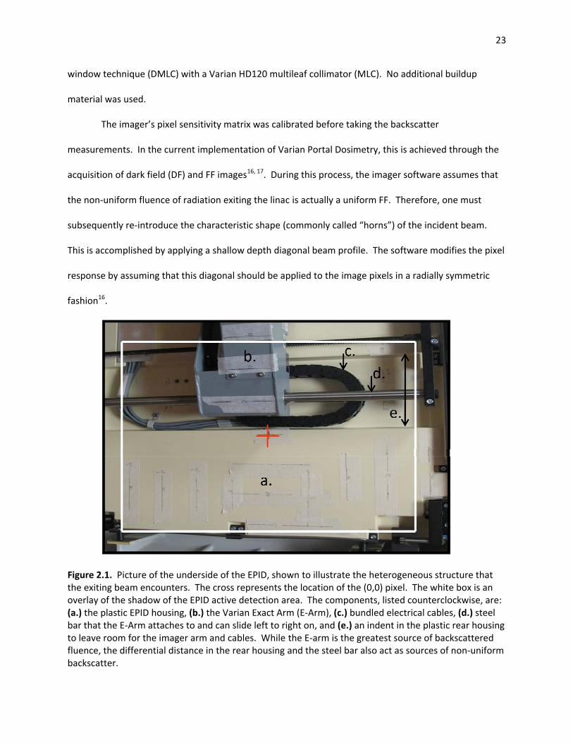
2.1 Picture of the underside of the EPID, shown to illustrate the heterogeneous structure that the

exiting beam encounters. The cross represents the location of the (0,0) pixel. The white box is

an overlay of the shadow of the EPID active detection area. The components, listed

counterclockwise, are: a.) the plastic EPID housing, b.) the Varian Exact Arm (E-Arm), c.)

bundled electrical cables, d.) steel bar that the E-Arm attaches to and can slide left to right on,

and e.) an indent in the plastic rear housing to leave room for the imager arm and cables. While

the E-arm is the greatest source of backscattered fluence, the differential distance in the rear

housing and the steel bar also act as sources of non-uniform backscatter. 23

2.2 a.) The open 5x5 (top row) and 18x18 (bottom row) measured portal dose images (mPDI’s). The

bottom of each image corresponds to the side of the imager closest to the couch (“target side”).

The measured dose on this side is larger than the measured dose on the gun side. b.) The

symmetric portal dose images (sPDI’s) are created by reflecting the gun side of each respective

image about its central row. The excess dose on the target side has been removed and the

displayed dose is symmetric. c.) The correction matrices represent the percent decrease in

dose, on a pixel-by-pixel basis, that needs to be applied to a mPDI to create a sPDI. Note that

the horizontal bands observed in these matrices indicate that the correction occurs principally in

the inplane direction. 25

2.3 a.) 2D line profiles measured along the central column of each field size specific correction

matrix (as shown in Figure 2.2c). The values are shown as data points. The plots start at the (0,

0) pixel and stop 5 mm inside the edge of the collimator jaw on the target side. The solid lines

represent the best linear fit to the data points. The y-intercept of each best fit line is 100%. The

slope of each line is noted and plotted in Figure 2.5. b.) A few of the plots, displayed here as

lighter open shaped data points, and the corresponding linear fits from a.) are shown. These are

ix

combined with profiles measured along a column 1 cm inside of the respective field edge of the

corresponding correction matrices. The off-axis data is plotted as darker closed shaped data

points and labeled “OC”. The graph is limited to a subset of data from a.) for the purposes of

clarity. 27

2.4 2D line profiles measured along a.) the central columns and b.) the columns 1 cm inside of the

respective collimated edge of the measured portal dose images (mPDI’s) (as shown in Figure

2.2a). The absolute dose, in CU, is plotted as a function of absolute inplane distance, in cm,

from the central pixel in that column. The measured dose from the gun side is shown as a solid

line and from the target side is shown as a dotted line. Only a subset of the mPDI’s are

displayed for the purpose of clarity. 28

2.5 The observed slope for each of the best linear fits to the data in Figure 2.4 is plotted as a

function of field size (squares). The data points were modeled by a polynomial of the 4th order

(solid line). A zero slope would indicate that the measured portal dose image (mPDI) was

perfectly symmetric in the inplane direction. 31

2.6 An example of the gamma comparison maps for one of the fields from Table 2.1, “post fossa

rao”. The comparisons between the predicted portal dose image (pPDI) and the a.) measured

portal dose image (mPDI), b.) matrix corrected portal dose image (cPDIm), and c.) generalized

equation corrected portal dose image (cPDIe) are shown. The same field was also delivered to a

MapCHECKTM diode array (Sun Nuclear Corp., Melbourne, Fl) and the corresponding gamma

analysis is shown in d.). The gamma values in the images range from 0 to 1.2. Note that only

the pixels within the irradiated field were counted when calculating the area exceeding a value

of 1. Slight differences may be appreciated between b.) and c.). 35

x

3.1 Imaging phantom that internally contains a 1 mm diameter BB at the intersection of the red

crosshairs. This apparatus attaches rigidly to the end of the patient support assembly and can

be aligned with the linac isocenter using calibrated room lasers. 45

4.1 Heterogeneous phantom geometries. Gray slabs correspond to water equivalent plastic, dotted

slabs correspond to cortical bone equivalent plastic, and white areas correspond to air gaps. All

thicknesses are geometric and given in cm. The diagonal lines indicate the section of the

phantom that was irradiated by the 15 x 15 cm2 field. 60

4.2 An equivalent thickness map through the anthropomorphic phantom calculated at the level of

the EPID detector. Note that the outline indicates the anatomical location of the irradiated

area, which in this example is the thorax. 62

4.3 The MC calculated attenuation of the primary beam CP signal as a function of homogeneous

water equivalent phantom thickness. In order to replicate the physical measurement setup, the

virtual phantom material position was simulated such that the exit surface was 100 cm from the

source and the MC scoring plane was at 135 cm from the source. The first HVL is 14.8 cm and

the second is 16.1 cm. 63

4.4 The EPID measured attenuation along the beam’s CP as a function of homogeneous phantom

thickness. This measurement includes broad beam scatter conditions as well as the detector

dependent response, unlike the primary beam calculation of Figure 4.3. The plots are

normalized such that the measured signal at thickness = 0 cm is 100%. Only a limited set of the

measured FS’s are shown for clarity. The hollowed points represent the measured data and are

replicated in each plot. There is a best-fit exponential attenuation curve, (qt+r)e-μt, for each FS

within a given HVL zone. These zones are highlighted in white in the plots above. In a.) the

curves are optimized to match the data points within the first (0 ≤ t ≤ 15 cm) HVL. Similarly, in

xi

b.) and c.) the curves correspond to the data points within the second (15 < t ≤ 30 cm) and third

(t > 30 cm) HVLs respectively. 63

4.5 The q values from the (qt+r)e-μt fits, examples of which are shown in Figure 4.4, plotted as a

function of field size. The hollowed points represent the measured data. The dark solid lines

represent the best-fit quadratic curves of the form q = α*(FS)2 + β*(FS) + γ. The light dotted

lines represent the 95% confidence interval limits. 64

4.6 mPDIs acquired over the entire imager at 135 cm SDD behind a.) 1 cm, b.) 10 cm, and c.) 30.2

cm of water equivalent phantom material. The axes labels refer to distances scaled to the

isocenter plane. Each image is normalized to a value of 1.0 at its own central pixel. It can be

observed that as the thickness increases, the difference between the OAP and CP values

increases with increasing distance from the CP. Cross-plane line profiles through the center of

the imager are shown in d.) A limited set thicknesses are displayed for the purposes of clarity.

Note that the grid pattern in the images and periodic dips in the line profiles are caused by the

linac couch netting. 64

4.7 The c values from the ∆(x,y,t) = exp-[[x2 + y2]/[ c(t)2]] expression in Equation 4.7, plotted as a

function of homogeneous phantom thickness. The hollowed points represent the measured

data. The dark solid line represents the best-fit power function of the form c(t) = η*t-λ +κ. The

light dotted lines represent the 95% confidence interval limits. The thickness = 1, 2, and 3 cm

data points were important for specifying the appropriate power function. 66

4.8 The EPID measured attenuation along the beam’s CP as a function of homogeneous phantom

thickness. The lines represent data collected for the algorithmic commissioning, where the field

size was defined at the exit surface of the phantom, 100 cm from the source, and the EPID was

at 135 cm SDD. The points represent data collected for the situation where both the phantom

and the EPID were moved further from the beam source, as is more likely to occur in a patient

xii

treatment scenario. For these points, a CS of 10 x 10 cm2, defined at 100 cm from the source,

was used. The location of the data points along the commissioning curves indicates that scaling

the collimator setting to the field size at the phantom exit surface may be an appropriate

method to calculate the correct FS to use in Equation 4.4. 66

4.9 Gamma maps for three of the heterogeneous slab phantom geometries. a.) The 2 cm slab of

bone shown in Figure 4.1f was shown in Table 4.3 to have the greatest area passing the 3%,3mm

criteria, 97.1%. There are no discontinuities in the field. b.) The phantom shown in Figure 4.1i

where the middle layer is half bone (left side) and half air (right side) is a field that represents

the median of the areas passing the gamma criteria, 95.1%. Failure along the junction is

observed. c.) The phantom shown in Figure 4.1d where there is a slab of phantom 5 cm wide

and 24.7 cm tall with just air on either side represents a geometry where the algorithm totally

breaks down. In Table 4.3 only 66.7% of the pixels pass the criteria and these are at the left and

right sides of the field, relatively far from the dual discontinuities. The square pattern on each

image is caused by the beam traversing the netting of the Varian Exact Couch which is

supporting the phantoms. 68

4.10 A sample of the images associated with the transit dose verification for a representative field

from the data in Table 4.4. a.) The Van Esch pPDIair calculated using Eclipse. b.) The mPDIair

acquired with the EPID. The scale is the same for both a.) and b.) and is given in terms of

“Calibrated Units” (CU), Varian’s unit of dose to the EPID. c.) The 3% of local value, 3 mm

gamma evaluation comparing the through-air predicted and measured images. 98.6% of the

pixels passed the gamma criteria. d.) The 2DTD pPDItx created using the calculated thickness

map, the pPDIair in b.), and Equation 4.4. e.) The mPDItx acquired through the anthropomorphic

phantom. The scale is the same for d.) and e.) and is also reported in CU. f.) The gamma

evaluation comparing the through-phantom predicted and measured images. 97.6% of the

xiii

pixels passed the gamma criteria. It is evident that the conversion from the pPDIair in a.) to the

pPDItx in d.) is not a simple rescaling of the dose, rather it also accounts for the effect of the

anthropomorphic phantom’s inhomogeneities. 71

5.1 Representative (global 5%, 3 mm) gamma analysis images for prostate, brain, and lung patients.

The analysis was carried out between measured and predicted transit portal dose images. The

sharp edge in the stripe of failing pixels in the brain field in the second row indicates that part of

the patient support assembly may be interfering with the transit measurement. 89

5.2 Computed tomography (CT) images for Patient 1 from Table 5.1. Corresponding slices from the

original planning CT, a conebeam CT (CBCT) acquired on the linear accelerator immediately

before a treatment session, and the resimulation planning CT are displayed in the first, second,

and third columns respectively. The gross tumor volume (GTV) is delineated in cyan and the

planning target volume (PTV) is drawn in green. The fluid in the posterior aspect of the bilateral

lungs (red arrows) seen in the first column is clearly resolved in the second and third columns.

91

5.3 Representative (global 5%, 3mm) gamma comparison images for Patient 1 from Table 5.1. The

first column shows that large areas of the original plan’s transit dosimetry results exceeded the

gamma threshold. Most of the area of the images in the replan, shown in the second column,

pass the gamma criteria. 92

xiv

ACKNOWLEDGEMENTS

It is only through the support and encouragement of numerous people that the completion of a

Ph.D. program and a doctoral thesis can be accomplished. First and foremost, I would like to thank my

advisor, Cheng Shie Wuu, Ph.D., for his unwavering commitment to my success and to our project.

Rather than objecting to my part time availability, Dr. Wuu made himself available around the clock. He

would host late evening meetings in his office, email during the middle of the night, and call even while

on trips to Taiwan. While this is in general typical of Dr. Wuu’s passion for teaching and mentoring, I am

deeply appreciative.

I would also like to thank the co-authors from our EPID dosimetry publications. Cynthia

Polvorosa is a friend who acted as my eyes, ears, and legs in the Columbia University Department of

Radiation Oncology. She was instrumental to the transit dosimetry protocol in searching out patients

for enrollment and working with the therapists to ensure that they acquired the portal dose images

properly. Rendi Sheu, Ph.D., would run over from Mount Sinai Medical Center for our late evening

meetings, happily lend us his experience and advice on Monte Carlo modeling for radiotherapy planning,

and then run back to finish working late into the night.

The faculty and staff of the Applied Physics and Applied Math department also have my

appreciation. Since we met in 2002, Marlene Arbo has been someone that I know that I could turn to

for help and encouragement. Marco Zaider, Ph.D., was willing to take the time to offer me career and

academic advice even before my admission to Columbia. I am thankful to the members of my thesis

committee, Guillaume Bal, Ph.D., D. Michael Lovelock, Ph.D., Edward Nickoloff, D.Sc., and I. Cevdet

Noyan, Ph.D., for taking the time to read through my work and offer constructive advice and criticism.

Equal thanks and appreciation should be extended to those at Memorial Sloan Kettering Cancer

Center who have enabled me to embark on my career while performing my studies at Columbia. My

deepest appreciation is extended to Margie Hunt. Not only did Margie take a chance in initially hiring

xv

me, a person who at the time had no knowledge of the field of medical physics, but she then

subsequently shepherded me through positions of increasing responsibility. More important in this

context, she has always been an ardent supporter of my graduate education, allowing for flexible work

arrangements so I may attend the necessary classes at Columbia. Howard Amols, Ph.D., and Clif Ling,

Ph.D., were also supportive of my plans to continue my studies while working full time at MSK. I would

also like to thank my current supervisor, Jim Mechalakos, PhD, for his continued support of my

educational goals.

Finally, between work and school, the members of my family are the ones that see me the least

but love me the most. It was only through their patience and support that I had any chance of

completing this thesis. Thank you.

xvi

For my wife,

Rebecca Berry, Ph.D.,

whose support was absolute and confidence in me was unrelenting.

You keep me balanced in life.

1

Chapter 1

General Introduction

2

1.1 THE ROLE OF DOSIMETRIC TREATMENT VERIFICATION IN RADIATION THERAPY

Research activities in medical radiological physics have a rich history that can trace their roots

back to the late 1890’s. This time marks the discovery of x-rays by Wilhelm Röntgen, radioactivity by

Henri Becquerel, and radium by the Curies1. Over the course of the last century, these, and subsequent

findings, are responsible for saving and extending the lives of millions of cancer patients. The World

Health Organization reports that malignant neoplasms are the second leading cause of death worldwide

and the first leading cause of death in developed nations. They comprise 12.6% and 26.6% of all deaths,

respectively2. The American Society for Radiation Oncology (ASTRO) states that, “nearly two-thirds of all

cancer patients will receive radiation therapy during their illness”3. Therefore, research and

development in medical radiological physics is a worthwhile pursuit that has the potential to directly

affect the length and the quality of many lives.

Therapeutic doses of ionization radiation are most typically delivered to patients over a range of

5 to 45 treatment sessions, called fractions. This is done in order to take advantage of radiobiological

differences between malignant and normal cells. Cell kill is a stochastic process and a mechanistic

description is offered by the Linear-Quadratic (LQ) Model4-7. A generalization of the model, where the

surviving fraction (SF) of cells remaining after a total dose, D, of radiation is delivered over n short

exposures punctuated by long intervals where there is time for repair is given by5, 8:

SF = e-βD(α/β + D/n) (1.1)

α and β are constants of proportionality for the linear and quadratic terms respectively9. Typical values

for the α/β ratio are ≥ 10 Gy for tumors and acute normal tissue reactions such as skin erythema and

mucositis and ≤ 3Gy for late normal tissue reactions such as nerve damage, lung fibrosis, and

pneumonitis10. Fractionation exploits this difference between α/β ratios to maximize the therapeutic

ratio, killing the greatest number of malignant cells and sparing as many normal cells as possible.

3

The International Commission on Radiation Units and Measurement (ICRU) has recommended

that the delivered dose be within 5% of the prescribed dose in order to be within the optimal treatment

window11. The American Association of Physicists in Medicine (AAPM), in its report on comprehensive

quality assurance (QA) in radiation oncology, state that this requirement demands that each individual

step in the planning and delivery process must be kept within an accuracy much better than 5%12. This

is challenging for the clinician. A protracted course of radiation implies that the geometric and

dosimetric accuracy of the planned treatment must be maintained over a period of weeks or months.

This includes reproducible patient alignment and positioning with respect to the treatment machine on

a daily basis. Due to their disease, or adjuvant treatments, patients may lose mass, further challenging

the delivered dose’s fidelity to the planned dose. Finally, the constancy of the dose output of the

treatment machine must also be considered over this period.

External beam radiation therapy (EBRT) is most often delivered using a medical linear

accelerator (linac) with accelerating potentials between 4 MV and 25 MV. In photon mode, an electron

beam is accelerated through the waveguide and is then directed into a high atomic number target.

Bremsstrahlung interactions between the electron beam and the target result in a spectrum of x-rays13.

The most typical linac operates at 6 MV, which results in a spectrum of photon energies with a

maximum of approximately 6 MeV and a mean energy near 2 MeV. The angular distribution of

bremsstrahlung photons in this interaction is strongly forward-peaked. Therefore, a flattening filter is

placed in the beam path in order to achieve a relatively uniform intensity over the entire field, which can

project to an area up to 40x40 cm2. The disadvantages of flattening filters are twofold. First, they

absorb 50-90% of the central axis photon intensity13. Second, the beam quality decreases with

increasing radial distance from the central axis (CAX) due to a corresponding decrease in filter

thickness14, 15.

4

The modern era in radiotherapy is characterized by the individualization of radiation treatment

planning (RTP). This is accomplished through the acquisition of a computed tomography (CT) scan for

each patient and computerized treatment planning. CT has the best geometric accuracy when

compared to other imaging modalities, such as magnetic resonance imaging (MRI) or positron emission

tomography (PET). The CT dataset is also used to account for patient’s inhomogeneous internal

composition. The Hounsfield units (HU) within each voxel can be related to the relative electron density

of the corresponding anatomical point. Compton scattering, which depends on a material’s electron

density, is the dominant mode of interaction between the linac’s bremsstrahlung x-rays and human

tissue. This dominance persists over energies ranging from 20 keV to 30 MeV16, which implies that the

CT scan can be used as an accurate patient model for computerized dose calculation. The clinician can

evaluate the merits of a treatment plan by observing the planned dose distribution superimposed on the

patient’s internal anatomy.

The use of inverse planning represents a fundamental development in radiation therapy. The

term “inverse” reflects the fact that, in opposition to traditional planning methods, the desired dose

distribution is the known input and the beam parameters necessary to achieve that distribution are the

output. The planner enters target and critical organ planning goals into an optimization engine. The

optimizer typically uses an objective function that takes the form of a sum of weighted quadratic

functions such as,

Fobj(x) = ∑ wi(di – pi)2) + ∑ ζj · wj(dj – pj)

2) (1.2)

The first sum corresponds to the target where di represents the dose to the ith target point and pi

represents the prescribed dose. The second sum corresponds to the critical organs where dj represents

the dose to the jth critical organ point and pj is the constraint dose. ζj is a flag that notes whether or not

the constraint is being exceeded17. The terms wi and wj allow the user to specify a weight to describe

which constraints are more important than others. The optimizer breaks each individual beam into a

5

large number of sub-beams or beamlets. The optimization engine attempts to find the combination of

individual beamlet weights that minimize the objective function. The resulting dose distributions can

feature good dose conformality about the target. The greatest advantage of this technique over more

conventional methods is the ability to deliver concave dose distributions. This need arises when a target

wraps around a critical organ18.

Intensity Modulated Radiation Therapy (IMRT) is the term for treatments that make use of this

inverse planning approach. The theoretical fluence maps produced by the optimization engine must be

physically deliverable by the linac. One delivery method consists of sliding a number of thin parallel

tungsten shielding leaves continuously across the field at variable speeds while the linac beam is on.

These tungsten leaves constitute a “multileaf collimator” (MLC) and this delivery method is called

dynamic multileaf collimation (DMLC)19, 20. The advantage of DMLC is that it enables both the spatial

and intensity resolutions of the planned and delivered intensity profiles to closely match21. The length

of time that a beam needs to be on in order to deliver the specified dose is given in terms of “monitor

units” (MU). Conventionally, the MU is a function of the linac dose output rate, the prescribed dose, the

size of the field, and the treatment depth22, 23. For DMLC, the MU also is a function of the complexity of

the optimized fluence distribution and the efficiency of the MLC in delivering that fluence pattern. The

intensity profile of any individual beam is not necessarily intuitive and the MU cannot be easily verified

by an independent calculation.

The “black-box” nature of IMRT planning has caused the medical physics and radiation oncology

communities to place emphasis on pre-treatment verification through dosimetric measurements. The

European Society for Therapeutic Radiology and Oncology (ESTRO) state in their Guidelines for the

Verification of IMRT that,

… patient-specific verification was required for IMRT and each plan should be checked prior to delivery. This was different from the conventional approach where checks are generally performed during the commissioning process of a new TPS [treatment planning system] or before the implementation of a new technique…24

6

These recommendations should not be ignored. There have been dire consequences in

instances where pre-treatment patient specific quality assurance (PSQA) was not carried out. One of

the most recent, and most catastrophic, events occurred at Saint Vincent’s Medical Center in New York

City. The DMLC leaf motion instructions became corrupted and did not correspond to the planned dose

distribution shown in the TPS. As a result, the MLC remained completely open rather than sliding across

the field. Since much of the target gets blocked at any given moment, the MU for a DMLC field is

generally 2-5 times greater than that necessary for an open field with uniform fluence. In this case, the

patient’s entire neck from the base of his skull to his larynx had been exposed and severely overdosed.

He subsequently died25. Pre-treatment PSQA would have caught this error.

Historically, pre-treatment PSQA has been performed with an ionization chamber, radiographic

film, and a water equivalent slab phantom26, 27. The dose distribution within the phantom is predicted

by the TPS. The film and chamber are placed within the phantom and the patient’s treatment is

delivered to it. The chamber records the absolute dose and the film records the delivered fluence

pattern. These measurements are compared with prediction. If they sufficiently match, the fluence is

considered deliverable and the fluence transfer from the TPS to the linac has been verified. This method

is effective yet time consuming28. Therefore, alternative methods using arrays of diodes29, arrays of

ionization chambers30, 31, and electronic portal imaging devices32, 33 (EPID’s) have recently been

described. Each collects measured dose data in digital format. Comparisons with the calculated dose

distribution are more convenient and spare the time and expense of radiographic film development.

While pretreatment PSQA is essential, it is not sufficient. Many events can occur between the

time that it is performed and the completion of the patient’s treatment course. Potential technical

issues include major machine malfunctions, user error in linac radiation output calibration, and

subsequent data corruption in the IMRT leaf position instructions. Patient-specific problems may

include wrong positioning, inter-fraction or internal organ motion, and differences in anatomy due to

7

weight or tumor changes. In order to catch these types of errors, the dose delivered during a given

treatment session must be measured. Historically, this has been limited to point dose measurements

using diodes, thermoluminescent diodes (TLD’s), optically stimulated luminescent diodes (OSLD’s), or

metal oxide semiconductor field effect transistors (MOSFET’s). However, points are insufficient in the

era of IMRT since it is highly likely that a mismatch between the measured and expected readings may

be due to a slight misalignment of the dosimeter in the highly modulated field, rather than a problem in

the treatment delivery itself34. Therefore, technologies are currently being developed that are capable

of measuring 2D and 3D isodose distributions. The EPID has shown promise for these types of

measurements35-37.

1.2 A BRIEF HISTORY AND DESCRIPTION OF THE AMORPHOUS SILICON ELECTRONIC PORTAL

IMAGING DEVICE

Electronic portal imaging devices were originally conceived of as a replacement for radiographic

film for patient positional verification38. The digital format of the EPID gives it a number of advantages

over film: no time necessary for development, the data can be accessible from any computer, and

quantitative analysis can be swiftly performed. Adjustment of the image contrast can be done after

acquisition, reducing the need to repeat films in order to highlight specific anatomical details. Modern

EPIDs create an image with significantly less dose than is necessary for film39. The EPID’s integration

with the linac enables the positioning to be performed more quickly and accurately.

While EPID development began in the 1950’s, the technology didn’t mature into

commercialization and widespread use until the late 1980’s. The amorphous silicon (aSi) EPID, popular

today, was originally developed by investigators at the University of Michigan and Xerox PARC in 1987.

It was commercially introduced in 2000 by Varian Medical Systems (Palo Alto, CA) as “Portal Vision

aS500”38. Both the aS500, and its successor the aS1000, are high resolution indirect detectors. The light

emitted from interactions of incident x-rays with an overlying metal plate and scintillating material form

8

the image39-41. The main advantage of this approach over using a direct detector is an order of

magnitude increase in quantum efficiency42, 43.

The aS1000 detector cassette consists of a number of layers, which will be introduced in the

order traversed by the beam44. First is a 9 mm protective layer of circuit board material and Rohacell©,

followed by a 1 mm thick copper buildup plate. Interactions of the incident x-ray beam with this plate

are a source of photoelectrons. X-rays and photoelectrons then hit the gadolinium oxysulfide (Gd2O2S)

phosphor layer. Visible light is released and impinges upon the detection layer. It consists of thin-film

circuitry placed on a 1 mm thick glass substrate. Each image pixel corresponds to a unit consisting of an

aSi photodiode and a thin-film transistor (TFT) switch38. The aS1000 contains an array of 1024x768 pixel

elements, each with a 0.39 mm pitch, resulting in a 40x30 cm2 detection area. The final layer is again

made up of protective materials. The cassette is contained within a larger housing of fiber reinforced

plastic, which is approximately 16 mm thick on the proximal side. While the housing thickness beyond

the cassette is unimportant, its heterogeneity both with respect to composition and distance behind the

cassette influences the quantity of backscattered x-rays into the detector44.

Although designed as an imager, the EPID’s appeal as a dosimeter was quickly appreciated. All

of the stated advantages over traditional film for imaging are also applicable for dosimetry. Numerous

studies have evaluated the aSi EPID’s dosimetric properties. The response is stable, demonstrated to be

within 2% for both short term and long term reproducibility32, 45. Its response is also independent of

dose rate and linear with integrated dose46. For greater than 30 MU, the measured dose is within 2% of

the expected value32. No noteworthy memory effect, where images acquired in one frame carry over

into the next, has been demonstrated for Varian aSi EPIDs45, 47, 48. These features have highlighted the

potential, and increased interest in, the device as a pretreatment, transit, and in vivo dosimeter35.

Despite this increased interest, there has not been a proportional increase in the actual

utilization of EPID dosimetry. Only the simplest dosimetric application, through-air radiation fluence

9

measurement, has been commercialized and widely implemented. The more complex and useful

features, such as transit or in vivo dosimetry, have been relegated to a few major medical centers and

universities35. One reason is that the commercial EPID manufacturers continue to optimize their design

towards radiographic imaging, not dosimetry. The primary aim of that design is to create a usable image

with the least amount of dose. High atomic number components, such as the copper and Gd2O2S layers

described above, are used in order to achieve this goal. This precludes the EPID from behaving as a

tissue equivalent dosimeter. Dosimetric equivalency refers to materials that have the same effective

atomic number (Z), number of electrons per gram, and mass density23. Instead, the EPID displays a

significant energy dependent response, with a hypersensitivity to low energy (< 1 MeV) photons

compared to human tissue 49, 50. This is due to the dominance of the photoelectric effect at these

energies for high Z materials16. Therefore, relating the dose to the EPID to a corresponding dose to

tissue is non-trivial.

EPID dosimetry is also complicated by hardware issues related to the buildup depth and

backscatter. The detection layer is at an approximate water equivalent depth of 8 mm32, which is in the

buildup region of the linac’s megavoltage x-ray beam. In this region, the dose changes rapidly with

depth making it an inconvenient place to acquire data. A number of investigators have asserted that

modifying the hardware to include additional buildup material is preferable for dosimetry. Beyond

moving the measurement point to a more stable depth, it would also theoretically attenuate low energy

scatter originating from the patient40, 51, 52. While this may be true, the focus throughout this entire

thesis is to leave the EPID hardware unmodified in order to allow the results to be widely implemented

throughout the community.

Other proposed hardware modifications include the addition of shielding material to prevent

backscattered radiation from entering the detection layer. The backscatter sources distal of the cassette

include the EPID housing, support arm, positioning motors, and electronic cables53, 54. These materials

10

can contribute to an error of 5-6.5% in the measured dose depending on the field size and position53-55.

Investigations carried out at Columbia University, presented in Chapter 2, use an alternate method

where the backscatter signal as a function of field size and position is identified and corrected for

mathematically56.

Software features, such as the imager calibration procedure, are also deleterious for

dosimetry57. This procedure is designed to account for the individual EPID pixel sensitivities. The most

common technique consists of irradiating the entire imager with the linac beam which is assumed to be

spatially uniform for the purposes of the calibration. Each pixel’s response is adjusted so that it gives a

reading equal to the average value across the imager58, 59. This is a false assumption since the incident

beam intensity changes as a function of radial distance from the central axis due to the linac’s flattening

filter13, 14. Therefore, pixels around the periphery of the detector experience an over-correction. While

this may have a negligible effect for imaging, it must be corrected for dosimetry. To do so, a radial beam

profile measured at a shallow depth is input into the calibration program in order to readjust the pixel

sensitivity setting59.

Although these hardware and software complications exist, they are not insurmountable. The

EPID’s success in the realms of imaging and through-air dosimetry indicate that continued research and

development efforts in transit and in vivo dosimetry are worthwhile.

1.3 A MOTIVATION FOR THE USE OF 2D EPID DOSIMETRIC TREATMENT VERIFICATION

Dosimetric treatment verification may be performed in any number of dimensions. 1D methods

limit the analysis to the dose at a single, or finite number of, points. 2D transit dosimetry techniques

involve comparisons between the calculated or predicted dose in a plane and the measured dose in a

plane. Two common evaluation metrics are the dose difference (DD) and the distance to agreement

(DTA). In the former, the intensity levels between corresponding pixels in the two images are

compared. In the latter, a pixel in the first image is identified and the second image is searched for the

11

nearest pixel with equal intensity. The DD best quantifies the match between two images if the dose

distribution is uniform. However, in areas of high modulation where dose gradients can reach

10%/mm60, the DTA more accurately describes the match. Therefore, hybrid evaluations of delivered

plan quality accounting for both the DD and DTA have been proposed. The gamma index comparison is

the most common and takes the form61:

γ(rm) = min (sqrt[(r2(rm, rc)/∆d2M) + (δ2(rm, rc)/∆D2

M)]) (1.3)

where ∆dM and ∆DM are the user defined DTA and DD criteria respectively. The term r is the distance

and δ is the dose difference between the pixel of interest in the reference image (rc) and the pixel being

evaluated in the measured image (rm). For each rc, one searches the space of the measured image to

find the pixel that minimizes this expression. By definition, the comparison “passes” if γ ≤ 1 using the

user specified criteria, else it fails.

The strength of a 2D technique is that a delivered field’s quality can be described by a single

quantitative value, namely the percentage of the image that passes the gamma index criterion. The

availability of fast and actionable data is essential in a busy radiation oncology clinic. However, a major

weakness of 2D comparisons is that they simply identify whether there is a pass or a fail. One cannot

directly associate a failure with the corresponding dosimetric impact upon the patient. Therefore, some

investigators are proponents of 3D dosimetric evaluations. These may have the benefit of relating

discrepancies from the planned dose with their location in the patient’s anatomy35, 62-64. The delivered

fields are measured by the EPID and that information is combined with a CT of the patient to calculate

the delivered dose distribution. The efficacy of this technique is determined by the fidelity of that CT

model to the actual patient anatomy and position. The use of a scan acquired at the time of treatment,

such as a cone-beam CT (CBCT)65, would be preferable over the planning scan, which could have been

acquired weeks earlier. However, standard CBCT scans acquired before treatment are not necessarily

representative of the patient’s internal anatomy during the beam on time, due to intrafraction motion66-

12

68. This has led to some skepticism in the literature. Gardner, et al. state that “blind application of back-

projection to determine incident fluence is not justified... Dose recalculation based on this false incident

fluence could potentially result in a poorer prediction of the patient dose than making no correction at

all”69. Further, daily CBCT may not be appropriate for treatments delivered over tens of fractions due to

dose considerations. Ding, et al., found that “Doses to radiosensitive organs can total 300 cGy accrued

over an entire treatment course if kV CBCT scans are acquired daily”70. Hyer, et al. found that effective

doses of about 130-286 mSv are possible over a 30 fraction treatment, dependent upon the

manufacturer and standard imaging protocol used71. Even if one neglects the positioning and dose

considerations, daily acquisition of the CBCT and subsequent analysis of the dose distribution may be

prohibitively expensive in terms of information processing time and manpower36.

Since 2D EPID transit dosimetry methods save both dose and time, they are preferential for

many treatments. This is especially true for treatments extended over a number of fractions where the

imaging dose may be prohibitive. An optimal clinical approach may be one that balances the benefits of

both 2D and 3D methods. For example, one may monitor all patients with 2D dosimetry. If that

indicates a problem, further investigation with 3D dosimetric methods could be employed to investigate

the impact to the patient. No matter the exact clinical implementation, dosimetric measurements

during treatment should represent an additional radiation therapy QA procedure. Pre-treatment PSQA

would remain an essential step for two reasons. First, if there was a problem in the initial transfer of

data from the TPS to the linac delivery system, this should be discovered before the patient is ever

exposed to the beam, not while the patient is receiving their first fraction. Second, the results of the

pre-treatment PSQA measurements would serve as a baseline for the subsequent measurements during

treatment.

13

1.4 SUMMARY AND ORGANIZATION OF THE DISSERTATION

It has been made clear that dosimetric verification during treatment is essential and that 2D

transit EPID dosimetry is an appropriate and useful verification technique. The ensuing chapters will

feature further investigation and development of 2D EPID dosimetry. Chapter 2 describes work on the

quantification of radiation backscattered into the detection layer from the materials distal of the

imaging cassette. A solution to ameliorate its effect is proposed and evaluated. This investigation has

been published in the June 2010 issue of Medical Physics56. Chapter 3 presents an experiment aimed at

ensuring that the EPID position is stable with gantry rotation. This is not an issue for pretreatment QA,

which is often performed at 0°, but is important for treatment time verification. Chapter 4 features

research related to treatment verification through phantom materials. A detailed study of the EPID’s

behavior behind varying thicknesses of tissue equivalent materials is undertaken. A method to predict

portal dose images using this information is then proposed. The efficacy of the method was then

determined using phantoms of increasing complexity. This work has been published in the January 2012

issue of Medical Physics72. Chapter 5 features the results of an institutional review board (IRB) approved

protocol where patients undergoing IMRT treatment had 2D EPID transit verification performed. This

validated that the algorithm from Chapter 4 could be applied to real patients rather than being

restricted to phantoms. Finally, future areas of investigation are identified.

14

BIBLIOGRAPHY

1. R. F. Mould, "Rontgen and the discovery of X-rays," Br J Radiol 68, 1145-1176 (1995). 2. World Health Organization, "The Global Burden of Disease: 2004 Update," (World Health

Organization, Geneva, 2008). 3. American Society for Radiation Oncology, "Fast Facts about Radiation Therapy," (Fairfax, VA,

2011). 4. D. J. Brenner, "Track structure, lesion development, and cell survival," Radiat Res 124, S29-37

(1990). 5. D. J. Brenner, "The linear-quadratic model is an appropriate methodology for determining

isoeffective doses at large doses per fraction," Semin Radiat Oncol 18, 234-239 (2008). 6. D. Lea and D. Catcheside, "The mechanism of the induction by radiation of chromosome

aberrations in Tradescantia," 216-245 (1942). 7. H. H. Rossi and A. M. Kellerer, "A Generalized Formulation of Dual Radiation Action," Radiation

Research 75, 471-488 (1978). 8. T. E. Wheldon, C. Deehan, E. G. Wheldon and A. Barrett, "The linear-quadratic transformation of

dose-volume histograms in fractionated radiotherapy," Radiother Oncol 46, 285-295 (1998). 9. B. G. Douglas and J. F. Fowler, "The Effect of Multiple Small Doses of X Rays on Skin Reactions in

the Mouse and a Basic Interpretation," Radiation Research 66, 401-426 (1976). 10. C. C. Ling, L. E. Gerweck, M. Zaider and E. Yorke, "Dose-rate effects in external beam

radiotherapy redux," Radiother Oncol 95, 261-268. 11. International Commission on Radiation Units and Measurement, "Determination of absorbed

dose in a patient irradiated by beams of x- or gamma-rays in radiotherapy patients," ICRU Report 24, International Commission on Radiation Units and Measurement (1976).

12. G. J. Kutcher, L. Coia, M. Gillin, W. F. Hanson, S. Leibel, R. J. Morton, J. R. Palta, J. A. Purdy, L. E.

Reinstein, G. K. Svensson and et al., "Comprehensive QA for radiation oncology: report of AAPM Radiation Therapy Committee Task Group 40," Med Phys 21, 581-618 (1994).

13. C. J. Karzmark, "Advances in linear accelerator design for radiotherapy," Med Phys 11, 105-128

(1984). 14. J. R. Palta, K. M. Ayyangar and N. Suntharalingam, "Dosimetric characteristics of a 6 MV photon

beam from a linear accelerator with asymmetric collimator jaws," Int J Radiat Oncol Biol Phys 14, 383-387 (1988).

15. P. C. Lee, "Monte Carlo simulations of the differential beam hardening effect of a flattening filter

on a therapeutic x-ray beam," Med Phys 24, 1485-1489 (1997).

15

16. F. H. Attix, Introduction to radiological physics and radiation dosimetry. (Wiley, New York, 1986). 17. S. V. Spirou and C. S. Chui, "A gradient inverse planning algorithm with dose-volume

constraints," Med Phys 25, 321-333 (1998). 18. S. Webb, "The physical basis of IMRT and inverse planning," Br J Radiol 76, 678-689 (2003). 19. T. Bortfeld, "IMRT: a review and preview," Phys Med Biol 51, R363-379 (2006). 20. S. V. Spirou and C. S. Chui, "Generation of arbitrary intensity profiles by dynamic jaws or

multileaf collimators," Medical Physics 21, 1031-1041 (1994). 21. C. S. Chui, M. F. Chan, E. Yorke, S. Spirou and C. C. Ling, "Delivery of intensity-modulated

radiation therapy with a conventional multileaf collimator: comparison of dynamic and segmental methods," Med Phys 28, 2441-2449 (2001).

22. G. C. Bentel, Radiation therapy planning : including problems and solutions. (McGraw-Hill,

Health Professions Division, New York, 1996). 23. F. M. Khan, The physics of radiation therapy, 3rd ed. (Lippincott Williams & Wilkins, Philadelphia,

2003). 24. B. Mijnheer and D. Georg, "Guidelines for the Verification of IMRT," in ESTRO Physics Booklets,

Vol. 9, edited by ESTRO (ESTRO, Brussels, 2008), pp. 136. 25. W. Bogdanich, "A Lifesaving Tool Turned Deadly," in The New York Times, (New York, 2010), pp.

A1. 26. C. Burman, C. S. Chui, G. Kutcher, S. Leibel, M. Zelefsky, T. LoSasso, S. Spirou, Q. Wu, J. Yang, J.

Stein, R. Mohan, Z. Fuks and C. C. Ling, "Planning, delivery, and quality assurance of intensity-modulated radiotherapy using dynamic multileaf collimator: a strategy for large-scale implementation for the treatment of carcinoma of the prostate," Int J Radiat Oncol Biol Phys 39, 863-873 (1997).

27. P. C. Williams, "IMRT: delivery techniques and quality assurance," Br J Radiol 76, 766-776 (2003). 28. F. B. Buonamici, A. Compagnucci, L. Marrazzo, S. Russo and M. Bucciolini, "An intercomparison

between film dosimetry and diode matrix for IMRT quality assurance," Med Phys 34, 1372-1379 (2007).

29. P. A. Jursinic and B. E. Nelms, "A 2-D diode array and analysis software for verification of

intensity modulated radiation therapy delivery," Med Phys 30, 870-879 (2003). 30. E. Spezi, A. L. Angelini, F. Romani and A. Ferri, "Characterization of a 2D ion chamber array for

the verification of radiotherapy treatments," Phys Med Biol 50, 3361-3373 (2005).

16

31. S. Amerio, A. Boriano, F. Bourhaleb, R. Cirio, M. Donetti, A. Fidanzio, E. Garelli, S. Giordanengo, E. Madon, F. Marchetto, U. Nastasi, C. Peroni, A. Piermattei, C. J. Sanz Freire, A. Sardo and E. Trevisiol, "Dosimetric characterization of a large area pixel-segmented ionization chamber," Med Phys 31, 414-420 (2004).

32. A. Van Esch, T. Depuydt and D. P. Huyskens, "The use of an aSi-based EPID for routine absolute

dosimetric pre-treatment verification of dynamic IMRT fields," Radiother Oncol 71, 223-234 (2004).

33. B. Warkentin, S. Steciw, S. Rathee and B. G. Fallone, "Dosimetric IMRT verification with a flat-

panel EPID," Med Phys 30, 3143-3155 (2003). 34. B. Mijnheer, "State of the art of in vivo dosimetry," Radiat Prot Dosimetry 131, 117-122 (2008). 35. W. van Elmpt, L. McDermott, S. Nijsten, M. Wendling, P. Lambin and B. Mijnheer, "A literature

review of electronic portal imaging for radiotherapy dosimetry," Radiother Oncol 88, 289-309 (2008).

36. W. van Elmpt, S. Nijsten, S. Petit, B. Mijnheer, P. Lambin and A. Dekker, "3D in vivo dosimetry

using megavoltage cone-beam CT and EPID dosimetry," Int J Radiat Oncol Biol Phys 73, 1580-1587 (2009).

37. R. Pecharroman-Gallego, A. Mans, J. J. Sonke, J. C. Stroom, I. Olaciregui-Ruiz, M. van Herk and B.

J. Mijnheer, "Simplifying EPID dosimetry for IMRT treatment verification," Med Phys 38, 983-992.

38. L. E. Antonuk, "Electronic portal imaging devices: a review and historical perspective of

contemporary technologies and research," Phys Med Biol 47, R31-65 (2002). 39. L. E. Antonuk, Y. El-Mohri, W. Huang, K. W. Jee, J. H. Siewerdsen, M. Maolinbay, V. E. Scarpine,

H. Sandler and J. Yorkston, "Initial performance evaluation of an indirect-detection, active matrix flat-panel imager (AMFPI) prototype for megavoltage imaging," Int J Radiat Oncol Biol Phys 42, 437-454 (1998).

40. B. M. McCurdy, K. Luchka and S. Pistorius, "Dosimetric investigation and portal dose image

prediction using an amorphous silicon electronic portal imaging device," Med Phys 28, 911-924 (2001).

41. M. G. Herman, J. M. Balter, D. A. Jaffray, K. P. McGee, P. Munro, S. Shalev, M. Van Herk and J. W.

Wong, "Clinical use of electronic portal imaging: report of AAPM Radiation Therapy Committee Task Group 58," Med Phys 28, 712-737 (2001).

42. D. A. Jaffray, J. J. Battista, A. Fenster and P. Munro, "Monte Carlo studies of x-ray energy

absorption and quantum noise in megavoltage transmission radiography," Med. Phys. 22, 1077-1088 (1995).

17

43. Y. El-Mohri, L. E. Antonuk, J. Yorkston, K. W. Jee, M. Maolinbay, K. L. Lam and J. H. Siewerdsen, "Relative dosimetry using active matrix flat-panel imager (AMFPI) technology," Med Phys 26, 1530-1541 (1999).

44. J. V. Siebers, J. O. Kim, L. Ko, P. J. Keall and R. Mohan, "Monte Carlo computation of dosimetric

amorphous silicon electronic portal images," Med Phys 31, 2135-2146 (2004). 45. P. B. Greer and C. C. Popescu, "Dosimetric properties of an amorphous silicon electronic portal

imaging device for verification of dynamic intensity modulated radiation therapy," Med Phys 30, 1618-1627 (2003).

46. J. Chen, C. F. Chuang, O. Morin, M. Aubin and J. Pouliot, "Calibration of an amorphous-silicon flat

panel portal imager for exit-beam dosimetry," Med Phys 33, 584-594 (2006). 47. P. Winkler, A. Hefner and D. Georg, "Dose-response characteristics of an amorphous silicon

EPID," Med Phys 32, 3095-3105 (2005). 48. W. Ansbacher, "Three-dimensional portal image-based dose reconstruction in a virtual phantom

for rapid evaluation of IMRT plans," Med Phys 33, 3369-3382 (2006). 49. C. Kirkby and R. Sloboda, "Consequences of the spectral response of an a-Si EPID and

implications for dosimetric calibration," Med Phys 32, 2649-2658 (2005). 50. C. Yeboah and S. Pistorius, "Monte Carlo studies of the exit photon spectra and dose to a

metal/phosphor portal imaging screen," Med Phys 27, 330-339 (2000). 51. E. E. Grein, R. Lee and K. Luchka, "An investigation of a new amorphous silicon electronic portal

imaging device for transit dosimetry," Med Phys 29, 2262-2268 (2002). 52. M. Wendling, R. J. Louwe, L. N. McDermott, J. J. Sonke, M. van Herk and B. J. Mijnheer,

"Accurate two-dimensional IMRT verification using a back-projection EPID dosimetry method," Med Phys 33, 259-273 (2006).

53. L. Ko, J. O. Kim and J. V. Siebers, "Investigation of the optimal backscatter for an aSi electronic

portal imaging device," Phys Med Biol 49, 1723-1738 (2004). 54. J. A. Moore and J. V. Siebers, "Verification of the optimal backscatter for an aSi electronic portal

imaging device," Phys Med Biol 50, 2341-2350 (2005). 55. P. B. Greer, P. Cadman, C. Lee and K. Bzdusek, "An energy fluence-convolution model for

amorphous silicon EPID dose prediction," Med Phys 36, 547-555 (2009). 56. S. L. Berry, C. S. Polvorosa and C. S. Wuu, "A field size specific backscatter correction algorithm

for accurate EPID dosimetry," Med Phys 37, 2425-2434 (2010). 57. P. B. Greer, "Correction of pixel sensitivity variation and off-axis response for amorphous silicon

EPID dosimetry," Med Phys 32, 3558-3568 (2005).

18

58. L. Parent, A. L. Fielding, D. R. Dance, J. Seco and P. M. Evans, "Amorphous silicon EPID calibration for dosimetric applications: comparison of a method based on Monte Carlo prediction of response with existing techniques," Phys Med Biol 52, 3351-3368 (2007).

59. Varian-Medical-Systems, "Eclipse Algorithms Reference Guide ", Vol. B500298R01A, (Finland,

2006), pp. 7-1 - 7-28. 60. M. N. Amin, B. Norrlinger, R. Heaton and M. Islam, "Image guided IMRT dosimetry using

anatomy specific MOSFET configurations," J Appl Clin Med Phys 9, 2798 (2008). 61. D. A. Low, W. B. Harms, S. Mutic and J. A. Purdy, "A technique for the quantitative evaluation of

dose distributions," Med Phys 25, 656-661 (1998). 62. L. N. McDermott, M. Wendling, J. Nijkamp, A. Mans, J. J. Sonke, B. J. Mijnheer and M. van Herk,

"3D in vivo dose verification of entire hypo-fractionated IMRT treatments using an EPID and cone-beam CT," Radiother Oncol 86, 35-42 (2008).

63. R. J. Louwe, M. Wendling, M. B. van Herk and B. J. Mijnheer, "Three-dimensional heart dose

reconstruction to estimate normal tissue complication probability after breast irradiation using portal dosimetry," Med Phys 34, 1354-1363 (2007).

64. J. Chen, O. Morin, M. Aubin, M. K. Bucci, C. F. Chuang and J. Pouliot, "Dose-guided radiation

therapy with megavoltage cone-beam CT," Br J Radiol 79 Spec No 1, S87-98 (2006). 65. D. A. Jaffray, J. H. Siewerdsen, J. W. Wong and A. A. Martinez, "Flat-panel cone-beam computed

tomography for image-guided radiation therapy," Int J Radiat Oncol Biol Phys 53, 1337-1349 (2002).

66. F. Xu, J. Wang, S. Bai, Y. Li, Y. Shen, R. Zhong, X. Jiang and Q. Xu, "Detection of intrafractional

tumour position error in radiotherapy utilizing cone beam computed tomography," Radiother Oncol 89, 311-319 (2008).

67. D. Letourneau, A. A. Martinez, D. Lockman, D. Yan, C. Vargas, G. Ivaldi and J. Wong, "Assessment

of residual error for online cone-beam CT-guided treatment of prostate cancer patients," Int J Radiat Oncol Biol Phys 62, 1239-1246 (2005).

68. J. Adamson and Q. Wu, "Inferences about prostate intrafraction motion from pre- and

posttreatment volumetric imaging," Int J Radiat Oncol Biol Phys 75, 260-267 (2009). 69. J. K. Gardner, L. Clews, J. J. Gordon, S. Wang, P. B. Greer and J. V. Siebers, "Comparison of

sources of exit fluence variation for IMRT," Phys Med Biol 54, N451-458 (2009). 70. G. X. Ding and C. W. Coffey, "Radiation dose from kilovoltage cone beam computed tomography

in an image-guided radiotherapy procedure," Int J Radiat Oncol Biol Phys 73, 610-617 (2009). 71. D. E. Hyer, C. F. Serago, S. Kim, J. G. Li and D. E. Hintenlang, "An organ and effective dose study

of XVI and OBI cone-beam CT systems," J Appl Clin Med Phys 11, 3183 (2010).

19

72. S. L. Berry, R.D. Sheu, C. S. Polvorosa and C.S. Wuu, "Implementation of EPID transit dosimetry based on a through-air dosimetry algorithm," Medical Physics 39, 87-98 (2012).

20

Chapter 2

A Field Size Specific Backscatter Correction

Algorithm for Accurate EPID Dosimetry

Medical Physics 37 (6), June 2010 pp 2425 – 2434

21

2.1 INTRODUCTION

The amorphous silicon (aSi) electronic portal imaging device (EPID) is a convenient dosimeter for

use in intensity modulated radiation therapy (IMRT) quality assurance1-4. Since the original intent of the

EPID’s design was to be an advance over radiographic film for radiation therapy patient setup and

treatment5, 6, some features of its construction are not optimized for absolute dosimetry. One such

example is that the EPID contains high atomic number (Z) components, namely copper and Gd2O2S, in

order to acquire a portal image with the least dose4, 7. The tradeoff is that the EPID over-responds to

low energy radiation8-11. This is not important for imaging but is potentially significant for dose

measurement12. Further, the materials downstream of the imaging plate are not of a homogeneous

composition and geometry. The result is local variations in the backscattered signal as a function of field

size and position12, 13. This variability is further exacerbated by the disproportionately high response of

the imager to these low energy backscattered photons. Backscatter is therefore a source of error in the

portal dose measurement.

While the high-Z imaging plate is an intrinsic component of the physical device, the response to

backscatter can be diminished by appropriate modeling of the system’s behavior. The commercial

implementation of portal dosimetry rescales the reported value of each individual EPID pixel based on

the sensitivity of its response to a calibration field. This is achieved in practice by using the linear

accelerator (linac) to irradiate the entire 30 by 40 cm2 active area of the imager. The resulting pixel

sensitivity matrix inherently includes corrections for the backscatter signal from this large field.

However, this method is too general. It neglects the variation in the backscatter signal as a function of

field size13, 14. As a result, visible artifacts in the acquired dose images appear.

There is evidence in the literature that under specific circumstances, backscattered radiation can

account for discrepancies of up to 5-6.5% between the measured dose and the expected dose on the

side of the imager support arm (E-arm)12, 13, 15. Solutions to this backscatter issue can also be found in

22

the literature. Ko and Moore12, 15 modified a Varian aSi500 EPID with a 0.5 mm lead sheet at the distal

end of the cassette. Although this did reduce the backscatter signal, the tradeoff was that weight of the

EPID was significantly increased. This has an effect on the EPID’s positional uncertainty, which can be

undesirable. Greer et al.13 acquired a FF that was free from backscatter by physically removing the EPID

from its support structure. This allowed them to quantify and eliminate the influence of backscatter

from the pixel sensitivity calibration. They achieved better accuracy for small field measurements at the

cost of mid-sized and large field accuracy. However, this sacrifice is suboptimal and they state that to

“quantify field specific backscatter… will be particularly beneficial for larger fields in the in-plane

direction”13.

The method of correcting for backscatter proposed in this study is field size specific and based

on backscatter measurements performed under more common clinical conditions than those currently

referenced in the literature. The process is to first quantify the backscatter signal in the measured PDI

(mPDI) as a function of field size. Then, two methods to remove the backscatter artifact are developed,

namely (1) a series of 2D correction matrices and (2) a generalized correction equation. Finally, the

corrections are applied to EPID dose measurements of clinical IMRT treatment fields to observe if the

dose verification result is improved.

2.2 METHOD AND MATERIALS

All portal dosimetry measurements were acquired with a Varian aSi1000 amorphous silicon EPID

(Varian Medical Systems, Palo Alto, CA). The aSi1000 is a flat panel indirect detector with dimensions of

30 by 40 cm2, made up of an array of 768 by 1024 photodiodes. The resulting effective pixel size is 0.39

mm. The aSi1000 EPID is attached to the linac via a support structure called the Varian Exact Arm (E-

arm). The detector was irradiated with the 6 MV photon beam of a Varian TrilogyTx linear accelerator.

The symmetry of the linac beam was measured in water phantom at dmax with a diode and found to be

on the order of 1% in the inplane direction for all field sizes. IMRT fields were delivered using the sliding

23

window technique (DMLC) with a Varian HD120 multileaf collimator (MLC). No additional buildup

material was used.

The imager’s pixel sensitivity matrix was calibrated before taking the backscatter

measurements. In the current implementation of Varian Portal Dosimetry, this is achieved through the

acquisition of dark field (DF) and FF images16, 17. During this process, the imager software assumes that

the non-uniform fluence of radiation exiting the linac is actually a uniform FF. Therefore, one must

subsequently re-introduce the characteristic shape (commonly called “horns”) of the incident beam.

This is accomplished by applying a shallow depth diagonal beam profile. The software modifies the pixel

response by assuming that this diagonal should be applied to the image pixels in a radially symmetric

fashion16.

Figure 2.1. Picture of the underside of the EPID, shown to illustrate the heterogeneous structure that the exiting beam encounters. The cross represents the location of the (0,0) pixel. The white box is an overlay of the shadow of the EPID active detection area. The components, listed counterclockwise, are: (a.) the plastic EPID housing, (b.) the Varian Exact Arm (E-Arm), (c.) bundled electrical cables, (d.) steel bar that the E-Arm attaches to and can slide left to right on, and (e.) an indent in the plastic rear housing to leave room for the imager arm and cables. While the E-arm is the greatest source of backscattered fluence, the differential distance in the rear housing and the steel bar also act as sources of non-uniform backscatter.

24

Figure 2.1 displays the inhomogeneous composition of the distal side of the EPID. The large FF

irradiation occurs over the area delineated by the white rectangle. Clearly many of those exit materials,

labeled (a) – (e), will act as backscatter sources. Those same components may or may not be in the

shadow of the beam when fields with smaller collimator settings are incident upon the EPID. This

threatens the global applicability of the pixel sensitivity matrix created during the FF/DF/diagonal

calibration procedure.

Next, the EPID was calibrated to report dose in absolute units. The central pixel response for a

10 by 10 cm2 field at 100 cm source-detector distance (SDD) to 100 monitor units (MU) was set equal to

100 “calibrated units” (CU). CU is the Varian unit of absolute dose for portal dosimetric applications16.

The subsequent dosimetric irradiations used the same imager geometry, SDD, dose rate, and absence of

attenuating material in the beam, as the absolute dose calibrations16. These experimental irradiations

were performed with gantry and collimator angles of 0°. They were delivered through the Varian 4D

treatment console (4DITC) (ver. 8.3.12) and measured through the Varian Image Acquisition System 3

(IAS3) software package. The mPDI’s were then exported from the Varian Review task of Aria (ver. 8.1)

into in-house software written in MATLAB (ver. 7.8 – R2009a, The MathWorks, Natick, MA) for offline

analysis and manipulation.

2.2.a QUANTIFICATION OF ASYMMETRY DUE TO BACKSCATTER

The first task was to quantify the effect of backscatter on mPDI’s as a function of field size. The

IAS3 integrated image mode, where during delivery the acquired frames are summed together to store

the delivered dose information in a single image, was used to measure three exposures at each of the

following field sizes: 22, 52, 7.52, 102, 12.52, 152, 182, 222, 252, 302, and 30x40 cm2. The fields were then

exported from the Varian software into MATLAB. The three individual images for a given field size were

compared in order to ensure that there was not a large variation in the measurements. Since

differences within each trio of images was found to be less than 0.5%, they were averaged together.

25

Reported results in the literature state that the backscatter phenomenon is primarily observed in the

inplane direction and mainly affects pixels on the half of the imager closest to the gantry (to be referred

to as the “gun” side)12-15. For an open beam, this phenomenon appears as an apparent asymmetry in

the measured image (see Figure 2.2).

Figure 2.2. (a) The open 5x5 (top row) and 18x18 (bottom row) measured portal dose images (mPDI’s). The bottom of each image corresponds to the side of the imager closest to the couch (“target side”). The measured dose on this side is larger than the measured dose on the gun side. (b) The symmetric portal dose images (sPDI’s) are created by reflecting the gun side of each respective image about its central row. The excess dose on the target side has been removed and the displayed dose is symmetric. (c) The correction matrices represent the percent decrease in dose, on a pixel-by-pixel basis, that needs to be applied to a mPDI to create a sPDI. Note that the horizontal bands observed in these matrices indicate that the correction occurs principally in the inplane direction.

a.) b.) c.)

26

Dose images acquired with collimator settings smaller than that used for the FF experience less

backscattered photon fluence, since some of the backscatter sources are blocked by the collimator jaw.

The largest change in fluence would occur on the gun side, because most of the backscatter sources are

there. Thus for smaller fields, the pixel sensitivity matrix precipitates an overcorrection where the dose

on the gun side is reported to be lower than it really is. The dose on the target side would not be greatly

affected. Clinical observations leading up to this study, and analysis of the open field mPDI’s (see Figure

2.2a), indicate support for this theory. Figure 2.2a also shows that this backscatter overcorrection spills

slightly beyond midline and the central pixel into the target side. Therefore, when the 1 MU = 1 CU

absolute dose normalization is performed, the overcorrected pixels, including the central pixel, are

equated to the expected dose. This effectively renormalizes the target side to be higher than expected

value. To approximate how the mPDI would appear if unaffected by backscatter, the pixel values on the

gun side of the image were mirrored about the EPID’s central row to the target side (the side closest to

the couch). This creates a “symmetric” portal dose image (sPDI) where the values on the gun and target

side are reflections of one another.

The backscatter correction matrices, examples of which are shown in Figure 2.2c, are

constructed by calculating the percent decrease in dose necessary to convert a pixel’s value in the mPDI

to its corresponding value in the sPDI. By design, this will reduce the reported dose on the target side of

the image and return it to a more symmetric state. The correction matrices were analyzed to quantify

the amount of asymmetry present in the images as a function of field size.

27

Figure 2.3. (a) 2D line profiles measured along the central column of each field size specific correction matrix (as shown in Figure 2.2c). The values are shown as data points. The plots start at the (0, 0) pixel and stop 5 mm inside the edge of the collimator jaw on the target side. The solid lines represent the best linear fit to the data points. The y-intercept of each best fit line is 100%. The slope of each line is noted and plotted in Figure 2.5. (b) A few of the plots, displayed here as lighter open shaped data points, and the corresponding linear fits from (a) are shown. These are combined with profiles measured along a column 1 cm inside of the respective field edge of the corresponding correction matrices. The off-axis data is plotted as darker closed shaped data points and labeled “OC”. The graph is limited to a subset of data from (a) for the purposes of clarity.

96

96.5

97

97.5

98

98.5

99

99.5

100

0 2 4 6 8 10 12 14 16

% d

ecre

ase

Inplane distance (cm)

2x2

5x5

7.5x7.5

10x10

12.5x12.5

15x15

18x18

22x22

25x25

30x30

30x40

96

96.5

97

97.5

98

98.5

99

99.5

100

0 2 4 6 8 10 12 14 16

% d

ecre

ase

Inplane distance (cm)

2x2

2x2 OC

10x10

10x10 OC

22x22

22x22 OC

30x40

30x40 OC

28

Figure 2.4. 2D line profiles measured along (a) the central columns and (b) the columns 1 cm inside of the respective collimated edge of the measured portal dose images (mPDI’s) (as shown in Figure 2.2a). The absolute dose, in CU, is plotted as a function of absolute inplane distance, in cm, from the central pixel in that column. The measured dose from the gun side is shown as a solid line and from the target side is shown as a dotted line. Only a subset of the mPDI’s are displayed for the purpose of clarity.

0

10

20

30

40

50

60

70

80

90

100

110

120

0 1 2 3 4 5 6 7 8 9 10 11 12 13 14

Dos

e (C

U)

Inplane Distance (cm) from pixel in central row

Dose on gun sideDose on target side

0

10

20

30

40

50

60

70

80

90

100

110

120

0 1 2 3 4 5 6 7 8 9 10 11 12 13 14

Dos

e (C

U)

Inplane Distance (cm) from pixel in central row

Dose on Gun SideDose on Target Side

29

The use of a large number of correction matrices to cover a series of discrete field sizes is slightly

cumbersome in terms of both storage and application to clinical dosimetry. Consequently, an effort was

made to generalize the observed results and to construct an equation that is a function of both field size

and inplane distance from the central pixel. Figure 2.3a shows a plot of inplane line profiles taken

through the central column of each of the correction matrices. The lines start at the central pixel and

finish 5 mm before the edge of collimator jaw on the target side. This was done to prevent the jaw

mismatch artifact (see Figure 2.4c) from affecting the generalized formulation. The best-fit lines to the

data in Figure 2.3a can be used to construct an equation describing the field size affect on the

backscatter asymmetry. This single equation can then be applied globally to any mPDI using the pixel

coordinate and field size as input parameters.

2.2.b. CORRECTION AND ANALYSIS OF CLINICALLY DELIVERED FIELDS

In the Varian implementation of Portal Dosimetry, the fluence patterns from a patient’s

treatment plan are applied to an “EPID phantom” in the treatment planning system (TPS). This enables

the TPS to develop a prediction of the absolute dose distribution that the EPID should measure. The

EPID is then irradiated with the treatment field and the mPDI is compared to the predicted PDI (pPDI)

using the gamma comparison16, 18. It is useful to investigate whether the proposed backscatter

corrections have a clinically appreciable effect on these comparisons. Treatment plans for 10 patients,

49 DMLC IMRT fields, from a variety of treatment sites and field sizes were analyzed. The mPDI, the

matrix corrected PDI (cPDIm), and the generalized equation corrected PDI (cPDIe) were each compared to

the pPDI. A 2% dose difference and 2 mm distance to agreement criteria were used for the gamma

index comparison. Only the portion of the images within the complete irradiated area outline (CIAO)

was analyzed. This was achieved through the application of a low dose threshold of 10% of the max

value in the pPDI.

30

Since the acquired correction matrices were sampled from a limited number of symmetric field

sizes, the cPDIm was constructed by applying the correction matrix that would be large enough to cover

the entire irradiated area. For example, if the treatment field’s maximum jaw setting was Y2 = 8.8 cm,

the 18x18 cm2 correction matrix was used because that was the closest sized match that would cover

the entire field. The cPDIm carries out a pixel by pixel correction for each pixel over the entire imager.

The cPDIe is more general and straightforward. The clinical jaw setting corresponding to the

target side of the EPID is input into the correction equation. For fields with a collimator angle of zero,

this typically corresponds to the Y1 jaw setting on a Varian linear accelerator. It is not necessary to input

a jaw setting covering the entire image because this method only corrects pixels on the target half of the

imager.

2.3 RESULTS

The field size specific backscatter is manifested primarily in the inplane direction. Figure 2.4a

shows the inplane profiles for a subset of the mPDI’s acquired along the center of the imager. The dose

on the gun side and target side are plotted as a function of absolute distance from the central pixel in

order to aid visualization of the asymmetry between sides of the imager. The general trend in the figure

is consistent with the expectation that the measured dose on the gun side should be less than that on

the target side. The maximum asymmetry is approximately 3.6% for the 10x10 and 12.5x12.5 cm2 field

sizes. This asymmetry decreases with increasing field size to approximately 0.6% for 30x30 and 30x40

cm2 open fields. This observation is consistent with the theory that there should be a greater

discrepancy for smaller field sizes because they are the most different from the 30x40 cm2 FF calibration

conditions. However, the asymmetry due to backscatter decreases as the field size continues to

decrease below 10x10 cm2. This is most likely due to the fact that the largest backscatter sources are a

few centimeters away from the central pixel towards the gun side. Therefore, the pixels in the

31

immediate vicinity of the center, on either side, receive relatively low backscattered photon fluence

regardless of field size.

Figure 2.4b is of the same form as Figure 2.4a, but displays off-axis data. The measurement is

taken along an inplane column 1 cm within the collimated edge of each open field. Taking the 18x18

cm2 field as an example, the line profile is recorded through a column 8 cm lateral of the center of the

field. This distance was chosen to allow the line profile to be as far off-axis as possible, stopping before

penumbral effects would arise. A comparison of Figures 2.4a and 2.4b shows that the off-axis line

profiles are flatter. However, the percent difference between the gun and target sides for

corresponding on- and off-axis profiles are alike.

Figure 2.5. The observed slope for each of the best linear fits to the data in Figure 2.4 is plotted as a function of field size (squares). The data points were modeled by a polynomial of the 4th order (solid line). A zero slope would indicate that the measured portal dose image (mPDI) was perfectly symmetric in the inplane direction.

-2.5

-2

-1.5

-1

-0.5

00 5 10 15 20 25 30

Obs

erve

d sl

ope

Inplane Field size (cm)

Slope

Quartic Polynomial fit

32

The observation that the dose on the target side is reported as being greater than the dose on

the gun side should further elucidate the form of the correction matrix in Figure 2.2c. One can see from

that figure that the entire gun side of the image will experience no correction at all. The pixel values on

the target side will be decreased to the percentage shown in the figure. No correction will be

performed for pixels outside of the field edges. The thicker band along the left and bottom of the field

in Figure 2.2c is an artifact caused by a slight misalignment of the collimator jaws. This can also be seen

as a slight mismatch in the penumbral areas of some of the line profiles in Figure 2.4. Due to its

location, this mismatch artifact will have little, if any, effect in the ensuing dosimetric comparisons.

It is observed from Figure 2.3a that for any field size, the amount of correction necessary can be

modeled as a linear variation as a function of distance from the central pixel. The slope of that line

varies as a function of field size. As expected, the smaller the field size, the steeper the slope. This

implies that the amount of correction increases as one moves away from the central pixel. Figure 2.5

plots the slope of each of the best fit lines to the data in Figure 2.3a as a function of field size. The data

points in Figure 2.5 are fit well (R2 = 0.9987) by a quartic polynomial that has the form:

m = (2.87x10-4)y14 - (1.14x10-2)y1

3 + (1.65x10-1)y12 - (1.12)y1 + 3.42 (R2 = 0.9987) (2.1)

y1 denotes the setting of the collimator jaw corresponding to the target side of the EPID. Therefore, the

generalized correction equation, which is a function of field size and the inplane distance (d), in

centimeters, from the central pixel is a line of the form:

r = -md + 100%; if pixel is on target side of the EPID (2.2)

r = 100%; if pixel is on gun side of the EPID

In its simplest manifestation, the equation would be applied independent of the column’s

crossplane position. Figure 2.2c gives qualitative evidence that it would be fine to apply this

simplification, since as one travels in the crossplane direction along a given row there is almost no

variation in the correction matrix. Figure 2.3b further validates, quantitatively, the use of this equation

33

for all columns of the imager. In the figure, one sees that for the small and large fields, the % decrease

as a function of inplane distance is virtually identical for the central versus off-axis column

measurements. There is some variation for the mid-sized fields. However, this discrepancy is only on

the order of 0.25-0.5%. This implies that the equation may be applied to a dose image independent of

the crossplane position with minimal detrimental effect on the dosimetric comparison.

Dosimetric images from ten patients were analyzed in order to validate the clinical utility of the

backscatter correction algorithms. Table 2.1 summarizes the patient demographics and results of the

dosimetric comparisons. It can be seen that the matrix correction method improved the gamma

comparison with the pPDI for 47/49 (96%) of the dose images analyzed. One of the remaining two

images had no change in the area failing the gamma criteria and the second changed from 1.42% to

1.48%, which is a small increase with no clinical significance. The generalized equation correction

method also improved the gamma comparison for 47/49 (96%) of the images. The remaining 2 images

experienced a small increase in the area failing the gamma criteria. The area of the image with a gamma

index greater than 1 went from 1.42% to 1.57% in the “post fossa lao” field and from 1.03% to 1.69% in

the “prostate1 lpo” field. Considering all of the dose images analyzed, there was a statistically

significant decrease (p << .001) in the area of the image failing the gamma criteria when either the

matrix or equation based corrections were applied. Only 90.6% of points passed the 2%, 2mm

dosimetric comparison between the pPDI and the uncorrected mPDI. On average, the comparison

improved to 96.7% and 97.2% of the points passing in the cPDIm and cPDIe dose images respectively.

34

Collimator (cm)

site Y1 = Y2= mPDI cPDIm cPDIe

R breast 9.9 8 rl 34.56 11.91 -65.54 22x22 13.95 -59.649.9 8 rmed 21.54 2.44 -88.67 22x22 3.02 -85.98

L breast 9.4 7.5 lmed 10.91 0.34 -96.88 22x22 0.22 -97.989.1 6.8 llat 25.93 14.83 -42.81 22x22 9.07 -65.02

nasal sinus 3.8 2.5 sao 1.58 1.49 -5.70 18x18 1.51 -4.433.3 1.3 pa 4.12 3.03 -26.46 7.5x7.5 3.05 -25.973.3 1.3 rpo 12.4 8.57 -30.89 22x22 4.62 -62.743.5 1.3 rao 7.95 6.36 -20.00 22x22 5.09 -35.973.5 1.3 lao 6.77 5.67 -16.25 22x22 5.18 -23.493.3 1.3 lpo 16.18 12.94 -20.02 18x18 8.27 -48.89

L orbit 2.5 1.5 iao 2.68 2.52 -5.97 5x5 2.36 -11.941.5 2 lpo 5.48 4.66 -14.96 7.5x7.5 4.24 -22.631.5 2 rpo 2.95 2.18 -26.10 7.5x7.5 1.82 -38.311.5 2 rao 5.47 4.47 -18.28 7.5x7.5 4.04 -26.142.5 1.5 vrtx 1.8 1.66 -7.78 7.5x7.5 1.6 -11.11

optic nerve 1.8 3.8 spo 7.6 6.32 -16.84 7.5x7.5 6.01 -20.921.8 3.8 sao 1.8 1.63 -9.44 7.5x7.5 1.57 -12.781.8 3.8 iao 4.27 2.75 -35.60 7.5x7.5 2.4 -43.794.5 0 rpo 7.37 2.84 -61.47 10x10 2.85 -61.334.3 0 rl 18.39 2.77 -84.94 10x10 2.77 -84.944.3 0 rao 12.93 3.26 -74.79 10x10 3.33 -74.25

post fossa 8.3 1.3 lao 1.42 1.48 4.23 18x18 1.57 10.568 1.3 lpo 1.36 1.11 -18.38 18x18 1.24 -8.82

8.3 1.3 rao 2.87 1.47 -48.78 18x18 1.5 -47.748 1.3 rpo 2.56 2.23 -12.89 18x18 2.25 -12.11

6.3 6.3 sao 0.69 0.68 -1.45 12.5x12.5 0.62 -10.14

brain 1 8 1.3 lao 36.2 6.6 -81.77 18x18 2.3 -93.658 1.3 lpo 16.34 2.03 -87.58 18x18 1.98 -87.88

2.5 4.3 sao 5.15 1.64 -68.16 15x15 1.39 -73.017.8 1.3 rl 25.63 1.91 -92.55 18x18 2.42 -90.562.5 4.3 sao2 12.16 9.61 -20.97 18x18 4.88 -59.87

brain 2 4 4.5 sao 15.9 4.07 -74.40 15x15 3.16 -80.137.8 1.5 rpo 25.19 1.92 -92.38 18x18 1.9 -92.467.5 1.5 rao 21.99 3.1 -85.90 18x18 2.37 -89.227.8 1.5 lpo 9.63 1.66 -82.76 18x18 1.63 -83.077.5 1.5 lao 19.9 2.75 -86.18 22x22 2.08 -89.55

prostate 1 4.5 3.5 lpo 1.03 0.99 -3.88 15x15 1.69 64.084.5 3.5 ll 3.04 0.89 -70.72 10x10 0.91 -70.074.5 3.5 lao 2.68 0.97 -63.81 12.5x12.5 1.15 -57.094.5 3.5 rl 3.61 0.84 -76.73 10x10 0.85 -76.454.5 3.5 ap 2.25 1.31 -41.78 12.5x12.5 1.37 -39.114.5 3.5 rao 1.34 1.08 -19.40 15x15 1.15 -14.184.5 3.5 rpo 0.86 0.86 0.00 12.5x12.5 0.98 13.95

prostate 2 4.8 3.5 ll 10.04 1.1 -89.04 12.5x12.5 1.02 -89.844.8 3.5 lao 5.39 2.21 -59.00 12.5x12.5 2.06 -61.784.8 3.5 lpo 10.12 1.51 -85.08 12.5x12.5 1.54 -84.784.8 3.5 rao 3.66 2.49 -31.97 12.5x12.5 2.46 -32.794.8 3.5 rl 4.57 1.14 -75.05 12.5x12.5 1.11 -75.714.8 3.5 rpo 3.14 1.52 -51.59 12.5x12.5 1.53 -51.27

mean 9.42 3.30 -46.68 2.78 -49.00STD DEV 9.09 3.27 32.47 2.44 35.55p-value 1.57E-06 6.14E-07

% Change mPDI to

cPDIe

%Area γ>1 vs. pPDIBEAM

direction

%Area γ>1 vs. pPDI% Change mPDI to cPDIm

matrix size used

(cm^2)

35

Table 2.1. Summary of the dosimetric comparison results of the measured portal dose image (mPDI), matrix corrected portal dose image (cPDIm), and generalized equation corrected portal dose image (cPDIe) with the predicted portal dose image (pPDI) for 10 patients, 49 fields. The first column represents the anatomical site that the corresponding fields were designed to treat. The second and third columns represent the collimator setting, in cm, on the target side (Y1) and gun side (Y2). The fourth column represents the planned anatomical orientation of the beam using standard abbreviations. For dosimetric purposes all fields were delivered at gantry = 0°. The mPDI, cPDIm, and cPDIe columns represent the percent area of the image, within the CIAO, that results in a gamma value greater than 1 when the corresponding image is compared to the pPDI. The gamma comparison uses a 2%, 2 mm criteria. The “% change” columns represent the percent change in the area exceeding a gamma value of 1 when one applies a correction, either matrix (7th column) or equation (last column) based, to the mPDI. A negative value implies that there is a decrease in the area, so the dosimetric comparison is improved. The “matrix size” column denotes the size of the correction matrix applied to the mPDI in order to get the cPDIm.

Figure 2.6. An example of the gamma comparison maps for one of the fields from Table 2.1, “post fossa rao”. The comparisons between the predicted portal dose image (pPDI) and the (a) measured portal dose image (mPDI), (b) matrix corrected portal dose image (cPDIm), and (c) generalized equation corrected portal dose image (cPDIe) are shown. The same field was also delivered to a MapCHECKTM diode array (Sun Nuclear Corp., Melbourne, Fl) and the corresponding gamma analysis is shown in (d). The gamma values in the images range from 0 to 1.2. Note that only the pixels within the irradiated field were counted when calculating the area exceeding a value of 1. Slight differences may be appreciated between (b) and (c).

36

Figure 2.6 shows, as an example, the gamma comparison images for one of the clinical fields,

“post fossa rao”. It can be seen that most of the discrepancy in the mPDI occurs on the bottom half of

the image. This is precisely where the backscatter correction will be applied. After the field size specific

backscatter artifact is removed, the resulting dose image matches the pPDI very well. Almost the entire

image has a gamma index value less than 1. In this particular case, the difference between the gamma

evaluation using the cPDIm and that using the cPDIe is very difficult to discern. This is generally true,

although there are certainly instances where one or the other happens to do slightly better. Refer to

the “R breast rl” (cPDIm is better) and “L breast llat” (cPDIe is better) fields for examples. On the whole,

either method does a good job of improving the dosimetric comparison.

A gamma comparison image from a MapCHECKTM (Sun Nuclear Corp., Melbourne, Fl) diode array

for the same “post fossa rao” field is displayed in Figure 2.6d. A discussion of the impact of differences

in energy response and spatial resolution between the EPID and the MapCHECK is outside the scope of

this paper. However, the figure demonstrates that the prominent area of gamma values near 1 shown

in Figure 2.6a is not apparent in a dosimetric image acquired through other means.

2.4. DISCUSSION

The current investigation has confirmed the finding in the literature that the heterogeneous

composition of the exit side of the EPID and the differential air gaps between it and the active layer of

the imager cause local variations in the backscattered radiation fluence12, 13, 15. We have observed an

asymmetry on the order of 2%, with a maximum value of approximately 3.6%. The published range has

been reported as being up to 5%12 or 6.5%13. These larger values were observed under the specific

condition of performing a FF calibration with the EPID physically removed from the imaging support

arm, but then reattached to the arm for the acquisition of the dose images. Therefore, the FF applied to

the measured images did not correct for backscatter from the imager arm at all. These investigations

were very useful in quantifying the true magnitude and spatial distribution of backscattered radiation

37

incident upon the active layer. However, their method is appreciably different than how most facilities

perform imager calibrations. Our investigation differs in that it quantifies, as a function of field size, the

magnitude of the asymmetry when the FF and subsequent irradiations are both performed with the

EPID attached to the arm. This method results from recognition of the fact that the presence of

backscatter in and of itself is not problematic. The problem is that the correction that the system

currently performs to remove the backscatter signal is too general. Since most clinical FS differ

appreciably from the size of the FF, a discrepancy results.

If the observed error was on the order of 2%, but dispersed randomly throughout the measured

image, finding and applying a correction would not be necessary. However, the observed asymmetry is

systematic, affecting all acquired dose images, and therefore should be rectified. The analysis of PDI’s

using the vendor’s commercial program is open to an amount of uncertainty as to whether differences

between a pPDI and mPDI are real or simply shortcomings of the algorithm. This in turn increases the

uncertainty involved in making clinical judgments of treatment plan acceptability. The modifications to

the mPDI investigated here would act to decrease this level of ambiguity. Often the gamma comparison

used in the clinic utilizes a criteria of 3%, 3mm1. The use of more stringent criteria in the evaluation of

clinical dose images may be possible if the error due to backscatter can be removed. Suppression of the

backscatter signal will permit dosimetric measurements to more accurately relate to the fluence

incident upon the detector, which is the true quantity of interest. Both methods of removing the field

size specific backscatter significantly improved the comparison between the pPDI and mPDI. Table 2.1,

and the correction equation’s dependence on the inplane distance, d, both illustrate that the

backscatter phenomenon is a function of field size and position on the imager. A field symmetric about

the isocenter is affected by backscatter differently than a field that is at an extreme edge of the EPID.

One may observe in Table 2.1 that small fields symmetric about the isocenter, such as those for the “L

orbit” site, contain pixels that were not greatly affected by backscatter. Therefore, the improvement

38

after correction is small. Medium sized fields that extend asymmetrically into an area of the imager that

is in need of correction, such as “brain 1” or “brain 2”, benefitted greatly from removal of the residual

backscatter effect.

Since a limited set of symmetric open fields are used to perform the matrix based correction for

all possible treatment fields, there is an opportunity for suboptimal correction. This is particularly true

in the case of asymmetric fields. The matrix size used for the correction must be large enough to cover

the largest jaw setting, otherwise only part of the mPDI would be modified. The “nasal sinus” patient

listed in Table 2.1 illustrates this problem. The inplane field size for the rpo field is only 4.6 cm, yet the

22x22 correction matrix had to be used because the x2 jaw setting was 9.5 cm. One should note that in

the three nasal sinus fields corrected with a 22x22 matrix, the equation based approach resulted in a

much larger improvement in the area exceeding the gamma criteria than the matrix based approach. In

cases where the matrix size used for the correction is more similar to the treatment field size, such as

those of the “optic nerve” patient, the results between the two methods are similar. These results

would indicate that it may be beneficial to collect a larger number of matrices, not only of differing field

sizes, but of differing asymmetric jaw configurations. However, acquiring various permutations of jaw

settings is disadvantageous in that it would constitute a much larger dataset. Further, the rules

governing which correction matrix is applicable for a given treatment field size and shape would become

much more complicated than the current rule of picking the smallest correction matrix that covers the

entire treatment field.

Despite the difficulties described above, over the entire set of images analyzed, neither method

appeared greatly beneficial over the other in terms of the dosimetric result. With that in mind, one

would conjecture that the added simplicity and convenience of the generalized equation method would

make it a more favorable choice for widespread clinical implementation. While this study presents the

backscatter correction as an extra post-processing step on the mPDI, it could easily be incorporated into

39

the commercial software in a manner similar to how the horns of the beam profile are restored to the

calibrated pixel sensitivity matrix now. This correction can be transparent to the average user. Further

investigation is necessary to determine whether the magnitude of the corrections observed here could

be globally applied to all aSi1000 imagers. Else it may be necessary to parameterize the field size

specific corrections for each individual imager. Assuming that each aSi1000 EPID is of the same

construction, the necessity to do so would be a function of the similarity between the beam energy

spectrums from one linac to another. Fortunately, if necessary, the data collection for the field size

specific backscatter correction presented here would result in no additional measurements during the

EPID dosimetry commissioning procedure. A range of open field PDI’s are already currently acquired for

the purpose of creating relative output factors for the modification of the 1 MU = 1 CU relationship.

These PDI’s could serve the dual purpose of output factor and quantification of the field size specific

backscatter asymmetry.

2.5. CONCLUSION

It has been shown that the difference in backscatter between clinically delivered field sizes and

the pixel sensitivity calibration FF causes errors in the measured PDI. This investigation verifies the

experience reported by others that the heterogeneity of the materials on the EPID’s distal side causes an

asymmetry in the inplane direction12, 13, 15. Its magnitude is a function of field size and location on the

imager. The focus in the literature is on the total contribution of backscatter, and it was found that a 5-

6.5% discrepancy is possible12, 13, 15. The present concern centers on differences in the backscatter from

the calibration conditions. The resulting discrepancy is about 2-3%.

The proposed method of backscatter correction is field size specific and based on backscatter

measurements that mirror what will occur under clinical irradiation conditions. The two proposed

corrections included an equation based and a matrix based approach. These correction methods

respectively resulted in an improvement in the gamma comparison between the measured and

40

predicted images for 96% of the clinical fields analyzed. On average, either correction method results in

a statistically significant improvement in the dosimetric analysis. The equation based method is

advantageous in that its application is more straightforward and it demands less data storage and matrix

manipulation. Either method could be implemented in such a way that the corrections would be

transparent to the user.

Although the scope of this investigation is focused on pre-treatment dosimetry, it is our

intention to extend the methodology to transit dosimetric applications. Further, our use of a Varian

aSi1000 EPID should not imply that the procedure is limited solely to this device. Any EPID model that is

similarly affected by backscatter could be corrected in a similar manner.

41

BIBLIOGRAPHY

1. W. van Elmpt, L. McDermott, S. Nijsten, M. Wendling, P. Lambin and B. Mijnheer, "A literature review of electronic portal imaging for radiotherapy dosimetry," Radiother Oncol 88, 289-309 (2008).

2. B. Warkentin, S. Steciw, S. Rathee and B. G. Fallone, "Dosimetric IMRT verification with a flat-

panel EPID," Med Phys 30, 3143-3155 (2003). 3. S. Steciw, B. Warkentin, S. Rathee and B. G. Fallone, "Three-dimensional IMRT verification with a

flat-panel EPID," Med Phys 32, 600-612 (2005). 4. A. Van Esch, T. Depuydt and D. P. Huyskens, "The use of an aSi-based EPID for routine absolute

dosimetric pre-treatment verification of dynamic IMRT fields," Radiother Oncol 71, 223-234 (2004).

5. L. E. Antonuk, "Electronic portal imaging devices: a review and historical perspective of

contemporary technologies and research," Phys Med Biol 47, R31-65 (2002). 6. M. G. Herman, J. M. Balter, D. A. Jaffray, K. P. McGee, P. Munro, S. Shalev, M. Van Herk and J. W.

Wong, "Clinical use of electronic portal imaging: report of AAPM Radiation Therapy Committee Task Group 58," Med Phys 28, 712-737 (2001).

7. J. V. Siebers, J. O. Kim, L. Ko, P. J. Keall and R. Mohan, "Monte Carlo computation of dosimetric

amorphous silicon electronic portal images," Med Phys 31, 2135-2146 (2004). 8. L. N. McDermott, R. J. Louwe, J. J. Sonke, M. B. van Herk and B. J. Mijnheer, "Dose-response and

ghosting effects of an amorphous silicon electronic portal imaging device," Med Phys 31, 285-295 (2004).

9. C. Yeboah and S. Pistorius, "Monte Carlo studies of the exit photon spectra and dose to a

metal/phosphor portal imaging screen," Med Phys 27, 330-339 (2000). 10. C. Kirkby and R. Sloboda, "Consequences of the spectral response of an a-Si EPID and

implications for dosimetric calibration," Med Phys 32, 2649-2658 (2005). 11. W. Li, J. V. Siebers and J. A. Moore, "Using fluence separation to account for energy spectra

dependence in computing dosimetric a-Si EPID images for IMRT fields," Med Phys 33, 4468-4480 (2006).

12. L. Ko, J. O. Kim and J. V. Siebers, "Investigation of the optimal backscatter for an aSi electronic

portal imaging device," Phys Med Biol 49, 1723-1738 (2004). 13. P. B. Greer, P. Cadman, C. Lee and K. Bzdusek, "An energy fluence-convolution model for

amorphous silicon EPID dose prediction," Med Phys 36, 547-555 (2009). 14. P. B. Greer and M. P. Barnes, "Investigation of an amorphous silicon EPID for measurement and

quality assurance of enhanced dynamic wedge," Phys Med Biol 52, 1075-1087 (2007).

42

15. J. A. Moore and J. V. Siebers, "Verification of the optimal backscatter for an aSi electronic portal

imaging device," Phys Med Biol 50, 2341-2350 (2005). 16. Varian-Medical-Systems, "Eclipse Algorithms Reference Guide ", Vol. B500298R01A, (Finland,

2006), pp. 7-1 - 7-28. 17. L. Parent, A. L. Fielding, D. R. Dance, J. Seco and P. M. Evans, "Amorphous silicon EPID calibration

for dosimetric applications: comparison of a method based on Monte Carlo prediction of response with existing techniques," Phys Med Biol 52, 3351-3368 (2007).

18. D. A. Low, W. B. Harms, S. Mutic and J. A. Purdy, "A technique for the quantitative evaluation of

dose distributions," Med Phys 25, 656-661 (1998).

43

Chapter 3

Validation of EPID Positional Stability with

Gantry Rotation

44

3.1 INTRODUCTION

For over a decade, the electronic portal imaging device (EPID) has undergone extensive

development and use as a dosimeter for intensity modulated radiation therapy (IMRT) patient specific

quality assurance (PSQA)1-4. The EPID detector plane is always orthogonal to the central axis of the

linear accelerator (linac) treatment beam. Therefore, the acquired portal dose image (PDI) is

independent of the linac gantry angle. For convenience, PDIs for pretreatment IMRT PSQA are often

acquired at a fixed gantry angle, usually 0 degrees5. This is consistent with the typical placement of

other 2D array dosimeters when they are used for IMRT PSQA2.

Transit dosimetry refers to the measurement of dose at a plane some distance behind a patient

or phantom during the treatment delivery1. The gantry and EPID must be positioned at the planned

gantry angle, rather than 0°, in order to acquire a transit signal during treatment. The EPID is a heavy

piece of hardware mounted on a support arm that allows vertical, lateral, and longitudinal translations

and a pitch rotation. The presence of gravitational forces may prevent the detector’s central pixel from

remaining perfectly aligned with the central axis of the linac beam as the gantry angle varies. This

misalignment would result in a discrepancy between the true and the reported spatial distribution of

dose and would therefore incorrectly describe the dose delivered to the patient.

A linac-EPID system intended for transit dosimetry measurements was analyzed for inplane and

crossplane translational errors as a function of gantry angle. Errors in translation perpendicular to the

detector plane and in the pitch rotation were not explicitly evaluated. These discrepancies would

mainly appear as magnification errors. Large source-detector distances (SSDs) of approximately 150 cm

are utilized in transit dosimetry. Errors of even a couple centimeters at these SDDs would only cause

minor differences in image magnification.

45

3.2 METHOD AND MATERIALS

All measurements were acquired using a Varian aS1000 amorphous silicon EPID (Varian Medical

Systems, Palo Alto, CA). The detection plane consists of 768 x 1024 photodiodes equispaced over an

area of 30 x 40 cm2, resulting in an effective pixel size of 0.39 mm. The EPID was managed by the Image

Acquisition System (IAS3) software package and was attached to a Varian TrilogyTx linac with the Varian

Exact Arm (E-arm).

Figure 3.1 Imaging phantom that internally contains a 1 mm diameter BB at the intersection of the red crosshairs. This apparatus attaches rigidly to the end of the patient support assembly and can be aligned with the linac isocenter using calibrated room lasers.

An imaging phantom was used to quantify misalignments between the beam’s central axis and

the EPID central pixel as a function of gantry angle. The phantom was rigidly attached to the patient

support assembly (PSA) as shown in Figure 3.1. The crosshairs on the phantom were aligned with the

room lasers, which had been calibrated to intersect at the linac’s radiation isocenter. A 1 mm diameter

BB exists within the center of the phantom at the intersection point of the crosshairs. EPID images of

46

the phantom were acquired at 20° gantry angle intervals using a SDD of 150 cm. An image at 0° was

acquired both at the start and end of the gantry rotation. The EPID remained extended, and its position

was not adjusted, throughout the course of the experiment. The displacement of the center of the BB’s

image relative to the central EPID pixel was tabulated as a function of gantry angle. A displacement of

one physical pixel on an image at 150 cm SDD scales to a displacement at the level of the isocenter, 100

cm from the radiation source, of 0.26 mm.

3.3 RESULTS

The center of the BB’s image did not stray beyond 0.9 mm from the central EPID pixel, as shown

in Table 3.1. The maximum inplane offset occurred symmetrically around 180° indicating that EPID may

be succumbing to gravitational forces as it is suspended overhead. This offset was slightly smaller than

the maximum crossplane offset. The latter may be expected to have a maximum at each of the lateral

gantry angles, 90° and 270°. This is where gravity would be pulling both the detector and gantry head

towards the floor. The radiation beam would then be directly slightly towards the ceiling at the same

time as the EPID central pixel is pulled towards the floor. However, the results indicate that the

crossplane offset was skewed towards angles between 200° and 280°. Maximum total displacements

were observed between gantry angles of 180° and 260°. The BB and the central pixel realigned as the

gantry returned to its originally calibrated position, 0°.

47

Gantry Angle

(°)

Offset (mm) Total Displacement

(mm) Inplane Crossplane

0 0 0 0.0 20 0 -0.2 0.2 40 0 -0.2 0.2 60 -0.1 -0.1 0.1 80 -0.2 -0.1 0.2

100 -0.2 -0.1 0.2 120 -0.3 0 0.3 140 -0.4 0.1 0.4 160 -0.5 0.3 0.6 180 -0.5 0.5 0.7 200 -0.4 0.7 0.8 220 -0.4 0.8 0.9 240 -0.4 0.8 0.9 260 -0.3 0.6 0.7 280 -0.2 0.6 0.6 300 -0.2 0.5 0.5 320 -0.1 0.4 0.4 340 -0.1 0.2 0.2 360 0 0 0.0

TABLE 3.1 Tabulation of the offset between the image of the center of the BB and the central EPID pixel. Negative offset values indicate that the BB projected towards the gun side (inplane) or towards the X2 jaw side (crossplane) of the central pixel. The total displacement is the square root of the sum of the squared displacements in the inplane and crossplane directions. 3.4 DISCUSSION

The EPID vendor, Varian Medical Systems, has stated that the positional accuracy of the aS1000

attached to a linac with the E-arm is approximately 1 mm. They also state that this specification is only

valid if the user retracts the imager during the rotation between treatment angles, and then re-extends

the imager for the measurement6. This would limit the feasibility of transit dosimetry by prohibitively

increasing the treatment time. Our experiment has shown that keeping the EPID extended throughout

an entire rotation of 360° still allows for 1mm accuracy. The cumulative effect of multiple gantry

48

rotations was not studied since it is necessary to retract the imager between patients in order for them

to get on and off of the PSA.

Task Group 142 of the American Association of Physicists in Medicine (AAPM TG-142) specifies

that the coincidence between the radiation and mechanical isocenters for high precision linacs should

be within 1 mm7. Since the observed discrepancies in Table 3.1 are of the same magnitude, the error

due to EPID sag cannot be resolved from these isocenter coincidence errors. This multifactorial source

of uncertainty can explain why the offset in the crossplane direction was observed between angles of

200° and 280° but not at 90°.

Similar results have been reported in the literature. Researchers at the Roswell Park Cancer

Institute imaged a 10x10 cm2 field over a complete 360° arc. They compared the offset between the

geometric center of the field’s image and the EPID central pixel8. The experiment was performed on

two linac-EPID combinations of the same make and model. The offsets from baseline were within 1 mm

for all gantry angles on one of the machines, consistent with our results. Discrepancies of up to 5mm

were observed on the other machine. Further investigation to determine why two machines of the

same make and model would behave so differently was not carried out. They also found that the

relationship between gantry angle and the corresponding offset was reproducible. Drifts in the baseline

offset of about 1 mm were observed over a period of a few months. This led them to suggest that this

should be checked as part of the monthly periodic QA program. This recommendation is consistent with

that of the AAPM TG-1427.

A group from Belfast, Northern Ireland subtracted images of 10x10 cm2 fields collected at

differing gantry angles from an image acquired at a gantry of 0°. The resulting bands at the edges of the

difference images were analyzed and used to quantify the gantry specific imager offset9. While their

equipment also included the E-arm used in this study, both the EPID and the linac were of older

vintages. The stated accuracy of their aS500 EPID (Varian Medical Systems, Palo Alto, CA) and E-arm

49

combination was 3 mm. They found mean offsets up to 5 mm in the inplane direction if the imager was

not re-positioned after a change in gantry angle. If it was re-aligned, they observed mean offsets of

approximately 2 mm.

Our results, and those presented elsewhere8, indicate that uncertainties within 1 mm are

achievable between the position of an object and the coordinates of the EPID image of that object. It is

necessary to use modern hardware maintained with appropriate QA procedures. This 1 mm discrepancy

is generally below the detection level of both pretreatment and transit IMRT verification since they

often utilize evaluation criteria on the order of 3%/3mm1, 10.

3.5 CONCLUSION

An aS1000 EPID may remain extended throughout a treatment delivery as the gantry rotates

through all planned angles without introducing clinically relevant positional errors. This is important for

an efficient implementation of transit dosimetry. Each institution should characterize the behavior of

their own particular hardware before beginning a transit dosimetry program since differences between

devices of the same make and model have been reported.

50

BIBLIOGRAPY

1. W. van Elmpt, L. McDermott, S. Nijsten, M. Wendling, P. Lambin and B. Mijnheer, "A literature review of electronic portal imaging for radiotherapy dosimetry," Radiother Oncol 88, 289-309 (2008).

2. D. A. Low, J. M. Moran, J. F. Dempsey, L. Dong and M. Oldham, "Dosimetry tools and techniques

for IMRT," Med Phys 38, 1313-1338 (2010). 3. A. Van Esch, T. Depuydt and D. P. Huyskens, "The use of an aSi-based EPID for routine absolute

dosimetric pre-treatment verification of dynamic IMRT fields," Radiother Oncol 71, 223-234 (2004).

4. B. Warkentin, S. Steciw, S. Rathee and B. G. Fallone, "Dosimetric IMRT verification with a flat-

panel EPID," Med Phys 30, 3143-3155 (2003). 5. B. E. Nelms and J. A. Simon, "A survey on planar IMRT QA analysis," J Appl Clin Med Phys 8, 2448

(2007). 6. Varian-Medical-Systems, Portal Dosimetry Training Manual. (Palo Alto, 2006). 7. E. E. Klein, J. Hanley, J. Bayouth, F. F. Yin, W. Simon, S. Dresser, C. Serago, F. Aguirre, L. Ma, B.

Arjomandy, C. Liu, C. Sandin and T. Holmes, "Task Group 142 report: quality assurance of medical accelerators," Med Phys 36, 4197-4212 (2009).

8. M. Bakhtiari, L. Kumaraswamy, D. W. Bailey, S. de Boer, H. K. Malhotra and M. B. Podgorsak,

"Using an EPID for patient-specific VMAT quality assurance," Med Phys 38, 1366-1373 (2011). 9. M. W. Grattan and C. K. McGarry, "Mechanical characterization of the varian Exact-arm and R-

arm support systems for eight aS500 electronic portal imaging devices," Med Phys 37, 1707-1713 (2010).

10. B. Mijnheer and D. Georg, "Guidelines for the Verification of IMRT," in ESTRO Physics Booklets,

Vol. 9, edited by ESTRO (ESTRO, Brussels, 2008), pp. 136.

51

Chapter 4

Implementation of EPID Transit Dosimetry

Based on a Through-Air Dosimetry

Algorithm

Medical Physics 39 (1), January 2012 pp 87 – 98

52

4.1. INTRODUCTION

In modern radiotherapy, tumoricidal doses are delivered to the target while keeping nearby,

even abutting, critical organs below their tolerance. Advanced image guidance, such as two-

dimensional kilovoltage radiographs (2DkV) or cone-beam computed tomography (CBCT), effectively

indicate whether the anatomy on the treatment day matches that from the planning scan. However,

improved certainty in localization does not guarantee the accuracy of the dose deposition. The delivery

of complex dose distributions through intensity modulated radiation therapy (IMRT) is subject to failures

both subtle1 and catastrophic1-3. Pretreatment IMRT quality assurance (QA) ensures the correct transfer

of treatment planning parameters to the treatment machine and that the planned distribution is

physically deliverable2. However, this method only verifies that the dose calculation and delivery is

correct in a phantom rather than the patient and his or her specific geometry. It cannot account for

subsequent machine malfunctions, data corruption, or changes in patient setup or anatomy. The only

way to directly verify that the patient is receiving the appropriate dose during a given treatment fraction

is to perform dosimetry during that fraction. While there are many methods of measuring dose during

treatment delivery, amorphous silicon (aSi) electronic portal imaging devices (EPIDs) have garnered

increasing interest due to their wide availability and ability to rapidly acquire high resolution 2D digital

images3.

Pre-treatment IMRT QA using aSi EPIDs has been an area of investigation and development for

over a decade4-9. A common technique is to commission an algorithm that predicts the dose to the EPID

for a given incident fluence. In this setting, the beam only passes through air before interacting with the

detector. A portal dose image (PDI) is measured and compared to this prediction. This method checks

whether the delivered and planned fluences coincide. The prediction algorithm utilizes a kernel that

describes the deposition of dose within the EPID rather than the kernel used for the patient dose

calculation in the treatment planning system (TPS). This implies that the TPS calculated patient dose

53

distribution that arises from the planned incident fluence is not directly verified. Therefore, it is

essential that proper TPS commissioning and periodic quality assurance are performed to ensure that

the dose calculation accurately models the delivered dose distribution over the range of clinical

treatment scenarios.

PDI prediction methods have been described in the literature. Siebers et al.7 and Parent et al.9

used full Monte Carlo simulation methods to predict PDI’s on Varian and Elekta EPIDs respectively.

Alternatively, Van Esch et al. used a pencil beam dose calculation (PBDC) algorithm to determine the

predicted PDI for a given fluence. The data for the commissioning of the PBDC was based entirely on

EPID measurements8. Varian Medical Systems adopted Van Esch’s algorithm in its implementation of

Portal Dosimetry, a commercial EPID based pre-treatment IMRT QA package10. The validity of this

implementation for pre-treatment IMRT QA has been verified by a number of investigators8, 11-13. One

such investigation used an EPID and an ionization chamber array to each evaluate the same 181

delivered IMRT fluence patterns. Comparable results between the two techniques were observed13.

The Varian implementation has also been shown to appropriately detect errors intentionally introduced

into the incident fluence and appropriately pass deliveries with the proper incident fluence12.

A predicted PDI that accounts for the introduction of a patient or phantom into the beam path is

used in 2D EPID transit dosimetry3. This prediction is challenging for aSi EPIDs because the internal

copper buildup plate and Gd2O2S phosphor screen contribute to a non-water equivalent energy

response, especially for energies less than 1 MeV. The conversion from EPID pixel value to dose is

complex since the beam incident upon the detector has an energy spectrum that varies as a function of

field size (FS), position, and the amount of attenuation and scatter from the patient or phantom4, 14.

Wendling et al. describe a method where the EPID pixel values are converted to dose by accounting for

the EPID dose-response, lateral scatter within the EPID, scatter from phantom or patient to the EPID,

attenuation of the beam, and the EPID source-detector distance (SDD)15. In a different study, Nijsten et

54

al. convert raw measured EPID images to transit dose images by applying corrections for the beam

profile, energy spectrum, field size, and considerations for possible image lag and ghosting16. While

these, and similar, techniques have been validated in the literature, their use has frequently been

constrained to the institutions where they were developed. This is a problem identified in a recent

review article on EPID dosimetry3.

The 2D transit dosimetry (2DTD) algorithm proposed in this study extends the applicability of

the commercially adopted Van Esch pre-treatment IMRT QA algorithm to situations where there is a

patient or phantom in the beam path. While Van Esch’s algorithm is used to create a predicted PDI at

the level of the EPID for a beam that only traverses air, the 2DTD algorithm modifies that prediction so it

applies for the same beam after it traverses a patient or phantom. This is achieved through a detailed

characterization of the detector response as a function of patient or phantom thickness, field size, air

gap, SDD, and EPID pixel position. The adaption of an existing commercially distributed algorithm may

have a greater likelihood of achieving a broad-scale clinical implementation than an individual academic

center’s in-house algorithm.

4.2. METHOD AND MATERIALS

All PDIs were acquired on an aSi-1000 amorphous silicon (aSi) EPID (Varian Medical Systems,

Palo Alto, CA), which consists of an array of 768 by 1024 pixel elements covering an area of 30x40 cm2,

resulting in a pixel size of 0.39 mm. The detector was attached to a Varian TrilogyTx linear accelerator

(linac) managed by the Image Acquisition System 3 (IAS3) software package. No additional buildup

material was applied to the imager. The EPID pixel sensitivity matrix was calibrated using the standard

technique described by the manufacturer10. The dosimetric calibration is also performed using the

manufacturer’s technique, which results in absolute doses reported in terms of “calibrated units” (CU).

One CU is defined as the imager response to the delivery of 1 monitor unit (MU) under the calibration

conditions of 100 cm SDD and a 10x10 cm2 collimator setting10. The relationship of MU to a dose in the

55

units of gray depends upon the method of linac calibration. All PDIs are automatically reported in terms

of CU after the EPID dosimetric calibration is performed.

Fluence patterns were created using Varian’s Eclipse (ver. 8.1) treatment planning system. All

fields were delivered with 6 MV x-rays through the 4D treatment console (ver. 8.1.3.1). IMRT fields

were delivered with a HD120 multileaf collimator (MLC) using the sliding window (DMLC) technique.

The pre-treatment, henceforth referred to as through-air predicted portal dose images (pPDIair), were

created using the Eclipse implementation of the Van Esch algorithm10. The measured PDIs (mPDIs) and

pPDIairs were subsequently exported from the Aria (ver. 8.1) record and verify system into in-house

software written in MATLAB (ver. 7.9.0 – R2009b, The MathWorks, Natick, MA) for offline analysis and

manipulation.

4.2.a. OVERVIEW OF THE VAN ESCH PRE-TREATMENT THROUGH-AIR VERIFICATION ALGORITHM

The Van Esch pre-treatment IMRT QA algorithm converts a planned IMRT fluence pattern into a

pPDIair at the level of the EPID. No material may be placed in the path of the beam before the EPID. The

commissioning of the algorithm consists of EPID-based beam data measurements and the formulation of

the EPID response function (RF). The RF is a point spread function, represented as a sum of three

Gaussian expressions, which describes the response of the EPID to incident radiation. It is determined

by delivering a specifically designed, geometrically regular, fluence pattern to the detector. Iterative

fitting of the Gaussian parameters is performed until the difference between the predicted image and

the measured image from this fluence pattern is minimized. Once commissioned, a pPDIair can be

constructed from a theoretical fluence F(x,y,SDD) using:

pPDIair(x,y,SDD) = F(x,y,SDD) * OAR(SDD) * RF * [CSF(x,y) / MUfactor] (4.1)

where x,y = EPID pixel coordinates, SDD = source-detector distance, OAR = off-axis ratio due to non-

uniform incident beam profile, and CSF = collimator scatter factor. According to Van Esch et al., “the

56

MUfactor, like a wedge factor, is an efficiency factor describing the surplus beam-on time required due

to the [IMRT] leaf motion.” For additional details, the reader is referred to reference 8.

4.2.b. MONTE CARLO SIMULATION TO ACCOUNT FOR THE ADDITION OF ATTENUATING MATERIAL

The first step to consider when converting from a through-air prediction to a transit prediction is

the effect of the intervening material on the primary beam. The attenuation of a poly-energetic photon

beam through an object is represented by a weighted average of the exponential decay of each of its

component energies17. However, following precedence in the literature18, 19, a simplifying assumption is

made to our model that the attenuation curve can be split into discrete regions based on thickness. A

representative narrow-beam linear attenuation coefficient (μ) can be applied within each region.

Data regarding the narrow beam linear attenuation coefficient of a modern 6 MV linac beam

traversing water equivalent material was not readily available in the literature in a format and level of

detail sufficient for this investigation. Therefore, Monte Carlo (MC) simulations were carried out in

order to determine values for μ. The linear accelerator and phantom materials were simulated in the

BEAMnrc/EGSnrc Monte Carlo system20. The virtual phantom thickness ranged from 0 to 35 cm and it

was placed such that the exit surface was kept at a constant 100 cm from the source, the same

geometry as will be employed for the physical measurements. The energy fluence (EF) of the primary

beam along the central axis after traversing the phantom was scored in air at a plane at 135 cm from the

source. The scored EF versus thickness data was imported into MATLAB, normalized to the value of the

EF with no phantom material in the path, and plotted. The curve was divided into half-value layer (HVL)

sections. The data points within each section were fit to a curve specified by the exponential

attenuation equation, I(t) = 100e-μt. This resulted in a characteristic μ for each HVL.

4.2.c. MEASUREMENT OF THE DETECTOR RESPONSE BEHIND PHANTOM MATERIAL

Beyond attenuation of the primary signal, the introduction of material into the beam path also

introduces scattered radiation and changes the beam’s energy spectrum. To investigate the effect that

57

this has on the detector, the EPID response as a function of phantom thickness, FS, and pixel position

was measured through homogeneous slabs of water equivalent plastic placed on top of the linac couch.

The source to couch distance (SCD) was 100 cm and the SDD was 135 cm, resulting in a constant air gap

of 35 cm.

The central pixel (CP) response was modeled, followed by that of the off-axis pixels (OAPs). The

CP value is defined as the average reading of the 4 most central pixels on the EPID. The CP does not

respond as specified in the narrow-beam MC simulation since the source-phantom-detector geometry

corresponds to broad beam scatter conditions and the EPID pixel response exhibits an energy

dependence4, 14. To account for this change from the simulated conditions, a coefficient, B(t,FS), is

applied to the MC calculated exponential attenuation equations. In radiation protection, this coefficient

is termed the “buildup factor” and is described as the quotient of the signal due to primary (1°), scatter

(scat), and secondary (2°) radiation over the signal due to primary radiation alone21. In this application,

due to the additional effect of the detector dependent response (DDR), it will be termed the

“contributory factor” and is therefore defined as:

B(t, FS) = (CP signal 1°, scat, 2°, DDR) / (CP signal 1° alone) (4.2)

As summarized in Table 4.1, attenuation measurements along the CP for collimator settings (CS), of 32,

52, 82, 102, 132, 172, 202, and 22.2 x 29.6 cm2 for thicknesses that ranged from 0 to 39.7 cm were

collected with the EPID for the purpose of determining B. Each field delivered 300 MU. The CS

represents the FS at the exit surface of the phantom since the SCD was 100 cm. The numerator in

Equation 4.2 is related to the measured CP response and the denominator is related to the MC

calculation of changes in the primary in-air EF with phantom thickness.

58

Purpose Measurement Results

2DTD Commissioning

Open fields (300 MU/field): 3x3, 5x5, 8x8, 10x10, 13x13, 17x17, 20x20,

22.2x29.6 cm2 Figures 4.4,4.5,4.6, 4.7

Through each homogeneous slab phantom thickness: 0, 1*, 2*, 3*, 5, 10, 12.5, 15, 20, 25, 27.6, 30, 35, 39.7 cm

2DTD Verification

Applicability of results for same air gap (35cm) but different SDD's: Open 10x10 cm2 (300 MU/field) for thickness = 0,5,15, 30 cm at 140, 175 cm SDD

Figure 4.8

Homogeneous slab phantoms: 49 IMRT fields (planned MU/field) through

thickness = 0, 10, 15, 20, 25, 30, 35 cm Table 4.2

Heterogeneous slab phantoms: 49 IMRT fields (planned MU/field) through phantom in Fig 4.1j

Table 4.2

Heterogeneous slab phantoms: Open 15x15 cm2 fields (300 MU/field) to 10 phantom

geometries (Figure 4.1) Table 4.3

Anthropomorphic phantom: 33 IMRT fields (planned MU/field)

Table 4.4

*only for the 22.2x29.6 cm2 open field Table 4.1: Summary of measurements performed for the commissioning and verification of the 2DTD algorithm. In the commissioning phase, each field size was delivered through each of the phantom thicknesses. This data was used to model the central pixel (CP) response. The data for the largest, 22.2x29.6 cm2, field was also used to model the off-axis pixel (OAP) response. Additional data points for the OAP modeling were acquired through homogeneous slab thicknesses of 1, 2, and 3 cm. If an open field was used for either commissioning or verification, 300 MU was delivered. IMRT fields used in the verification of the algorithm were delivered with the MU calculated from the planning system.

The measured signal along the EPID’s CP in the presence of an attenuating material of thickness

t, PDIt(x=0,y=0,t), can then be represented within a given HVL zone as:

PDIt(x=0,y=0,t) = PDIair(x=0,y=0,0) * B(t, FS) * e-μt (4.3)

where, as defined in Equation 4.1, the PDIair represents the Van Esch through-air PDI prediction. The

relation in Equation 4.3 is not sufficient to correct the OAPs because the off-axis spectrum of the

incident beam varies as a function of radial distance from the central axis (CAX)22. The EPID pixel

sensitivity matrix is calibrated in the absence of materials in the beam10. The presence of an attenuator

alters the beam quality and increases the spectrum’s radial dependence19. This invalidates the

59

calibration. Therefore, in addition to being transformed by Equation 4.3, the OAP pixel values need to

be modified to account for their change in response relative to that of the CP. This relative change in

response as a function of thickness, ∆(x,y,t), was analyzed using the 22.2 x 29.6 cm2 PDIs acquired for

the CP response investigation above. This CS is that which covers the entire detector cassette at 135 cm

SDD. Additional measurements through 1, 2, and 3 cm of phantom material were taken in order to

determine a suitable description of the behavior of ∆. The on- and off-axis models can be combined into

a single expression:

PDIt(x,y,t) = PDIair(x,y,0) * B(t, FS) * e-μt * ∆(x,y,t) (4.4)

Equation 4.4 can be generalized to convert PDIs between any two arbitrary thicknesses. However, the

specific application of this equation for our 2DTD algorithm is to convert the Van Esch pPDIair into a

predicted portal dose image behind a phantom or patient (pPDItx). This can then be compared to the

mPDI acquired during treatment. A quantitative measure of the validity of the plan delivery for that

given beam on that given fraction can be achieved.

Patient treatments cannot be constrained to the commissioning geometry of 100 cm SCD and

135 cm SDD. Therefore the validity of modifying the couch height and SDD, but doing so such that the

air gap was kept at a constant 35 cm was verified. Fields delivering 300 MU with a CS of 10x10 cm2 were

acquired through phantom thicknesses of 0, 5, 15, and 30 cm under two scenarios: (1) couch at 120 cm

SCD and EPID at 155 cm SDD and (2) couch at 140 cm SCD and EPID at 175 cm SDD. The results were

then plotted on the attenuation curves used for algorithm commissioning.

4.2.d. 2DTD ALGORITHMIC VERIFICATION

In order to investigate whether the 2DTD algorithm achieves accurate and consistent results, it

was compared to the well established through-air Van Esch algorithm8, 11-13. As described in Table 4.1,

phantoms of increasing complexity were used in this verification phase. For each phantom experiment,

the fields were delivered once through-air and once through-phantom. The gamma index23 was used to

60

compare the measured transit PDIs to their respective 2DTD pPDIs and measured through-air PDIs to

their respective Van Esch pPDIs. The results of the transit and through-air dosimetric comparisons were

compared against each other to determine whether the 2DTD predictions are of a similar quality as the

through-air predictions.

Figure 4.1: Heterogeneous phantom geometries. Gray slabs correspond to water equivalent plastic, dotted slabs correspond to cortical bone equivalent plastic, and white areas correspond to air gaps. All thicknesses are geometric and given in cm. The diagonal lines indicate the section of the phantom that was irradiated by the 15 x 15 cm2 field.

First, the IMRT plans for 10 patients, 49 DMLC treatment fields, were delivered to the same

homogeneous water equivalent slab phantoms from the commissioning of the algorithm. The

geometry, 100 cm SCD and 135 cm SDD, was also replicated. Next, the effect of inhomogeneities was

studied using phantoms consisting of slabs of water equivalent plastic, air pockets, and/or cortical bone

equivalent material (electron density = 5.956x1023 cm-3, physical density = 1.93 g/cm3, CIRS Norfolk, Va).

The slab arrangements shown in Figure 4.1 were selected due to the limiting nature of their sharp

61

discontinuities and abrupt change of material. The equivalent thicknesses (teq = ∑ rel. electron densityi *

ti) along each divergent ray line between the source and each pixel on the EPID was calculated and

subsequently input into the 2DTD algorithm as a thickness map. The suitability of this method of

heterogeneity correction was verified by delivering a 15x15 cm2 open field to each of the phantoms.

This field size was chosen to be large enough to allow all of the features of the phantoms to be

irradiated. In the gamma analysis, the region of interest (ROI) was limited to the area within the field’s

projection. Each of the 49 IMRT treatment fields were then delivered to the phantom in Figure 4.1j and

the gamma comparison was carried out.

The algorithm’s performance on more relevant geometries was verified by simulating

treatments on an anthropomorphic phantom (ATOM phantom, CIRS, Norfolk, VA). IMRT treatment

plans were designed and delivered to the phantom’s brain, left lung, and pelvis. There was a combined

total of 33 isocentric fields, generally treated at non-zero gantry angles. The EPID SDD was adjusted for

each field such that there was a 35 cm air gap along the central axis between the exit surface of the

phantom and the EPID detection layer. Note that care was taken to avoid entering or exiting through

the linac couch’s support bars. The process of creating, measuring, and comparing mPDIs and pPDIs

proceeds along the following steps. First, a CT scan of the anthropomorphic phantom is used in

conjunction with in-house software to create equivalent thickness maps for each incident beam

direction at the level of the EPID for input into the 2DTD prediction algorithm. Figure 4.2 displays an

example of such a map. The equivalent thickness along each ray line in the beam depends on the

isocenter location, phantom anatomy, gantry angle, and SDD. Second, the Van Esch pPDIair is calculated

using Eclipse, pretreatment IMRT QA is performed, and the results are analyzed. These through-air

results are the baseline for what one may expect during transit dosimetry. The transit predicted image,

pPDItx, is then created using the equivalent thickness map, the pPDIair, and Equation 4.4. Irradiation

through the phantom is performed and the measured image is compared to the pPDItx.

62

Figure 4.2: An equivalent thickness map through the anthropomorphic phantom calculated at the level of the EPID detector. Note that the outline indicates the anatomical location of the irradiated area, which in this example is the thorax.

All mPDIs acquired throughout this investigation were corrected for backscatter using a method

previously described by Berry, et al24. Further, all gamma comparisons were performed using 3% of the

pPDI’s local pixel value and 3 mm as the evaluation criteria. Unless otherwise noted, the ROI was

defined by the area within 10% of the pPDI’s maximum value.

4.3. RESULTS:

4.3.a. DETECTOR RESPONSE BEHIND PHANTOM MATERIAL

The measured CP signal beyond varying homogeneous phantom thicknesses was analyzed.

Figure 4.3 plots the MC simulated attenuation of the CP primary EF as a function of phantom thickness.

The figure denotes the MC calculated HVL sections, within each a representative μ will be applied18, 19.

The first extends from t=0 to t=14.8 cm, the second from t=14.8 to t=30.9 cm, and the third from t=30.9

to the end of the collected data. The best fit exponential attenuation curve, of the form e-μt, within each

section resulted in values for μ of 0.04758, 0.04572, and 0.04471 cm-1 for the 1st, 2nd, and 3rd HVLs

respectively. The three intervals were simplified to t = 0 – 15, 15-30, and > 30 cm in order to have

enough of the measured points, which were acquired every 5 cm, within each section.

63

Figure 4.3: The MC calculated attenuation of the primary beam CP signal as a function of homogeneous water equivalent phantom thickness. In order to replicate the physical measurement setup, the virtual phantom material position was simulated such that the exit surface was 100 cm from the source and the MC scoring plane was at 135 cm from the source. The first HVL is 14.8 cm and the second is 16.1 cm.

Figure 4.4: The EPID measured attenuation along the beam’s CP as a function of homogeneous phantom thickness. This measurement includes broad beam scatter conditions as well as the detector dependent response, unlike the primary beam calculation of Figure 4.3. The plots are normalized such that the measured signal at thickness = 0 cm is 100%. Only a limited set of the measured FS’s are shown for clarity. The hollowed points represent the measured data and are replicated in each plot. There is a best-fit exponential attenuation curve, (qt+r)e-μt, for each FS within a given HVL zone. These zones are highlighted in white in the plots above. In a.) the curves are optimized to match the data points within the first (0 ≤ t ≤ 15 cm) HVL. Similarly, in b.) and c.) the curves correspond to the data points within the second (15 < t ≤ 30 cm) and third (t > 30 cm) HVLs respectively.

64

Figure 4.5: The q values from the (qt+r)e-μt fits, examples of which are shown in Figure 4.4, plotted as a function of field size. The hollowed points represent the measured data. The dark solid lines represent the best-fit quadratic curves of the form q = α*(FS)2 + β*(FS) + γ. The light dotted lines represent the 95% confidence interval limits.

Figure 4.6: mPDIs acquired over the entire imager at 135 cm SDD behind a.) 1 cm, b.) 10 cm, and c.) 30.2 cm of water equivalent phantom material. The axes labels refer to distances scaled to the isocenter plane. Each image is normalized to a value of 1.0 at its own central pixel. It can be observed that as the thickness increases, the difference between the OAP and CP values increases with increasing distance from the CP. Cross-plane line profiles through the center of the imager are shown in d.) A limited set thicknesses are displayed for the purposes of clarity. Note that the grid pattern in the images and periodic dips in the line profiles are caused by the linac couch netting.

65

A simplifying assumption was made that B would take the form of a linear equation, B = qt + r.

Attenuation curves of the form (qt + r)e-μt, where μ is the known value from the MC simulation, were fit

to the field size specific CP attenuation data within each HVL zone. An overlay of the curves for a subset

of the measured FS data is shown in Figure 4.4. Since the variable r represents the amount of signal

present at zero thickness, it was set to 100 for the 1st HVL. It assumes values less than 100 for the 2nd

and 3rd HVLs since then it represents the subset of the initial beam that survives the preceding HVL

thicknesses. The q values are associated with the effect of FS on the measured CP signal for a given

thickness. Figure 4.5 is a plot of q versus FS within each HVL interval. The data was fit using a quadratic

function. The fit coefficients α, β, and γ are unique to each HVL. The resulting expression for B is:

B = (α*(FS)2 + β*(FS) + γ)*t + r (4.5)

Next, the OAP behavior was analyzed. Figure 4.6 shows that as the water equivalent phantom

thickness increases, there is a decrease in the OAP signal relative to that of the CP. This effect is more

pronounced for greater radial distances from the CP. In Figure 4.6d, cross-plane line profiles along the

mPDIs over the range of phantom thickness are shown. The shape of these profiles, and the radial

symmetry shown in Figures 4.6a-c, indicate that the behavior may be modeled with a 2D Gaussian

function, which takes the general form:

∆(x,y,t) = A exp-( [(x-x0)2/2σx(t)2] + [(y-y0)2/2σy(t)

2] ) (4.6)

where A is the amplitude of the peak of the curve at the mean position (x0,y0) and σx2

and σy2

describe

the variance in the x and y directions respectively. For this specific application, one may make the

substitutions c = (√2)σx and d = (√2)σy and assign c = d and x0 = y0 = 0 due to the radial symmetry about

the CP. A = 1 since there is no off-axis correction at the CP. Equation 4.6 then simplifies to:

∆(x,y,t) = exp-([x2 + y2]/[ c(t)2]) (4.7)

The function c(t) describes the extent that the pixel values across the EPID differ from a uniform

response.

66

Figure 4.7: The c values from the ∆(x,y,t) = exp-[[x2 + y2]/[ c(t)2]] expression in Equation 4.7, plotted as a function of homogeneous phantom thickness. The hollowed points represent the measured data. The dark solid line represents the best-fit power function of the form c(t) = η*t-λ +κ. The light dotted lines represent the 95% confidence interval limits. The thickness = 1, 2, and 3 cm data points were important for specifying the appropriate power function.

Figure 4.8: The EPID measured attenuation along the beam’s CP as a function of homogeneous phantom thickness. The lines represent data collected for the algorithmic commissioning, where the field size was defined at the exit surface of the phantom, 100 cm from the source, and the EPID was at 135 cm SDD. The points represent data collected for the situation where both the phantom and the EPID were moved further from the beam source, as is more likely to occur in a patient treatment scenario. For these points, a CS of 10 x 10 cm2, defined at 100 cm from the source, was used. The location of the data points along the commissioning curves indicates that scaling the collimator setting to the field size at the phantom exit surface may be an appropriate method to calculate the correct FS to use in Equation 4.4.

67

A surface of the form of Equation 4.7 was then fit to the measured images. The resulting terms

c(t) were plotted in Figure 4.7 as a function of phantom thickness and modeled as a power equation:

c(t) = η*t-λ +κ (4.8)

η, λ, and κ are coefficients specifying the curve in Figure 4.7. The figure also demonstrates that the data

for thin phantom slabs was vital for specifying the curve. Equations 4.4, 4.5, and 4.7 work together to

convert a PDIair into a PDItx first by renormalizing all pixels based on CP response and then by further

modifying the OAPs for their change in response relative to the CP.

These expressions were formulated under the specific geometry of the exit surface at 100 cm

and the EPID at 135 cm. However, Figure 4.8 indicates that the results remain applicable for changes in

the couch and EPID distances as long as the air gap remains constant. It can be seen in the figure that

the 155 cm SDD data points fall approximately where one would expect a FS12 curve to be and 175 cm

SDD data points fall approximately where one would expect a FS14 curve to be. This indicates that an

appropriate FS to use in Equation 4.4 for these situations is the FS at the exit surface of the phantom or

patient, since a 102 cm2 CS projects to 122 at the exit surface for the former case and 142 for the latter

case.

4.3.b. 2DTD ALGORTHMIC VERIFICATION

The first manner of verifying the 2DTD algorithm was to check that it performs correctly under

the geometry with which it was commissioned. Table 4.2 is a summary of the gamma comparison

results for the 49 IMRT treatment fields delivered to the flat, homogeneous phantoms. Over the entire

set of measurements, the average area passing the gamma criteria slowly decreased from 98% through-

air to 96.4% for 30 cm of material in the beam. This difference is statically significant using the paired t-

test. However, all values remained above generally accepted clinical evaluation criteria25-27.

68

% Area Pass (3%, 3mm)

Gamma Criteria

Homogeneous Phantom Thickness (cm) Heterogeneous Slab Phantom (Figure 4.1j)

0 (through air)

10 15 20 25 30 35

Max 99.8 99.7 99.7 99.7 99.7 99.7 99.8 99.6

Min 93.7 79.9 93.3 93.4 92.5 87.0 92.0 84.2

Average 98.0 98.0 98.3 98.3 97.8 96.4 96.7 97.1

Std Dev 1.3 3.1 1.5 1.5 1.9 2.8 2.3 2.7

p-value 0.90 0.23 0.16 0.34 <0.01 <0.01 <0.01

Table 4.2: Summary of gamma comparison results for the 49 IMRT treatment fields delivered to the flat, homogeneous phantoms and to the heterogeneous slab phantom shown in Figure 4.1j. A criteria of 3% of the pPDIair local pixel value and 3 mm was used for the gamma comparison. The max and min rows correspond to the IMRT field within each phantom irradiation that had the most and least area, respectively, passing the gamma criteria. The p-value corresponds to the level of statistical significance in the difference between the results for a given phantom irradiation versus the through-air (t=0 cm) irradiation using the student’s t-test.

Figure 4.9: Gamma maps for three of the heterogeneous slab phantom geometries. a.) The 2 cm slab of bone shown in Figure 4.1f was shown in Table 4.3 to have the greatest area passing the 3%,3mm criteria, 97.1%. There are no discontinuities in the field. b.) The phantom shown in Figure 4.1i where the middle layer is half bone (left side) and half air (right side) is a field that represents the median of the areas passing the gamma criteria, 95.1%. Failure along the junction is observed. c.) The phantom shown in Figure 4.1d where there is a slab of phantom 5 cm wide and 24.7 cm tall with just air on either side represents a geometry where the algorithm totally breaks down. In Table 4.3 only 66.7% of the pixels pass the criteria and these are at the left and right sides of the field, relatively far from the dual discontinuities. The square pattern on each image is caused by the beam traversing the netting of the Varian Exact Couch which is supporting the phantoms.

69

Heterogeneous Slab Phantom

% Area Pass (3%, 3mm)

Gamma Criteria

a 96.8

b 94.2 c 93.7 d 66.7 e 90.6 f 97.1 g 95.8 h 96.5 i 95.1 j 94.6

Table 4.3: Summary of gamma comparison results for the open 15x15 cm2 fields delivered to the flat, heterogeneous slab phantoms. A criteria of 3% of the pPDIair local value and 3 mm was used for the gamma comparison. The identifiers a-j correspond to the phantom schematics shown in Figure 4.1. While most of the comparisons are very good, the thickness correction fails along severe, non-anatomical, discontinuities, such as that drawn in Figure 4.1d.

The algorithm accounts for heterogeneities by utilizing an equivalent thickness map. In this

map, the equivalent thickness along each ray is used, independent of the thickness of the neighboring

pixels or the center of gravity along that ray. Table 4.3 presents the results of 15x15 cm2 open field

exposures through the heterogeneous slab phantoms drawn schematically in Figure 4.1. Figure 4.9

displays gamma maps for the phantom geometries in Table 4.3 with the maximum (phantom f, 97.1%),

median (phantom i, 95.1%), and minimum (phantom d, 66.7%) areas passing the 3%, 3mm criteria. All

of the geometries in Table 4.3 that report passing rates less than 95% feature sharp discontinuities,

which is where the failing pixels appeared. This can be observed in Figure 4.9, where the area failing

increased as the discontinuities became more extreme. As illustrated in Figure 4.1, phantom f was a 2

cm thick slab of cortical bone equivalent material covering the entire field. The gamma map for

phantom i displays failing pixels in the center of the image, which coincides with where the phantom

material abruptly changed from 3 cm of cortical bone equivalent material on the left side to air on the

right side. Phantom d represents an extreme and non-humanoid geometry where the beam traverses

70

only air on the leftmost and rightmost thirds of the image and traverses 24.7 cm of water equivalent

plastic in the middle third. Most of the points within a few cm of each of the two discontinuities fail.

The 49 IMRT fields were also delivered through one of these heterogeneous slab phantoms,

phantom j. Table 4.2 reports that the average area failing is very similar both with and without the

phantom in the beam. While heterogeneous slab phantoms test the algorithm for extreme geometries,

the most important test of the algorithm is for patient-like geometries. As such, treatments were

delivered to three anatomical sites on an anthropomorphic phantom: brain, left lung, and pelvis. The

results are presented in Table 4.4. Over 33 treatment fields, 2 plans per anatomical site, there was a

small decrease in the average area passing the gamma criteria, from 98.4% to 98.1%. The likelihood of

good matches was independent of anatomical site, which would imply that the algorithm is equally likely

to correctly predict through high density (skull and pelvic bones) than it is through low density (lung)

materials. A representative example is shown in Figure 4.10. The top row represents the

measurements made through-air, and the bottom row represents measurements made through the

anthropomorphic phantom. The area of the PDIs passing the gamma criteria for this particular field was

similar to the averages over the entire set of fields, 98.6% through-air and 97.6% through phantom. A

visual comparison between the two rows shows that the 2DTD prediction does not simply rescale the

dose. The attenuation through different types of materials in the phantom results in a different

intensity pattern.

71

Figure 4.10: A sample of the images associated with the transit dose verification for a representative field from the data in Table 4.4. a.) The Van Esch pPDIair calculated using Eclipse. b.) The mPDIair acquired with the EPID. The scale is the same for both a.) and b.) and is given in terms of “Calibrated Units” (CU), Varian’s unit of dose to the EPID. c.) The 3% of local value, 3 mm gamma evaluation comparing the through-air predicted and measured images. 98.6% of the pixels passed the gamma criteria. d.) The 2DTD pPDItx created using the calculated thickness map, the pPDIair in b.), and Equation 4.4. e.) The mPDItx acquired through the anthropomorphic phantom. The scale is the same for d.) and e.) and is also reported in CU. f.) The gamma evaluation comparing the through-phantom predicted and measured images. 97.6% of the pixels passed the gamma criteria. It is evident that the conversion from the pPDIair in a.) to the pPDItx in d.) is not a simple rescaling of the dose, rather it also accounts for the effect of the anthropomorphic phantom’s inhomogeneities.

% Area Pass (3%, 3mm) Gamma Criteria

Through Air

Anthropomorphic Phantom

Max 99.5 99.8 Min 94.0 95.8

Average 98.4 98.1 Std Dev 1.1 1.1

p-value 0.22

Table 4.4: Summary of gamma comparison results for the 33 IMRT fields delivered to the anthropomorphic phantom. A criteria of 3% of the pPDIair local value and 3 mm was used for the gamma comparison. The max and min rows correspond to the IMRT field within each irradiation that had the most and least area, respectively, passing the gamma criteria. The p-value corresponds to the level of statistical significance in the difference between the results for the anthropomorphic phantom irradiation versus the through-air irradiation using the student’s t-test.

72

4.4. DISCUSSION

This investigation has demonstrated that pPDIairs created using the Van Esch through-air

prediction algorithm can be extended to transit dosimetry applications. The necessary condition is that

the EPID’s dose-response relationship behind materials can be established. The acquired set of 2DTD

algorithm commissioning measurements is extensive, but is necessary in order to model the detector

response16, 28, 29. The success of the algorithm depends on an understanding of the broad-beam and

energy dependent response of the EPID.

As expected, the MC results showed that the linear attenuation coefficient decreased as the

polyenergetic beam traversed increasing amounts of phantom material due to hardening of the primary

beam on-axis. The MC calculated values of μ are reasonable when compared to tabulated values of

linear attenuation coefficients through water. For example, the National Institute of Standards and

Technology (NIST) lists μ = 0.04942 cm-1 for a monoenergetic 2 MeV x-ray beam30. The simulated results

also compare well with data in the literature. Palta et al. report HVLs in water for a Philips (Best,

Netherlands) SL75/5 linac’s 6 MV x-ray beam that convert to μ values of 0.0475 cm-1 for a depth range of

4.5-17 cm and 0.0456 cm-1 for a range of 17-35 cm18. This is consistent with our results of 0.0476 cm-1

and 0.0457 cm-1 for 0-15 cm and 15-30 cm of water, respectively.

The measured detector signal, rather than the exponential attenuation through the patient, is of

paramount importance when predicting PDIs behind patients during radiotherapy. This concept is also

stated by Nijsten et al., “because the actual change in energy spectrum is difficult to measure directly,

the correction model in our [their] work is based on the transmission of a beam through a

phantom/patient including lateral scatter in the EPID and phantom/patient scatter”16. In our proposed

2DTD algorithm, the effects of the broad beam geometry and EPID response are accounted for in the

contributory factor, B. A linear form for B was chosen in order to keep the number of parameters low.

While this sufficiently fits a function to the measured data points and the algorithmic verification results

73

are good, the true physical behavior of the detector is probably more complicated. There is a complex

interplay between the hardening of the heterogeneous linac beam, the addition of scattered radiation

to the measured signal, and the detector’s propensity to over-respond to the low-energy radiation

introduced by that scatter signal16. The fluence of scattered photons initially increases with attenuator

thickness. As the thickness continues to increase, self-absorption of upstream scatter photons leads to a

plateau and then subsequent decrease in the scatter signal. The maximum scatter fluence has been

shown to occur at thicknesses of approximately 20 cm4.

The OAP’s behavior as a function of thickness was fit using Gaussian surfaces, as seen in Figure

4.6. They match the measurements well over the majority of the EPID. However, the model surfaces

generally do not fall fast enough at the corners. One reason may be the loss of lateral scatter

equilibrium where X-rays or visible light within the EPID may scatter out, but there is nothing scattering

in from the adjacent air. Since it is rare to treat IMRT fields that far off-axis, any potential ill-effects

were not observed in the algorithmic validation phase, which consisted of fields of typical sizes and

shapes.

When accounting for the thickness of heterogeneous materials, only the equivalent radiological

path length was calculated. This method is simpler than that proposed by Pasma et al. where both the

equivalent thickness and the center of mass along the ray line are considered28. The results indicate that

the algorithm robustly handles large differences in composition, such as cortical bone versus air, without

having to include a center of gravity term. An exception occurs in the presence of extreme, non-patient

like, discontinuities. One reason for the failure of the algorithm in these circumstances is that the

equivalent thickness map does not consider phantom scatter from adjacent rays. Another source of

error may be measurement uncertainty since the position of the thickness map versus the physical

location of the discontinuity during the irradiation may not align perfectly.

74

The magnitude of the air gap also affects the quantity and quality of the scattered radiation

incident upon the detector. Yeboah and Pistorius found that air gaps of 30 cm considerably decreased

the intensity of low- and intermediate-energy scattered photons incident upon the EPID4. Large gaps

result in nearly constant scatter fluence throughout the detector plane 31, 32. In order to take advantage

of these findings, the 2DTD algorithm was commissioned with data acquired using an air gap of 35 cm.

For the anthropomorphic verification measurements, as well as in future clinical applications, the EPID

SDD is adjusted on a field-by-field basis such that a 35 cm gap along the beam’s central axis is achieved

between the exit surface and the detector. Since anthropomorphic phantoms and patients have a

generally elliptical shape, the gap off-axis may be somewhat different than 35 cm. However, the

resulting variations in the air gaps for a given field would typically remain within the definition of “large”

described in the literature references above. This means that the general findings of minimal low and

medium energy scatter intensity and the spatial uniformity of the remaining scatter fluence would still

be applicable. Therefore, a detrimental effect on the production of proper transit predictions due to

these variations was not expected and has not been demonstrated in the results presented in Table 4.4.

A gap of 35 cm is also useful for clinical reasons. It is generally large enough to allow the EPID to travel

around the patient without collisions, while the aSi-1000’s maximum SDD of 190 cm should

accommodate the typical range of patient thicknesses and isocenter depths.

As in our previous work, the 2DTD modeling has been performed with the EPID hardware

unmodified24. Recently, it has been observed that “changes in EPID technology over recent decades

have not been driven by the technical demands of dosimetry, but by the need for improved imaging

standards for patient positioning”3. Therefore, it is more practical to account for the difficulty in the

modeling than to expect a favorable future modification to the commercial device. For example, a

number of investigators have attempted to ameliorate the effect of low energy oversensitivity14 by

adding an additional buildup plate to the EPID16, 33, 34. However, this adds additional load to the EPID

75

support arm33, which can potentially affect its positional reliability. Further, clinical users are generally

not willing or able to modify their existing hardware. The proposed 2DTD methodology increases its

availability for distributed implementation by accounting for, not modifying, the hardware.

The 2DTD algorithm verification measurements resulted in average areas passing the 3% of the

local value, 3mm gamma criteria through homogeneous, heterogeneous, and anthropomorphic

phantoms of 96.4%, 97.1%, and 98.1% respectively. A survey of the medical physics community has

shown that field-by-field analysis using a combined 3%/3mm criteria is the most prevalent technique for

planar IMRT QA35. Recent investigations, such as that published by Nelms et al, have brought into

question whether 2D gamma evaluations can be directly related clinically relevant dose errors36.

However, the same publication states that the dose differences and distance to agreement metrics used

in the gamma evaluation may be “useful” when used to quantify the accuracy and consistency of a dose

delivery algorithm during the commissioning phase. This investigation uses the gamma criteria for the

same purpose, to answer the question whether the 2DTD algorithm can predict transit PDIs through

phantoms with sufficient accuracy and consistency.

Similar results for EPID transit dosimetry are reported in the literature. Van Zijtveld, et al.,

formulated an in vivo dosimetry algorithm for a CCD-camera fluoroscopic EPID system. Algorithmic

verification performed with a single static field through a lung phantom and a single IMRT field through

a solid water pelvis phantom resulted in 97% and 98% of the pixels, respectively, satisfying the same

3%/3mm gamma criteria29. The Netherlands Cancer Institute uses a transit algorithm described by

Wendling et al. for a-Si EPIDs that back-projects the dose distribution at the EPID plane to a plane in a

phantom15. McDermott et al. applied the method to the verification of 100 clinical prostate IMRT fields

through a homogeneous phantom and found that on average, 98.7% of the points pass a 3% of the

global max, 3mm gamma criteria37. At the MAASTRO clinic, the global calibration model of Nijsten et al.

was verified on aSi EPIDs with virtual wedge and IMRT fields through homogeneous and inhomogeneous

76

phantoms. They found that generally 99% of all gamma values within the radiation field fulfill a 3% of

the global max, 3 mm criteria16.

4.5. CONCLUSION

Detailed characterization and modeling of the aSi EPID’s behavior behind phantom materials has

enabled through-air portal dose predictions from the commercially adopted van Esch algorithm to be

extended to transit dosimetry applications. The pPDIair pre-treatment dose image is transformed to a

prediction behind a phantom by accounting for the attenuation, scatter, and detector response behind

the phantom, the relative change in OAP response versus the CP, and the effective path length traversed

by the beam. Brain, left lung, and pelvis treatments have been simulated using an anthropomorphic

phantom. On average, 98.1% of the measured pixels have agreed with the 2DTD predictions using a

3%/3mm gamma criteria, compared to 98.4% for the same fields through-air. Future investigations will

be focused on evaluating the algorithm’s ability to predict the transit dose in vivo during patient

treatment.

77

BIBLIOGRAPHY

1. O. Holmberg, T. Knoos, M. Coffey, J. Cunningham, K. McKenzie and P. Scalliet, "ROSIS - Radiation Oncology Safety Information System," (2011).

2. G. A. Ezzell, J. M. Galvin, D. Low, J. R. Palta, I. Rosen, M. B. Sharpe, P. Xia, Y. Xiao, L. Xing and C. X.

Yu, "Guidance document on delivery, treatment planning, and clinical implementation of IMRT: report of the IMRT Subcommittee of the AAPM Radiation Therapy Committee," Med Phys 30, 2089-2115 (2003).

3. W. van Elmpt, L. McDermott, S. Nijsten, M. Wendling, P. Lambin and B. Mijnheer, "A literature

review of electronic portal imaging for radiotherapy dosimetry," Radiother Oncol 88, 289-309 (2008).

4. C. Yeboah and S. Pistorius, "Monte Carlo studies of the exit photon spectra and dose to a

metal/phosphor portal imaging screen," Med Phys 27, 330-339 (2000). 5. B. M. McCurdy, K. Luchka and S. Pistorius, "Dosimetric investigation and portal dose image

prediction using an amorphous silicon electronic portal imaging device," Med Phys 28, 911-924 (2001).

6. E. E. Grein, R. Lee and K. Luchka, "An investigation of a new amorphous silicon electronic portal

imaging device for transit dosimetry," Med Phys 29, 2262-2268 (2002). 7. J. V. Siebers, J. O. Kim, L. Ko, P. J. Keall and R. Mohan, "Monte Carlo computation of dosimetric

amorphous silicon electronic portal images," Med Phys 31, 2135-2146 (2004). 8. A. Van Esch, T. Depuydt and D. P. Huyskens, "The use of an aSi-based EPID for routine absolute

dosimetric pre-treatment verification of dynamic IMRT fields," Radiother Oncol 71, 223-234 (2004).

9. L. Parent, J. Seco, P. M. Evans, A. Fielding and D. R. Dance, "Monte Carlo modelling of a-Si EPID

response: the effect of spectral variations with field size and position," Med Phys 33, 4527-4540 (2006).

10. Varian-Medical-Systems, "Eclipse Algorithms Reference Guide ", Vol. B500298R01A, (Finland,

2006), pp. 7-1 - 7-28. 11. R. M. Howell, I. P. Smith and C. S. Jarrio, "Establishing action levels for EPID-based QA for IMRT,"

J Appl Clin Med Phys 9, 2721 (2008). 12. K. J. Roxby and J. C. Crosbie, "Pre-treatment verification of intensity modulated radiation

therapy plans using a commercial electronic portal dosimetry system," Australas Phys Eng Sci Med 33, 51-57 (2010).

13. D. S. Sharma, V. Mhatre, M. Heigrujam, K. Talapatra and S. Mallik, "Portal dosimetry for

pretreatment verification of IMRT plan: a comparison with 2D ion chamber array," J Appl Clin Med Phys 11, 3268 (2010).

78

14. C. Kirkby and R. Sloboda, "Consequences of the spectral response of an a-Si EPID and

implications for dosimetric calibration," Med Phys 32, 2649-2658 (2005). 15. M. Wendling, R. J. Louwe, L. N. McDermott, J. J. Sonke, M. van Herk and B. J. Mijnheer,

"Accurate two-dimensional IMRT verification using a back-projection EPID dosimetry method," Med Phys 33, 259-273 (2006).

16. S. M. Nijsten, W. J. van Elmpt, M. Jacobs, B. J. Mijnheer, A. L. Dekker, P. Lambin and A. W.

Minken, "A global calibration model for a-Si EPIDs used for transit dosimetry," Med Phys 34, 3872-3884 (2007).

17. W. Hendee and E. R. Ritenour, Medical Imaging Physics, 4th ed. (Wiley-Liss, New York, 2002). 18. J. R. Palta, K. M. Ayyangar and N. Suntharalingam, "Dosimetric characteristics of a 6 MV photon

beam from a linear accelerator with asymmetric collimator jaws," Int J Radiat Oncol Biol Phys 14, 383-387 (1988).

19. W. J. van Elmpt, S. M. Nijsten, B. J. Mijnheer and A. W. Minken, "Experimental verification of a

portal dose prediction model," Med Phys 32, 2805-2818 (2005). 20. D. W. Rogers, B. A. Faddegon, G. X. Ding, C. M. Ma, J. We and T. R. Mackie, "BEAM: a Monte

Carlo code to simulate radiotherapy treatment units," Med Phys 22, 503-524 (1995). 21. F. H. Attix, Introduction to radiological physics and radiation dosimetry. (Wiley, New York, 1986). 22. W. F. Hanson, L. W. Berkley and M. Peterson, "Off-axis beam quality change in linear accelerator

x-ray beams," Med Phys 7, 145-146 (1980). 23. D. A. Low, W. B. Harms, S. Mutic and J. A. Purdy, "A technique for the quantitative evaluation of

dose distributions," Med Phys 25, 656-661 (1998). 24. S. L. Berry, C. S. Polvorosa and C. S. Wuu, "A field size specific backscatter correction algorithm

for accurate EPID dosimetry," Med Phys 37, 2425-2434 (2010). 25. N. L. Childress, R. A. White, C. Bloch, M. Salehpour, L. Dong and Rosen, II, "Retrospective analysis

of 2D patient-specific IMRT verifications," Med Phys 32, 838-850 (2005). 26. B. Mijnheer and D. Georg, "Guidelines for the Verification of IMRT," in ESTRO Physics Booklets,

Vol. 9, edited by ESTRO (ESTRO, Brussels, 2008), pp. 136. 27. M. Stock, B. Kroupa and D. Georg, "Interpretation and evaluation of the gamma index and the

gamma index angle for the verification of IMRT hybrid plans," Phys Med Biol 50, 399-411 (2005). 28. K. L. Pasma, B. J. Heijmen, M. Kroonwijk and A. G. Visser, "Portal dose image (PDI) prediction for

dosimetric treatment verification in radiotherapy. I. An algorithm for open beams," Med Phys 25, 830-840 (1998).

79

29. M. van Zijtveld, M. Dirkx, M. Breuers, H. de Boer and B. Heijmen, "Portal dose image prediction for in vivo treatment verification completely based on EPID measurements," Med Phys 36, 946-952 (2009).

30. J. H. Hubbell and S. M. Seltzer, "Tables of X-Ray Mass Attenuation Coefficients and Mass Energy-

Absorption Coefficients (version 1.4)," (National Institute of Standards and Technology, 2004). 31. R. Boellaard, M. van Herk and B. J. Mijnheer, "A convolution model to convert transmission dose

images to exit dose distributions," Med Phys 24, 189-199 (1997). 32. W. Swindell and P. M. Evans, "Scattered radiation in portal images: a Monte Carlo simulation

and a simple physical model," Med Phys 23, 63-73 (1996). 33. L. N. McDermott, R. J. Louwe, J. J. Sonke, M. B. van Herk and B. J. Mijnheer, "Dose-response and

ghosting effects of an amorphous silicon electronic portal imaging device," Med Phys 31, 285-295 (2004).

34. L. Parent, A. L. Fielding, D. R. Dance, J. Seco and P. M. Evans, "Amorphous silicon EPID calibration

for dosimetric applications: comparison of a method based on Monte Carlo prediction of response with existing techniques," Phys Med Biol 52, 3351-3368 (2007).

35. B. E. Nelms and J. A. Simon, "A survey on planar IMRT QA analysis," J Appl Clin Med Phys 8, 2448

(2007). 36. B. E. Nelms, H. Zhen and W. A. Tome, "Per-beam, planar IMRT QA passing rates do not predict

clinically relevant patient dose errors," Med Phys 38, 1037-1044 (2011). 37. L. N. McDermott, M. Wendling, B. van Asselen, J. Stroom, J. J. Sonke, M. van Herk and B. J.

Mijnheer, "Clinical experience with EPID dosimetry for prostate IMRT pre-treatment dose verification," Med Phys 33, 3921-3930 (2006).

80

Chapter 5

Patient Treatment Verification with an EPID

Transit Dosimeter

81

5.1 INTRODUCTION

Dosimetric verification during patient treatment is an effective method of discovering errors. A

recent analysis at the Netherlands Cancer Institute identified 17 serious errors in a cohort of 4337

patients (0.4%). Nine out of the 17 (53%) would have been missed if verification had not been

performed during treatment. These 9 were broken down into patient anatomical changes (7) and

accidental modification of treatment parameters in the record and verify (RNV) system after the plan

was checked but before it was delivered (2)1. Maintaining the fidelity of a plan over time is challenging

since weeks, even months, may pass between pretreatment verification and the completion of

treatment. Pretreatment verification represents a snapshot, whereas verification during treatment

represents “an independent end-to-end check of planned versus delivered dose distribution… [that

evaluates] the complete process from image-based treatment design through the dose calculation to

measured dose delivery”.2

In vivo dose measurements have historically been performed with point detectors. However,

the high level of modulation across a treatment field in an intensity modulated radiation therapy (IMRT)

plan renders verification at a single point insufficient.3 Planar or volumetric methods are necessary,

which is why dosimetric applications for electronic portal imaging devices (EPIDs) have been an active

area of research and development4-8.

A number of institutions have implemented transit or in vivo EPID dosimetry9-16. “Transit”

specifically refers to measuring the dose at a plane behind the patient, whereas “in vivo” refers to back-

projecting the transit dose to a plane or volume within the patient5. A recent publication by Berry, et al.

describes a 2D transit dosimetry (2DTD) method that can extend a commercial through-air pre-

treatment EPID dosimetry algorithm to verification during treatment16. That study presented

verification results through phantom materials of increasing complexity. However, patients differ from

phantoms in that they experience organ motion, deformation, treatment related swelling, weight loss,

82

and tumor regression17-20. Therefore, a feasibility study was carried out to determine whether the 2DTD

algorithm can correctly predict the dose behind real patients during their treatment sessions. The

implementation of the algorithm in the clinic was evaluated in order to anticipate and mitigate potential

barriers to widespread use. Particular focus was directed towards identifying an appropriate metric for

treatment verification and whether some anatomical sites are more receptive to transit dosimetry than

others.

5.2 METHOD AND MATERIALS

All portal dose images (PDIs) were acquired on an aSi1000 amorphous silicon EPID managed by

the Image Acquisition System 3 (IAS3) software package. The EPID was attached to a Varian TrilogyTx

linear accelerator (linac) (Varian Medical Systems, Palo Alto, CA) via the Varian Exact Arm (E-Arm). The

detection layer consists of a 30 x 40 cm2 array of 768 x 1024 photodiodes, resulting in a pixel size of 0.39

mm. No extra buildup material was applied to the imager. The EPID pixel sensitivity matrix and

dosimetric calibrations were each carried out using the methods recommended by the manufacturer

and as described elsewhere4, 16, 21, 22.

Treatments were delivered using the linac’s 6 MV x-ray beam and a HD120 multileaf collimator

(MLC) (Varian Medical Systems, Palo Alto, CA). The Varian Exact Couch was used as the patient support

assembly (PSA). The IMRT delivery was controlled through the Varian 4D integrated treatment console

(4DITC) (ver. 8.1.3.1) utilizing either the step-and-shoot (SAS) or sliding window (DMLC) technique. The

Varian Eclipse (ver. 8.1) treatment planning system (TPS) was used to design the optimized fluence

patterns and MLC leaf motion files.

5.2.a OVERVIEW OF THE 2DTD PATIENT TREATMENT VERIFICATION ALGORITHM

The 2DTD algorithm converts a planned IMRT fluence pattern into a prediction of the PDI at the

level of the EPID after the beam has traversed a patient (pPDIt)16. This pPDIt is compared to the

measured transit PDI (mPDIt) to verify whether the delivery was appropriate. The method to create the

83

pPDIt is described elsewhere4, 16, 22, but summarized here. The planned IMRT fluence is first converted to

a through-air predicted PDI (pPDIair) using Varian’s commercial implementation of the Van Esch Portal

Dose Image Prediction (PDIP) algorithm4. This pPDIair is then converted into a pPDIt as described by

Equation 5.1:

pPDIt(x,y,t) = pPDIair(x,y,0) * B(t,FS) * e-μt * e–([x^2 + y^2]/[c(t)^2]) (5.1)

Where (x,y) represents the EPID pixel coordinates, t refers to the patient’s thickness along the ray line,

and FS is the irradiated field size within the patient. The most significant difference between the

through-air and transit PDIs is the attenuation through the patient. This is accounted for in the term e-μt,

where μ represents the effective narrow beam linear attenuation coefficient for megavoltage x-rays

within the applicable range of patient thicknesses. The effects of the measurement geometry and the

detector’s response properties along the beam’s central axis are reflected in the contributory factor,

B(t,FS). This term is similar to the buildup factor in radiation protection and is defined as the quotient of

the signal due to primary, scatter, secondary radiation and the EPID detector’s energy dependent

response over the signal due to primary radiation alone. The last term in Equation 5.1 accounts for the

radial variation in EPID pixel response as a function of patient thickness.

5.2.b ACQUISITION AND ANALYSIS OF TRANSIT PDIS

The 2DTD algorithm performs well in phantom geometries16. An institutional review board (IRB)

approved protocol was initiated to verify the feasibility of applying this algorithm to real patients during

their treatment course. The protocol was designed to be observational only; no interventions based on

the acquired dosimetry would be performed. The target accrual was 20 patients. The eligibility criteria

were designed to ensure that there would be a characteristic sample of treatment fields per patient.

The patients must receive IMRT delivery consisting of 4 or more coplanar beams for a course extending

over at least 4 weeks. Noncoplanar beams cannot be verified with the EPID due to collisions with the

patient and the PSA. Measured PDI acquisition was limited to a weekly basis in order to minimize the

84

disruption to the linac’s schedule. The day of PDI acquisition had to coincide with a day where

localization imaging was performed in order to reduce the effect of setup uncertainty on the transit

dosimetry analysis. However, localization imaging could have occurred on a more frequent schedule

than the transit verification.

The planning computed tomography (CT) scan and the pretreatment IMRT QA pPDIairs were

exported from Eclipse after the treatment plan was completed. The CT was transferred into in-house

software that calculates 2D projections of water equivalent thicknesses along each ray for each planned

field16. The source-detector distance (SDD) was set to ensure a 35 cm air gap along the beam’s central

axis between the exit surface of the patient and the active layer of the detector. An air gap of this

magnitude has been shown both to create a spatially uniform scatter fluence throughout the detector

plane and to decrease the intensity of low- and intermediate-energy scattered photons incident upon

the EPID23-25. These equivalent thickness matrices and the pPDIairs were used as the input to Equation

5.1.

The clinical workflow for a patient undergoing transit verification is very similar to that of a

regular patient. The only changes in the Aria (Varian Medical Systems, Palo Alto, CA) RNV system are

that the desired EPID SDD’s have to be manually entered for each beam and that the EPID needs to be

set to a special acquisition mode for the transit dosimetry fractions. As usual, the correct transfer and

deliverability of the planned parameters on the linac was verified using through-air EPID dosimetry

before the patient’s first treatment. The only change experienced by the patient on their dosimetric

verification fractions was that the EPID remained extended throughout the treatment. It was retracted

on the non-verification days.

All predicted and measured PDIs were evaluated off-line using the gamma index26 with in-house

software written in MATLAB (ver. 7.11.0.584 – R2010b, The MathWorks, Natick, MA). Measured PDIs

were corrected for the asymmetric backscatter of radiation from the EPID components distal of the

85

imaging cassette22. The field of view in the evaluation was limited to pixels with doses greater than or

equal to 10% of the maximum value in the beam.

The interfraction variation between mPDIts for a given field places a lower limit on the accuracy

of the 2DTD’s prediction. Corresponding mPDIts were compared using simple 3% and 5% pixel-to-pixel

dose difference measurements. They were also evaluated with the gamma index using a threshold of

3% of the local pixel dose and 3 mm distance to agreement. These stringent values had been used in

our previous backscatter22 and through-phantom16 studies. A more common clinical gamma threshold

uses the “Van Dyk” criterion which focuses on the global maximum pixel value in the field, rather than

the local pixel value for the percent dose difference5, 27, 28. Therefore, gamma calculations using a global

5%, 3 mm criteria were also performed.

5.3 RESULTS

Eleven patients were enrolled on the IRB approved transit dosimetry protocol between March

2011 and October 2011. Two patients were subsequently removed due to the use of an insufficient

number of coplanar beams in the treatment plan. Therefore, there are a total of 9 patients available for

analysis. The study was terminated before the targeted accrual of 20 patients due to the department’s

decision to replace Varian’s TPS and RNV systems with those of a different vendor.

Table 5.1 lists the patient demographics. Patient 1’s treatment course was complicated by

resimulation and replanning. This patient will be omitted from the ensuing group analysis and discussed

separately as a case study. The analysis of patient 3’s treatment is constrained to the 4 coplanar fields

used in the plan. A fifth field was noncoplanar. The demographics also highlight the departmental

migration from SAS to DMLC IMRT delivery that happened to occur during the protocol enrollment

period.

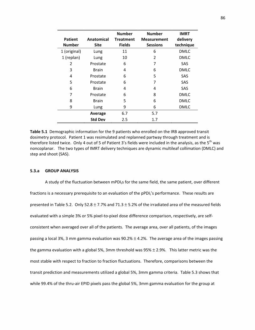
86

Patient Number

Anatomical Site

Number Treatment

Fields

Number Measurement

Sessions

IMRT delivery

technique 1 (original) Lung 11 6 DMLC 1 (replan) Lung 10 2 DMLC

2 Prostate 6 7 SAS 3 Brain 4 6 DMLC 4 Prostate 6 5 SAS 5 Prostate 6 7 SAS 6 Brain 4 4 SAS 7 Prostate 6 8 DMLC 8 Brain 5 6 DMLC 9 Lung 9 6 DMLC

Average 6.7 5.7 Std Dev 2.5 1.7

Table 5.1 Demographic information for the 9 patients who enrolled on the IRB approved transit dosimetry protocol. Patient 1 was resimulated and replanned partway through treatment and is therefore listed twice. Only 4 out of 5 of Patient 3’s fields were included in the analysis, as the 5th was noncoplanar. The two types of IMRT delivery techniques are dynamic multileaf collimation (DMLC) and step and shoot (SAS).

5.3.a GROUP ANALYSIS

A study of the fluctuation between mPDIts for the same field, the same patient, over different

fractions is a necessary prerequisite to an evaluation of the pPDIt’s performance. These results are

presented in Table 5.2. Only 52.8 ± 7.7% and 71.3 ± 5.2% of the irradiated area of the measured fields

evaluated with a simple 3% or 5% pixel-to-pixel dose difference comparison, respectively, are self-

consistent when averaged over all of the patients. The average area, over all patients, of the images

passing a local 3%, 3 mm gamma evaluation was 90.2% ± 4.2%. The average area of the images passing

the gamma evaluation with a global 5%, 3mm threshold was 95% ± 2.9%. This latter metric was the

most stable with respect to fraction to fraction fluctuations. Therefore, comparisons between the

transit prediction and measurements utilized a global 5%, 3mm gamma criteria. Table 5.3 shows that

while 99.4% of the thru-air EPID pixels pass the global 5%, 3mm gamma evaluation for the group at

87

large, 89.1% pass under transit conditions. The transit comparisons also had a larger spread in results as

indicated by the larger standard deviation.

Patient number

Average Area < +/- 3%

difference

Average Area < +/- 5%

difference

Average Area local 3%/3mm

γ < 1

Average Area global 5%/3 mm

γ < 1 2 57.4 74.7 90.9 95.5 3 59.9 72.9 85.7 90.1 4 49.0 68.3 88.4 94.2 5 46.5 68.1 91.3 96.1 6 49.5 72.0 91.8 97.3 7 48.0 69.0 89.6 94.0 8 67.0 81.4 98.7 99.8 9 45.3 64.4 85.5 92.9

Max 67.0 81.4 98.7 99.8 Min 45.3 64.4 85.5 90.1

Average 52.8 71.3 90.2 95.0 Std Dev 7.7 5.2 4.2 2.9

Table 5.2 Measured transit portal dose images (mPDIts) for the same field over each acquired session were compared using simple percent dose differences (3% and 5%) and gamma analyses (local 3%, 3mm and global 5%, 3mm). These comparisons were then averaged over all of the fields within a patient and presented above. The statistics for the entire group of patients is presented in the bottom half of the table. They indicate that a global 5%, 3mm gamma comparison is a metric that demonstrates stability in the presence of interfraction fluctuations.

88

Result Type

Patient Category

Patient Numbers

Number of Meas

Meas Type

Area global 5%, 3mm γ < 1

max min average std dev p-value

All All 2 - 9 288 Pre-Txt 100 96.1 99.4 1.3 0.026

Transit 99 71.1 89.1 9.8

Site Specific

Prostate 2,4,5,7 163 Pre-Txt 100 99.8 99.9 0.1 0.059

Transit 95.3 83.5 91.7 5.5 Brain 3,6,8 71 Pre-Txt 100 96.1 98.5 2.1

0.408 Transit 99 71.1 88.7 15.3

Lung 9 54 Pre-Txt 99.9 99.9 99.9 - -

Transit 80 80 80 -

Technique Specific

SAS 2,4,5,6 131 Pre-Txt 100 96.1 99 1.9 0.142

Transit 95.9 83.5 92.1 5.9 DMLC 3,7,8,9 157 Pre-Txt 100 99.5 99.8 0.2

0.124 Transit 99 71.1 86.1 12.8

Table 5.3 Summary of EPID dosimetry results for the entire patient group as well as anatomical subgroups and delivery techniques. Pre-treatment and transit gamma comparisons between the respective measured and predicted images are presented for each grouping. The results were averaged over each patient. The maximum and minimum columns in the table refer to the patient in each subgroup with the highest or lowest average area passing the gamma criteria. The column labeled “average” refers to the average of the individual patient averages. The max, min, and average values reported in the lung subgroup were all the same because there was only one patient. A student’s t-test was used to report the significance between the differences in the pre-treatment and transit results. Only trends could be identified due to the small number of patients in this study.

89

Figure 5.1 Representative (global 5%, 3 mm) gamma analysis images for prostate, brain, and lung patients. The analysis was carried out between measured and predicted transit portal dose images. The sharp edge in the stripe of failing pixels in the brain field in the second row indicates that part of the patient support assembly may be interfering with the transit measurement.

Number of

patients Number of

measurements

Average Area global 5%/3 mm

γ < 1 1 Standard Deviation

All patients & fields 8 288 89.1% 9.8 %

Subset: Definitely no PSA 6 100 95.7% 2.4 %

Table 5.4 The gamma comparison results for a subset of beams that definitely did not traverse the attenuating components of the patient support assembly (PSA) are presented below the results for all patients and fields. There is approximately a 7% increase in gamma pass rate for this subset over the entire set of analyzed beams.

90

The remainder of Table 5.3 breaks the patients into subgroups based on their specific

anatomical site or IMRT technique. Only trends can only be identified due to the small number of

patients in the study. There is an indication that thoracic treatments may be more difficult to verify than

prostate or brain treatments. The IMRT delivery technique, SAS or DMLC, does not appear to have an

appreciable effect on the transit dosimetry results. Figure 5.1 displays typical gamma images by site.

Some fields, such as the brain field shown in the second row of Figure 5.1, were noted to match well

except for distinct stripes of falling pixels. These stripes are due to beam traversal through aspects of

the PSA or immobilization device that was not accounted for in the pPDIt. The subset of fields where

there was no possibility of interference from the PSA was analyzed and the results are presented in

Table 5.4. There is a marked improvement in the gamma pass rate when the PSA does not interfere

with the beam.

5.3.b LUNG PATIENT CASE STUDY

A transit dosimetry algorithm with sufficient specificity would be expected to flag patients with

a deformation in the internal anatomy. Patient 1 in Table 5.1 was a lung patient whose course of

treatment was complicated by large internal changes. Figure 5.2 presents transverse CT slices from the

patient’s original planning CT scan. Bilateral pleural effusion can be appreciated in the posterior aspect

of the lungs as well as in the anterior aspect of the left lung. There was approximately 680 cm3 of fluid

between the posterior aspect of the lungs and the chest wall. The patient was planned and treatment

commenced in accordance with his schedule for concomitant chemotherapy. As per departmental

standards, pretreatment through-air EPID IMRT QA was performed. Transit images were acquired

during the first treatment fraction. The results from both measurements are shown in Table 5.5. The

pretreatment results indicated that the plan was correctly transferred to the treatment machine.

However, as shown in Figure 5.3, the mPDIts matched very poorly with the pPDIts. On average, only 65%

of the area of the mPDIts passed a global 5%, 3mm gamma evaluation.

91

The physician opted to perform a cone beam CT (CBCT) of the patient in the treatment position

before the delivery of the next fraction. Slices from the CBCT are displayed in Figure 5.2. The posterior

fluid had been resolved between the time of simulation and treatment delivery. The EPID transit

dosimetry had correctly identified that the treatment conditions were not consistent with the simulated

conditions. Therefore, the patient was resimulated and replanned. Treatment with the original plan

continued while the new plan was constructed. When the new plan was ready for treatment, it was

verified through-air, and then applied to the patient. The results of the new transit measurements are

shown in Table 5.5 and Figure 5.3. On average, the area passing a global 5%, 3mm gamma criteria for

the resimulated plan is similar to the results shown for the 8 patients in the group analysis.

Figure 5.2 Computed tomography (CT) images for Patient 1 from Table 5.1. Corresponding slices from the original planning CT, a conebeam CT (CBCT) acquired on the linear accelerator immediately before a treatment session, and the resimulation planning CT are displayed in the first, second, and third columns respectively. The gross tumor volume (GTV) is delineated in cyan and the planning target volume (PTV) is drawn in green. The fluid in the posterior aspect of the bilateral lungs (red arrows) seen in the first column is clearly resolved in the second and third columns.

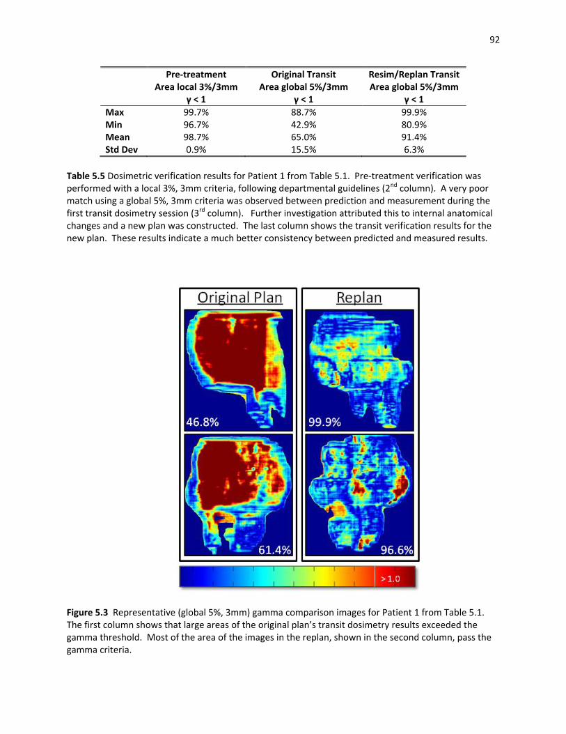
92

Pre-treatment Area local 3%/3mm

γ < 1

Original Transit Area global 5%/3mm

γ < 1

Resim/Replan Transit Area global 5%/3mm

γ < 1 Max 99.7% 88.7% 99.9% Min 96.7% 42.9% 80.9% Mean 98.7% 65.0% 91.4% Std Dev 0.9% 15.5% 6.3%

Table 5.5 Dosimetric verification results for Patient 1 from Table 5.1. Pre-treatment verification was performed with a local 3%, 3mm criteria, following departmental guidelines (2nd column). A very poor match using a global 5%, 3mm criteria was observed between prediction and measurement during the first transit dosimetry session (3rd column). Further investigation attributed this to internal anatomical changes and a new plan was constructed. The last column shows the transit verification results for the new plan. These results indicate a much better consistency between predicted and measured results.

Figure 5.3 Representative (global 5%, 3mm) gamma comparison images for Patient 1 from Table 5.1. The first column shows that large areas of the original plan’s transit dosimetry results exceeded the gamma threshold. Most of the area of the images in the replan, shown in the second column, pass the gamma criteria.

93

5.4 DISCUSSION

One purpose of this feasibility study was to identify challenges that may arise in the course of a

widespread clinical adoption of EPID transit dosimetry. One geometric challenge is that 2 out of 11

(18%) patients were rejected from the protocol because the majority of their planned fields had

combinations of couch and gantry angle that would cause the EPID to collide with the patient or the

PSA. Another known geometric issue is that the maximum deliverable field size is larger than the

maximum verifiable field size due to the 30 x 40 cm2 physical size of the detector. These physical

limitations prevent EPID transit dosimetry from being applied to the entire patient population.

Alternate verification methods would have to be developed and utilized if verification during treatment

is desired for these subgroups.

Patient immobilization devices and the PSA can also be problematic. If they obstruct the beam’s

entrance into the patient, attenuation corrections must be made in order to deliver the correct dose to

the target. If these devices are distal of the patient, no corrections should be made. The target dose

would be correct but the EPID would measure a lower dose than predicted. Many immobilization

devices are low density and are often attributed a negligible attenuation factor. However, the Varian

Exact Couch PSA used in this study has been shown to have an angle dependent attenuation factor that

can be as large as 26.8%29. The support bars of the PSA can be manually shifted along the bottom of the

couch in order to prevent a beam from traversing them. The linac’s light field makes this relatively

simple on the entrance side of the patient, but there is no such guide to help position the bars on the

exit side.

Manual sliding of the bars increases patient treatment time because the therapists have to

enter and leave the vault between fields. In the compilation of the data in Table 5.3, no special effort

was made to slide the bars out of the beam path on the exit side of the Exact couch. However, Table 5.4

indicates that the transit verification results would be improved if the PSA was either accounted for in

94

the pPDIt or was moved out of the path of the beam. In order to improve the verification results, but

not increase the treatment time, it may be useful in future applications to model the PSA in the PDIt

prediction.

Newer versions of the Eclipse TPS software include the ability to model the PSA bars as part of

the treatment plan. Ali, et al., have shown that there is a substantial improvement in agreement

between their pPDIts and mPDIts after their PSA model was applied. The mean dose difference between

predictions and measurements decreased from 5.5% to less than 1% for a 6 MV beam through a lung

phantom. Similarly, the area failing a local 3%, 3 mm gamma criteria decreased from a range of 25.6 %

to 52.1% to a range of 0.2% to 3.6%. The authors caution, however, that some care must be taken to

ensure that the couch position in the model is consistent with the true couch position30. An

inconsistency will lead to a worse outcome than making no correction at all31. Since the position of the

Exact couch bars are not electronically detected by the machine, or recorded in the RNV system, the

onus would remain on the therapy staff in the treatment room to manually ensure that they are in the

modeled position.

The inconvenience of the positioning of the PSA bars is compounded for transit dosimetry by the

need to also correctly position the EPID. As in our previous publication16, a 35 cm air gap between the

exit surface of the patient and the detector layer was utilized. This typically results in a different SDD for

each planned gantry angle. Although the EPID can be automatically moved to the preprogrammed

position from outside of the vault, only 323 out of the 357 mPDIs (90.48%) in this study were acquired at

the correct SDD. The pPDIt and mPDIt do not match if acquired at different SDDs due to divergence and

the inverse square law. The number of incorrect SDDs would be expected to lessen once the therapists

were more familiar with the process. However, a software interlock which stops treatment from

commencing if the EPID is improperly positioned would be necessary for routine, commercial, EPID

transit dosimetry. One area for future investigation may be a generalization of the 2DTD prediction

95

algorithm such that a large, but constant, SDD may be used for all fields within a patient’s plan. While it

would still be possible to treat with the wrong SDD, the therapists would only have to remember to

place the imager correctly once per patient rather than once per beam.

The IAS3 software stops accumulation of the mPDIt signal if the delivery is stopped mid-field.

This may occur as a result of a linac interlock or by manual therapist intervention for any number of

reasons, such as a patient signaling for help. There were a few instances for patients on this protocol

where the beam was stopped because it was realized that the EPID SDD was incorrect. Any subsequent

EPID dose from the completion of the beam’s delivery is not recorded. Therefore, even if the patient

ultimately receives the correct dose, the comparison between a partial mPDIt and the pPDIt would show

a failure. The effect of beam holds due to MLC leaf motion or respiratory gating on the mPDIts was not

investigated in this study, but could be areas of interest for the future.

The clinical workflow for EPID transit dosimetry in our implementation differs from some

methods presented in the literature. Our approach utilizes pretreatment EPID dosimetry with a

stringent local 3%, 3mm gamma criteria to prevent technical sources of systematic error. Then, transit

dosimetry is used throughout the treatment course to ensure that there are no systematic errors caused

either by patient anatomy and positioning or technical errors that occurred after the pretreatment

checks. A global 5%, 3 mm gamma was chosen as the evaluation metric in the transit setting as a result

of our interfraction mPDIt analysis. Use of a more stringent evaluation criterion could frequently and

unnecessarily interrupt a patient’s treatment while an investigation is carried out to find the source of

the small errors. These errors are likely due to transient internal changes such as organ filling or gas14, 15,

32, 33.

A group at the Netherlands Cancer Institute has implemented an alternate paradigm where

fractionated treatments are not routinely verified with measurements before treatment1. Instead, in

vivo PDIs for a number of fractions are combined and evaluated using a global 3%, 3mm gamma criteria.

96

Combining the fractions separates random from systematic errors. Their technique significantly reduces

the time spent performing patient specific QA15. However, this is at the cost of potentially exposing the

patient to errors over those first few fractions that could have been caught with a pre-treatment

measurement.

The 2DTD’s ability to identify treatment related errors is illustrated in the case study. Patient 1

would have been treated throughout his entire course with the original plan had he not been enrolled

on the protocol. This would have resulted in higher than planned doses to the target and critical organs.

External changes, such as weight gain or loss, may be noted by therapists and prompt an investigation

into whether or not the plan is still applicable. Internal changes, such as the accumulation or clearing of

fluid in the lungs, cannot be identified by a therapist’s visual inspection. This is why many modern linacs

have image guidance capabilities such as planar kV radiographs or CBCT. However logistical reasons,

such as patient throughput and treatment time, may limit the use of these techniques for conventionally

fractionated patients. In a recently published survey, 62% of physician respondents said that they used

IGRT rarely (< 25% of their patients) or infrequently (between 25-50% of their patients)34. Another

possible consideration is that daily CBCT applied over the course of a conventionally fractioned

treatment could deliver doses of tens, even hundreds, of centigray to superficial organs such as skin,

thyroid, lens of the eye, and external genitalia35-37.

Two dimensional transit dosimetry is advantageous in that it identifies whether a treatment is

delivered properly without additional dose and with a negligible increase in time. The only extra time

necessary during treatment is the moment it takes to extend the EPID to the predefined position behind

the patient. While analysis was performed off-line in this feasibility study, the ultimate goal would be

to perform real time monitoring with automated analysis. Interaction with the user would only be

necessary if the results were outside of a defined tolerance. This should catch the most severe errors,

such as those presented in the popular press38, before they do irrevocable harm to the patient.

97

The weakness in 2D transit dosimetry is that no anatomical information accompanies a reported

discrepancy between the mPDIt and the pPDIt. This makes it is difficult to come to an informed clinical

decision about how to proceed. Therefore, cases that exceed a set tolerance in 2DTD could be referred

for further investigation. This may take the form of more advanced imaging techniques, such as CBCT,

or could include more advanced dosimetric techniques such as 3D EPID dosimetry. In the latter

approach, the primary fluence is extracted from the measured transit dose and backprojected through

the planning CT or a CBCT for the purposes of a volumetric dose calculation. A DVH can be constructed

in order to fully compare the delivered versus planned doses to the patient11, 39. This method is

intensive both in terms of computation time and in the human time spent evaluating the plan.

However, application of a two step approach, where the entire patient population is quickly and

quantifiably screened with 2DTD and then fields that are flagged as out of tolerance are more

thoroughly investigated, would ensure that the time resources devoted to 3D dosimetry would be well

spent.

5.5 CONCLUSION

The 2DTD algorithm, previously described and verified in a phantom study16, is feasible for use

in treatment delivery verification for real patients. On average, 89.1% of the pixels in the mPDIts pass a

gamma comparison with the corresponding pPDIts using a global 5%, 3mm criteria. A clinical case study

featuring a patient who had bilateral pleural effusion during simulation and planning that had resolved

by treatment time was used to illustrate the important role that 2D EPID transit dosimetry can play in

indicating whether a treatment delivery is inconsistent with the original plan.

Future areas of research and investigation will be focused on improving the gamma comparison

results through the incorporation of PSA modeling in the creation of the pPDIt. Clinical workflow

improvements can also be achieved by modifying the 2DTD algorithm to generalize the 35 cm exit

surface to detector air gap. The ultimate goal is to perform transit dosimetry in real time so that grave

98

errors can be identified and stopped as they are occurring. 2D transit dosimetry is a worthwhile

treatment verification technique that strikes a balance between usefulness and efficiency.

99

BIBLIOGRAPHY

1. A. Mans, M. Wendling, L. N. McDermott, J. J. Sonke, R. Tielenburg, R. Vijlbrief, B. Mijnheer, M. van Herk and J. C. Stroom, "Catching errors with in vivo EPID dosimetry," Med Phys 37, 2638-2644 (2010).

2. B. Mijnheer, A. Mans, I. Olaciregui-Ruiz, J.-J. Sonke, R. Tielenburg, M. V. Herk, R. Vijlbrief and J.

Stroom, "2D AND 3D dose verification at The Netherlands Cancer Institute Antoni van Leeuwenhoek Hospital using EPIDs," Journal of Physics: Conference Series 250, 012020 (2010).

3. B. Mijnheer, "State of the art of in vivo dosimetry," Radiat Prot Dosimetry 131, 117-122 (2008). 4. A. Van Esch, T. Depuydt and D. P. Huyskens, "The use of an aSi-based EPID for routine absolute

dosimetric pre-treatment verification of dynamic IMRT fields," Radiother Oncol 71, 223-234 (2004).

5. W. van Elmpt, L. McDermott, S. Nijsten, M. Wendling, P. Lambin and B. Mijnheer, "A literature

review of electronic portal imaging for radiotherapy dosimetry," Radiother Oncol 88, 289-309 (2008).

6. B. Warkentin, S. Steciw, S. Rathee and B. G. Fallone, "Dosimetric IMRT verification with a flat-

panel EPID," Med Phys 30, 3143-3155 (2003). 7. P. Winkler and D. Georg, "An intercomparison of 11 amorphous silicon EPIDs of the same type:

implications for portal dosimetry," Phys Med Biol 51, 4189-4200 (2006). 8. P. Winkler, A. Hefner and D. Georg, "Dose-response characteristics of an amorphous silicon

EPID," Med Phys 32, 3095-3105 (2005). 9. S. M. Nijsten, B. J. Mijnheer, A. L. Dekker, P. Lambin and A. W. Minken, "Routine individualised

patient dosimetry using electronic portal imaging devices," Radiother Oncol 83, 65-75 (2007). 10. K. L. Pasma, M. Kroonwijk, S. Quint, A. G. Visser and B. J. Heijmen, "Transit dosimetry with an

electronic portal imaging device (EPID) for 115 prostate cancer patients," Int J Radiat Oncol Biol Phys 45, 1297-1303 (1999).

11. W. van Elmpt, S. Nijsten, S. Petit, B. Mijnheer, P. Lambin and A. Dekker, "3D in vivo dosimetry

using megavoltage cone-beam CT and EPID dosimetry," Int J Radiat Oncol Biol Phys 73, 1580-1587 (2009).

12. M. van Zijtveld, M. Dirkx, M. Breuers, H. de Boer and B. Heijmen, "Portal dose image prediction

for in vivo treatment verification completely based on EPID measurements," Med Phys 36, 946-952 (2009).

13. R. Pecharroman-Gallego, A. Mans, J. J. Sonke, J. C. Stroom, I. Olaciregui-Ruiz, M. van Herk and B.

J. Mijnheer, "Simplifying EPID dosimetry for IMRT treatment verification," Med Phys 38, 983-992.

100

14. L. N. McDermott, M. Wendling, J. Nijkamp, A. Mans, J. J. Sonke, B. J. Mijnheer and M. van Herk, "3D in vivo dose verification of entire hypo-fractionated IMRT treatments using an EPID and cone-beam CT," Radiother Oncol 86, 35-42 (2008).

15. L. N. McDermott, M. Wendling, J. J. Sonke, M. van Herk and B. J. Mijnheer, "Replacing

pretreatment verification with in vivo EPID dosimetry for prostate IMRT," Int J Radiat Oncol Biol Phys 67, 1568-1577 (2007).

16. S. L. Berry, R.D. Sheu, C. S. Polvorosa and C.S. Wuu, "Implementation of EPID transit dosimetry

based on a through-air dosimetry algorithm," Medical Physics 39, 87-98 (2012). 17. J. J. Sonke and J. Belderbos, "Adaptive radiotherapy for lung cancer," Semin Radiat Oncol 20, 94-

106 (2010). 18. J. L. Barker, Jr., A. S. Garden, K. K. Ang, J. C. O'Daniel, H. Wang, L. E. Court, W. H. Morrison, D. I.

Rosenthal, K. S. Chao, S. L. Tucker, R. Mohan and L. Dong, "Quantification of volumetric and geometric changes occurring during fractionated radiotherapy for head-and-neck cancer using an integrated CT/linear accelerator system," Int J Radiat Oncol Biol Phys 59, 960-970 (2004).

19. Y. C. Kuo, T. H. Wu, T. S. Chung, K. W. Huang, K. S. Chao, W. C. Su and J. F. Chiou, "Effect of

regression of enlarged neck lymph nodes on radiation doses received by parotid glands during intensity-modulated radiotherapy for head and neck cancer," Am J Clin Oncol 29, 600-605 (2006).

20. C. Lee, K. M. Langen, W. Lu, J. Haimerl, E. Schnarr, K. J. Ruchala, G. H. Olivera, S. L. Meeks, P. A.

Kupelian, T. D. Shellenberger and R. R. Manon, "Assessment of parotid gland dose changes during head and neck cancer radiotherapy using daily megavoltage computed tomography and deformable image registration," Int J Radiat Oncol Biol Phys 71, 1563-1571 (2008).

21. Varian-Medical-Systems, "Eclipse Algorithms Reference Guide ", Vol. B500298R01A, (Finland,

2006), pp. 7-1 - 7-28. 22. S. L. Berry, C. S. Polvorosa and C. S. Wuu, "A field size specific backscatter correction algorithm

for accurate EPID dosimetry," Med Phys 37, 2425-2434 (2010). 23. C. Yeboah and S. Pistorius, "Monte Carlo studies of the exit photon spectra and dose to a

metal/phosphor portal imaging screen," Med Phys 27, 330-339 (2000). 24. R. Boellaard, M. van Herk and B. J. Mijnheer, "A convolution model to convert transmission dose

images to exit dose distributions," Med Phys 24, 189-199 (1997). 25. W. Swindell and P. M. Evans, "Scattered radiation in portal images: a Monte Carlo simulation

and a simple physical model," Med Phys 23, 63-73 (1996). 26. D. A. Low, W. B. Harms, S. Mutic and J. A. Purdy, "A technique for the quantitative evaluation of

dose distributions," Med Phys 25, 656-661 (1998).

101

27. B. Mijnheer and D. Georg, "Guidelines for the Verification of IMRT," in ESTRO Physics Booklets, Vol. 9, edited by ESTRO (ESTRO, Brussels, 2008), pp. 136.

28. J. Van Dyk, R. B. Barnett, J. E. Cygler and P. C. Shragge, "Commissioning and quality assurance of

treatment planning computers," Int J Radiat Oncol Biol Phys 26, 261-273 (1993). 29. H. Li, A. K. Lee, J. L. Johnson, R. X. Zhu and R. J. Kudchadker, "Characterization of dose impact on

IMRT and VMAT from couch attenuation for two Varian couches," J Appl Clin Med Phys 12, 3471 (2011).

30. A. S. Ali, M. L. Dirkx, M. G. Breuers and B. J. Heijmen, "Inclusion of the treatment couch in portal

dose image prediction for high precision EPID dosimetry," Med Phys 38, 377-381 (2011). 31. K. B. Pulliam, R. M. Howell, D. Followill, D. Luo, R. A. White and S. F. Kry, "The clinical impact of

the couch top and rails on IMRT and arc therapy," Phys Med Biol 56, 7435-7447 (2011). 32. M. Kroonwijk, K. L. Pasma, S. Quint, P. C. Koper, A. G. Visser and B. J. Heijmen, "In vivo dosimetry

for prostate cancer patients using an electronic portal imaging device (EPID); demonstration of internal organ motion," Radiother Oncol 49, 125-132 (1998).

33. R. Boellaard, M. van Herk, H. Uiterwaal and B. Mijnheer, "First clinical tests using a liquid-filled

electronic portal imaging device and a convolution model for the verification of the midplane dose," Radiother Oncol 47, 303-312 (1998).

34. D. R. Simpson, J. D. Lawson, S. K. Nath, B. S. Rose, A. J. Mundt and L. K. Mell, "A survey of image-

guided radiation therapy use in the United States," Cancer 116, 3953-3960. 35. M. W. Kan, L. H. Leung, W. Wong and N. Lam, "Radiation dose from cone beam computed

tomography for image-guided radiation therapy," Int J Radiat Oncol Biol Phys 70, 272-279 (2008).

36. D. E. Hyer, C. F. Serago, S. Kim, J. G. Li and D. E. Hintenlang, "An organ and effective dose study

of XVI and OBI cone-beam CT systems," J Appl Clin Med Phys 11, 3183 (2010). 37. G. X. Ding and C. W. Coffey, "Radiation dose from kilovoltage cone beam computed tomography

in an image-guided radiotherapy procedure," Int J Radiat Oncol Biol Phys 73, 610-617 (2009). 38. W. Bogdanich, "A Lifesaving Tool Turned Deadly," in The New York Times, (New York, Jan 24,

2010), pp. A1. 39. W. van Elmpt, S. Nijsten, B. Mijnheer, A. Dekker and P. Lambin, "The next step in patient-specific

QA: 3D dose verification of conformal and intensity-modulated RT based on EPID dosimetry and Monte Carlo dose calculations," Radiother Oncol 86, 86-92 (2008).

102

Chapter 6

Summary and Conclusion

103

6.1. SUMMARY AND CONCLUSION

Designed for imaging, amorphous silicon (aSi) electronic portal imaging devices (EPIDs) are also

useful for dosimetric applications. Their high resolution and integration with the medical linear

accelerator (linac) represent advantages over other planar dosimeters1, 2. All EPID data is digital, unlike

film, so there is no need for processing and scanning3. Despite these benefits, the EPID is underutilized

for dosimetry. This may be due to design features that are helpful or innocuous for imaging applications

but become problematic for dosimetry. We have offered solutions for a number of these problems.

First, the support arm that attaches the EPID to the linac introduces backscattered x-rays into

the EPID photodiode array. This causes pixel values in the measured portal dose images (mPDIs) to be

misreported. How much of this arm gets irradiated depends upon the field size and EPID position. The

error in the pixel reading is related to the difference between the amount of backscatter present at the

time of the flood field (FF) calibration and that of subsequent treatment field irradiations. Errors of 5%

to 6.5% have been observed4, 5. Some investigators have added shielding to the EPID to absorb these

backscattered x-rays6. This could affect the detector’s mechanical stability. We introduced a field size

specific backscatter correction algorithm in Chapter 2 that corrects mPDIs for this erroneous signal

without modifications of the hardware. Statistically significant improvements in the dosimetric

comparisons between predicted portal dose images (pPDIs) and mPDIs were achieved once the

backscatter algorithm was applied.

The experiment carried out in Chapter 3 was designed to verify that the equipment used for this

research project was sufficiently free from positional uncertainty and gravitational sag. Transit

dosimetry must provide correct information about both the magnitude and location of the dose

distribution. To achieve the latter, users with older hardware models have either employed additional

equipment to stabilize the EPID or had to frequently reposition the detector7. Neither of these solutions

is reasonable for widespread clinical implementation which prioritizes increased patient throughput and

104

reduced treatment times. A modern set of hardware, the aS1000 EPID attached to a Varian TrilogyTx

linac with an Exact Arm (E-arm) (Varian Medical Systems, Palo Alto, CA), was shown to have a positional

accuracy within 1 mm. This is adequate for transit dosimetry.

A major impediment to aSi EPID transit dosimetry is the high atomic number (Z) of its

component parts. These materials were originally chosen so that the EPID can produce radiographic

images with little dose3. However, this causes the EPID to act as a non-tissue equivalent dosimeter. It is

sensitive to the quality of the incident photon spectrum8, 9. The relationship of EPID pixel value to dose

has a complex dependence on the irradiated field size, the EPID pixel location, and the amount of

attenuation and scatter arising from the patient or phantom. The 2D transit dosimetry (2DTD)

algorithm, a model to describe this relationship, was proposed in Chapter 4. The algorithm’s

performance was verified through phantoms of varying complexity.

Upon demonstrating the efficacy of the algorithm on phantom materials, permission to proceed

with an experiment on human subjects was solicited from, and granted by, Columbia University’s

Institutional Review Board (IRB). The methodology and results are presented in Chapter 5. The

feasibility of using transit dosimetry to verify the radiation dose delivered to patients was confirmed. A

case study was presented which described an instance where EPID transit dosimetry identified an

erroneous dose delivery. The error was caused by a change in the patient’s internal anatomy some time

after the acquisition of the planning scan. It was unlikely to have been caught by any other means since

the setup verification was planned to only include planar localization radiographs, not volumetric

imaging.

The formulations of the backscatter and 2DTD algorithms represent considerable progress

towards the improvement of EPID dosimetry. The backscatter correction algorithm will improve both

pretreatment intensity modulated radiotherapy (IMRT) quality assurance (QA) and transit dosimetry.

EPID pretreatment IMRT QA already has an established user base that could benefit from the

105

backscatter correction. Until recently, transit dosimetry has been generally constrained to large

research medical centers10-13. The decision to base our 2DTD algorithm on top of the commercially

available Van Esch algorithm14 could help to accelerate the expansion of this essential dosimetric

procedure to more treatment centers.

106

BIBLIOGRAPHY

1. D. Letourneau, M. Gulam, D. Yan, M. Oldham and J. W. Wong, "Evaluation of a 2D diode array for IMRT quality assurance," Radiother Oncol 70, 199-206 (2004).

2. J. Herzen, M. Todorovic, F. Cremers, V. Platz, D. Albers, A. Bartels and R. Schmidt, "Dosimetric

evaluation of a 2D pixel ionization chamber for implementation in clinical routine," Phys Med Biol 52, 1197-1208 (2007).

3. L. E. Antonuk, "Electronic portal imaging devices: a review and historical perspective of

contemporary technologies and research," Phys Med Biol 47, R31-65 (2002). 4. P. B. Greer, P. Cadman, C. Lee and K. Bzdusek, "An energy fluence-convolution model for

amorphous silicon EPID dose prediction," Med Phys 36, 547-555 (2009). 5. L. Ko, J. O. Kim and J. V. Siebers, "Investigation of the optimal backscatter for an aSi electronic

portal imaging device," Phys Med Biol 49, 1723-1738 (2004). 6. J. A. Moore and J. V. Siebers, "Verification of the optimal backscatter for an aSi electronic portal

imaging device," Phys Med Biol 50, 2341-2350 (2005). 7. M. W. Grattan and C. K. McGarry, "Mechanical characterization of the varian Exact-arm and R-

arm support systems for eight aS500 electronic portal imaging devices," Med Phys 37, 1707-1713 (2010).

8. C. Kirkby and R. Sloboda, "Consequences of the spectral response of an a-Si EPID and

implications for dosimetric calibration," Med Phys 32, 2649-2658 (2005). 9. C. Yeboah and S. Pistorius, "Monte Carlo studies of the exit photon spectra and dose to a

metal/phosphor portal imaging screen," Med Phys 27, 330-339 (2000). 10. W. van Elmpt, L. McDermott, S. Nijsten, M. Wendling, P. Lambin and B. Mijnheer, "A literature

review of electronic portal imaging for radiotherapy dosimetry," Radiother Oncol 88, 289-309 (2008).

11. L. N. McDermott, M. Wendling, J. Nijkamp, A. Mans, J. J. Sonke, B. J. Mijnheer and M. van Herk,

"3D in vivo dose verification of entire hypo-fractionated IMRT treatments using an EPID and cone-beam CT," Radiother Oncol 86, 35-42 (2008).

12. L. N. McDermott, M. Wendling, J. J. Sonke, M. van Herk and B. J. Mijnheer, "Replacing

pretreatment verification with in vivo EPID dosimetry for prostate IMRT," Int J Radiat Oncol Biol Phys 67, 1568-1577 (2007).

13. S. M. Nijsten, W. J. van Elmpt, M. Jacobs, B. J. Mijnheer, A. L. Dekker, P. Lambin and A. W.

Minken, "A global calibration model for a-Si EPIDs used for transit dosimetry," Med Phys 34, 3872-3884 (2007).

107

14. A. Van Esch, T. Depuydt and D. P. Huyskens, "The use of an aSi-based EPID for routine absolute dosimetric pre-treatment verification of dynamic IMRT fields," Radiother Oncol 71, 223-234 (2004).

108

Chapter 7

Suggestions for Future Study

109

7.1. SUGGESTIONS FOR FUTURE STUDY

While aSi EPID dosimetry has been an area of study for over a decade1-5, widespread clinical use

has not been achieved. However, there are a number of independent developments in the field of

radiation oncology that indicate that EPID dosimetry could take a larger role in the near future. First,

the prevalence of megavoltage (MV) EPID imaging in patient localization has diminished. Technologies

such as gantry and room mounted kilovoltage (kV) x-ray tubes and detectors have become widespread6.

The dominance of the photoelectric effect in kV x-rays allows for clear differentiation between bone,

muscle, and air, making these devices superior for patient setup verification. As this trend continues,

manufacturers may have more incentive to engineer MV EPIDs for dosimetric applications.

Second, the growth of the volumetric modulated arc therapy (VMAT) technique7 has led to a

class of linacs engineered to have great precision in the presence of gravitational forces and mechanical

stress. VMAT is a treatment delivery method where the beam remains on as the gantry and MLC move

continuously. The necessary linac stability with gantry rotation translates to improvements in EPID

positional accuracy, as demonstrated in Chapter 3. This in turn allows for more accurate transit

dosimetry.

Third, there is growing consensus in the community that most planar IMRT QA detectors, for

example diode and ionization chamber arrays, do not have a sufficient data density to produce

meaningful results8, 9. With a pixel size of 0.39 mm and a detection area of 30 x 40 cm2, the EPID has

been shown to be an excellent high resolution alternative10.

Finally, regulatory demands to routinely verify patient treatment delivery with in vivo dose

measurements have been increasing. In vivo dosimetry is now mandatory in countries such as France,

Denmark, and Sweden11. While point detectors have historically been utilized for this task, verification

at a single point does not describe the complex modulation in a modern treatment delivery12. This

110

complexity can result in undetected catastrophic treatment errors, such as those recently reported in

the popular press13-15. Two dimensional detectors are necessary.

Based on these emerging trends, continued research and development in EPID dosimetry is

justifiable. The implementation of EPID dosimetry in the clinic is one area that needs attention. An

appropriate balance between the time spent performing dosimetric validation and efficiency in planning

and treatment needs to be developed. How often should transit dosimetry be applied during a patient’s

course of treatment? How quickly do the acquired mPDIs need to be analyzed by a physicist

(immediately, within a day, within a week)? Are there subpopulations of patients that would benefit

more or less? Are there particular treatment sites that would benefit more or less? Is pretreatment

IMRT QA necessary if transit dosimetry is routinely performed? The Netherlands Cancer Institute has

abandoned routine pretreatment IMRT QA in favor of in vivo EPID measurements acquired over the first

few fractions16. Is this safe?

There are also a number of questions about how to best analyze the mPDIs. Which evaluation

metrics correlate with deliveries that are substantially different from the original plan9? Should each

mPDI be analyzed in isolation or should it be reviewed as one instance out of a series of periodic

acquisitions of that field? The latter would help to differentiate between random and systematic

errors16. Both of these questions are related to the detector’s sensitivity and specificity. Further studies

should be carried out in order to determine the lower limit at which the EPID is able to detect a change.

For example, what is the minimum difference in patient thickness or minimum error in patient

alignment that would be identified by the EPID? Other areas that could be analyzed may include, but

not be limited to, changes in breathing pattern or errors in leaf sequence delivery. Phantom studies

could be designed where intentional changes of these types are introduced and the performance of the

EPID as a transit dosimeter is characterized.

111

What steps should be taken if a mPDI analysis exceeds a predefined action level? One option,

illustrated in Chapter 5, is to pursue additional imaging. Another option would be to investigate the

delivered dose to the patient using 3D EPID dosimetry techniques. The latter would involve extracting

the primary fluence from the transit PDI. That fluence would then be backprojected through a CT scan

of the patient to reconstruct the delivered dose17, 18. Three dimensional techniques not only report

whether there is a pass or fail, but also how that pass or fail correlates with changes in the patient’s

planned dose distribution. This extra information comes at the expense of a large increase in the

physicist and physician’s time commitment. This cost would be prohibitive if applied to all patients

within a radiation oncology clinic. Therefore, a paradigm where an automated 2D EPID dosimetry

procedure is used as a screening mechanism that can refer troublesome patients for 3D EPID dosimetry

could be useful.

The 2DTD algorithm needs further development in order to transform it from an investigational

tool to a routine clinical tool. First, better integration with the treatment planning system (TPS),

treatment management system (TMS), 2DTD prediction software, and dosimetric analysis software is

necessary. Too many manual imports and exports are currently necessary to move files between these

applications. Manual file transfer is not only inefficient but introduces errors into the radiation therapy

process19. The desired EPID position for each individual field also currently needs to be manually

entered into the TMS. The EPID can subsequently be moved to that preprogrammed location.

However, the treatment delivery software used in this study allows the linac to treat even if the EPID is

retracted or not at the preprogrammed position. As a result, the therapists acquired approximately

9.5% of the transit mPDIs in Chapter 5 at the incorrect source to detector distance (SDD). More robust

control over the EPID positioning would be necessary in a large clinical deployment of transit dosimetry.

Modifications of the current 2DTD prediction algorithm would also have to be made. Methods

to correct for the additional attenuation introduced by the patient support assembly (PSA) were

112

identified in Chapter 5. The PSA’s affect on the delivered patient dose has been an active area of recent

research20-22.

The ultimate goal for 2D EPID dosimetry is online dose monitoring during the patient’s

treatment. The purpose would be to identify a catastrophic treatment related error as it is occurring

and stop it before it is too late. Offline analysis only allows one to make this identification after the fact.

Online analysis requires tight integration between software applications. The analysis software must

work without intervention from the user unless it identifies a field that exceeds a predefined action

level. At that point, the beam delivery should be paused until the user decides how to proceed.

The current 2DTD algorithm creates a prediction based on the delivery of an entire treatment

field. Modifying the algorithm to predict PDIs at some intervals within a given field’s delivery, as would

be necessary for online monitoring, is trivial. The MLC leaf motion files used to define the IMRT delivery

are divided into a finite number of control points. Each one represents a distinct set of MLC positions23.

A subset of these control points can be used as input into the 2DTD algorithm in order to create the

corresponding pPDIs.

Although online patient dose monitoring with the EPID is not yet a reality, much progress has

been made in the improvement and development of EPID dosimetry. It is clear from the large number

of suggestions for further study that EPID dosimetry will remain an area of active and fruitful research

into the future.

113

BIBLIOGRAPHY

1. E. E. Grein, R. Lee and K. Luchka, "An investigation of a new amorphous silicon electronic portal imaging device for transit dosimetry," Med Phys 29, 2262-2268 (2002).

2. B. M. McCurdy, K. Luchka and S. Pistorius, "Dosimetric investigation and portal dose image

prediction using an amorphous silicon electronic portal imaging device," Med Phys 28, 911-924 (2001).

3. L. Parent, J. Seco, P. M. Evans, A. Fielding and D. R. Dance, "Monte Carlo modelling of a-Si EPID

response: the effect of spectral variations with field size and position," Med Phys 33, 4527-4540 (2006).

4. J. V. Siebers, J. O. Kim, L. Ko, P. J. Keall and R. Mohan, "Monte Carlo computation of dosimetric

amorphous silicon electronic portal images," Med Phys 31, 2135-2146 (2004). 5. A. Van Esch, T. Depuydt and D. P. Huyskens, "The use of an aSi-based EPID for routine absolute

dosimetric pre-treatment verification of dynamic IMRT fields," Radiother Oncol 71, 223-234 (2004).

6. D. R. Simpson, J. D. Lawson, S. K. Nath, B. S. Rose, A. J. Mundt and L. K. Mell, "A survey of image-

guided radiation therapy use in the United States," Cancer 116, 3953-3960 (2010). 7. C. X. Yu and G. Tang, "Intensity-modulated arc therapy: principles, technologies and clinical

implementation," Phys Med Biol 56, R31-54 (2011). 8. D. W. Bailey, B. E. Nelms, K. Attwood, L. Kumaraswamy and M. B. Podgorsak, "Statistical

variability and confidence intervals for planar dose QA pass rates," Med Phys 38, 6053-6064 (2011).

9. B. E. Nelms, H. Zhen and W. A. Tome, "Per-beam, planar IMRT QA passing rates do not predict

clinically relevant patient dose errors," Med Phys 38, 1037-1044 (2011). 10. B. E. Nelms, K. H. Rasmussen and W. A. Tome, "Evaluation of a fast method of EPID-based

dosimetry for intensity-modulated radiation therapy," J Appl Clin Med Phys 11, 3185 (2010). 11. D. Ash, "Lessons from Epinal," Clin Oncol (R Coll Radiol) 19, 614-615 (2007). 12. B. Mijnheer, "State of the art of in vivo dosimetry," Radiat Prot Dosimetry 131, 117-122 (2008). 13. W. Bogdanich, "At Hearing on Radiation, Calls for Better Oversight," in The New York Times,

(New York, 2010). 14. W. Bogdanich, "A Lifesaving Tool Turned Deadly," in The New York Times, (New York, Jan 24,

2010), pp. A1. 15. W. Bogdanich, "As Technology Surges, Radiation Safeguards Lag," in The New York Times, (New

York, Jan 27, 2010), pp. A1.

114

16. L. N. McDermott, M. Wendling, J. J. Sonke, M. van Herk and B. J. Mijnheer, "Replacing pretreatment verification with in vivo EPID dosimetry for prostate IMRT," Int J Radiat Oncol Biol Phys 67, 1568-1577 (2007).

17. L. N. McDermott, M. Wendling, J. Nijkamp, A. Mans, J. J. Sonke, B. J. Mijnheer and M. van Herk,

"3D in vivo dose verification of entire hypo-fractionated IMRT treatments using an EPID and cone-beam CT," Radiother Oncol 86, 35-42 (2008).

18. W. van Elmpt, S. Nijsten, S. Petit, B. Mijnheer, P. Lambin and A. Dekker, "3D in vivo dosimetry

using megavoltage cone-beam CT and EPID dosimetry," Int J Radiat Oncol Biol Phys 73, 1580-1587 (2009).

19. G. Leunens, J. Verstraete, W. Van den Bogaert, J. Van Dam, A. Dutreix and E. van der Schueren,

"Human errors in data transfer during the preparation and delivery of radiation treatment affecting the final result: "garbage in, garbage out"," Radiother Oncol 23, 217-222 (1992).

20. H. Li, A. K. Lee, J. L. Johnson, R. X. Zhu and R. J. Kudchadker, "Characterization of dose impact on

IMRT and VMAT from couch attenuation for two Varian couches," J Appl Clin Med Phys 12, 3471 (2011).

21. K. B. Pulliam, R. M. Howell, D. Followill, D. Luo, R. A. White and S. F. Kry, "The clinical impact of

the couch top and rails on IMRT and arc therapy," Phys Med Biol 56, 7435-7447 (2011). 22. J. K. Seppala and J. A. Kulmala, "Increased beam attenuation and surface dose by different couch

inserts of treatment tables used in megavoltage radiotherapy," J Appl Clin Med Phys 12, 3554 (2011).

23. G. J. Budgell, "Temporal resolution requirements for intensity modulated radiation therapy

delivered by multileaf collimators," Phys Med Biol 44, 1581-1596 (1999).

115

GLOSSARY OF ABBREVIATIONS AND ACRONYMS

A

AAPM American Association of Physicists in Medicine

aSi amorphous silicon

ASTRO American Society for Radiation Oncology

C

CAX central axis

CBCT cone beam computed tomography

CIAO complete irradiated area outline

CP central pixel

cPDIe generalized equation corrected portal dose image

cPDIm matrix corrected portal dose image

CS collimator setting

CSF collimator scatter factor

CT computed tomography

CU calibrated units

D

DD dose difference

DDR detector dependent response

DF dark field

DMLC dynamic multileaf collimation

DTA distance to agreement

E

E-arm Exact arm

116

EBRT external beam radiation therapy

EF energy fluence

EPID electronic portal imaging device

ESTRO European Society for Therapeutic Radiology and Oncology

F

FF flood field

4DITC 4D integrated treatment console

FS field size

G

Gd2O2S gadolinium oxysulfide

GTV gross tumor volume

H

HU Hounsfield units

HVL half-value layer

I

IAS3 Image Acquisition System 3 software package

ICRU International Commission on Radiation Units and Measurement

IMRT intensity modulated radiation therapy

IRB institutional review board K

kV kilovoltage

L

linac linear accelerator

LQ linear quadratic

117

M

MC Monte Carlo

MLC multileaf collimator

MOSFET metal oxide field effect transistor

mPDI measured portal dose image

mPDIair through-air measured portal dose image

mPDIt measured transit portal dose image

MRI magnetic resonance imaging

MU monitor unit

MV Megavoltage

N

NIST National Institute of Standards and Technology

O

OAP off-axis pixel

OAR off-axis ratio

OSLD optically stimulated luminescent diode

P

PBDC pencil beam dose calculation

PDI portal dose image

PDIP portal dose image prediction

PET positron emission tomography

pPDI predicted portal dose image

pPDIair through-air predicted portal dose image

pPDIt predicted transit portal dose image

118

pPDItx predicted portal dose image behind a patient or phantom

PSA patient support assembly

PSQA patient specific quality assurance

PTV planning target volume

Q

QA quality assurance

R

RF response function

ROI region of interest

RTP radiation treatment planning

S

SAS step and shoot

SCD source to couch distance

SDD source to detector distance

SF surviving fraction

sPDI symmetric portal dose image

SSD source to surface distance

T

TFT thin-film transistor

TG task group

TLD thermoluminescent diode

TMS treatment management system

TPS treatment planning system

2DkV two-dimensional kilovoltage radiograph

119

2DTD two-dimensional transit dosimetry

V

VMAT volumetric modulated arc therapy

Z

Z atomic number