Embed Size (px)
DESCRIPTION
Unsteady and Steady State
Citation preview
Chapter 3: Heat Conduction
Advanced Heat and Mass Transfer by Amir Faghri, Yuwen Zhang, and John R. Howell
3.3 Unsteady State Heat Conduction
1
� For many applications, it is necessary to consider the
variation of temperature with time.
� In this case, the energy equation for classical heat
conduction, eq. (3.8), should be solved.
� If the thermal conductivity is independent from the
temperature, the energy equation is reduced to eq.
(3.10).
3.3 Unsteady State Heat Conduction3.3 Unsteady State Heat Conduction
Chapter 3: Heat Conduction
Advanced Heat and Mass Transfer by Amir Faghri, Yuwen Zhang, and John R. Howell
3.3 Unsteady State Heat Conduction
2
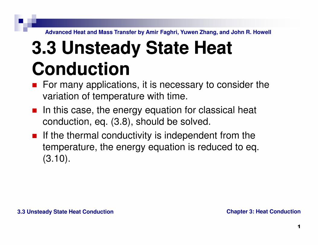
Consider an arbitrarily shaped object with volume V,
surface area As, and a uniform initial temperature of Ti as
shown in Fig. 3.15. At time t = 0, the arbitrarily shaped
object is exposed to a fluid with temperature of T∞ and
the convective heat transfer coefficient between the fluid
and the arbitrarily shaped object is h.
3.3.1 Lumped Analysis3.3.1 Lumped Analysis
T(t)
V
h,
T∞
As
Figure 3.15 Lumped capacitance method
Chapter 3: Heat Conduction
Advanced Heat and Mass Transfer by Amir Faghri, Yuwen Zhang, and John R. Howell
3.3 Unsteady State Heat Conduction
3
The convective heat transfer from the surface is
Similar to what we did for heat transfer from an extended
surface, the heat loss due to surface convection can be
treated as an equivalent heat source
Since the temperature is assumed to be uniform, the
energy equation becomes
(3.188)
which is subject to the following initial condition
(3.189)
( )s
q hA T T∞= −
( )s
hA T Tqq
V V
∞−′′′ = − = −
( )s
p
hA T TTc
t Vρ ∞−∂
= −∂
, 0iT T t= =
Chapter 3: Heat Conduction
Advanced Heat and Mass Transfer by Amir Faghri, Yuwen Zhang, and John R. Howell
3.3 Unsteady State Heat Conduction
4
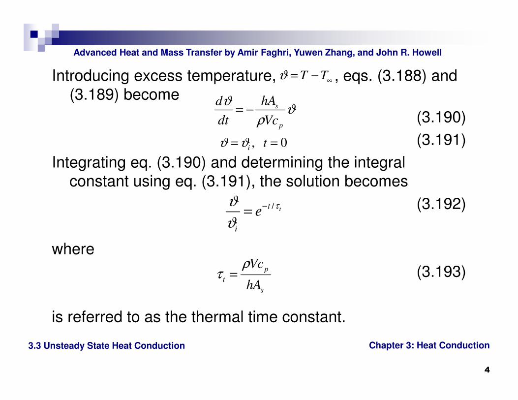
Introducing excess temperature, , eqs. (3.188) and
(3.189) become
(3.190)
(3.191)
Integrating eq. (3.190) and determining the integral
constant using eq. (3.191), the solution becomes
(3.192)
where
(3.193)
is referred to as the thermal time constant.
T Tϑ ∞= −
s
p
hAd
dt Vc
ϑϑ
ρ= −
, 0i tϑ ϑ= =
/ tt
i
eτϑ
ϑ−=
p
t
s
Vc
hA
ρτ =
Chapter 3: Heat Conduction
Advanced Heat and Mass Transfer by Amir Faghri, Yuwen Zhang, and John R. Howell
3.3 Unsteady State Heat Conduction
5
The cooling process requires transferring heat from the
center of the object to the surface and the heat is further
transferred away from the surface by convection. When
the lamped capacitance method is employed, it is
assumed that the conduction resistance within the object
is negligible compared with the convective thermal
resistance at the surface, therefore, the validity of the
lumped analysis depends on the relative thermal
resistances of conduction and convection. The
conduction thermal resistance can be expressed as
where Lc is the characteristic length and Ac is the area of
heat conduction.
c
cond
c
LR
kA=
Chapter 3: Heat Conduction
Advanced Heat and Mass Transfer by Amir Faghri, Yuwen Zhang, and John R. Howell
3.3 Unsteady State Heat Conduction
6
The convection thermal resistance at the surface is
Assuming , one can define the Biot number, Bi, as
the ratio of the conduction and convection thermal
resistances
(3.194)
If the characteristic length is chosen as , the
lumped capacitance method is valid when the Biot
number is less than 0.1, or the conduction thermal
resistance is one order of magnitude smaller than the
convection thermal resistance at the surface.
1conv
s
RhA
=
s cA A=
Bi= cond c
conv
R hL
R k�
/c sL V A=

Chapter 3: Heat Conduction
Advanced Heat and Mass Transfer by Amir Faghri, Yuwen Zhang, and John R. Howell
3.3 Unsteady State Heat Conduction
7
For the case that the Biot number is greater than 0.1, the
temperature distribution can no longer be treated as
uniform and the knowledge about the temperature
distribution is also of interest. We will now consider the
situation where temperature only varies in one spatial
dimension. Both homogeneous and nonhomogeneous
problem will be considered.
3.3.2 One Dimensional Transient
Systems
3.3.2 One Dimensional Transient
Systems
Chapter 3: Heat Conduction
Advanced Heat and Mass Transfer by Amir Faghri, Yuwen Zhang, and John R. Howell
3.3 Unsteady State Heat Conduction
8
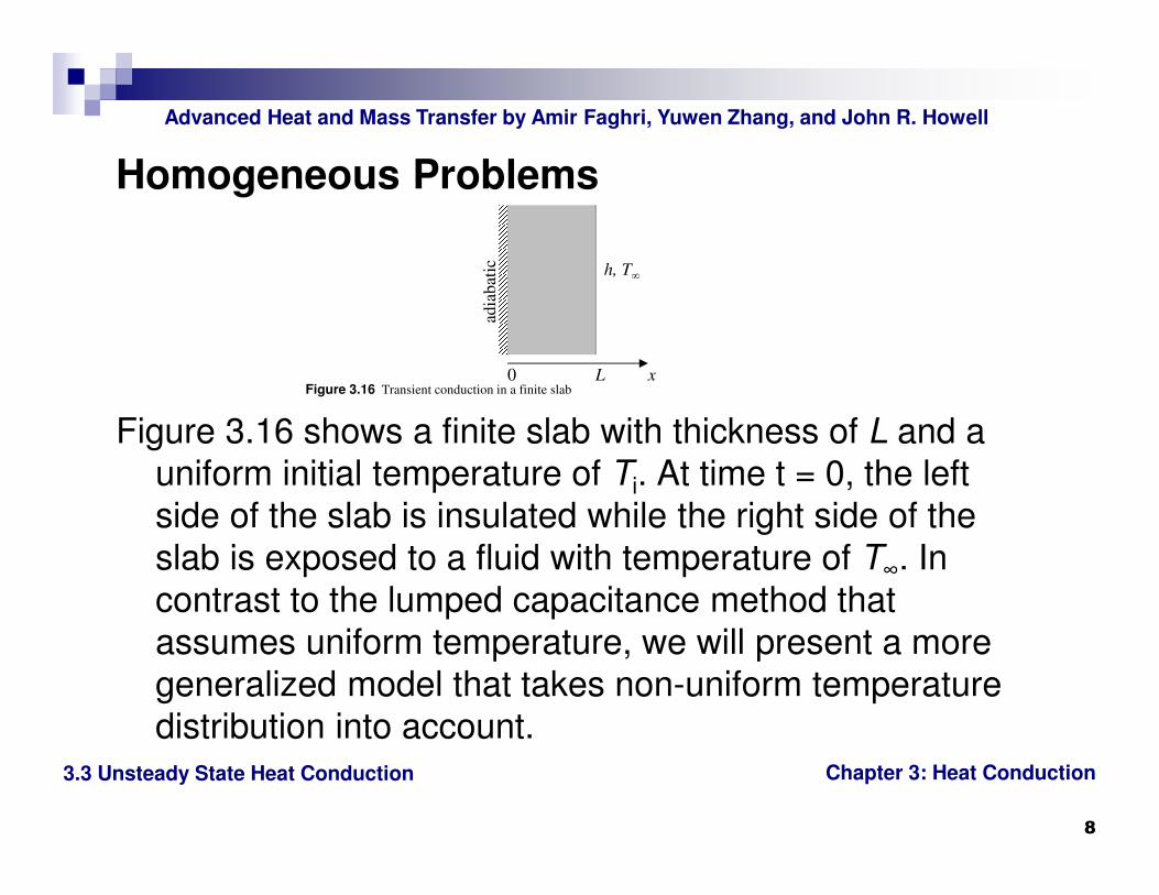
Homogeneous Problems
Figure 3.16 shows a finite slab with thickness of L and a
uniform initial temperature of Ti. At time t = 0, the left
side of the slab is insulated while the right side of the
slab is exposed to a fluid with temperature of T∞. In
contrast to the lumped capacitance method that
assumes uniform temperature, we will present a more
generalized model that takes non-uniform temperature
distribution into account.
h, T∞
Figure 3.16 Transient conduction in a finite slab0 xL
adia
bat
ic
Chapter 3: Heat Conduction
Advanced Heat and Mass Transfer by Amir Faghri, Yuwen Zhang, and John R. Howell
3.3 Unsteady State Heat Conduction
9
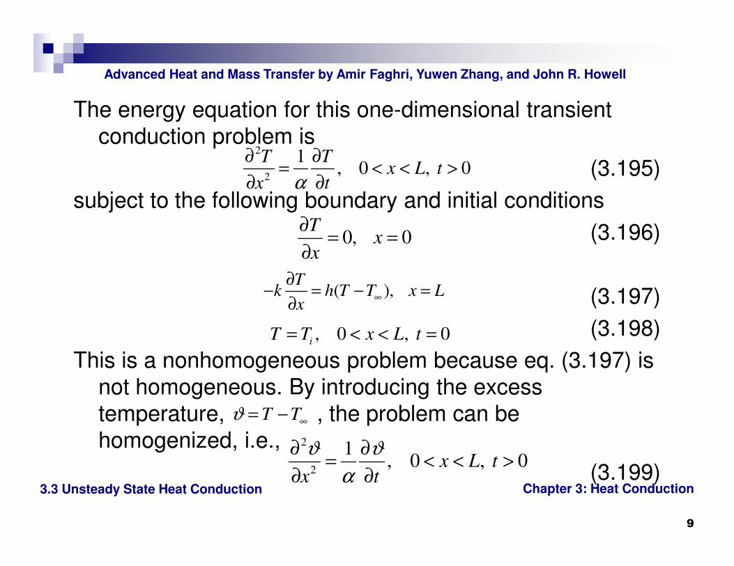
The energy equation for this one-dimensional transient
conduction problem is
(3.195)
subject to the following boundary and initial conditions
(3.196)
(3.197)
(3.198)
This is a nonhomogeneous problem because eq. (3.197) is
not homogeneous. By introducing the excess
temperature, , the problem can be
homogenized, i.e.,
(3.199)
2
2
1, 0 , 0
T Tx L t
x tα
∂ ∂= < < >
∂ ∂
0, 0T
xx
∂= =
∂
( ), T
k h T T x Lx
∞
∂− = − =
∂
, 0 , 0iT T x L t= < < =
T Tϑ ∞= −
2
2
1, 0 , 0x L t
x t
ϑ ϑ
α
∂ ∂= < < >
∂ ∂
Chapter 3: Heat Conduction
Advanced Heat and Mass Transfer by Amir Faghri, Yuwen Zhang, and John R. Howell
3.3 Unsteady State Heat Conduction
10
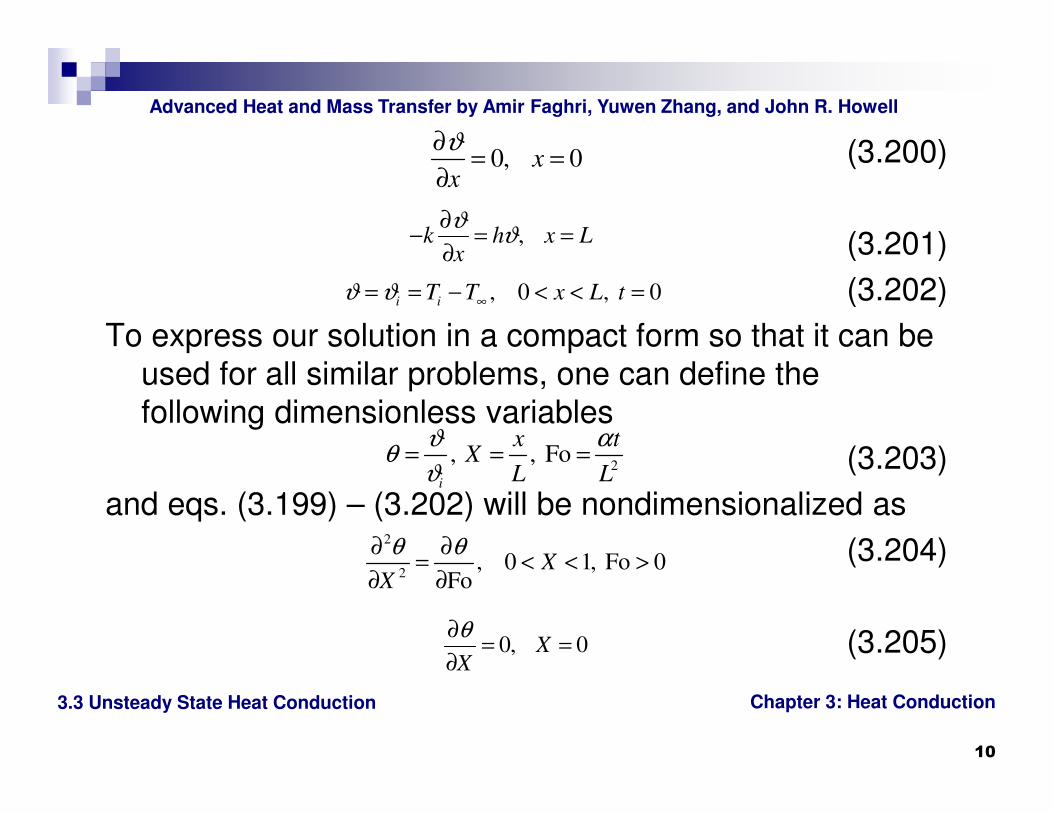
(3.200)
(3.201)
(3.202)
To express our solution in a compact form so that it can be
used for all similar problems, one can define the
following dimensionless variables
(3.203)
and eqs. (3.199) – (3.202) will be nondimensionalized as
(3.204)
(3.205)
0, 0xx
ϑ∂= =
∂
, k h x Lx
ϑϑ
∂− = =
∂
, 0 , 0i iT T x L tϑ ϑ ∞= = − < < =
2, , Fo
i
x tX
L L
ϑ αθ
ϑ= = =
2
2, 0 1, Fo 0
FoX
X
θ θ∂ ∂= < < >
∂ ∂
0, 0XX
θ∂= =
∂

Chapter 3: Heat Conduction
Advanced Heat and Mass Transfer by Amir Faghri, Yuwen Zhang, and John R. Howell
3.3 Unsteady State Heat Conduction
11
(3.206)
(3.207)
This problem can be solved using the method of separation
of variables. Assuming that the temperature can be
expressed as
(3.208)
where are functions of X and Fo, respectively, eq.
(3.204) becomes
Since the left hand side is a function of X only and the right-
hand side of the above equation is a function of Fo only,
both sides must be equal to a separation constant, , i.e.,
Bi , X 1X
θθ
∂− = =
∂
1, 0 1, Fo 0Xθ = < < =
( ,Fo) ( ) (Fo)X Xθ = Θ Γ
and Θ Γ
( ) (Fo)
( ) (Fo)
X
X
′′ ′Θ Γ=
Θ Γ
Chapter 3: Heat Conduction
Advanced Heat and Mass Transfer by Amir Faghri, Yuwen Zhang, and John R. Howell
3.3 Unsteady State Heat Conduction
12
(3.209)
The separation constant µ can be either a real or a
complex number. The solution of from eq. (3.209) will
be . If is a positive real number, we will have
when , which does not make sense, therefore,
cannot be a positive real number. If is zero, we will
have , and is a linear function of X only. The
final solution for will also be a linear function of X only,
which does not make sense either. It can also be shown
that the separation constant cannot be a complex
number, therefore, the separation variable has to be a
negative real number.
( ) (Fo)
( ) (Fo)
X
Xµ
′′ ′Θ Γ= =
Θ Γ
ΓFo
eµΓ = µ Γ → ∞
Fo → ∞ µµ
constΓ = Θ
θ

Chapter 3: Heat Conduction
Advanced Heat and Mass Transfer by Amir Faghri, Yuwen Zhang, and John R. Howell
3.3 Unsteady State Heat Conduction
13
If we represent this negative number by , eqs. (3.209)
can be rewritten as the following two equations
(3.210)
(3.211)
The general solutions of eqs. (3.210) and (3.211) are
(3.212)
(3.213)
where C1, C2, and C3 are integral constants.
Substituting eq. (3.208) into eqs. (3.205) and (3.206), the
following boundary conditions of eq. (3.210) are obtained
(3.214)
(3.215)
2µ λ= −
20λ′′Θ + Θ =
2 0λ′Γ + Γ =
1 2cos sinC X C Xλ λΘ = +2Fo
3C e λ−Γ =
(0) 0′Θ =
(1) Bi (1)′−Θ = Θ
Chapter 3: Heat Conduction
Advanced Heat and Mass Transfer by Amir Faghri, Yuwen Zhang, and John R. Howell
3.3 Unsteady State Heat Conduction
14
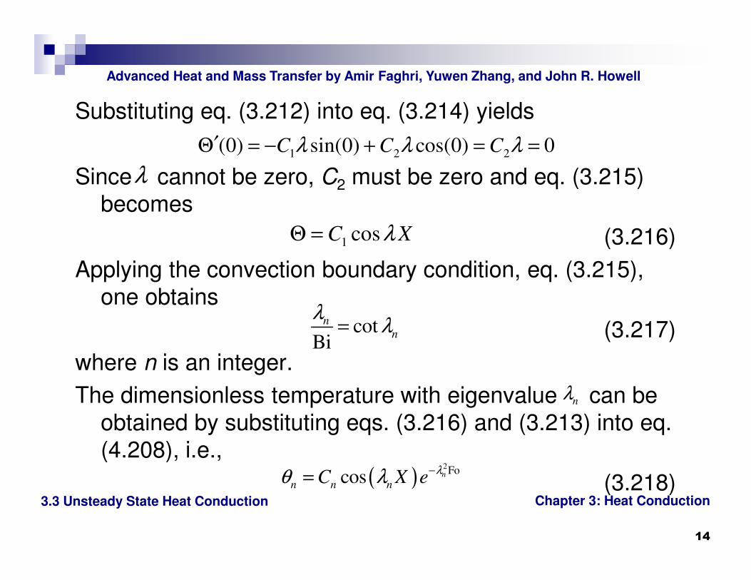
Substituting eq. (3.212) into eq. (3.214) yields
Since cannot be zero, C2 must be zero and eq. (3.215)
becomes
(3.216)
Applying the convection boundary condition, eq. (3.215),
one obtains
(3.217)
where n is an integer.
The dimensionless temperature with eigenvalue can be
obtained by substituting eqs. (3.216) and (3.213) into eq.
(4.208), i.e.,
(3.218)
1 2 2(0) sin(0) cos(0) 0C C Cλ λ λ′Θ = − + = =
λ
1 cosC XλΘ =
cotBi
n
n
λλ=
nλ
( )2Fo
cos n
n n nC X e
λθ λ −=
Chapter 3: Heat Conduction
Advanced Heat and Mass Transfer by Amir Faghri, Yuwen Zhang, and John R. Howell
3.3 Unsteady State Heat Conduction
15
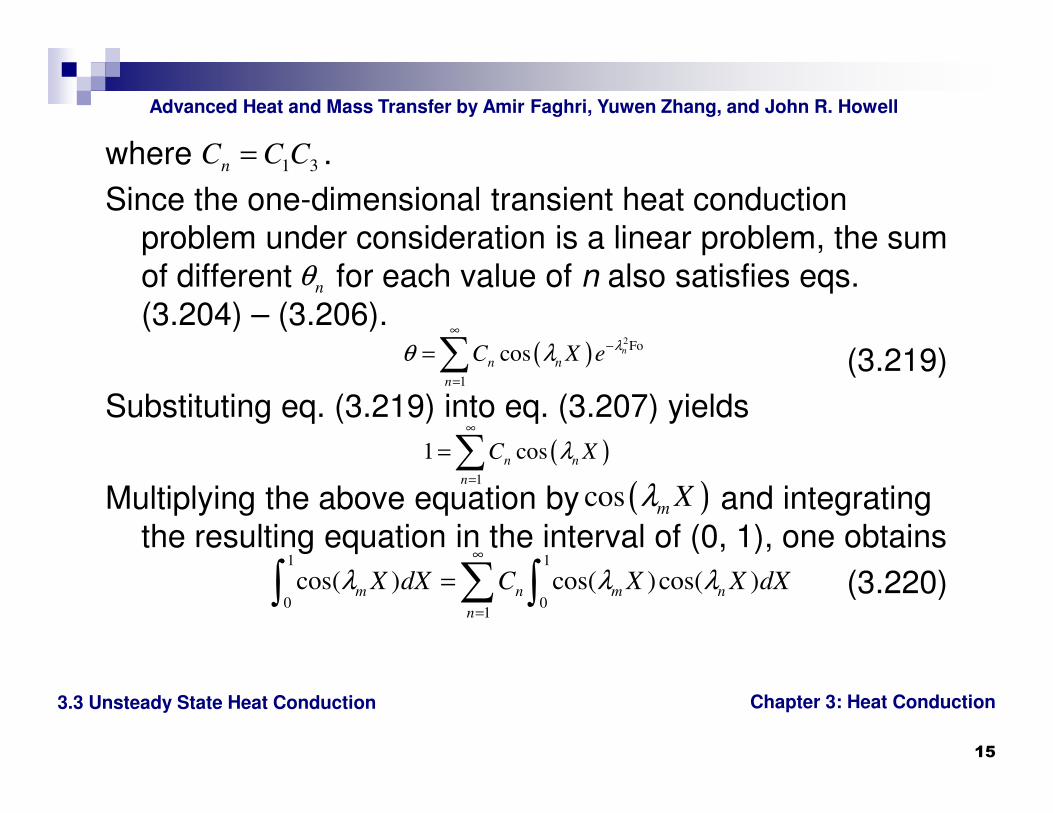
where .
Since the one-dimensional transient heat conduction
problem under consideration is a linear problem, the sum
of different for each value of n also satisfies eqs.
(3.204) – (3.206).
(3.219)
Substituting eq. (3.219) into eq. (3.207) yields
Multiplying the above equation by and integrating
the resulting equation in the interval of (0, 1), one obtains
(3.220)
1 3nC C C=
nθ
( )2Fo
1
cos n
n n
n
C X eλθ λ
∞−
=
=∑
( )1
1 cosn n
n
C Xλ∞
=
=∑( )cos m Xλ
1 1
0 01
cos( ) cos( )cos( )m n m n
n
X dX C X X dXλ λ λ∞
=
=∑∫ ∫

Chapter 3: Heat Conduction
Advanced Heat and Mass Transfer by Amir Faghri, Yuwen Zhang, and John R. Howell
3.3 Unsteady State Heat Conduction
16
The integral in the right-hand side of eq. (3.133) can be
evaluated as
(3.221)
Equation (3.217) can be rewritten as
Similarly, for eigenvalue , we have
Combining the above two equations, we have
or
2 21
0
sin cos cos sin,
cos( )cos( )sin 21
, 2 2
m m n n m n
m n
m n
m
m
m
m n
X X dX
m n
λ λ λ λ λ λ
λ λλ λ
λλ
λ
−≠ −
= + =
∫
Bi tann n
λ λ=
mλ
Bi tanm mλ λ=
tan tan 0m m n n
λ λ λ λ− =
sin cos cos sin 0m m n n m nλ λ λ λ λ λ− =
Chapter 3: Heat Conduction
Advanced Heat and Mass Transfer by Amir Faghri, Yuwen Zhang, and John R. Howell
3.3 Unsteady State Heat Conduction
17
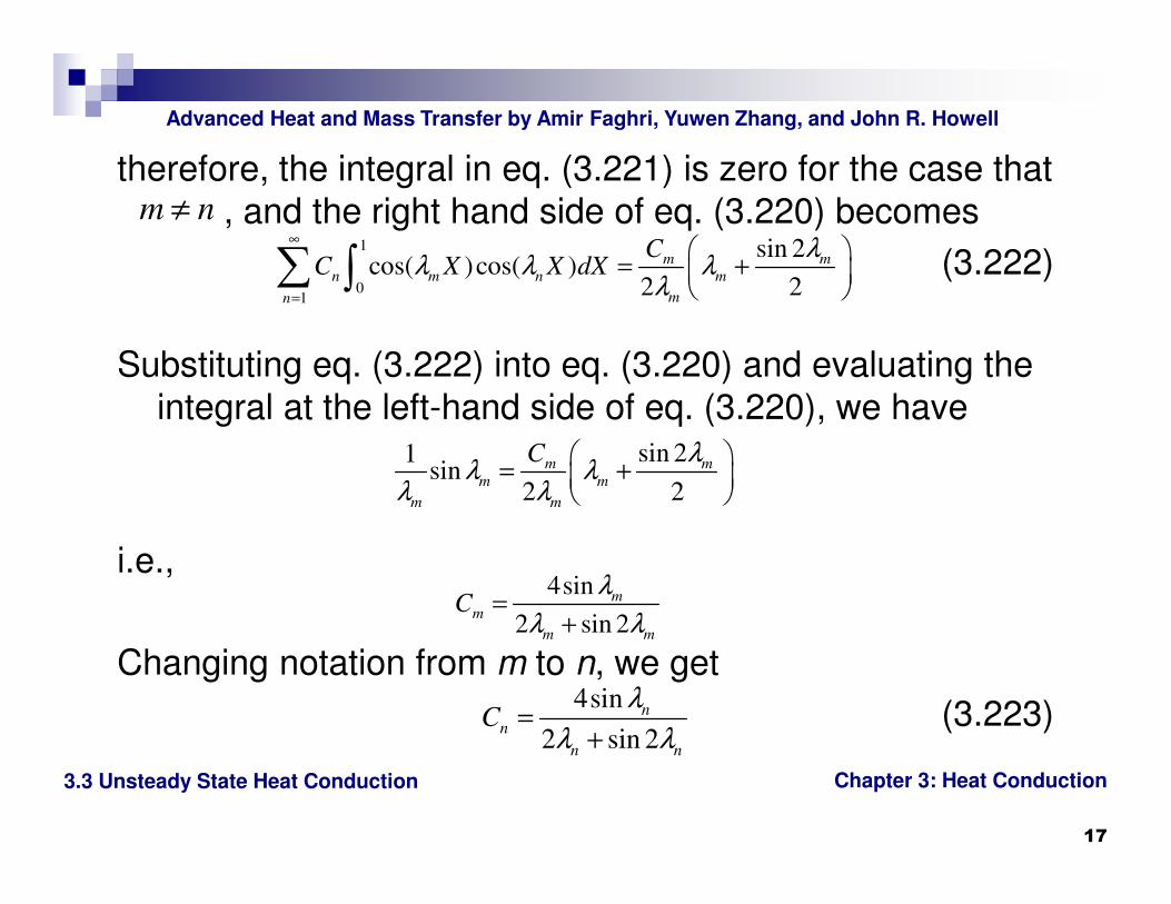
therefore, the integral in eq. (3.221) is zero for the case that
, and the right hand side of eq. (3.220) becomes
(3.222)
Substituting eq. (3.222) into eq. (3.220) and evaluating the
integral at the left-hand side of eq. (3.220), we have
i.e.,
Changing notation from m to n, we get
(3.223)
m n≠1
01
sin 2cos( )cos( )
2 2
m m
n m n m
mn
CC X X dX
λλ λ λ
λ
∞
=
= +
∑ ∫
sin 21sin
2 2
m m
m m
m m
C λλ λ
λ λ
= +
4sin
2 sin 2
mm
m m
Cλ
λ λ=
+
4sin
2 sin 2
n
n
n n
Cλ
λ λ=
+
Chapter 3: Heat Conduction
Advanced Heat and Mass Transfer by Amir Faghri, Yuwen Zhang, and John R. Howell
3.3 Unsteady State Heat Conduction
18
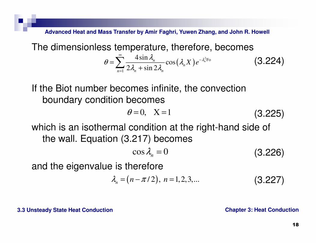
The dimensionless temperature, therefore, becomes
(3.224)
If the Biot number becomes infinite, the convection
boundary condition becomes
(3.225)
which is an isothermal condition at the right-hand side of
the wall. Equation (3.217) becomes
(3.226)
and the eigenvalue is therefore
(3.227)
( )2Fo
1
4sincos
2 sin 2nn
n
n nn
X eλλ
θ λλ λ
∞−
=
=+∑
0, X 1θ = =
cos 0nλ =
( )/ 2 , 1,2,3,...n n nλ π= − =
Chapter 3: Heat Conduction
Advanced Heat and Mass Transfer by Amir Faghri, Yuwen Zhang, and John R. Howell
3.3 Unsteady State Heat Conduction
19
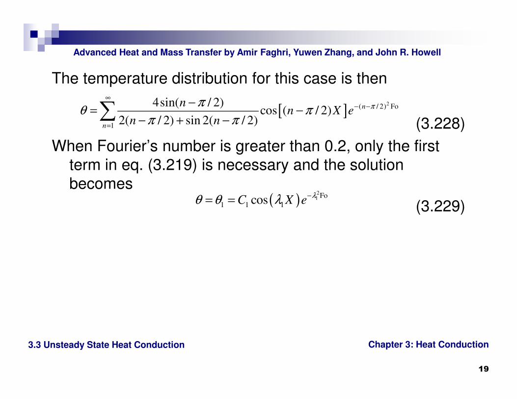
The temperature distribution for this case is then
(3.228)
When Fourier’s number is greater than 0.2, only the first
term in eq. (3.219) is necessary and the solution
becomes
(3.229)
[ ]2( / 2) Fo
1
4sin( / 2)cos ( / 2)
2( / 2) sin 2( / 2)
n
n
nn X e
n n
ππθ π
π π
∞− −
=
−= −
− + −∑
( )2
1 Fo
1 1 1cosC X eλθ θ λ −= =
Chapter 3: Heat Conduction
Advanced Heat and Mass Transfer by Amir Faghri, Yuwen Zhang, and John R. Howell
3.3 Unsteady State Heat Conduction
20
� Example 3.3
A long cylinder with radius of ro and a uniform initial
temperature of Ti is exposed to a fluid with temperature
of T∞. The convective heat transfer coefficient between
the fluid and cylinder is h. Assuming that there is no
internal heat generation and constant thermophysical
properties, obtain the transient temperature distribution
in the cylinder.
Chapter 3: Heat Conduction
Advanced Heat and Mass Transfer by Amir Faghri, Yuwen Zhang, and John R. Howell
3.3 Unsteady State Heat Conduction
21
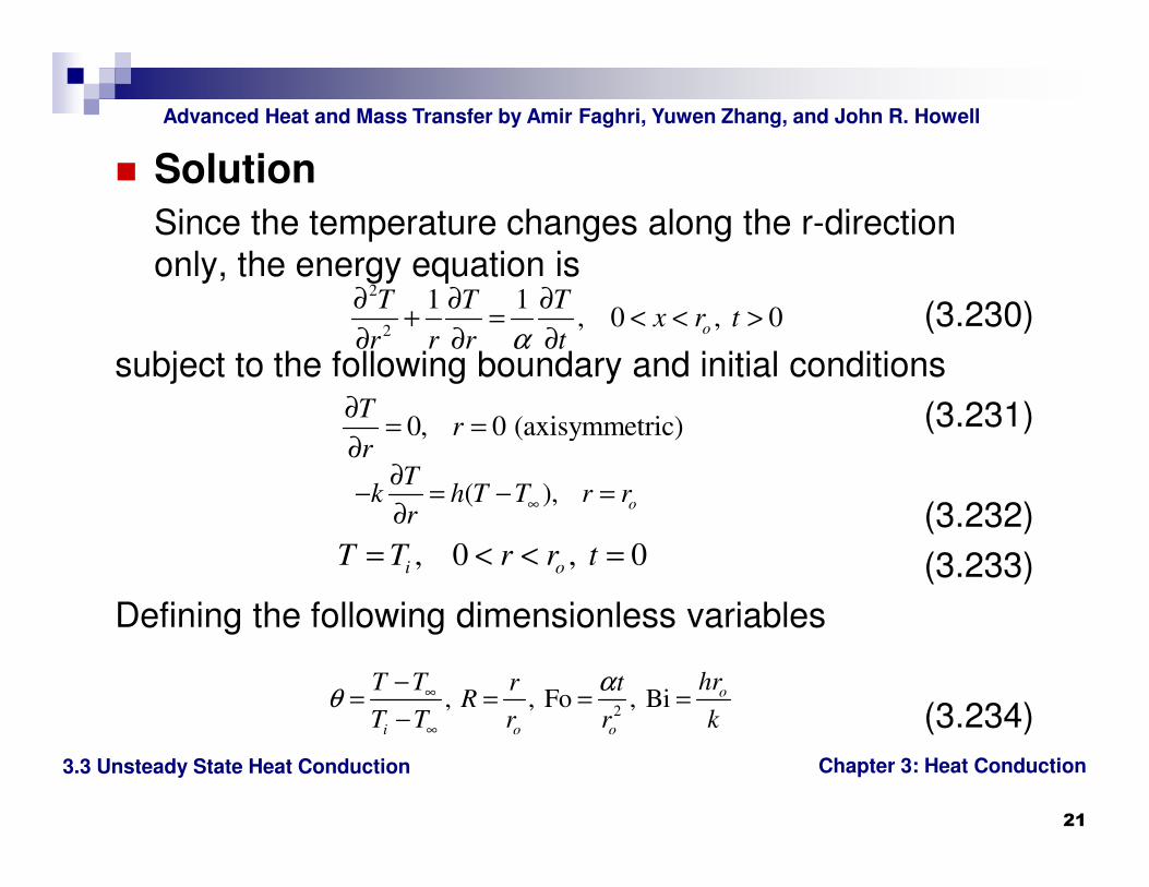
� Solution
Since the temperature changes along the r-direction
only, the energy equation is
(3.230)
subject to the following boundary and initial conditions
(3.231)
(3.232)
(3.233)
Defining the following dimensionless variables
(3.234)
2
2
1 1, 0 , 0o
T T Tx r t
r r r tα
∂ ∂ ∂+ = < < >
∂ ∂ ∂
0, 0 (axisymmetric)T
rr
∂= =
∂
( ), o
Tk h T T r r
r∞
∂− = − =
∂
, 0 , 0i oT T r r t= < < =
2, , Fo , Bi o
i o o
hrT T r tR
T T r r k
αθ ∞
∞
−= = = =
−

Chapter 3: Heat Conduction
Advanced Heat and Mass Transfer by Amir Faghri, Yuwen Zhang, and John R. Howell
3.3 Unsteady State Heat Conduction
22
eqs. (3.230) – (4.233) will be nondimensionalized as
(3.235)
(3.236)
(3.237)
(3.238)
Assuming that the temperature can be expressed as
(3.239)
and substituting eq. (3.239) into eq. (3.235), one obtains
(3.240)
2
2
1, 0 1, Fo 0
FoR
R R R
θ θ θ∂ ∂ ∂+ = < < >
∂ ∂ ∂
0, 0RR
θ∂= =
∂
Bi , R 1R
θθ
∂− = =
∂
1, 0 1, Fo 0Rθ = < < =
( ,Fo) ( ) (Fo)R Rθ = Θ Γ
21 1
Rλ
′Γ ′′ ′Θ + Θ = = − Θ Γ

Chapter 3: Heat Conduction
Advanced Heat and Mass Transfer by Amir Faghri, Yuwen Zhang, and John R. Howell
3.3 Unsteady State Heat Conduction
23
which can be rewritten as the following two equations
(3.241)
(3.242)
Equation (3.101) is a Bessel’s equation of zero order and
has the following general solution
(3.243)
where J0 and Y0 are the Bessel’s function of the first and
second kind, respectively. The general solution of eq.
(3.242) is
(3.244)
where C1, C2, and C3 are integral constants.
210
Rλ′′ ′Θ + Θ + Θ =
2 0λ′Γ + Γ =
1 0 2 0( ) ( ) ( )R C J R C Y Rλ λΘ = +
2Fo
3C eλ−Γ =
Chapter 3: Heat Conduction
Advanced Heat and Mass Transfer by Amir Faghri, Yuwen Zhang, and John R. Howell
3.3 Unsteady State Heat Conduction
24
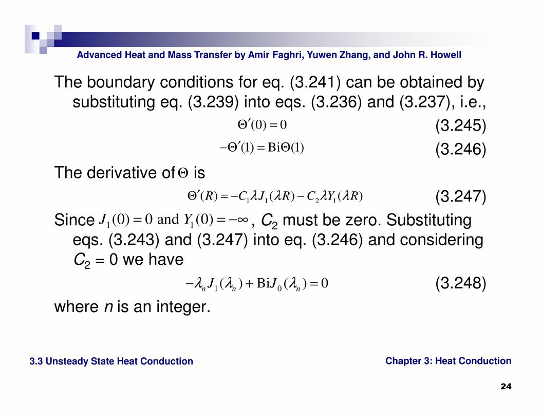
The boundary conditions for eq. (3.241) can be obtained by
substituting eq. (3.239) into eqs. (3.236) and (3.237), i.e.,
(3.245)
(3.246)
The derivative of is
(3.247)
Since , C2 must be zero. Substituting
eqs. (3.243) and (3.247) into eq. (3.246) and considering
C2 = 0 we have
(3.248)
where n is an integer.
(0) 0′Θ =
(1) Bi (1)′−Θ = Θ
Θ
1 1 2 1( ) ( ) ( )R C J R C Y Rλ λ λ λ′Θ = − −
1 1(0) 0 and (0)J Y= = −∞
1 0( ) Bi ( ) 0n n nJ Jλ λ λ− + =
Chapter 3: Heat Conduction
Advanced Heat and Mass Transfer by Amir Faghri, Yuwen Zhang, and John R. Howell
3.3 Unsteady State Heat Conduction
25
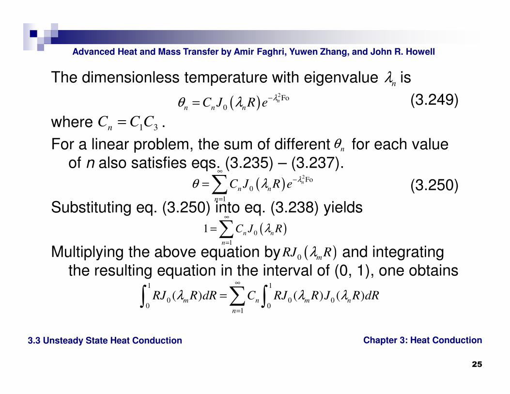
The dimensionless temperature with eigenvalue is
(3.249)
where .
For a linear problem, the sum of different for each value
of n also satisfies eqs. (3.235) – (3.237).
(3.250)
Substituting eq. (3.250) into eq. (3.238) yields
Multiplying the above equation by and integrating
the resulting equation in the interval of (0, 1), one obtains
nλ
( )2Fo
0n
n n nC J R eλθ λ −=
1 3nC C C=
nθ
( )2Fo
0
1
n
n n
n
C J R eλθ λ
∞−
=
=∑
( )0
1
1 n n
n
C J Rλ∞
=
=∑( )0 mRJ Rλ
1 1
0 0 00 0
1
( ) ( ) ( )m n m n
n
RJ R dR C RJ R J R dRλ λ λ∞
=
=∑∫ ∫
Chapter 3: Heat Conduction
Advanced Heat and Mass Transfer by Amir Faghri, Yuwen Zhang, and John R. Howell
3.3 Unsteady State Heat Conduction
26
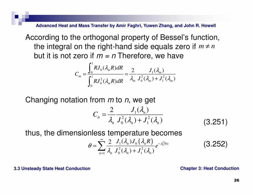
According to the orthogonal property of Bessel’s function,
the integral on the right-hand side equals zero if
but it is not zero if m = n Therefore, we have
Changing notation from m to n, we get
(3.251)
thus, the dimensionless temperature becomes
(3.252)
m n≠
1
00 1
1 2 22 0 10
0
( ) ( )2
( ) ( )( )
mm
m
m m mm
RJ R dR JC
J JRJ R dR
λ λ
λ λ λλ= =
+
∫∫
1
2 2
0 1
( )2
( ) ( )
n
n
n n n
JC
J J
λ
λ λ λ=
+
( ) 21 0 Fo
2 2
0 11
( )2
( ) ( )nn n
n n nn
J J Re
J J
λλ λθ
λ λ λ
∞−
=
=+∑
Chapter 3: Heat Conduction
Advanced Heat and Mass Transfer by Amir Faghri, Yuwen Zhang, and John R. Howell
3.3 Unsteady State Heat Conduction
27
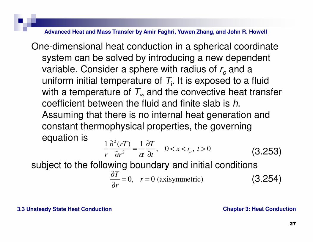
One-dimensional heat conduction in a spherical coordinate
system can be solved by introducing a new dependent
variable. Consider a sphere with radius of ro and a
uniform initial temperature of Ti. It is exposed to a fluid
with a temperature of T∞ and the convective heat transfer
coefficient between the fluid and finite slab is h.
Assuming that there is no internal heat generation and
constant thermophysical properties, the governing
equation is
(3.253)
subject to the following boundary and initial conditions
(3.254)
2
2
1 ( ) 1, 0 , 0o
rT Tx r t
r r tα
∂ ∂= < < >
∂ ∂
0, 0 (axisymmetric)T
rr
∂= =
∂

Chapter 3: Heat Conduction
Advanced Heat and Mass Transfer by Amir Faghri, Yuwen Zhang, and John R. Howell
3.3 Unsteady State Heat Conduction
28
(3.255)
(3.256)
By using the same dimensionless variables defined in eq.
(3.234), eqs. (3.253) – (3.256) can be
nondimensionalized as
(3.257)
(3.258)
(3.259)
(3.260)
Defining a new dependent variable
(3.261)
( ), o
Tk h T T r r
r∞
∂− = − =
∂, 0 , 0i oT T r r t= < < =
2
2
1 ( ), 0 1, Fo 0
Fo
RR
R R
θ θ∂ ∂= < < >
∂ ∂
0, 0RR
θ∂= =
∂
Bi , R 1R
θθ
∂− = =
∂
1, 0 1, Fo 0Rθ = < < =
U Rθ=
Chapter 3: Heat Conduction
Advanced Heat and Mass Transfer by Amir Faghri, Yuwen Zhang, and John R. Howell
3.3 Unsteady State Heat Conduction
29
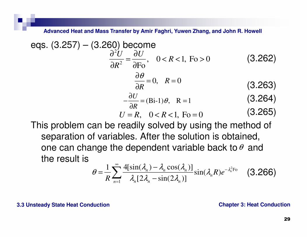
eqs. (3.257) – (3.260) become
(3.262)
(3.263)
(3.264)
(3.265)
This problem can be readily solved by using the method of
separation of variables. After the solution is obtained,
one can change the dependent variable back to and
the result is
(3.266)
2
2, 0 1, Fo 0
Fo
U UR
R
∂ ∂= < < >
∂ ∂
0, 0RR
θ∂= =
∂
(Bi-1) , R 1U
Rθ
∂− = =
∂, 0 1, Fo 0U R R= < < =
θ
2Fo
1
4[sin( ) cos( )]1sin( )
[2 sin(2 )]nn n n
n
n n nn
R eR
λλ λ λθ λ
λ λ λ
∞−
=
−=
−∑
Chapter 3: Heat Conduction
Advanced Heat and Mass Transfer by Amir Faghri, Yuwen Zhang, and John R. Howell
3.3 Unsteady State Heat Conduction
30
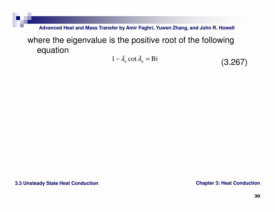
where the eigenvalue is the positive root of the following
equation
(3.267)1 cot Bin n
λ λ− =
Chapter 3: Heat Conduction
Advanced Heat and Mass Transfer by Amir Faghri, Yuwen Zhang, and John R. Howell
3.3 Unsteady State Heat Conduction
31
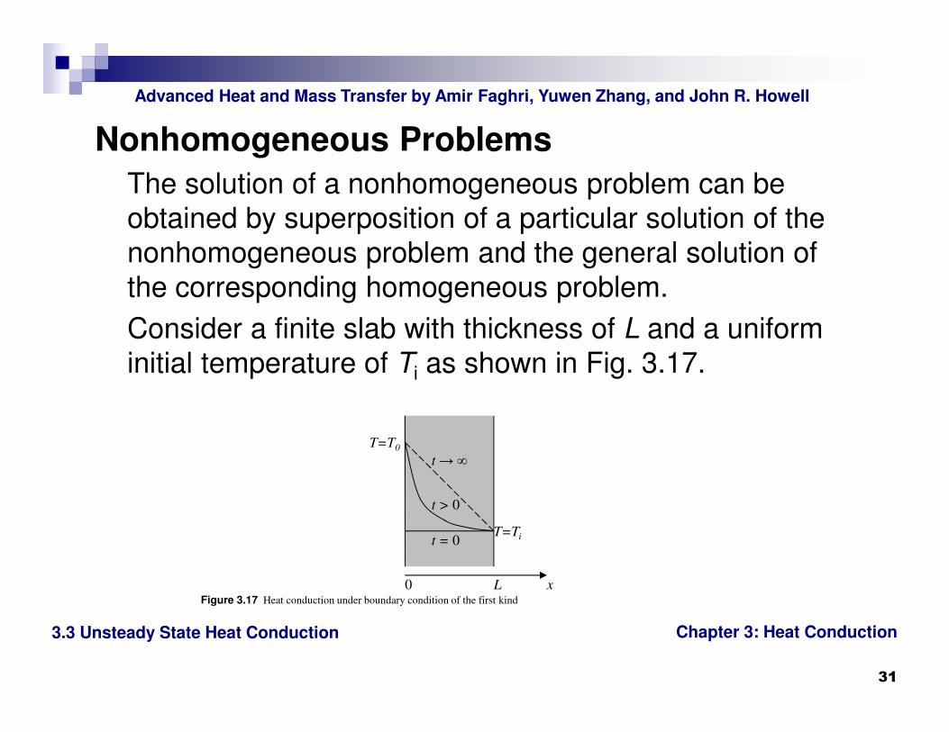
Nonhomogeneous Problems
The solution of a nonhomogeneous problem can be
obtained by superposition of a particular solution of the
nonhomogeneous problem and the general solution of
the corresponding homogeneous problem.
Consider a finite slab with thickness of L and a uniform
initial temperature of Ti as shown in Fig. 3.17.
T=Ti
Figure 3.17 Heat conduction under boundary condition of the first kind
0 xL
T=T0
t = 0
t > 0
t → ∞
Chapter 3: Heat Conduction
Advanced Heat and Mass Transfer by Amir Faghri, Yuwen Zhang, and John R. Howell
3.3 Unsteady State Heat Conduction
32
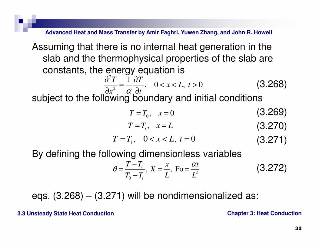
Assuming that there is no internal heat generation in the
slab and the thermophysical properties of the slab are
constants, the energy equation is
(3.268)
subject to the following boundary and initial conditions
(3.269)
(3.270)
(3.271)
By defining the following dimensionless variables
(3.272)
eqs. (3.268) – (3.271) will be nondimensionalized as:
2
2
1, 0 , 0
T Tx L t
x tα
∂ ∂= < < >
∂ ∂
0 , 0T T x= =
, i
T T x L= =
, 0 , 0iT T x L t= < < =
2
0
, , Foi
i
T T x tX
T T L L
αθ
−= = =
−
Chapter 3: Heat Conduction
Advanced Heat and Mass Transfer by Amir Faghri, Yuwen Zhang, and John R. Howell
3.3 Unsteady State Heat Conduction
33
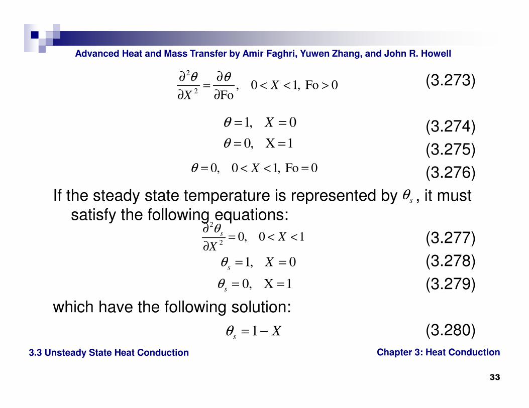
(3.273)
(3.274)
(3.275)
(3.276)
If the steady state temperature is represented by , it must
satisfy the following equations:
(3.277)
(3.278)
(3.279)
which have the following solution:
(3.280)
2
2, 0 1, Fo 0
FoX
X
θ θ∂ ∂= < < >
∂ ∂
1, 0Xθ = =
0, X 1θ = =
0, 0 1, Fo 0Xθ = < < =
sθ
2
20, 0 1s X
X
θ∂= < <
∂
1, 0s
Xθ = =
0, X 1s
θ = =
1s Xθ = −
Chapter 3: Heat Conduction
Advanced Heat and Mass Transfer by Amir Faghri, Yuwen Zhang, and John R. Howell
3.3 Unsteady State Heat Conduction
34
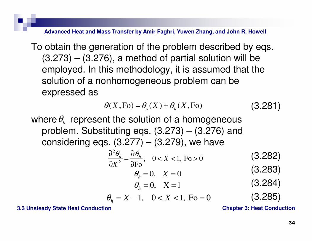
To obtain the generation of the problem described by eqs.
(3.273) – (3.276), a method of partial solution will be
employed. In this methodology, it is assumed that the
solution of a nonhomogeneous problem can be
expressed as
(3.281)
where represent the solution of a homogeneous
problem. Substituting eqs. (3.273) – (3.276) and
considering eqs. (3.277) – (3.279), we have
(3.282)
(3.283)
(3.284)
(3.285)
( ,Fo) ( ) ( ,Fo)s hX X Xθ θ θ= +
hθ
2
2, 0 1, Fo 0
Fo
h h XX
θ θ∂ ∂= < < >
∂ ∂
0, 0h Xθ = =
0, X 1hθ = =
1, 0 1, Fo 0h X Xθ = − < < =
Chapter 3: Heat Conduction
Advanced Heat and Mass Transfer by Amir Faghri, Yuwen Zhang, and John R. Howell
3.3 Unsteady State Heat Conduction
35
which represent a new homogeneous problem. This
problem can be solved using the method of separation of
variables and the result is
(3.286)
The solution of the nonhomogeneous problem thus
becomes
(3.287)
2( ) Fo
1
2 sin( ) n
h
n
n Xe
n
ππθ
π
∞−
=
= − ∑
2( ) Fo
1
2 sin( )1 n
n
n XX e
n
ππθ
π
∞−
=
= − − ∑
Chapter 3: Heat Conduction
Advanced Heat and Mass Transfer by Amir Faghri, Yuwen Zhang, and John R. Howell
3.3 Unsteady State Heat Conduction
36
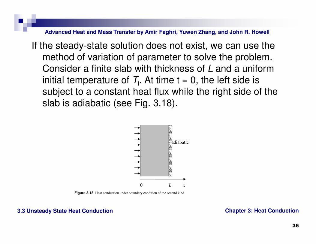
If the steady-state solution does not exist, we can use the
method of variation of parameter to solve the problem.
Consider a finite slab with thickness of L and a uniform
initial temperature of Ti. At time t = 0, the left side is
subject to a constant heat flux while the right side of the
slab is adiabatic (see Fig. 3.18).
Figure 3.18 Heat conduction under boundary condition of the second kind
0 xL
adiabatic

Chapter 3: Heat Conduction
Advanced Heat and Mass Transfer by Amir Faghri, Yuwen Zhang, and John R. Howell
3.3 Unsteady State Heat Conduction
37
Assuming that there is no internal heat generation in the
slab and the thermophysical properties of the slab are
constants, the energy equation is
(3.288)
subject to the following boundary and initial conditions
(3.289)
(3.290)
(3.291)
By defining the following dimensionless variables
(3.292)
eqs. (3.268) – (3.271) will be nondimensionalized as:
2
2
1, 0 , 0
T Tx L t
x tα
∂ ∂= < < >
∂ ∂
0 , 0T
k q xx
∂′′− = =
∂
0, T
x Lx
∂= =
∂
, 0 , 0iT T x L t= < < =
2
0
, , Fo/
iT T x tX
q L k L L
αθ
−= = =
′′
Chapter 3: Heat Conduction
Advanced Heat and Mass Transfer by Amir Faghri, Yuwen Zhang, and John R. Howell
3.3 Unsteady State Heat Conduction
38
(3.293)
(3.294)
(3.295)
(3.296)
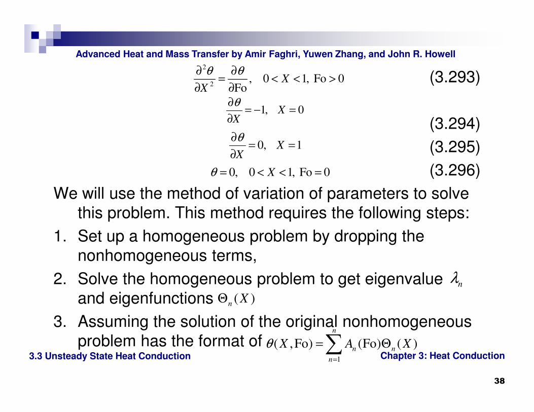
We will use the method of variation of parameters to solve
this problem. This method requires the following steps:
1. Set up a homogeneous problem by dropping the
nonhomogeneous terms,
2. Solve the homogeneous problem to get eigenvalue
and eigenfunctions
3. Assuming the solution of the original nonhomogeneous
problem has the format of
2
2, 0 1, Fo 0
FoX
X
θ θ∂ ∂= < < >
∂ ∂
1, 0XX
θ∂= − =
∂
0, 1XX
θ∂= =
∂
0, 0 1, Fo 0Xθ = < < =
( )n XΘnλ
1
( ,Fo) (Fo) ( )
n
n n
n
X A Xθ=
= Θ∑
Chapter 3: Heat Conduction
Advanced Heat and Mass Transfer by Amir Faghri, Yuwen Zhang, and John R. Howell
3.3 Unsteady State Heat Conduction
39
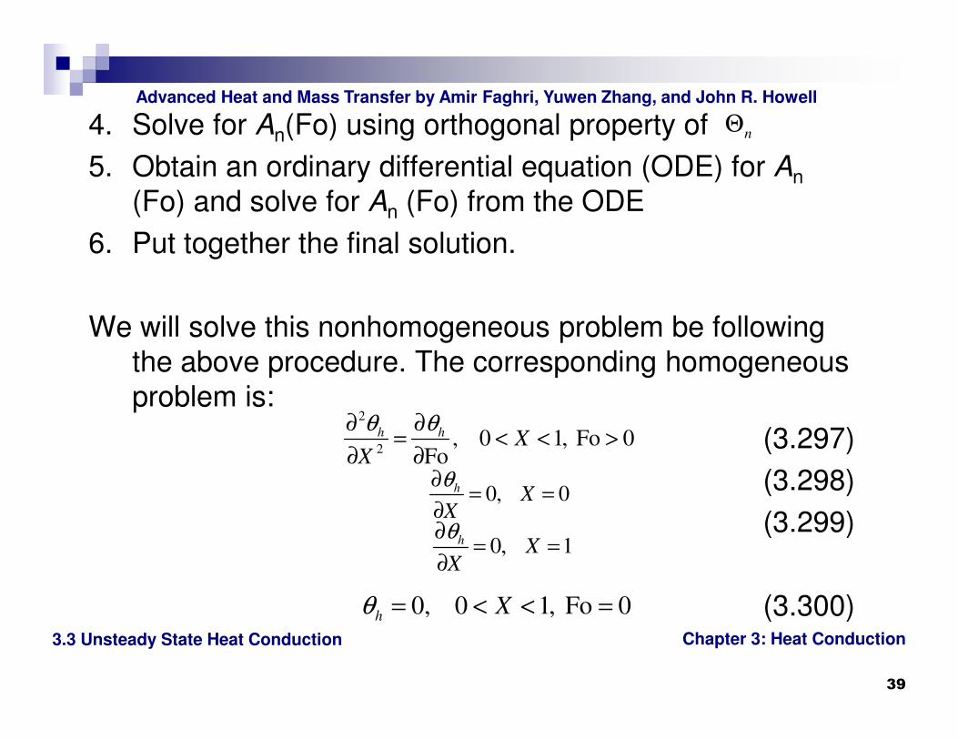
4. Solve for An(Fo) using orthogonal property of
5. Obtain an ordinary differential equation (ODE) for An
(Fo) and solve for An (Fo) from the ODE
6. Put together the final solution.
We will solve this nonhomogeneous problem be following
the above procedure. The corresponding homogeneous
problem is:
(3.297)
(3.298)
(3.299)
(3.300)
nΘ
2
2, 0 1, Fo 0
Fo
h h XX
θ θ∂ ∂= < < >
∂ ∂
0, 0h XX
θ∂= =
∂
0, 1h XX
θ∂= =
∂
0, 0 1, Fo 0h Xθ = < < =
Chapter 3: Heat Conduction
Advanced Heat and Mass Transfer by Amir Faghri, Yuwen Zhang, and John R. Howell
3.3 Unsteady State Heat Conduction
40
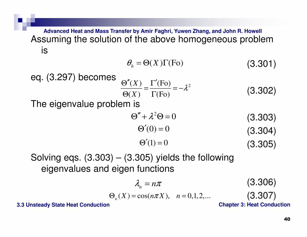
Assuming the solution of the above homogeneous problem
is
(3.301)
eq. (3.297) becomes
(3.302)
The eigenvalue problem is
(3.303)
(3.304)
(3.305)
Solving eqs. (3.303) – (3.305) yields the following
eigenvalues and eigen functions
(3.306)
(3.307)
( ) (Fo)h Xθ = Θ Γ
2( ) (Fo)
( ) (Fo)
X
Xλ
′′ ′Θ Γ= = −
Θ Γ
2 0λ′′Θ + Θ =
(0) 0′Θ =
(1) 0′Θ =
n nλ π=
( ) cos( ), 0,1,2,...n X n X nπΘ = =

Chapter 3: Heat Conduction
Advanced Heat and Mass Transfer by Amir Faghri, Yuwen Zhang, and John R. Howell
3.3 Unsteady State Heat Conduction
41
Now, let us assume that the solution of the original
nonhomogeneous problem is
(3.308)
Multiplying eq. (3.308) by and integrating the
resulting equation in the interval of (0, 1), one obtains
(3.309)
The integral on the right-hand side of eq. (3.309) can be
evaluated as
(3.310)
thus, eq. (3.309) becomes
(3.311)
( )0
( ,Fo) (Fo)cosn
n
X A n Xθ π∞
=
=∑( )cos m Xπ
1 1
0 01
( ,Fo)cos( ) cos( )cos( )n
n
X m X dX A m X n X dXθ π π π∞
=
=∑∫ ∫
1
0
0,
cos( )cos( ) 1/ 2, 0
1, 0
m n
m X n X dX m n
m n
π π
≠
= = ≠ = =
∫
1
00
(Fo) ( ,Fo) , 0A X dX mθ= =∫
Chapter 3: Heat Conduction
Advanced Heat and Mass Transfer by Amir Faghri, Yuwen Zhang, and John R. Howell
3.3 Unsteady State Heat Conduction
42
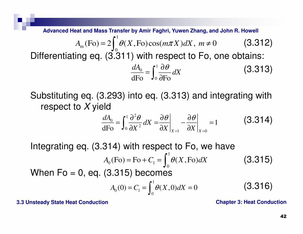
(3.312)
Differentiating eq. (3.311) with respect to Fo, one obtains:
(3.313)
Substituting eq. (3.293) into eq. (3.313) and integrating with
respect to X yield
(3.314)
Integrating eq. (3.314) with respect to Fo, we have
(3.315)
When Fo = 0, eq. (3.315) becomes
(3.316)
1
m0
(Fo) 2 ( ,Fo)cos( ) , 0A X m X dX mθ π= ≠∫1
0
0dFo Fo
dAdX
θ∂=
∂∫
210
20
1 0
1dFo X X
dAdX
X X X
θ θ θ
= =
∂ ∂ ∂= = − =
∂ ∂ ∂∫
1
0 10
(Fo) Fo ( ,Fo)A C X dXθ= + = ∫1
0 10
(0) ( ,0) 0A C X dXθ= = =∫
Chapter 3: Heat Conduction
Advanced Heat and Mass Transfer by Amir Faghri, Yuwen Zhang, and John R. Howell
3.3 Unsteady State Heat Conduction
43
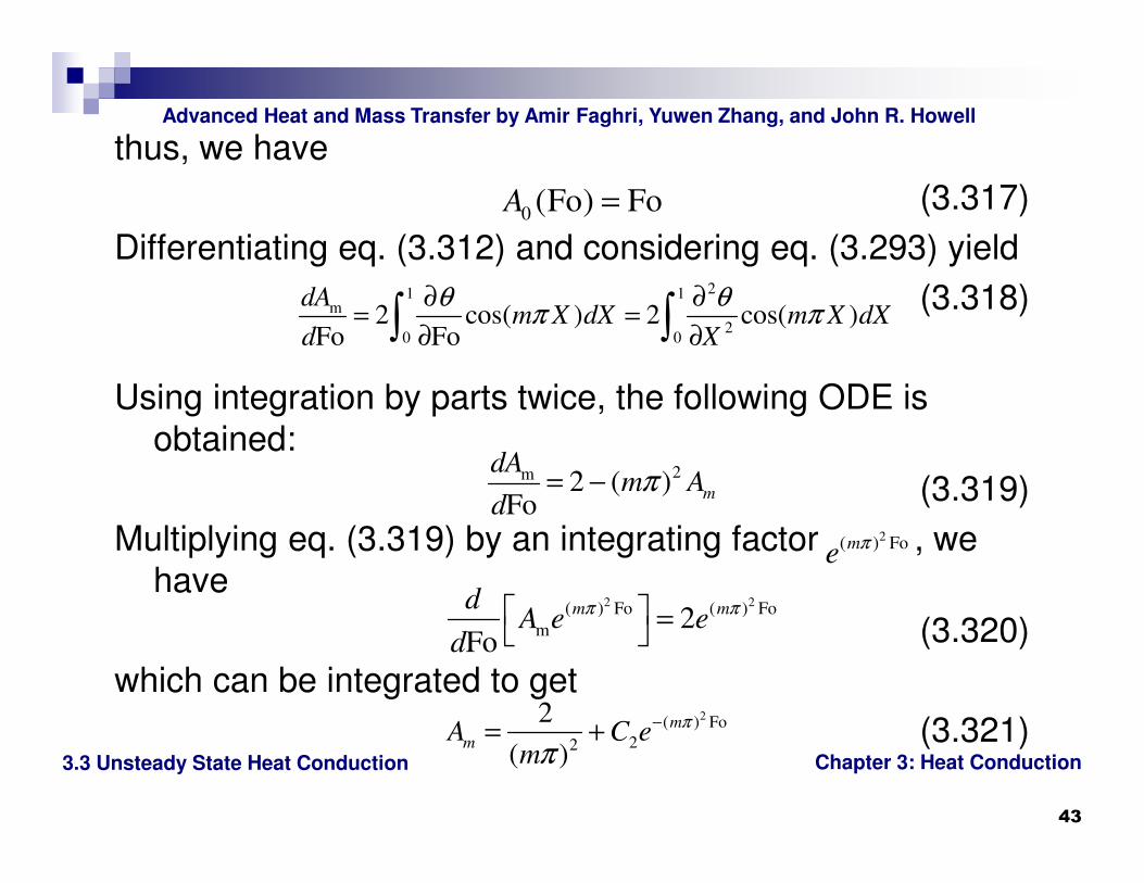
thus, we have
(3.317)
Differentiating eq. (3.312) and considering eq. (3.293) yield
(3.318)
Using integration by parts twice, the following ODE is
obtained:
(3.319)
Multiplying eq. (3.319) by an integrating factor , we
have
(3.320)
which can be integrated to get
(3.321)
0 (Fo) FoA =
21 1m
20 0
2 cos( ) 2 cos( )Fo Fo
dAm X dX m X dX
d X
θ θπ π
∂ ∂= =
∂ ∂∫ ∫
2m 2 ( )Fo
m
dAm A
dπ= −
2( ) Fome
π
2 2( ) Fo ( ) Fo
m 2Fo
m mdA e e
d
π π =
2( ) Fo
22
2
( )
m
mA C em
π
π−= +
Chapter 3: Heat Conduction
Advanced Heat and Mass Transfer by Amir Faghri, Yuwen Zhang, and John R. Howell
3.3 Unsteady State Heat Conduction
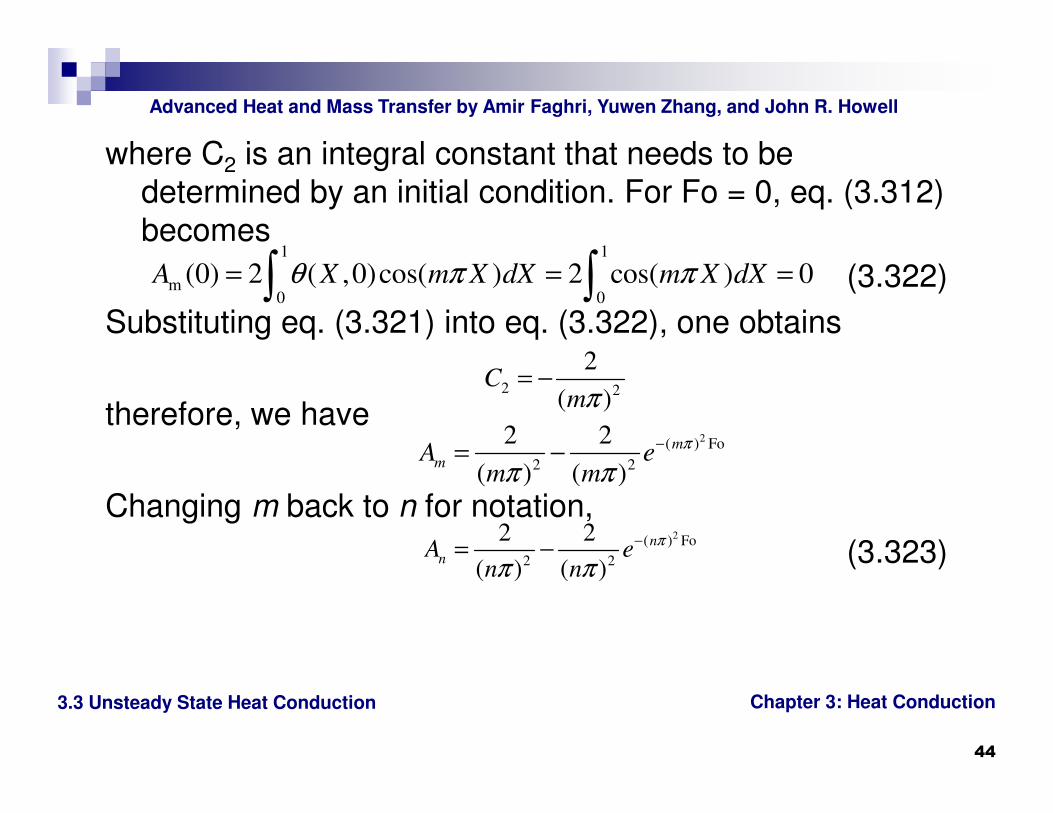
44
where C2 is an integral constant that needs to be
determined by an initial condition. For Fo = 0, eq. (3.312)
becomes
(3.322)
Substituting eq. (3.321) into eq. (3.322), one obtains
therefore, we have
Changing m back to n for notation,
(3.323)
1 1
m0 0
(0) 2 ( ,0)cos( ) 2 cos( ) 0A X m X dX m X dXθ π π= = =∫ ∫
2 2
2
( )C
mπ= −
2( ) Fo
2 2
2 2
( ) ( )
m
mA em m
π
π π−= −
2( ) Fo
2 2
2 2
( ) ( )
n
nA en n
π
π π−= −
Chapter 3: Heat Conduction
Advanced Heat and Mass Transfer by Amir Faghri, Yuwen Zhang, and John R. Howell
3.3 Unsteady State Heat Conduction
45
Substituting eqs. (3.317) and (3.323) into eq. (3.308), the
solution becomes
(3.324)
When the time (Fourier number) becomes large, the last
term on the right-hand side will become zero and the
solution is represented by the first two terms only. To
simplify eq. (3.324), let us assume the solution at large
Fo can be expressed as
(3.325)
which is referred to as asymptotic solution and it must
satisfy eqs. (3.293) – (3.295). Substituting eq. (3.325)
into eqs. (3.293) – (3.295), we have
(3.326)
( ) ( ) 2( ) Fo
2 2 2 2
1 1
cos cos2 2( ,Fo) Fo+ n
n n
n X n XX e
n n
ππ πθ
π π
∞ ∞−
= =
= −∑ ∑
( ,Fo) Fo+ ( )X f Xθ =
( ) 1f X′′ =
Chapter 3: Heat Conduction
Advanced Heat and Mass Transfer by Amir Faghri, Yuwen Zhang, and John R. Howell
3.3 Unsteady State Heat Conduction
46
(3.327)
Integrating eq. (3.326) and considering eq. (3.327), we
obtain
(3.328)
where C cannot be determined from eq. (3.327) because
both boundary conditions are for the first order
derivative. To determine C, we can expand f(X) defined
in eq. (3.328) into cosine Fourier series, i.e.
(3.329)
After determining a0 and an, and considering the f(X) is
identical to the second term on the right-hand side of eq.
(3.324), we have
(3.330)
(0) 1, (1) 0f f′ ′= − =
2
( )2
Xf X X C= − +
2
0
1
( ) cos( )2
n
n
Xf X X C a a n Xπ
∞
=
= − + = +∑
( )2
2 2
1
cos1 2
2 3n
n XXX
n
π
π
∞
=
− + = ∑
Chapter 3: Heat Conduction
Advanced Heat and Mass Transfer by Amir Faghri, Yuwen Zhang, and John R. Howell
3.3 Unsteady State Heat Conduction
47
Substituting eq. (3.330) into eq. (3.324), the final solution
becomes
(3.331)( ) 2
2( ) Fo
2 2
1
cos1 2( ,Fo) Fo+
2 3
n
n
n XXX X e
n
ππθ
π
∞−
=
= − + − ∑
Chapter 3: Heat Conduction
Advanced Heat and Mass Transfer by Amir Faghri, Yuwen Zhang, and John R. Howell
3.3 Unsteady State Heat Conduction
48
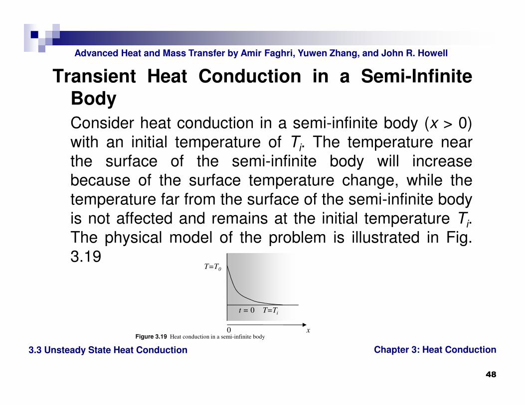
Transient Heat Conduction in a Semi-Infinite
Body
Consider heat conduction in a semi-infinite body (x > 0)
with an initial temperature of Ti. The temperature near
the surface of the semi-infinite body will increase
because of the surface temperature change, while the
temperature far from the surface of the semi-infinite body
is not affected and remains at the initial temperature Ti.
The physical model of the problem is illustrated in Fig.
3.19
T=Ti
Figure 3.19 Heat conduction in a semi-infinite body0 x
T=T0
t = 0

Chapter 3: Heat Conduction
Advanced Heat and Mass Transfer by Amir Faghri, Yuwen Zhang, and John R. Howell
3.3 Unsteady State Heat Conduction
49
The governing equation of the heat conduction problem
and the corresponding initial and boundary conditions
are:
(3.332)
(3.333)
(3.334)
(3.335)
which can be solved by using the method of separation of
variables or integral approximate solution.
Defining the following dimensionless variables
(3.336)
where L is a characteristic length.
2
2
( ) 1 ( )0 0
T x t T x tx t
x tα
∂ , ∂ ,= > , >
∂ ∂
0( ) 0 0T x t T x t, = = , >
( ) 0iT x t T x t, = → ∞, >
( ) 0 0i
T x t T x t, = > , =
0
2
0
, , Foi
T T x tX
T T L L
αθ
−= = =
−
Chapter 3: Heat Conduction
Advanced Heat and Mass Transfer by Amir Faghri, Yuwen Zhang, and John R. Howell
3.3 Unsteady State Heat Conduction
50
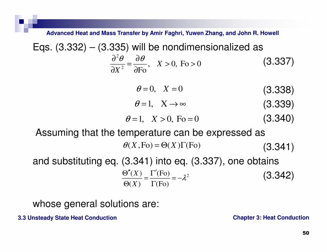
Eqs. (3.332) – (3.335) will be nondimensionalized as
(3.337)
(3.338)
(3.339)
(3.340)
Assuming that the temperature can be expressed as
(3.341)
and substituting eq. (3.341) into eq. (3.337), one obtains
(3.342)
whose general solutions are:
2
2, 0, Fo 0
FoX
X
θ θ∂ ∂= > >
∂ ∂
0, 0Xθ = =
1, Xθ = → ∞
1, 0, Fo 0Xθ = > =
( ,Fo) ( ) (Fo)X Xθ = Θ Γ
2( ) (Fo)
( ) (Fo)
X
Xλ
′′ ′Θ Γ= = −
Θ Γ
Chapter 3: Heat Conduction
Advanced Heat and Mass Transfer by Amir Faghri, Yuwen Zhang, and John R. Howell
3.3 Unsteady State Heat Conduction
51
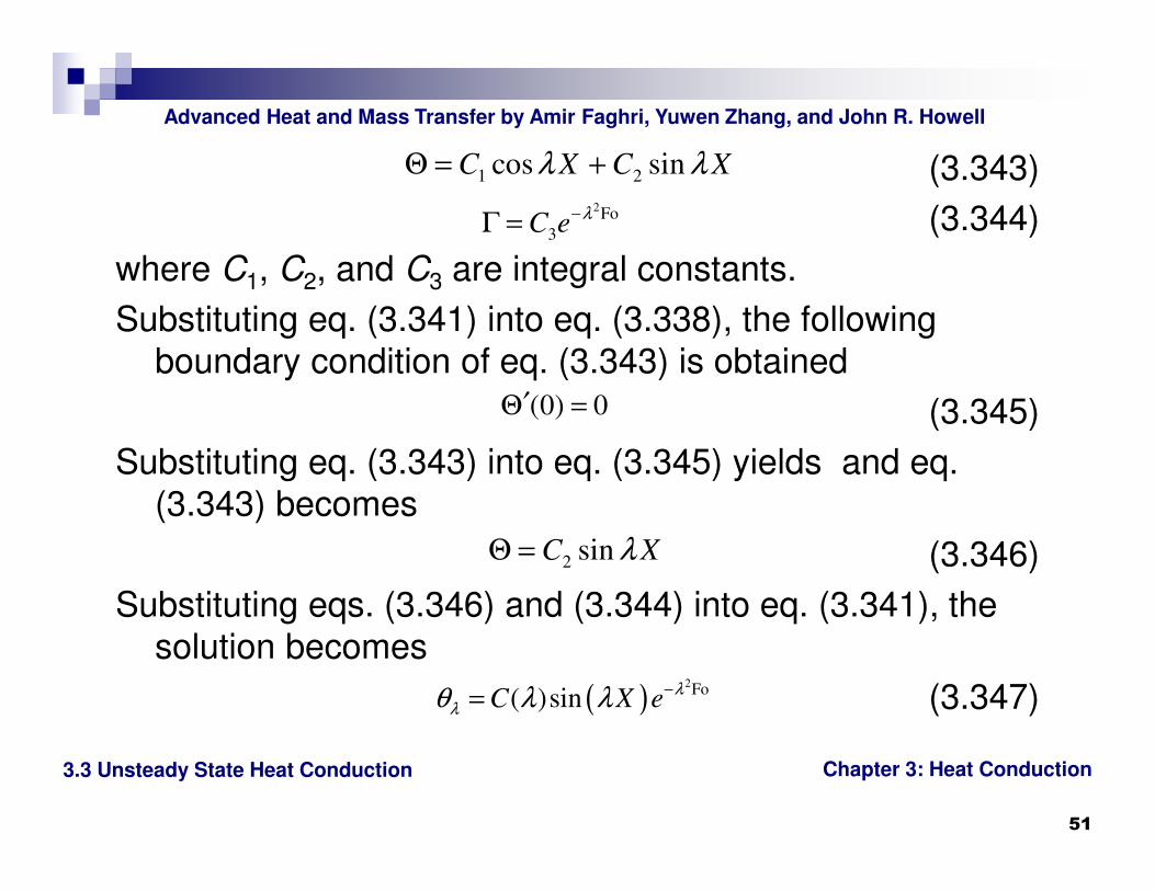
(3.343)
(3.344)
where C1, C2, and C3 are integral constants.
Substituting eq. (3.341) into eq. (3.338), the following
boundary condition of eq. (3.343) is obtained
(3.345)
Substituting eq. (3.343) into eq. (3.345) yields and eq.
(3.343) becomes
(3.346)
Substituting eqs. (3.346) and (3.344) into eq. (3.341), the
solution becomes
(3.347)
1 2cos sinC X C Xλ λΘ = +2Fo
3C e λ−Γ =
(0) 0′Θ =
2 sinC XλΘ =
( )2Fo
( )sinC X eλ
λθ λ λ −=
Chapter 3: Heat Conduction
Advanced Heat and Mass Transfer by Amir Faghri, Yuwen Zhang, and John R. Howell
3.3 Unsteady State Heat Conduction
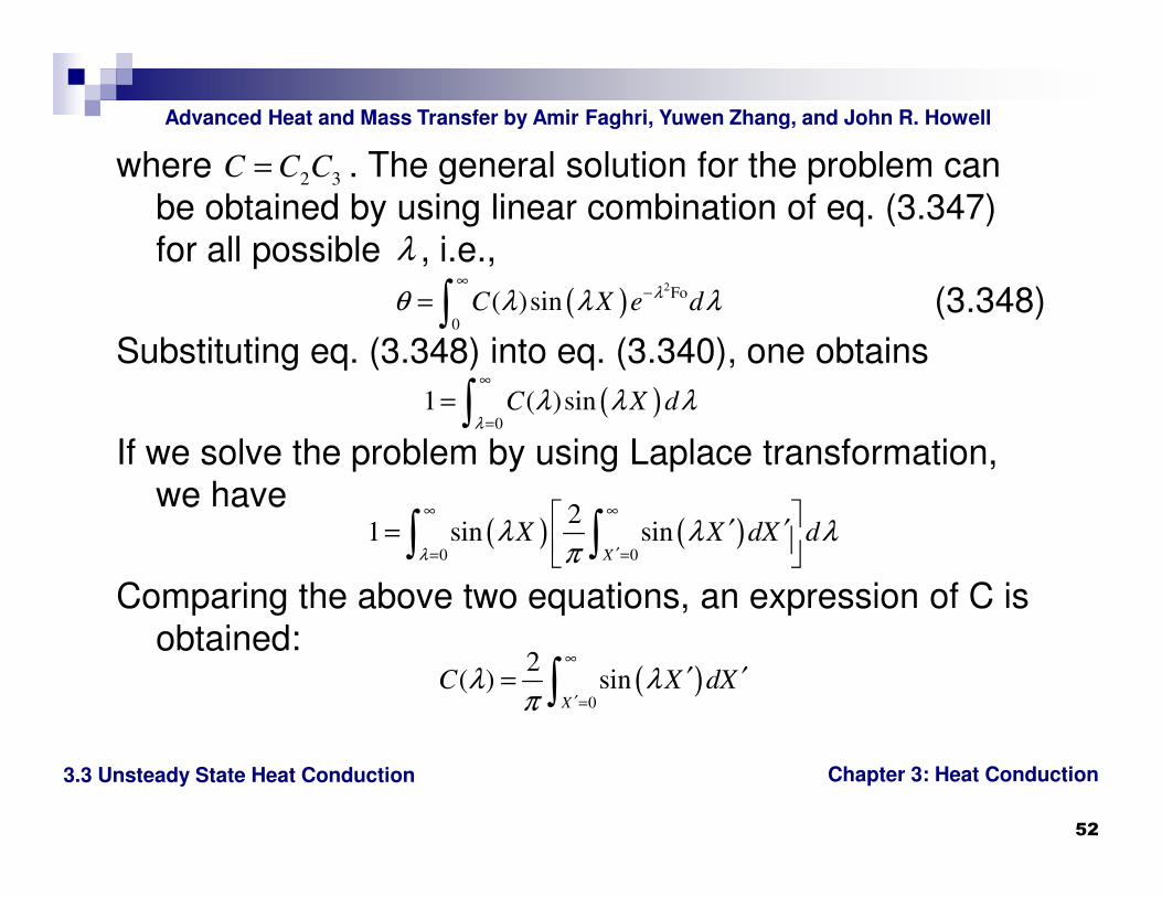
52
where . The general solution for the problem can
be obtained by using linear combination of eq. (3.347)
for all possible , i.e.,
(3.348)
Substituting eq. (3.348) into eq. (3.340), one obtains
If we solve the problem by using Laplace transformation,
we have
Comparing the above two equations, an expression of C is
obtained:
2 3C C C=
λ
( )2Fo
0
( )sinC X e dλθ λ λ λ
∞−= ∫
( )0
1 ( )sinC X dλ
λ λ λ∞
== ∫
( ) ( )0 0
21 sin sin
X
X X dX dλ
λ λ λπ
∞ ∞
′= =
′ ′= ∫ ∫
( )0
2( ) sin
X
C X dXλ λπ
∞
′=
′ ′= ∫
Chapter 3: Heat Conduction
Advanced Heat and Mass Transfer by Amir Faghri, Yuwen Zhang, and John R. Howell
3.3 Unsteady State Heat Conduction
53
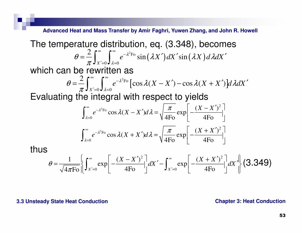
The temperature distribution, eq. (3.348), becomes
which can be rewritten as
Evaluating the integral with respect to yields
thus
(3.349)
( ) ( )2Fo
0 0
2sin sin
X
e X dX X d dXλ
λθ λ λ λ
π
∞ ∞−
′= =
′ ′ ′= ∫ ∫
[ ]2Fo
0 0
2cos ( ) cos ( )
X
e X X X X d dXλ
λθ λ λ λ
π
∞ ∞−
′= =
′ ′ ′= − − +∫ ∫
22
Fo
0
( )cos ( ) exp
4Fo 4Fo
X Xe X X d
λ
λ
πλ λ
∞−
=
′ −′− = −
∫
22
Fo
0
( )cos ( ) exp
4Fo 4Fo
X Xe X X d
λ
λ
πλ λ
∞−
=
′ +′+ = −
∫
2 2
0 0
1 ( ) ( )exp exp
4Fo 4Fo4 Fo X X
X X X XdX dXθ
π
∞ ∞
′ ′= =
′ ′ − + ′ ′= − − −
∫ ∫
Chapter 3: Heat Conduction
Advanced Heat and Mass Transfer by Amir Faghri, Yuwen Zhang, and John R. Howell
3.3 Unsteady State Heat Conduction
54
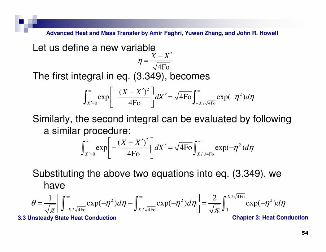
Let us define a new variable
The first integral in eq. (3.349), becomes
Similarly, the second integral can be evaluated by following
a similar procedure:
Substituting the above two equations into eq. (3.349), we
have
4Fo
X Xη
′−=
22
0 / 4Fo
( )exp 4Fo exp( )
4FoX X
X XdX dη η
∞ ∞
′= −
′ −′− = −
∫ ∫
22
0 / 4Fo
( )exp 4Fo exp( )
4FoX X
X XdX dη η
∞ ∞
′=
′ +′− = −
∫ ∫
/ 4Fo2 2 2
/ 4Fo / 4Fo 0
1 2exp( ) exp( ) exp( )
X
X X
d d dθ η η η η η ηπ π
∞ ∞
−
= − − − = − ∫ ∫ ∫
Chapter 3: Heat Conduction
Advanced Heat and Mass Transfer by Amir Faghri, Yuwen Zhang, and John R. Howell
3.3 Unsteady State Heat Conduction
55
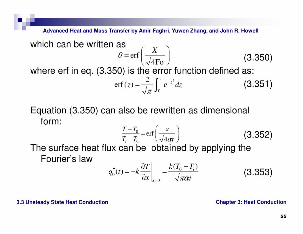
which can be written as
(3.350)
where erf in eq. (3.350) is the error function defined as:
(3.351)
Equation (3.350) can also be rewritten as dimensional
form:
(3.352)
The surface heat flux can be obtained by applying the
Fourier’s law
(3.353)
erf4Fo
Xθ
=
2
0
2erf ( )
zz
z e dzπ
−= ∫
0
0
erf4i
T T x
T T tα
− =
−
00
0
( )( ) i
x
k T TTq t k
x tπα=
−∂′′ = − =
∂
Chapter 3: Heat Conduction
Advanced Heat and Mass Transfer by Amir Faghri, Yuwen Zhang, and John R. Howell
3.3 Unsteady State Heat Conduction
56
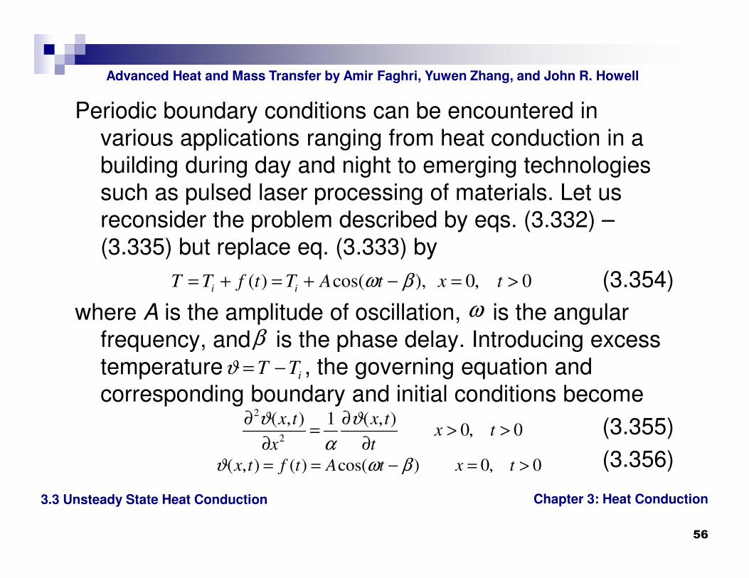
Periodic boundary conditions can be encountered in
various applications ranging from heat conduction in a
building during day and night to emerging technologies
such as pulsed laser processing of materials. Let us
reconsider the problem described by eqs. (3.332) –
(3.335) but replace eq. (3.333) by
(3.354)
where A is the amplitude of oscillation, is the angular
frequency, and is the phase delay. Introducing excess
temperature , the governing equation and
corresponding boundary and initial conditions become
(3.355)
(3.356)
( ) cos( ), 0 0i i
T T f t T A t x tω β= + = + − = , >
ω
β
iT Tϑ = −
2
2
( ) 1 ( )0 0
x t x tx t
x t
ϑ ϑ
α
∂ , ∂ ,= > , >
∂ ∂( ) ( ) cos( ) 0 0x t f t A t x tϑ ω β, = = − = , >
Chapter 3: Heat Conduction
Advanced Heat and Mass Transfer by Amir Faghri, Yuwen Zhang, and John R. Howell
3.3 Unsteady State Heat Conduction
57
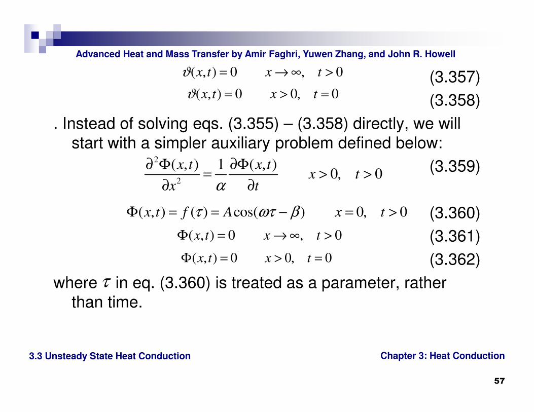
(3.357)
(3.358)
. Instead of solving eqs. (3.355) – (3.358) directly, we will
start with a simpler auxiliary problem defined below:
(3.359)
(3.360)
(3.361)
(3.362)
where in eq. (3.360) is treated as a parameter, rather
than time.
( ) 0 0x t x tϑ , = → ∞, >
( ) 0 0 0x t x tϑ , = > , =
2
2
( ) 1 ( )0 0
x t x tx t
x tα
∂ Φ , ∂Φ ,= > , >
∂ ∂
( ) ( ) cos( ) 0 0x t f A x tτ ωτ βΦ , = = − = , >
( ) 0 0x t x tΦ , = → ∞, >
( ) 0 0 0x t x tΦ , = > , =
τ

Chapter 3: Heat Conduction
Advanced Heat and Mass Transfer by Amir Faghri, Yuwen Zhang, and John R. Howell
3.3 Unsteady State Heat Conduction
58
The Duhamel’s theorem stated that the solution the original
problem is related to the solution of auxiliary problem by
(3.363)
which can rewritten using Leibniz’s rule
(3.364)
The second term on the right hand side is
(3.365)
therefore, eq. (3.364) becomes
(3.366)
0
( , ) ( , , )t
x t x t dt τ
ϑ τ τ τ=
∂= Φ −
∂ ∫
0
( , ) ( , , ) ( , , )t
tx t x t d x t
t ττ
ϑ τ τ τ τ τ=
=
∂= Φ − + Φ −
∂∫
( , , ) ( ,0, ) 0t
x t xτ
τ τ τ=
Φ − = Φ =
0
( , ) ( , , )t
x t x t dtτ
ϑ τ τ τ=
∂= Φ −
∂∫
Chapter 3: Heat Conduction
Advanced Heat and Mass Transfer by Amir Faghri, Yuwen Zhang, and John R. Howell
3.3 Unsteady State Heat Conduction
59
The solution of the auxiliary problem can be expressed as
(3.367)
The partial derivative appearing in eq. (3.366) can be
evaluated as
(3.368)
Substituting eq. (3.368) into eq. (3.366), the solution of the
original problem becomes
(3.369)
2
/ 4
2 ( )( , , ) ( ) 1- erf
4 x t
x fx t f e d
t
η
α
ττ τ η
α π
∞−
Φ = =
∫
2
3/ 2( , , ) ( ) exp
4 ( )4 ( )
x xx t f
t ttτ τ τ
α τπα τ
∂Φ − = −
∂ −−
2
3/ 20
( )( , ) exp
( ) 4 ( )4
tx f xx t d
t tτ
τϑ τ
τ α τπα =
= −
− − ∫
Chapter 3: Heat Conduction
Advanced Heat and Mass Transfer by Amir Faghri, Yuwen Zhang, and John R. Howell
3.3 Unsteady State Heat Conduction
60
Introducing a new independent variable
eq. (3.369) becomes
(3.370)
For the periodic boundary condition specified in eq. (3.356),
we have
(3.371)
which can be rewritten as
(3.372)
4 ( )
x
tξ
α τ=
−
22
2/ 4
2( , ) exp( )
4x t
xx t f t d
αϑ ξ ξ
αξπ
∞ = − −
∫
22
2/ 4
2( , ) cos exp( )
4x t
A xx t t d
αϑ ω β ξ ξ
αξπ
∞ = − − −
∫
22
20
2/ 42
20
2( , ) cos exp( )
4
2 cos exp( )
4
x t
A xx t t d
A xt d
α
ϑ ω β ξ ξαξπ
ω β ξ ξαξπ
∞ = − − −
− − − −
∫
∫

Chapter 3: Heat Conduction
Advanced Heat and Mass Transfer by Amir Faghri, Yuwen Zhang, and John R. Howell
3.3 Unsteady State Heat Conduction
61
Evaluating the first integral on the right hand side of eq.
(3.372) yields
(3.373)
It can be seen that as , the second term will become
zero and the first term represents the steady oscillation.
(3.374)
where represents the amplitude of
oscillation at point x, and in the cosine
function represents the phase delay of oscillation at point
x relative to the oscillation of the surface temperature.
1/ 2 1/ 2
2/ 42
20
( , ) exp cos2 2
2 cos exp( )
4
x t
x t A x t x
A xt d
α
ω ωϑ ω β
α α
ω β ξ ξαξπ
= − − −
− − − −
∫
t → ∞
1/ 2 1/ 2
( , ) exp cos2 2
s x t A x t xω ω
ϑ ω βα α
= − − −
( )1/ 2
exp /(2 )A x ω α −
( )1/ 2
/(2 )x ω α−
Chapter 3: Heat Conduction
Advanced Heat and Mass Transfer by Amir Faghri, Yuwen Zhang, and John R. Howell
3.3 Unsteady State Heat Conduction
62
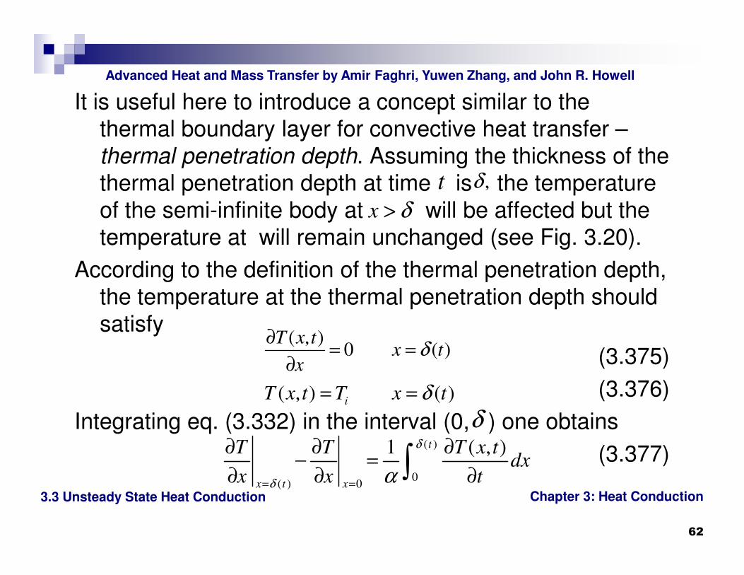
It is useful here to introduce a concept similar to the
thermal boundary layer for convective heat transfer –
thermal penetration depth. Assuming the thickness of the
thermal penetration depth at time is the temperature
of the semi-infinite body at will be affected but the
temperature at will remain unchanged (see Fig. 3.20).
According to the definition of the thermal penetration depth,
the temperature at the thermal penetration depth should
satisfy
(3.375)
(3.376)
Integrating eq. (3.332) in the interval (0, ) one obtains
(3.377)
t δ ,
x δ>
( )0 ( )
T x tx t
xδ
∂ ,= =
∂
( ) ( )iT x t T x tδ, = =
δ( )
0( ) 0
1 ( )t
x t x
T T T x tdx
x x t
δ
δ α= =
∂ ∂ ∂ ,− =
∂ ∂ ∂∫
Chapter 3: Heat Conduction
Advanced Heat and Mass Transfer by Amir Faghri, Yuwen Zhang, and John R. Howell
3.3 Unsteady State Heat Conduction
63
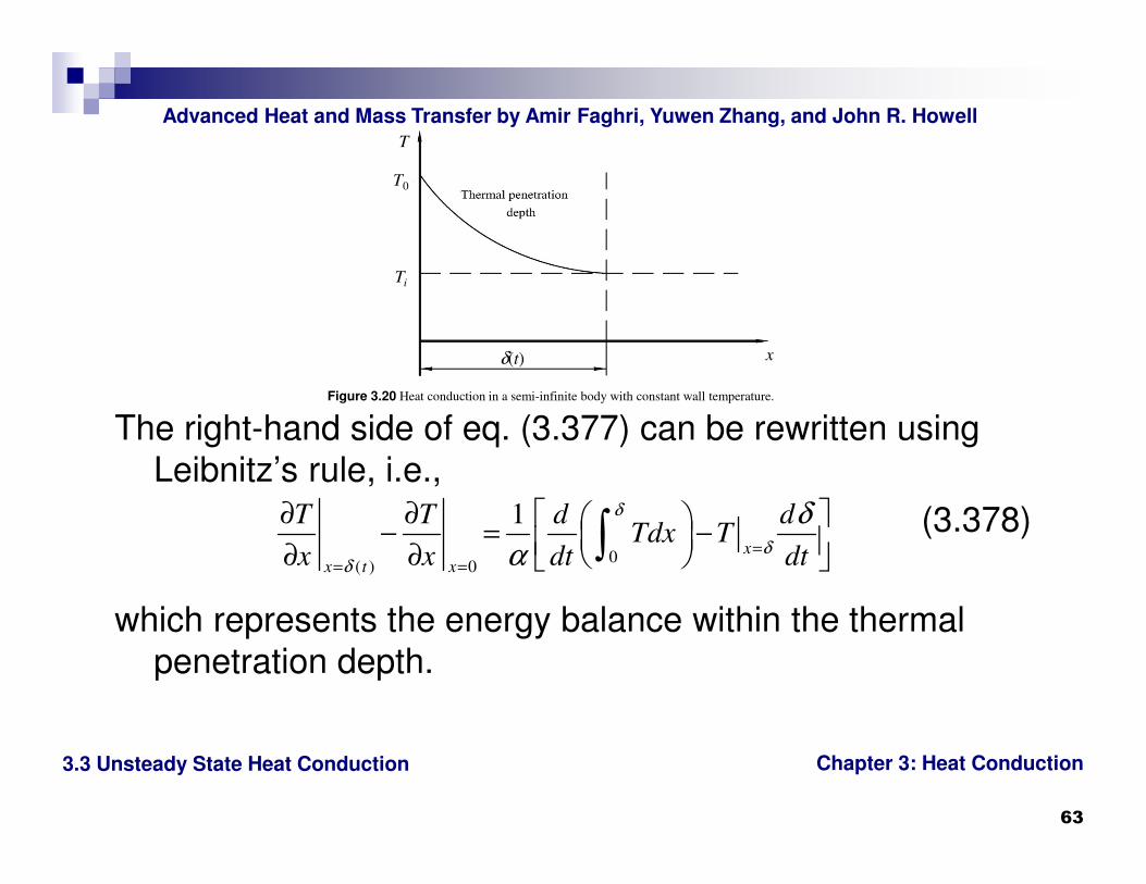
The right-hand side of eq. (3.377) can be rewritten using
Leibnitz’s rule, i.e.,
(3.378)
which represents the energy balance within the thermal
penetration depth.
δ(t)
Ti
T0
T
x
Figure 3.20 Heat conduction in a semi-infinite body with constant wall temperature.
0( ) 0
1x
x t x
T T d dTdx T
x x dt dt
δ
δδ
δ
α == =
∂ ∂ − = − ∂ ∂ ∫
Chapter 3: Heat Conduction
Advanced Heat and Mass Transfer by Amir Faghri, Yuwen Zhang, and John R. Howell
3.3 Unsteady State Heat Conduction
64
Substituting eqs. (3.375) and (3.376) into eq. (3.378) yields
(3.379)
where
(3.380)
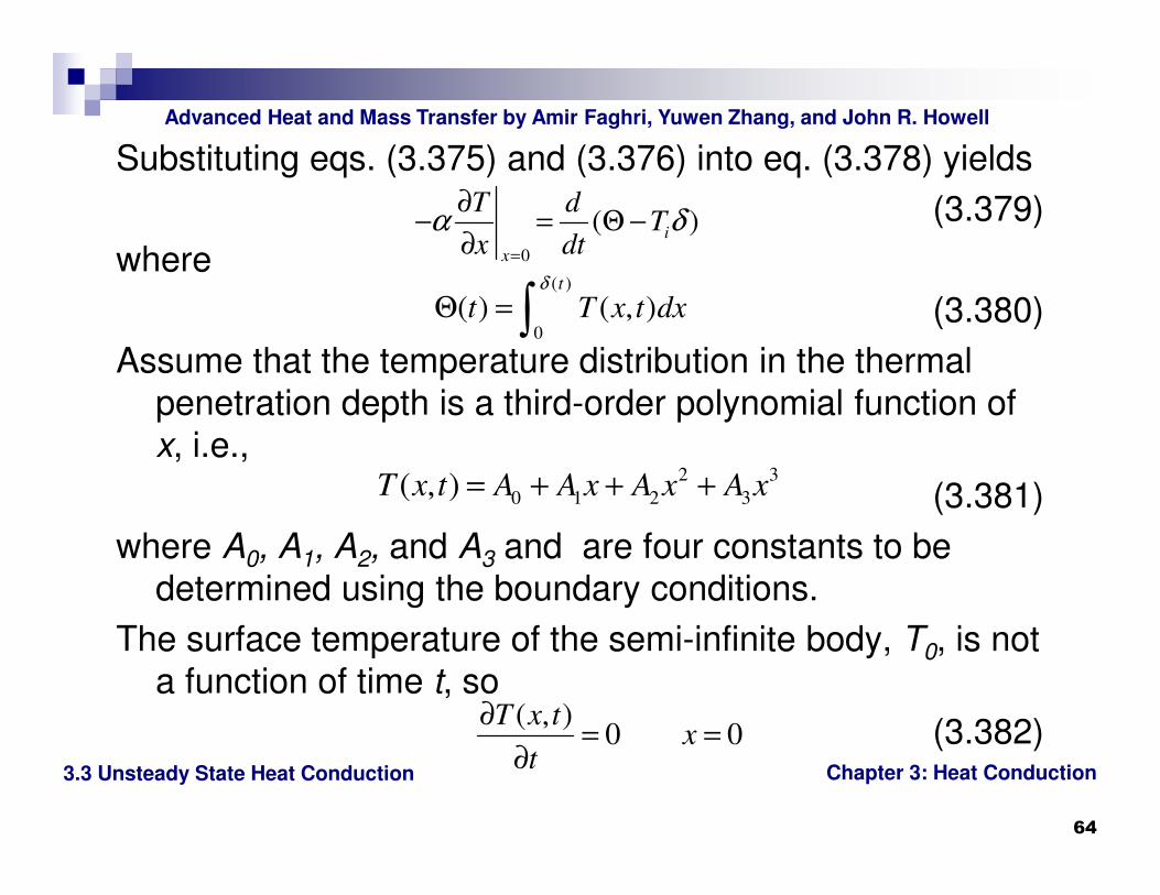
Assume that the temperature distribution in the thermal
penetration depth is a third-order polynomial function of
x, i.e.,
(3.381)
where A0, A1, A2, and A3 and are four constants to be
determined using the boundary conditions.
The surface temperature of the semi-infinite body, T0, is not
a function of time t, so
(3.382)
0
( )i
x
T dT
x dtα δ
=
∂− = Θ −
∂( )
0
( ) ( )t
t T x t dxδ
Θ = ,∫
2 3
0 1 2 3( )T x t A A x A x A x, = + + +
( )0 0
T x tx
t
∂ ,= =
∂
Chapter 3: Heat Conduction
Advanced Heat and Mass Transfer by Amir Faghri, Yuwen Zhang, and John R. Howell
3.3 Unsteady State Heat Conduction
65
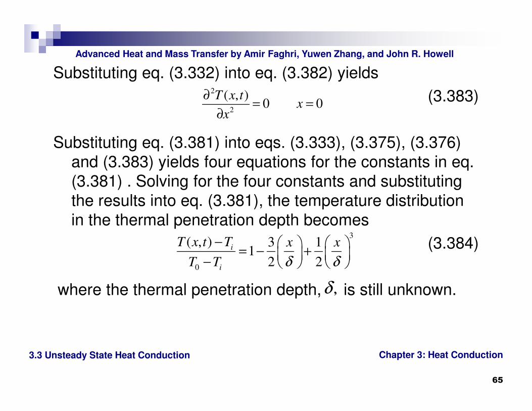
Substituting eq. (3.332) into eq. (3.382) yields
(3.383)
Substituting eq. (3.381) into eqs. (3.333), (3.375), (3.376)
and (3.383) yields four equations for the constants in eq.
(3.381) . Solving for the four constants and substituting
the results into eq. (3.381), the temperature distribution
in the thermal penetration depth becomes
(3.384)
where the thermal penetration depth, is still unknown.
2
2
( )0 0
T x tx
x
∂ ,= =
∂
3
0
( ) 3 11
2 2
i
i
T x t T x x
T T δ δ
, − = − +
−
δ ,

Chapter 3: Heat Conduction
Advanced Heat and Mass Transfer by Amir Faghri, Yuwen Zhang, and John R. Howell
3.3 Unsteady State Heat Conduction
66
Substituting eq. (3.384) into eq. (3.379), an ordinary
differential equation for is obtained:
(3.385)
Since the thermal penetration depth equals zero at the
beginning of the heat conduction, eq. (3.385) is subject
to the following initial condition:
(3.386)
The solution of eqs. (3.385) and (3.386) is
(3.387)
which is consistent with the result of scale analysis,
4 0d
tdt
δα δ= >
δ
0 0tδ = =
8 tδ α=
tδ α∼

Chapter 3: Heat Conduction
Advanced Heat and Mass Transfer by Amir Faghri, Yuwen Zhang, and John R. Howell
3.3 Unsteady State Heat Conduction
67
Consider transient heat conduction in a rectangular bar
with dimensions of 2L1×2L2 and an initial temperature of
Ti (see Fig. 3.21). At time t = 0, the rectangular bar is
immersed into a fluid with temperature T∞.
3.3.2 Multidimensional Transient
Heat Conduction Systems
3.3.2 Multidimensional Transient
Heat Conduction Systems
Figure 3.21 Two-dimensional transient heat conduction
–
L1
L1 x
h1,T∞
y
0
h1,T∞
h2,T∞L2
h2,T∞-L2
Chapter 3: Heat Conduction
Advanced Heat and Mass Transfer by Amir Faghri, Yuwen Zhang, and John R. Howell
3.3 Unsteady State Heat Conduction
68
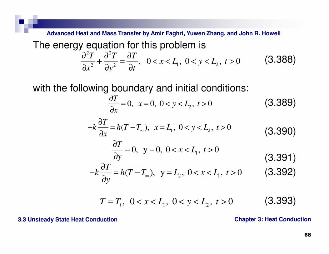
The energy equation for this problem is
(3.388)
with the following boundary and initial conditions:
(3.389)
(3.390)
(3.391)
(3.392)
(3.393)
2 2
1 22 2, 0 , 0 , 0
T T Tx L y L t
x y t
∂ ∂ ∂+ = < < < < >
∂ ∂ ∂
20, 0, 0 , 0T
x y L tx
∂= = < < >
∂
1 2( ), , 0 , 0T
k h T T x L y L tx
∞
∂− = − = < < >
∂
10, y 0, 0 , 0T
x L ty
∂= = < < >
∂
2 1( ), y , 0 , 0T
k h T T L x L ty
∞
∂− = − = < < >
∂
1 2, 0 , 0 , 0iT T x L y L t= < < < < >
Chapter 3: Heat Conduction
Advanced Heat and Mass Transfer by Amir Faghri, Yuwen Zhang, and John R. Howell
3.3 Unsteady State Heat Conduction
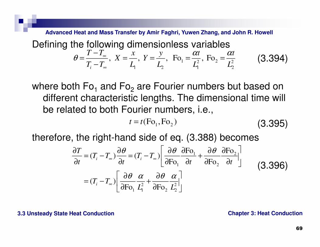
69
Defining the following dimensionless variables
(3.394)
where both Fo1 and Fo2 are Fourier numbers but based on
different characteristic lengths. The dimensional time will
be related to both Fourier numbers, i.e.,
(3.395)
therefore, the right-hand side of eq. (3.388) becomes
(3.396)
1 22 2
1 2 1 2
, , , Fo , Foi
T T x y t tX Y
T T L L L L
α αθ ∞
∞
−= = = = =
−
1 2(Fo ,Fo )t t=
1 2
1 2
2 2
1 1 2 2
Fo Fo( ) ( )
Fo Fo
( )Fo Fo
i i
i
TT T T T
t t t t
T TL L
θ θ θ
θ α θ α
∞ ∞
∞
∂ ∂∂ ∂ ∂ ∂= − = − +
∂ ∂ ∂ ∂ ∂ ∂
∂ ∂= − +
∂ ∂

Chapter 3: Heat Conduction
Advanced Heat and Mass Transfer by Amir Faghri, Yuwen Zhang, and John R. Howell
3.3 Unsteady State Heat Conduction
70
Nondimensionalizing the left-hand side of eq. (3.388) and
considering eq. (3.396), the dimensionless energy
equation of the problem becomes
(3.397)
The boundary and initial conditions, eqs. (3.389) – (3.393)
are nondimensionalized as
(3.398)
(3.399)
(3.400)
(3.401)
2 22 2
1 1
2 2
2 1 2 2Fo Fo
L L
X L Y L
θ θ θ θ ∂ ∂ ∂ ∂+ = +
∂ ∂ ∂ ∂
1 20, X 0, 0 1, Fo 0, Fo 0YX
θ∂= = < < > >
∂
1 1 2Bi , X 1, 0 1, Fo 0, Fo 0YX
θθ
∂− = = < < > >
∂
1 20, Y 0, 0 1, Fo 0, Fo 0XY
θ∂= = < < > >
∂
2 1 2Bi , 1, 0 1, Fo 0, Fo 0Y XY
θθ
∂− = = < < > >
∂

Chapter 3: Heat Conduction
Advanced Heat and Mass Transfer by Amir Faghri, Yuwen Zhang, and John R. Howell
3.3 Unsteady State Heat Conduction
71
(3.402)
where
(3.403)
are Bio numbers for different surfaces.
The idea of product solution is that the solution of the two-
dimensional problem can be expressed as the product of
two one-dimensional problem, i.e.,
(3.404)
where is the solution of the following problem
(3.405)
(3.406)
1 21, 0 1, 0 1, Fo Fo 0X Yθ = < < < < = =
1 1 2 21 2Bi , Bi
h L h L
k k= =
1 2( ,Fo ) ( ,Fo )X Yθ ϕ ψ=
ϕ2
2
1FoX
ϕ ϕ∂ ∂=
∂ ∂
10, X 0, Fo 0X
ϕ∂= = >
∂
Chapter 3: Heat Conduction
Advanced Heat and Mass Transfer by Amir Faghri, Yuwen Zhang, and John R. Howell
3.3 Unsteady State Heat Conduction
72
(3.407)
(3.408)
and satisfies
(3.409)
(3.410)
(3.411)
(3.412)
It can be demonstrated that eqs. (3.397) – (3.402) can be
satisfied by eq. (3.404) if and are solutions of eqs.
(3.405) – (3.408) and (3.409) – (3.4120), respectively.
The solution of eqs. (3.405) – (3.408) is:
(3.413)
1 1Bi , X 1, Fo 0X
ϕϕ
∂− = = >
∂
11, 0 1, Fo 0Xϕ = < < =
ψ 2
2
2FoY
ψ ψ∂ ∂=
∂ ∂
20, 0, Fo 0YY
ψ∂= = >
∂
2 2Bi , 1, Fo 0YY
ψψ
∂− = = >
∂
21, 0 1, Fo 0Yψ = < < =
ϕ ψ
( )2
1Fo
1
4sincos
2 sin 2nn
n
n nn
X eλλ
ϕ λλ λ
∞−
=
=+∑

Chapter 3: Heat Conduction
Advanced Heat and Mass Transfer by Amir Faghri, Yuwen Zhang, and John R. Howell
3.3 Unsteady State Heat Conduction
73
Where
(3.414)
and the solution of eqs. (3.409) – (3.412) is
(3.415)
where
(3.416)
Substituting eqs. (3.413) and (3.415) into eq. (3.404), the
solution of the two-dimensional problem is obtained.
(3.417)
1
cotBi
n
n
λλ=
( )2
2Fo
1
4sincos
2 sin 2mn
m
m mm
Y eνν
ψ νν ν
∞−
=
=+∑
2
cotBi
m
m
νν=
( ) ( ) 2 21 2( Fo Fo )
1 1
16sin sin cos cos
(2 sin 2 )(2 sin 2 )n mn m n m
n n m mn m
X Ye
λ νλ ν λ νθ
λ λ ν ν
∞ ∞− +
= =
=+ +∑∑