TRANSACTIONS OF INTELLIGENT … OF INTELLIGENT TRANSPORTATION SYSTEMS, VOL. 12, NO. 4, DECEMBER 2011 1 Probabilistic Rail Vehicle Localization with Eddy Current Sensors in Topological

TRANSACTIONS OF INTELLIGENT TRANSPORTATION SYSTEMS, VOL. 12, NO. 4, DECEMBER 2011 1

Probabilistic Rail Vehicle Localization with EddyCurrent Sensors in Topological MapsStefan Hensel, Student Member, IEEE, Carsten Hasberg, Student Member, IEEE,

and Christoph Stiller, Senior Member, IEEE

Abstract—The precise localization of rail vehicles is fundamen-tal for the development and employment of more efficient traincontrol systems in security, logistics and disposition applications.Current research in train navigation systems tries to solve thetask with an increasing number of onboard sensors or addi-tional infrastructure installations in combination with satellitenavigation (GNSS). Both approaches are cost intensive and relyon undisturbed satellite signals, commonly not given in railroadapplications. In contrast, we describe a novel, single sensor,onboard localization system in this contribution, based on a newlydeveloped eddy current sensor (ECS). We outline an onboardlocalization system within a probabilistic framework, with specialattention on signal processing for speed estimation and patternrecognition. In particular, we employ Bayesian methods such ashidden Markov models for turnout detection and classificationand, in a final step, sequential Monte Carlo sampling to combinethe extracted information in a topological map to obtain a reliableposition estimate.

Index Terms—Train Localization, Eddy Current Sensor, Hid-den Markov Models (HMM), Sequential Monte Carlo (SMC).

I. INTRODUCTION

TRAIN localization systems nowadays operate with ahigh amount of track side infrastructure installations.

Future train operating systems, e.g. the European Train ControlSystem (ETCS) on level three [1], are based on an onboardlocalization of rail vehicles to enable more efficient dispositiontechniques such as moving block. Therefore, current researchfocuses on reliable onboard train localization systems. In-spired by localization techniques in air and automotive traffic,the commonly chosen system architecture combines onboardspeed measurement with global navigation satellite systems(GNSS), commonly GPS, to estimate a reliable position in-formation [2]. One drawback of this approach is the relativelylow accuracy of inductive odometrial measurements and theGNSS reliability, given that tracks contain tunnels and roofedstation halls and are often situated either in urban areas,forests or valleys with dense vegetation and high buildings.Hence, the reliability of the obtained solution is insufficient

Manuscript received March 1, 2010; revised August 26, 2010, April 13,2011, and June 22, 2011; Date of publication July 29, 2011. This workwas supported in part by the German Federal Ministry of Economics andTechnology. The Associate Editor for this paper was M. Brackstone.

S. Hensel, C. Hasberg and C. Stiller are with the Institute ofMeasurement and Control Systems, Karlsruhe Institute of Technology(KIT),76131 Karlsruhe, Germany, e-mail: {carsten.hasberg, stefan.hensel,christoph.stiller}@kit.edu.

Color versions of one or more of the figures in this paper are availableonline at http://ieeexplore.ieee.org.

Digital Object Identifier 10.1109/TITS.2011.2161291

for the requested security and technical standards. Currentdisposition methods such as ETCS on level two try to improveaccuracy with additional infrastructure installations to gain re-calibration points, which leads to high track maintenance costs.

Eddy current sensors (ECS) are commonly used for the mea-surement of inhomogeneities within ferromagnetic materials(e.g. see [3]). Based on this principle, we developed a sensorsystem capable of precise non-contact and slipless speedmeasurement in rail vehicles [4], [5]. Besides the increasein odometrial measurements the sensor additionally allowsthe detection and classification of turnouts. In contrast tovision based systems for track and turnout recognition [6], theECS working principle is robust against weather influencesand day time. The sensor outperforms accelerometer basedsystems as [7], [8] with the possibility to detect turnouts passedunbending and to classify individual turnouts.

Rail networks naturally possess a large amount of turnouts,e.g. the German rail network has a total length of approx.38000 km containing about 72000 turnouts. We propose touse these as beacons that are intrinsically distributed accordingto the need of local precision, i.e. lots of turnouts withinstations that contain a lot of parallel tracks for a landmarkbased localization.

The sensor information is one-dimensional and thereforesuited to be employed with topological maps. These are, incontrast to precise metric maps, easy to obtain or can easily becreated by any person that knows the track. Localization withtopological maps is commonly researched in indoor roboticsand examples can be found in [9] or [10]. We illustratehow a combination of robust velocity estimation and reliableturnout detection are sufficient for track specific onboard trainlocalization with ECS rendering other relative and absolutepositioning systems obsolete.

For this purpose we consider and setup the complete local-ization system, which can roughly be subdivided into threeparts. Speed estimation, the recognition of turnouts and thefinal information fusion within a map. To cope with the re-quirements of the system such as heavy duty conditions of railvehicles, different vehicle types, independent noise sources,very large rail networks, and changes in rail infrastructure, weemploy probabilistic methods. The advantages of a stochasticconcept are shown in many robotics [11], tracking [12] andmachine learning [13] applications. The Bayesian frameworkwe employ for turnout extraction and map based localizationis intuitive, robust, and easy augmentable to incorporate ad-ditional sensors. With this our system can be employed as astandalone solution on side tracks or in combination with other


onboard sensor systems for safety applications in ETCS levelthree. Nonetheless, in this contribution we try to emphasizethe individual capability of our localization system.

The remainder of the paper is organized as follows: Sec-tion II will introduce the eddy current sensor system and itsapplication to speed estimation. We propose a novel methodthat alleviates acceleration influences to significantly improvethe velocity estimate quality based on cross-correlation of thesignals, especially when driving in low speed. Recognitionof turnouts with hidden Markov models is subject of Sec-tion III. It is shown how probabilistic models can be employedto detect and continuously extract turnouts. Afterwards, theclassification of the detected samples is analyzed with respectto signal preprocessing, parameter adaptation and model se-lection. Velocity and turnout information must be combinedin a most optimal way within the map, which is subject ofSection IV. We resolve ambiguous position hypotheses, thatare represented by an a posteriori probability density function,with sequential Monte Carlo (SMC) methods. This allowshandling uncertainties in track association that occur whilepassing turnouts or due to misclassifications. The final Sectiongives a summary and conclusions of the localization conceptas well as possible augmentations.

II. EDDY CURRENT SENSOR SYSTEM (ECS)

A. Sensor setup

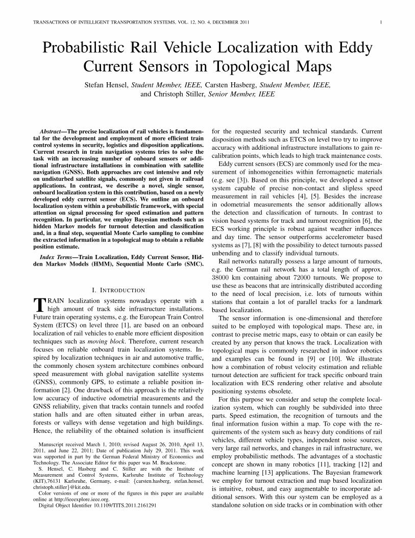
Eddy current sensors are commonly used to detect inhomo-geneities in the magnetic resistance of ferromagnetic materials(e.g. see [3]). This basic approach has been further developedand adapted to possible applications on railway vehicles.These include speed measurement and pattern recognition.For correlation of two signals the eddy current sensor systemconsists of two identical sensor devices, each built up with atransceiver coil and two pick up coils. Both sensors are placedsequentially within a housing, mounted approximately 10 cmabove the rail head. Figure 1(a) displays the principle of asingle sensor unit: The transmitter coil E excites a magneticfield HE, that induces eddy currents in metallic materials likethe rail. The eddy currents induce an antipode magnetic fieldHEC, that generates the voltage uP1(t) and uP2(t) within thepick-up coils P1 and P2 respectively. By interconnecting themdifferentially, the output signal s(t) = uP1(t) − uP2(t) is ameasure for rail inhomogeneities. These mainly result fromrail clamps, turnouts and other irregularities, e.g. cracks orsignal cables (for details see [4]). The signals s1(t) and s2(t)represent a stochastic process. Clamps produce a stationaryprocess for rail vehicles driving on open tracks with constantvelocity. Turnouts, cables, and metallic clutter represent non-stationary signal components, whereas both parts are superim-posed by a noise process that can be regarded as zero meanwhite Gaussian noise. The overall signal comprises a highsignal-to-noise ratio (SNR), given that preprocessing low passfilters are installed in the sensor hardware [14].

B. Velocity estimation

The described working principle is, in contrast to visionbased systems or doppler radar sensors, widely unsusceptible

to environmental perturbations and, because of the differentialsetup, robust against systematic influences. These propertiesare highly desirable for a reliable speed measurement underrough railway conditions. Velocity estimation can commonlybe achieved via cross-correlation of the two sensor signalss1(t) and s2(t), that are idealized depicted in Figure 1(b). Firstapproaches, intended and optimized for hardware realization,apply a closed loop correlator (CLC) assuming a known sensordistance l and a measured time difference ∆t (for detailssee [4]) and [15].

HE H

EC

(a)

S1S2

signal s (t)1

signal s (t)2

(b)

Fig. 1. (a) Single ECS sensor S1 (b) Example signal of ECS (two sensors)s(t) when crossing a rail clamp.

The presented approaches rely on the assumption of astationary stochastic process, which holds for constant velocitywithin the cross-correlation interval. Whereas this assumptionis correct in most situations, it is heavily violated in lowspeed manoeuvres, where large changes in the relative velocitymay occur. This is unfortunately the case in areas of interest,i.e. within stations, where most turnouts are present. The needof a precise spatial signal s(x) for pattern recognition (seeSection III) makes it necessary to apply a velocity estimation,that can cope with these situations. Therefore, we augmentthe common cross correlation analysis by a correlation basedestimation of the current train acceleration. With this, thesignal can be resampled to eliminate correlation windowaveraging effects on an accurate velocity estimate.

The basic idea is to find the time shift ∆t of the signalss1(t) and s2(t), which corresponds to the maximization ofthe cross correlation according to

∆t = arg maxτ

(E {s1(t− τ) · s2(t)}). (1)

We assume a constant acceleration a in a signal of equallength before and after resampling. With an average velocityv0 within the interval TM , the traveled distance dTM

becomes

dTM=

∫ TM

0

v(t) dt =

∫ TM

0

[v0 + at] dt = v0TM +1

2aT 2

M ,

(2)and using signal length equality

dTM= vmN Ts = dTM

= v0N Ts +1

2a(N Ts)

2, (3)

for a discrete sequence of length N and sampling time Ts.


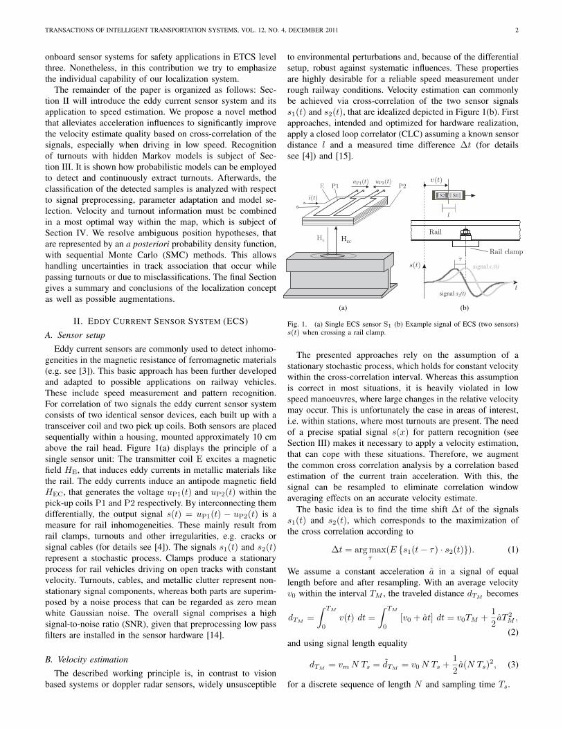
Fig. 2. Cross correlation coefficients plotted against warping factor κ using a 4s window. By varying κ, one can determine κmax that locally maximizescorrelation coefficients. The right figure displays two example coefficients as functions of κ (indicated by the corresponding lines in the left figure).

The association of an original sample no to the resampledoutput sample ni is expressed with (3) and the auxiliaryvariable

ζ :=v0

a · Ts, ζ ∈ (−∞,−N ] ∪ [0,∞), (4)

which results in

ni = −ζ + ζ

√1 +

2noζ

+N · noζ2

. (5)

A more practicable domain is obtained by reparametrization of(5) with a warping factor κ. Under consideration of extremevalues ( [16]) it follows

κ :=4 ∆n

N=

N

2ζ +N, κ ∈ [−1, 1]. (6)

This gives κ a limited range of values with κ ∈ [−1, 1]. Forthe determination of a and v0, ζ is replaced in (6) with

ζ =1− κ2 κ

N. (7)

Thus, the signal resampling for the purpose of maximizingthe cross correlation coefficient is characterized by κ, thatdescribes the signal straining. Figure 2 shows the influenceof κ for the cross correlation quality, and its applicabilityfor acceleration estimates. After resampling, the correlationmaximum is determined with parabolic approximation forsubsample accuracy. The average speed v(t) and accelerationa(t) within a given interval is calculated with

v(t) =l

∆t, a(t) =

2κ · v(t)

L · Ts, (8)

where L is the number of samples within the correlationintegral and TS the sampling time. The estimates of v(t)are subsequently interpreted as observations and merged in aKalman Filter (see [17], [12]) with constant acceleration modelto track the final velocity estimate vest(t). In contrary to a CLCthis approach allows speed estimates down to zero velocity.The additional knowledge of the Kalman Filter accelerationestimate aest(t) is used for validation of the calculated a(t).

Further details on error propagation and results for the velocityestimation are outlined in [16].

The high accuracy of this method allows for subsequentvelocity integration to determine the covered distance insufficient quality, which is first pre-requisite to solve anylocalization problem and calculation of spatial signals s(x),with x =

∫ T0vest(t)dt as covered distance in time T .

III. PATTERN RECOGNITION WITH HMM’S

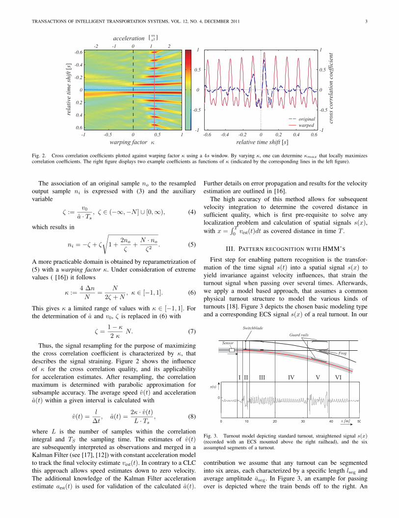
First step for enabling pattern recognition is the transfor-mation of the time signal s(t) into a spatial signal s(x) toyield invariance against velocity influences, that strain theturnout signal when passing over several times. Afterwards,we apply a model based approach, that assumes a commonphysical turnout structure to model the various kinds ofturnouts [18]. Figure 3 depicts the chosen basic modeling typeand a corresponding ECS signal s(x) of a real turnout. In our

Fig. 3. Turnout model depicting standard turnout, straightened signal s(x)(recorded with an ECS mounted above the right railhead), and the sixassumpted segments of a turnout.

contribution we assume that any turnout can be segmentedinto six areas, each characterized by a specific length lseg andaverage amplitude aseg. In Figure 3, an example for passingover is depicted where the train bends off to the right. An


ECS sensor system mounted on the right train side yields theshown signal s(x). In contrast to velocity estimation, turnoutdetection can be conducted from the information of a singlechannel. For convenience we will consider only one signals(x), whereas implicitly both channels can be used separatelyfor the sake of redundancy.

The signal is segmented as follows: The starting area I,where commonly welding points are situated, the switchbladeactuator in segment II, the following third segment with thebending area of the switchblade, an interconnecting segmentIV, in which rail clamps are laid that show higher amplitudecompared to open track clamps depending on the sleepers.The, due to its discriminative character, important segment Vwhere either frog or, like in the given case, a rail guard inducesthe signal shape, followed by a final sixth segment in whichagain turnout rail clamps characterize the signal. A noteworthyresult of this model is, that each possible turnout drivingdirection, in the following called facing right/left and failingright/left, provides a different and unique sequence of the mainturnout parts, switchblade, frog and rail guard (see Table I).The detection of turnouts makes use of the characteristicfeatures of each component sequence and tries to allocateit in the signal. Assuming a stationary Gaussian stochasticprocess [19] for open track signals, turnouts give need for anon-stationary signal interpretation. The non-stationary signalis separable into sub processes, e.g. for a turnout six, whoserealizations are connected by the stationary clamp signal.

Therefore, the recognition is solved in a probabilistic way.Detection and Classification are formulated according to Bayesrule as

P (Tm|O) =P (O|Tm)P (Tm)

P (O), (9)

where P (Tm|O) represents the Bayesian a posteriori probabil-ity of recognizing Tm out of a set of T = {T1, ...TM} possibleclasses, given the feature vector sequence O = (O1, ..., OL)of length L. The class set T for detection includes railclamps, basic turnout types and possible disturbances thatare commonly present on rail tracks. Classification aims todetermine a particular turnout Tm out of a set of 4 · Mclasses that represent all possible passings for an overall ofM turnouts.

The true turnout conditioned probability density P (O|Tm)in (9) is not known. We model this density with P (O|λm),where the parameter set λm represents a hidden Markov model(HMM). The modeling and estimation of λm is subject ofthe following sections. In the following we introduce thebasic model descriptions and their notation for clarificationof subsequent sections.

A. Hidden Markov Models

HMMs are stochastic models widely used in speech pro-cessing [20], bioinformatics [21], time series analysis [22]and other machine learning and pattern recognition fields. Inthis contribution we propose to model the sequence of turnoutsegments as a Markov chain. With this, HMMs that representa doubly stochastic process are predestined to be employed

for detection, given their capabilities in coping with both,variations in length and amplitude within a given signal.

We adopt the notation of Rabiner [23], to describe a HMMas a two staged stochastic process. A Markov chain of Npossible states and initial state distribution vector π, obeying∑Ni=1 πi = 1, is completely defined by its state transition prob-

ability matrix A = {aij}N×N , with∑j aij = 1. aij defines

the transition probability P (qt|q1...qt−1) = P (qt = j|qt−1 =i) for any state qt at time step t. A second process generatessymbols of a given set at every time step, of which only theemitted series of symbols is visible depending on the statestaken at every time step. This probability P (Ot|qt) is definedin the emission matrix B = {bjk}N×K , where bjk = bj(vk) =P (Ot = vk|qt = j) and

∑j bjk = 1. For turnout segmentation

and classification, HMMs with continuous probability densityfunctions according to P (Ot = x|qt = j) = bj(x) withbj(·) obeying

∫xbj(x)dx = 1 are used. A HMM is hence

completely determined by its parameter set λ = (π,A,B).For further details on HMMs and there applications we referto [20], [24] or [21].

B. Detection of Turnouts with HMMs

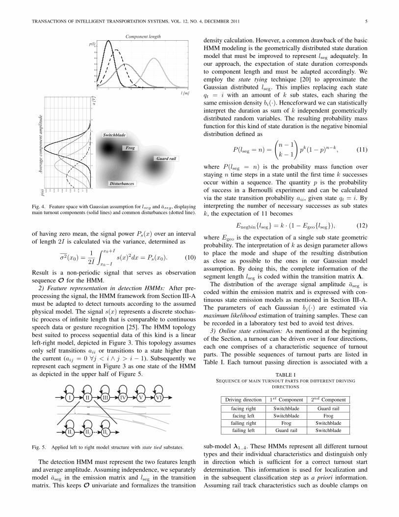
The ideal turnout model described in the beginning ofSection III involves several unknown parameters and additivenoise. The length lseg depends on different turnout types(for examples see [18]), speed estimation inaccuracies andadditional individual structural features for each turnout. Theaverage amplitude aseg is liable to filter effects, unpredictedbogie movements, clamp types, and varying sensor settings.Additional noise sources involve thermal noise and measure-ment effects. With this, we assume, due to the central limittheorem [19], an additive zero mean white Gaussian noise withindividual variance for the true parameters lseg and aseg. Asdepicted in Figure 4, the transformation in the two dimen-sional feature space discriminates each segment sufficientlyby its mean and variance. Mean and variance of the depictedGaussians are won from recorded test data via maximumlikelihood (ML) estimation [13] and the Gaussian assumptionsuccessfully confirmed by a χ2-test with significance levelof 5%. The biggest discriminative power lies in the maincomponent models II and V that are also depicted in Figure 3.They show a good separability to each other and can bedistinguished from open track areas and disturbances such ascables, metallic clutter or unique infrastructure such as bridges.The latter can have similar shape to turnout components,e.g. switchblades, but can be distinguished by knowledge ofthe turnout set-up. Turnouts are thus represented by both, adistinct sequence of components and their respective features.HMMs are perfectly suited to model the underlying turnoutsub-component sequence and their conditioned features. Inaddition, if the signal component space is discrete and finitethey are optimally in a Bayesian sense.

1) Signal preprocessing for turnout detection: In a pre-processing step the time domain signal is transformed tospatial space. This alleviates the velocity dependent signalstraining proportional to the quality of the speed estimation(see Section II-B). Afterwards, exploiting the signal property


Fig. 4. Feature space with Gaussian assumption for lseg and aseg , displayingmain turnout components (solid lines) and common disturbances (dotted line).

of having zero mean, the signal power Ps(x) over an intervalof length 2I is calculated via the variance, determined as

σ2(x0) =1

2I

∫ x0+I

x0−Is(x)2dx = Ps(x0). (10)

Result is a non-periodic signal that serves as observationsequence O for the HMM.

2) Feature representation in detection HMMs: After pre-processing the signal, the HMM framework from Section III-Amust be adapted to detect turnouts according to the assumedphysical model. The signal s(x) represents a discrete stochas-tic process of infinite length that is comparable to continuousspeech data or gesture recognition [25]. The HMM topologybest suited to process sequential data of this kind is a linearleft-right model, depicted in Figure 3. This topology assumesonly self transitions aii or transitions to a state higher thanthe current (aij = 0 ∀j < i ∧ j > i − 1). Subsequently werepresent each segment in Figure 3 as one state of the HMMas depicted in the upper half of Figure 5.

II VIVIIII IV

II2

II1

IIk

Fig. 5. Applied left to right model structure with state tied substates.

The detection HMM must represent the two features lengthand average amplitude. Assuming independence, we separatelymodel aseg in the emission matrix and lseg in the transitionmatrix. This keeps O univariate and formalizes the transition

density calculation. However, a common drawback of the basicHMM modeling is the geometrically distributed state durationmodel that must be improved to represent lseg adequately. Inour approach, the expectation of state duration correspondsto component length and must be adapted accordingly. Weemploy the state tying technique [20] to approximate theGaussian distributed lseg. This implies replacing each stateqt = i with an amount of k sub states, each sharing thesame emission density bi(·). Henceforward we can statisticallyinterpret the duration as sum of k independent geometricallydistributed random variables. The resulting probability massfunction for this kind of state duration is the negative binomialdistribution defined as

P (lseg = n) =

(n− 1

k − 1

)pk(1− p)n−k, (11)

where P (lseg = n) is the probability mass function overstaying n time steps in a state until the first time k successesoccur within a sequence. The quantity p is the probabilityof success in a Bernoulli experiment and can be calculatedvia the state transition probability aii, given state qt = i. Byinterpreting the number of necessary successes as sub statesk, the expectation of 11 becomes

Enegbin{lseg} = k · (1− Egeo{lseg}), (12)

where Egeo is the expectation of a single sub state geometricprobability. The interpretation of k as design parameter allowsto place the mode and shape of the resulting distributionas close as possible to the ones in our Gaussian modelassumption. By doing this, the complete information of thesegment length lseg is coded within the transition matrix A.

The distribution of the average signal amplitude aseg iscoded within the emission matrix and is expressed with con-tinuous state emission models as mentioned in Section III-A.The parameters of each Gaussian bj(·) are estimated viamaximum likelihood estimation of training samples. These canbe recorded in a laboratory test bed to avoid test drives.

3) Online state estimation: As mentioned at the beginningof the Section, a turnout can be driven over in four directions,each one comprises of a characteristic sequence of turnoutparts. The possible sequences of turnout parts are listed inTable I. Each turnout passing direction is associated with a

TABLE ISEQUENCE OF MAIN TURNOUT PARTS FOR DIFFERENT DRIVING

DIRECTIONS

Driving direction 1st Component 2nd Component

facing right Switchblade Guard railfacing left Switchblade Frog

failing right Frog Switchbladefailing left Guard rail Switchblade

sub-model λ1..4. These HMMs represent all different turnouttypes and their individual characteristics and distinguish onlyin direction which is sufficient for a correct turnout startdetermination. This information is used for localization andin the subsequent classification step as a priori information.Assuming rail track characteristics such as double clamps on


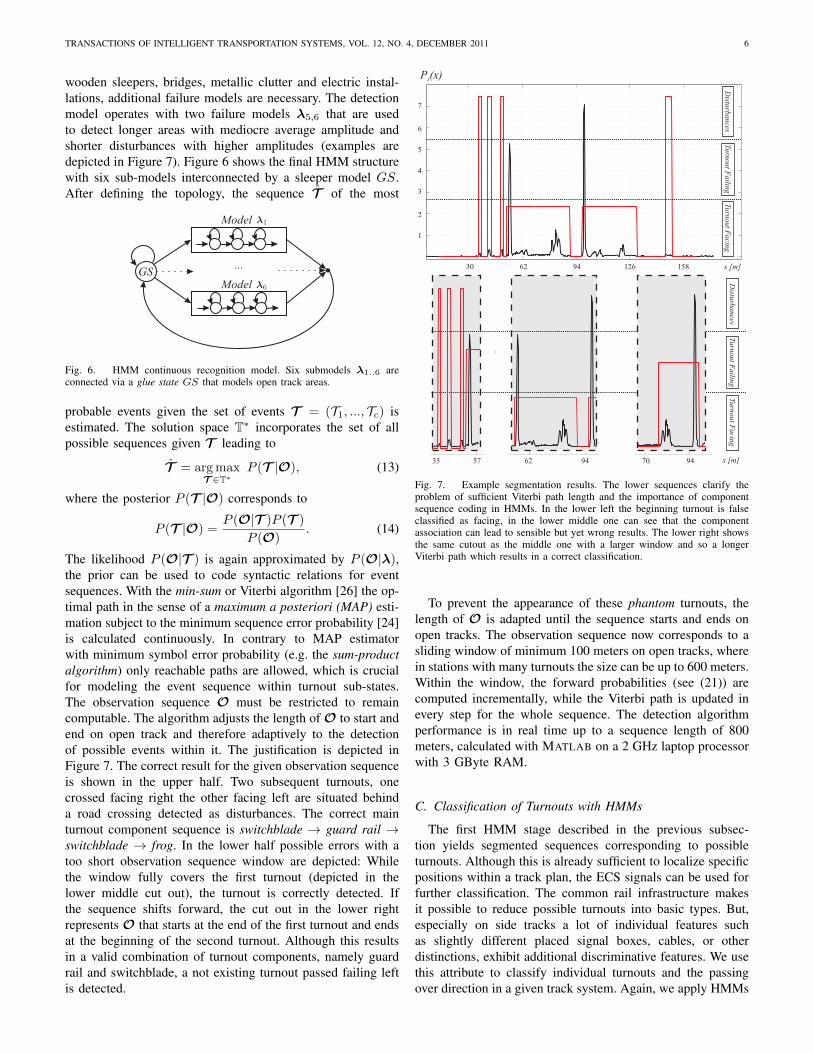
wooden sleepers, bridges, metallic clutter and electric instal-lations, additional failure models are necessary. The detectionmodel operates with two failure models λ5,6 that are usedto detect longer areas with mediocre average amplitude andshorter disturbances with higher amplitudes (examples aredepicted in Figure 7). Figure 6 shows the final HMM structurewith six sub-models interconnected by a sleeper model GS.After defining the topology, the sequence T of the most

Fig. 6. HMM continuous recognition model. Six submodels λ1..6 areconnected via a glue state GS that models open track areas.

probable events given the set of events T = (T1, ..., Tc) isestimated. The solution space T∗ incorporates the set of allpossible sequences given T leading to

T = arg maxT ∈T∗

P (T |O), (13)

where the posterior P (T |O) corresponds to

P (T |O) =P (O|T )P (T )

P (O). (14)

The likelihood P (O|T ) is again approximated by P (O|λ),the prior can be used to code syntactic relations for eventsequences. With the min-sum or Viterbi algorithm [26] the op-timal path in the sense of a maximum a posteriori (MAP) esti-mation subject to the minimum sequence error probability [24]is calculated continuously. In contrary to MAP estimatorwith minimum symbol error probability (e.g. the sum-productalgorithm) only reachable paths are allowed, which is crucialfor modeling the event sequence within turnout sub-states.The observation sequence O must be restricted to remaincomputable. The algorithm adjusts the length of O to start andend on open track and therefore adaptively to the detectionof possible events within it. The justification is depicted inFigure 7. The correct result for the given observation sequenceis shown in the upper half. Two subsequent turnouts, onecrossed facing right the other facing left are situated behinda road crossing detected as disturbances. The correct mainturnout component sequence is switchblade → guard rail →switchblade → frog. In the lower half possible errors with atoo short observation sequence window are depicted: Whilethe window fully covers the first turnout (depicted in thelower middle cut out), the turnout is correctly detected. Ifthe sequence shifts forward, the cut out in the lower rightrepresents O that starts at the end of the first turnout and endsat the beginning of the second turnout. Although this resultsin a valid combination of turnout components, namely guardrail and switchblade, a not existing turnout passed failing leftis detected.

Fig. 7. Example segmentation results. The lower sequences clarify theproblem of sufficient Viterbi path length and the importance of componentsequence coding in HMMs. In the lower left the beginning turnout is falseclassified as facing, in the lower middle one can see that the componentassociation can lead to sensible but yet wrong results. The lower right showsthe same cutout as the middle one with a larger window and so a longerViterbi path which results in a correct classification.

To prevent the appearance of these phantom turnouts, thelength of O is adapted until the sequence starts and ends onopen tracks. The observation sequence now corresponds to asliding window of minimum 100 meters on open tracks, wherein stations with many turnouts the size can be up to 600 meters.Within the window, the forward probabilities (see (21)) arecomputed incrementally, while the Viterbi path is updated inevery step for the whole sequence. The detection algorithmperformance is in real time up to a sequence length of 800meters, calculated with MATLAB on a 2 GHz laptop processorwith 3 GByte RAM.

C. Classification of Turnouts with HMMs

The first HMM stage described in the previous subsec-tion yields segmented sequences corresponding to possibleturnouts. Although this is already sufficient to localize specificpositions within a track plan, the ECS signals can be used forfurther classification. The common rail infrastructure makesit possible to reduce possible turnouts into basic types. But,especially on side tracks a lot of individual features suchas slightly different placed signal boxes, cables, or otherdistinctions, exhibit additional discriminative features. We usethis attribute to classify individual turnouts and the passingover direction in a given track system. Again, we apply HMMs


to cope with variations in the signals from bogie movements,sensor deterioration, and velocity estimation errors.

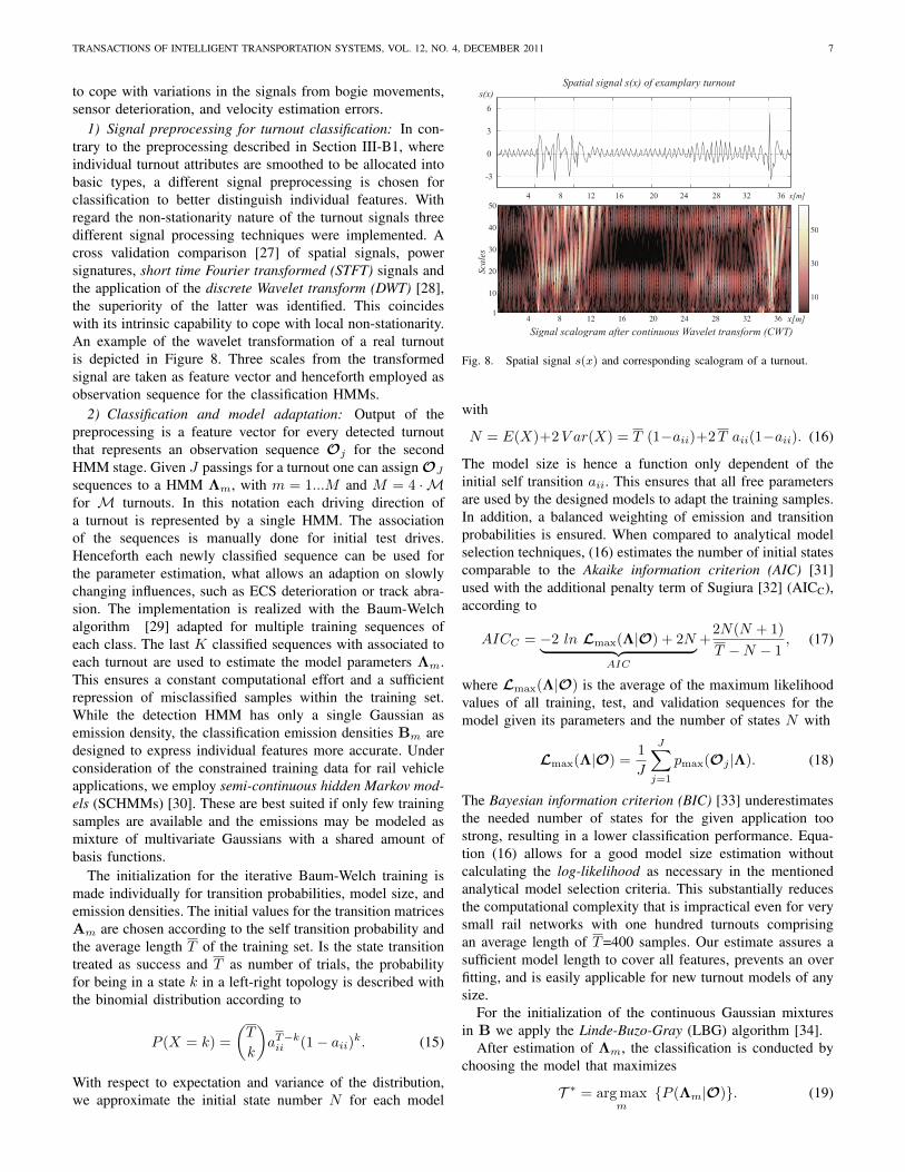
1) Signal preprocessing for turnout classification: In con-trary to the preprocessing described in Section III-B1, whereindividual turnout attributes are smoothed to be allocated intobasic types, a different signal preprocessing is chosen forclassification to better distinguish individual features. Withregard the non-stationarity nature of the turnout signals threedifferent signal processing techniques were implemented. Across validation comparison [27] of spatial signals, powersignatures, short time Fourier transformed (STFT) signals andthe application of the discrete Wavelet transform (DWT) [28],the superiority of the latter was identified. This coincideswith its intrinsic capability to cope with local non-stationarity.An example of the wavelet transformation of a real turnoutis depicted in Figure 8. Three scales from the transformedsignal are taken as feature vector and henceforth employed asobservation sequence for the classification HMMs.

2) Classification and model adaptation: Output of thepreprocessing is a feature vector for every detected turnoutthat represents an observation sequence Oj for the secondHMM stage. Given J passings for a turnout one can assign OJ

sequences to a HMM Λm, with m = 1...M and M = 4 · Mfor M turnouts. In this notation each driving direction ofa turnout is represented by a single HMM. The associationof the sequences is manually done for initial test drives.Henceforth each newly classified sequence can be used forthe parameter estimation, what allows an adaption on slowlychanging influences, such as ECS deterioration or track abra-sion. The implementation is realized with the Baum-Welchalgorithm [29] adapted for multiple training sequences ofeach class. The last K classified sequences with associated toeach turnout are used to estimate the model parameters Λm.This ensures a constant computational effort and a sufficientrepression of misclassified samples within the training set.While the detection HMM has only a single Gaussian asemission density, the classification emission densities Bm aredesigned to express individual features more accurate. Underconsideration of the constrained training data for rail vehicleapplications, we employ semi-continuous hidden Markov mod-els (SCHMMs) [30]. These are best suited if only few trainingsamples are available and the emissions may be modeled asmixture of multivariate Gaussians with a shared amount ofbasis functions.

The initialization for the iterative Baum-Welch training ismade individually for transition probabilities, model size, andemission densities. The initial values for the transition matricesAm are chosen according to the self transition probability andthe average length T of the training set. Is the state transitiontreated as success and T as number of trials, the probabilityfor being in a state k in a left-right topology is described withthe binomial distribution according to

P (X = k) =

(T

k

)aT−kii (1− aii)k. (15)

With respect to expectation and variance of the distribution,we approximate the initial state number N for each model

Fig. 8. Spatial signal s(x) and corresponding scalogram of a turnout.

with

N = E(X)+2V ar(X) = T (1−aii)+2T aii(1−aii). (16)

The model size is hence a function only dependent of theinitial self transition aii. This ensures that all free parametersare used by the designed models to adapt the training samples.In addition, a balanced weighting of emission and transitionprobabilities is ensured. When compared to analytical modelselection techniques, (16) estimates the number of initial statescomparable to the Akaike information criterion (AIC) [31]used with the additional penalty term of Sugiura [32] (AICC),according to

AICC = −2 ln Lmax(Λ|O) + 2N︸︷︷︸AIC

+2N(N + 1)

T −N − 1, (17)

where Lmax(Λ|O) is the average of the maximum likelihoodvalues of all training, test, and validation sequences for themodel given its parameters and the number of states N with

Lmax(Λ|O) =1

J

J∑j=1

pmax(Oj |Λ). (18)

The Bayesian information criterion (BIC) [33] underestimatesthe needed number of states for the given application toostrong, resulting in a lower classification performance. Equa-tion (16) allows for a good model size estimation withoutcalculating the log-likelihood as necessary in the mentionedanalytical model selection criteria. This substantially reducesthe computational complexity that is impractical even for verysmall rail networks with one hundred turnouts comprisingan average length of T=400 samples. Our estimate assures asufficient model length to cover all features, prevents an overfitting, and is easily applicable for new turnout models of anysize.

For the initialization of the continuous Gaussian mixturesin B we apply the Linde-Buzo-Gray (LBG) algorithm [34].

After estimation of Λm, the classification is conducted bychoosing the model that maximizes

T ∗ = arg maxm

{P (Λm|O)}. (19)


Here, T ∗ represents the associated turnout and its driving di-rection. Assuming an uniform prior over all possible turnouts,the posterior P (Λm|O) is proportional to the likelihood andcalculated with the forward algorithm [23] according to

p(O|Λm) =

N∑j=1

αT (j), (20)

αt(j) =

(N∑i=1

αt−1(i) · aij

)· bj(Ot), (21)

where αt(j) represents the probability of being in state qt = jat time step t, for likelihood computation.

IV. LOCALIZATION IN TOPOLOGICAL MAPS

Rail vehicles are not steerable and can be modeled withone degree of freedom preset by the rail network. With this,the train position is determined by the current track segment,the position upon it and the current driving direction. TheECS solves this with the combination of the velocity estimatevest(t) described in Section II and turnout extraction describedin Section III. Yet, the information must be merged withina map. We employ topological maps as natural choice torepresent a rail network. In our contribution a static mapwith known distances is assumed. The map can be set upwith basic information of edge length and turnout connectionsthat is accessible for every rail network. Although we implythat the on-board localization is solely based on the ECSsystem, our probabilistic framework can easily be enhancedwith additional sensors, e.g. satellite navigation systems orinertial measurement systems to fulfill further security aspects.

A. Map representation

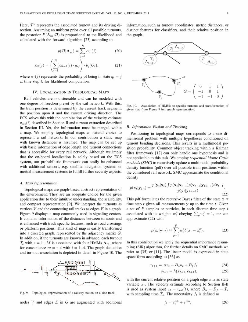
Topological maps are graph-based abstract representation ofthe environment. They are an adequate choice for the givenapplication due to their intuitive understanding, the scalability,and compact representation [9]. We interpret the turnouts asvertices V and the connecting rail tracks as edges E in a graph.Figure 9 displays a map commonly used in signaling centers.It contains information of the distances between turnouts andis enhanced with track specific features, such as road crossingsor platform positions. This kind of map is easily transformedinto a directed graph, represented by the adjacency matrix G.In addition, if the turnouts are known in advance, each turnoutTs with s = 1...M is associated with four HMMs Λm, wherefor convenience m = s, i with i = 1..4. The graph deductionand turnout association is depicted in detail in Figure 10. The

Fig. 9. Topological representation of a railway station on a side track.

nodes V and edges E in G are augmented with additional

information, such as turnout coordinates, metric distances, ordistinct features for classifiers, and their relative position inthe graph.

Fig. 10. Association of HMMs to specific turnouts and transformation ofgiven map from Figure 9 into graph representation.

B. Information Fusion and Tracking

Positioning in topological maps corresponds to a one di-mensional problem with multiple hypotheses conditioned onturnout bending decisions. This results in a multimodal po-sition probability. Common object tracking within a Kalmanfilter framework [12] can only handle one hypothesis and isnot applicable to this task. We employ sequential Monte Carlomethods (SMC) to recursively update a multimodal probabilitydensity function (pdf) over all possible train positions withinthe considered rail network. SMC approximate the conditionaldensity

p(xt|y1:t) =p(yt|xt)

∫p(xt|xt−1)p(xt−1|y1:t−1)dxt−1

p(yt|y1:t−1).

(22)This pdf formulates the recursive Bayes filter of the state x attime step t given all measurements y up to the time t. Givena set of P samples or particles, in each discrete time step tassociated with its weights wpt obeying

∑p w

pt = 1, one can

approximate (22) with

p(xt|y1:t) ≈P∑p=1

wpt δ(xt − xpt ). (23)

In this contribution we apply the sequential importance resam-pling (SIR) algorithm, for further details on SMC methods werefer to [35] or [11]. The linear model is expressed in statespace form according to [36] as

xt+1 = Axt +Buut +Bfft (24)yt+1 = h(xt+1, et+1), (25)

with the current relative position on a graph edge xrel as statevariable xt. The velocity estimate according to Section II-Bis used as system input ut = vest(t), where Bu = Bf = Tswith sampling time Ts. The uncertainty ft is defined as

ft = eestt + emo, (26)


and contains velocity uncertainty eestt ∼ N (0, (σestt )2), esti-

mated by the Kalman filter and additional constant Gaussianwhite noise emo ∼ N (0, (σmo)2) for model inaccuracies.

Each particle is additionally augmented with two pseudostates: The track segment IDt, corresponding to an edge Ewithin G, and its current driving direction dir defined asbinary variable. The pseudo states explicitly determine theposition in the map depending on xrel.

The measurement model (25) is nonlinear and reflectsdiscrete measurement events such as turnout detections. Weassume a constant zero mean Gaussian distribution for mea-surement uncertainty et+1 ∼ N (0, σ2), reflecting variations inthe detection HMM stage or misclassification. With this, (25)becomes

p(yt+1|xt+1) = N (d(xt+1)|µ = 0, σ2). (27)

The term d(xt+1) in (27) expresses the distance to the near-est node, given the current state and edge length l(IDt+1)according to

d(xt+1) =

{l(IDt+1) · xt+1, xt+1 < 0.5

|l(IDt+1) · (xt+1 − 1)|, xt+1 > 0.5. (28)

The state space formulation combined with SMC approx-imation allows an elegant incorporation of turnout drivingrestrictions stored in the map G. Detection and classificationprobabilities are directly integrated in the particle weightsin (23). The complete formulation is kept compact and canbe augmented easily.

For localization it is sufficient to subsequently detectturnouts and estimate the driven distance between to excludestep by step false hypotheses. For this case only velocityestimation and the detection HMM (see Section III-B) arenecessary to accomplish the localization. If turnouts are addi-tionally associated to individual HMMs as described in III-C,an instantaneous localization is possible. The employment ofthe classification HMMs comes at the cost of needed priorknowledge of track topology and the necessity of turnoutsthat exhibit discriminative features. Depending on this, twoscenarios can be distinguished:

• Side track scenario: Side tracks are characterized by fewstations and turnouts and relatively long spaces of over1 km between them. The turnouts differ in type andoccurrence and comprise individual features like signalbox wires, axle counters, and others. Therefore even twoturnouts of the same type are distinguishable as seen inSection III-C.

• Classification yard scenario: Rail yards and other freightspecific surroundings are specified by a significant higherturnout density. They are often laid nearly identically,being of same type. The distances between turnoutsare typically small but different. An example setup isshown in Figure 11, that displays only a small area ofa classification yard near Ludwigshafen.

Both scenarios are intrinsically solvable with our approach bychoosing the HMM input accordingly.

Fig. 11. Cutout of a classification yard near Ludwigshafen showing the vastamount of laid turnouts (black triangles) and its challenges for the shunt yardscenario.

V. EXPERIMENTAL RESULTS

All proposed algorithms were verified with real data. Thesewere recorded on a test train that operates on a secondarytrack. It incorporates roughly 22km track length, seven stationsand an overall of 54 turnouts. In test runs we were passingrepeatedly six stations and 23 turnouts in different directions.

A. Velocity Estimation

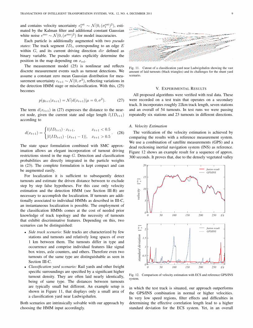
The verification of the velocity estimation is achieved bycomparing the results with a reference measurement system.We use a combination of satellite measurements (GPS) and adead reckoning inertial navigation system (INS) as reference.Figure 12 shows an example result for a sequence of approx.300 seconds. It proves that, due to the densely vegetated valley

Fig. 12. Comparison of velocity estimation with ECS and reference GPS/INSsystem.

in which the test track is situated, our approach outperformsthe GPS/INS combination in normal or higher velocities.In very low speed regions, filter effects and difficulties indetermining the effective correlation length lead to a higherstandard deviation for the ECS system. Yet, in an overall


comparison, the ECS approach in Section II-B proves morereliable and robust in average.

B. HMM Results

The algorithms and models described in Sections III-B andIII-C are evaluated separately, indicating that a localization ispossible with only applying the detection HMM.

1) HMMs for Detection: To verify the detection capabil-ities of our approach, we run 26 test drives (52 passingsof the turnouts) on the side track. The employed HMM isconstructed according to Figure 6 and consists of 196 statesand six submodels as described in Section III-B. The emissiondensities where estimated out of a set of real turnout signalswith manually labeled components. An overall of 845 trueturnout events are present on the test track, of which 831 weredetected correctly given only one false positive, which yieldsan overall recognition rate of 98.23% for solely detection.Moreover, we evaluated the driving direction preclassificationin the detection step. From the 831 properly detected turnouts774 were positively classified in the correct driving directionwhen distinguished in facing and failing. This corresponds toa classification rate of 93.14%.

2) HMMs for Classification: The same data set was ex-amined for classification performance. The data set was con-strained on turnouts, respectively classes, with at least 20passings to ensure a correct data set separation in training, vali-dation, and test set. This preselection left an overall of M = 34classes. The output of the second HMM stage yields a specificturnout and therefore node V , as well as a specific drivingdirection described in Table I, in contrast to the preclassifyingof the detection HMM that separates only in facing/failing andan unspecified turnout. The SCHMM emission densities wereset with 13 mixture components for a three dimensional inputvector consisting of bior wavelet family scales. The averagemodel size N is 232 states, given an average length T = 423.2of O. The maximum iterations of the Baum-Welch algorithmwere set to 15, whereas the number of training observationsequences K were set to nine. The overall error is computedon the test and validation sets that contain 277 turnout events.One false positive results in a classification performance of99.64%. Additional examinations showed that the approach isrobust up to a velocity estimation error of 15%.

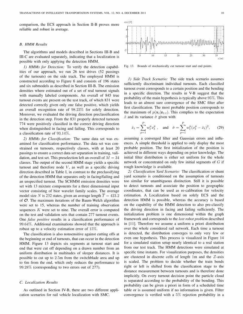
The classification is also nonsensitive against cutting offs atthe beginning or end of turnouts, that can occur in the detectionHMM. Figure 13 depicts six segments at turnout start andend that were cut off depending on a drawn number from anuniform distribution in multitudes of sleeper distances. It ispossible to cut up to 2.5m from the switchblade area and upto 6m from the end, which only reduces the performance to99.28% (corresponding to two errors out of 277).

C. Localization Results

As outlined in Section IV-B, there are two different appli-cation scenarios for rail vehicle localization with SMC.

Fig. 13. Bounds of stochastically cut turnout start and end points.

1) Side Track Scenario: The side track scenario assumessufficiently discriminant individual turnouts. Each classifiedturnout event corresponds to a certain position and the bendingin a specific direction. The results in V-B suggest that theprobability of the main hypothesis is typically above 95%. Thisleads to an almost sure convergence of the SMC filter afterfirst classification. The most probable position corresponds tothe maximum of p(xt|z1:t). This complies to the expectationx and its variance σ given with

xt =

P∑p=1

wpt xpt , and σ =

P∑p=1

wpt (xpt − xt)2, (29)

assuming a converged filter and Gaussian errors and influ-ences. A simple threshold is applied to only display the mostprobable position. The first initialization of the position isachieved in different ways depending on prior knowledge. Theinitial filter distribution is either set uniform for the wholenetwork or concentrated on only few initial segments of G ifrough knowledge is available.

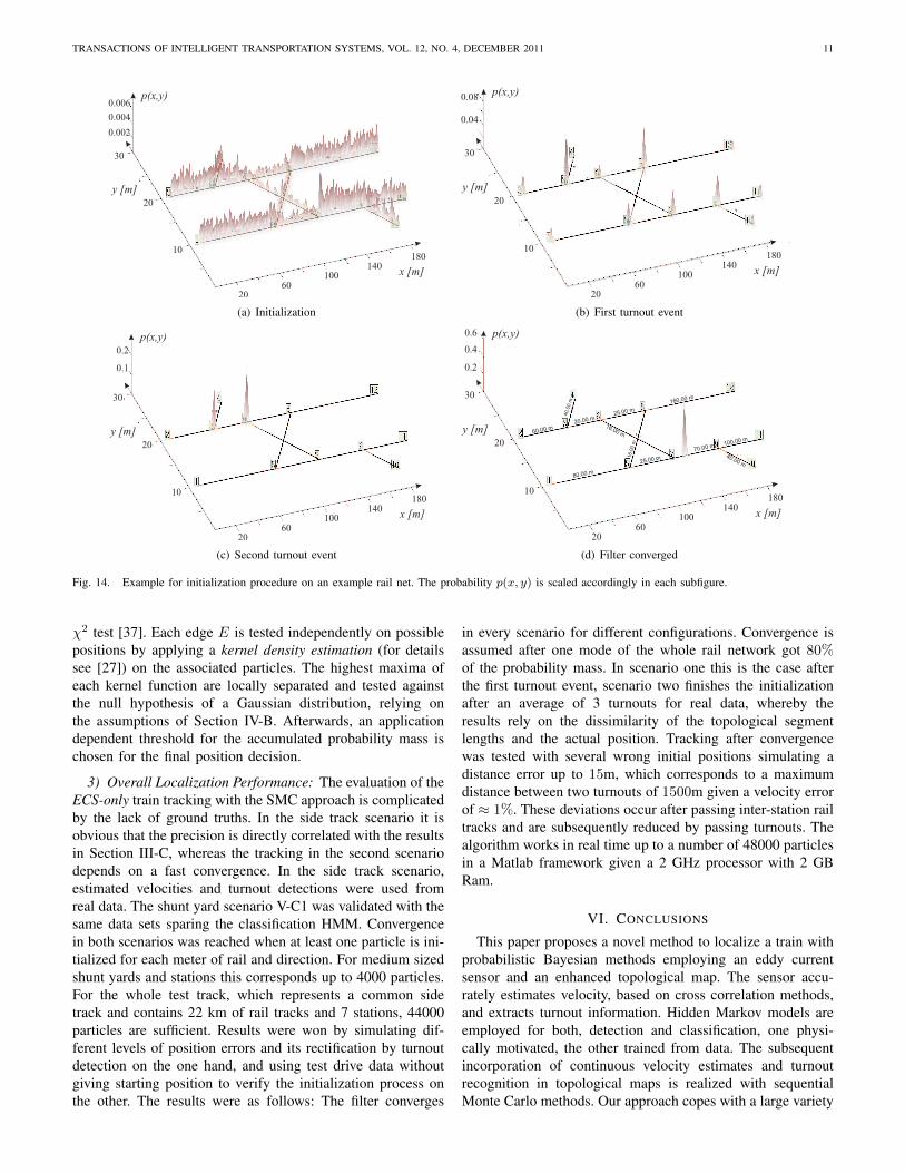
2) Classification Yard Scenario: The classification or shuntyard scenario is conditioned on the assumption of turnoutstoo similar for unambiguous distinction. Still it is possibleto detect turnouts and associate the position to geographiccoordinates, that can be used as re-calibration for velocityestimation. A Localization based on solely ECS and thedetection HMM is possible, whereas the accuracy is basedon the capability of the HMM detection to also pre-classifythe driving direction in facing and failing sufficiently. Theinitialization problem is one dimensional within the graphframework and corresponds to the lost robot problem describedin [11]. Therefore we assume a uniform a priori distributionover the whole considered rail network. Each time a turnoutis detected, the distribution converges to only very few oreven one hypothesis. This process is visualized in Figure 14for a simulated station setup nearly identical to a real stationfrom our test track. The HMM detections were simulated atspecific time instants. For visualization purposes, the densitiesare clustered in discrete cells of length 1m and the Z-axisis scaled. The problem to decide whether the train bendsright or left is shifted from the classification stage to thedistance measurement between turnouts and is therefore doneimplicitly. On every turnout decision point the particle cloudis separated according to the probability of the bending. Thisprobability can be given a priori in form of a scheduled timetable or is assumed uniform if no information is given. Filterconvergence is verified with a 5% rejection probability in a


(a) Initialization (b) First turnout event

(c) Second turnout event (d) Filter converged

Fig. 14. Example for initialization procedure on an example rail net. The probability p(x, y) is scaled accordingly in each subfigure.

χ2 test [37]. Each edge E is tested independently on possiblepositions by applying a kernel density estimation (for detailssee [27]) on the associated particles. The highest maxima ofeach kernel function are locally separated and tested againstthe null hypothesis of a Gaussian distribution, relying onthe assumptions of Section IV-B. Afterwards, an applicationdependent threshold for the accumulated probability mass ischosen for the final position decision.

3) Overall Localization Performance: The evaluation of theECS-only train tracking with the SMC approach is complicatedby the lack of ground truths. In the side track scenario it isobvious that the precision is directly correlated with the resultsin Section III-C, whereas the tracking in the second scenariodepends on a fast convergence. In the side track scenario,estimated velocities and turnout detections were used fromreal data. The shunt yard scenario V-C1 was validated with thesame data sets sparing the classification HMM. Convergencein both scenarios was reached when at least one particle is ini-tialized for each meter of rail and direction. For medium sizedshunt yards and stations this corresponds up to 4000 particles.For the whole test track, which represents a common sidetrack and contains 22 km of rail tracks and 7 stations, 44000particles are sufficient. Results were won by simulating dif-ferent levels of position errors and its rectification by turnoutdetection on the one hand, and using test drive data withoutgiving starting position to verify the initialization process onthe other. The results were as follows: The filter converges

in every scenario for different configurations. Convergence isassumed after one mode of the whole rail network got 80%of the probability mass. In scenario one this is the case afterthe first turnout event, scenario two finishes the initializationafter an average of 3 turnouts for real data, whereby theresults rely on the dissimilarity of the topological segmentlengths and the actual position. Tracking after convergencewas tested with several wrong initial positions simulating adistance error up to 15m, which corresponds to a maximumdistance between two turnouts of 1500m given a velocity errorof ≈ 1%. These deviations occur after passing inter-station railtracks and are subsequently reduced by passing turnouts. Thealgorithm works in real time up to a number of 48000 particlesin a Matlab framework given a 2 GHz processor with 2 GBRam.

VI. CONCLUSIONS

This paper proposes a novel method to localize a train withprobabilistic Bayesian methods employing an eddy currentsensor and an enhanced topological map. The sensor accu-rately estimates velocity, based on cross correlation methods,and extracts turnout information. Hidden Markov models areemployed for both, detection and classification, one physi-cally motivated, the other trained from data. The subsequentincorporation of continuous velocity estimates and turnoutrecognition in topological maps is realized with sequentialMonte Carlo methods. Our approach copes with a large variety


of turnouts in shape and style, mechanic and electromag-netic disturbances, misclassification and longitudinal drift. TheBayesian tracking is capable to compensate misclassificationsand velocity errors to robustly estimate the position and canbe used to reconstruct the driven path even in large railroadnetworks. Our framework can easily be augmented by addi-tional track characteristics or additional sensors if necessary.Future work will incorporate additional ECS information suchas the discrete number of sleepers in each segment to combinespatial and time information in one position estimate.

ACKNOWLEDGMENT

The authors would like to thank the German Federal Min-istry of Economics and Technology (BMWi), BombardierSweden, and the Karlsruher Verkehrsbetriebe.

REFERENCES

[1] P. Winter, J. Braband, and P. de Cicco, Compendium on ERTMS:European Rail Traffic Management System. UIC International, 2009.

[2] F. Bohringer, “Train location based on fusion of satellite and train-borne sensor data,” in Location Services and Navigation Technologies,vol. 5084, pp. 76–85, 2003.

[3] P. McIntire and R. C. McMaster, Nondestructive Testing Handbook, Vol.4. The American Society for Nondestructive Testing, Columbus, Ohio,1986.

[4] T. Engelberg and F. Mesch, “Eddy current sensor system for non-contactspeed and distance measurement of rail vehicles,” in Computers inRailways VII, pp. 1261–1270, WIT Press, 2000.

[5] F. Bohringer and A. Geistler, “Comparison between different fusionapproaches for train-borne location systems,” in Proc. IEEE Conferenceon Multisensor Fusion and Integration for Intelligent Systems, pp. 267–272, 2006.

[6] F. Kaleli and Y. Akgul, “Vision-based railroad track extraction usingdynamic programming,” in Proc. IEEE Conference on Intelligent Trans-portation Systems, 2009.

[7] S. S. Saab, “A map matching approach for train positioning. parti: Development and analyisis,” in IEEE Transaction On VehicularTechnology, vol. 49, pp. 467–475, 2000.

[8] S. S. Saab, “A map matching approach for train positioning. part ii:Application and expermentation,” in IEEE Transaction On VehicularTechnology, vol. 49, pp. 476–484, 2000.

[9] A. Ranganathan, Probabilistic Topological Maps. PhD thesis, GeorgiaInstitute of Technology, March 2008.

[10] B. Kuipers, “The spatial semantic hierarchy,” Artifical Intelligence,vol. 119, no. 1-2, pp. 191 – 233, 2000.

[11] S. Thrun, W. Burgard, and D. Fox, Probabilistic Robotics. Cambridge:The MIT Press, 2005.

[12] Y. Bar-Shalom, Multitarget/Multisensor Tracking: Applications and Ad-vances, vol. 3. Norwood: Artech House, 2000.

[13] C. Bishop, Pattern Recognition and Machine Learning. InformationScience and Statistics, 2006.

[14] F. Puente Lon and T. Engelberg, “Model-based sensing of track com-ponents for location of rail vehicles,” in Proc. of the IMTC, 2005.

[15] A. Geistler and F. Bohringer, “Robust velocity measurement for railwayapplications by fusing eddy current sensor signals,” in Proc. IEEEIntelligent Vehicles Symposium, (New York), pp. 664–669, IEEE, 2004.

[16] T. Strauss, C. Hasberg, and S. Hensel, “Correlation based velocityestimation during accelaration phases with application in rail vehicles,”in IEEE/SP 15th Workshop on Statistical Signal Processing, 2009.

[17] G. Welch and G. Bishop, “An introduction to the kalman filter,” inSIGGRAPH 2001, p. Course 8, University of North Carolina, 2001.

[18] W. W. Hay and C. Hay, Railroad Engineering. John Wiley & Sons,1982.

[19] A. Papoulis, Probability, Random Variables, and Stochastic Processes.Mcgraw-Hill Higher Education, 4 th ed., 2002.

[20] J. Bilmes, “What HMMs can do,” tech. rep., University of Washington,2002.

[21] R. Durbin, Biological sequence analysis. Cambridge University Press,2002.

[22] S. P. Chatzis, D. I. Kosmopoulos, and T. A. Varvarigou, “Robust sequen-tial data modeling using an outlier tolerant hidden markov model,” IEEETransactions on Pattern Analysis and Machine Intelligence, vol. 31,pp. 1657–1669, September 2009.

[23] L. Rabiner, “A tutorial on hidden Markov models and selected applica-tions in speech recognition,” Proceedings of the IEEE, vol. 77, pp. 257–286, 1989.

[24] Y. Ephraim and N. Merhav, “Hidden markov processes,” IEEE Trans-actions on Information Theory, vol. 48, pp. 1518 – 1569, June 2002.

[25] M. Ghil, M. R. Allen, A. D. Dettinger, K. Ide, and D. Kondrashov,“Advanced spectral methods for climatic time series,” Reviews of Geo-physics, vol. 40, pp. 1 – 41, 2002.

[26] A. Viterbi, “Error bounds for convolutional codes and an asymptoti-cally optimum decoding algorithm,” IEEE Transactions on InformationTheory, vol. 5, pp. 260–269, 1967.

[27] T. Hastie, R. Tibshirani, and J. Friedman, The Elements of StatisticalLearning. Springer, 2001.

[28] S. Mallat, A Wavelet Tour of Signal Processing. Academic Press, 2 ed.,1999.

[29] L. E. Baum, “An inequality and associated maximization technique instatistical estimation for probabilistic functions of markov processes,”Inequalities III, pp. 1 – 8, 1972.

[30] X. D. Huang and M. Jack, “Semi-continuous hidden markov modelsfor speech recognition,” Computer Speech and Language, vol. 3, no. 3,pp. 239 – 251, 1989.

[31] H. Akaike, “Information measures and model selection,” Bulletin of theinternational statistical Institute, vol. 50, pp. 277 – 290, 1983.

[32] N. Sugiura, “Further analysis of the data by akaike’s informationcriterion and the finite corrections,” Communications in Statistics -Theory and Methods, vol. A7, pp. 13 – 26, 1978.

[33] E. T. Jaynes, Probability Theory the logic of science. CambridgeUniversity Press, 2003.

[34] Y. Linde, A. Buzo, and R. M. Gray, “An algorithm for vector quantizerdesign,” IEEE Transactions on communications, vol. 28, pp. 84–95,January 1980.

[35] S. Arulampalam, “A Tutorial on Particle Filters for OnlineNonlinear/Non-Gaussian Bayesian Tracking,” IEEE Transactions onSignal Processing, vol. 50, pp. 174 – 188, 2002.

[36] F. Gustafsson and al., “Particle filters for positioning, navigation andtracking,” IEEE Transactions on Signal Processing, vol. 50, pp. 425 –436, 2002.

[37] L. Grafakos, Classical and Modern Fourier Analysis. Pearson Education,2004.

Stefan Hensel (S’09) received the Diploma in me-chanical engineering at the University of Karlsruhe,Germany, in 2006. His research interest lie in statis-tical signal processing and pattern recognition withapplications in eddy current sensor technology fortrain application systems. He is currently working atthe Institute of Measurement and Control Systems,Karlsruhe Institute of Technology (KIT).

Carsten Hasberg (S’10) studied electrical engi-neering at the University of Karlsruhe, Germany.He received the Dipl.-Ing. degree at University ofKarlsruhe, Germany in 2006. His research inter-est lies in localization technology for autonomoussystems. He is currently working at the Instituteof Measurement and Control Systems, KarlsruheInstitute of Technology (KIT).


Christoph Stiller (S’93M’95SM’99) studied elec-trical engineering at the Universities in Aachen,Germany, and Trondheim, Norway. He received theDr.-Ing. degree (Ph.D.) with distinction from AachenUniversity in 1994. He worked in the ResearchDepartment, INRS-Telecommunications, Montreal,QC, Canada, and in advanced development forRobert Bosch GmbH, Hildesheim, Germany. In2001, he became a chaired Professor and Head ofthe Institute for Measurement and Control Systemsat the Karlsruhe Institute of Technology (KIT), Ger-

many. His present interests cover cognition of mobile systems, computervision, and real-time applications thereof. He is the author or coauthor of morethan 100 publications and patents in these fields. Dr. Stiller is Vice PresidentMember Activities of the IEEE Intelligent Transportation Systems Society.He served as Associate Editor for the IEEE TRANSACTIONS ON IMAGEPROCESSING (1999 2003) and, since 2004, for the IEEE TRANSACTIONSON INTELLIGENT TRANSPORTATION SYSTEMS. In January 2009, hewas nominated Editor-in-Chief of the IEEE Intelligent Transportation SystemsMagazine. He is the Speaker of the Transregional Collaborative ResearchCenter Cognitive Automobiles of the German Research Foundation..

Documents

TRANSACTIONS OF INTELLIGENT … OF INTELLIGENT TRANSPORTATION SYSTEMS, VOL. 12, NO. 4, DECEMBER 2011 1 Probabilistic Rail Vehicle Localization with Eddy Current Sensors in Topological