Alonzo Kelly Reactive Nonholonomic Bryan Nagy …alonzo/pubs/papers/ijrr02TrajGen.pdfTrajectory Generation via Parametric ... Kelly and Nagy / Reactive Nonholonomic Trajectory Generation

Alonzo KellyBryan NagyRobotics InstituteCarnegie Mellon UniversityPittsburgh, PA 15213-3890, [email protected]@rec.ri.cmu.edu

Reactive NonholonomicTrajectory Generationvia ParametricOptimal Control

Abstract

There are many situations for which a feasible nonholonomic motionplan must be generated immediately based on real-time perceptualinformation. Parametric trajectory representations limit computa-tion because they reduce the search space for solutions (at the costof potentially introducing suboptimality). The use of any parametrictrajectory model converts the optimal control formulation into anequivalent nonlinear programming problem. In this paper, curva-ture polynomials of arbitrary order are used as the assumed formof solution. Polynomials sacrifice little in terms of spanning the setof feasible controls while permitting an expression of the generalsolution to the system dynamics in terms of decoupled quadratures.These quadratures are then readily linearized to express the neces-sary conditions for optimality. Resulting trajectories are convenientto manipulate and execute in vehicle controllers and they can becomputed with a straightforward numerical procedure in real time.

KEY WORDS—mobile robots, car-like robots, trajectorygeneration, curve generation, nonholonomic, clothoid, cornuspiral, optimal control

1. Introduction

Trajectory generation is a more difficult problem than it may atfirst appear to be. By contrast to manipulation, where the com-mon inverse problem is that of inverting nonlinear kinematicequations, the common inverse problem for mobile robots isthat of inverting nonlinear differential equations.

1.1. Notation

For a vehicle actuated in curvature and speed while movingin the plane, one description of its dynamics is the followingfour coupled, nonlinear equations:

The International Journal of Robotics ResearchVol. 22, No. 7–8, July–August 2003, pp. 583-601,©2003 Sage Publications

x(t) = V (t) cosθ(t) θ (t) = κ(t)V (t)

y(t) = V (t) sinθ(t) κ(t) = u(t). (1)

The vehicle state vector (also called a posture in this context)consists of the position coordinates(x, y), headingθ , andcurvatureκ:

x = (x, y, θ, κ)T. (2)

The input or control vector consists of speedV and desiredcurvatureu:

u = (V , u)T. (3)

It is straightforward to effect a change of variable from timeto distance. Integrating the equations produces a canonicalexpression of the equations of odometric dead reckoning:

x(s) =s∫

0

cosθ(s)ds θ(s) =s∫

0

κ(s)ds

y(s) =s∫

0

sinθ(s)ds κ(s) = u(s). (4)

These equations are not a solution in the classical differentialequation sense because the heading (a state) appears insidethe integrals.

1.2. Problem Statement

The forward problem is that of determining the state spacetrajectory from the input functions. This problem is equivalentto dead reckoning and it can be solved by integrating theabove equations numerically. It is not possible to computethe position without simultaneously computing the heading,because the above is not formally a solution.

In this paper we address the inverse problem. In the in-verse problem, all or part of the state space trajectoryx is

583

http:\\www.sagepublications.com

584 THE INTERNATIONAL JOURNAL OF ROBOTICS RESEARCH / July–August 2003

specified, and the associated controlu (input function) mustbe computed. The question of whether such au exists whenboundary conditions are specified is one of classical control-lability. When more than one such input exists, it becomespossible to think about optimizing some performance index(such as smoothness) and the problem becomes one of optimalcontrol.

Unlike in the case of holonomic motion planning, obsta-cles are not required in order to make the problem of non-holonomic trajectory generation difficult. The terms trajec-tory generation, trajectory planning, and nonholonomic mo-tion planning have been used historically for the problem ofachieving goal postures while respecting dynamic and non-holonomic limitations on mobility. In many cases, quantitiesto be optimized are introduced and, less frequently, knownobstacles are introduced to generate additional constraints onmobility and require higher degrees of search.

Much of the work to date has either expressed the problemstrictly in terms of goal posture acquisition or assumed that theenvironment was known a priori. Yet, every time that an op-erating vehicle must react to its environment based on sensedinformation gathered while on the move, a nonholonomic mo-tion plan must be generated in real time. Indeed, our work inapplications points to a strong need for feasible motion plansto be generated virtually instantaneously in response to newlyacquired environmental information. In this paper, we addressthe need to generate such reactive trajectories in real time.

1.3. Motivation

Real-time trajectory generation is motivated by applicationsof precision control. While computing trajectories is a com-plicated matter, there are many situations for which nothingless will solve the problem. Due to dynamics, limited cur-vature, and underactuation, a vehicle often has few optionsfor how it travels over the space immediately in front of it.The key to achieving a relatively arbitrary posture is to thinkabout doing so well before getting there, and to do so basedon precise understanding of the above limitations.

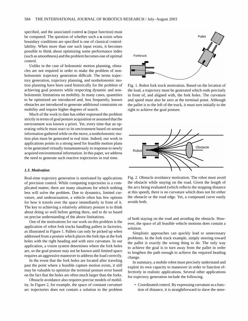
One of the motivations for our work on this problem is theapplication of robot fork trucks handling pallets in factories,as illustrated in Figure 1. Pallets can only be picked up whenaddressed from a posture which places the fork tips at the forkholes with the right heading and with zero curvature. In ourapplication, a vision system determines where the fork holesare, so the goal posture may not be known until limited spacerequires an aggressive maneuver to address the load correctly.

In the event that the fork holes are located after travelingpast the point where a feasible capture motion exists, it stillmay be valuable to optimize the terminal posture error basedon the fact that the holes are often much larger than the forks.

Obstacle avoidance also requires precise models of mobil-ity. In Figure 2, for example, the space of constant curvaturearc trajectories does not contain a solution to the problem

Pallet

Forktruck

Fig. 1. Robot fork truck motivation. Based on the location ofthe load, a trajectory must be generated which ends preciselyin front of, and aligned with, the fork holes. The curvatureand speed must also be zero at the terminal point. Althoughthe pallet is to the left of the truck, it must turn initially to theright to achieve the goal posture.

ObstacleRobot

Fig. 2. Obstacle avoidance motivation. The robot must avoidthe obstacle while staying on the road. Given the length ofthe arcs being evaluated (which reflects the stopping distanceat this speed), there is no curvature which does not hit eitherthe obstacle or the road edge. Yet, a compound curve easilyavoids both.

of both staying on the road and avoiding the obstacle. How-ever, the space of all feasible vehicle motions does contain asolution.

Simplistic approaches can quickly lead to unnecessaryproblems. In the fork truck example, simply steering towardthe pallet is exactly the wrong thing to do. The only wayto achieve the goal is to turn away from the pallet in orderto lengthen the path enough to achieve the required headingchange.

In summary, a mobile robot must precisely understand andexploit its own capacity to maneuver in order to function ef-fectively in realistic applications. Several other applicationsfor trajectory generation include the following.

• Coordinated control. By expressing curvature as a func-tion of distance, it is straightforward to slave the steer-

Kelly and Nagy / Reactive Nonholonomic Trajectory Generation 585

ing wheel to the actual distance traveled in order toensure that the intended trajectory is being followed.

• Planned obstacle avoidance. Due to the availabilityof the Jacobian matrix with respect to the trajectoryparameters, it becomes straightforward to computefirst-order modifications to a planned trajectory whichmoves it outside the region of intersection with anobstacle.

• Guidepath representation. Many factory automation ve-hicles express vehicle guidepaths (the robot roads inthe factory) in terms of lines and arcs; the more gen-eral primitives computed here are a more effectiverepresentation.

• Path following. Corrective trajectories for path follow-ing applications can be generated in such a manner asto achieve the correct position, heading, and curvatureof the point of path re acquisition.

For trajectories which achieve curvature and higher or-ders of continuity when joined together, prohibitive rapid ac-cess storage would be required to implement lookup tablesof solutions for a high-density sampling of every terminalpose within a useful range. While interpolation can be usedto reduce storage requirements, the algorithm presented herecan compute solutions so rapidly from such poor initial esti-mates that it would often render even tables of initial guessesunnecessary.

While advances in computing continue to render slower al-gorithms faster, the value of efficient nonholonomic trajectorygeneration is not restricted to computers of the contemporarygeneration. In the context of planning around obstacles, whereup to thousands of trajectories per second are checked for col-lisions, an efficient generator enables an efficient planner.

1.4. Prior Work

From a robotics perspective, there has been little work onthis problem when compared with, for example, the amountof effort devoted to localization (position estimation). Fromanother, the two-point boundary value problem of differentialequations, optimal curves in the calculus of variations, thespline generation problem of geometric modeling, and theoptimal control problem are all very closely related and oftenmore general problems.

Some of the earliest work in robotics appeals to the appliedmathematics literature to supply a precedent for the problem(Horn 1983; Dubins 1957).

Contemporary applied mathematics literature addressesthe relationships between abstract curve generation and con-trol. For example, the relationship between curve fitting andoptimal control is addressed in Kano et al. (2003). Here, theuse of linear system dynamics to fit curves is first attributedto practitioners in flight control.

Early approaches in robotics are characterized by a curve-fitting formulation where the parameter space of a family ofone or more curves of some assumed general form is searchedfor a solution. With the exception of very early work whichused B-splines, researchers initially preferred to represent tra-jectories in terms of heading, curvature, and higher deriva-tives, presumably due to their ease of execution and the easewith which curvature constraints can be tested, if not imposed.

The progression is from line segments (Tsumura et al.1981) to arcs (Komoriya, Tachi, and Tanie 1984) to clothoids(Kanayama and Miyake 1985) to cubic spirals (quadratic cur-vature) (Kanayama and Hartman 1988). The progression toever higher-order polynomials reflects the desire to constrainhigher-order derivatives for boundary values, and therebyachieve higher levels of continuity when primitives are joinedtogether sequentially.

Aspects of optimization have appeared over time. InKanayama and Miyake (1985) is an early mention of thenonuniqueness of solutions and searching alternatives. InKanayama and Hartman (1988) are explicit performance in-dices and proofs of optimality for clothoids and cubic spirals.

One approach to planning is to sequence atomic primitivestogether. Dubins (1957) showed that sequences of arcs andlines are shortest for a forward moving vehicle given a con-straint on average curvature. Much later, Reeds and Shepp(1990) generalized this result to forward and backward mo-tions, and Shkel and Lumelsky (1996) used classification toimprove efficiency.

These works have been restricted to line and arc primitivesbased on the quest for the shortest path, but in the presence ofobstacles or higher-order boundary conditions, more expres-sive primitives are required. Earlier Shin and Singh (1990) forexample, composed trajectories from clothoids and lines forthese reasons.

Boisonnat, Cérézo, and Leblond (1992) derived Dubin’sresult using variational principles. Variational methods arenow commonly applied to nonholonomic motion planning inrobotics (Latombe 1991; Laumond 1998). The relationship tothe two-point boundary value problem has meant that clas-sical numerical methods are applicable. Delingette, Herbert,and Ikeuchi (1991) use a sampled representation of the tra-jectory and a relaxation based numerical method to computethe optimum input.

The shooting method is another classical technique forsolving boundary value and optimal control problems. It isbased on assuming a parametric representation and solving forthe parameters. The method of substituting a family of curvesinto a differential equation and solving for the parameters is,of course, classical “variation of parameters”. Likewise, theuse of power series in order to solve differential equations hasbeen employed for centuries.

From as early as Brockett (1981) it has been known that si-nusoidal inputs are optimal from the perspective of minimizedsquared effort. Murray and Sastry (1993) used this result to


generate suboptimal solutions for chained systems. Similarly,Fernandes, Gurvits, and Li (1991) proposed the use of a trun-cated Fourier series to express the steering input and proposea shooting method to find the coefficients of these sinusoidalbasis functions. Polynomial steering functions have been pro-posed in Tilbury, Murray, and Sastry (1995) for steering in then trailer problem.

Much of the nonholonomic motion planning literature hasbecome theoretical in nature and algorithmic efficiency is notoften discussed. In Reuter (1998), however, a near real-timeoptimal control solution appears. The problem is formulatedas eleven simultaneous first-order differential equations sub-ject to boundary conditions which include curvature and itsderivative. Solutions are generated in about 1/3 s.

1.5. Approach

The approach presented in this paper is one which combinesmany of the strengths of earlier techniques in order to achieveboth a highly general formulation and a real-time solution.First, the clothoid and related curves of earlier approaches aregeneralized to a curvature polynomial of arbitrary order whichbecomes the assumed form of the solution. This form of so-lution presents several computational advantages. Secondly,the very general optimal control formulation is applied and,based on the assumed form of solution, converted into one ofnonlinear programming. Application of numerical methodsfor nonlinear programming problems then result in solutionsfor connecting fairly arbitrary postures in under a millisecondof computation.

1.6. Layout

The paper is organized into five sections. In Section 2 we de-velop the general method for using an assumed solution formto convert the problem from optimal control to constrainedoptimization. In Section 3 we introduce the polynomial spiraland its properties and develop the computational method ofsolution. In Section 4 we present the results and in Section 5the conclusion.

2. Formulation

In this section we formulate trajectory generation first asan optimal control problem, and later as a parametric con-strained optimization problem. We then adapt classical nu-merical methods to the solution.

2.1. Trajectory Generation Problem

The briefest acquaintance with the question of how one de-termines a steering function which achieves a goal postureleads to the conclusion that the differential equations are un-avoidable. The term posture is a convenient generalization of

Start State

(x,y,θ,κ,V)0

Goal State

(x,y,θ,κ,V)f

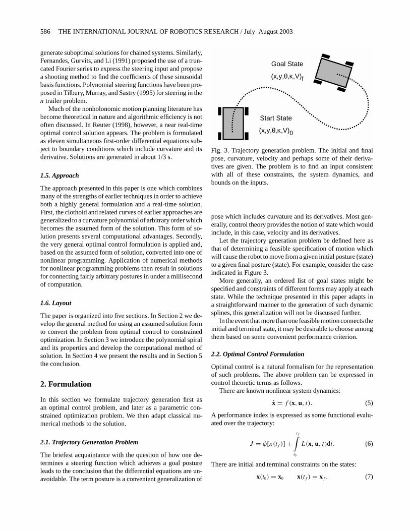
Fig. 3. Trajectory generation problem. The initial and finalpose, curvature, velocity and perhaps some of their deriva-tives are given. The problem is to find an input consistentwith all of these constraints, the system dynamics, andbounds on the inputs.

pose which includes curvature and its derivatives. Most gen-erally, control theory provides the notion of state which wouldinclude, in this case, velocity and its derivatives.

Let the trajectory generation problem be defined here asthat of determining a feasible specification of motion whichwill cause the robot to move from a given initial posture (state)to a given final posture (state). For example, consider the caseindicated in Figure 3.

More generally, an ordered list of goal states might bespecified and constraints of different forms may apply at eachstate. While the technique presented in this paper adapts ina straightforward manner to the generation of such dynamicsplines, this generalization will not be discussed further.

In the event that more than one feasible motion connects theinitial and terminal state, it may be desirable to choose amongthem based on some convenient performance criterion.

2.2. Optimal Control Formulation

Optimal control is a natural formalism for the representationof such problems. The above problem can be expressed incontrol theoretic terms as follows.

There are known nonlinear system dynamics:

x = f (x,u, t). (5)

A performance index is expressed as some functional evalu-ated over the trajectory:

J = φ[x(tf )] +tf∫

t0

L(x,u, t)dt. (6)

There are initial and terminal constraints on the states:

x(t0) = x0 x(tf ) = xf . (7)


There may also be certain pragmatic constraints (reflectingsuch concerns as limited actuator power) on the inputs. Forexample:

|u(t)| ≤ umax(t) |u(t)| ≤ umax(t). (8)

This is a fairly classical formulation of an optimal controlproblem in the Bolza form.

2.3. Constrained Optimization Formulation

Just as the classical technique of variation of parameters con-verts differential equations to algebraic ones, it converts opti-mal control problems to constrained optimization (also knownas nonlinear programming) problems. The technique usedhere is also closely related to the shooting method for bound-ary value problems because an initial guess will be iterativelyrefined based on repeated evaluation of the forward solution.

Parametric representations of solutions are convenientfrom the perspective of the compactness of the representa-tion. When compared with sampled forms of continuous sig-nals, this compactness makes them easier to represent, store,communicate and manipulate. The process of transformationstarts by assuming a solution of the form

u(t) = u(p, t) (9)

where the control is assumed to be a member of a family offunctions which span all possible values of an arbitrary vectorof parametersp of lengthp. An individual control function isnow represented as a point in parameter space.

Since the input completely determines the state, and theparameters now determine the input, dependence on both stateand input is just dependence on the parameters. Accordingly,the state equations can be written as:

x(t) = f[x(p, t),u(p, t), t] = f(p, t). (10)

The state vector would include any variables upon whichboundary conditions are to be imposed as well as any oth-ers upon which these depend.

Let the boundary conditions comprise a set ofn constraintrelations of the form:

h(p, t0, tf ) = x(t0) +tf∫

t0

f(p, t)dt = xb. (11)

It is conventional to write these as:

g(p, t0, tf ) = h(p, t0, tf ) − xb = 0. (12)

Assume there is some scalar performance index which is tobe minimized:

minimize : J (x,u) = φ[x(tf )] +tf∫

t0

L(x,u, t)dt. (13)

Again, because the parameters determine the input which de-termines the state, these expressions can be written as:

minimize : J (p) = φ(p, tf ) +tf∫

t0

L(p, t)dt

subject to: g(p, t0, tf ) = 0 tf free. (14)

It may also be useful to represent the constraint of boundedinputs with something like:

|p| ≤ pmax. (15)

The present problem formulation now looks partially likeoptimal control (due to the integrals) and partially like param-eter optimization. It is now the case that both the state and theperformance index are functions only of the parameters andtime, but the appearance of integrals in both is nontraditional.

2.4. First-Order Dynamic Response to Parameter Variation

The high-level notation masks some severe difficulties in gen-eral. Chief among them is the question of how first derivativeswith respect to the parameters are to be determined. There isgenerally no analytic solution for the state available whichcan be substituted into the equations in order to compute pa-rameter derivatives of the constraintsg(q). Assuming so begsthe original question. Even if the trajectory was available asan integral over the input (as it will be later for polynomialspirals), there is no guarantee that the integrals have closed-form solutions. Hence, implementations generally must relyon numerical methods.

Nonetheless, in order to implement the shooting method,the Jacobians of the performance index and the endpoint withrespect to the parameters will be required. The Leibnitz rulesupplies the principle but the Jacobians can only be extractedindirectly.

The system dynamics can be differentiated with respect tothe parameters to obtain

∂

∂px(t) =

[∂ x∂p

]= F(p, t)

∂x∂p

+ G(p, t)∂u∂p

F = ∂f∂x

G = ∂f∂u

(16)

whereF andG are the Jacobians of the system with respect tothe state and the inputs. Hence, the Jacobian of the state withrespect to the parameters must satisfy the linearized systemdynamics at any point in time. Although there is no solutionto the nonlinear system given in eq. (1), the general solutionto the linearized dynamics (which must exist due to linearity)exists in closed form (Kelly 2001).


Integrating the above gives a self-referential form of theLeibnitz’ rule:

∂x∂p

=tf∫

t0

[F(p, t)

∂x∂p

+ G(p, t)∂u∂p

]dt. (17)

This equation can be integrated to yield the parameter Jaco-bian at the endpoint. Due to the nonlinearity of the equations,a solution would proceed by linearizing the first-order con-ditions. Therefore, second derivatives would be required ingeneral.

In some situations, it is possible to eliminate the self refer-ence to the state to produce a solution integral (a quadrature)which is explicitly of the form:

x(p, tf ) =tf∫

t0

g(p, t)dt. (18)

The Leibnitz rule can be applied directly to this form to getthe parameter Jacobian and the final time gradient:

∂x∂p

=tf∫

t0

[∂g∂p

]dt

∂x∂tf

= g(p, tf ). (19)

Even in this simplified case, however, the parameter Jacobianremains defined by an integral.

Likewise, the performance index can be differentiated:

∂

∂pJ (p) = ∂

∂pφ(p, tf ) (20)

+tf∫

t0

{∂

∂xL(p, t)

∂x∂p

+ ∂

∂uL(p, t)

∂u∂p

}dt.

This information is included here to address how the ap-proach applies to any parametric form of assumed solution.The choice of polynomial spiral will further simplify the cal-culations, but the overall approach can be applied to any formof parametric input.

2.5. Functional Inequality Constraints

Once the constrained optimization formulation is adopted,systematic mechanisms for dealing with inequality con-straints, such as in Kuhn and Tucker (1961) can be broughtto bear. Imposing limits on an input during iteration can beproblematic because such limits apply to the entire time his-tory of the input. Preventing excessive curvature at one timefor example, may cause it somewhere else.

An auxiliary advantage of the present formulation is thatthe maximum value of an input can be approximated by com-

puting itsn-norm

max{ui(t)n} ≈ 1

(tf − t0)

tf∫t0

[ui(t)]ndt (21)

wheren is a large even integer. This expression can now formthe basis of an integral constraint

max{ui(t)n} ≤ (umax)

n (22)

which is no different in principle than the boundary conditionsexcept that it is an inequality.

2.6. Change of Variable

It is often convenient for trajectory generation purposes tochange the independent variable from time to distance. With-out loss of generality, let the initial distance be set to zero.Also, let the final distancesf be absorbed into an adjoinedparameter vector thus:

q = [pT, sf

]T. (23)

The problem formulation under this change of variabletakes the following form:

minimize : J (q) = φ(q) +sf∫

0

L(q)ds

subject to: g(q) = 0 sf free. (24)

2.7. Necessary Conditions

Constrained optimization problems can of course be solved bythe method of Lagrange multipliers. From the theory of con-strained optimization, the solution is obtained by defining theHamiltonian (often called the Lagrangian in the constrainedoptimization context):

H(q,λλλ) = J (q) + λλλTg(q). (25)

The first-order necessary conditions are:

∂

∂qH(q,λλλ) = ∂

∂qJ (q) + λλλT ∂

∂qg(q) = 0T (p + 1 eqns)

∂

∂λλλH(q) = g(q) = 0 (n eqns). (26)

This is a set ofn + p + 1 simultaneous equations in then + p + 1 unknowns inq andλλλ. The equation in the firstset corresponding to the final distance is the transversalitycondition used to determine the final distance in the eventthat it is considered variable. The right-hand side is a rowvector in the first set and a column vector in the second set.


2.8. Methods of Solution

Several numerical techniques are available for the solutionof nonlinear programming problems. The last five chaptersof Luenberger (1989), for example, contain a lucid tutorialon the basic techniques: gradient projection, Lagrange, andpenalty function.

The technique chosen here is a Lagrange method. Suchmethods treat the Lagrange multipliers on an equal footingwith the unknown parameters. The first-order necessary con-ditions are solved directly using multi-dimensional rootfind-ing techniques. Newton’s method is the basis for most of these“curvature” (second derivative) based techniques. As a result,they converge quadratically but must be augmented by mecha-nisms to enhance stability when operating far from a solution.

Newton’s method as it applies to constrained optimizationis derived briefly as follows. Transposing the first set of equa-tions, linearizing about a point where all equations are notsatisfied, and insisting that they become satisfied to first orderafter perturbation gives:

∂2H

∂q2(q,λλλ)�q + ∂

∂qg(q)T�λλλ = − ∂

∂qH(q,λλλ)T (p + 1 eqns)

∂

∂qg(q)�q = −g(q) (n eqns). (27)

Notation for the Hessian of the Hamiltonian (with respect toq) was used:

∂2H

∂q2(q,λλλ) = ∂2J

∂q2(q) + λλλ

∂2

∂q2g(q). (28)

The last term involves a third-order tensor. It can be interpretedas a multiplier weighted sum of the Hessians of each of theindividual constraint equations:

λλλ∂2

∂q2g(q) =

∑i

λi

∂2

∂q2gi(q). (29)

In matrix form, this is now of the form:

∂2H

∂q2(q,λλλ)

∂

∂qg(q)T

∂

∂qg(q) 0

[�q�λλλ

]=

− ∂

∂qH(q,λλλ)T

−g(q)

.

(30)

This matrix equation can be interpreted to provide the er-rors in the parameters which, when added to the parameters,remove the observed residuals to first order. It can be iteratedfrom a good initial guess for the parameters and the multipliersuntil convergence.

It is usually advisable to enforce diagonal dominance inthe manner of the Levenberg–Marquardt algorithm (see Press

1988) in order to enlarge the radius of convergence. Thestructure is also amenable to recursive partitioning (Slama,Theurer, and Henriksen 1980) to improve performance.

Two degenerate forms of the iteration are also importantfor this paper.

2.8.1. Unconstrained Optimization

The degenerate form of unconstrained optimization is of prac-tical significance. In this case, there are no constraint equa-tions and no Lagrange multipliers. Equation (30) degeneratesto the square system[

∂2J

∂q2(q)

]�q = − ∂

∂qJ (q)T (31)

which is the same result that would be obtained by applyingNewton’s method from scratch to this specific problem.

2.8.2. Constraint Satisfaction

The second degenerate form is also of practical significance.Indeed, this is trajectory generation as it was originally posed.Here, there is no objective function. It is simply required thatthe boundary conditions be met. In this case, eq. (30) degen-erates to: [

∂

∂qg(q)

]�q = −g(q). (32)

This is Newton’s method as it occurs in rootfinding contexts.The matrix which appears is the Jacobian of the constraints. Inthis case, it is legitimate for the system to be non-square and,if it is, the appropriate generalized inverse of the Jacobian canbe used in the iteration.

3. Solution Using Polynomial Spirals

The techniques of the previous section will apply to any formof assumed solution. In this section we develop the specificcase when polynomial spirals are the assumed form.

Furthermore, the previous formulation is not confined tosteering functions. It could be used, for example, to determinepolynomials for linear velocity and to enforce accelerationcontinuity. However, such a trivial problem would not requireall of the machinery just presented. Since steering functionsare much harder to determine, in this section we concentrateon this aspect of the problem.

3.1. Achieving Steering Continuity

Even though it is most accurate to consider curvature a state,it is also useful for many purposes to consider curvature tobe an input and to omit the last equation in eq. (1). Underthis assumption, the equations become homogeneous to thefirst degree in linear velocityV (t) and it becomes possible todivide the remaining equations by it in the form of ds/dt to


effect a change of independent variable from time to distance:

d

dsx(s) = cosθ(s)

d

dsy(s) = sinθ(s)

d

dsθ(s) = κ(s). (33)

This form can be most useful for trajectory generation pur-poses because it permits the geometry of the trajectory to beconsidered independent of the speed of traversal.

Under this transformation, and omitting velocity, the end-point constraints in Figure 3 become:

x(s0) = (x0, y0, θ0, κ0)T

x(sf ) = (xf , yf , θf , κf )T. (34)

Of course, if the origin is defined to be positioned atthe initial posture then the first three boundary conditionswill be satisfied by construction and the five constraints[κ0, xf , yf , θf , κf ] would remain to be satisfied in this exam-ple. Five parameters are therefore necessary for generatingsequences of curvature continuous trajectories.

3.2. Clothoids

The clothoid is a well-known curve which is defined by lin-early varying curvature, thus

κ(s) = a + bs. (35)

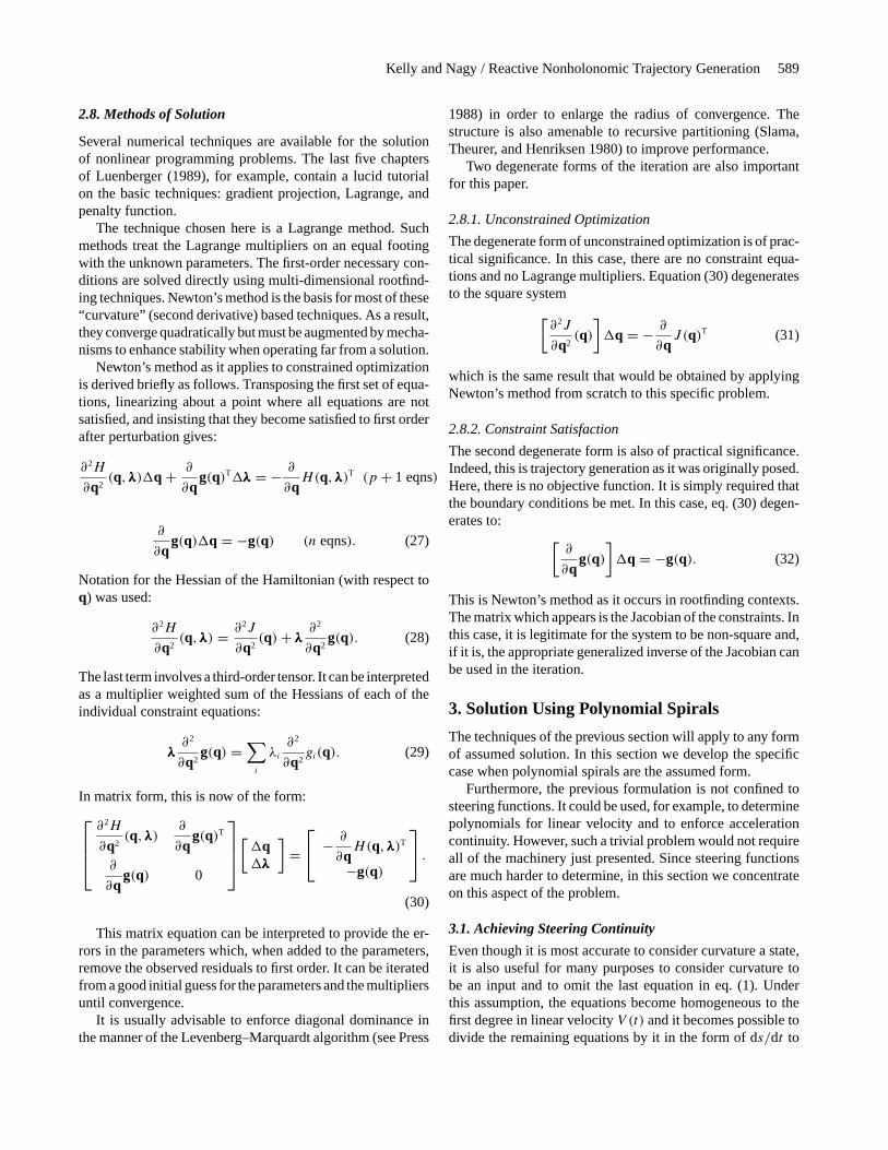
This curve traces out a trajectory inx–y–s space knownas the Cornu spiral (see Figure 4). Of course, with only threeparameters to vary (a, b and s) the clothoid cannot satisfyarbitrary terminal curvature or even heading constraints if theexisting parameters are used to satisfy initial curvature andterminal position.

3.3. Polynomial Spirals

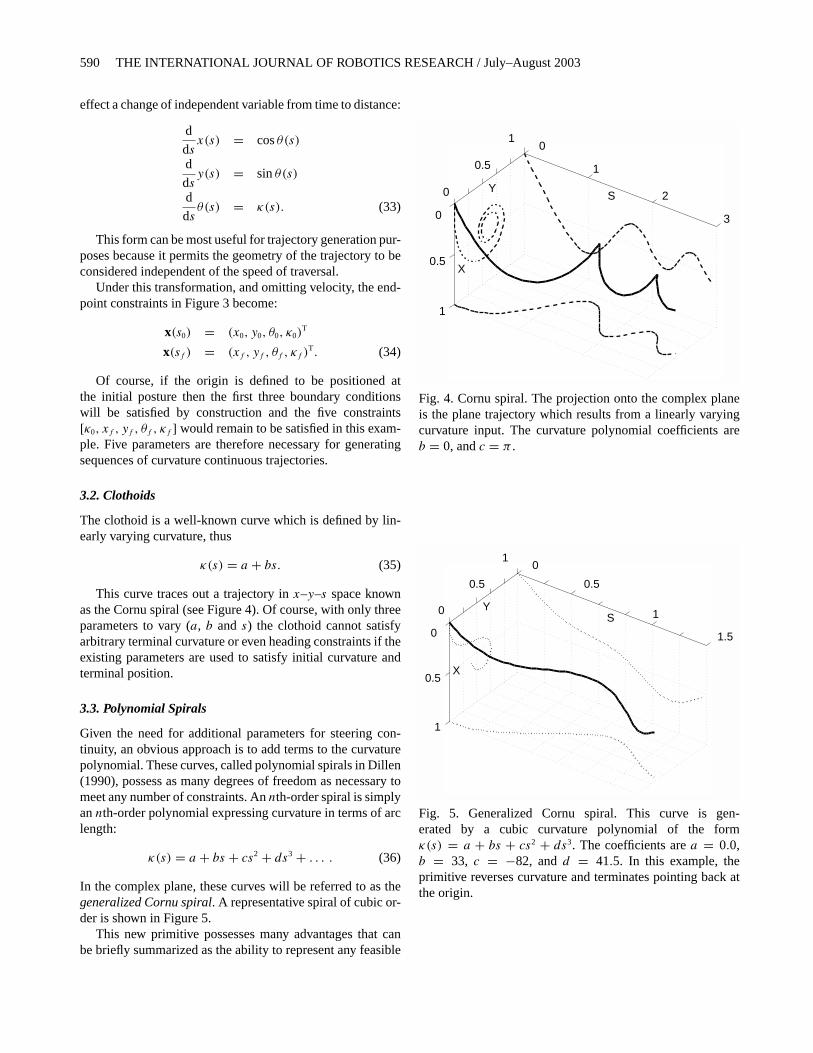
Given the need for additional parameters for steering con-tinuity, an obvious approach is to add terms to the curvaturepolynomial. These curves, called polynomial spirals in Dillen(1990), possess as many degrees of freedom as necessary tomeet any number of constraints. Annth-order spiral is simplyannth-order polynomial expressing curvature in terms of arclength:

κ(s) = a + bs + cs2 + ds3 + . . . . (36)

In the complex plane, these curves will be referred to as thegeneralized Cornu spiral. A representative spiral of cubic or-der is shown in Figure 5.

This new primitive possesses many advantages that canbe briefly summarized as the ability to represent any feasible

S

0

1

2

3

0

0.5

1

0

0.5

1

X

Y

Fig. 4. Cornu spiral. The projection onto the complex planeis the plane trajectory which results from a linearly varyingcurvature input. The curvature polynomial coefficients areb = 0, andc = π .

S

0

0.5

1

1.5

0

0.5

1

0

0.5

1

X

Y

Fig. 5. Generalized Cornu spiral. This curve is gen-erated by a cubic curvature polynomial of the formκ(s) = a + bs + cs2 + ds3. The coefficients area = 0.0,b = 33, c = −82, andd = 41.5. In this example, theprimitive reverses curvature and terminates pointing back atthe origin.


vehicle motion using a small number of parameters. Sucha bold statement is easy to justify by noting that all feasiblemotions have an associated control and the primitive is merelythe Taylor series of the control. The Taylor remainder theoremthen supplies the basis of the claim that all controls can berepresented.

Given that the control in this case represents the actualmotion of the steering actuator, it can also be concluded thathigher-order terms in the series will eventually vanish dueto the impossibly high frequencies that they imply. A smallnumber of parameters is also valuable from the perspectiveof representing and communicating the results, but most im-portantly, it dramatically reduces the dimensionality of thesearch space which is implied in all variational approaches tothe problem.

3.4. Reduction to Decoupled Quadratures

The polynomial spiral has two other important computationaladvantages. Notice that the system dynamics, while coupled,are in echelon form, so that a closed-form solution for headingcould be substituted into the position integrals to decouple thesystem.

The polynomial spiral can be integrated in closed form toproduce heading:

κ(s) = a + bs + cs2 + ds3 + . . .

θ(s) = as + bs2

2+ cs3

3+ ds4

4+ . . . . (37)

The new position integrals then become:

x(s) =s∫

0

cos

[as + bs2

2+ cs3

3+ ds4

4+ . . .

]ds

y(s) =s∫

0

sin

[as + bs2

2+ cs3

3+ ds4

4+ . . .

]ds.(38)

These are the generalized Fresnel integrals. The computa-tion of these transcendental integrals and their gradients withrespect to the parameters will turn out to be the major com-putational burden of trajectory generation.

The main advantage of decoupling is that the first-order be-havior of the system can now also be computed using quadra-ture rather than something like the multidimensional Runge–Kutta required by eq. (17). The parameter Jacobians remaindefined by integrals but at least they are explicit. Their integralnature also leads to an interpretation of eq. (32) as the classicalshooting method for solving boundary value problems.

A second computational advantage is that the state equa-tions become simplified to the maximum degree possiblewhile retaining a fairly general steering function. It is wellknown that the position equations are not solvable in closedform for even a linearly varying heading input (in which case

the integrals are the well-known Fresnel integrals). How-ever, the polynomial spiral has the property that any num-ber of boundary conditions on initial or terminal heading orits derivatives are linear in all parameters but distance. Thismeans that it is straightforward to enforce these conditionsexactly by fixing one parameter in addition to terminal dis-tance and solving the resulting linear equations; only two ofthe equations are ever difficult to solve.

3.5. Boundary Conditions as Constraints

Consider now the expression of the boundary conditions forinitial and terminal posture using polynomial spirals for thecase of enforcing curvature continuity. This case correspondsto cubic polynomials and five parameters:

κ(s) = a + bs + cs2 + ds3. (39)

The initial constraints on position and heading can be satisfiedtrivially by choosing coordinates such that:

s0 = 0 x(0) = y(0) = θ(0) = 0. (40)

This leaves constraints on initial curvature and its derivativesas well as the entire final posture to be satisfied. We define thevector of polynomial spiral parameters to be the coefficients:

q = [a b c d sf

]T. (41)

The initial curvature is satisfied trivially:

a = κ(0) (42)

and any higher-order initial derivatives in a more general casecould be resolved similarly. To save computation, this pa-rameter will be eliminated from the iterative equations. Theremaining constraint equations in standard form are therefore:

g(q) = h(q) − xb = 0 or

h1(q) − xf = 0h2(q) − yf = 0h3(q) − θf = 0h4(q) − κf = 0

. (43)

The equations for terminal curvatureκf and headingθf arepolynomials while the endpoint constraintsxf and yf arequadratures. The Jacobian matrix of the above nonlinear sys-tem is just a top to bottom arrangement of the gradients ofeach constraint:

∂g∂q

= ∂h∂q

=

∂x

∂b

∂x

∂c

∂x

∂d. . .

∂x

∂sf. . . . . . . . . . . . . . .∂κ

∂b

∂κ

∂c

∂κ

∂d. . .

∂κ

∂sf

. (44)

For the position coordinates, the Leibnitz’ rule can be used tocompute the derivatives. Details of a Simpson’s rule imple-mentation for computing these functions and their first andsecond derivatives are provided in the Appendix.


3.6. Boundary Conditions as Performance Indices

It is also valid and may be convenient to formulate the bound-ary conditions as costs rather than hard constraints. Let theterminal error be scaled as follows:

�x(q) =

x(q) − xf

y(q) − yf

L[θ(q) − θf ]L2[κ(q) − κf ]

. (45)

The characteristic lengthL is used to make the units of eachelement of the vector consistent and to make each element ofroughly equal significance. A useful interpretation is that theheading and curvature error are being converted to their effecton the position of a point a distanceL away. For the forktruckapplication, for example,L could be set to the sum of thelength of the forks and the distance the vehicle will travel toinsert them. The absolute bounds on this terminal error aredenoted as:

�xmax = [�xmax�ymax�θmax�κmax ]T . (46)

An associated performance index could then given by thesquared terminal error:

φ(q) = 1

2

[�x(q)

]T [�x(q)]. (47)

The gradient of the performance index with respect to theparameters is the sum of several components:

∂φ

∂q=

[∂x

∂q�x + ∂y

∂q�y + L2 ∂θ

∂q�θ + L4 ∂κ

∂q�κ

]. (48)

Here, the vectors∂x/∂q, etc., are the gradients (row vectors)of the terminal posture with respect to the parameters. TheHessian matrix is computed by differentiating this:

∂2

∂q2(φ) =

[∂2x

∂q2�x + ∂2y

∂q2�y + L2 ∂

2θ

∂q2�θ + L4 ∂

2κ

∂q2�κ

+ ∂xT

∂q∂x

∂q+ ∂yT

∂q∂y

∂q+ L2 ∂θ

T

∂q∂θ

∂q+ L4 ∂κ

T

∂q∂κ

∂q

].

(49)

The last four terms involve outer product (hence symmetric)matrices formed by multiplying individual gradients by theirtransposes. These outer products can be evaluated numericallygiven the gradients. When near a solution, these outer productterms dominate the Hessian.

3.7. Smoothness as a Performance Index

It is also possible to create a performance index which preferssmooth trajectories. In this case, an integral form is appro-priate. The following functional form will discourage highcurvature values relative to more graceful turns:

Jκ(q) = 1

2

sf∫0

[κ(q)]2ds. (50)

Terms involving heading or curvature derivatives could also beadded to discourage indirect routes or rapid steering changes.Note that wheneverq appears inside a distance integral, theterminal arc lengthsf should be interpreted as the variable ofintegrations.

The gradient of the performance index with respect to theparameters is obtained from the Leibnitz’ rule:

∂Jκ

∂q=

sf∫0

κ(q)∂κ

∂qds. (51)

The Hessian matrix is computed by differentiating this:

∂2

∂q2(Jκ) =

sf∫0

[∂κT

∂q∂κ

∂q+ κ(q)

∂2κ

∂q2

]ds. (52)

The previous performance index could also be added to thisone in order to produce smooth trajectories which almost meetthe constraints in some optimum fashion.

4. Results

In this section we present some numerical validations of theapproach to trajectory generation.

4.1. Forward Problem

A good solution to the forward problem for the boundary con-ditions and their derivatives is necessary because it becomesthe basis for solving the more difficult inverse problem. Ofcourse, only the position coordinates present any difficulty.

In the present implementation, Simpson’s rule is used toperform all of the integrations numerically. Many of the in-tegrands are quite smooth and can often be estimated wellnumerically in as little as ten integrand evaluations. In thiscontext, “estimated well” means well enough to determineend posture to perhaps a few millimeters in position and afew milliradians in heading.

When coefficients are large in magnitude, it may be nec-essary to perform many integrand evaluations in Simpson’srule. At some point, large coefficients correspond to infea-sible inputs and the difficulty in computation indicates dif-ficulty or even impossibility of execution. In rough terms,curves that cannot be computed, cannot be executed anyway.The appendix provides a straightforward mechanism to reusecomputations while refining the estimate of the quadratures.

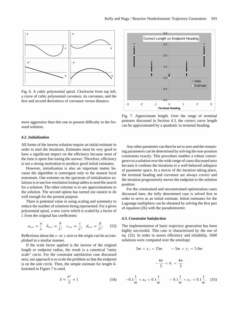
Figure 6 shows a typical member of the cubic curvaturepolynomial family of curves computed. Curves must be much


s

ss

κ

κ’

x

y

κ’’

Fig. 6. A cubic polynomial spiral. Clockwise from top left,a curve of cubic polynomial curvature, its curvature, and thefirst and second derivatives of curvature versus distance.

more aggressive than this one to present difficulty in the for-ward solution.

4.2. Initialization

All forms of the inverse solution require an initial estimate inorder to start the iterations. Estimates must be very good tohave a significant impact on the efficiency because most ofthe time is spent fine tuning the answer. Therefore, efficiencyis not a strong motivation to produce good initial estimates.

However, initialization is also an important matter be-cause the algorithm is convergent only to the nearest localextremum. One extreme on the spectrum of initialization so-lutions is to use low resolution lookup tables to seed the searchfor a solution. The other extreme is to use approximations tothe solution. The second option has turned out easiest to dowell enough for the present purpose.

There is potential value in using scaling and symmetry toreduce the number of solutions being represented. For a givenpolynomial spiral, a new curve which is scaled by a factor ofλ from the original has coefficients:

anew = a

λbnew = b

λ2cnew = c

λ3dnew = d

λ4. (53)

Reflections about thex- or y-axis or the origin can be accom-plished in a similar manner.

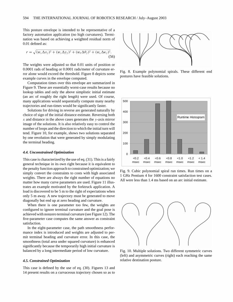
If the scale factor applied is the inverse of the originallength or endpoint radius, the result is a canonical “unityscale” curve. For the constraint satisfaction case discussednext, our approach is to scale the problem so that the endpointis on the unit circle. Then, the simple estimate for length il-lustrated in Figure 7 is used.

S ≈ θ2

5+ 1 (54)

Correct Length vs Endpoint Heading

0.0

0.5

1.0

1.5

2.0

2.5

3.0

-3 -2 -1 0 1 2 3Terminal Heading

DataEstimate

Fig. 7. Approximate length. Over the range of terminalpostures discussed in Section 4.3, the correct curve lengthcan be approximated by a quadratic in terminal heading.

Any other parameter can then be set to zero and the remain-ing parameters can be determined by solving the non-positionconstraints exactly. This procedure enables a robust conver-gence to a solution over the wide range of cases discussed nextbecause it confines the iterations to a well-behaved subspaceof parameter space. In a movie of the iteration taking place,the terminal heading and curvature are always correct andthe iteration progressively moves the endpoint to the solutionposition.

For the constrained and unconstrained optimization casesdiscussed later, the fully determined case is solved first inorder to serve as an initial estimate. Initial estimates for theLagrange multipliers can be obtained by solving the first partof equation (26) with the pseudoinverter.

4.3. Constraint Satisfaction

The implementation of basic trajectory generation has beenhighly successful. This case is characterized by the use ofeq. (32). In order to assess efficiency and reliability, 1600solutions were computed over the envelope:

5m < xf < 15m − 5m < yf < 5.0m

−4π

5< θf <

4π

5

−0.11

m< κ0 < 0.1

1

m− 0.1

1

m< κf < 0.1

1

m. (55)


This posture envelope is intended to be representative of afactory automation application (no high curvatures). Termi-nation was based on achieving a weighted residual norm of0.01 defined as:

r = √(wx�xf )2 + (wy�yf )2 + (wθ�θf )2 + (wκ�κf )2.

(56)

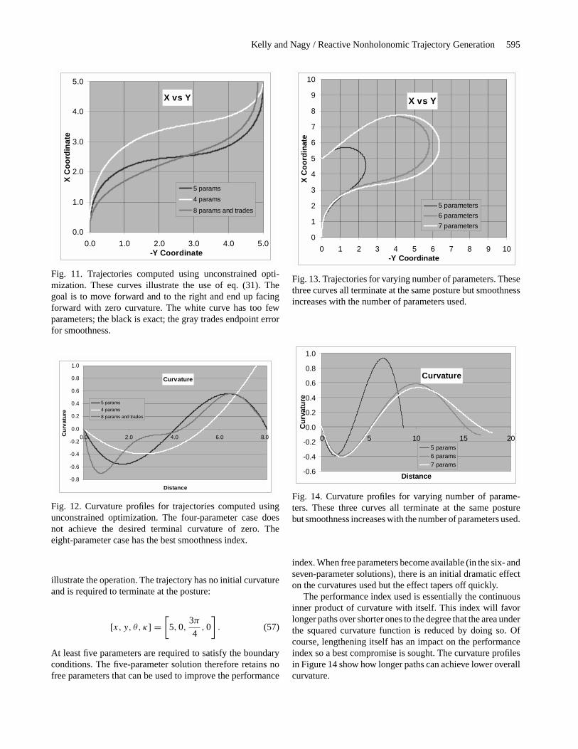
The weights were adjusted so that 0.01 units of position or0.0001 rads of heading or 0.0001 rads/meter of curvature er-ror alone would exceed the threshold. Figure 8 depicts someexample curves in the envelope computed.

Computation times over this envelope are summarized inFigure 9. These are essentially worst-case results because nolookup tables and only the above simplistic initial estimate(an arc of roughly the right length) were used. Of course,many applications would sequentially compute many nearbytrajectories and run-times would be significantly faster.

Solutions for driving in reverse are generated naturally bychoice of sign of the initial distance estimate. Reversing bothx and distance in the above cases generates they-axis mirrorimage of the solutions. It is also relatively easy to control thenumber of loops and the direction to which the initial turn willtend. Figure 10, for example, shows two solutions separatedby one revolution that were generated by simply modulatingthe terminal heading.

4.4. Unconstrained Optimization

This case is characterized by the use of eq. (31). This is a fairlygeneral technique in its own right because it is equivalent tothe penalty function approach to constrained optimization; wesimply convert the constraints to costs with high associatedweights. There are always the right number of equations nomatter how many curve parameters are used. Figure 11 illus-trates an example motivated by the forktruck application. Aload is discovered to be 5 m to theright of expectations whenonly 5 m away. A newtrajectory must be generated to movediagonally but end up at zero heading and curvature.

When there is one parameter too few, the weights areconfigured to ignore terminal curvature and the goal pose isachieved with nonzero terminal curvature (see Figure 12). Thefive-parameter case computes the same answer as constraintsatisfaction.

In the eight-parameter case, the path smoothness perfor-mance index is introduced and weights are adjusted to per-mit terminal heading and curvature error. In this case, thesmoothness (total area under squared curvature) is enhancedsignificantly because the temporarily high initial curvature isbalanced by a long intermediate period of low curvature.

4.5. Constrained Optimization

This case is defined by the use of eq. (30). Figures 13 and14 present results on a curvaceous trajectory chosen so as to

Fig. 8. Example polynomial spirals. These different endpostures have feasible solutions.

Runtime Histogram

0

100

200

300

400

500

<0.2msec

<0.4msec

<0.6msec

<0.8msec

<1.0msec

<1.2msec

< 1.4msec

Fig. 9. Cubic polynomial spiral run times. Run times on a1 GHz Pentium 4 for 1600 constraint satisfaction test cases.All were less than 1.4 ms based on an arc initial estimate.

Fig. 10. Multiple solutions. Two different symmetric curves(left) and asymmetric curves (right) each reaching the samerelative destination posture.


X vs Y

0.0

1.0

2.0

3.0

4.0

5.0

0.0 1.0 2.0 3.0 4.0 5.0-Y Coordinate

X C

oord

inat

e

5 params

4 params

8 params and trades

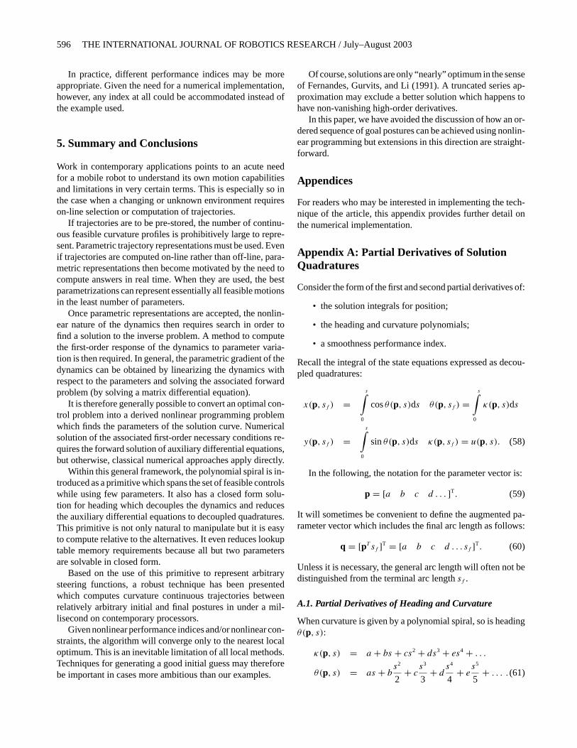
Fig. 11. Trajectories computed using unconstrained opti-mization. These curves illustrate the use of eq. (31). Thegoal is to move forward and to the right and end up facingforward with zero curvature. The white curve has too fewparameters; the black is exact; the gray trades endpoint errorfor smoothness.

Curvature

-0.8

-0.6

-0.4

-0.2

0.0

0.2

0.4

0.6

0.8

1.0

0.0 2.0 4.0 6.0 8.0

Distance

Cur

vatu

re

5 params

4 params

8 params and trades

Fig. 12. Curvature profiles for trajectories computed usingunconstrained optimization. The four-parameter case doesnot achieve the desired terminal curvature of zero. Theeight-parameter case has the best smoothness index.

illustrate the operation. The trajectory has no initial curvatureand is required to terminate at the posture:

[x, y, θ, κ] =[5,0,

3π

4,0

]. (57)

At least five parameters are required to satisfy the boundaryconditions. The five-parameter solution therefore retains nofree parameters that can be used to improve the performance

X vs Y

0

1

2

3

4

5

6

7

8

9

10

0 1 2 3 4 5 6 7 8 9 10-Y Coordinate

X C

oord

inat

e

5 parameters

6 parameters

7 parameters

Fig. 13. Trajectories for varying number of parameters. Thesethree curves all terminate at the same posture but smoothnessincreases with the number of parameters used.

Curvature

-0.6

-0.4

-0.2

0.0

0.2

0.4

0.6

0.8

1.0

0 5 10 15 20

Distance

Cur

vatu

re

5 params6 params7 params

Fig. 14. Curvature profiles for varying number of parame-ters. These three curves all terminate at the same posturebut smoothness increases with the number of parameters used.

index. When free parameters become available (in the six- andseven-parameter solutions), there is an initial dramatic effecton the curvatures used but the effect tapers off quickly.

The performance index used is essentially the continuousinner product of curvature with itself. This index will favorlonger paths over shorter ones to the degree that the area underthe squared curvature function is reduced by doing so. Ofcourse, lengthening itself has an impact on the performanceindex so a best compromise is sought. The curvature profilesin Figure 14 show how longer paths can achieve lower overallcurvature.


In practice, different performance indices may be moreappropriate. Given the need for a numerical implementation,however, any index at all could be accommodated instead ofthe example used.

5. Summary and Conclusions

Work in contemporary applications points to an acute needfor a mobile robot to understand its own motion capabilitiesand limitations in very certain terms. This is especially so inthe case when a changing or unknown environment requireson-line selection or computation of trajectories.

If trajectories are to be pre-stored, the number of continu-ous feasible curvature profiles is prohibitively large to repre-sent. Parametric trajectory representations must be used. Evenif trajectories are computed on-line rather than off-line, para-metric representations then become motivated by the need tocompute answers in real time. When they are used, the bestparametrizations can represent essentially all feasible motionsin the least number of parameters.

Once parametric representations are accepted, the nonlin-ear nature of the dynamics then requires search in order tofind a solution to the inverse problem. A method to computethe first-order response of the dynamics to parameter varia-tion is then required. In general, the parametric gradient of thedynamics can be obtained by linearizing the dynamics withrespect to the parameters and solving the associated forwardproblem (by solving a matrix differential equation).

It is therefore generally possible to convert an optimal con-trol problem into a derived nonlinear programming problemwhich finds the parameters of the solution curve. Numericalsolution of the associated first-order necessary conditions re-quires the forward solution of auxiliary differential equations,but otherwise, classical numerical approaches apply directly.

Within this general framework, the polynomial spiral is in-troduced as a primitive which spans the set of feasible controlswhile using few parameters. It also has a closed form solu-tion for heading which decouples the dynamics and reducesthe auxiliary differential equations to decoupled quadratures.This primitive is not only natural to manipulate but it is easyto compute relative to the alternatives. It even reduces lookuptable memory requirements because all but two parametersare solvable in closed form.

Based on the use of this primitive to represent arbitrarysteering functions, a robust technique has been presentedwhich computes curvature continuous trajectories betweenrelatively arbitrary initial and final postures in under a mil-lisecond on contemporary processors.

Given nonlinear performance indices and/or nonlinear con-straints, the algorithm will converge only to the nearest localoptimum. This is an inevitable limitation of all local methods.Techniques for generating a good initial guess may thereforebe important in cases more ambitious than our examples.

Of course, solutions are only “nearly” optimum in the senseof Fernandes, Gurvits, and Li (1991). A truncated series ap-proximation may exclude a better solution which happens tohave non-vanishing high-order derivatives.

In this paper, we have avoided the discussion of how an or-dered sequence of goal postures can be achieved using nonlin-ear programming but extensions in this direction are straight-forward.

Appendices

For readers who may be interested in implementing the tech-nique of the article, this appendix provides further detail onthe numerical implementation.

Appendix A: Partial Derivatives of SolutionQuadratures

Consider the form of the first and second partial derivatives of:

• the solution integrals for position;

• the heading and curvature polynomials;

• a smoothness performance index.

Recall the integral of the state equations expressed as decou-pled quadratures:

x(p, sf ) =s∫

0

cosθ(p, s)ds θ(p, sf ) =s∫

0

κ(p, s)ds

y(p, sf ) =s∫

0

sinθ(p, s)ds κ(p, sf ) = u(p, s). (58)

In the following, the notation for the parameter vector is:

p = [a b c d . . . ]T. (59)

It will sometimes be convenient to define the augmented pa-rameter vector which includes the final arc length as follows:

q = [pT sf ]T = [a b c d . . . sf ]T. (60)

Unless it is necessary, the general arc length will often not bedistinguished from the terminal arc lengthsf .

A.1. Partial Derivatives of Heading and Curvature

When curvature is given by a polynomial spiral, so is headingθ(p, s):

κ(p, s) = a + bs + cs2 + ds3 + es4 + . . .

θ(p, s) = as + bs2

2+ c

s3

3+ d

s4

4+ e

s5

5+ . . . . (61)


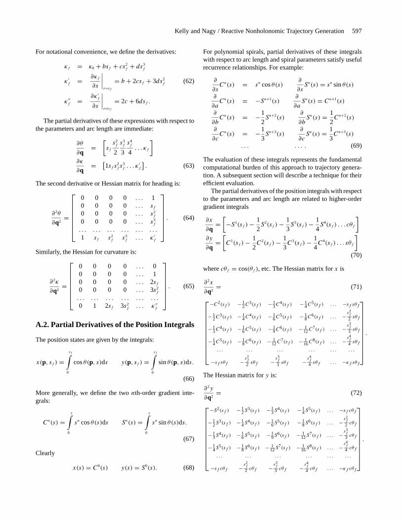
For notational convenience, we define the derivatives:

κf = κ0 + bsf + cs2f

+ ds3f

κ ′f

= ∂κf

∂s

∣∣∣∣s=sf

= b + 2csf + 3ds2f

(62)

κ ′′f

= ∂κ ′f

∂s

∣∣∣∣s=sf

= 2c + 6dsf .

The partial derivatives of these expressions with respect tothe parameters and arc length are immediate:

∂θ

∂q=

[sfs2f

2

s3f

3

s4f

4. . . κf

]∂κ

∂q= [

1sf s2fs3f. . . κ ′

f

]. (63)

The second derivative or Hessian matrix for heading is:

∂2θ

∂q2=

0 0 0 0 . . . 10 0 0 0 . . . sf0 0 0 0 . . . s2

f

0 0 0 0 . . . s3f

. . . . . . . . . . . . . . . . . .

1 sf s2f

s3f

. . . κ ′f

. (64)

Similarly, the Hessian for curvature is:

∂2κ

∂q2=

0 0 0 0 . . . 00 0 0 0 . . . 10 0 0 0 . . . 2sf0 0 0 0 . . . 3s2

f

. . . . . . . . . . . . . . . . . .

0 1 2sf 3s2f

. . . κ ′′f

. (65)

A.2. Partial Derivatives of the Position Integrals

The position states are given by the integrals:

x(p, sf ) =sf∫

0

cosθ(p, s)ds y(p, sf ) =sf∫

0

sinθ(p, s)ds.

(66)

More generally, we define the twonth-order gradient inte-grals:

Cn(s) =s∫

0

sn cosθ(s)ds Sn(s) =s∫

0

sn sinθ(s)ds.

(67)

Clearly

x(s) = C0(s) y(s) = S0(s). (68)

For polynomial spirals, partial derivatives of these integralswith respect to arc length and spiral parameters satisfy usefulrecurrence relationships. For example:

∂

∂sCn(s) = sn cosθ(s)

∂

∂sSn(s) = sn sinθ(s)

∂

∂aCn(s) = −Sn+1(s)

∂

∂aSn(s) = Cn+1(s)

∂

∂bCn(s) = −1

2Sn+2(s)

∂

∂bSn(s) = 1

2Cn+2(s)

∂

∂cCn(s) = −1

3Sn+3(s)

∂

∂cSn(s) = 1

3Cn+3(s)

. . . . . . . (69)

The evaluation of these integrals represents the fundamentalcomputational burden of this approach to trajectory genera-tion. A subsequent section will describe a technique for theirefficient evaluation.

The partial derivatives of the position integrals with respectto the parameters and arc length are related to higher-ordergradient integrals

∂x

∂q=

[−S1(sf ) − 1

2S2(sf ) − 1

3S3(sf ) − 1

4S4(sf ) . . . cθf

]∂y

∂q=

[C1(sf ) − 1

2C2(sf ) − 1

3C3(sf ) − 1

4C4(sf ) . . . sθf

](70)

wherecθf = cos(θf ), etc. The Hessian matrix forx is

∂2x

∂q2= (71)

−C2(sf ) − 12C

3(sf ) − 13C

4(sf ) − 14C

5(sf ) . . . −sf sθf

− 12C

3(sf ) − 14C

4(sf ) − 16C

5(sf ) − 18C

6(sf ) . . . − s2f

2 sθf

− 13C

4(sf ) − 16C

5(sf ) − 19C

6(sf ) − 112C

7(sf ) . . . − s3f

3 sθf

− 14C

5(sf ) − 18C

6(sf ) − 112C

7(sf ) − 116C

8(sf ) . . . − s4f

4 sθf

. . . . . . . . . . . . . . . . . .

−sf sθf − s2f

2 sθf − s3f

3 sθf − s4f

4 sθf . . . −κf sθf

.

The Hessian matrix fory is:

∂2y

∂q2= (72)

−S2(sf ) − 12S

3(sf ) − 13S

4(sf ) − 14S

5(sf ) . . . −sf cθf

− 12S

3(sf ) − 14S

4(sf ) − 16S

5(sf ) − 18S

6(sf ) . . . − s2f

2 cθf

− 13S

4(sf ) − 16S

5(sf ) − 19S

6(sf ) − 112S

7(sf ) . . . − s3f

3 cθf

− 14S

5(sf ) − 18S

6(sf ) − 112S

7(sf ) − 116S

8(sf ) . . . − s4f

4 cθf

. . . . . . . . . . . . . . . . . .

−sf cθf − s2f

2 cθf − s3f

3 cθf − s4f

4 cθf . . . −κf cθf

.


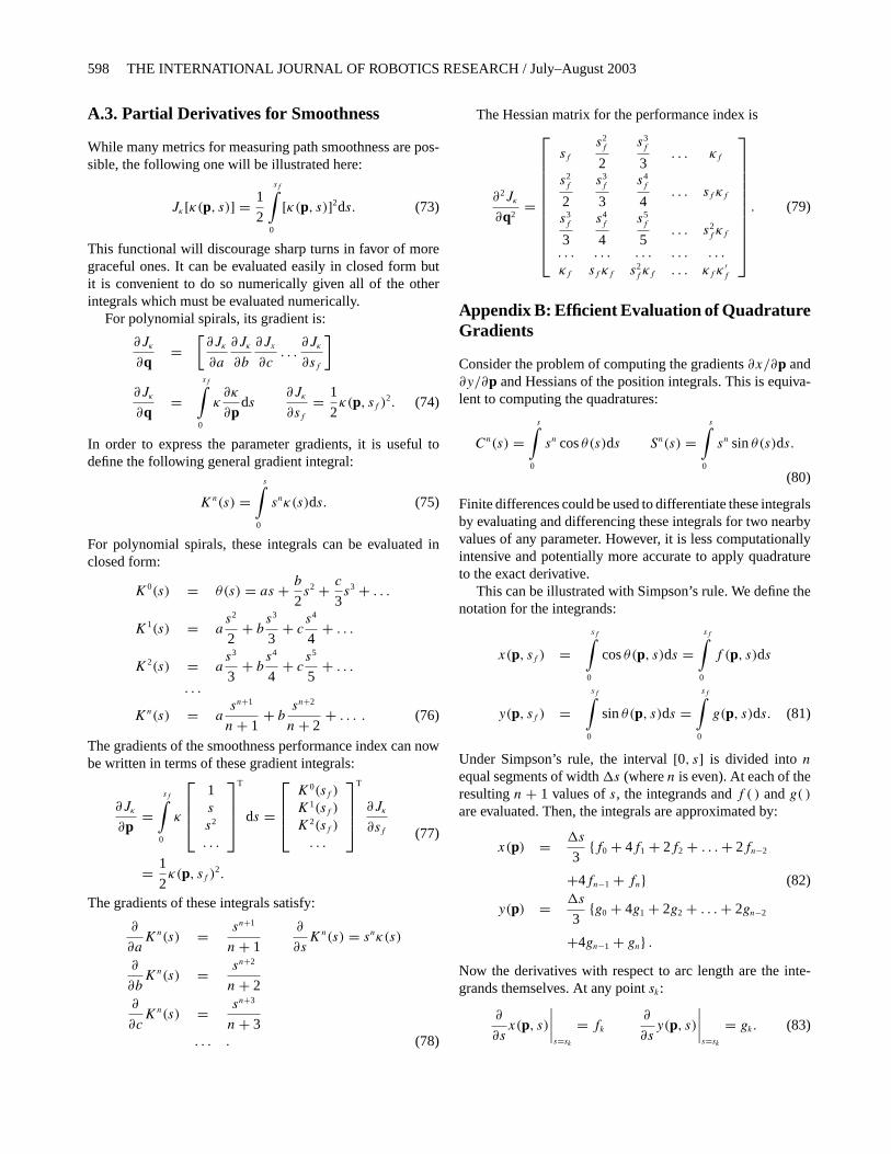
A.3. Partial Derivatives for Smoothness

While many metrics for measuring path smoothness are pos-sible, the following one will be illustrated here:

Jκ[κ(p, s)] = 1

2

sf∫0

[κ(p, s)]2ds. (73)

This functional will discourage sharp turns in favor of moregraceful ones. It can be evaluated easily in closed form butit is convenient to do so numerically given all of the otherintegrals which must be evaluated numerically.

For polynomial spirals, its gradient is:

∂Jκ

∂q=

[∂Jκ

∂a

∂Jκ

∂b

∂Jx

∂c. . .

∂Jκ

∂sf

]

∂Jκ

∂q=

sf∫0

κ∂κ

∂pds

∂Jκ

∂sf= 1

2κ(p, sf )2. (74)

In order to express the parameter gradients, it is useful todefine the following general gradient integral:

Kn(s) =s∫

0

snκ(s)ds. (75)

For polynomial spirals, these integrals can be evaluated inclosed form:

K0(s) = θ(s) = as + b

2s2 + c

3s3 + . . .

K1(s) = as2

2+ b

s3

3+ c

s4

4+ . . .

K2(s) = as3

3+ b

s4

4+ c

s5

5+ . . .

. . .

Kn(s) = asn+1

n + 1+ b

sn+2

n + 2+ . . . . (76)

The gradients of the smoothness performance index can nowbe written in terms of these gradient integrals:

∂Jκ

∂p=

sf∫0

κ

1s

s2

. . .

T

ds =

K0(sf )

K1(sf )

K2(sf )

. . .

T

∂Jκ

∂sf

= 1

2κ(p, sf )2.

(77)

The gradients of these integrals satisfy:

∂

∂aKn(s) = sn+1

n + 1

∂

∂sKn(s) = snκ(s)

∂

∂bKn(s) = sn+2

n + 2∂

∂cKn(s) = sn+3

n + 3. . . . (78)

The Hessian matrix for the performance index is

∂2Jκ

∂q2=

sfs2f

2

s3f

3. . . κf

s2f

2

s3f

3

s4f

4. . . sf κf

s3f

3

s4f

4

s5f

5. . . s2

fκf

. . . . . . . . . . . . . . .

κf sf κf s2fκf . . . κf κ

′f

. (79)

Appendix B: Efficient Evaluation of QuadratureGradients

Consider the problem of computing the gradients∂x/∂p and∂y/∂p and Hessians of the position integrals. This is equiva-lent to computing the quadratures:

Cn(s) =s∫

0

sn cosθ(s)ds Sn(s) =s∫

0

sn sinθ(s)ds.

(80)

Finite differences could be used to differentiate these integralsby evaluating and differencing these integrals for two nearbyvalues of any parameter. However, it is less computationallyintensive and potentially more accurate to apply quadratureto the exact derivative.

This can be illustrated with Simpson’s rule. We define thenotation for the integrands:

x(p, sf ) =sf∫

0

cosθ(p, s)ds =sf∫

0

f (p, s)ds

y(p, sf ) =sf∫

0

sinθ(p, s)ds =sf∫

0

g(p, s)ds. (81)

Under Simpson’s rule, the interval[0, s] is divided intonequal segments of width�s (wheren is even). At each of theresultingn + 1 values ofs, the integrands andf ( ) andg( )are evaluated. Then, the integrals are approximated by:

x(p) = �s

3{f0 + 4f1 + 2f2 + . . . + 2fn−2

+4fn−1 + fn} (82)

y(p) = �s

3{g0 + 4g1 + 2g2 + . . . + 2gn−2

+4gn−1 + gn} .Now the derivatives with respect to arc length are the inte-grands themselves. At any pointsk:

∂

∂sx(p, s)

∣∣∣∣s=sk

= fk

∂

∂sy(p, s)

∣∣∣∣s=sk

= gk. (83)


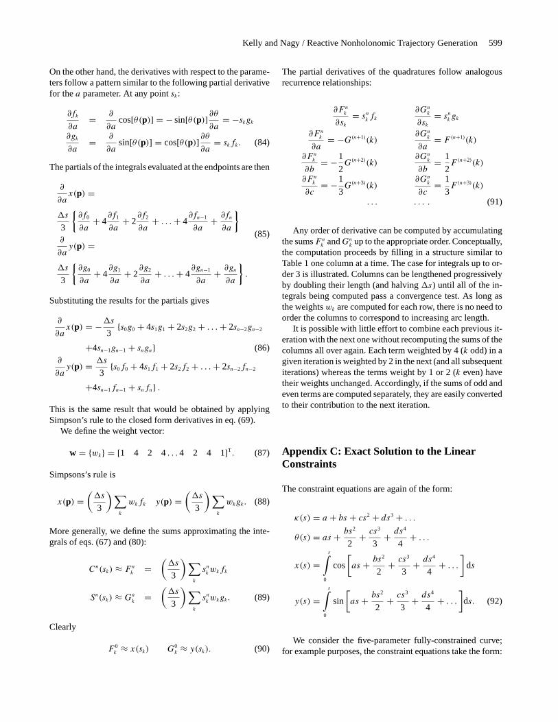
On the other hand, the derivatives with respect to the parame-ters follow a pattern similar to the following partial derivativefor thea parameter. At any pointsk:

∂fk

∂a= ∂

∂acos[θ(p)] = − sin[θ(p)]∂θ

∂a= −skgk

∂gk

∂a= ∂

∂asin[θ(p)] = cos[θ(p)]∂θ

∂a= skfk. (84)

The partials of the integrals evaluated at the endpoints are then

∂

∂ax(p) =

�s

3

{∂f0

∂a+ 4

∂f1

∂a+ 2

∂f2

∂a+ . . . + 4

∂fn−1

∂a+ ∂fn

∂a

}∂

∂ay(p) =

�s

3

{∂g0

∂a+ 4

∂g1

∂a+ 2

∂g2

∂a+ . . . + 4

∂gn−1

∂a+ ∂gn

∂a

}.

(85)

Substituting the results for the partials gives

∂

∂ax(p) = −�s

3{s0g0 + 4s1g1 + 2s2g2 + . . . + 2sn−2gn−2

+4sn−1gn−1 + sngn} (86)∂

∂ay(p) = �s

3{s0f0 + 4s1f1 + 2s2f2 + . . . + 2sn−2fn−2

+4sn−1fn−1 + snfn} .

This is the same result that would be obtained by applyingSimpson’s rule to the closed form derivatives in eq. (69).

We define the weight vector:

w = {wk} = [1 4 2 4. . .4 2 4 1]T. (87)

Simpsons’s rule is

x(p) =(�s

3

) ∑k

wkfk y(p) =(�s

3

) ∑k

wkgk. (88)

More generally, we define the sums approximating the inte-grals of eqs. (67) and (80):

Cn(sk) ≈ Fn

k=

(�s

3

) ∑k

snkwkfk

Sn(sk) ≈ Gn

k=

(�s

3

) ∑k

snkwkgk. (89)

Clearly

F 0k

≈ x(sk) G0k≈ y(sk). (90)

The partial derivatives of the quadratures follow analogousrecurrence relationships:

∂F nk

∂sk= sn

kfk

∂Gnk

∂sk= sn

kgk

∂F nk

∂a= −G(n+1)(k)

∂Gnk

∂a= F (n+1)(k)

∂F nk

∂b= −1

2G(n+2)(k)

∂Gnk

∂b= 1

2F (n+2)(k)

∂F nk

∂c= −1

3G(n+3)(k)

∂Gnk

∂c= 1

3F (n+3)(k)

. . . . . . . (91)

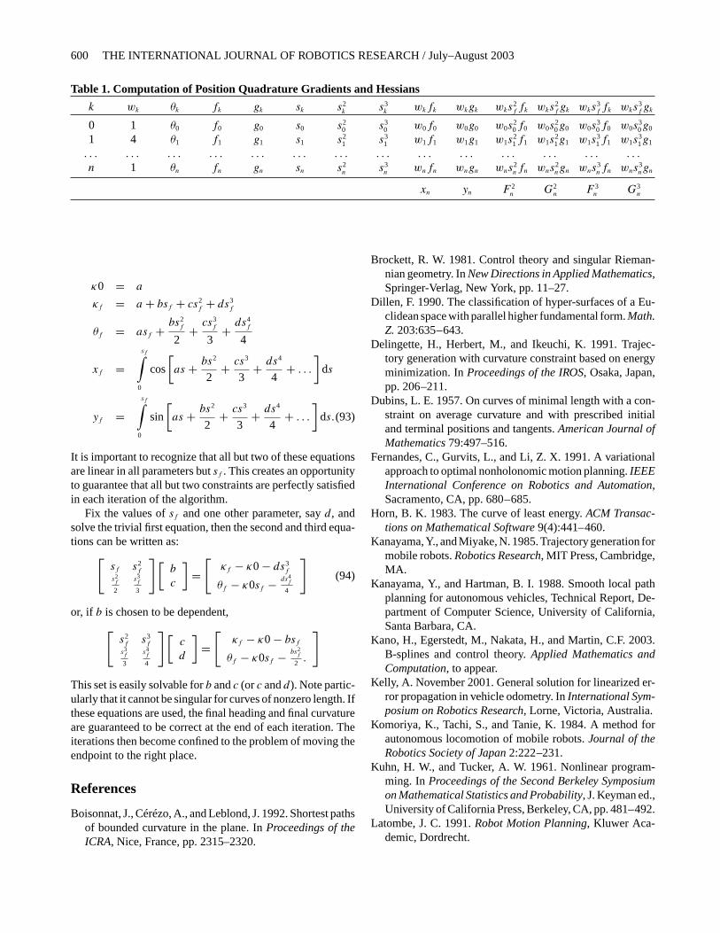
Any order of derivative can be computed by accumulatingthe sumsFn

kandGn

kup to the appropriate order. Conceptually,

the computation proceeds by filling in a structure similar toTable 1 one column at a time. The case for integrals up to or-der 3 is illustrated. Columns can be lengthened progressivelyby doubling their length (and halving�s) until all of the in-tegrals being computed pass a convergence test. As long asthe weightswk are computed for each row, there is no need toorder the columns to correspond to increasing arc length.

It is possible with little effort to combine each previous it-eration with the next one without recomputing the sums of thecolumns all over again. Each term weighted by 4 (k odd) in agiven iteration is weighted by 2 in the next (and all subsequentiterations) whereas the terms weight by 1 or 2 (k even) havetheir weights unchanged. Accordingly, if the sums of odd andeven terms are computed separately, they are easily convertedto their contribution to the next iteration.

Appendix C: Exact Solution to the LinearConstraints

The constraint equations are again of the form:

κ(s) = a + bs + cs2 + ds3 + . . .

θ(s) = as + bs2

2+ cs3

3+ ds4

4+ . . .

x(s) =s∫

0

cos

[as + bs2

2+ cs3

3+ ds4

4+ . . .

]ds

y(s) =s∫

0

sin

[as + bs2

2+ cs3

3+ ds4

4+ . . .

]ds. (92)

We consider the five-parameter fully-constrained curve;for example purposes, the constraint equations take the form:


Table 1. Computation of Position Quadrature Gradients and Hessians

k wk θk fk gk sk s2k

s3k

wkfk wkgk wks2ffk wks

2fgk wks

3ffk wks

3fgk

0 1 θ0 f0 g0 s0 s20 s3

0 w0f0 w0g0 w0s20f0 w0s

20g0 w0s

30f0 w0s

30g0

1 4 θ1 f1 g1 s1 s21 s3

1 w1f1 w1g1 w1s21f1 w1s

21g1 w1s

31f1 w1s

31g1

. . . . . . . . . . . . . . . . . . . . . . . . . . . . . . . . . . . . . . . . . .

n 1 θn fn gn sn s2n

s3n

wnfn wngn wns2nfn wns

2ngn wns

3nfn wns

3ngn

xn yn F 2n

G2n

F 3n

G3n

κ0 = a

κf = a + bsf + cs2f

+ ds3f

θf = asf + bs2f

2+ cs3

f

3+ ds4

f

4

xf =sf∫

0

cos

[as + bs2

2+ cs3

3+ ds4

4+ . . .

]ds

yf =sf∫

0

sin

[as + bs2

2+ cs3

3+ ds4

4+ . . .

]ds.(93)

It is important to recognize that all but two of these equationsare linear in all parameters butsf . This creates an opportunityto guarantee that all but two constraints are perfectly satisfiedin each iteration of the algorithm.

Fix the values ofsf and one other parameter, sayd, andsolve the trivial first equation, then the second and third equa-tions can be written as:[

sf s2f

s2f

2

s3f

3

] [b

c

]=

[κf − κ0 − ds3

f

θf − κ0sf − ds4f

4

](94)

or, if b is chosen to be dependent,[s2f

s3f

s3f

3

s4f

4

] [c

d

]=

[κf − κ0 − bsf

θf − κ0sf − bs2f

2.

]

This set is easily solvable forb andc (orc andd). Note partic-ularly that it cannot be singular for curves of nonzero length. Ifthese equations are used, the final heading and final curvatureare guaranteed to be correct at the end of each iteration. Theiterations then become confined to the problem of moving theendpoint to the right place.

References

Boisonnat, J., Cérézo, A., and Leblond, J. 1992. Shortest pathsof bounded curvature in the plane. InProceedings of theICRA, Nice, France, pp. 2315–2320.

Brockett, R. W. 1981. Control theory and singular Rieman-nian geometry. InNew Directions in Applied Mathematics,Springer-Verlag, New York, pp. 11–27.

Dillen, F. 1990. The classification of hyper-surfaces of a Eu-clidean space with parallel higher fundamental form.Math.Z. 203:635–643.

Delingette, H., Herbert, M., and Ikeuchi, K. 1991. Trajec-tory generation with curvature constraint based on energyminimization. InProceedings of the IROS, Osaka, Japan,pp. 206–211.

Dubins, L. E. 1957. On curves of minimal length with a con-straint on average curvature and with prescribed initialand terminal positions and tangents.American Journal ofMathematics 79:497–516.

Fernandes, C., Gurvits, L., and Li, Z. X. 1991. A variationalapproach to optimal nonholonomic motion planning.IEEEInternational Conference on Robotics and Automation,Sacramento, CA, pp. 680–685.

Horn, B. K. 1983. The curve of least energy.ACM Transac-tions on Mathematical Software 9(4):441–460.

Kanayama, Y., and Miyake, N. 1985. Trajectory generation formobile robots.Robotics Research, MIT Press, Cambridge,MA.

Kanayama, Y., and Hartman, B. I. 1988. Smooth local pathplanning for autonomous vehicles, Technical Report, De-partment of Computer Science, University of California,Santa Barbara, CA.

Kano, H., Egerstedt, M., Nakata, H., and Martin, C.F. 2003.B-splines and control theory.Applied Mathematics andComputation, to appear.

Kelly, A. November 2001. General solution for linearized er-ror propagation in vehicle odometry. InInternational Sym-posium on Robotics Research, Lorne, Victoria, Australia.

Komoriya, K., Tachi, S., and Tanie, K. 1984. A method forautonomous locomotion of mobile robots.Journal of theRobotics Society of Japan 2:222–231.

Kuhn, H. W., and Tucker, A. W. 1961. Nonlinear program-ming. In Proceedings of the Second Berkeley Symposiumon Mathematical Statistics and Probability, J. Keyman ed.,University of California Press, Berkeley, CA, pp. 481–492.

Latombe, J. C. 1991.Robot Motion Planning, Kluwer Aca-demic, Dordrecht.


Laumond, J. P., ed. 1998. Robot motion planning and control,LAAS report 97438.

Luenberger, D. G. 1989.Linear and Nonlinear Programming,2nd edition, Addison Wesley, Reading, MA.

Murray, R., and Sastry, S. 1993. Nonholonomic motion plan-ning: Steering using sinusoids.IEEE Transactions on Au-tomatic Control 38(5).

Nagy, B., and Kelly, A. 2001. Trajectory generation for car-like robots using cubic curvature polynomials. InField andService Robots, 11 June, Helsinki, Finland.

Press, W., Flannery, B., Teukolsky, S., and Vetterling, W.1988. Numerical Recipes in C, Cambridge UniversityPress, Cambridge.

Reeds, J. A., and Shepp, R. A. 1990. Optimal paths for a carthat goes both forwards and backwards.Pacific Journal ofMathematics 145(2).

Reuter, J. October 1998. Mobile robot trajectories with con-tinuously differentiable curvature: an optimal control ap-proach. InProceedings of the 1998 IEEE/RSJ Conference

on Intelligent Robots and Systems, Victoria, BC, Canada.Shin, D. H., and Singh, S. 1990. Path generation for robot vehi-

cles using composite clothoid segments, Technical Report,CMU-RI-TR- 90-31, The Robotics Institute, CarnegieMellon University.

Shkel, A., and Lumelsky, V. 1996. On calculation of optimalpaths with constrained curvature: the case of long paths.

Slama, C. C., Theurer, C., and Henriksen, S. W., eds. 1980.Manual of Photogrammetry, American Society of Pho-togrammetry.

Tilbury, D., Murray, R., and Sastry, S. 1995. TrajectoryGeneration for the N Trailer Problem using the GoursatNormal Form.IEEE Transactions on Automatic Control40(5):802–819.

Tsumura, T., Fujiwara, N., Shirakawa, T., and Hashimoto,M. October 1981. An Experimental System for AutomaticGuidance of a Robotic Vehicle Following a Route Storedin Memory. InProceedings of the 11th International Sym-posium on Industrial Robots, pp. 187–193.

Documents

Alonzo Kelly Reactive Nonholonomic Bryan Nagy …alonzo/pubs/papers/ijrr02TrajGen.pdfTrajectory Generation via Parametric ... Kelly and Nagy / Reactive Nonholonomic Trajectory Generation