Training toward Advanced 3D Seismic Methods for CO2 ... Monitoring, Verification, and Accounting ... codes from Seismic Unix are ... functionality we can test the effect of various

Liner, U. Houston Training: Advanced 3D Seismic Methods

- 1 -

Training toward Advanced 3D Seismic Methods for CO2 Monitoring, Verification, and Accounting

Type of Report: Progress Frequency of Report: Quarterly Reporting Period: July 1, 2010 – Sept 30, 2010 DOE Award Number: DE-FE002186 (UH budget G091836) Submitting Organizations: Department of Earth and Atmospheric Sciences Allied Geophysical Lab University of Houston Houston, Texas 77004-5505 Preparers: Prof. Christopher Liner – P.I. Phone: (713) 743-9119 Fax: (713) 748-7906 Dr. Jianjun Zeng (research scientist) Qiong Wu (PHD candidate) … coordinator for this report Johnny Seales (undergraduate) Shannon Leblanc (MS candidate) Distribution List: FITS [email protected] DOE-NETL Karen Cohen [email protected] DOE-NETL Vanessa Stepney [email protected] UH Contracts Office Jack Casey [email protected] UH EAS Department Chair Laura Bell [email protected] UH EAS Department Admin June Zeng [email protected] Team Member Qiong Wu [email protected] Team Member Johnny Seales [email protected] Team Member Lee Bell [email protected] Geokinetics (Industrial partner) Keith Matthews [email protected] Fairfield (Industrial partner) Subhashis Mallick [email protected] Univ. of Wyoming Steve Stribling [email protected] Grand Mesa Production


- 2 -

CONTENTS

Executive Summary .......................................................................................................... 3 Lithology and Vp/Vs ratio assignment from logs (Zeng) .............................................. 5 Shear wave velocity computation (Li)............................................................................. 6 3D Seismic Survey Design and Geometry....................................................................... 7 Seismic response to CO2 injection (Li)............................................................................ 9 Mississippian unconformity mapping (Swanson) ........................................................ 15 Deep structure mapping (LeBlanc) ............................................................................... 15 Summary of significant Events ................................................................................... 17 Work Plan for the Next Quarter ................................................................................... 18 Cost and Milestone Status............................................................................................ 18 Technology Transfer Activities .................................................................................. 19 Contributors................................................................................................................... 19 References ...................................................................................................................... 20 Appendix I: AAPG Abstract (Submitted)................................................................... 21 Appendix II: SPE Abstract (Submitted)..................................................................... 22 Tables .............................................................................................................................. 23 Figures............................................................................................................................. 26


- 3 -

Executive Summary This report presents major advances in progress made through the report period from July 1 to September 30 of 2010 for the CO2 sequestration training project in the Dickman field, Ness County, Kansas (Figure 1). We continue to make progress on elastic wave modeling using the Anivec code from Prof. Mallick at U. Wyoming. Currently, we are working on constructing shear wave sonic logs from p-wave sonic and lithology as indicated by gamma ray logs. Geokinetics has supplied us with SPS geometry files for the 3D survey design that we will be populating with Anivec traces. This will require rotation of X-Y data components to align with source-receiver azimuth. Early tests on component rotation using public codes from Seismic Unix are promising. Other progress includes work on simulating seismic response to CO2 injection, structural and fault mapping of the Viola formation at the base of the deep saline aquifer, detailed fault/fracture mapping as well as amplitude calibration to well control at the Mississippian unconformity.


- 4 -

Creating the 3D3C Prestack Data (Wu) General flow of the project leading to synthetic three-dimensional three-component (3D3C) prestack data is shown in Figure 2. The starting point is a Log ASCII Standard (LAS) file for the Humphrey 4-18 well that contains depth, P-wave sonic, S-wave sonic, and density log information. (See Figure 8 and discussion below about estimation of S-wave sonic.) The LAS data is input to the Anivec reflectivity modeling code along with various parameters such as time sample rate, minimum and maximum offset, receiver interval, source and wave type options, etc. Anivec creates a synthetic seismic shot record that would be observed over a layered earth model described by the LAS file. For later use, the receiver interval in this simulation step is taken to be very fine (perhaps 5 ft). The output is seismic 3C trace data with (Z,R,T) components of particle motion, where Z is vertical, R is radial along source to receiver azimuth, and T is transverse (perpendicular to the radial direction). In addition to the LAS file, the other primary input to our flow is the Geokinetics 3D survey design. This includes coordinates for each shot and receiver along with cabling information that specifies which receivers are live for which shots. All of these geometry and cabling details are contained in SPS files supplied by Geokinetics during this quarter. Our work will simplify real-world shooting practices and assume the survey is shot ‘static’, meaning that every receiver is live for every shot. For each source-receiver pair in the survey design, we calculate the offset and azimuth. We select the Anivec trace that is closest to that offset. This trace then has header fields set to the source and receiver coordinates, offset, and azimuth. As this process continues for all shots and receivers in the design, the Anivec traces with corrected headers are collected into a single file representing the raw prestack data. Since Anivec computes traces with (Z,R,T) components, it is necessary to rotate the (R,T) components based on source-receiver azimuth. The net result is that 3C trace is rotated from (Z,R,T) to (Z,X,Y) coordinates where X is east-west and Y is north-south. At this point we have final prestack 3D3C synthetic data for processing and analysis. Our plan is process through prestack time migration for P-waves and perhaps P-S mode converted waves. Anivec input parameters are an important aspect of this flow. With these parameters we can choose to include or exclude free surface effects, shear waves, multiples, etc. With this functionality we can test the effect of various wave types on migrated image quality at reservoir and potential CO2 sequestration levels. Property maps extracted from the 3D property grid In order to validate the maps created by the geophysical and flow modeling, property maps produced by Petrel Geological model based on well tops and log data were re-evaluated. For a better comparison, the structure model was built on the same rectangular surfaces as those being input to geophysical and flow modeling. The structure model was improved to better reflect the laterally interwoven clastic and carbonate lithology within the depth window covering the Mississippian unconformity, including stratigraphic sections between the surface of the base of Pennsylvanian Limestone and the oil water contact (OWC). Figure 3 is the previous structure grid and Fig. 4 is the revised one.


- 5 -

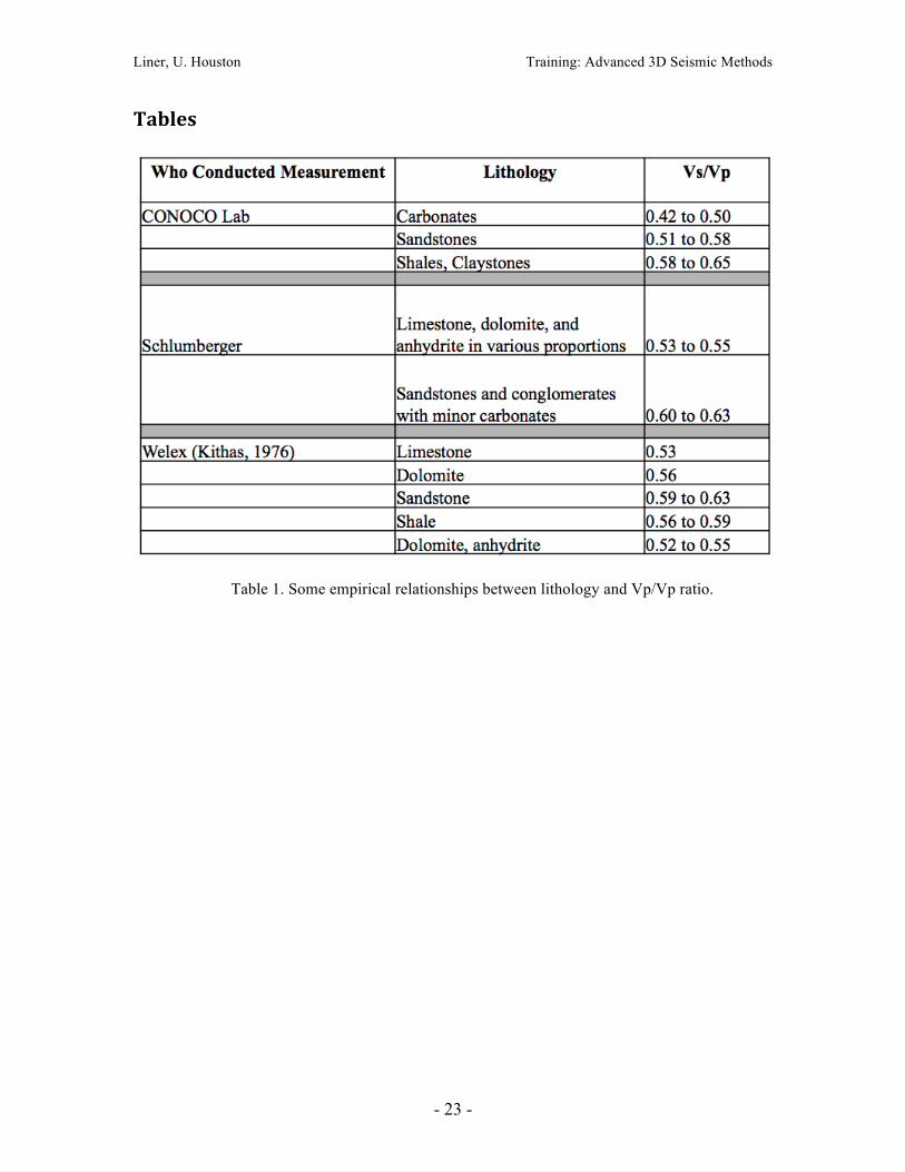
The division of vertical cells of each lithozone was also modified to better reflect the strata occurrence, being equal-height for lithozones within conformable sections (about 20-25 ft) and being truncated as lithozones that encounter the unconformity or lith-boundaries where the cell height reduced to zero. This allows the propagation of properties within the laterally continuous lithozones in the section outside the depth window of the Miss. unconformity, and propagation is stopped where the strata encounter the unconformity or litho boundaries. Figure 5 shows an example of the improved structure model and the resulting porosity grids. The preferred orientation of property propagation is applied only to the sections below the Miss. unconformity, along the direction of open fractures associated with the Pre-Penn structural deformation. The resulting property grid was sliced along the lithozone surfaces to make property maps (Figure 6, example maps). The maps were smoothed (up-scaled) by five rounds of iteration to depict the important trends only. These porosity maps will be compared with the property maps from geophysical and flow modeling. Contour maps of porosity and permeability dumped from the property grid for Lower Cherokee Sandstone reservoir are given in figure 7. Lithology and Vp/Vs ratio assignment from logs (Zeng) Since the project data does not include a full-wave sonic, we will have to estimate S-wave speed from the P-wave sonic and published Vp/Vs ratios. This is summarize in the flow chart of Figure 8. Lithology and fluid volume will affect the S-wave velocity therefore the Vp/Vs ratio, and there are many mixed layers as well as pure shale, sandstone, limestone and dolomite in the Dickman section. Therefore, we have to use lithology discriminators based on 2 or more logs to determine lithology before S-wave speed can be estimated. Four logs can be used in a part of the Sidebottom 6 for this purpose. Based on Jonny’s data sheet (Table 1) and the log data we have in Sidebottom 6, the following two possible work flows were considered to estimate lithology from multiple logs. Both can be started on sections with more than one log (2-4), and extrapolated to the depth interval where not all logs are available, but each has advantages and disadvantages in terms of results and workload.

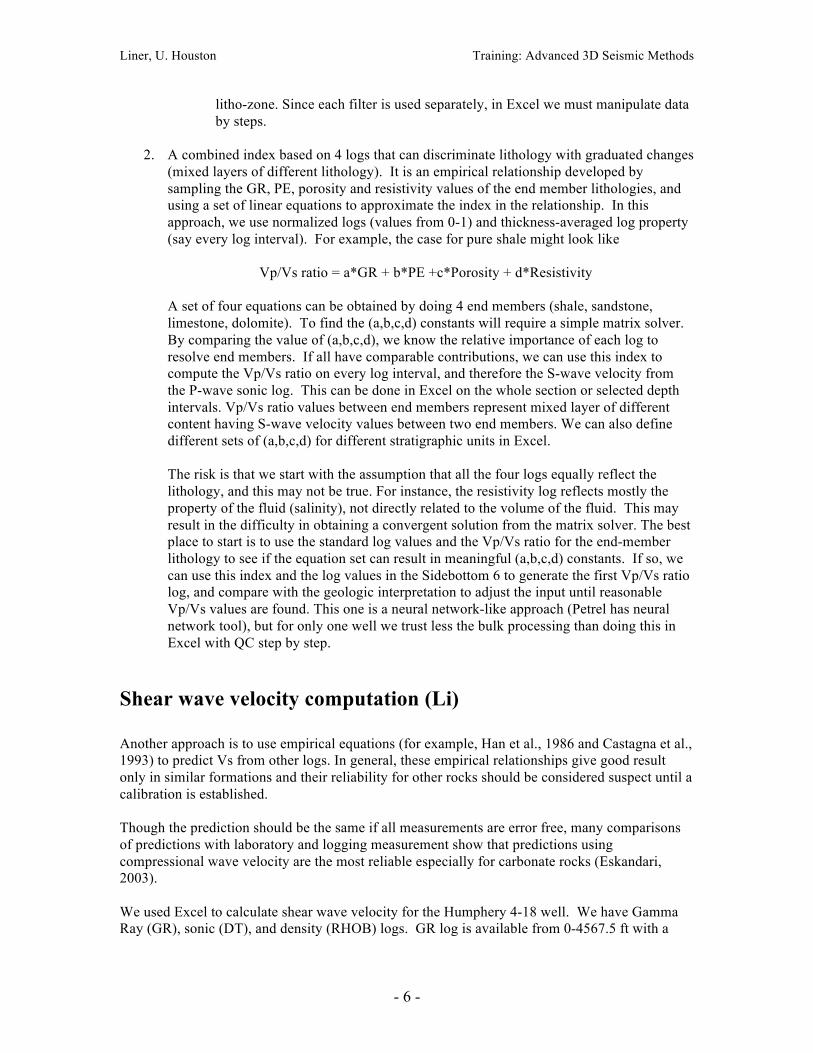
1. A simple index based on 3 logs to break the section into 4 or 5 discrete lithologies. For example, we can use GR, and PE and Porosity (the log name is (NPOR+DPOR)/2 in Sidebottom6) as three filters one by one. The steps are:

a. Gamma Ray (GR) can be used identify shale, sandstone, and carbonate based on cut-off values.

b. Carbonates will be further filtered by PE as limestone or dolomite. The Photo Electronic (PE) log reads the size (area) of the reflecting surfaces of minerals. Pure calcite is the largest, reading around 5. Pure colomite are smaller, 3.14, and pure sandstone is 1.9. We have a limestone-dolomite mixtures and rarely see 5 (mostly between 3.3 and 4.4).

c. The resulting four lithologies are filtered by the porosity (using an imperical criterion, say >5%> 20%) to obtain different zone intervals.

d. For each zone interval, say “porous sandstone”, “tight limestone”, we can assign a P-S ratio based on table 1. The largest number of litho-zones generated by this approach is 4 x 3 = 12, and the thickness index varies with thickness of each


- 6 -

litho-zone. Since each filter is used separately, in Excel we must manipulate data by steps.

2. A combined index based on 4 logs that can discriminate lithology with graduated changes

(mixed layers of different lithology). It is an empirical relationship developed by sampling the GR, PE, porosity and resistivity values of the end member lithologies, and using a set of linear equations to approximate the index in the relationship. In this approach, we use normalized logs (values from 0-1) and thickness-averaged log property (say every log interval). For example, the case for pure shale might look like Vp/Vs ratio = a*GR + b*PE +c*Porosity + d*Resistivity A set of four equations can be obtained by doing 4 end members (shale, sandstone, limestone, dolomite). To find the (a,b,c,d) constants will require a simple matrix solver. By comparing the value of (a,b,c,d), we know the relative importance of each log to resolve end members. If all have comparable contributions, we can use this index to compute the Vp/Vs ratio on every log interval, and therefore the S-wave velocity from the P-wave sonic log. This can be done in Excel on the whole section or selected depth intervals. Vp/Vs ratio values between end members represent mixed layer of different content having S-wave velocity values between two end members. We can also define different sets of (a,b,c,d) for different stratigraphic units in Excel. The risk is that we start with the assumption that all the four logs equally reflect the lithology, and this may not be true. For instance, the resistivity log reflects mostly the property of the fluid (salinity), not directly related to the volume of the fluid. This may result in the difficulty in obtaining a convergent solution from the matrix solver. The best place to start is to use the standard log values and the Vp/Vs ratio for the end-member lithology to see if the equation set can result in meaningful (a,b,c,d) constants. If so, we can use this index and the log values in the Sidebottom 6 to generate the first Vp/Vs ratio log, and compare with the geologic interpretation to adjust the input until reasonable Vp/Vs values are found. This one is a neural network-like approach (Petrel has neural network tool), but for only one well we trust less the bulk processing than doing this in Excel with QC step by step.

Shear wave velocity computation (Li) Another approach is to use empirical equations (for example, Han et al., 1986 and Castagna et al., 1993) to predict Vs from other logs. In general, these empirical relationships give good result only in similar formations and their reliability for other rocks should be considered suspect until a calibration is established. Though the prediction should be the same if all measurements are error free, many comparisons of predictions with laboratory and logging measurement show that predictions using compressional wave velocity are the most reliable especially for carbonate rocks (Eskandari, 2003). We used Excel to calculate shear wave velocity for the Humphery 4-18 well. We have Gamma Ray (GR), sonic (DT), and density (RHOB) logs. GR log is available from 0-4567.5 ft with a


- 7 -

sample interval of 0.5 ft (shown in figure 9), DT is available from 186- 4594 ft, and RHOB from 0- 4597 ft. Based on empirical rules, GR was locally classified into three lithologies, as shown in table below. For each lithology there is a Vp/Vs ratio taken from published studies. Sonic log values are converted into P-wave velocity and the S-wave velocity is computed the appropriate Vp/Vs, resulting in the data shown in Figure 10.

3D Seismic Survey Design and Geometry The simulation 3D survey for Dickman II project is based on a Geokinetics 3D3C design. Several tasks involve testing and determination of parameters related to the design and execution of the new simulated seismic survey. In Table 2 we compare the acquisition parameters and survey properties of the original 2001 survey and the Dickman II simulation survey. From a physics point of view, there are important differences and strengthens that suit the Dickman II survey for CO2 monitoring, verification, and accounting use. Dickman II Survey Design There is a vast literature on the additional benefit of three component (3C) land data relative to single component (Shieh and Hermann, 1990; Stewart et al., 2003). As one example, 3C allows analysis shear wave splitting (Simmons, 2009) while single component data does not. Multi-component or three-component (3C) seismic methods record the full vibration induced in the earth by a seismic survey, horizontal as well as vertical motion is sensed for use in rock property inversion, and fracture detection (Stewart et al., 2002). In the Dickman project, it is essential to accurately determine the subsurface architecture of the target horizons for CO2 emplacement. 3D P-to-S images can assist with the structural interpretation, especially with respect to faults and elastic effects. Once the structure is established, the characteristics of the strata can be estimated by jointly analyzing the pure P-wave data (PP) and converted-wave (PS) results (Stewart et al., 2007). The proposed simulation survey will use multi-component data generated by the Anivec reflectivity modeling program. One trend in seismic acquisition has been a dramatic increase in the number of recording channels. A channel is the pathway into the recording system taken by a seismic trace from a single receiver location. With a small channel count it is not possible to design a survey that is both high fold and full azimuth, affecting data quality and suitability for CO2 MVA work.


- 8 -

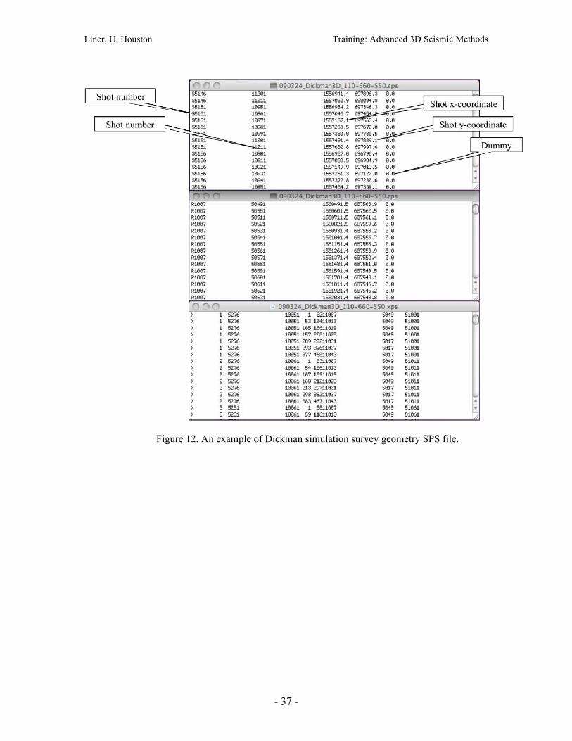
As Table 2 indicates, the small channel count for Dickman I has lead to a common midpoint (CMP) fold of only 25. Higher fold means reduced random noise in the data or, conversely, higher signal-to-noise ratio. The Dickman II simulation survey will have a target CMP fold of 70 (Figure 11a). There have recently been a number of reports demonstrating the dramatic improvement of marine data in complex settings when full azimuth methods are used (verWest and Lin, 2007). For the land CO2 sequestration case, we are not dealing with complex geology, but full azimuth is equally vital as an azimuthal anisotropy indicator (Grechka et al., 2005). The Dickman II simulation survey will be full azimuth (see Figure 11b). When a 3D survey is acquired data is naturally tiled into ‘bins’ and the bin size is determined by shooting parameters. From Table 2 we see that source and receiver intervals in the Dickman I survey are greater than the Dickman II counterparts. The natural bin size of Dickman I is 82.5 x 330 ft, but this has been reduced in processing to a square 82.5 ft bin. The Dickman II simulation survey will have a natural bin size of 55 ft. Traditionally, seismic surveys were acquired with a single active source and interference from other survey sources was considered a form of noise (Silverman, 1979; Lynn et al., 1987; Bagaini, 2006). The Dickman II survey will simulate at least 4 simultaneous sources. Shell Processing Support (SPS) Format The Dickman II simulation survey geometry was generated by Geokinetics in SPS format. The comments below are paraphrased from the SEG standards committee SPS format description. The SPS Format for Land 3D Surveys was originally published by Shell in 1990 and was adopted by the SEG Technical Standards Committee in 1993. This format is established as a common standard for the transfer of positioning and geophysical support data from 3D field crews to seismic processing centers. This standard format contains all relevant field data significantly reduced the time spent by the processing centers on initial quality control and increased the quality of the end products. There are three files in one SPS file with an optional fourth comment file, each with an identical block of header records. The receiver file RPS and source file SPS contain coordinates and elevations of all geophysical points (receiver groups and shotpoints) and of all permanent markers. The cross-reference file XPS show the relation between the receiver groups and shotpoints. The source and cross-reference files are to be sorted chronologically and the receiver file is to be sorted in ascending sequence of line, point and point index numbers. The data set consists of three files with an optional fourth comment file, each with an identical block of header records. For magnetic tapes each file is terminated by a record containing "EOF" in col. 1-3.


- 9 -

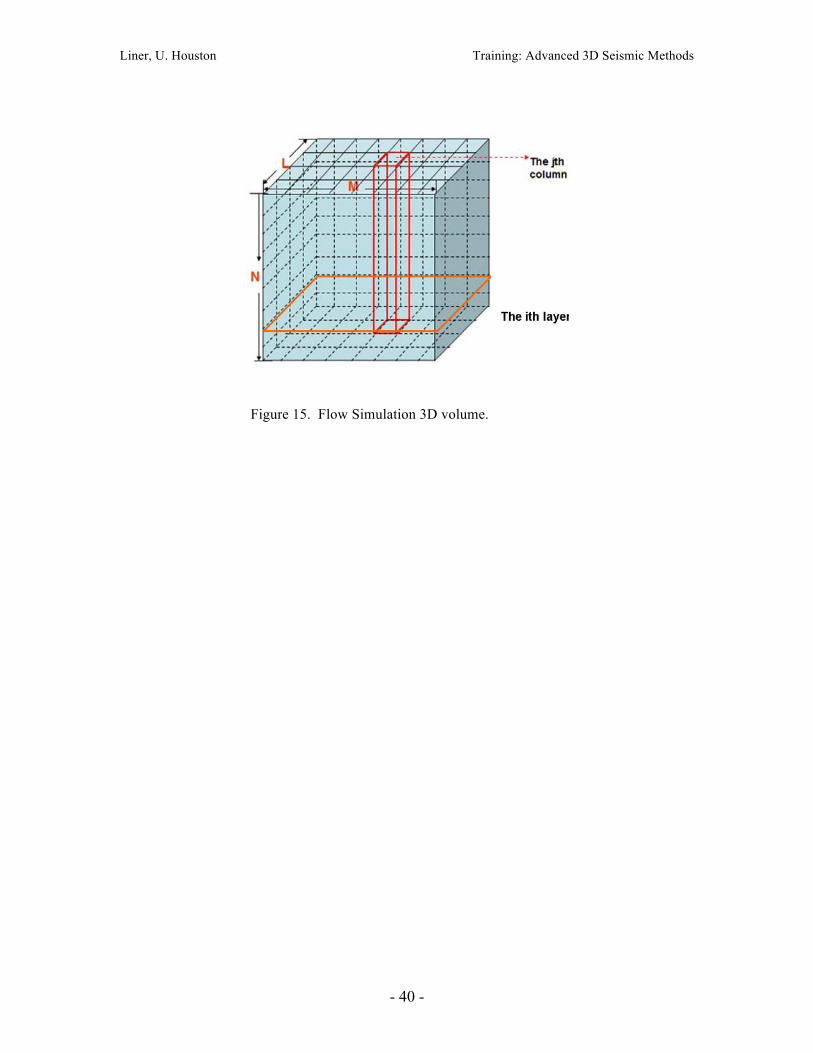
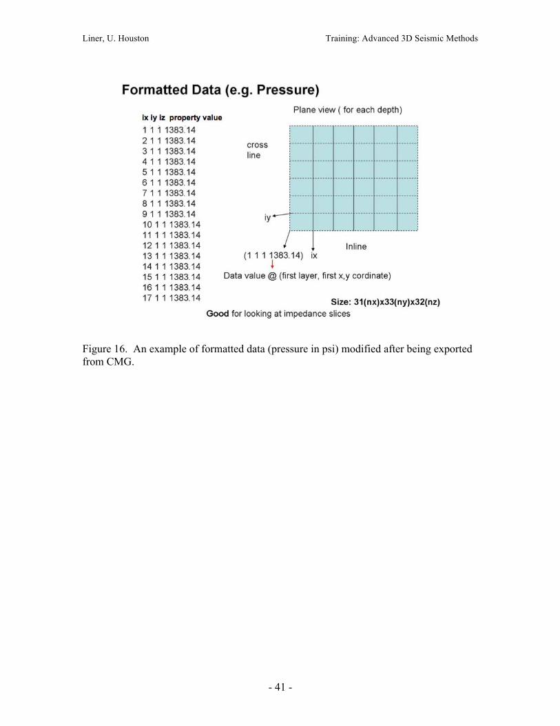
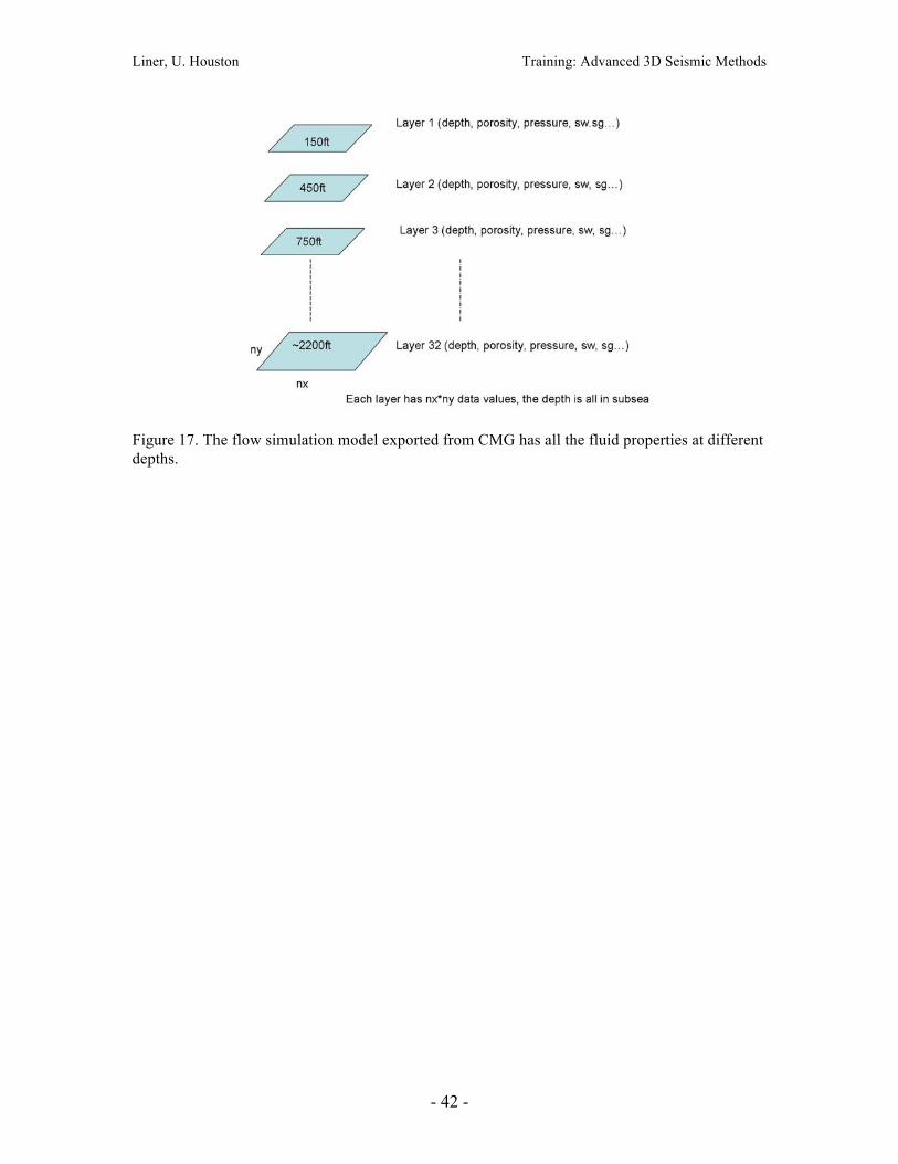
Dickman II Geometry in SPS Format Figure 12 shows an example of Dickman II simulation survey SPS file. The three windows are source (SPS), receiver (RPS) and cross-reference (XPS). And see figure 13 and figure 14 for source and receiver distribution map for Dickman II simulation survey. There are 4233 sources and 3547 receivers in the survey in total. These maps are plotted from the geometry SPS file. For the geometry used in Dicklman II simulation, we use all the receivers live for every shot, so XPS file is not applicable. Seismic response to CO2 injection (Li) This study is to employ time-lapse seismic (4D) to monitor the state of the reservoir, due to changes of fluid properties at periodic times. The change of fluid properties such as fluid saturation, pressure, temperature, porosity etc. will have impact on the seismic responses. Hence, by differencing the seismic responses at varied times the reservoir characteristics can be analyzed. Methods The link between rock physics and seismic modeling is realized by first calculating the seismic velocity and density for the saturated rock at each simulation cell, then calculating seismic reflection coefficients from impedance contrast. Given an input wavelet, seismograms can be generated by some modeling method. A few good candidates can be the modest convolutional model, ray-tracing using Eikonal solver and two-way wave modeling by finite difference. The current CO2 flow simulation calculations utilize the Computer Modeling Group (CMG) generalized equation of state compositional simulator (GEM) which can be used in CO2 enhanced oil recovery and CO2 storage. I used all the requisite parameters from this simulation output into Gassmann's fluid substitution theory. In this case, considering the simulation output as a three-dimensional volume with the size of M x N x L in x, y, z directions, as illustrated in Figure 15. We define the seismic bin size is the same as that of the simulation cell for now, choices of parameters can be changed regarding the seismic resolution. In each bin, we generate the seismic synthetics as a summed trace. For each grid within the seismic bin, we read in all the parameters from the simulation output to calculate impedance, and then calculate the reflection coefficients in this bin. The data format exported from CMG can be accessed at different depths (layers), and each layer contains a set of fluid


- 10 -

properties for fluid substitution calculation (Figure 16 & 17). The reflectivity model can be calculated from different layers first, and then resorted into bins for seismic simulation. The calculations of different bulk modulus of the reservoir are needed as input for the Gassmann equation. They include: bulk modulus for the porous dry rock (Kdry), the solid mineral (Kmin), and the pore fluid (Kfluid). The details are discussed in the following steps. Temperature and Pressure Regime Before calculating the different properties of the saturated rock, the temperature and pressure need to be corrected with depth. Since the bottom-hole temperatures are recorded during logging of the borehole and commonly are not at equilibrium with formation temperature (Carr, Merriam and Bartley, 2005), the temperature (unit: Franheit) for Mississippian is a function of depth:

T=0.0131(depth)+55 (1) For the deep saline acquifer (Arbuckle group)

T=0.0142(depth)+55 (2)

The pressure gradient is 0.476 psi/ft for both the Mississippian and the saline aquifer.

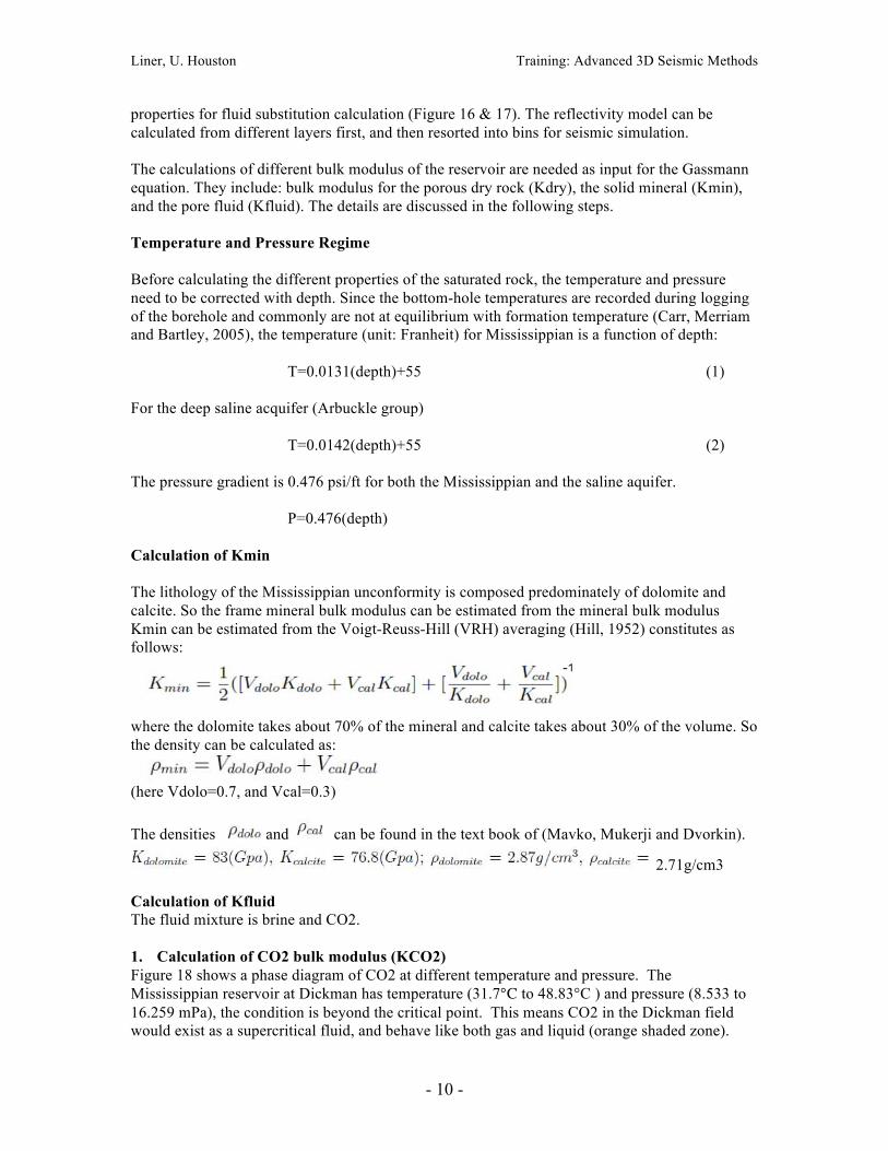
P=0.476(depth) Calculation of Kmin The lithology of the Mississippian unconformity is composed predominately of dolomite and calcite. So the frame mineral bulk modulus can be estimated from the mineral bulk modulus Kmin can be estimated from the Voigt-Reuss-Hill (VRH) averaging (Hill, 1952) constitutes as follows:

where the dolomite takes about 70% of the mineral and calcite takes about 30% of the volume. So the density can be calculated as:

(here Vdolo=0.7, and Vcal=0.3) The densities and can be found in the text book of (Mavko, Mukerji and Dvorkin).

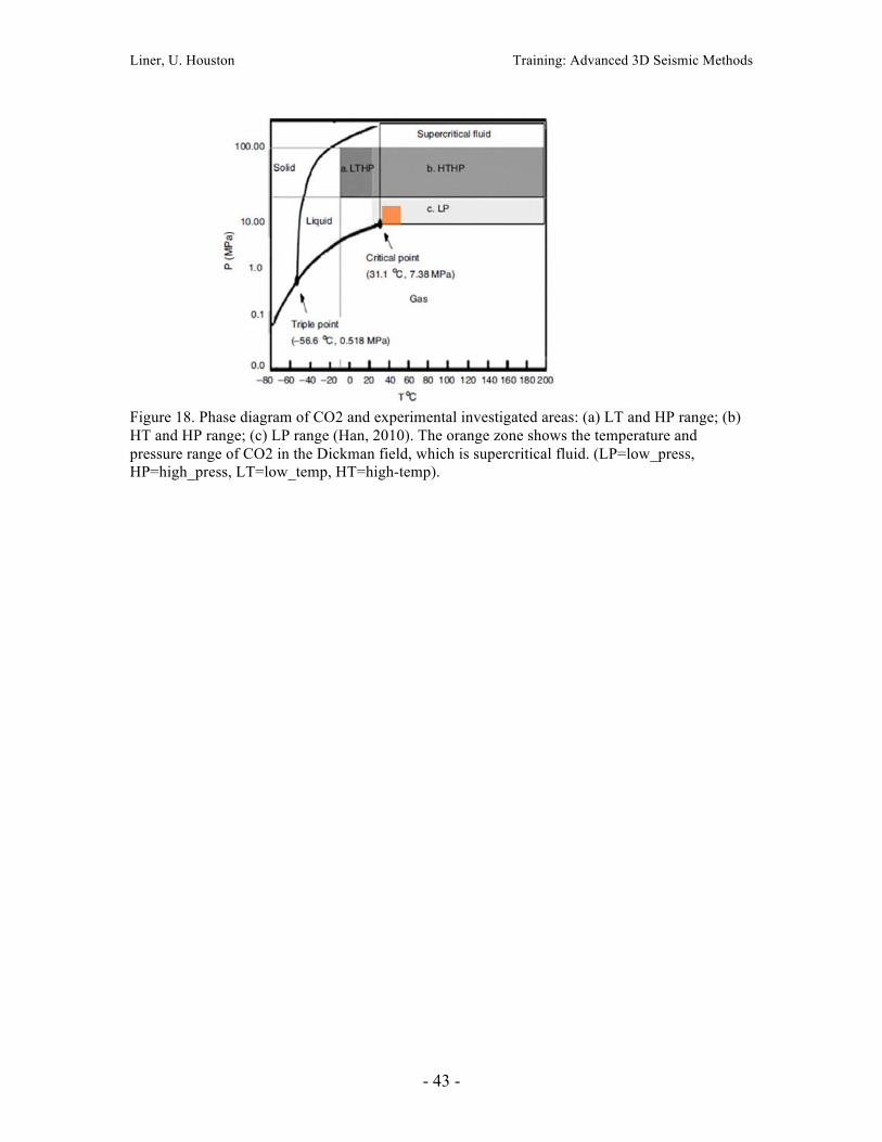
2.71g/cm3 Calculation of Kfluid The fluid mixture is brine and CO2. 1. Calculation of CO2 bulk modulus (KCO2) Figure 18 shows a phase diagram of CO2 at different temperature and pressure. The Mississippian reservoir at Dickman has temperature (31.7°C to 48.83°C ) and pressure (8.533 to 16.259 mPa), the condition is beyond the critical point. This means CO2 in the Dickman field would exist as a supercritical fluid, and behave like both gas and liquid (orange shaded zone).


- 11 -

Han (2010) has done experimental measurements for CO2 velocity at different conditions. They include four T-P regimes:

1) LP: low pressure (7mpa<P<20mpa) ; 2) HP: high pressure ( 20mpa<P<100mpa); 3) HT: high temperature ( 25°C<T<200°C) 4) LT: low temperature (-10°C<T<25°C)

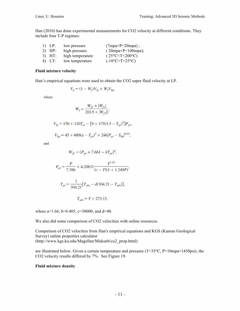
Fluid mixture velocity Han’s empirical equations were used to obtain the CO2 super fluid velocity at LP.

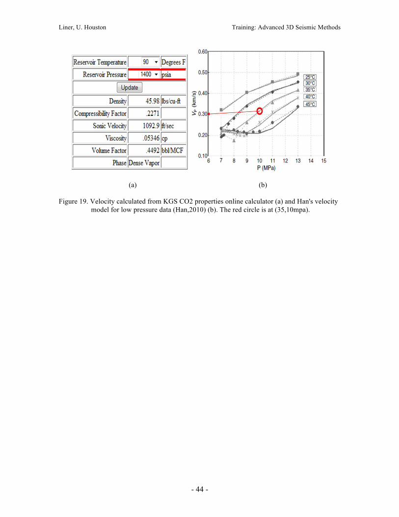
where a=1.66, b=6.405, c=30000, and d=40. We also did some comparison of CO2 velocities with online resources. Comparison of CO2 velocities from Han's empirical equations and KGS (Kansas Geological Survey) online properties calculator (http://www.kgs.ku.edu/Magellan/Midcarb/co2_prop.html) are illustrated below. Given a certain temperature and pressure (T=35°C, P=10mpa=1450psi), the CO2 velocity results differed by 7%. See Figure 19. Fluid mixture density


- 12 -

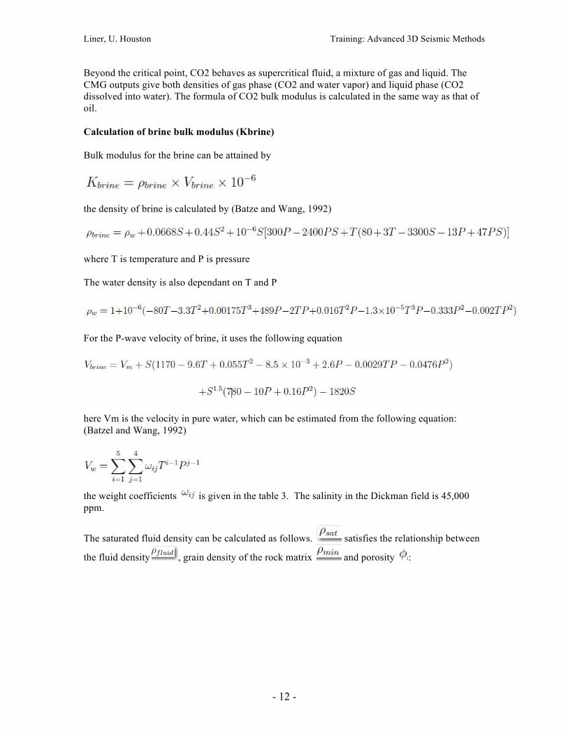
Beyond the critical point, CO2 behaves as supercritical fluid, a mixture of gas and liquid. The CMG outputs give both densities of gas phase (CO2 and water vapor) and liquid phase (CO2 dissolved into water). The formula of CO2 bulk modulus is calculated in the same way as that of oil. Calculation of brine bulk modulus (Kbrine) Bulk modulus for the brine can be attained by

the density of brine is calculated by (Batze and Wang, 1992)

where T is temperature and P is pressure The water density is also dependant on T and P

For the P-wave velocity of brine, it uses the following equation

here Vm is the velocity in pure water, which can be estimated from the following equation: (Batzel and Wang, 1992)

the weight coefficients is given in the table 3. The salinity in the Dickman field is 45,000 ppm.

The saturated fluid density can be calculated as follows. satisfies the relationship between

the fluid density , grain density of the rock matrix and porosity :


- 13 -

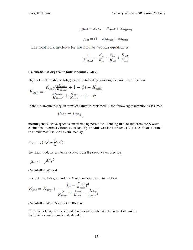
Calculation of dry frame bulk modulus (Kdry) Dry rock bulk modulus (Kdry) can be obtained by rewriting the Gassmann equation

In the Gassmann theory, in terms of saturated rock moduli, the following assumption is assumed

, meaning that S-wave speed is unaffected by pore fluid. Pending final results from the S-wave estimation described earlier, a constant Vp/Vs ratio was for limestone (1.7). The initial saturated rock bulk modulus can be estimated by

the shear modulus can be calculated from the shear wave sonic log

Calculation of Ksat Bring Kmin, Kdry, Kfluid into Gassmann's equation to get Ksat

Calculation of Reflection Coefficient First, the velocity for the saturated rock can be estimated from the following: the initial estimate can be calculated by


- 14 -

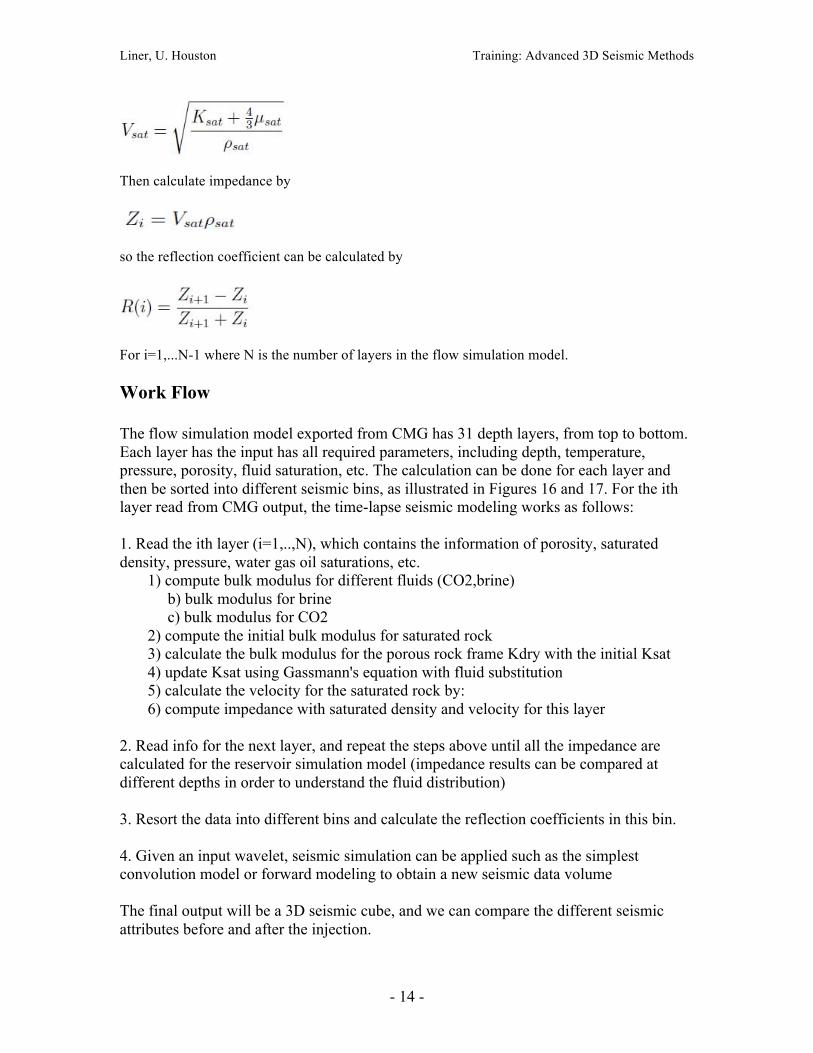
Then calculate impedance by

so the reflection coefficient can be calculated by

For i=1,...N-1 where N is the number of layers in the flow simulation model. Work Flow The flow simulation model exported from CMG has 31 depth layers, from top to bottom. Each layer has the input has all required parameters, including depth, temperature, pressure, porosity, fluid saturation, etc. The calculation can be done for each layer and then be sorted into different seismic bins, as illustrated in Figures 16 and 17. For the ith layer read from CMG output, the time-lapse seismic modeling works as follows: 1. Read the ith layer (i=1,..,N), which contains the information of porosity, saturated density, pressure, water gas oil saturations, etc.

1) compute bulk modulus for different fluids (CO2,brine) b) bulk modulus for brine c) bulk modulus for CO2

2) compute the initial bulk modulus for saturated rock 3) calculate the bulk modulus for the porous rock frame Kdry with the initial Ksat 4) update Ksat using Gassmann's equation with fluid substitution 5) calculate the velocity for the saturated rock by: 6) compute impedance with saturated density and velocity for this layer

2. Read info for the next layer, and repeat the steps above until all the impedance are calculated for the reservoir simulation model (impedance results can be compared at different depths in order to understand the fluid distribution) 3. Resort the data into different bins and calculate the reflection coefficients in this bin. 4. Given an input wavelet, seismic simulation can be applied such as the simplest convolution model or forward modeling to obtain a new seismic data volume The final output will be a 3D seismic cube, and we can compare the different seismic attributes before and after the injection.


- 15 -

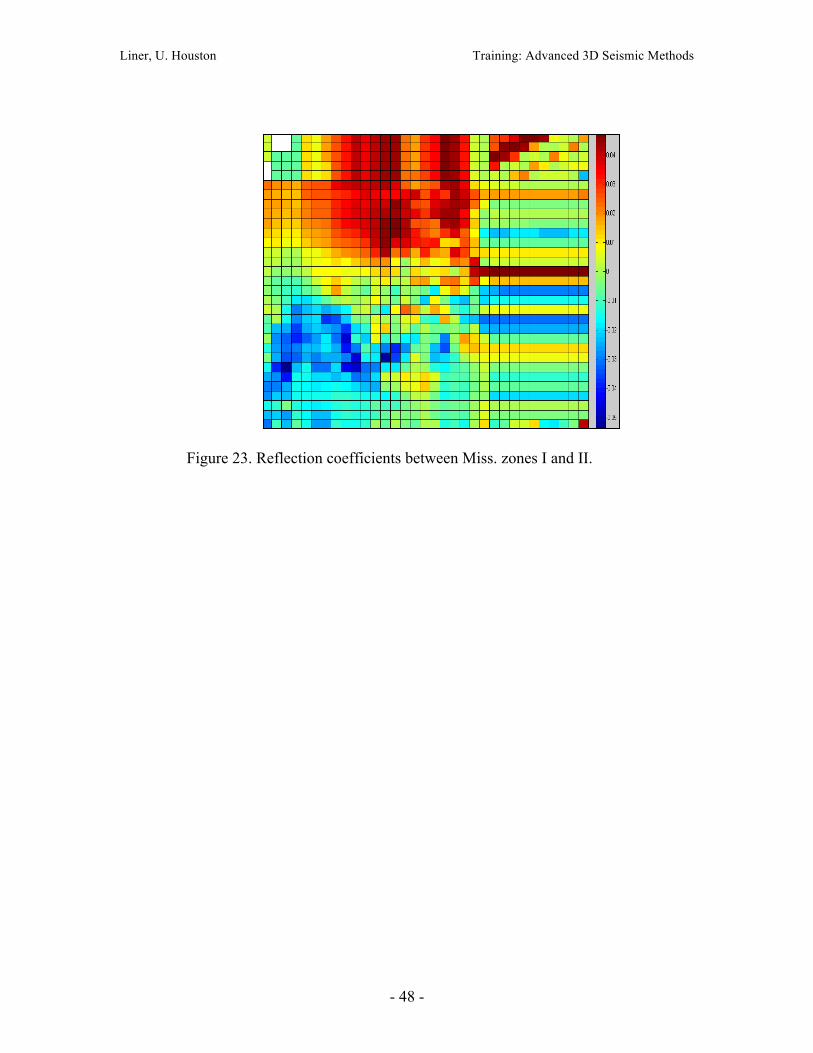
Results The lateral distribution of Mississippian is primarily controlled by depositional facies in carbonate build-ups (Carr et. al., 1999), which is composed of Lower Cherokee sandstone and the rest carbonate is predominantly of limestone. Due to this porous structure, we employed Gassmann therory for calculating the density and velocity for the saturated rock. In the current stage, we computed the reflection coefficients of this depleted oil reservoir at Mississippian-Pennsylvanian unconformity. The depth is around -2000ft subsea. Here we only show one example of reflection coefficients result between Miss porous zone I and II (as illustrated in Figure 18). The scenario is as follows: • Inject CO2 into formation of Porous I and II • Shut in the well for 25 yrs • Mostly brine in porous area and very little CO2, wet zone • Reflection coefficients largely depend on porosity distribution

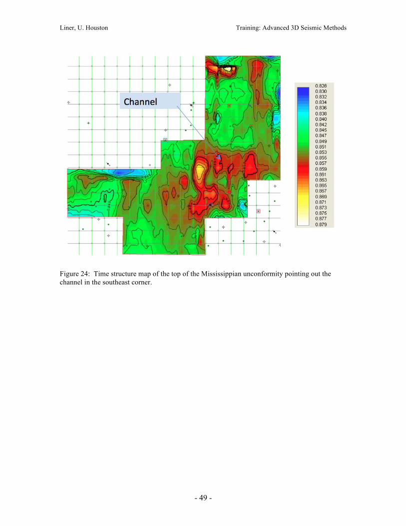
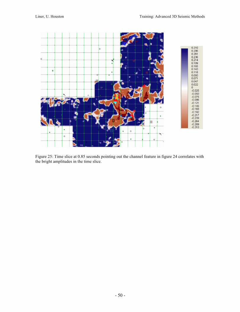
See Figure 19-23 for early results. Mississippian unconformity mapping (Swanson) Analysis of seismic amplitude The amplitude analysis part of this study is to determine if the amplitude at the Mississippian unconformity is the result of porosity, extreme curvature due to Karst, or subtle faulting. The outline of work for this part of the project is to first map the top of the Mississippian unconformity by tying down the seismic response with offset logs and synthetics. Synthetics were created from the Sidebottom 6 well. Although this well is just off of the survey it had a sonic log and drilled deep enough to penetrate the Mississippian formation. The top of the Mississippian was picked along a trough. Preliminary analysis shows the area to have little faulting and mostly a flat structure except for an area in the southeast corner (Figure 24). The time structure map shows this area in the southeast to have areas of depression that appears to be the Mississippian channel feature. A time slice at 0.85 seconds (approximate depth of the Mississippian) shows areas with bright amplitude that correlate with the channel structures on the time structure map (Figure 25). Future work for the next quarter will be to generate geologic modeling parameters to model this channel feature, along with continued research trying to tie geologic parameters to the seismic amplitude a the top of this unconformity. Deep structure mapping (LeBlanc) The storage target being investigated in this section is a porous saline aquifer that lies above the Gilmore city formation (base of the Mississippian) and at the base of the overlying Osage


- 16 -

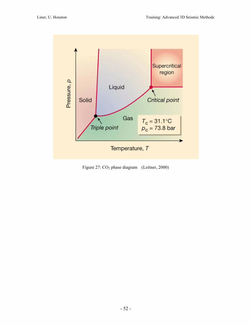
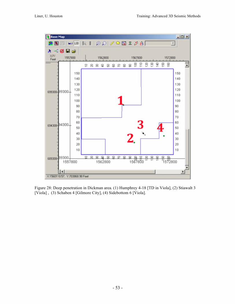
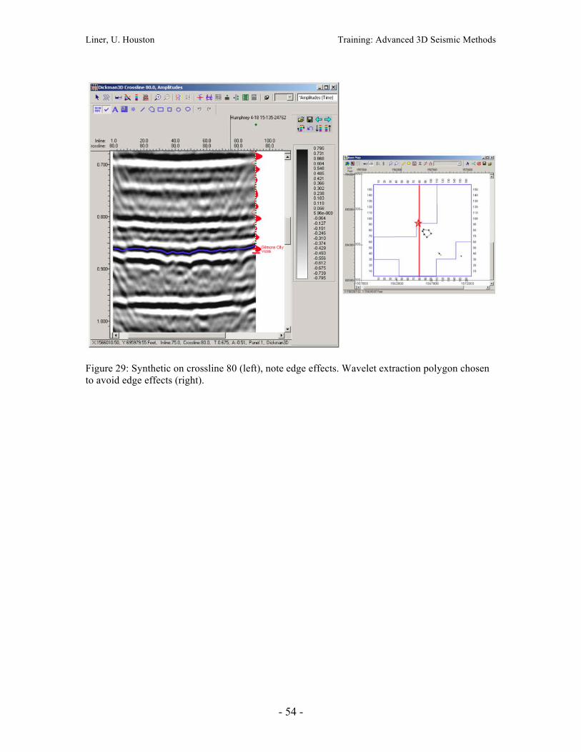
formation. This aquifer is a secondary sequestration target whereas the top of the Mississippian is the primary. See figure 26. Deep saline aquifers have a larger proximity, higher CO2 storage capacity and fewer well penetrations than other proposed storage candidates. In a saline aquifer, CO2 becomes a supercritical fluid beyond 31.1 °C and 7.38 MPa. See figure 27. These are the preferred conditions for this particular storage candidate because the CO2 will have a high density like a fluid but it will be mobile like a gas. The saline aquifer in the Dickman field is part of the Western Interior Plains and Ozark Plateau aquifers that extend for several hundred thousand miles. It has a water flow velocity of about 40 feet per million years meaning that injected CO2 will not migrate to the surface by means of aquifer water flow. Deep saline aquifers are ideal storage candidates because after injection, the CO2 first dissolves, then it ultimately precipitates carbonate minerals. Fang et. al., (2010) states “the reactions among CO2, brine and formation minerals play an important role in formations with a large number of proton sinks, such as feldspar and minerals…some reactions may be beneficial to storage, but others may result in migration pathways.” Therefore, depending on the geological, geochemical and hydrological conditions, these reactions must be thoroughly investigated in order to guarantee safe storage of the carbon dioxide. Investigation of CO2 sequestration involves the use of simulation models and numerous monitoring techniques in order to have a better understanding of how CO2 flows. Data Description/Methodology There are 142 wells in the Dickman Field but only four wells that penetrate the deep horizons of this study. See figure 28 for the locations. Humprey 4-18, Stiawalt 3 and Sidebottom 6 are the only three wells in the Dickman project area that have picks for the Viola and the Gilmore City formations. The Schaben 4 well only penetrates the Gilmore City formation. Investigation of the deep saline aquifer will be primarily seismic since there is minimal well control. The purpose of this investigation is to determine if, by using attributes to map fractures, this deep saline aquifer can be an adequate storage candidate for CO2. It would be preferred to map the Osage formation in addition to the Gilmore City and Viola formations but there is not a velocity or density contrast at the top Osage sufficient to generate a reflection. To begin this study, the geology must first be tied to the 3-D seismic volume (Dickman dataset) by creating synthetic traces using the two wells that have sonic and density logs (Humphrey 4-18 and Sidebottom 6). This will confirm the location of the Gilmore City (base of saline aquifer) and Viola formations in the seismic, which will then allow horizon picking throughout the volume to begin. This process is currently in progress and a preliminary synthetic has been made for each well. To generate the two synthetic wavelets, traces were extracted using a polygon in order to leave out edge effects. See Figure 29. The Humphrey 4-18 will be a much more reliable tie to the geology than the Sidebottom 6. The reason for this is that the Sidebottom 6 is located well outside of the survey area therefore preventing an extraction of traces for comparison. Although, it might be possible to change the x-y coordinates of the Sidebottom 6 well so that it sits inside of the survey. The Humphrey 4-18 synthetic was able to extract traces (extraction area – splice along borehole, trace selection - interpolate) for comparison and a reasonable match has been observed.


- 17 -

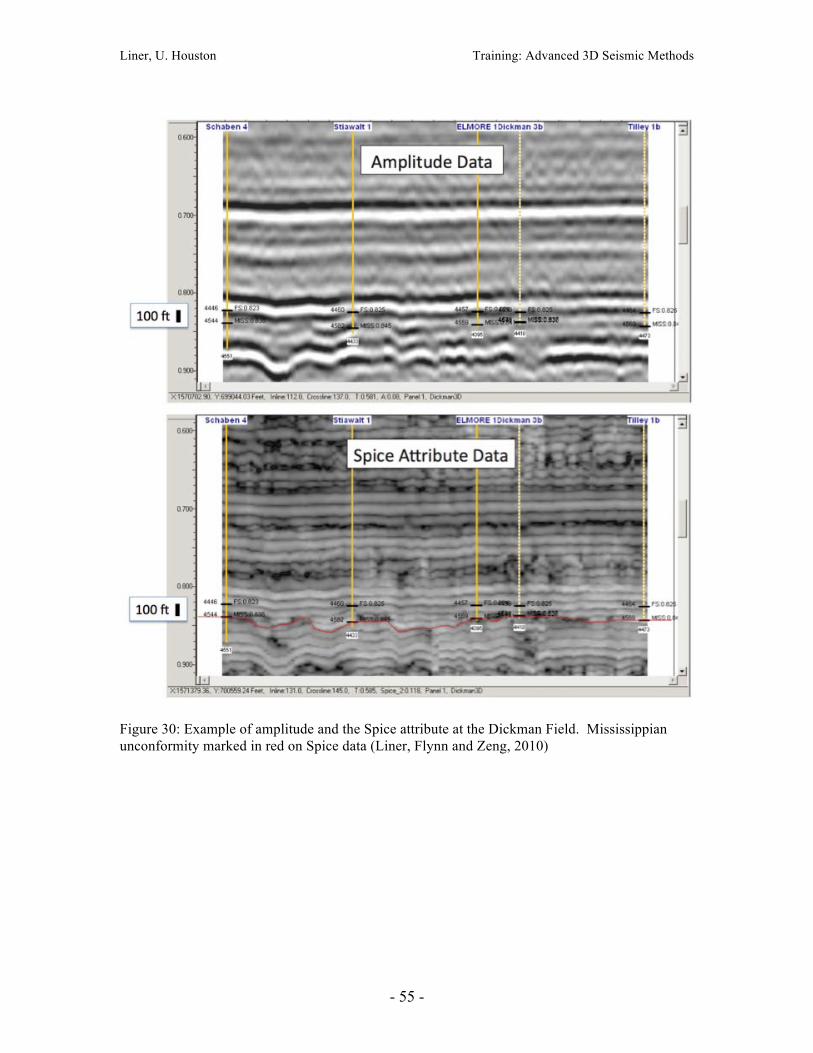
A small phase shift was applied and it had a poor correlation coefficient (0.054) but this is of minimal concern because the main objective for the purposes of this study is to get a good visual match in the deep structure. The Humphrey synthetic places the Gilmore City at a peak and the Viola at a trough. The next step is producing the Gilmore City and Viola time structure maps by tracking these horizons throughout the data. Then, several different attributes will be used for surface mapping. The attributes used in this study focus on identifying the locations of faults and fractures. One attribute that draws attention to these discontinuities is coherence. This attribute uses a cross correlation method to calculate a coherence coefficient from seismic amplitudes on neighboring traces. In other words, it highlights the lateral changes in the waveform. Curvature is another attribute that highlights discontinuities is curvature. This attribute uses reflector dip and azimuth to measure curvature. Curvature more or less, estimates the shape of a reflector. The mathematical definition of curvature is “the inverse of a circle’s radius which is tangent to that surface at that point” (Blumentritt et. al., 2006). Usually the most positive (anticline) and the most negative (syncline) curvature is observed for seismic interpretation. Curvature, for the most part, identifies fractures and faults better than coherence. SPICE (spectral imaging of correlative events) is another general attribute that will help identify fractures. This is somewhat of a new attribute that’s foundation built on wavelet transform decomposition and singularity analysis of migrated seismic data. “The physical basis of SPICE relates to spectral shaping during wave propagation and reflection” (Liner et. al., 2004). Sometimes, residual diffractions can make it difficult to determine a fault from a fold. The spice data gives a much sharper image of this discontinuity and better displays fault localization. Figure 30 shows an example Spice section (not from Dickman data). This study will also use Ant Tracking, an automatic fault extraction technique developed by Petrel. Minimal noise in the volume is preferred and preliminary enhancement of spatial discontinuities using any edge detection algorithm is a required step. The next step is to generate the Ant Track Cube. This Ant Tracking algorithm mimics the ants we know of in nature and their ability of tracking pheromones to find the shortest path between their colony and their food. It gives us a picture of the seismic volume’s so called plumbing system by sending these electronic “ants” into the data so they can detect the fault/fracture surfaces from the edge detection methods (analogous to “pheromones”) previously used (i.e. SPICE, curvature, coherence, etc.). Additional attribute will be applied to the data if time permits.

Summary of significant Events The primary purpose of this research is to simulate a 3D 3C seismic survey over the Dickman area. Key to that effort is receiving the survey design geometry from Geokinetics. This was accomplished this quarter and analysis of the geometry is currently underway.


- 18 -

Work Plan for the Next Quarter For the next quarter, a case study paper will be written by June, and she will give a presentation on the CAPA technology conference on Nov. 3, 2010. Seismic simulation for generating new seismic data with new fluid properties will begin in next quarter. On the same time, we will work on synthetics and further interpretation on Viola, interpret time and depth structure maps towards this formation, run multiple attributes, and eventually estimate storage capacity and depth conversion. Future work on amplitude inversion for the next quarter will be to generate geologic modeling parameters to model the channel feature in the survey, along with continued research trying to tie geologic parameters to the seismic amplitude at the top of this unconformity. Cost and Milestone Status Baseline Costs Compared to Actual Incurred Costs…. Needs update by CLL

7/1/10 – 9/30/10 Plan Costs Difference

Federal $36,668 $49,559 ($12,892) Non-Federal $4,063 $0 $4,063

Total $40,730 $45,559 ($8,829) Forecasted cash needs Vs. actual incurred costs

Notes: (1) Federal plan amount based on award of $293,342 averaged over 8 reporting quarters. (2) Non-Federal plan amount based on cost share of $32,500 averaged as above. (3) Cost this period reflects salary for J. Zeng (3 mo), Q. Wu (3 mo), J. Seales (3 mo), and C. Liner (1 mo).


- 19 -

Continuing Personnel Prof. Christopher Liner is Principle Investigator and lead geophysicist. He is a member of the SEG CO2 Committee, Associate Director of the Allied Geophysical Lab, and has been selected to deliver the 2012 SEG Distinguished Instructor Short Course. Dr. Jianjun (June) Zeng has been working exclusively on this project since Dec 2007 and is lead geologist. Ms. Qiong Wu is a graduate PHD student in geophysics who joined the project in January 2010 as a research assistant. She will be funded year-round out of the project. Mr. Johnny Seales is an undergraduate student majoring in Geology and Geophysics. He is also a U.S. Army veteran, having served in Iraq. He will be funded year-round from the project. He anticipates earning his undergraduate degree in Dec. 2011. Ms. Jintan Li is a PhD student in geophysics who joined the project in Aug 2009. She is funded by Allied Geophysical lab at this time. Her thesis will be time-lapse seismic modeling (4D) for conducting dynamic reservoir characterization of the Dickman Field. Ms. Shannon Leblanc received her bachelor’s in geology at the University of Louisiana at Lafayette and is now pursuing a master’s degree in geophysics at the University of Houston. She is the current SEG student chapter president and joined the CO2 group in January of 2010. Shannon is mapping deep structure in the Dickman Field to determine the potential of a deep saline aquifer as a CO2 storage candidate. Mr. Eric Swanson is a part time graduate MS student in geophysics who joined the project in July 2010 and works full-time for Swift Energy.

Technology Transfer Activities Two presentations are accepted for presentation at the AAPG and SPE Annual Meeting. See Appendix I and II for detail.

Contributors Christopher Liner (P.I, Geophysics) Jianjun (June) Zeng (Geology and Petrel Modeling) Qiong Wu (Geophysics PhD candidate) Johnny Seales (Geology and Geophysics Undergraduate) Jintan Li (Geophysics PhD candidate) Shannon Leblanc (Geophysics MS candidate) Eric Swanson (Geophysics MS candidate)


- 20 -

References Blumentritt, C.H., Marfurt, K.J. and Sullivan, C.E., 2006, Volume-based Curvature Computations Illuminate Fracture Orientations – Early to Mid-Paleozoic, Central Basin Platform, West Texas: Geophysics, Vol. 71, NO. 5, B159-166 Chopra, S. and Marfurt, K., 2008, Seismic Attributes for Stratigraphic Feature Characterization: Back to Exploration-CSPG CSEG CWLS Convention Fang, Y., Baojun, B., Dazhen, T., Dunn-Norman, S. and Wronkiewcz, D., 2010, Characteristics of CO2 Sequestration in saline aquifers: Pet. Sci. 7:83-92 Han, Sun and Batzle: CO2 velocity measurement and models for temperatures up to 200°C and pressures up to 100 MPa, GEOPHYSICS,VOL. 75, NO. 3P. E123–E129 Jewett, J.M., Bayne, C.K., Goebel, E.D., O’Connor, H.G., Swineford, A. and Zeller, D.E., 1968, The Stratigraphic Succession in Kansas: Kansas Geological Survey Bulletin, 189 Liner, C., Li, C.F., Gersztenkorn, A., and Smythe, J., 2004, SPICE: A New General Seismic Attribute: SEG Int’l Exposition and 74th Annual Meeting Liner, C., Zeng, J., Geng, P., King, H., Li, J., Califf, J. and Seales, J., 2010a, 3D Seismic Attributes and CO2 Sequestration: DOE Final Report Liner, C., Flynn, B., and Zeng, 2010, Case History: Spicing up mid-continent seismic interpretation, SEG Expanded Abstracts, 29 , no. 1, 1317-1321. Plasynski, S, D. Deel, L. Miller, and B. Kane, 2007, Carbon sequestration technology roadmap and program plan: U.S. Department of Energy, Office of Fossil Energy, National Energy Technology Laborator, e-report Sawyers, C. and Wilson, T., 2010, An Introduction to this Special Section: CO2 Sequestration: The Leading Edge, 29, 148-149


- 21 -

Appendix I: AAPG Abstract (Submitted) 3D Geologic Modeling toward a Site-specific CO2 Injection Simulation. Jianjun Zeng1, Christopher L. Liner1, Po Geng1, Heather King1, A solid geological model at reservoir scale is the key starting point toward a site-specific characterization of a CO2 sequestration target. In the Dickman Field of Ness County, Kansas, a 3D structure and property model was built for depleted reservoirs of carbonates and clastic rocks through multi-scale data integration. Work flows were designed to handle some of the challenges commonly involved in geological modeling at the reservoir-scale: targeting geological features normally considered as “sub-seismic” and beyond the resolution of conventional seismic stratigraphy; recognizing the lateral heterogeneity in acoustic properties of laterally interwoven clastics and carbonate lithologies on a karst-modified paleo-topography to restore true subsurface geometry; calibrating legacy well logs to obtain reservoir properties with quantified risk assessments; and extracting a fault-fracture framework from multiple seismic attribute volumes to guide the reservoir property gridding. As a first step, a depth-converted stratgraphic model was established and validated by log interpretations at 17 well sites. Fault and fracture analysis was based on seismic interpretation and volumetric attributes, supported by log and core evidences and understanding of the regional deformation history. A unique set of porosity was assigned to the stratigraphic model through calibrating porosity logs of different types and correlating log to core measurements. Permeability estimation was based on core measurements available in Dickman and the surrounding oil fields. Water saturation measured from flushed cores was calibrated to the in-situ water saturation. The propagation of these reservoir properties through the model was along preferred orientations guided by fracture and acoustic impedance analysis. The resulting property grid was tested by production history-matching simulation. A reasonable match was obtained after two rounds of input parameter adjustment and the inclusion of a capillary zone in the model. The initial geological model built from heavily drilled reservoirs was extended to deeper saline aquifers with only three well controls, aided by 3D seismic impedance analysis. The grid served as input to CO2 injection simulations for the deep saline aquifer, a potential carbon capture and sequestration target.


- 22 -

Appendix II: SPE Abstract (Submitted) A CO2 Sequestration Simulation Case Study at the Dickman Field, Ness Co., Kansas Christopher L. Liner, Po Geng, Jianjun Zeng, Heather King and Jintan Li, U. of Houston Since 2006 University of Houston has been funded by DOE to evaluate the Dickman area for suitability as a permanent underground CO2 storage site. This paper is a summary on the simulation part of the project.

Combining 3D seismic and dense well control, a static model was constructed. After the history matching validation, various different deep saline aquifer simulation models were constructed to study the CO2 injection rate and storage safety issues. A full formation simulation model including sallow geological layers and deep saline aquifer was further constructed to predict CO2 migration after injection.

History matching validation has proven to be difficult due to lack of pressure data and early records of water production. An acceptable result was obtained only after many iterations and model modifications. Free CO2 gas trapped in a geological structure can migrate to the surface through faults, fractures, a failed cap rock, or corroded well pipe. These actions represent a real safety threat. A major challenge is to develop a practical simulation model to predict possible CO2 leakage rate and time after injection. A feasible way of improving CO2 storage safety is to accelerate residual gas and solubility trapping. Our simulation results indicate two effective ways of reducing free CO2: injecting CO2 with brine, and/or horizontal well injection. A tuned combination of these methods can reduce the amount of free CO2 in the aquifer from over 50% to less than 10%.

As part of the huge Western Interior Plains aquifer system, the aquifer under the Dickman field may be an ideal CO2 storage site. However, the complicated geological structure and numerous abandoned wells cast uncertainty on its ability to serve as a permanent CO2 storage site. This study will demonstrate that a careful simulation study can maximize CO2 injection rate, minimize existence of free CO2 and significantly reduce the uncertainty in the safety of CO2 permanent storage.


- 23 -

Tables

Table 1. Some empirical relationships between lithology and Vp/Vp ratio.


- 24 -

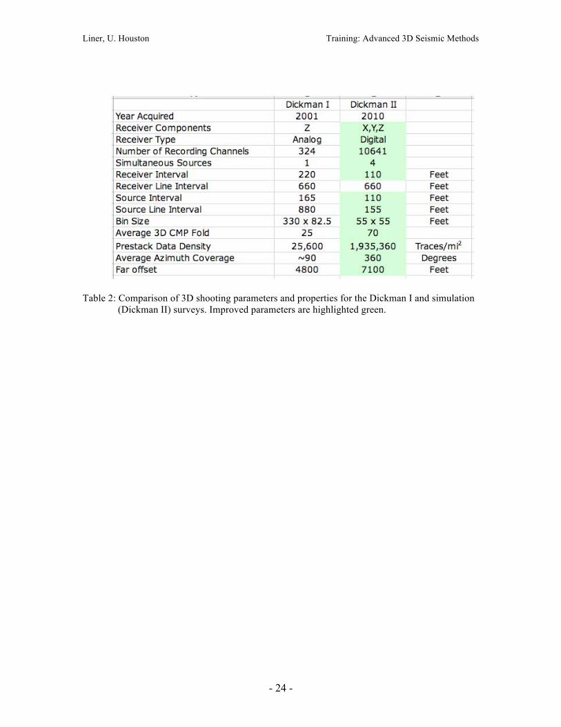
Table 2: Comparison of 3D shooting parameters and properties for the Dickman I and simulation (Dickman II) surveys. Improved parameters are highlighted green.


- 25 -

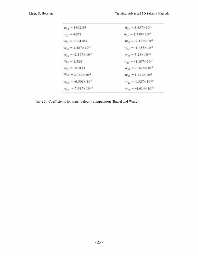
Table 3. Coefficients for water velocity computation (Batzel and Wang).


- 26 -

Figures

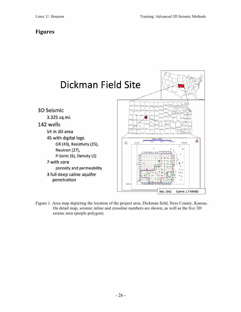
Figure 1. Area map depicting the location of the project area, Dickman field, Ness County, Kansas. On detail map, seismic inline and crossline numbers are shown, as well as the live 3D seismc area (purple polygon).


- 27 -

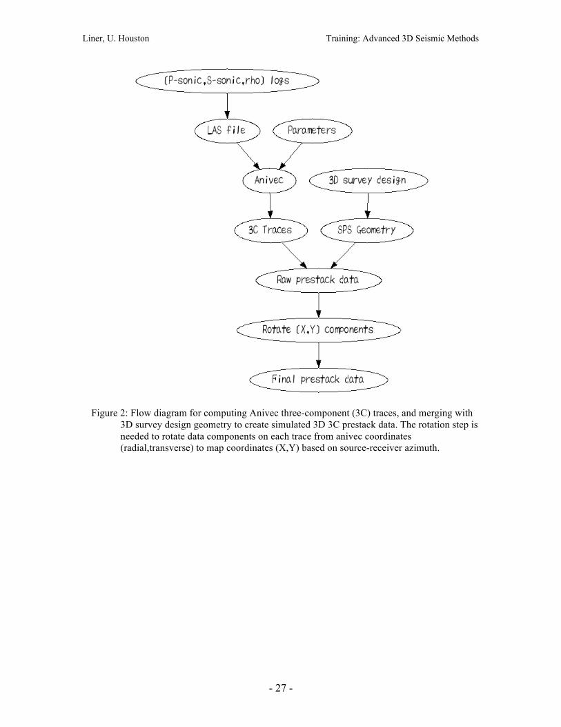
Figure 2: Flow diagram for computing Anivec three-component (3C) traces, and merging with 3D survey design geometry to create simulated 3D 3C prestack data. The rotation step is needed to rotate data components on each trace from anivec coordinates (radial,transverse) to map coordinates (X,Y) based on source-receiver azimuth.


- 28 -

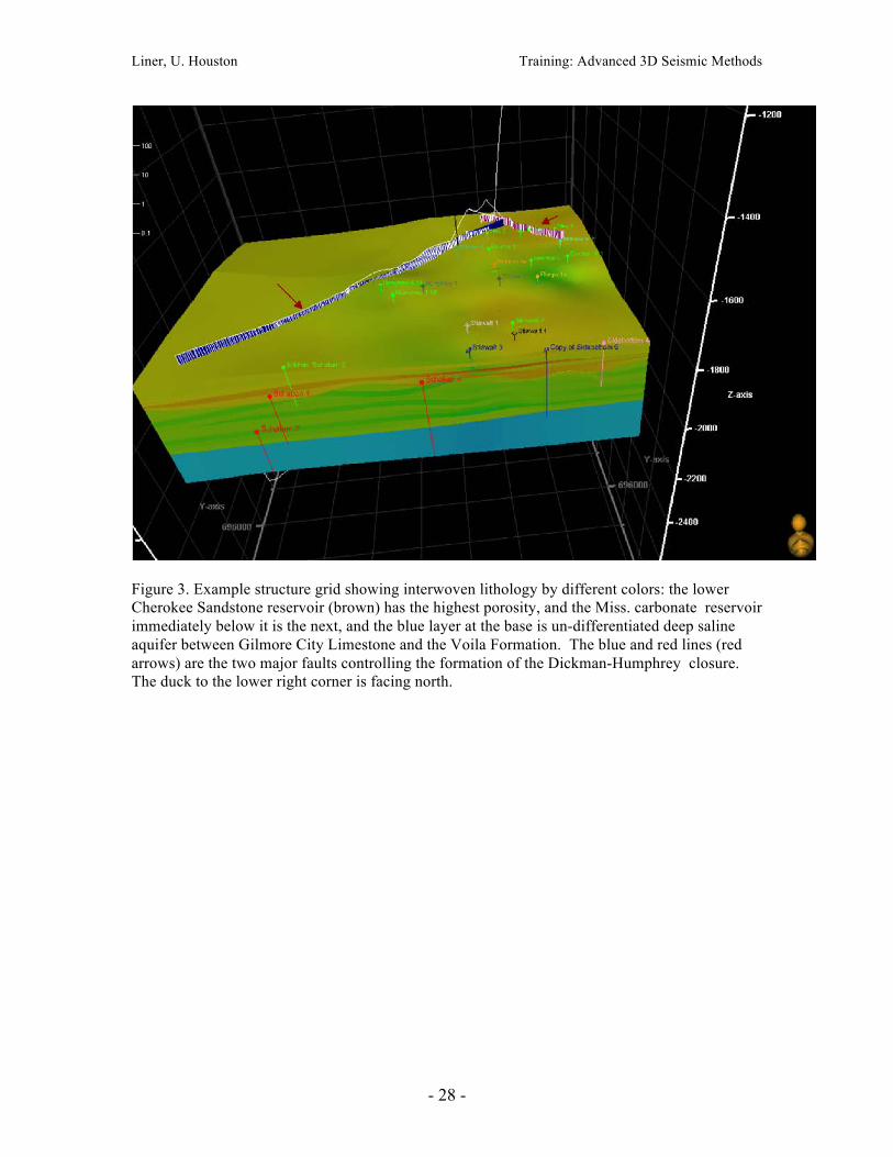
Figure 3. Example structure grid showing interwoven lithology by different colors: the lower Cherokee Sandstone reservoir (brown) has the highest porosity, and the Miss. carbonate reservoir immediately below it is the next, and the blue layer at the base is un-differentiated deep saline aquifer between Gilmore City Limestone and the Voila Formation. The blue and red lines (red arrows) are the two major faults controlling the formation of the Dickman-Humphrey closure. The duck to the lower right corner is facing north.


- 29 -

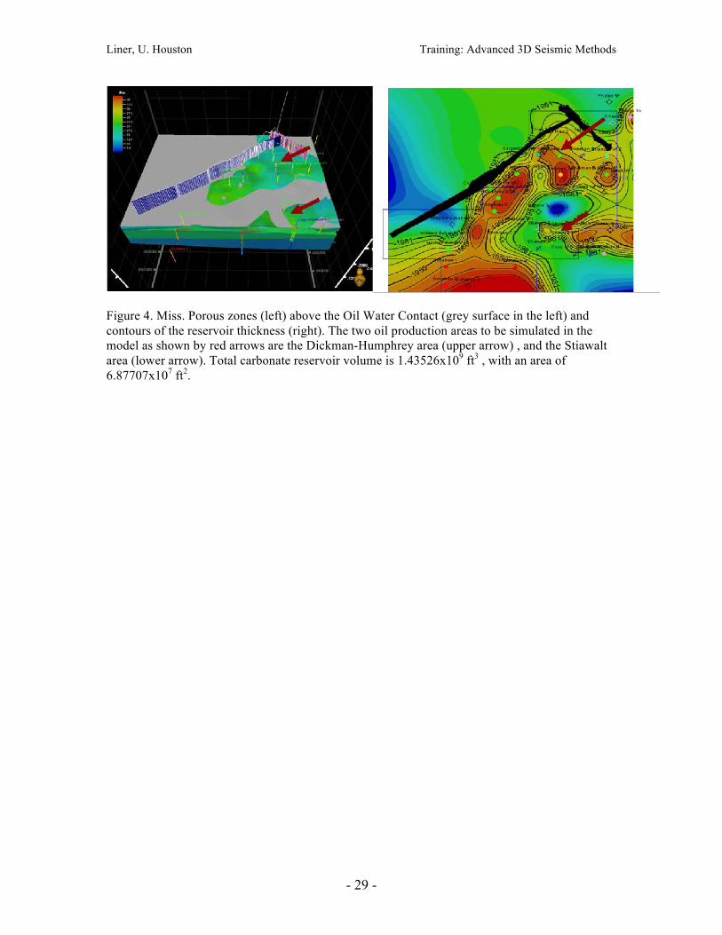
Figure 4. Miss. Porous zones (left) above the Oil Water Contact (grey surface in the left) and contours of the reservoir thickness (right). The two oil production areas to be simulated in the model as shown by red arrows are the Dickman-Humphrey area (upper arrow) , and the Stiawalt area (lower arrow). Total carbonate reservoir volume is 1.43526x109 ft3 , with an area of 6.87707x107 ft2.


- 30 -

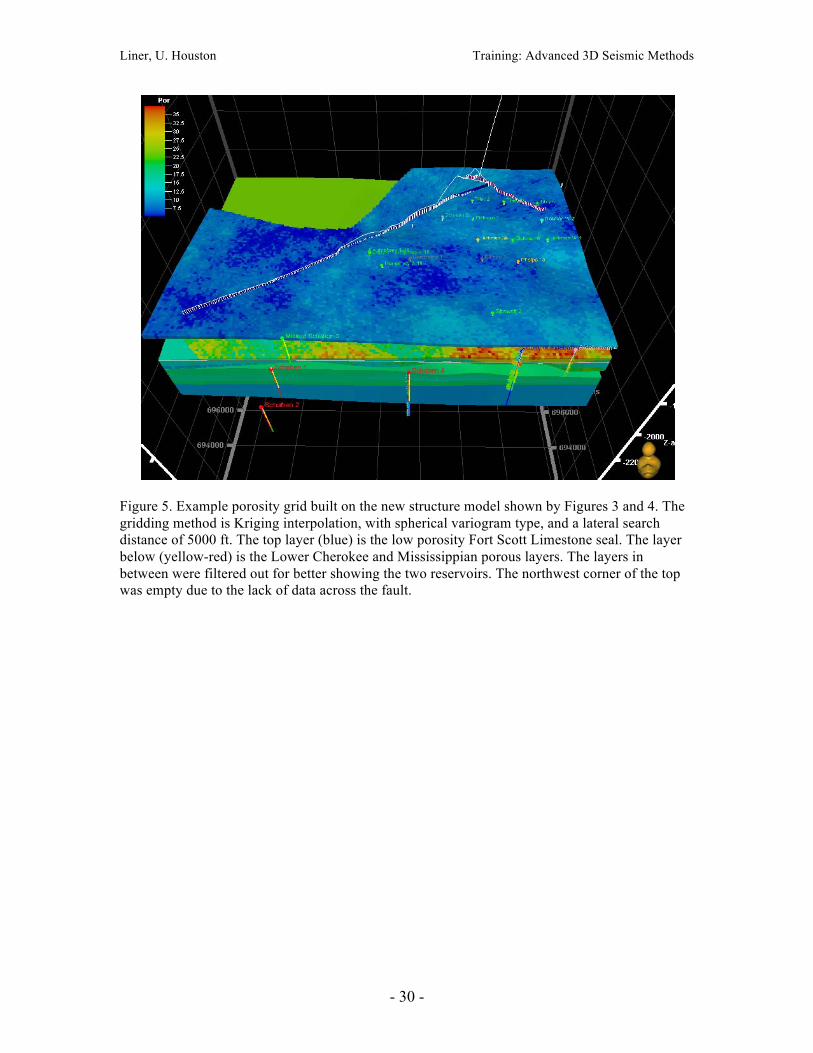
Figure 5. Example porosity grid built on the new structure model shown by Figures 3 and 4. The gridding method is Kriging interpolation, with spherical variogram type, and a lateral search distance of 5000 ft. The top layer (blue) is the low porosity Fort Scott Limestone seal. The layer below (yellow-red) is the Lower Cherokee and Mississippian porous layers. The layers in between were filtered out for better showing the two reservoirs. The northwest corner of the top was empty due to the lack of data across the fault.


- 31 -

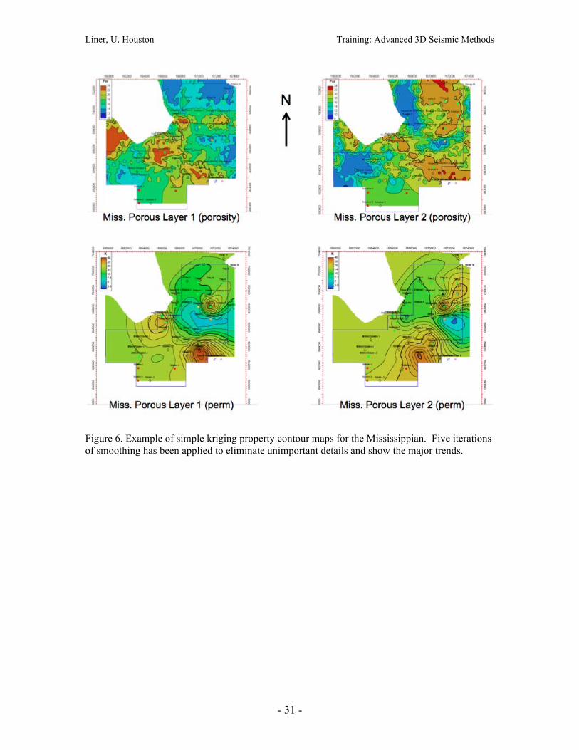
Figure 6. Example of simple kriging property contour maps for the Mississippian. Five iterations of smoothing has been applied to eliminate unimportant details and show the major trends.


- 32 -

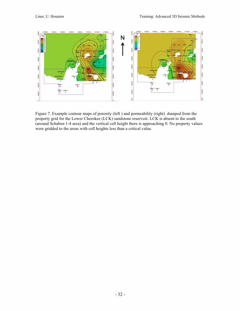
Figure 7. Example contour maps of porosity (left ) and permeability (right) dumped from the property grid for the Lower Cherokee (LCK) sandstone reservoir. LCK is absent to the south (around Schaben 1-4 area) and the vertical cell height there is approaching 0. No property values were gridded to the areas with cell heights less than a critical value.


- 33 -

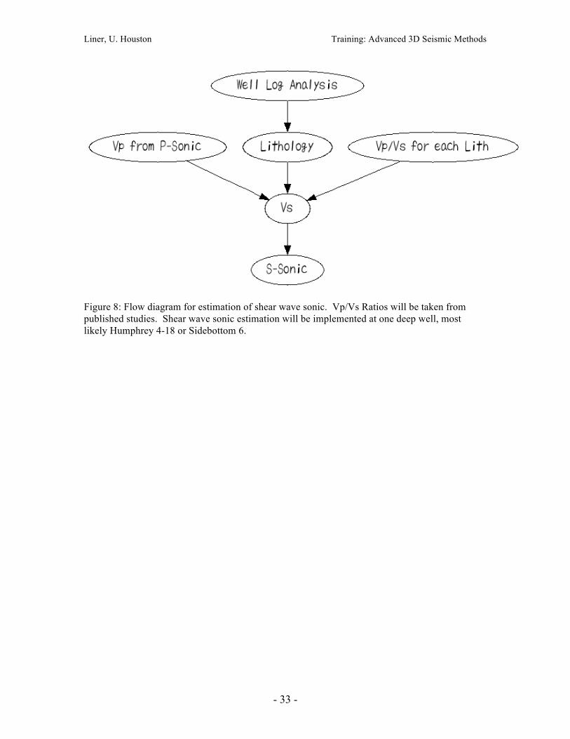
Figure 8: Flow diagram for estimation of shear wave sonic. Vp/Vs Ratios will be taken from published studies. Shear wave sonic estimation will be implemented at one deep well, most likely Humphrey 4-18 or Sidebottom 6.


- 34 -

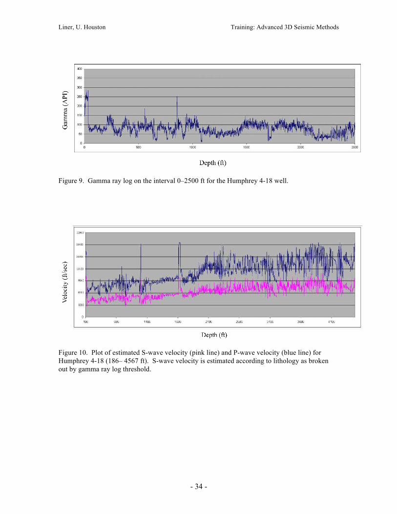
Figure 9. Gamma ray log on the interval 0–2500 ft for the Humphrey 4-18 well.

Figure 10. Plot of estimated S-wave velocity (pink line) and P-wave velocity (blue line) for Humphrey 4-18 (186– 4567 ft). S-wave velocity is estimated according to lithology as broken out by gamma ray log threshold.


- 35 -

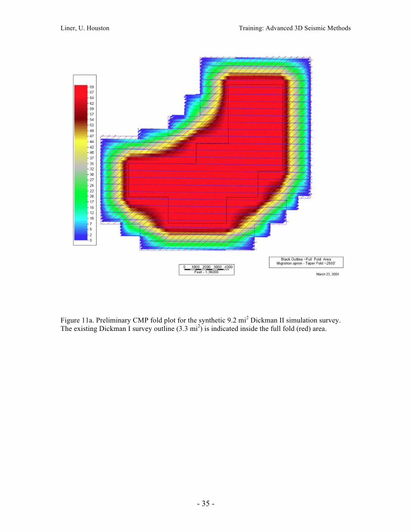
Figure 11a. Preliminary CMP fold plot for the synthetic 9.2 mi2 Dickman II simulation survey. The existing Dickman I survey outline (3.3 mi2) is indicated inside the full fold (red) area.


- 36 -

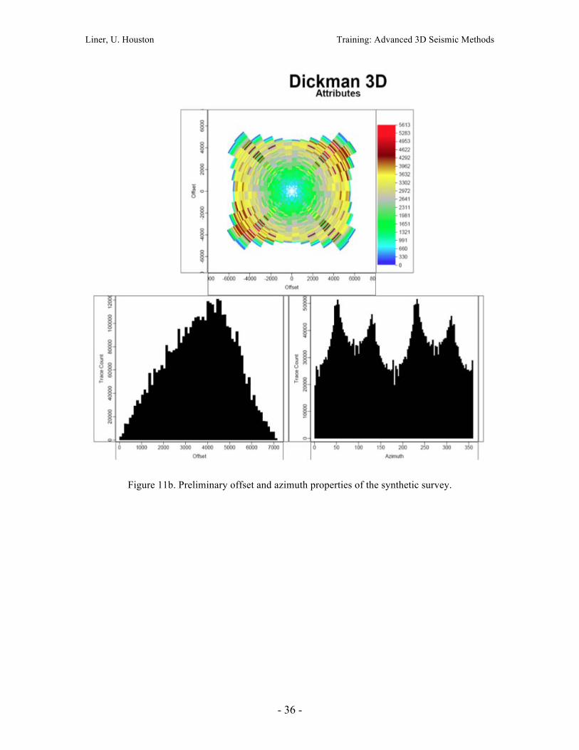
Figure 11b. Preliminary offset and azimuth properties of the synthetic survey.


- 37 -

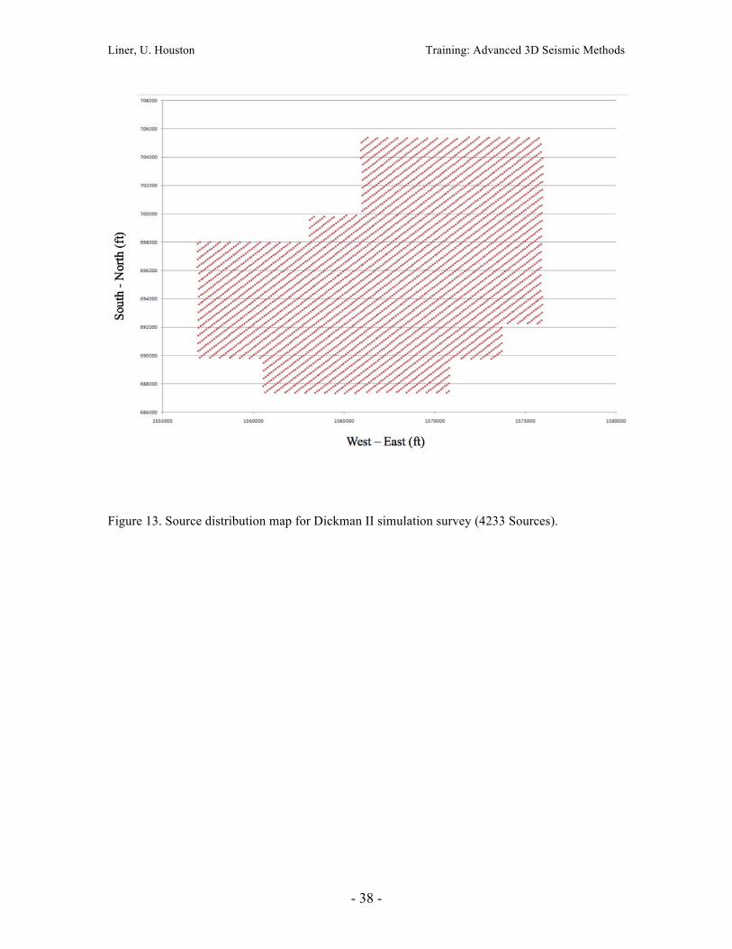
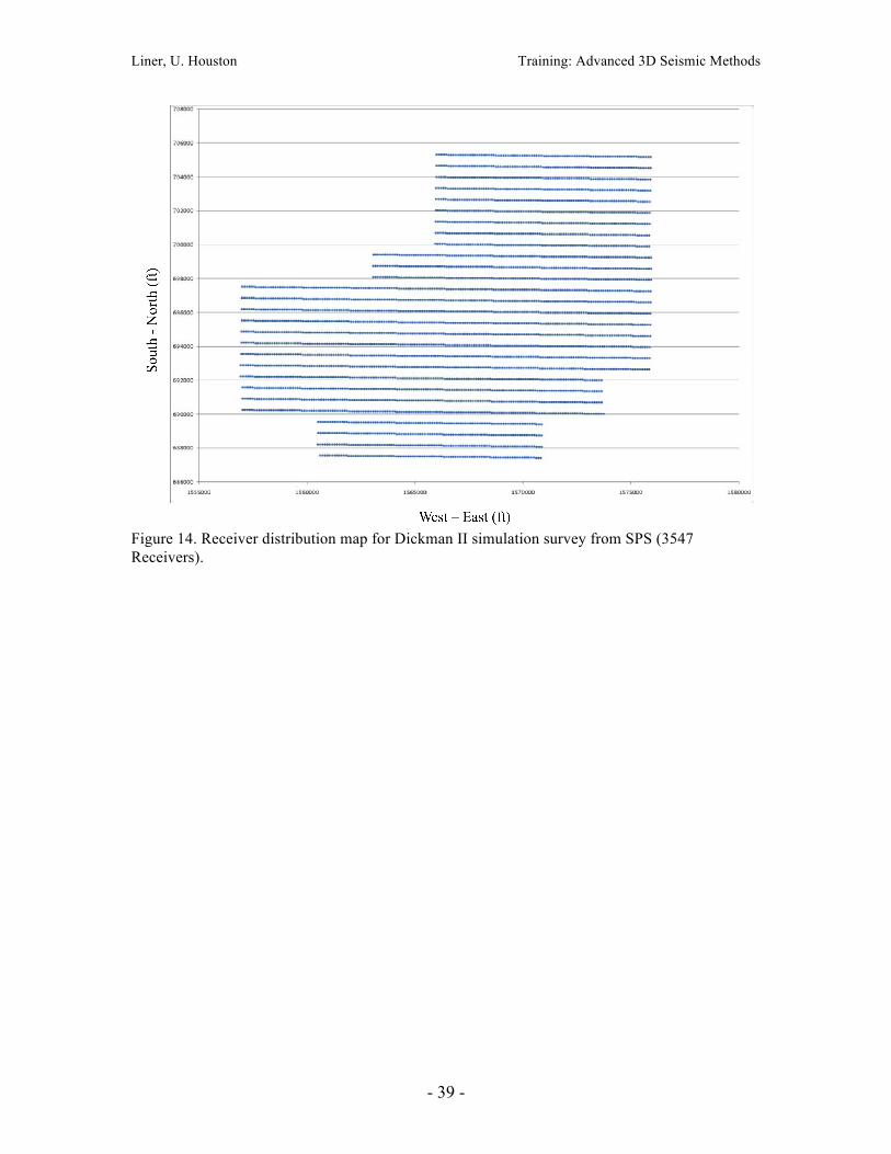
Figure 12. An example of Dickman simulation survey geometry SPS file.


- 38 -

Figure 13. Source distribution map for Dickman II simulation survey (4233 Sources).


- 39 -

Figure 14. Receiver distribution map for Dickman II simulation survey from SPS (3547 Receivers).


- 40 -

Figure 15. Flow Simulation 3D volume.


- 41 -

Figure 16. An example of formatted data (pressure in psi) modified after being exported from CMG.


- 42 -

Figure 17. The flow simulation model exported from CMG has all the fluid properties at different depths.


- 43 -

Figure 18. Phase diagram of CO2 and experimental investigated areas: (a) LT and HP range; (b) HT and HP range; (c) LP range (Han, 2010). The orange zone shows the temperature and pressure range of CO2 in the Dickman field, which is supercritical fluid. (LP=low_press, HP=high_press, LT=low_temp, HT=high-temp).


- 44 -

(a) (b) Figure 19. Velocity calculated from KGS CO2 properties online calculator (a) and Han's velocity model for low pressure data (Han,2010) (b). The red circle is at (35,10mpa).


- 45 -

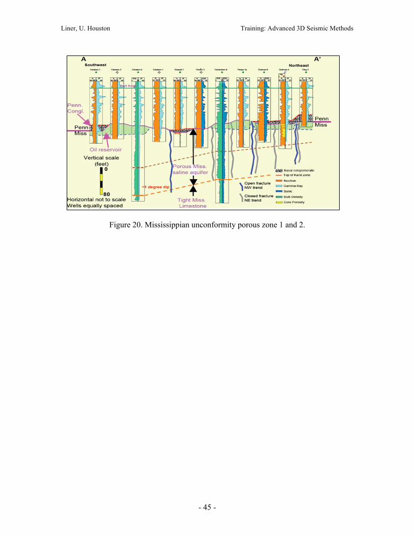
Figure 20. Mississippian unconformity porous zone 1 and 2.


- 46 -

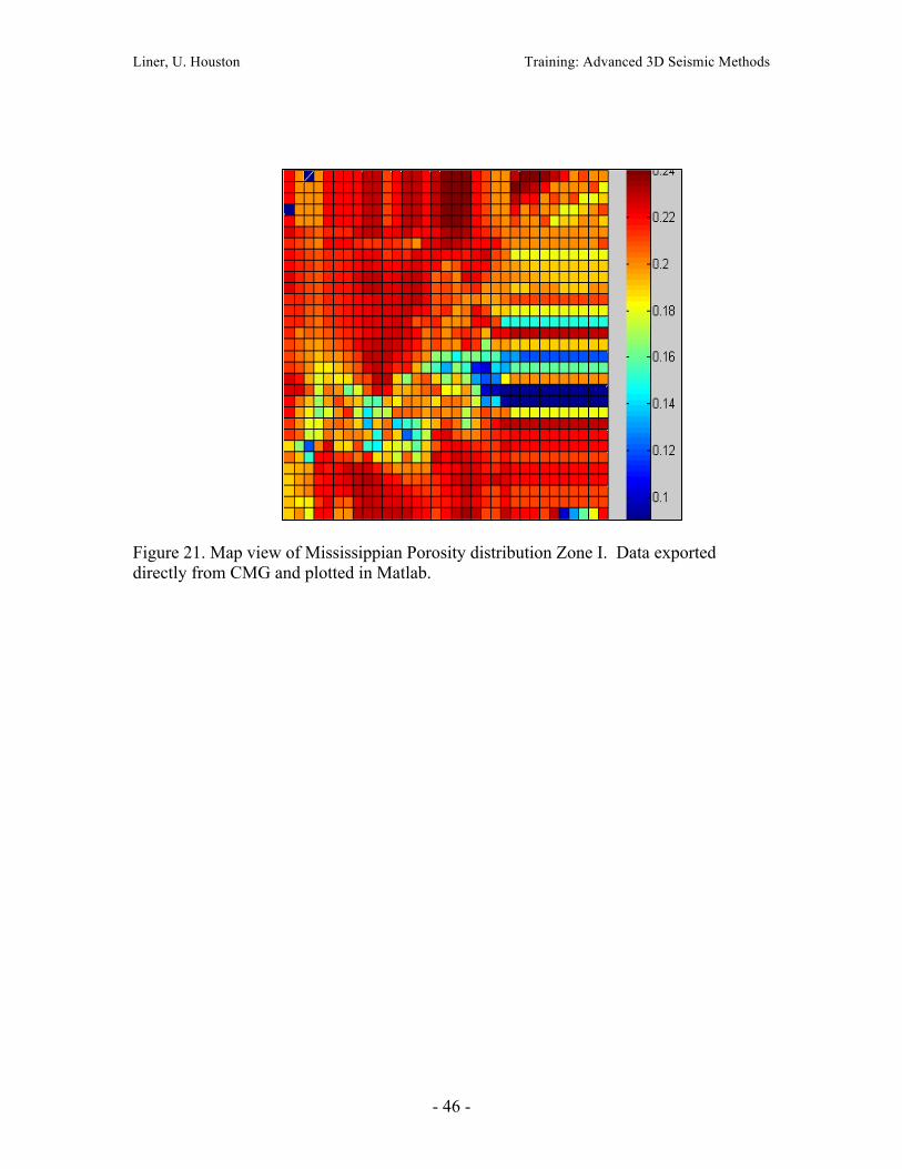
Figure 21. Map view of Mississippian Porosity distribution Zone I. Data exported directly from CMG and plotted in Matlab.


- 47 -

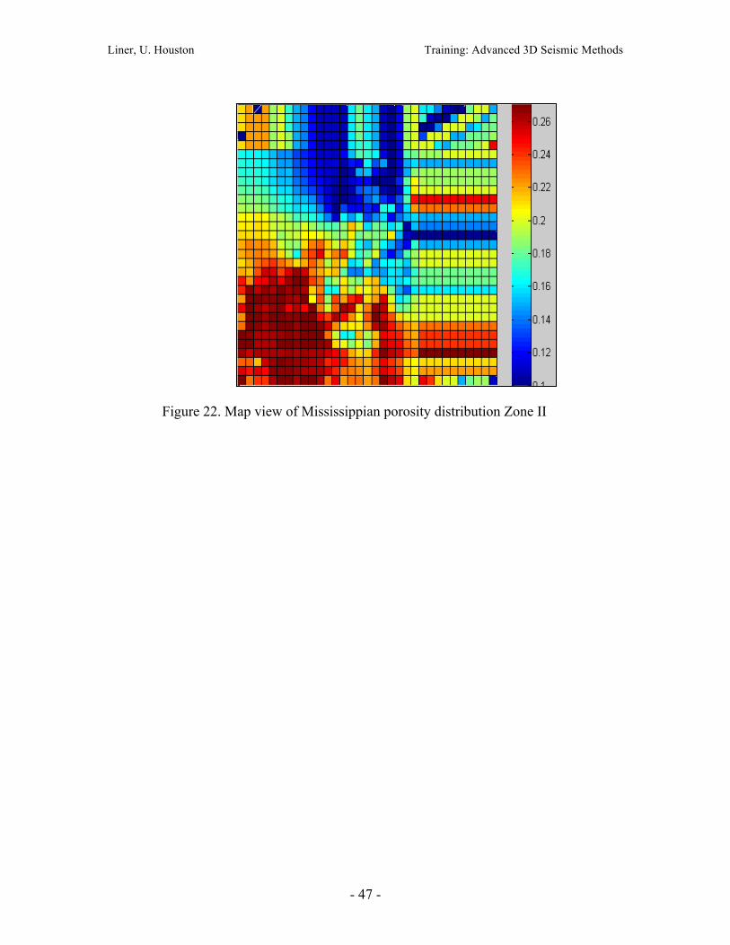
Figure 22. Map view of Mississippian porosity distribution Zone II


- 48 -

Figure 23. Reflection coefficients between Miss. zones I and II.


- 49 -

Figure 24: Time structure map of the top of the Mississippian unconformity pointing out the channel in the southeast corner.


- 50 -

Figure 25: Time slice at 0.85 seconds pointing out the channel feature in figure 24 correlates with the bright amplitudes in the time slice.


- 51 -

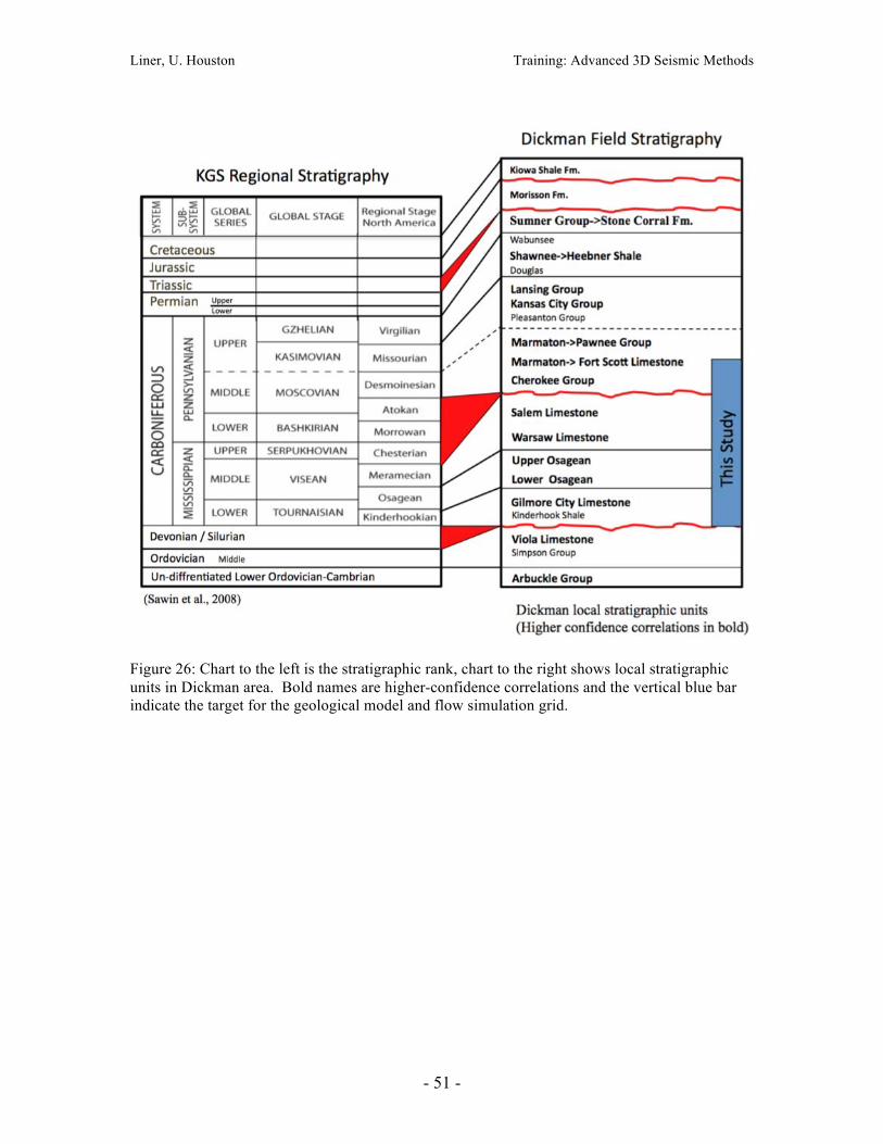
Figure 26: Chart to the left is the stratigraphic rank, chart to the right shows local stratigraphic units in Dickman area. Bold names are higher-confidence correlations and the vertical blue bar indicate the target for the geological model and flow simulation grid.


- 52 -

Figure 27: CO2 phase diagram (Leitner, 2000)


- 53 -

Figure 28: Deep penetration in Dickman area. (1) Humphrey 4-18 [TD in Viola], (2) Stiawalt 3 [Viola] , (3) Schaben 4 [Gilmore City], (4) Sidebottom 6 [Viola].


- 54 -

Figure 29: Synthetic on crossline 80 (left), note edge effects. Wavelet extraction polygon chosen to avoid edge effects (right).


- 55 -

Figure 30: Example of amplitude and the Spice attribute at the Dickman Field. Mississippian unconformity marked in red on Spice data (Liner, Flynn and Zeng, 2010)


- 56 -

Documents

Training toward Advanced 3D Seismic Methods for CO2 ... Monitoring, Verification, and Accounting ... codes from Seismic Unix are ... functionality we can test the effect of various