Embed Size (px)
Citation preview
CHAPTER 11. INTRODUCTION TO GEOMETRIC DESIGN NPTEL May 24, 2006
Chapter 11
Introduction to geometric design
11.1 Overview
The geometric design of highways deals with the dimensions and layout of visible features of the highway.
The emphasis of the geometric design is to address the requirement of the driver and the vehicle such as
safety, comfort, efficiency, etc. The features normally considered are the cross section elements, sight distance
consideration, horizontal curvature, gradients, and intersection. The design of these features is to a great
extend influenced by driver behavior and psychology, vehicle characteristics, traffic characteristics such as speed
and volume. Proper geometric design will help in the reduction of accidents and their severity. Therefore,
the objective of geometric design is to provide optimum efficiency in traffic operation and maximum safety at
reasonable cost. The planning cannot be done stage wise like that of a pavement, but has to be done well in
advance. The main components that will be discussed are:
1. Factors affecting the geometric design,
2. Highway alignment, road classification,
3. Pavement surface characteristics,
4. Cross-section elements including cross slope, various widths of roads and features in the road margins.
5. Sight distance elements including cross slope, various widths and features in the road margins.
6. Horizontal alignment which includes features like super elevation, transition curve, extra widening and set
back distance.
7. Vertical alignment and its components like gradient, sight distance and design of length of curves.
8. Intersection features like layout, capacity, etc.
11.2 Factors affecting geometric design
A number of factors affect the geometric design and they are discussed in detail in the following sections.
Introduction to Transportation Engineering 11.1 Tom V. Mathew and K V Krishna Rao
CHAPTER 11. INTRODUCTION TO GEOMETRIC DESIGN NPTEL May 24, 2006
11.2.1 Design speed
Design speed is the single most important factor that affects the geometric design. It directly affects the sight
distance, horizontal curve, and the length of vertical curves. Since the speed of vehicles vary with driver, terrain
etc, a design speed is adopted for all the geometric design.
Design speed is defined as the highest continuous speed at which individual vehicles can travel with safety
on the highway when weather conditions are conducive. Design speed is different from the legal speed limit
which is the speed limit imposed to curb a common tendency of drivers to travel beyond an accepted safe speed.
Design speed is also different from the desired speed which is the maximum speed at which a driver would travel
when unconstrained by either traffic or local geometry.
Since there are wide variations in the speed adopted by different drivers, and by different types of vehicles,
design speed should be selected such that it satisfy nearly all drivers. At the same time, a higher design speed
has cascading effect in other geometric design and thereby cost escalation. Therefore, an 85th percentile design
sped is normally adopted. This speed is defined as that speed which is greater than the speed of 85% of drivers.
In some countries this is as high as 95 to 98 percentile speed.
11.2.2 Topography
The next important factor that affects the geometric design is the topography. It is easier to construct roads
with required standards for a plain terrain. However, for a given design speed, the construction cost increases
multiform with the gradient and the terrain. Therefore, geometric design standards are different for different
terrain to keep the cost of construction and time of construction under control. This is characterized by sharper
curves and steeper gradients.
11.2.3 Other factors
In addition to design speed and topography, there are various other factors that affect the geometric design and
they are briefly discussed below:
• Vehicle: :The dimensions, weight of the axle and operating characteristics of a vehicle influence the design
aspects such as width of the pavement, radii of the curve, clearances, parking geometrics etc. affects the
design. A design vehicle which has standard weight, dimensions and operating characteristics are used to
establish highway design controls to accommodate vehicles of a designated type.
• Human: The important human factors that influences geometric design are the physical, mental and
psychological characteristics of the driver and pedestrians like the reaction time.
• Traffic: It will be uneconomical to design the road for peak traffic flow. Therefore a reasonable value of
traffic volume is selected as the design hourly volume which is determined from the various traffic data
collected. The geometric design is thus based on this design volume, capacity etc.
• Environmental: Factors like air pollution, noise pollution etc. should be given due consideration in the
geometric design of roads.
• Economy: The design adopted should be economical as far as possible. It should match with the funds
alloted for capital cost and maintenance cost.
• Others: Geometric design should be such that the aesthetics of the region is not affected.
Introduction to Transportation Engineering 11.2 Tom V. Mathew and K V Krishna Rao
CHAPTER 11. INTRODUCTION TO GEOMETRIC DESIGN NPTEL May 24, 2006
We will discuss on alignment, classification and factors affecting GD.
11.3 Road classification
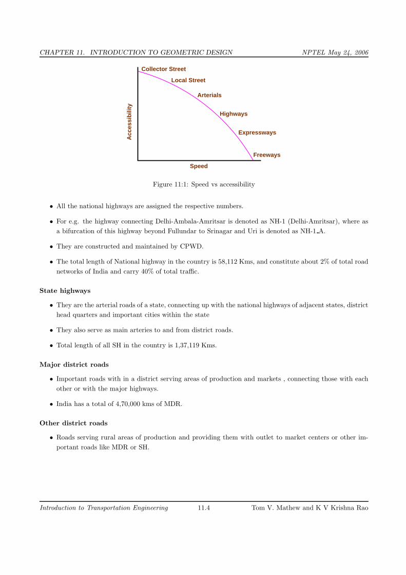
The roads can be classified in many ways. The classification based on speed and accessibility is the most generic
one. Note that as the accessibility of road increases, the speed reduces. (See figure 11:1). Accordingly, the
roads can classified as follows in the order of increased accessibility and reduced speeds.
• Freeways: Freeways are access controlled divided highways. Most freeways are four lanes, two lanes
each direction, but many freeways widen to incorporate more lanes as they enter urban areas. Access
is controlled through the use of interchanges, and the type of interchange depends upon the kind of
intersecting road way (rural roads, another freeway etc.)
• Expressways: They are superior type of highways and are designed for high speeds ( 120 km/hr is common),
high traffic volume and safety. They are generally provided with grade separations at intersections.
Parking, loading and unloading of goods and pedestrian traffic is not allowed on expressways.
• Highways: They represent the superior type of roads in the country. Highways are of two types - rural
highways and urban highways. Rural highways are those passing through rural areas (villages) and urban
highways are those passing through large cities and towns, ie. urban areas.
• Arterials: It is a general term denoting a street primarily meant for through traffic usually on a continuous
route. They are generally divided highways with fully or partially controlled access. Parking, loading
and unloading activities are usually restricted and regulated. Pedestrians are allowed to cross only at
intersections/designated pedestrian crossings.
• Local streets : A local street is the one which is primarily intended for access to residence, business or
abutting property. It does not normally carry large volume of traffic and also it allows unrestricted parking
and pedestrian movements.
• Collectors streets: These are streets intended for collecting and distributing traffic to and from local streets
and also for providing access to arterial streets. Normally full access is provided on these streets . There
are few parking restrictions except during peak hours.
11.3.1 Nagpur classification
In Nagpur road classification, all roads were classified into five categories as National highways, State highways,
Major district roads, Other district roads and village roads.
National highways
• They are main highways running through the length and breadth of India connecting major ports ,
foreign highways, capitals of large states and large industrial and tourist centers including roads required
for strategic movements.
• It was recommended by Jayakar committee that the National highways should be the frame on which the
entire road communication should be based.
Introduction to Transportation Engineering 11.3 Tom V. Mathew and K V Krishna Rao
CHAPTER 11. INTRODUCTION TO GEOMETRIC DESIGN NPTEL May 24, 2006
Speed
Highways
Expressways
Freeways
Arterials
Local Street
Collector Street
Acc
essi
bili
ty
Figure 11:1: Speed vs accessibility
• All the national highways are assigned the respective numbers.
• For e.g. the highway connecting Delhi-Ambala-Amritsar is denoted as NH-1 (Delhi-Amritsar), where as
a bifurcation of this highway beyond Fullundar to Srinagar and Uri is denoted as NH-1 A.
• They are constructed and maintained by CPWD.
• The total length of National highway in the country is 58,112 Kms, and constitute about 2% of total road
networks of India and carry 40% of total traffic.
State highways
• They are the arterial roads of a state, connecting up with the national highways of adjacent states, district
head quarters and important cities within the state
• They also serve as main arteries to and from district roads.
• Total length of all SH in the country is 1,37,119 Kms.
Major district roads
• Important roads with in a district serving areas of production and markets , connecting those with each
other or with the major highways.
• India has a total of 4,70,000 kms of MDR.
Other district roads
• Roads serving rural areas of production and providing them with outlet to market centers or other im-
portant roads like MDR or SH.
Introduction to Transportation Engineering 11.4 Tom V. Mathew and K V Krishna Rao
CHAPTER 11. INTRODUCTION TO GEOMETRIC DESIGN NPTEL May 24, 2006
Village roads
• They are roads connecting villages or group of villages with each other or to the nearest road of a higher
category like ODR or MDR.
• India has 26,50,000 kms of ODR+VR out of the total 33,15,231 kms of all type of roads.
11.3.2 Modern-Lucknow classification
The roads in the country were classified into 3 classes:
Primary roads
• Expressways
• National highways
Secondary roads
• State highways
• Major district roads
Tertiary roads
• Other district roads
• Village roads
11.3.3 Roads classification criteria
Apart from the classification given by the different plans, roads were also classified based on some other criteria.
They are given in detail below.
Based on usage
This classification is based on whether the roads can be used during different seasons of the year.
• All-weather roads: Those roads which are negotiable during all weathers, except at major river crossings
where interruption of traffic is permissible up to a certain extent are called all weather roads.
• Fair-weather roads: Roads which are negotiable only during fair weather are called fair weather roads.
Based on carriage way
This classification is based on the type of the carriage way or the road pavement.
• Paved roads with hards surface : If they are provided with a hard pavement course such roads are called
paved roads.(eg: stones, Water bound macadam (WBM), Bituminous macadam (BM), concrete roads)
• Unpaved roads: Roads which are not provided with a hard course of atleast a WBM layer they is called
unpaved roads. Thus earth and gravel roads come under this category.
Introduction to Transportation Engineering 11.5 Tom V. Mathew and K V Krishna Rao
CHAPTER 11. INTRODUCTION TO GEOMETRIC DESIGN NPTEL May 24, 2006
Based on pavement surface
Based on the type of pavement surfacing provided, they are classified as surfaced and unsurfaced roads.
• Surfaced roads (BM, concrete): Roads which are provided with a bituminous or cement concreting surface
are called surfaced roads.
• Unsurfaced roads (soil/gravel): Roads which are not provided with a bituminous or cement concreting
surface are called unsurfaced roads.
Other criteria
Roads may also be classified based on the traffic volume in that road, load transported through that road, or
location and function of that road.
• Traffic volume : Based on the traffic volume, they are classified as heavy, medium and light traffic roads.
These terms are relative and so the limits under each class may be expressed as vehicles per day.
• Load transported : Based on the load carried by these roads, they can be classified as class I, class II, etc.
or class A, class B etc. and the limits may be expressed as tonnes per day.
• Location and function : The classification based on location and function should be a more acceptable
classification since they may be defined clearly. Classification of roads by Nagpur Road plan is based on
the location and function which we had seen earlier.
11.4 Highway alignment
Once the necessity of the highway is assessed, the next process is deciding the alignment. The highway alignment
can be either horizontal or vertical and they are described in detail in the following sections.
11.4.1 Alignment
The position or the layout of the central line of the highway on the ground is called the alignment. Horizontal
alignment includes straight and curved paths. Vertical alignment includes level and gradients. Alignment
decision is important because a bad alignment will enhance the construction, maintenance and vehicle operating
cost. Once an alignment is fixed and constructed, it is not easy to change it due to increase in cost of adjoining
land and construction of costly structures by the roadside.
11.4.2 Requirements
The requirements of an ideal alignment are
• The alignment between two terminal stations should be short and as far as possible be straight, but due
to some practical considerations deviations may be needed.
• The alignment should be easy to construct and maintain. It should be easy for the operation of vehicles.
So to the maximum extend easy gradients and curves should be provided.
Introduction to Transportation Engineering 11.6 Tom V. Mathew and K V Krishna Rao
CHAPTER 11. INTRODUCTION TO GEOMETRIC DESIGN NPTEL May 24, 2006
• It should be safe both from the construction and operating point of view especially at slopes, embankments,
and cutting.It should have safe geometric features.
• The alignment should be economical and it can be considered so only when the initial cost, maintenance
cost, and operating cost is minimum.
11.4.3 Factors controlling alignment
We have seen the requirements of an alignment. But it is not always possible to satisfy all these requirements.
Hence we have to make a judicial choice considering all the factors.
The various factors that control the alignment are as follows:
• obligatory points These are the control points governing the highway alignment. These points are classified
into two categories. Points through which it should pass and points through which it should not pass.
Some of the examples are:
– bridge site: The bridge can be located only where the river has straight and permanent path and
also where the abutment and pier can be strongly founded. The road approach to the bridge should
not be curved and skew crossing should be avoided as possible. Thus to locate a bridge the highway
alignment may be changed.
– mountain: While the alignment passes through a mountain, the various alternatives are to either
construct a tunnel or to go round the hills. The suitability of the alternative depends on factors like
topography, site conditions and construction and operation cost.
– intermediate town: The alignment may be slightly deviated to connect an intermediate town or
village nearby.
These were some of the obligatory points through which the alignment should pass. Coming to the second
category, that is the points through which the alignment should not pass are:
– religious places: These have been protected by the law from being acquired for any purpose.Therefore,
these points should be avoided while aligning.
– very costly structures: Acquiring such structures means heavy compensation which would result in
an increase in initial cost. So the alignment may be deviated not to pass through that point.
– lakes/ponds etc: The presence of a lake or pond on the alignment path would also necessitate
deviation of the alignment.
• Traffic: The alignment should suit the traffic requirements. Based on the origin-destination data of the
area, the desire lines should be drawn. The new alignment should be drawn keeping in view the desire
lines, traffic flow pattern etc.
• Geometric design:Geometric design factors such as gradient, radius of curve, sight distance etc. also
governs the alignment of the highway. To keep the radius of curve minimum, it may be required to change
the alignment of the highway. The alignments should be finalized such that the obstructions to visibility
do not restrict the minimum requirements of sight distance. The design standards vary with the class of
road and the terrain and accordingly the highway should be aligned.
Introduction to Transportation Engineering 11.7 Tom V. Mathew and K V Krishna Rao
CHAPTER 11. INTRODUCTION TO GEOMETRIC DESIGN NPTEL May 24, 2006
• Economy:The alignment finalised should be economical. All the three costs i.e. construction, maintenance,
and operating cost should be minimum. The construction cost can be decreased much if it is possible to
maintain a balance between cutting and filling. Also try to avoid very high embankments and very deep
cuttings as the construction cost will be very higher in these cases.
• Other considerations : various other factors that govern the alignment are drainage considerations, political
factors and monotony.
– Drainage:
– Political: If a foreign territory comes across a straight alignment, we will have to deviate the alignment
around the foreign land.
– Monotony: For a flat terrain it is possible to provide a straight alignment, but it will be monotonous
for driving. Hence a slight bend may be provided after a few kilometres of straight road to keep the
driver alert by breaking the monotony.
– Hydrological (rainfall/water table):
11.4.4 Special consideration for hilly areas
Alignment through hilly areas is slightly different from aligning through a flat terrain. For the purpose of
efficient and safe operation of vehicles through a hilly terrain special care should be taken while aligning the
highway. Some of the special considerations for highway alignment through a hilly terrain is discussed below.
• Stability of the slopes: for hilly areas, the road should be aligned through the side of the hill that is
stable. The common problem with hilly areas is that of landslides. Excessive cutting and filling for road
constructions give way to steepening of slopes which in turn will affect the stability.
• Hill side drainage: Adequate drainage facility should be provided across the road. Attempts should be
made to align the roads in such a way where the number of cross drainage structures required are minimum.
This will reduce the construction cost.
• Special geometric standards: The geometric standards followed in hilly areas are different from those in
flat terrain. The alignment chosen should enable the ruling gradient to be attained in minimum of the
length, minimizing steep gradient, hairpin bends and needless rise and fall.
• Ineffective rise and fall : Efforts should be made to keep the ineffective rise and excessive fall minimum.
11.5 Summary
This lecture covers a brief history of highway engineering, highlighting the developments of road construction.
Significant among them are Roman, French, and British roads. British road construction practice developed by
Macadam is the most scientific and the present day roads follows this pattern. The highway development and
classification of Indian roads are also discussed. The major classes of roads include National Highway, State
highway, District roads, and Village roads. Finally, issues in highway alignment are discussed.
Introduction to Transportation Engineering 11.8 Tom V. Mathew and K V Krishna Rao
CHAPTER 11. INTRODUCTION TO GEOMETRIC DESIGN NPTEL May 24, 2006
11.6 Problems
1. Approximate length of National highway in India is:
(a) 1000 km
(b) 5000 km
(c) 10000 km
(d) 50000 km
(e) 100000 km
2. The most accessible road is
(a) National highway
(b) State highway
(c) Major District road
(d) Other District road
(e) Village road
11.7 Solutions
1. Approximate length of National highway in India is:
(a) 1000 km
(b) 5000 km
(c) 10000 km
(d) 50000 km
(e) 100000 km
2. The most accessible road is
(a) National highway
(b) State highway
(c) Major District road
(d) Other District road
(e) Village road√
Introduction to Transportation Engineering 11.9 Tom V. Mathew and K V Krishna Rao
CHAPTER 12. CROSS SECTIONAL ELEMENTS NPTEL May 24, 2006
Chapter 12
Cross sectional elements
12.1 Overview
The features of the cross-section of the pavement influences the life of the pavement as well as the riding comfort
and safety. Of these, pavement surface characteristics affect both of these. Camber,kerbs, and geometry of
various cross-sectional elements are important aspects to be considered in this regard. They are explained
briefly in this chapter.
12.2 Pavement surface characteristics
For a safe and comfortable driving four aspects of the pavement surface are important; the friction between the
wheels and the pavement surface, smoothness of the road surface, the light reflection characteristics of the top
of pavement surface, and drainage to water.
12.2.1 Friction
Friction between the wheel and the pavement surface is a crucial factor in the design of horizontal curves and
thus the safe operating speed. Further, it also affect the acceleration and deceleration ability of vehicles. Lack
of adequate friction can cause skidding or slipping of vehicles.
• Skidding happens when the path traveled along the road surface is more than the circumferential movement
of the wheels due to friction
• Slip occurs when the wheel revolves more than the corresponding longitudinal movement along the road.
Various factors that affect friction are:
• Type of the pavement (like bituminous, concrete, or gravel),
• Condition of the pavement (dry or wet, hot or cold, etc),
• Condition of the tyre (new or old), and
• Speed and load of the vehicle.
The frictional force that develops between the wheel and the pavement is the load acting multiplied by a factor
called the coefficient of friction and denoted as f . The choice of the value of f is a very complicated issue since
it depends on many variables. IRC suggests the coefficient of longitudinal friction as 0.35-0.4 depending on
Introduction to Transportation Engineering 12.1 Tom V. Mathew and K V Krishna Rao
CHAPTER 12. CROSS SECTIONAL ELEMENTS NPTEL May 24, 2006
the speed and coefficient of later friction as 0.15. The former is useful in sight distance calculation and the
latter in horizontal curve design.
12.2.2 Unevenness
It is always desirable to have an even surface, but it is seldom possible to have such one. Even if a road is
constructed with high quality pavers, it is possible to develop unevenness due to pavement failures. Unevenness
affect the vehicle operating cost, speed, riding comfort, safety, fuel consumption and wear and tear of tyres.
Unevenness index is a measure of unevenness which is the cumulative measure of vertical undulation of
the pavement surface recorded per unit horizontal length of the road. An unevenness index value less than 1500
mm/km is considered as good, a value less than 2500 mm.km is satisfactory up to speed of 100 kmph and values
greater than 3200 mm/km is considered as uncomfortable even for 55 kmph.
12.2.3 Light reflection
• White roads have good visibility at night, but caused glare during day time.
• Black roads has no glare during day, but has poor visibility at night
• Concrete roads has better visibility and less glare
It is necessary that the road surface should be visible at night and reflection of light is the factor that answers
it.
12.2.4 Drainage
The pavement surface should be absolutely impermeable to prevent seepage of water into the pavement layers.
Further,both the geometry and texture of pavement surface should help in draining out the water from the
surface in less time.
12.3 Camber
Camber or cant is the cross slope provided to raise middle of the road surface in the transverse direction to
drain off rain water from road surface. The objectives of providing camber are:
• Surface protection especially for gravel and bituminous roads
• Sub-grade protection by proper drainage
• Quick drying of pavement which in turn increases safety
Too steep slope is undesirable for it will erode the surface. Camber is measured in 1 in n or n% (Eg. 1 in 50 or
2%) and the value depends on the type of pavement surface. The values suggested by IRC for various categories
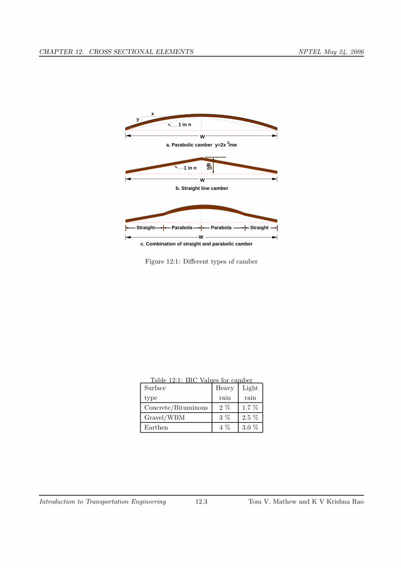
of pavement is given in Table 12:1 The common types of camber are parabolic, straight, or combination of them
(Figure 12:1)
Introduction to Transportation Engineering 12.2 Tom V. Mathew and K V Krishna Rao
CHAPTER 12. CROSS SECTIONAL ELEMENTS NPTEL May 24, 2006
StraightParabolaParabolaStraight
b. Straight line camber
a. Parabolic camber y=2x /nw
c. Combination of straight and parabolic camber
W
yx
1 in n
W
1 in nw2n
2
W
Figure 12:1: Different types of camber
Table 12:1: IRC Values for camberSurface Heavy Light
type rain rain
Concrete/Bituminous 2 % 1.7 %
Gravel/WBM 3 % 2.5 %
Earthen 4 % 3.0 %
Introduction to Transportation Engineering 12.3 Tom V. Mathew and K V Krishna Rao
CHAPTER 12. CROSS SECTIONAL ELEMENTS NPTEL May 24, 2006
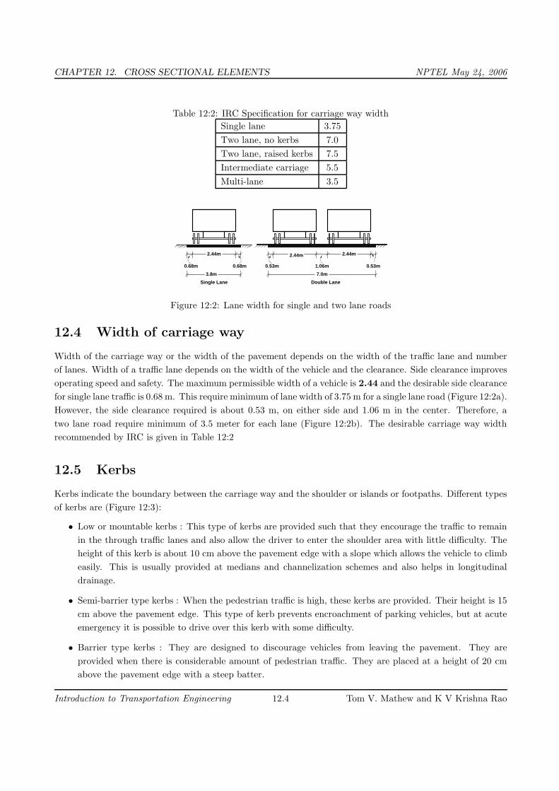
Table 12:2: IRC Specification for carriage way width
Single lane 3.75
Two lane, no kerbs 7.0
Two lane, raised kerbs 7.5
Intermediate carriage 5.5
Multi-lane 3.5
2.44m 2.44m2.44m
0.68m 0.68m 0.53m 1.06m 0.53m
3.8m 7.0m
Single Lane Double Lane
Figure 12:2: Lane width for single and two lane roads
12.4 Width of carriage way
Width of the carriage way or the width of the pavement depends on the width of the traffic lane and number
of lanes. Width of a traffic lane depends on the width of the vehicle and the clearance. Side clearance improves
operating speed and safety. The maximum permissible width of a vehicle is 2.44 and the desirable side clearance
for single lane traffic is 0.68 m. This require minimum of lane width of 3.75 m for a single lane road (Figure 12:2a).
However, the side clearance required is about 0.53 m, on either side and 1.06 m in the center. Therefore, a
two lane road require minimum of 3.5 meter for each lane (Figure 12:2b). The desirable carriage way width
recommended by IRC is given in Table 12:2
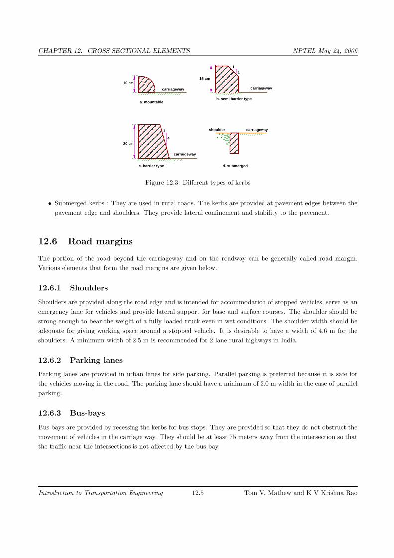
12.5 Kerbs
Kerbs indicate the boundary between the carriage way and the shoulder or islands or footpaths. Different types
of kerbs are (Figure 12:3):
• Low or mountable kerbs : This type of kerbs are provided such that they encourage the traffic to remain
in the through traffic lanes and also allow the driver to enter the shoulder area with little difficulty. The
height of this kerb is about 10 cm above the pavement edge with a slope which allows the vehicle to climb
easily. This is usually provided at medians and channelization schemes and also helps in longitudinal
drainage.
• Semi-barrier type kerbs : When the pedestrian traffic is high, these kerbs are provided. Their height is 15
cm above the pavement edge. This type of kerb prevents encroachment of parking vehicles, but at acute
emergency it is possible to drive over this kerb with some difficulty.
• Barrier type kerbs : They are designed to discourage vehicles from leaving the pavement. They are
provided when there is considerable amount of pedestrian traffic. They are placed at a height of 20 cm
above the pavement edge with a steep batter.
Introduction to Transportation Engineering 12.4 Tom V. Mathew and K V Krishna Rao
CHAPTER 12. CROSS SECTIONAL ELEMENTS NPTEL May 24, 2006
a. mountable
10 cm
carriageway
15 cm
carriageway
b. semi barrier type
carriagewayshoulder
c. barrier type d. submerged
carraigeway
20 cm
������������������������������������������������������������������
������������������������������������������������������������������
���������
������������������������������������������
������������������������������
���������������������������������������������
���������������������������������������������
������������������������������������������������������������������������������������������������������������������������
������������������������������������������������
���������������������������������������������������������������������������������������������������
�����������������������������������������������������������������������������������������������������������������������������������������������������������������������������������������������������������������
1
4
11
Figure 12:3: Different types of kerbs
• Submerged kerbs : They are used in rural roads. The kerbs are provided at pavement edges between the
pavement edge and shoulders. They provide lateral confinement and stability to the pavement.
12.6 Road margins
The portion of the road beyond the carriageway and on the roadway can be generally called road margin.
Various elements that form the road margins are given below.
12.6.1 Shoulders
Shoulders are provided along the road edge and is intended for accommodation of stopped vehicles, serve as an
emergency lane for vehicles and provide lateral support for base and surface courses. The shoulder should be
strong enough to bear the weight of a fully loaded truck even in wet conditions. The shoulder width should be
adequate for giving working space around a stopped vehicle. It is desirable to have a width of 4.6 m for the
shoulders. A minimum width of 2.5 m is recommended for 2-lane rural highways in India.
12.6.2 Parking lanes
Parking lanes are provided in urban lanes for side parking. Parallel parking is preferred because it is safe for
the vehicles moving in the road. The parking lane should have a minimum of 3.0 m width in the case of parallel
parking.
12.6.3 Bus-bays
Bus bays are provided by recessing the kerbs for bus stops. They are provided so that they do not obstruct the
movement of vehicles in the carriage way. They should be at least 75 meters away from the intersection so that
the traffic near the intersections is not affected by the bus-bay.
Introduction to Transportation Engineering 12.5 Tom V. Mathew and K V Krishna Rao
CHAPTER 12. CROSS SECTIONAL ELEMENTS NPTEL May 24, 2006
12.6.4 Service roads
Service roads or frontage roads give access to access controlled highways like freeways and expressways. They
run parallel to the highway and will be usually isolated by a separator and access to the highway will be provided
only at selected points. These roads are provided to avoid congestion in the expressways and also the speed of
the traffic in those lanes is not reduced.
12.6.5 Cycle track
Cycle tracks are provided in urban areas when the volume of cycle traffic is high Minimum width of 2 meter is
required, which may be increased by 1 meter for every additional track.
12.6.6 Footpath
Footpaths are exclusive right of way to pedestrians, especially in urban areas. They are provided for the safety
of the pedestrians when both the pedestrian traffic and vehicular traffic is high. Minimum width is 1.5 meter
and may be increased based on the traffic. The footpath should be either as smooth as the pavement or more
smoother than that to induce the pedestrian to use the footpath.
12.6.7 Guard rails
They are provided at the edge of the shoulder usually when the road is on an embankment. They serve to
prevent the vehicles from running off the embankment, especially when the height of the fill exceeds 3 m.
Various designs of guard rails are there. Guard stones painted in alternate black and white are usually used.
They also give better visibility of curves at night under headlights of vehicles.
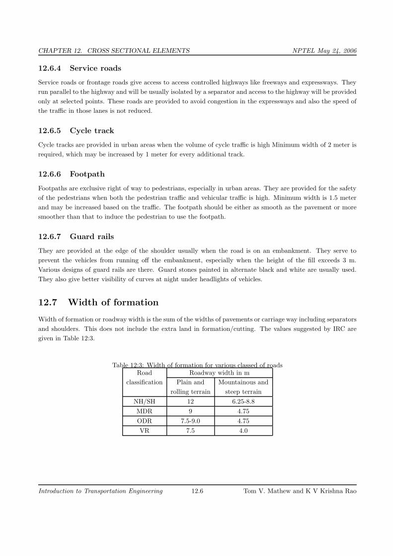
12.7 Width of formation
Width of formation or roadway width is the sum of the widths of pavements or carriage way including separators
and shoulders. This does not include the extra land in formation/cutting. The values suggested by IRC are
given in Table 12:3.
Table 12:3: Width of formation for various classed of roadsRoad Roadway width in m
classification Plain and Mountainous and
rolling terrain steep terrain
NH/SH 12 6.25-8.8
MDR 9 4.75
ODR 7.5-9.0 4.75
VR 7.5 4.0
Introduction to Transportation Engineering 12.6 Tom V. Mathew and K V Krishna Rao
CHAPTER 12. CROSS SECTIONAL ELEMENTS NPTEL May 24, 2006
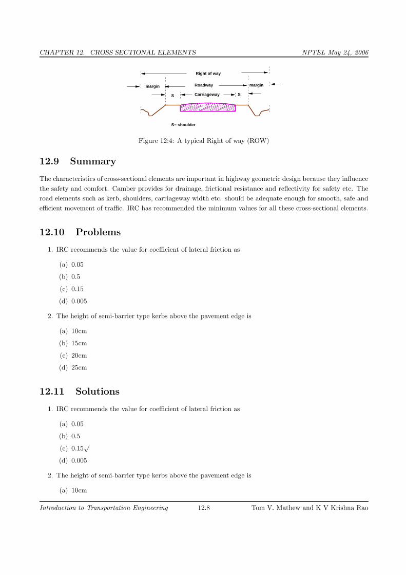
12.8 Right of way
Right of way (ROW) or land width is the width of land acquired for the road, along its alignment. It should
be adequate to accommodate all the cross-sectional elements of the highway and may reasonably provide for
future development. To prevent ribbon development along highways, control lines and building lines may be
provided. Control line is a line which represents the nearest limits of future uncontrolled building activity in
relation to a road. Building line represents a line on either side of the road, between which and the road no
building activity is permitted at all. The right of way width is governed by:
• Width of formation: It depends on the category of the highway and width of roadway and road margins.
• Height of embankment or depth of cutting: It is governed by the topography and the vertical alignment.
• Side slopes of embankment or cutting: It depends on the height of the slope, soil type etc.
• Drainage system and their size which depends on rainfall, topography etc.
• Sight distance considerations : On curves etc. there is restriction to the visibility on the inner side of the
curve due to the presence of some obstructions like building structures etc.
• Reserve land for future widening: Some land has to be acquired in advance anticipating future develop-
ments like widening of the road.
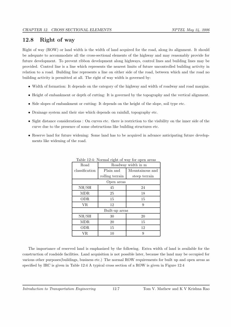
Table 12:4: Normal right of way for open areas
Road Roadway width in m
classification Plain and Mountainous and
rolling terrain steep terrain
Open areas
NH/SH 45 24
MDR 25 18
ODR 15 15
VR 12 9
Built-up areas
NH/SH 30 20
MDR 20 15
ODR 15 12
VR 10 9
The importance of reserved land is emphasized by the following. Extra width of land is available for the
construction of roadside facilities. Land acquisition is not possible later, because the land may be occupied for
various other purposes(buildings, business etc.) The normal ROW requirements for built up and open areas as
specified by IRC is given in Table 12:4 A typical cross section of a ROW is given in Figure 12:4
Introduction to Transportation Engineering 12.7 Tom V. Mathew and K V Krishna Rao
CHAPTER 12. CROSS SECTIONAL ELEMENTS NPTEL May 24, 2006
����������������������������������������������������������������������������������������������������������������������������
����������������������������������������������������������������������������������������������������������������������������
����������������������������������������������������������������������������������������������������������������������������
Carriageway SS
Roadwaymargin margin
Right of way
S− shoulder
Figure 12:4: A typical Right of way (ROW)
12.9 Summary
The characteristics of cross-sectional elements are important in highway geometric design because they influence
the safety and comfort. Camber provides for drainage, frictional resistance and reflectivity for safety etc. The
road elements such as kerb, shoulders, carriageway width etc. should be adequate enough for smooth, safe and
efficient movement of traffic. IRC has recommended the minimum values for all these cross-sectional elements.
12.10 Problems
1. IRC recommends the value for coefficient of lateral friction as
(a) 0.05
(b) 0.5
(c) 0.15
(d) 0.005
2. The height of semi-barrier type kerbs above the pavement edge is
(a) 10cm
(b) 15cm
(c) 20cm
(d) 25cm
12.11 Solutions
1. IRC recommends the value for coefficient of lateral friction as
(a) 0.05
(b) 0.5
(c) 0.15√
(d) 0.005
2. The height of semi-barrier type kerbs above the pavement edge is
(a) 10cm
Introduction to Transportation Engineering 12.8 Tom V. Mathew and K V Krishna Rao

CHAPTER 12. CROSS SECTIONAL ELEMENTS NPTEL May 24, 2006
(b) 15cm√
(c) 20cm
(d) 25cm
Introduction to Transportation Engineering 12.9 Tom V. Mathew and K V Krishna Rao
CHAPTER 13. SIGHT DISTANCE NPTEL May 24, 2006
Chapter 13
Sight distance
13.1 Overview
The safe and efficient operation of vehicles on the road depends very much on the visibility of the road ahead of
the driver. Thus the geometric design of the road should be done such that any obstruction on the road length
could be visible to the driver from some distance ahead . This distance is said to be the sight distance.
13.2 Types of sight distance
Sight distance available from a point is the actual distance along the road surface, over which a driver from
a specified height above the carriage way has visibility of stationary or moving objects. Three sight distance
situations are considered for design:
• Stopping sight distance (SSD) or the absolute minimum sight distance
• Intermediate sight distance (ISD) is the defined as twice SSD
• Overtaking sight distance (OSD) for safe overtaking operation
• Head light sight distance is the distance visible to a driver during night driving under the illumination of
head light
• Safe sight distance to enter into an intersection
The most important consideration in all these is that at all times the driver traveling at the design speed of
the highway must have sufficient carriageway distance within his line of vision to allow him to stop his vehicle
before colliding with a slowly moving or stationary object appearing suddenly in his own traffic lane.
The computation of sight distance depends on:
• Reaction time of the driver
Reaction time of a driver is the time taken from the instant the object is visible to the driver to the
instant when the brakes are applied. The total reaction time may be split up into four components based
on PIEV theory. In practice, all these times are usually combined into a total perception- reaction time
suitable fro design purposes as well as for easy measurement. Many of the studies shows that drivers
require about 1.5 to 2 secs under normal conditions. However taking into consideration the variability of
driver characteristics, a higher value is normally used in design. For example, IRC suggests a reaction
time of 2.5 secs.
Introduction to Transportation Engineering 13.1 Tom V. Mathew and K V Krishna Rao

CHAPTER 13. SIGHT DISTANCE NPTEL May 24, 2006
• Speed of the vehicle
The speed of the vehicle very much affects the sight distance. Higher the speed, more time will be required
to stop the vehicle. Hence it is evident that, as the speed increases, sight distance also increases.
• Efficiency of brakes
The efficiency of the brakes depends upon the age of the vehicle, vehicle characteristics etc. If the brake
efficiency is 100%, the vehicle will stop the moment the brakes are applied. But practically, it is not
possible to achieve 100% brake efficiency. Therefore it could be understood that sight distance required
will be more when the efficiency of brakes are less. Also for safe geometric design, we assume that the
vehicles have only 50% brake efficiency.
• Frictional resistance between the tyre and the road The frictional resistance between the tyre and road
plays an important role to bring the vehicle to stop. When the frictional resistance is more, the vehicles
stop immediately. Thus sight required will be less. No separate provision for brake efficiency is provided
while computing the sight distance. This is taken into account along with the factor of longitudinal
friction. IRC has specified the value of longitudinal friction in between 0.35 to 0.4.
• Gradient of the road. Gradient of the road also affects the sight distance. While climbing up a gradient,
the vehicle can stop immediately. Therefore sight distance required is less. While descending a gradient,
gravity also comes into action and more time will be required to stop the vehicle. Sight distance required
will be more in that case.
13.3 Stopping sight distance
SSD is the minimum sight distance available on a highway at any spot having sufficient length to enable the
driver to stop a vehicle traveling at design speed, safely without collision with any other obstruction.
There is a term called safe stopping distance and is one of the important measures in traffic engineering. It
is the distance a vehicle travels from the point at which a situation is first perceived to the time the deceleration
is complete. Drivers must have adequate time if they are to suddenly respond to a situation. Thus in a highway
design, a sight distance atleast equal to the safe stopping distance should be provided. The stopping sight
distance is the sum of lag distance and the braking distance. Lag distance is the distance the vehicle traveled
during the reaction time t and is given by vt, where v is the velocity in m/sec2. Braking distance is the distance
traveled by the vehicle during braking operation. For a level road this is obtained by equating the work done in
stopping the vehicle and the kinetic energy of the vehicle. If F is the maximum frictional force developed and
the braking distance is l, then work done against friction in stopping the vehicle is F l = fWl where W is the
total weight of the vehicle. The kinetic energy at the design speed is
1
2mv2 =
1
2
Wv2
g
fWl =Wv2
2g
l =v2
2gf
Therefore, the SSD = lag distance + braking distance and given by:
Introduction to Transportation Engineering 13.2 Tom V. Mathew and K V Krishna Rao
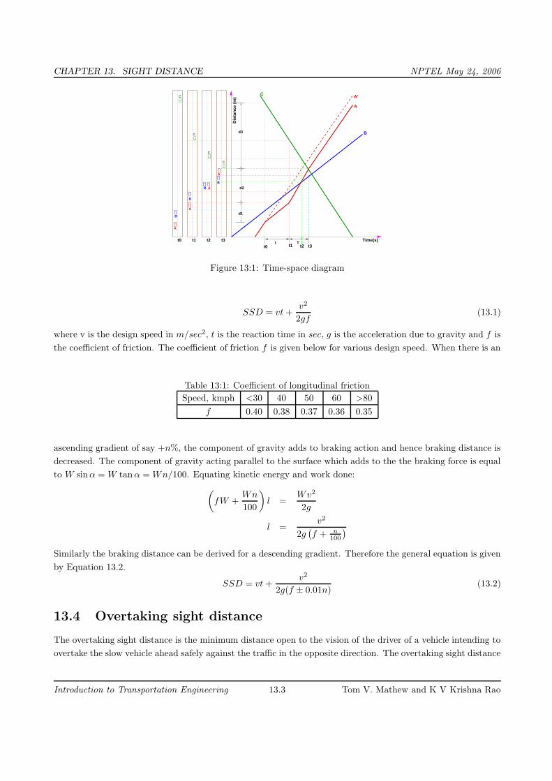
CHAPTER 13. SIGHT DISTANCE NPTEL May 24, 2006
t1 t2 t3t0
d1
d2
d3
C
B
A’
A
t1 t2 t3t0T
Time(s)D
ista
nce
(m)
B
B
B
A
A
A
A
B
C
C
C
C
t
Figure 13:1: Time-space diagram
SSD = vt +v2
2gf(13.1)
where v is the design speed in m/sec2, t is the reaction time in sec, g is the acceleration due to gravity and f is
the coefficient of friction. The coefficient of friction f is given below for various design speed. When there is an
Table 13:1: Coefficient of longitudinal friction
Speed, kmph <30 40 50 60 >80
f 0.40 0.38 0.37 0.36 0.35
ascending gradient of say +n%, the component of gravity adds to braking action and hence braking distance is
decreased. The component of gravity acting parallel to the surface which adds to the the braking force is equal
to W sin α = W tan α = Wn/100. Equating kinetic energy and work done:
(
fW +Wn
100
)
l =Wv2
2g
l =v2
2g(
f + n
100
)
Similarly the braking distance can be derived for a descending gradient. Therefore the general equation is given
by Equation 13.2.
SSD = vt +v2
2g(f ± 0.01n)(13.2)
13.4 Overtaking sight distance
The overtaking sight distance is the minimum distance open to the vision of the driver of a vehicle intending to
overtake the slow vehicle ahead safely against the traffic in the opposite direction. The overtaking sight distance
Introduction to Transportation Engineering 13.3 Tom V. Mathew and K V Krishna Rao
CHAPTER 13. SIGHT DISTANCE NPTEL May 24, 2006
t1 t2 t3t0
d1
d2
d3
C
B
A’
A
t1 t2 t3t0T
Time(s)D
ista
nce
(m)
B
B
B
A
A
A
A
B
C
C
C
C
t
Figure 13:2: Illustration of overtaking sight distance
or passing sight distance is measured along the center line of the road over which a driver with his eye level 1.2
m above the road surface can see the top of an object 1.2 m above the road surface.
The factors that affect the OSD are:
• Velocities of the overtaking vehicle, overtaken vehicle and of the vehicle coming in the opposite direction.
• Spacing between vehicles, which in-turn depends on the speed
• Skill and reaction time of the driver
• Rate of acceleration of overtaking vehicle
• Gradient of the road
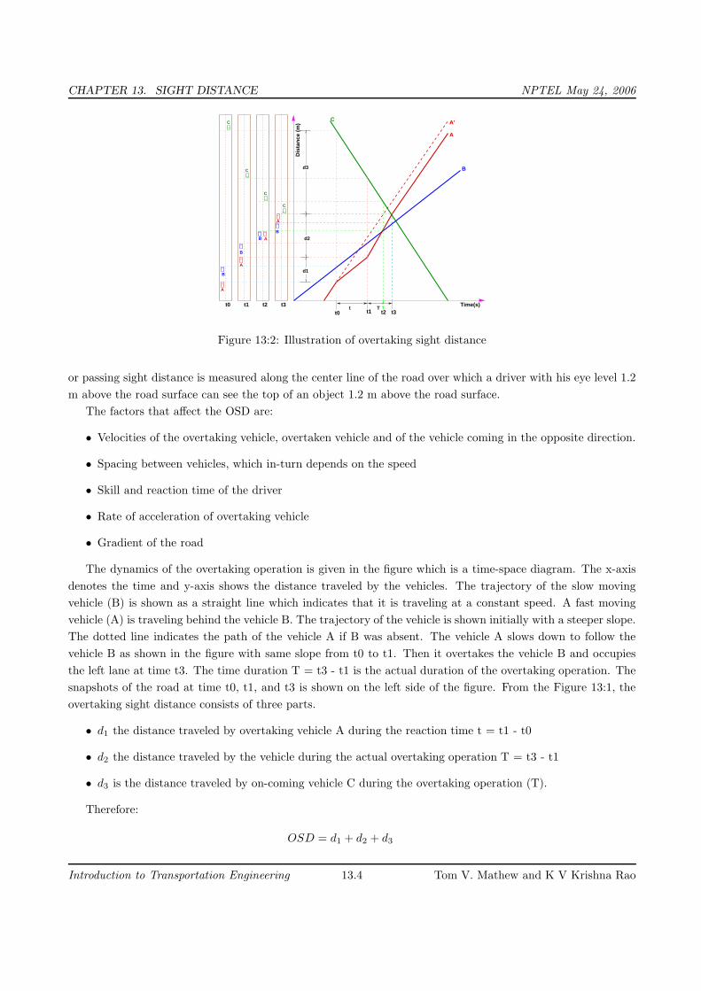
The dynamics of the overtaking operation is given in the figure which is a time-space diagram. The x-axis
denotes the time and y-axis shows the distance traveled by the vehicles. The trajectory of the slow moving
vehicle (B) is shown as a straight line which indicates that it is traveling at a constant speed. A fast moving
vehicle (A) is traveling behind the vehicle B. The trajectory of the vehicle is shown initially with a steeper slope.
The dotted line indicates the path of the vehicle A if B was absent. The vehicle A slows down to follow the
vehicle B as shown in the figure with same slope from t0 to t1. Then it overtakes the vehicle B and occupies
the left lane at time t3. The time duration T = t3 - t1 is the actual duration of the overtaking operation. The
snapshots of the road at time t0, t1, and t3 is shown on the left side of the figure. From the Figure 13:1, the
overtaking sight distance consists of three parts.
• d1 the distance traveled by overtaking vehicle A during the reaction time t = t1 - t0
• d2 the distance traveled by the vehicle during the actual overtaking operation T = t3 - t1
• d3 is the distance traveled by on-coming vehicle C during the overtaking operation (T).
Therefore:
OSD = d1 + d2 + d3
Introduction to Transportation Engineering 13.4 Tom V. Mathew and K V Krishna Rao
CHAPTER 13. SIGHT DISTANCE NPTEL May 24, 2006
It is assumed that the vehicle A is forced to reduce its speed to vb, the speed of the slow moving vehicle B and
travels behind it during the reaction time t of the driver. So d1 is given by:
d1 = vbt
Then the vehicle A starts to accelerate, shifts the lane, overtake and shift back to the original lane. The vehicle
A maintains the spacing s before and after overtaking. The spacing s in m is given by:
s = 0.7vb + 6 (13.3)
Let T be the duration of actual overtaking. The distance traveled by B during the overtaking operation is
2s+vbT . Also, during this time, vehicle A accelerated from initial velocity vb and overtaking is completed while
reaching final velocity v. Hence the distance traveled is given by:
d2 = vbT +1
2aT 2
2s + vbT = vbT +1
2aT 2
2s =1
2aT 2
T =
√
4s
a
d2 = 2s + vb
√
4s
a
The distance traveled by the vehicle C moving at design speed v m/sec during overtaking operation is given by:
d3 = vT
The the overtaking sight distance is (Figure 13:1)
OSD = vbt + 2s + vb
√
4s
a+ vT (13.4)
where vb is the velocity of the slow moving vehicle in m/sec2, t the reaction time of the driver in sec, s is the
spacing between the two vehicle in m given by equation 13.3 and a is the overtaking vehicles acceleration in
m/sec2. In case the speed of the overtaken vehicle is not given, it can be assumed that it moves 16 kmph slower
the the design speed.
The acceleration values of the fast vehicle depends on its speed and given in Table 13:2. Note that:
• On divided highways, d3 need not be considered
• On divided highways with four or more lanes, IRC suggests that it is not necessary to provide the OSD,
but only SSD is sufficient.
Overtaking zones
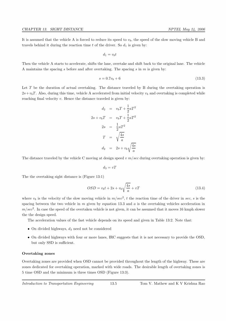
Overtaking zones are provided when OSD cannot be provided throughout the length of the highway. These are
zones dedicated for overtaking operation, marked with wide roads. The desirable length of overtaking zones is
5 time OSD and the minimum is three times OSD (Figure 13:3).
Introduction to Transportation Engineering 13.5 Tom V. Mathew and K V Krishna Rao
CHAPTER 13. SIGHT DISTANCE NPTEL May 24, 2006
Table 13:2: Maximum overtaking acceleration at different speeds
Speed Maximum overtaking
(kmph) acceleration (m/sec2)
25 1.41
30 1.30
40 1.24
50 1.11
65 0.92
80 0.72
100 0.53
S2−−End of Overtaking zoneS1−− Overtaking zone begin
3−5 times osd
osdosd
osd
3−5 times osd
osd
S1
S2
S2S1
Figure 13:3: Overtaking zones
13.5 Sight distance at intersections
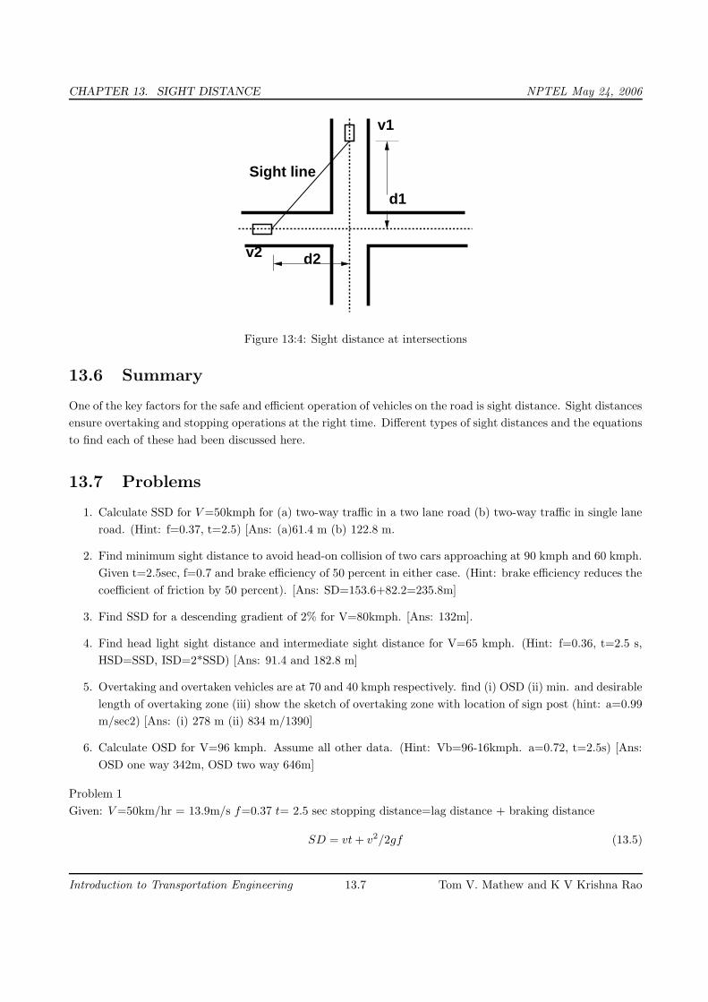
At intersections where two or more roads meet, visibility should be provided for the drivers approaching the
intersection from either sides. They should be able to perceive a hazard and stop the vehicle if required. Stopping
sight distance for each road can be computed from the design speed. The sight distance should be provided
such that the drivers on either side should be able to see each other. This is illustrated in the figure 13:4 Design
of sight distance at intersections may be used on three possible conditions:
• Enabling approaching vehicle to change the speed
• Enabling approaching vehicle to stop
• Enabling stopped vehicle to cross a main road
Introduction to Transportation Engineering 13.6 Tom V. Mathew and K V Krishna Rao
CHAPTER 13. SIGHT DISTANCE NPTEL May 24, 2006
v2
d1
v1
d2
Sight line
Figure 13:4: Sight distance at intersections
13.6 Summary
One of the key factors for the safe and efficient operation of vehicles on the road is sight distance. Sight distances
ensure overtaking and stopping operations at the right time. Different types of sight distances and the equations
to find each of these had been discussed here.
13.7 Problems
1. Calculate SSD for V =50kmph for (a) two-way traffic in a two lane road (b) two-way traffic in single lane
road. (Hint: f=0.37, t=2.5) [Ans: (a)61.4 m (b) 122.8 m.
2. Find minimum sight distance to avoid head-on collision of two cars approaching at 90 kmph and 60 kmph.
Given t=2.5sec, f=0.7 and brake efficiency of 50 percent in either case. (Hint: brake efficiency reduces the
coefficient of friction by 50 percent). [Ans: SD=153.6+82.2=235.8m]
3. Find SSD for a descending gradient of 2% for V=80kmph. [Ans: 132m].
4. Find head light sight distance and intermediate sight distance for V=65 kmph. (Hint: f=0.36, t=2.5 s,
HSD=SSD, ISD=2*SSD) [Ans: 91.4 and 182.8 m]
5. Overtaking and overtaken vehicles are at 70 and 40 kmph respectively. find (i) OSD (ii) min. and desirable
length of overtaking zone (iii) show the sketch of overtaking zone with location of sign post (hint: a=0.99
m/sec2) [Ans: (i) 278 m (ii) 834 m/1390]
6. Calculate OSD for V=96 kmph. Assume all other data. (Hint: Vb=96-16kmph. a=0.72, t=2.5s) [Ans:
OSD one way 342m, OSD two way 646m]
Problem 1
Given: V =50km/hr = 13.9m/s f=0.37 t= 2.5 sec stopping distance=lag distance + braking distance
SD = vt + v2/2gf (13.5)
Introduction to Transportation Engineering 13.7 Tom V. Mathew and K V Krishna Rao
CHAPTER 13. SIGHT DISTANCE NPTEL May 24, 2006
Stopping Distance = 61.4 m
Stopping sight distance when there are two lanes = stopping distance= 61.4m.
Stopping sight distance for a two way traffic for a single lane = 2[stopping distance]=122.8m
Problem 2 Given: V1 =90 Km/hr. V2 = 60 Km/hr. t = 2.5sec. Braking efficiency=50%. f=.7.
Stopping distance for one of the cars
SD = vt + v2/2gf (13.6)
Coefficient of friction due to braking efficiency of 50% = 0.5*0.7=0.35. Stopping sight distance of first car=
SD1= 153.6m
Stopping sight distance of second car= SD2= 82.2m
Stopping sight distance to avoid head on collision of the two approaching cars SD1+ SD2=235.8m.
Problem 3
Given: Gradient(n) = -2V = 80 Km/hr.
SD = vt + v2/2g(f − n (13.7)
SSD on road with gradient = 132m.
Problem 4
Given: V =65km/hr f=0.36 t= 2.5 sec
SD = vt + v2/2gf (13.8)
Headlight Sight distance = 91.4m.
Intermediate Sight distance= 2[SSD]= 182.8m.
Introduction to Transportation Engineering 13.8 Tom V. Mathew and K V Krishna Rao
CHAPTER 14. HORIZONTAL ALIGNMENT I NPTEL May 24, 2006
Chapter 14
Horizontal alignment I
14.1 Overview
Horizontal alignment is one of the most important features influencing the efficiency and safety of a highway. A
poor design will result in lower speeds and resultant reduction in highway performance in terms of safety and
comfort. In addition, it may increase the cost of vehicle operations and lower the highway capacity. Horizontal
alignment design involves the understanding on the design aspects such as design speed and the effect of
horizontal curve on the vehicles. The horizontal curve design elements include design of super elevation, extra
widening at horizontal curves, design of transition curve, and set back distance. These will be discussed in this
chapter and the following two chapters.
14.2 Design Speed
The design speed as noted earlier, is the single most important factor in the design of horizontal alignment. The
design speed also depends on the type of the road. For e.g, the design speed expected from a National highway
will be much higher than a village road, and hence the curve geometry will vary significantly.
The design speed also depends on the type of terrain. A plain terrain can afford to have any geometry, but
for the same standard in a hilly terrain requires substantial cutting and filling implying exorbitant costs as well
as safety concern due to unstable slopes. Therefore, the design speed is normally reduced for terrains with steep
slopes.
For instance, Indian Road Congress (IRC) has classified the terrains into four categories, namely plain,
rolling, mountainous, and steep based on the cross slope as given in table 14:1. Based on the type of road and
type of terrain the design speed varies. The IRC has suggested desirable or ruling speed as well as minimum
suggested design speed and is tabulated in table 14:2. The recommended design speed is given in Table 14:2.
Table 14:1: Terrain classificationTerrain classification Cross slope (%)
Plain 0-10
Rolling 10-25
Mountainous 25-60
Steep > 60
Introduction to Transportation Engineering 14.1 Tom V. Mathew and K V Krishna Rao
CHAPTER 14. HORIZONTAL ALIGNMENT I NPTEL May 24, 2006
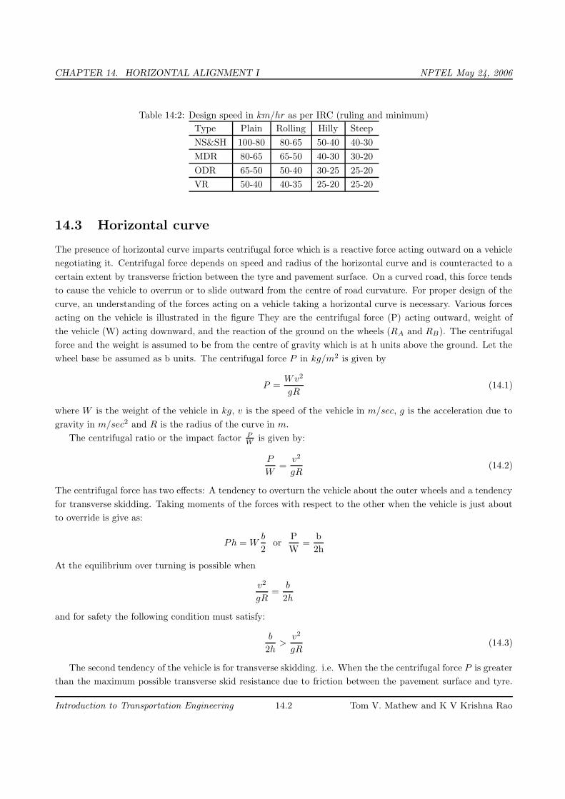
Table 14:2: Design speed in km/hr as per IRC (ruling and minimum)
Type Plain Rolling Hilly Steep
NS&SH 100-80 80-65 50-40 40-30
MDR 80-65 65-50 40-30 30-20
ODR 65-50 50-40 30-25 25-20
VR 50-40 40-35 25-20 25-20
14.3 Horizontal curve
The presence of horizontal curve imparts centrifugal force which is a reactive force acting outward on a vehicle
negotiating it. Centrifugal force depends on speed and radius of the horizontal curve and is counteracted to a
certain extent by transverse friction between the tyre and pavement surface. On a curved road, this force tends
to cause the vehicle to overrun or to slide outward from the centre of road curvature. For proper design of the
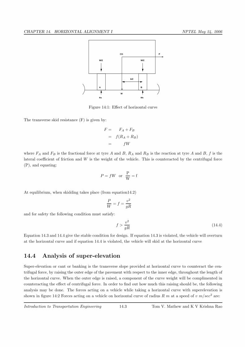
curve, an understanding of the forces acting on a vehicle taking a horizontal curve is necessary. Various forces
acting on the vehicle is illustrated in the figure They are the centrifugal force (P) acting outward, weight of
the vehicle (W) acting downward, and the reaction of the ground on the wheels (RA and RB). The centrifugal
force and the weight is assumed to be from the centre of gravity which is at h units above the ground. Let the
wheel base be assumed as b units. The centrifugal force P in kg/m2 is given by
P =Wv2
gR(14.1)
where W is the weight of the vehicle in kg, v is the speed of the vehicle in m/sec, g is the acceleration due to
gravity in m/sec2 and R is the radius of the curve in m.
The centrifugal ratio or the impact factor P
Wis given by:
P
W=
v2
gR(14.2)
The centrifugal force has two effects: A tendency to overturn the vehicle about the outer wheels and a tendency
for transverse skidding. Taking moments of the forces with respect to the other when the vehicle is just about
to override is give as:
Ph = Wb
2or
P
W=
b
2h
At the equilibrium over turning is possible when
v2
gR=
b
2h
and for safety the following condition must satisfy:
b
2h>
v2
gR(14.3)
The second tendency of the vehicle is for transverse skidding. i.e. When the the centrifugal force P is greater
than the maximum possible transverse skid resistance due to friction between the pavement surface and tyre.
Introduction to Transportation Engineering 14.2 Tom V. Mathew and K V Krishna Rao
CHAPTER 14. HORIZONTAL ALIGNMENT I NPTEL May 24, 2006
W/2
A B
b/2
P
RbRa
W/2
CG
W
Figure 14:1: Effect of horizontal curve
The transverse skid resistance (F) is given by:
F = FA + FB
= f(RA + RB)
= fW
where FA and FB is the fractional force at tyre A and B, RA and RB is the reaction at tyre A and B, f is the
lateral coefficient of friction and W is the weight of the vehicle. This is counteracted by the centrifugal force
(P), and equating:
P = fW orP
W= f
At equilibrium, when skidding takes place (from equation14.2)
P
W= f =
v2
gR
and for safety the following condition must satisfy:
f >v2
gR(14.4)
Equation 14.3 and 14.4 give the stable condition for design. If equation 14.3 is violated, the vehicle will overturn
at the horizontal curve and if equation 14.4 is violated, the vehicle will skid at the horizontal curve
14.4 Analysis of super-elevation
Super-elevation or cant or banking is the transverse slope provided at horizontal curve to counteract the cen-
trifugal force, by raising the outer edge of the pavement with respect to the inner edge, throughout the length of
the horizontal curve. When the outer edge is raised, a component of the curve weight will be complimented in
counteracting the effect of centrifugal force. In order to find out how much this raising should be, the following
analysis may be done. The forces acting on a vehicle while taking a horizontal curve with superelevation is
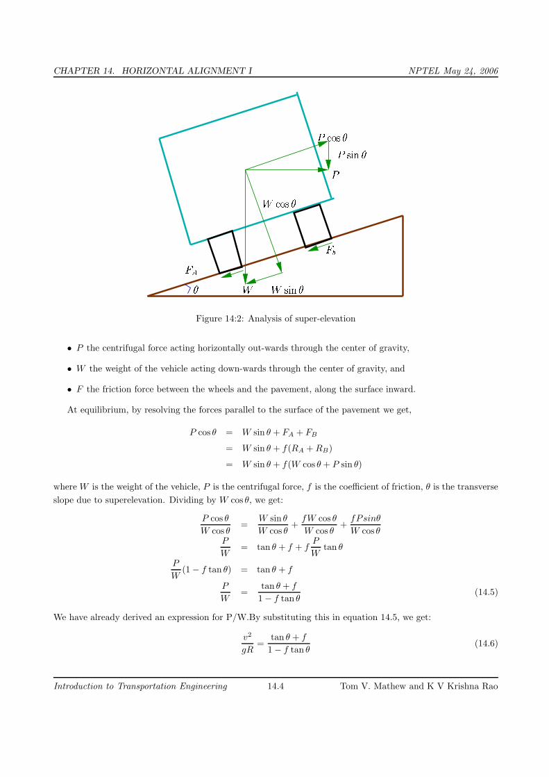
shown in figure 14:2 Forces acting on a vehicle on horizontal curve of radius R m at a speed of v m/sec2 are:
Introduction to Transportation Engineering 14.3 Tom V. Mathew and K V Krishna Rao
CHAPTER 14. HORIZONTAL ALIGNMENT I NPTEL May 24, 2006
� ���������
�
� �������
� �������
� �������
�
�
��
Figure 14:2: Analysis of super-elevation
• P the centrifugal force acting horizontally out-wards through the center of gravity,
• W the weight of the vehicle acting down-wards through the center of gravity, and
• F the friction force between the wheels and the pavement, along the surface inward.
At equilibrium, by resolving the forces parallel to the surface of the pavement we get,
P cos θ = W sin θ + FA + FB
= W sin θ + f(RA + RB)
= W sin θ + f(W cos θ + P sin θ)
where W is the weight of the vehicle, P is the centrifugal force, f is the coefficient of friction, θ is the transverse
slope due to superelevation. Dividing by W cos θ, we get:
P cos θ
W cos θ=
W sin θ
W cos θ+
fW cos θ
W cos θ+
fPsinθ
W cos θP
W= tan θ + f + f
P
Wtan θ
P
W(1 − f tan θ) = tan θ + f
P
W=
tan θ + f
1 − f tan θ(14.5)
We have already derived an expression for P/W.By substituting this in equation 14.5, we get:
v2
gR=
tan θ + f
1 − f tan θ(14.6)
Introduction to Transportation Engineering 14.4 Tom V. Mathew and K V Krishna Rao
CHAPTER 14. HORIZONTAL ALIGNMENT I NPTEL May 24, 2006
This is an exact expression for superelevation. But normally, f = 0.15 and θ < 4o, 1− f tan θ ≈ 1 and for small
θ, tan θ ≈ sin θ = E/B = e, then equation 14.6 becomes:
e + f =v2
gR(14.7)
where, e is the rate of super elevation, f the coefficient of lateral friction 0.15, v the speed of the vehicle in
m/sec2, R the radius of the curve in m and g = 9.8m/sec2.
Three specific cases that can arise from equation 14.7 are as follows:
1 If there is no friction due to some practical reasons, then f = 0 and equation 14.7 becomes e = v2
gR. This
results in the situation where the pressure on the outer and inner wheels are same; requiring very high
super-elevation e.
2 If there is no super-elevation provided due to some practical reasons, then e = 0 and equation 14.7 becomes
f = v2
gR. This results in a very high coefficient of friction.
3 If e = 0 and f = 0.15 then for safe traveling speed from equation 14.7 is given by vb =√
fgR where vb is
the restricted speed.
14.5 Summary
Design speed plays a major role in designing the elements of horizontal alignment. The most important element is
superelevation which is influenced by speed, radius of curve and frictional resistance of pavement. Superelevation
is necessary to balance centrifugal force. The design part is dealt in the next chapter.
14.6 Problems
1. The design speed recommended by IRC for National highways passign through rolling terrain is in the
range of
(a) 100-80
(b) 80-65
(c) 120-100
(d) 50-40
2. For safety against skidding, the condition to be satisfied is
(a) f¿ v2
gR
(b) f¡ v2
gR
(c) f¿ v
gR
(d) f= v2
gR
Introduction to Transportation Engineering 14.5 Tom V. Mathew and K V Krishna Rao
CHAPTER 14. HORIZONTAL ALIGNMENT I NPTEL May 24, 2006
14.7 Solutions
1. The design speed recommended by IRC for National highways passign through rolling terrain is in the
range of
(a) 100-80
(b) 80-65√
(c) 120-100
(d) 50-40
2. For safety against skidding, the condition to be satisfied is
(a) f¿ v2
gR
√
(b) f¡ v2
gR
(c) f¿ v
gR
(d) f= v2
gR
Introduction to Transportation Engineering 14.6 Tom V. Mathew and K V Krishna Rao
CHAPTER 15. HORIZONTAL ALIGNMENT II NPTEL May 24, 2006
Chapter 15
Horizontal alignment II
15.1 Overview
This section discusses the design of superelevation and how it is attained. A brief discussion about pavement
widening at curves is also given.
15.2 Guidelines on superelevation
While designing the various elements of the road like superelevation, we design it for a particular vehicle called
design vehicle which has some standard weight and dimensions. But in the actual case, the road has to cater
for mixed traffic. Different vehicles with different dimensions and varying speeds ply on the road. For example,
in the case of a heavily loaded truck with high centre of gravity and low speed, superelevation should be less,
otherwise chances of toppling are more. Taking into practical considerations of all such situations, IRC has
given some guidelines about the maximum and minimum superelevation etc. These are all discussed in detail
in the following sections.
15.2.1 Design of super-elevation
For fast moving vehicles, providing higher superelevation without considering coefficient of friction is safe, i.e.
centrifugal force is fully counteracted by the weight of the vehicle or superelevation. For slow moving vehicles,
providing lower superelevation considering coefficient of friction is safe, i.e.centrifugal force is counteracted by
superelevation and coefficient of friction . IRC suggests following design procedure:
Step 1 Find e for 75 percent of design speed, neglecting f , i.e e1 = (0.75v)2
gR.
Step 2 If e1 ≤ 0.07, then e = e1 = (0.75v)2
gR, else if e1 > 0.07 go to step 3.
Step 3 Find f1 for the design speed and max e, i.e f1 = v2
gR− e = v
2
gR− 0.07. If f1 < 0.15, then the maximum
e = 0.07 is safe for the design speed, else go to step 4.
Step 4 Find the allowable speed va for the maximum e = 0.07 and f = 0.15, va =√
0.22gR If va ≥ v then the
design is adequate, otherwise use speed adopt control measures or look for speed control measures.
Introduction to Transportation Engineering 15.1 Tom V. Mathew and K V Krishna Rao
CHAPTER 15. HORIZONTAL ALIGNMENT II NPTEL May 24, 2006
15.2.2 Maximum and minimum super-elevation
Depends on (a) slow moving vehicle and (b) heavy loaded trucks with high CG. IRC specifies a maximum
super-elevation of 7 percent for plain and rolling terrain, while that of hilly terrain is 10 percent and urban
road is 4 percent. The minimum super elevation is 2-4 percent for drainage purpose, especially for large
radius of the horizontal curve.
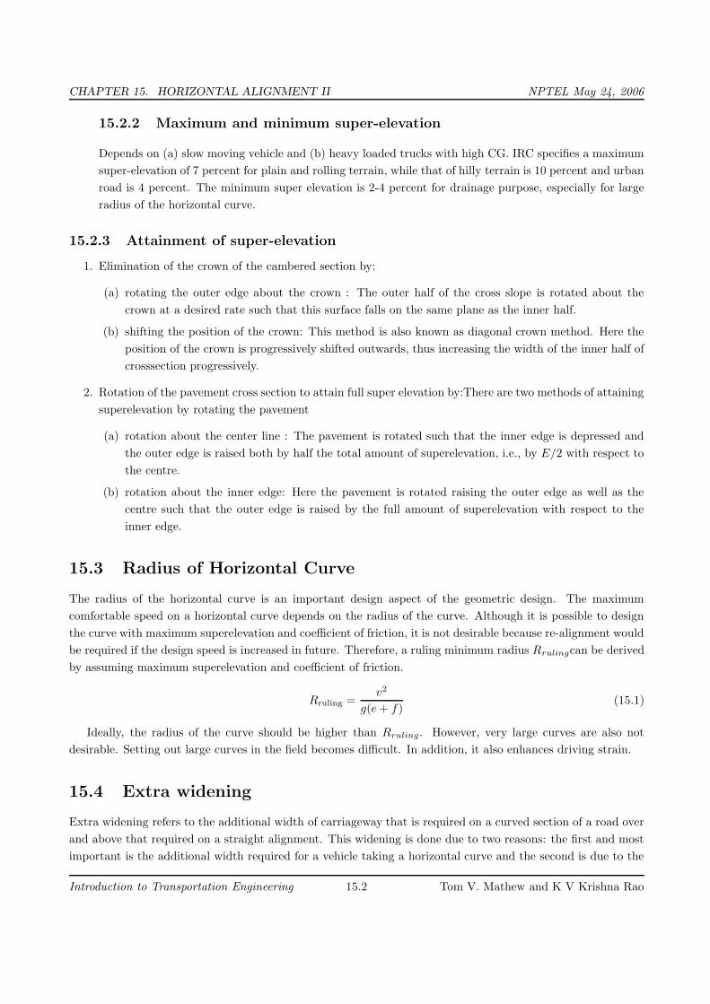
15.2.3 Attainment of super-elevation
1. Elimination of the crown of the cambered section by:
(a) rotating the outer edge about the crown : The outer half of the cross slope is rotated about the
crown at a desired rate such that this surface falls on the same plane as the inner half.
(b) shifting the position of the crown: This method is also known as diagonal crown method. Here the
position of the crown is progressively shifted outwards, thus increasing the width of the inner half of
crosssection progressively.
2. Rotation of the pavement cross section to attain full super elevation by:There are two methods of attaining
superelevation by rotating the pavement
(a) rotation about the center line : The pavement is rotated such that the inner edge is depressed and
the outer edge is raised both by half the total amount of superelevation, i.e., by E/2 with respect to
the centre.
(b) rotation about the inner edge: Here the pavement is rotated raising the outer edge as well as the
centre such that the outer edge is raised by the full amount of superelevation with respect to the
inner edge.
15.3 Radius of Horizontal Curve
The radius of the horizontal curve is an important design aspect of the geometric design. The maximum
comfortable speed on a horizontal curve depends on the radius of the curve. Although it is possible to design
the curve with maximum superelevation and coefficient of friction, it is not desirable because re-alignment would
be required if the design speed is increased in future. Therefore, a ruling minimum radius Rrulingcan be derived
by assuming maximum superelevation and coefficient of friction.
Rruling =v2
g(e + f)(15.1)
Ideally, the radius of the curve should be higher than Rruling . However, very large curves are also not
desirable. Setting out large curves in the field becomes difficult. In addition, it also enhances driving strain.
15.4 Extra widening
Extra widening refers to the additional width of carriageway that is required on a curved section of a road over
and above that required on a straight alignment. This widening is done due to two reasons: the first and most
important is the additional width required for a vehicle taking a horizontal curve and the second is due to the
Introduction to Transportation Engineering 15.2 Tom V. Mathew and K V Krishna Rao
CHAPTER 15. HORIZONTAL ALIGNMENT II NPTEL May 24, 2006
tendency of the drivers to ply away from the edge of the carriageway as they drive on a curve. The first is
referred as the mechanical widening and the second is called the psychological widening. These are discussed
in detail below.
15.4.1 Mechanical widening
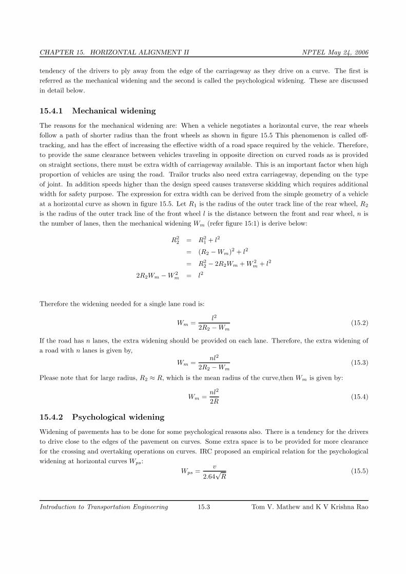
The reasons for the mechanical widening are: When a vehicle negotiates a horizontal curve, the rear wheels
follow a path of shorter radius than the front wheels as shown in figure 15.5 This phenomenon is called off-
tracking, and has the effect of increasing the effective width of a road space required by the vehicle. Therefore,
to provide the same clearance between vehicles traveling in opposite direction on curved roads as is provided
on straight sections, there must be extra width of carriageway available. This is an important factor when high
proportion of vehicles are using the road. Trailor trucks also need extra carriageway, depending on the type
of joint. In addition speeds higher than the design speed causes transverse skidding which requires additional
width for safety purpose. The expression for extra width can be derived from the simple geometry of a vehicle
at a horizontal curve as shown in figure 15.5. Let R1 is the radius of the outer track line of the rear wheel, R2
is the radius of the outer track line of the front wheel l is the distance between the front and rear wheel, n is
the number of lanes, then the mechanical widening Wm (refer figure 15:1) is derive below:
R2
2= R2
1+ l2
= (R2 − Wm)2 + l2
= R2
2− 2R2Wm + W 2
m + l2
2R2Wm − W 2
m= l2
Therefore the widening needed for a single lane road is:
Wm =l2
2R2 − Wm
(15.2)
If the road has n lanes, the extra widening should be provided on each lane. Therefore, the extra widening of
a road with n lanes is given by,
Wm =nl2
2R2 − Wm
(15.3)
Please note that for large radius, R2 ≈ R, which is the mean radius of the curve,then Wm is given by:
Wm =nl2
2R(15.4)
15.4.2 Psychological widening
Widening of pavements has to be done for some psychological reasons also. There is a tendency for the drivers
to drive close to the edges of the pavement on curves. Some extra space is to be provided for more clearance
for the crossing and overtaking operations on curves. IRC proposed an empirical relation for the psychological
widening at horizontal curves Wps:
Wps =v
2.64√
R(15.5)
Introduction to Transportation Engineering 15.3 Tom V. Mathew and K V Krishna Rao
CHAPTER 15. HORIZONTAL ALIGNMENT II NPTEL May 24, 2006
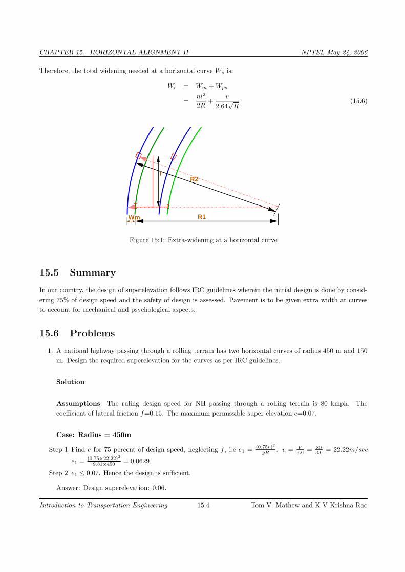
Therefore, the total widening needed at a horizontal curve We is:
We = Wm + Wps
=nl2
2R+
v
2.64√
R(15.6)
Wm R1
R2l
Figure 15:1: Extra-widening at a horizontal curve
15.5 Summary
In our country, the design of superelevation follows IRC guidelines wherein the initial design is done by consid-
ering 75% of design speed and the safety of design is assessed. Pavement is to be given extra width at curves
to account for mechanical and psychological aspects.
15.6 Problems
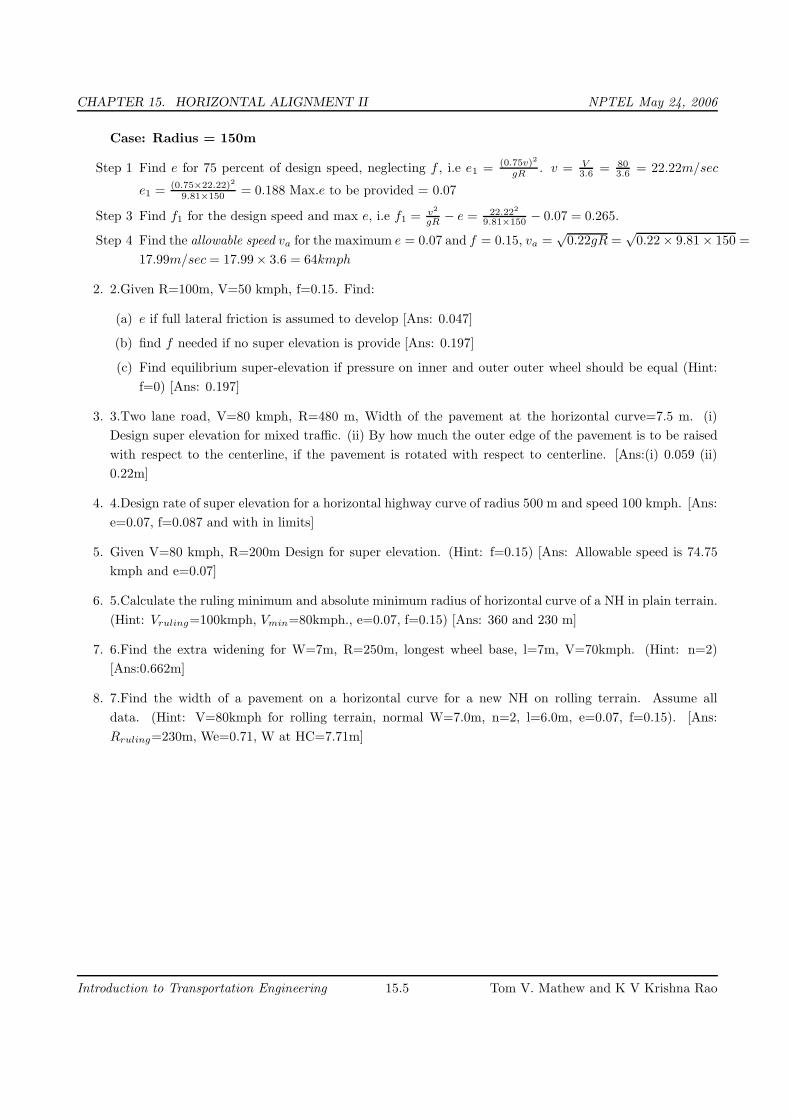
1. A national highway passing through a rolling terrain has two horizontal curves of radius 450 m and 150
m. Design the required superelevation for the curves as per IRC guidelines.
Solution
Assumptions The ruling design speed for NH passing through a rolling terrain is 80 kmph. The
coefficient of lateral friction f=0.15. The maximum permissible super elevation e=0.07.
Case: Radius = 450m
Step 1 Find e for 75 percent of design speed, neglecting f , i.e e1 = (0.75v)2
gR. v = V
3.6= 80
3.6= 22.22m/sec
e1 = (0.75×22.22)2
9.81×450= 0.0629
Step 2 e1 ≤ 0.07. Hence the design is sufficient.
Answer: Design superelevation: 0.06.
Introduction to Transportation Engineering 15.4 Tom V. Mathew and K V Krishna Rao
CHAPTER 15. HORIZONTAL ALIGNMENT II NPTEL May 24, 2006
Case: Radius = 150m
Step 1 Find e for 75 percent of design speed, neglecting f , i.e e1 = (0.75v)2
gR. v = V
3.6= 80
3.6= 22.22m/sec
e1 = (0.75×22.22)2
9.81×150= 0.188 Max.e to be provided = 0.07
Step 3 Find f1 for the design speed and max e, i.e f1 = v2
gR− e = 22.22
2
9.81×150− 0.07 = 0.265.
Step 4 Find the allowable speed va for the maximum e = 0.07 and f = 0.15, va =√
0.22gR =√
0.22× 9.81× 150 =
17.99m/sec = 17.99× 3.6 = 64kmph
2. 2.Given R=100m, V=50 kmph, f=0.15. Find:
(a) e if full lateral friction is assumed to develop [Ans: 0.047]
(b) find f needed if no super elevation is provide [Ans: 0.197]
(c) Find equilibrium super-elevation if pressure on inner and outer outer wheel should be equal (Hint:
f=0) [Ans: 0.197]
3. 3.Two lane road, V=80 kmph, R=480 m, Width of the pavement at the horizontal curve=7.5 m. (i)
Design super elevation for mixed traffic. (ii) By how much the outer edge of the pavement is to be raised
with respect to the centerline, if the pavement is rotated with respect to centerline. [Ans:(i) 0.059 (ii)
0.22m]
4. 4.Design rate of super elevation for a horizontal highway curve of radius 500 m and speed 100 kmph. [Ans:
e=0.07, f=0.087 and with in limits]
5. Given V=80 kmph, R=200m Design for super elevation. (Hint: f=0.15) [Ans: Allowable speed is 74.75
kmph and e=0.07]
6. 5.Calculate the ruling minimum and absolute minimum radius of horizontal curve of a NH in plain terrain.
(Hint: Vruling=100kmph, Vmin=80kmph., e=0.07, f=0.15) [Ans: 360 and 230 m]
7. 6.Find the extra widening for W=7m, R=250m, longest wheel base, l=7m, V=70kmph. (Hint: n=2)
[Ans:0.662m]
8. 7.Find the width of a pavement on a horizontal curve for a new NH on rolling terrain. Assume all
data. (Hint: V=80kmph for rolling terrain, normal W=7.0m, n=2, l=6.0m, e=0.07, f=0.15). [Ans:
Rruling=230m, We=0.71, W at HC=7.71m]
Introduction to Transportation Engineering 15.5 Tom V. Mathew and K V Krishna Rao
CHAPTER 16. HORIZONTAL ALIGNMENT III NPTEL May 24, 2006
Chapter 16
Horizontal alignment III
16.1 Overview
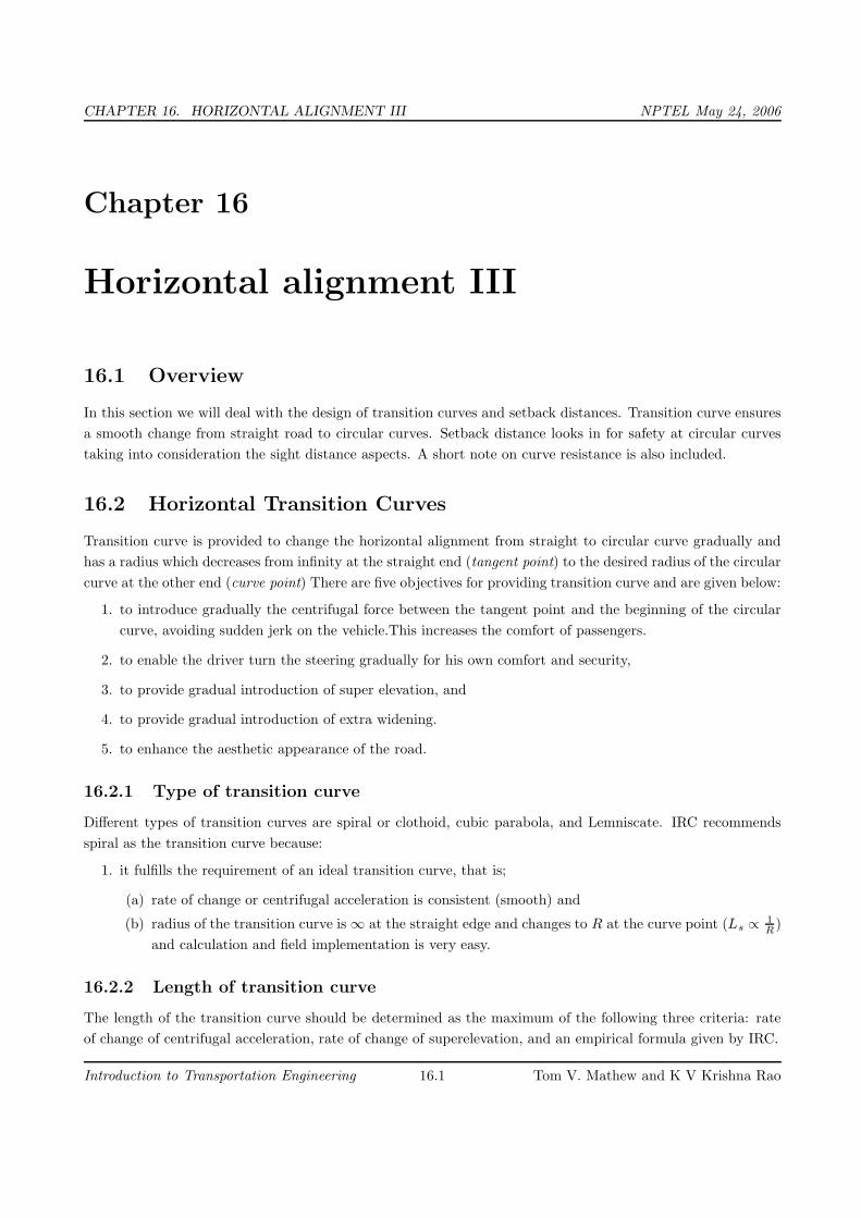
In this section we will deal with the design of transition curves and setback distances. Transition curve ensures
a smooth change from straight road to circular curves. Setback distance looks in for safety at circular curves
taking into consideration the sight distance aspects. A short note on curve resistance is also included.
16.2 Horizontal Transition Curves
Transition curve is provided to change the horizontal alignment from straight to circular curve gradually and
has a radius which decreases from infinity at the straight end (tangent point) to the desired radius of the circular
curve at the other end (curve point) There are five objectives for providing transition curve and are given below:
1. to introduce gradually the centrifugal force between the tangent point and the beginning of the circular
curve, avoiding sudden jerk on the vehicle.This increases the comfort of passengers.
2. to enable the driver turn the steering gradually for his own comfort and security,
3. to provide gradual introduction of super elevation, and
4. to provide gradual introduction of extra widening.
5. to enhance the aesthetic appearance of the road.
16.2.1 Type of transition curve
Different types of transition curves are spiral or clothoid, cubic parabola, and Lemniscate. IRC recommends
spiral as the transition curve because:
1. it fulfills the requirement of an ideal transition curve, that is;
(a) rate of change or centrifugal acceleration is consistent (smooth) and
(b) radius of the transition curve is ∞ at the straight edge and changes to R at the curve point (Ls ∝ 1
R)
and calculation and field implementation is very easy.
16.2.2 Length of transition curve
The length of the transition curve should be determined as the maximum of the following three criteria: rate
of change of centrifugal acceleration, rate of change of superelevation, and an empirical formula given by IRC.
Introduction to Transportation Engineering 16.1 Tom V. Mathew and K V Krishna Rao
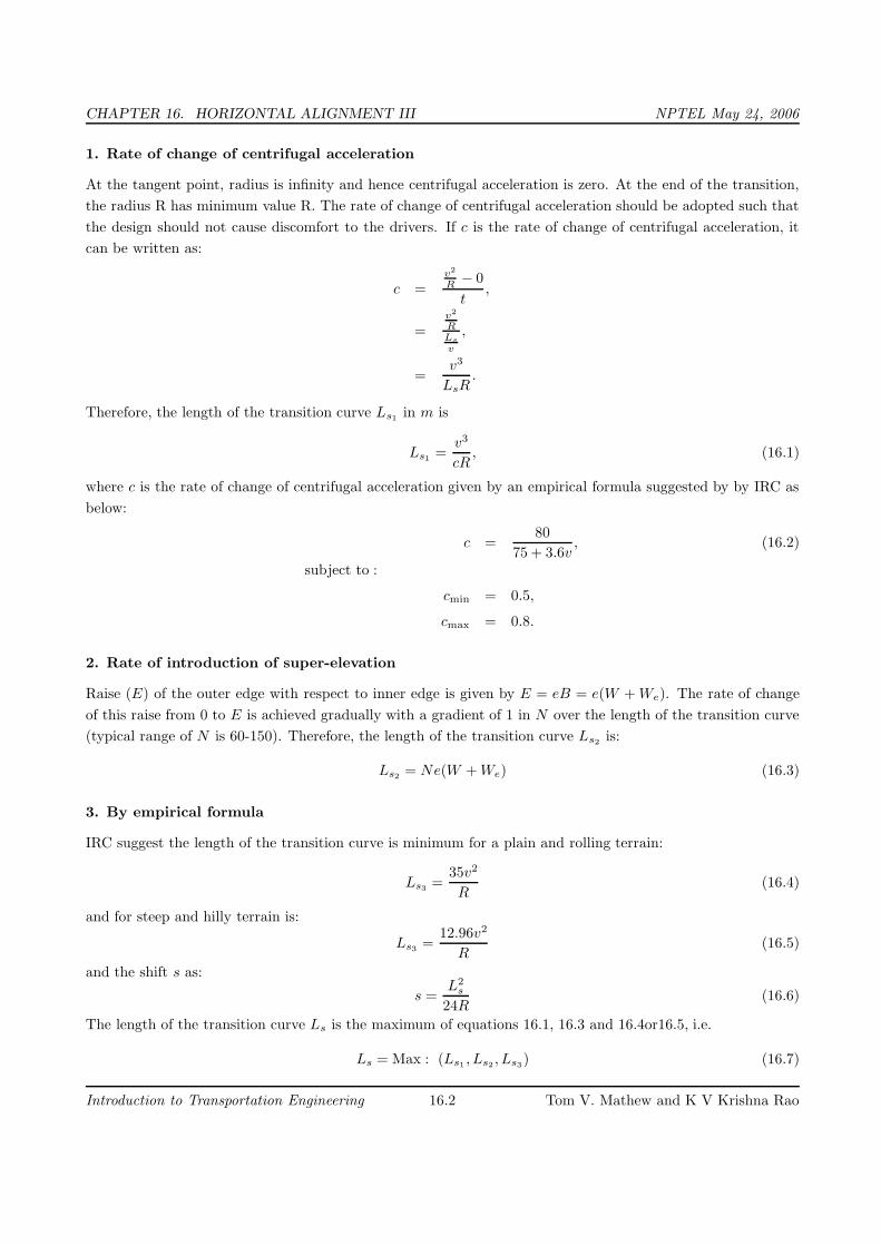
CHAPTER 16. HORIZONTAL ALIGNMENT III NPTEL May 24, 2006
1. Rate of change of centrifugal acceleration
At the tangent point, radius is infinity and hence centrifugal acceleration is zero. At the end of the transition,
the radius R has minimum value R. The rate of change of centrifugal acceleration should be adopted such that
the design should not cause discomfort to the drivers. If c is the rate of change of centrifugal acceleration, it
can be written as:
c =v2
R− 0
t,
=v2
R
Ls
v
,
=v3
LsR.
Therefore, the length of the transition curve Ls1in m is
Ls1=
v3
cR, (16.1)
where c is the rate of change of centrifugal acceleration given by an empirical formula suggested by by IRC as
below:
c =80
75 + 3.6v, (16.2)
subject to :
cmin = 0.5,
cmax = 0.8.
2. Rate of introduction of super-elevation
Raise (E) of the outer edge with respect to inner edge is given by E = eB = e(W + We). The rate of change
of this raise from 0 to E is achieved gradually with a gradient of 1 in N over the length of the transition curve
(typical range of N is 60-150). Therefore, the length of the transition curve Ls2is:
Ls2= Ne(W + We) (16.3)
3. By empirical formula
IRC suggest the length of the transition curve is minimum for a plain and rolling terrain:
Ls3=
35v2
R(16.4)
and for steep and hilly terrain is:
Ls3=
12.96v2
R(16.5)
and the shift s as:
s =L2
s
24R(16.6)
The length of the transition curve Ls is the maximum of equations 16.1, 16.3 and 16.4or16.5, i.e.
Ls = Max : (Ls1, Ls2
, Ls3) (16.7)
Introduction to Transportation Engineering 16.2 Tom V. Mathew and K V Krishna Rao
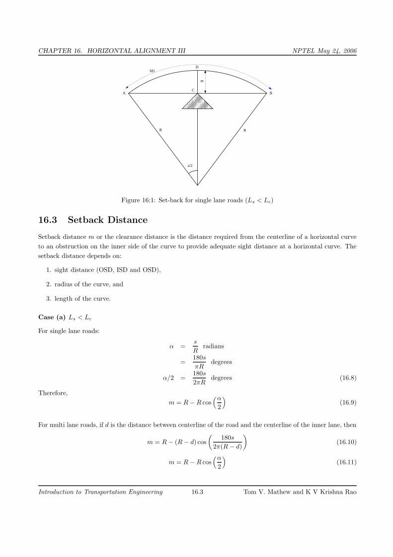
CHAPTER 16. HORIZONTAL ALIGNMENT III NPTEL May 24, 2006
���������������������������������������������������������������������������������������������������������������������������������������������������������������������������������������������������������������������������������������
�����������������������������������������������������������������������������������������������������������������������������������������������������������������������������������������������������������������
m
R
a/2
R
D
A B
SD
C
Figure 16:1: Set-back for single lane roads (Ls < Lc)
16.3 Setback Distance
Setback distance m or the clearance distance is the distance required from the centerline of a horizontal curve
to an obstruction on the inner side of the curve to provide adequate sight distance at a horizontal curve. The
setback distance depends on:
1. sight distance (OSD, ISD and OSD),
2. radius of the curve, and
3. length of the curve.
Case (a) Ls < Lc
For single lane roads:
α =s
Rradians
=180s
πRdegrees
α/2 =180s
2πRdegrees (16.8)
Therefore,
m = R − R cos(α
2
)
(16.9)
For multi lane roads, if d is the distance between centerline of the road and the centerline of the inner lane, then
m = R − (R − d) cos
(
180s
2π(R − d)
)
(16.10)
m = R − R cos(α
2
)
(16.11)
Introduction to Transportation Engineering 16.3 Tom V. Mathew and K V Krishna Rao
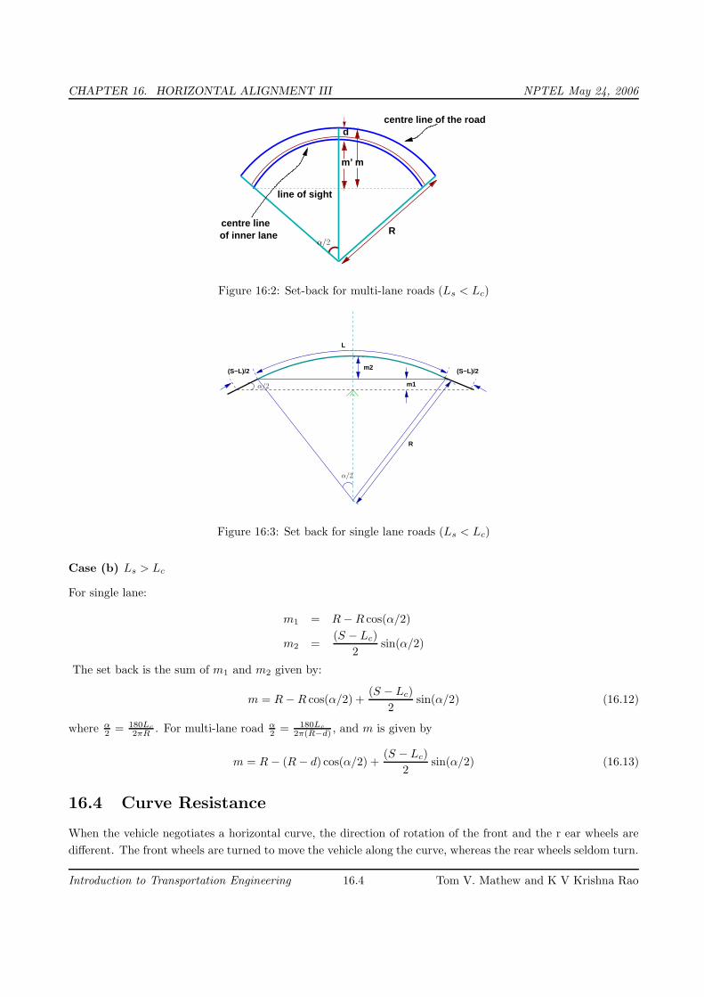
CHAPTER 16. HORIZONTAL ALIGNMENT III NPTEL May 24, 2006
m’ m
d
line of sight
R
centre line of the road
centre line of inner lane
α/2
Figure 16:2: Set-back for multi-lane roads (Ls < Lc)
(S−L)/2
L
(S−L)/2
m1
m2
R
α/2
α/2
Figure 16:3: Set back for single lane roads (Ls < Lc)
Case (b) Ls > Lc
For single lane:
m1 = R − R cos(α/2)
m2 =(S − Lc)
2sin(α/2)
The set back is the sum of m1 and m2 given by:
m = R − R cos(α/2) +(S − Lc)
2sin(α/2) (16.12)
where α
2= 180Lc
2πR. For multi-lane road α
2= 180Lc
2π(R−d), and m is given by
m = R − (R − d) cos(α/2) +(S − Lc)
2sin(α/2) (16.13)
16.4 Curve Resistance
When the vehicle negotiates a horizontal curve, the direction of rotation of the front and the r ear wheels are
different. The front wheels are turned to move the vehicle along the curve, whereas the rear wheels seldom turn.
Introduction to Transportation Engineering 16.4 Tom V. Mathew and K V Krishna Rao
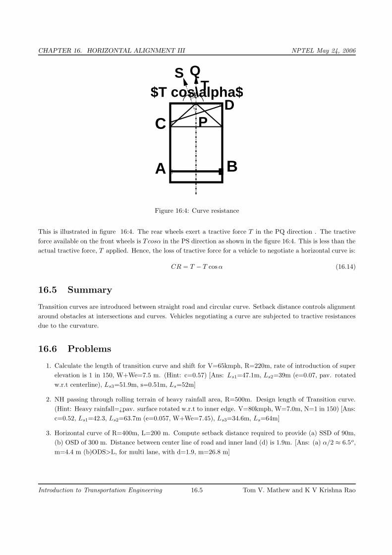
CHAPTER 16. HORIZONTAL ALIGNMENT III NPTEL May 24, 2006
PD
TS Q
A B
C
$T cos\alpha$α
Figure 16:4: Curve resistance
This is illustrated in figure 16:4. The rear wheels exert a tractive force T in the PQ direction . The tractive
force available on the front wheels is Tcosα in the PS direction as shown in the figure 16:4. This is less than the
actual tractive force, T applied. Hence, the loss of tractive force for a vehicle to negotiate a horizontal curve is:
CR = T − T cosα (16.14)
16.5 Summary
Transition curves are introduced between straight road and circular curve. Setback distance controls alignment
around obstacles at intersections and curves. Vehicles negotiating a curve are subjected to tractive resistances
due to the curvature.
16.6 Problems
1. Calculate the length of transition curve and shift for V=65kmph, R=220m, rate of introduction of super
elevation is 1 in 150, W+We=7.5 m. (Hint: c=0.57) [Ans: Ls1=47.1m, Ls2=39m (e=0.07, pav. rotated
w.r.t centerline), Ls3=51.9m, s=0.51m, Ls=52m]
2. NH passing through rolling terrain of heavy rainfall area, R=500m. Design length of Transition curve.
(Hint: Heavy rainfall=¿pav. surface rotated w.r.t to inner edge. V=80kmph, W=7.0m, N=1 in 150) [Ans:
c=0.52, Ls1=42.3, Ls2=63.7m (e=0.057, W+We=7.45), Ls3=34.6m, Ls=64m]
3. Horizontal curve of R=400m, L=200 m. Compute setback distance required to provide (a) SSD of 90m,
(b) OSD of 300 m. Distance between center line of road and inner land (d) is 1.9m. [Ans: (a) α/2 ≈ 6.5o,
m=4.4 m (b)ODS>L, for multi lane, with d=1.9, m=26.8 m]
Introduction to Transportation Engineering 16.5 Tom V. Mathew and K V Krishna Rao
CHAPTER 17. VERTICAL ALIGNMENT-I NPTEL May 24, 2006
Chapter 17
Vertical alignment-I
17.1 Overview
The vertical alignment of a road consists of gradients(straight lines in a vertical plane) and vertical curves.
The vertical alignment is usually drawn as a profile, which is a graph with elevation as vertical axis and the
horizontal distance along the centre line of the road as the the horizontal axis. Just as a circular curve is used
to connect horizontal straight stretches of road, vertical curves connect two gradients. When these two curves
meet, they form either convex or concave. The former is called a summit curve, while the latter is called a
valley curve. This section covers a discussion on gradient and summit curves.
17.2 Gradient
Gradient is the rate of rise or fall along the length of the road with respect to the horizontal. While aligning a
highway, the gradient is decided designing the vertical curve. Before finalizing the gradients, the construction
cost, vehicular operation cost and the practical problems in the site also has to be considered. Usually steep
gradients are avoided as far as possible because of the difficulty to climb and increase in the construction cost.
More about gradients are discussed below.
17.2.1 Effect of gradient
The effect of long steep gradient on the vehicular speed is considerable. This is particularly important in roads
where the proportion of heavy vehicles is significant. Due to restrictive sight distance at uphill gradients the
speed of traffic is often controlled by these heavy vehicles. As a result, not only the operating costs of the vehicles
are increased, but also capacity of the roads will have to be reduced. Further, due to high differential speed
between heavy and light vehicles, and between uphill and downhill gradients, accidents abound in gradients.
17.2.2 Representation of gradient
The positive gradient or the ascending gradient is denoted as +n and the negative gradient as −n. The deviation
angle N is: when two grades meet, the angle which measures the change of direction and is given by the algebraic
difference between the two grades (n1 − (−n2)) = n1 + n2 = α1 + α2. Example: 1 in 30 = 3.33% ≈ 2o is
a steep gradient, while 1 in 50 = 2% ≈ 1o10′
is a flatter gradient. The gradient representation is illustrated in
the figure 17:1.
Introduction to Transportation Engineering 17.1 Tom V. Mathew and K V Krishna Rao
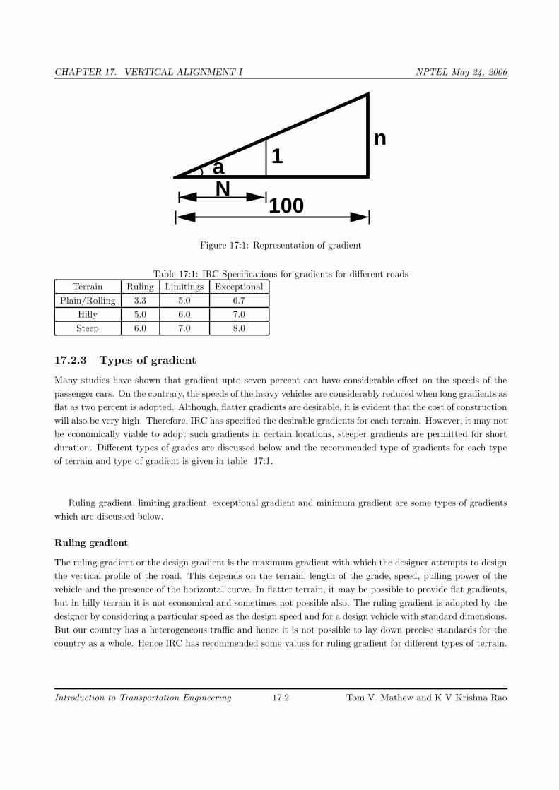
CHAPTER 17. VERTICAL ALIGNMENT-I NPTEL May 24, 2006
1n
100
aN
Figure 17:1: Representation of gradient
Table 17:1: IRC Specifications for gradients for different roads
Terrain Ruling Limitings Exceptional
Plain/Rolling 3.3 5.0 6.7
Hilly 5.0 6.0 7.0
Steep 6.0 7.0 8.0
17.2.3 Types of gradient
Many studies have shown that gradient upto seven percent can have considerable effect on the speeds of the
passenger cars. On the contrary, the speeds of the heavy vehicles are considerably reduced when long gradients as
flat as two percent is adopted. Although, flatter gradients are desirable, it is evident that the cost of construction
will also be very high. Therefore, IRC has specified the desirable gradients for each terrain. However, it may not
be economically viable to adopt such gradients in certain locations, steeper gradients are permitted for short
duration. Different types of grades are discussed below and the recommended type of gradients for each type
of terrain and type of gradient is given in table 17:1.
Ruling gradient, limiting gradient, exceptional gradient and minimum gradient are some types of gradients
which are discussed below.
Ruling gradient
The ruling gradient or the design gradient is the maximum gradient with which the designer attempts to design
the vertical profile of the road. This depends on the terrain, length of the grade, speed, pulling power of the
vehicle and the presence of the horizontal curve. In flatter terrain, it may be possible to provide flat gradients,
but in hilly terrain it is not economical and sometimes not possible also. The ruling gradient is adopted by the
designer by considering a particular speed as the design speed and for a design vehicle with standard dimensions.
But our country has a heterogeneous traffic and hence it is not possible to lay down precise standards for the
country as a whole. Hence IRC has recommended some values for ruling gradient for different types of terrain.
Introduction to Transportation Engineering 17.2 Tom V. Mathew and K V Krishna Rao
CHAPTER 17. VERTICAL ALIGNMENT-I NPTEL May 24, 2006
Limiting gradient
This gradient is adopted when the ruling gradient results in enormous increase in cost of construction. On
rolling terrain and hilly terrain it may be frequently necessary to adopt limiting gradient. But the length of the
limiting gradient stretches should be limited and must be sandwiched by either straight roads or easier grades.
Exceptional gradient
Exceptional gradient are very steeper gradients given at unavoidable situations. They should be limited for
short stretches not exceeding about 100 metres at a stretch. In mountainous and steep terrain, successive
exceptional gradients must be separated by a minimum 100 metre length gentler gradient. At hairpin bends,
the gradient is restricted to 2.5%.
Critical length of the grade
The maximum length of the ascending gradient which a loaded truck can operate without undue reduction in
speed is called critical length of the grade. A speed of 25 kmph is a reasonable value. This value depends on
the size, power, load, grad-ability of the truck, initial speed, final desirable minimum speed etc.
Minimum gradient
This is important only at locations where surface drainage is important. Camber will take care of the lateral
drainage. But the longitudinal drainage along the side drains require some slope for smooth flow of water.
Therefore minimum gradient is provided for drainage purpose and it depends on the rain fall, type of soil and
other site conditions. A minimum of 1 in 500 may be sufficient for concrete drain and 1 in 200 for open soil
drains are found to give satisfactory performance..
17.2.4 Creeper lane
When the uphill climb is extremely long, it may be desirable to introduce an additional lane so as to allow
slow ascending vehicles to be removed from the main stream so that the fast moving vehicles are not affected.
Such a newly introduced lane is called creeper lane. There are no hard and fast rules as when to introduce a
creeper lane. But generally, it can be said that it is desirable to provide a creeper lane when the speed of the
vehicle gets reduced to half the design speed. When there is no restrictive sight distance to reduce the speed
of the approaching vehicle, the additional lane may be initiated at some distance uphill from the beginning of
the slope. But when the restrictions are responsible for the lowering of speeds, obviously the lane should be
initiated at a point closer to the bottom of the hill. Also the creeper lane should end at a point well beyond the
hill crest, so that the slow moving vehicles can return back to the normal lane without any danger. In addition,
the creeper lane should not end suddenly, but only in a tapered manner for efficient as well as safer transition
of vehicles to the normal lane.
17.2.5 Grade compensation
While a vehicle is negotiating a horizontal curve, if there is a gradient also, then there will be increased resistance
to traction due to both curve and the gradient. In such cases, the total resistance should not exceed the resistance
due to gradient specified. For the design, in some cases this maximum value is limited to the ruling gradient
Introduction to Transportation Engineering 17.3 Tom V. Mathew and K V Krishna Rao
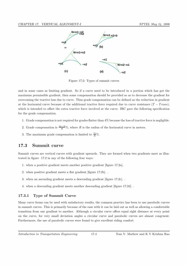
CHAPTER 17. VERTICAL ALIGNMENT-I NPTEL May 24, 2006
(a)
(c) (d)
−n2
N=n1+n2
+n1
+n1
N=n1−n2+n2
+n1 (b)
−n1
N=n2−n1
−n2
N=n1 n2=0
Figure 17:2: Types of summit curves
and in some cases as limiting gradient. So if a curve need to be introduced in a portion which has got the
maximum permissible gradient, then some compensation should be provided so as to decrease the gradient for
overcoming the tractive loss due to curve. Thus grade compensation can be defined as the reduction in gradient
at the horizontal curve because of the additional tractive force required due to curve resistance (T − Tcosα),
which is intended to offset the extra tractive force involved at the curve. IRC gave the following specification
for the grade compensation.
1. Grade compensation is not required for grades flatter than 4% because the loss of tractive force is negligible.
2. Grade compensation is 30+R
R%, where R is the radius of the horizontal curve in meters.
3. The maximum grade compensation is limited to 75
R%.
17.3 Summit curve
Summit curves are vertical curves with gradient upwards. They are formed when two gradients meet as illus-
trated in figure 17:2 in any of the following four ways:
1. when a positive gradient meets another positive gradient [figure 17:2a].
2. when positive gradient meets a flat gradient [figure 17:2b]. .
3. when an ascending gradient meets a descending gradient [figure 17:2c]. .
4. when a descending gradient meets another descending gradient [figure 17:2d]. .
17.3.1 Type of Summit Curve
Many curve forms can be used with satisfactory results, the common practice has been to use parabolic curves
in summit curves. This is primarily because of the ease with it can be laid out as well as allowing a comfortable
transition from one gradient to another. Although a circular curve offers equal sight distance at every point
on the curve, for very small deviation angles a circular curve and parabolic curves are almost congruent.
Furthermore, the use of parabolic curves were found to give excellent riding comfort.
Introduction to Transportation Engineering 17.4 Tom V. Mathew and K V Krishna Rao
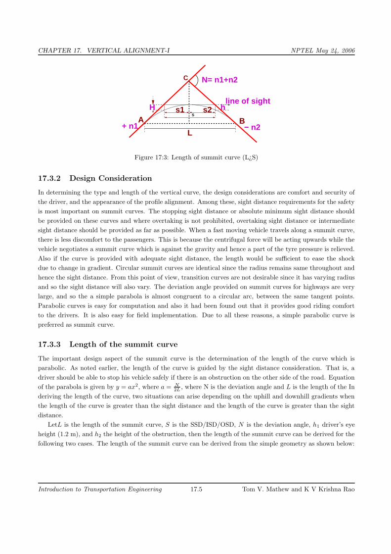
CHAPTER 17. VERTICAL ALIGNMENT-I NPTEL May 24, 2006
S
N= n1+n2
line of sight
− n2B
+ n1A
s1 s2 hH
C
L
Figure 17:3: Length of summit curve (L¿S)
17.3.2 Design Consideration
In determining the type and length of the vertical curve, the design considerations are comfort and security of
the driver, and the appearance of the profile alignment. Among these, sight distance requirements for the safety
is most important on summit curves. The stopping sight distance or absolute minimum sight distance should
be provided on these curves and where overtaking is not prohibited, overtaking sight distance or intermediate
sight distance should be provided as far as possible. When a fast moving vehicle travels along a summit curve,
there is less discomfort to the passengers. This is because the centrifugal force will be acting upwards while the
vehicle negotiates a summit curve which is against the gravity and hence a part of the tyre pressure is relieved.
Also if the curve is provided with adequate sight distance, the length would be sufficient to ease the shock
due to change in gradient. Circular summit curves are identical since the radius remains same throughout and
hence the sight distance. From this point of view, transition curves are not desirable since it has varying radius
and so the sight distance will also vary. The deviation angle provided on summit curves for highways are very
large, and so the a simple parabola is almost congruent to a circular arc, between the same tangent points.
Parabolic curves is easy for computation and also it had been found out that it provides good riding comfort
to the drivers. It is also easy for field implementation. Due to all these reasons, a simple parabolic curve is
preferred as summit curve.
17.3.3 Length of the summit curve
The important design aspect of the summit curve is the determination of the length of the curve which is
parabolic. As noted earlier, the length of the curve is guided by the sight distance consideration. That is, a
driver should be able to stop his vehicle safely if there is an obstruction on the other side of the road. Equation
of the parabola is given by y = ax2, where a = N
2L, where N is the deviation angle and L is the length of the In
deriving the length of the curve, two situations can arise depending on the uphill and downhill gradients when
the length of the curve is greater than the sight distance and the length of the curve is greater than the sight
distance.
LetL is the length of the summit curve, S is the SSD/ISD/OSD, N is the deviation angle, h1 driver’s eye
height (1.2 m), and h2 the height of the obstruction, then the length of the summit curve can be derived for the
following two cases. The length of the summit curve can be derived from the simple geometry as shown below:
Introduction to Transportation Engineering 17.5 Tom V. Mathew and K V Krishna Rao
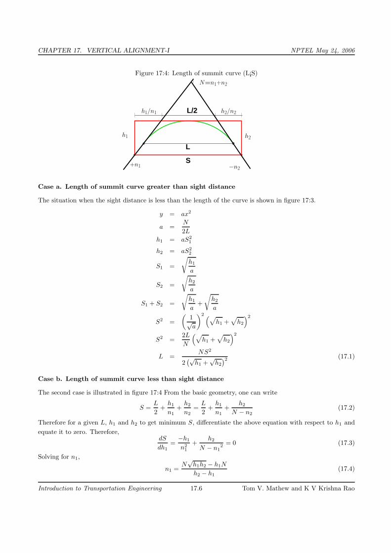
CHAPTER 17. VERTICAL ALIGNMENT-I NPTEL May 24, 2006
Figure 17:4: Length of summit curve (L¡S)
L/2
L
S+n1
h1/n1
h2
−n2
h1
h2/n2
N=n1+n2
Case a. Length of summit curve greater than sight distance
The situation when the sight distance is less than the length of the curve is shown in figure 17:3.
y = ax2
a =N
2L
h1 = aS2
1
h2 = aS2
2
S1 =
√
h1
a
S2 =
√
h2
a
S1 + S2 =
√
h1
a+
√
h2
a
S2 =
(
1√
a
)2(
√
h1 +√
h2
)2
S2 =2L
N
(
√
h1 +√
h2
)2
L =NS2
2(√
h1 +√
h2
)2(17.1)
Case b. Length of summit curve less than sight distance
The second case is illustrated in figure 17:4 From the basic geometry, one can write
S =L
2+
h1
n1
+h2
n2
=L
2+
h1
n1
+h2
N − n2
(17.2)
Therefore for a given L, h1 and h2 to get minimum S, differentiate the above equation with respect to h1 and
equate it to zero. Therefore,dS
dh1
=−h1
n2
1
+h2
N − n12
= 0 (17.3)
Solving for n1,
n1 =N√
h1h2 − h1N
h2 − h1
(17.4)
Introduction to Transportation Engineering 17.6 Tom V. Mathew and K V Krishna Rao
CHAPTER 17. VERTICAL ALIGNMENT-I NPTEL May 24, 2006
Now we can substitute n back to get the value of minimum value of L for a given n1, n2, h1 and h2. Therefore,
S =L
2+
h1
N√
h1h2−h1N
h2−h1
+h2
N − N√
h1h2−h1N
h2−h1
(17.5)
Solving for L,
L = 2S −
(√2h1 +
√2h2
)2
N(17.6)
When stopping sight distance is considered the height of driver’s eye above the road surface (h1) is taken as
1.2 metres, and height of object above the pavement surface (h2) is taken as 0.15 metres. If overtaking sight
distance is considered, then the value of driver’s eye height (h1) and the height of the obstruction (h2) are taken
equal as 1.2 metres.
17.4 Summary
Different types of gradients and IRC recommendations for their maximum and minimum limit were discussed.
At points of combination of horizontal curve and gradient, grade compensation has to be provided. Due to
changes in grade in the vertical alignment of the highway, vertical curves become essential. Summit curve,
which is a type of vertical curve was discussed in detail in the chapter. One of the application of summit curves
that can be seen usually in the urban areas are where fly-overs come.
17.5 Problems
1. A vertical summit curve is formed by n1 = +3.0% and n2 = −5.0%. Design the length of the summit
curve for V=80 kmph. (Hint: SSD=128m). [Ans: 298m]
2. n1 ==1 in 1–, n2 = 1 in 120. Design summit curve for V=80kmph, OSD=470m. [Ans: L=417m]
3. n1 = +1/50 and n2 = −1/80, SSD=180m, OSD=640m. Due to site constraints, L is limited to 500m.
Calculate the length of summit curve to meet SSD, ISD and OSD. Discuss results. [Ans: L for SSD=240m,
okay, L for OSD=1387m, > 500m not okay, L for ISD=439m okay.]
Introduction to Transportation Engineering 17.7 Tom V. Mathew and K V Krishna Rao
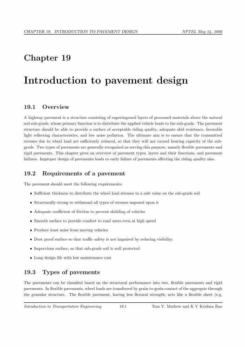
CHAPTER 19. INTRODUCTION TO PAVEMENT DESIGN NPTEL May 24, 2006
Chapter 19
Introduction to pavement design
19.1 Overview
A highway pavement is a structure consisting of superimposed layers of processed materials above the natural
soil sub-grade, whose primary function is to distribute the applied vehicle loads to the sub-grade. The pavement
structure should be able to provide a surface of acceptable riding quality, adequate skid resistance, favorable
light reflecting characteristics, and low noise pollution. The ultimate aim is to ensure that the transmitted
stresses due to wheel load are sufficiently reduced, so that they will not exceed bearing capacity of the sub-
grade. Two types of pavements are generally recognized as serving this purpose, namely flexible pavements and
rigid pavements. This chapter gives an overview of pavement types, layers and their functions, and pavement
failures. Improper design of pavements leads to early failure of pavements affecting the riding quality also.
19.2 Requirements of a pavement
The pavement should meet the following requirements:
• Sufficient thickness to distribute the wheel load stresses to a safe value on the sub-grade soil
• Structurally strong to withstand all types of stresses imposed upon it
• Adequate coefficient of friction to prevent skidding of vehicles
• Smooth surface to provide comfort to road users even at high speed
• Produce least noise from moving vehicles
• Dust proof surface so that traffic safety is not impaired by reducing visibility.
• Impervious surface, so that sub-grade soil is well protected
• Long design life with low maintenance cost
19.3 Types of pavements
The pavements can be classified based on the structural performance into two, flexible pavements and rigid
pavements. In flexible pavements, wheel loads are transferred by grain-to-grain contact of the aggregate through
the granular structure. The flexible pavement, having less flexural strength, acts like a flexible sheet (e.g.
Introduction to Transportation Engineering 19.1 Tom V. Mathew and K V Krishna Rao
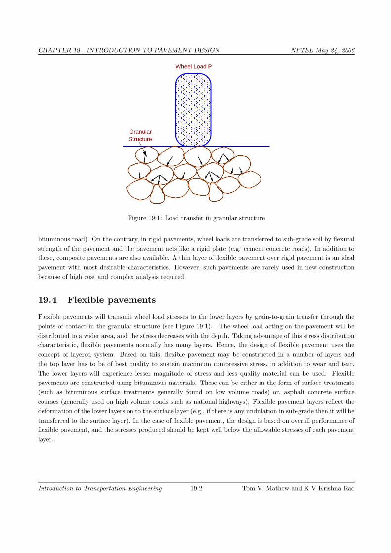
CHAPTER 19. INTRODUCTION TO PAVEMENT DESIGN NPTEL May 24, 2006
���������������������������������������������������������������������������������������������������������������������������������������������������������������������������������������������������������������������������������������������������������������������������������������������������������������������������������������������������������������������������������������������������������������������������������������������������
���������������������������������������������������������������������������������������������������������������������������������������������������������������������������������������������������������������������������������������������������������������������������������������������������������������������������������������������������������������������������������������������������������������������
Granular Structure
Wheel Load P
Figure 19:1: Load transfer in granular structure
bituminous road). On the contrary, in rigid pavements, wheel loads are transferred to sub-grade soil by flexural
strength of the pavement and the pavement acts like a rigid plate (e.g. cement concrete roads). In addition to
these, composite pavements are also available. A thin layer of flexible pavement over rigid pavement is an ideal
pavement with most desirable characteristics. However, such pavements are rarely used in new construction
because of high cost and complex analysis required.
19.4 Flexible pavements
Flexible pavements will transmit wheel load stresses to the lower layers by grain-to-grain transfer through the
points of contact in the granular structure (see Figure 19:1). The wheel load acting on the pavement will be
distributed to a wider area, and the stress decreases with the depth. Taking advantage of this stress distribution
characteristic, flexible pavements normally has many layers. Hence, the design of flexible pavement uses the
concept of layered system. Based on this, flexible pavement may be constructed in a number of layers and
the top layer has to be of best quality to sustain maximum compressive stress, in addition to wear and tear.
The lower layers will experience lesser magnitude of stress and less quality material can be used. Flexible
pavements are constructed using bituminous materials. These can be either in the form of surface treatments
(such as bituminous surface treatments generally found on low volume roads) or, asphalt concrete surface
courses (generally used on high volume roads such as national highways). Flexible pavement layers reflect the
deformation of the lower layers on to the surface layer (e.g., if there is any undulation in sub-grade then it will be
transferred to the surface layer). In the case of flexible pavement, the design is based on overall performance of
flexible pavement, and the stresses produced should be kept well below the allowable stresses of each pavement
layer.
Introduction to Transportation Engineering 19.2 Tom V. Mathew and K V Krishna Rao
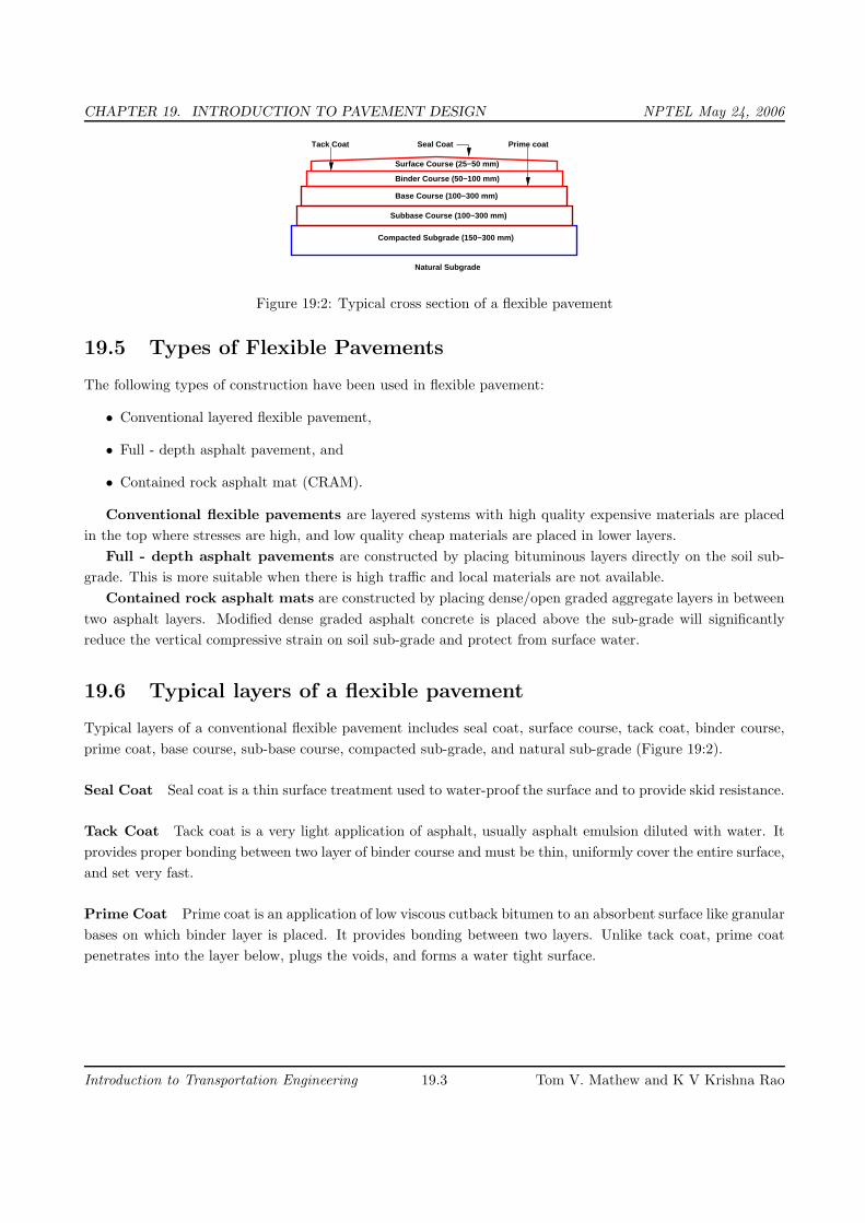
CHAPTER 19. INTRODUCTION TO PAVEMENT DESIGN NPTEL May 24, 2006
Tack Coat
Surface Course (25−50 mm)
Base Course (100−300 mm)
Binder Course (50−100 mm)
Subbase Course (100−300 mm)
Compacted Subgrade (150−300 mm)
Natural Subgrade
Seal Coat Prime coat
Figure 19:2: Typical cross section of a flexible pavement
19.5 Types of Flexible Pavements
The following types of construction have been used in flexible pavement:
• Conventional layered flexible pavement,
• Full - depth asphalt pavement, and
• Contained rock asphalt mat (CRAM).
Conventional flexible pavements are layered systems with high quality expensive materials are placed
in the top where stresses are high, and low quality cheap materials are placed in lower layers.
Full - depth asphalt pavements are constructed by placing bituminous layers directly on the soil sub-
grade. This is more suitable when there is high traffic and local materials are not available.
Contained rock asphalt mats are constructed by placing dense/open graded aggregate layers in between
two asphalt layers. Modified dense graded asphalt concrete is placed above the sub-grade will significantly
reduce the vertical compressive strain on soil sub-grade and protect from surface water.
19.6 Typical layers of a flexible pavement
Typical layers of a conventional flexible pavement includes seal coat, surface course, tack coat, binder course,
prime coat, base course, sub-base course, compacted sub-grade, and natural sub-grade (Figure 19:2).
Seal Coat Seal coat is a thin surface treatment used to water-proof the surface and to provide skid resistance.
Tack Coat Tack coat is a very light application of asphalt, usually asphalt emulsion diluted with water. It
provides proper bonding between two layer of binder course and must be thin, uniformly cover the entire surface,
and set very fast.
Prime Coat Prime coat is an application of low viscous cutback bitumen to an absorbent surface like granular
bases on which binder layer is placed. It provides bonding between two layers. Unlike tack coat, prime coat
penetrates into the layer below, plugs the voids, and forms a water tight surface.
Introduction to Transportation Engineering 19.3 Tom V. Mathew and K V Krishna Rao
CHAPTER 19. INTRODUCTION TO PAVEMENT DESIGN NPTEL May 24, 2006
Surface course
Surface course is the layer directly in contact with traffic loads and generally contains superior quality materials.
They are usually constructed with dense graded asphalt concrete(AC). The functions and requirements of this
layer are:
• It provides characteristics such as friction, smoothness, drainage, etc. Also it will prevent the entrance of
excessive quantities of surface water into the underlying base, sub-base and sub-grade
• It must be tough to resist the distortion under traffic and provide a smooth and skid- resistant riding
surface
• It must be water proof to protect the entire base and sub-grade from the weakening effect of water
Binder course
This layer provides the bulk of the asphalt concrete structure. It’s chief purpose is to distribute load to the base
course The binder course generally consists of aggregates having less asphalt and doesn’t require quality as high
as the surface course, so replacing a part of the surface course by the binder course results in more economical
design
Base course
The base course is the layer of material immediately beneath the surface of binder course and it provides
additional load distribution and contributes to the sub-surface drainage It may be composed of crushed stone,
crushed slag, and other untreated or stabilized materials
Sub-Base course
The sub-base course is the layer of material beneath the base course and the primary functions are to provide
structural support, improve drainage and reduce the intrusion of fines from the sub-grade in the pavement
structure If the base course is open graded, then the sub-base course with more fines can serve as a filler
between sub-grade and the base course A sub-base course is not always needed or used. For example, a
pavement constructed over a high quality, stiff sub-grade may not need the additional features offered by a
sub-base course. In such situations, sub-base course may not be provided
Sub-grade
The top soil or sub-grade is a layer of natural soil prepared to receive the stresses from the layers above It is
essential that at no time soil sub-grade is overstressed It should be compacted to the desirable density, near the
optimum moisture content
19.7 Failure of flexible pavements
The major flexible pavement failures are fatigue cracking, rutting, and thermal cracking. The fatigue cracking
of flexible pavement is due to horizontal tensile strain at the bottom of the asphaltic concrete. The failure
criterion relates allowable number of load repetitions to tensile strain and this relation can be determined in the
Introduction to Transportation Engineering 19.4 Tom V. Mathew and K V Krishna Rao
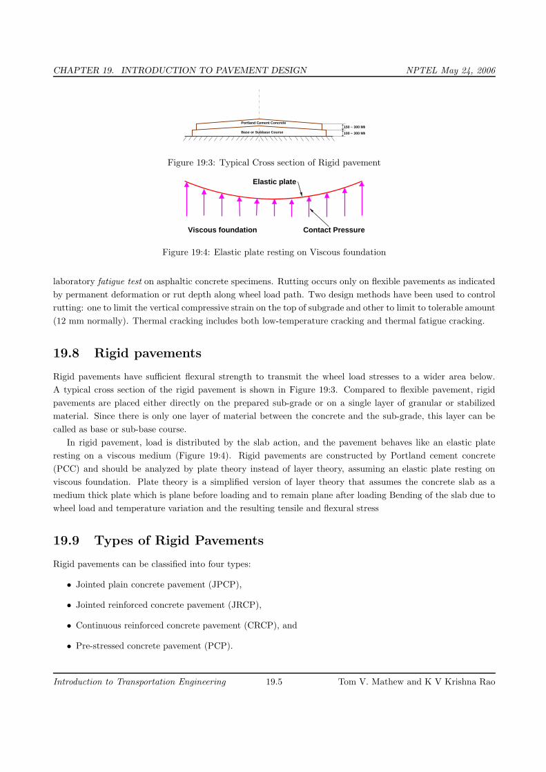
CHAPTER 19. INTRODUCTION TO PAVEMENT DESIGN NPTEL May 24, 2006
Base or Subbase Course
Portland Cement Concrete150 − 300 MM
100 − 300 MM
Figure 19:3: Typical Cross section of Rigid pavement
Elastic plate
Viscous foundation Contact Pressure
Figure 19:4: Elastic plate resting on Viscous foundation
laboratory fatigue test on asphaltic concrete specimens. Rutting occurs only on flexible pavements as indicated
by permanent deformation or rut depth along wheel load path. Two design methods have been used to control
rutting: one to limit the vertical compressive strain on the top of subgrade and other to limit to tolerable amount
(12 mm normally). Thermal cracking includes both low-temperature cracking and thermal fatigue cracking.
19.8 Rigid pavements
Rigid pavements have sufficient flexural strength to transmit the wheel load stresses to a wider area below.
A typical cross section of the rigid pavement is shown in Figure 19:3. Compared to flexible pavement, rigid
pavements are placed either directly on the prepared sub-grade or on a single layer of granular or stabilized
material. Since there is only one layer of material between the concrete and the sub-grade, this layer can be
called as base or sub-base course.
In rigid pavement, load is distributed by the slab action, and the pavement behaves like an elastic plate
resting on a viscous medium (Figure 19:4). Rigid pavements are constructed by Portland cement concrete
(PCC) and should be analyzed by plate theory instead of layer theory, assuming an elastic plate resting on
viscous foundation. Plate theory is a simplified version of layer theory that assumes the concrete slab as a
medium thick plate which is plane before loading and to remain plane after loading Bending of the slab due to
wheel load and temperature variation and the resulting tensile and flexural stress
19.9 Types of Rigid Pavements
Rigid pavements can be classified into four types:
• Jointed plain concrete pavement (JPCP),
• Jointed reinforced concrete pavement (JRCP),
• Continuous reinforced concrete pavement (CRCP), and
• Pre-stressed concrete pavement (PCP).
Introduction to Transportation Engineering 19.5 Tom V. Mathew and K V Krishna Rao
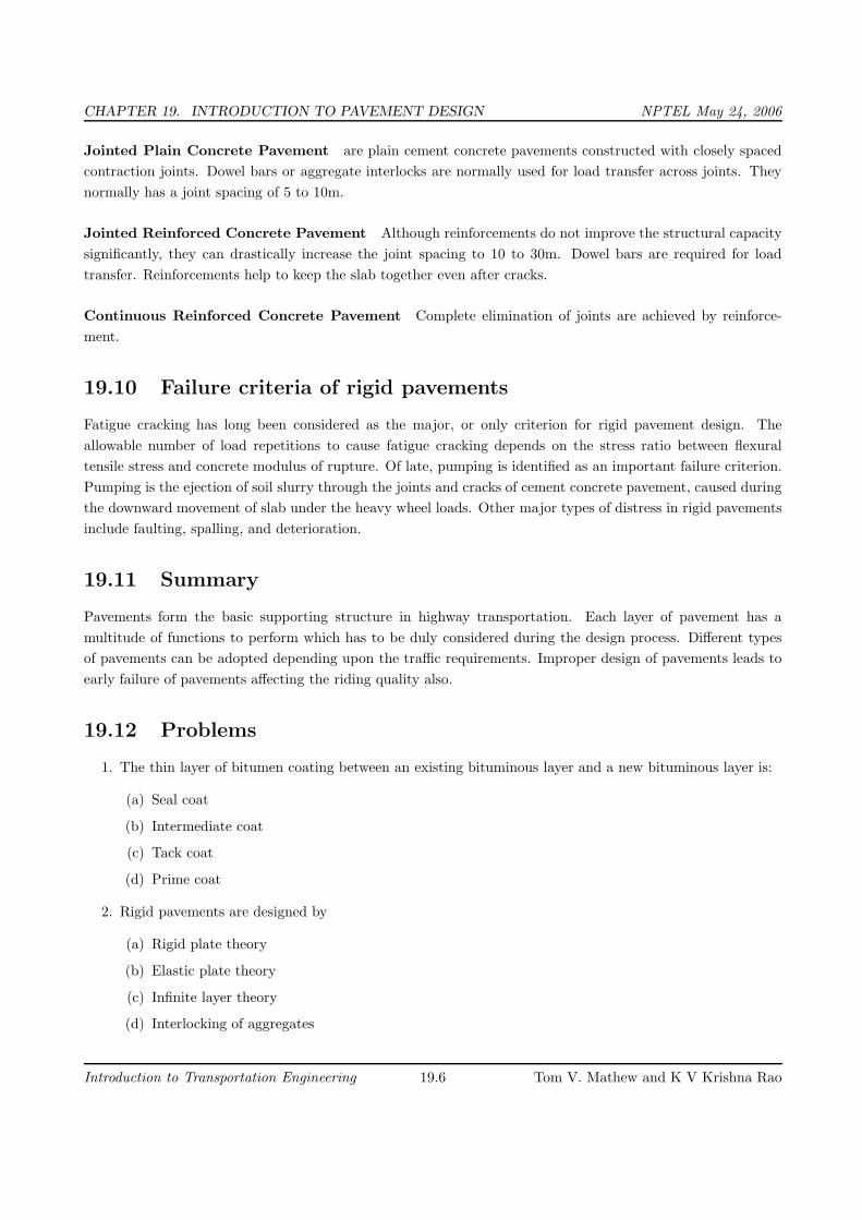
CHAPTER 19. INTRODUCTION TO PAVEMENT DESIGN NPTEL May 24, 2006
Jointed Plain Concrete Pavement are plain cement concrete pavements constructed with closely spaced
contraction joints. Dowel bars or aggregate interlocks are normally used for load transfer across joints. They
normally has a joint spacing of 5 to 10m.
Jointed Reinforced Concrete Pavement Although reinforcements do not improve the structural capacity
significantly, they can drastically increase the joint spacing to 10 to 30m. Dowel bars are required for load
transfer. Reinforcements help to keep the slab together even after cracks.
Continuous Reinforced Concrete Pavement Complete elimination of joints are achieved by reinforce-
ment.
19.10 Failure criteria of rigid pavements
Fatigue cracking has long been considered as the major, or only criterion for rigid pavement design. The
allowable number of load repetitions to cause fatigue cracking depends on the stress ratio between flexural
tensile stress and concrete modulus of rupture. Of late, pumping is identified as an important failure criterion.
Pumping is the ejection of soil slurry through the joints and cracks of cement concrete pavement, caused during
the downward movement of slab under the heavy wheel loads. Other major types of distress in rigid pavements
include faulting, spalling, and deterioration.
19.11 Summary
Pavements form the basic supporting structure in highway transportation. Each layer of pavement has a
multitude of functions to perform which has to be duly considered during the design process. Different types
of pavements can be adopted depending upon the traffic requirements. Improper design of pavements leads to
early failure of pavements affecting the riding quality also.
19.12 Problems
1. The thin layer of bitumen coating between an existing bituminous layer and a new bituminous layer is:
(a) Seal coat
(b) Intermediate coat
(c) Tack coat
(d) Prime coat
2. Rigid pavements are designed by
(a) Rigid plate theory
(b) Elastic plate theory
(c) Infinite layer theory
(d) Interlocking of aggregates
Introduction to Transportation Engineering 19.6 Tom V. Mathew and K V Krishna Rao
CHAPTER 19. INTRODUCTION TO PAVEMENT DESIGN NPTEL May 24, 2006
19.13 Solutions
1. The thin layer of bitumen coating between an existing bituminous layer and a new bituminous layer is:
(a) Seal coat
(b) Intermediate coat
(c) Tack coat√
(d) Prime coat
2. Rigid pavements are designed by
(a) Rigid plate theory
(b) Elastic plate theory√
(c) Infinite layer theory
(d) Interlocking of aggregates
Introduction to Transportation Engineering 19.7 Tom V. Mathew and K V Krishna Rao
CHAPTER 20. FACTORS AFFECTING PAVEMENT DESIGN NPTEL May 24, 2006
Chapter 20
Factors affecting pavement design
20.1 Overview
In the previous chapter we had discussed about the types of pavements and their failure criteria. There are
many factors that affect pavement design which can be classified into four categories as traffic and loading,
structural models, material characterization, environment. They will be discussed in detail in this chapter.
20.2 Traffic and loading
Traffic is the most important factor in the pavement design. The key factors include contact pressure, wheel
load, axle configuration, moving loads, load, and load repetitions.
Contact pressure The tyre pressure is an important factor, as it determine the contact area and the contact
pressure between the wheel and the pavement surface. Even though the shape of the contact area is elliptical,
for sake of simplicity in analysis, a circular area is often considered.
Wheel load The next important factor is the wheel load which determines the depth of the pavement required
to ensure that the subgrade soil is not failed. Wheel configuration affect the stress distribution and deflection
within a pavemnet. Many commercial vehicles have dual rear wheels which ensure that the contact pressure is
within the limits. The normal practice is to convert dual wheel into an equivalent single wheel load so that the
analysis is made simpler.
Axle configuration The load carrying capacity of the commercial vehicle is further enhanced by the intro-
duction of multiple axles.
Moving loads The damage to the pavement is much higher if the vehicle is moving at creep speed. Many
studies show that when the speed is increased from 2 km/hr to 24 km/hr, the stresses and deflection reduced
by 40 per cent.
Repetition of Loads The influence of traffic on pavement not only depend on the magnitude of the wheel
load, but also on the frequency of the load applications. Each load application causes some deformation and the
total deformation is the summation of all these. Although the pavement deformation due to single axle load is
very small, the cumulative effect of number of load repetition is significant. Therefore, modern design is based
on total number of standard axle load (usually 80 kN single axle).
Introduction to Transportation Engineering 20.1 Tom V. Mathew and K V Krishna Rao
CHAPTER 20. FACTORS AFFECTING PAVEMENT DESIGN NPTEL May 24, 2006
20.3 Structural models
The structural models are various analysis approaches to determine the pavement responses (stresses, strains,
and deflections) at various locations in a pavement due to the application of wheel load. The most common
structural models are layered elastic model and visco-elastic models.
Layered elastic model A layered elastic model can compute stresses, strains, and deflections at any point
in a pavement structure resulting from the application of a surface load. Layered elastic models assume that
each pavement structural layer is homogeneous, isotropic, and linearly elastic. In other words, the material
properties are same at every point in a given layer and the layer will rebound to its original form once the load
is removed. The layered elastic approach works with relatively simple mathematical models that relates stress,
strain, and deformation with wheel loading and material properties like modulus of elasticity and poissons ratio.
20.4 Material characterization
The following material properties should be specified for both flexible and rigid pavements.
• When pavements are considered as linear elastic, the elastic moduli and poisson ratio of subgrade and
each component layer must be specified.
• If the elastic modulus of a material varies with the time of loading, then the resilient modulus, which is
elastic modulus under repeated loads, must be selected in accordance with a load duration corresponding
to the vehicle speed.
• When a material is considered non-linear elastic, the constitutive equation relating the resilient modulus
to the state of the stress must be provided.
20.5 Environmental factors
Environmental factors affect the performance of the pavement materials and cause various damages. Environ-
mental factors that affect pavement are of two types, temperature and precipitation and they are discussed
below:
20.5.1 Temperature
The effect of temperature on asphalt pavements is different from that of concrete pavements. Temperature
affects the resilient modulus of asphalt layers, while it induces curling of concrete slab. In rigid pavements, due
to difference in temperatures of top and bottom of slab, temperature stresses or frictional stresses are developed.
While in flexible pavement, dynamic modulus of asphaltic concrete varies with temperature. Frost heave causes
differential settlements and pavement roughness. The most detrimental effect of frost penetration occurs during
the spring break up period when the ice melts and subgrade is a saturated condition.
20.5.2 Precipitation
The precipitation from rain and snow affects the quantity of surface water infiltrating into the subgrade and
the depth of ground water table. Poor drainage may bring lack of shear strength, pumping, loss of support, etc.
Introduction to Transportation Engineering 20.2 Tom V. Mathew and K V Krishna Rao
CHAPTER 20. FACTORS AFFECTING PAVEMENT DESIGN NPTEL May 24, 2006
20.6 Summary
Several factors affecting pavement design were discussed, the most important being wheel load. Since pavements
are designed to take moving loads, slow moving loads and static loads can be detrimental to the pavement.
Temperature also influences pavement design especially the frost action which is very important in cold countries.
20.7 Problems
1. Factor that least affect the pavement is
(a) Speed of vehicles
(b) Wheel load
(c) Axle configuration
(d) Load repetition
2. Standard axle load is
(a) 40kN
(b) 60kN
(c) 80kN
(d) 10kN
20.8 Solutions
1. Factor that least affect the pavement is
(a) Speed of vehicles√
(b) Wheel load
(c) Axle configuration
(d) Load repetition
2. Standard axle load is
(a) 40kN
(b) 60kN
(c) 80kN√
(d) 10kN
Introduction to Transportation Engineering 20.3 Tom V. Mathew and K V Krishna Rao
CHAPTER 21. PAVEMENT MATERIALS: SOIL NPTEL May 24, 2006
Chapter 21
Pavement materials: Soil
21.1 Overview
Pavements are a conglomeration of materials. These materials, their associated properties, and their interactions
determine the properties of the resultant pavement. Thus, a good understanding of these materials, how they
are characterized, and how they perform is fundamental to understanding pavement. The materials which are
used in the construction of highway are of intense interest to the highway engineer. This requires not only a
thorough understanding of the soil and aggregate properties which affect pavement stability and durability, but
also the binding materials which may be added to improve these pavement features.
21.2 Sub grade soil
Soil is an accumulation or deposit of earth material, derived naturally from the disintegration of rocks or
decay of vegetation, that can be excavated readily with power equipment in the field or disintegrated by gentle
mechanical means in the laboratory. The supporting soil beneath pavement and its special under courses is
called sub grade. Undisturbed soil beneath the pavement is called natural sub grade. Compacted sub grade is
the soil compacted by controlled movement of heavy compactors.
21.2.1 Desirable properties
The desirable properties of sub grade soil as a highway material are
• Stability
• Incompressibility
• Permanency of strength
• Minimum changes in volume and stability under adverse conditions of weather and ground water
• Good drainage, and
• Ease of compaction
Introduction to Transportation Engineering 21.1 Tom V. Mathew and K V Krishna Rao
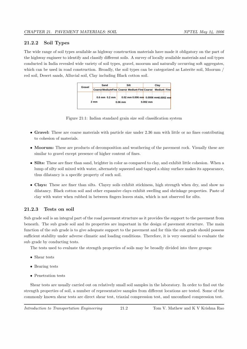
CHAPTER 21. PAVEMENT MATERIALS: SOIL NPTEL May 24, 2006
21.2.2 Soil Types
The wide range of soil types available as highway construction materials have made it obligatory on the part of
the highway engineer to identify and classify different soils. A survey of locally available materials and soil types
conducted in India revealed wide variety of soil types, gravel, moorum and naturally occurring soft aggregates,
which can be used in road construction. Broadly, the soil types can be categorized as Laterite soil, Moorum /
red soil, Desert sands, Alluvial soil, Clay including Black cotton soil.
GravelSand Silt Clay
FineMediumCoarseFineMediumCoarseFineMediumCoarse
0.2 mm
2 mm
0.02 mm 0.006 mm0.6 mm 0.0006 mm0.0002 mm
0.06 mm 0.002 mm
Figure 21:1: Indian standard grain size soil classification system
• Gravel: These are coarse materials with particle size under 2.36 mm with little or no fines contributing
to cohesion of materials.
• Moorum: These are products of decomposition and weathering of the pavement rock. Visually these are
similar to gravel except presence of higher content of fines.
• Silts: These are finer than sand, brighter in color as compared to clay, and exhibit little cohesion. When a
lump of silty soil mixed with water, alternately squeezed and tapped a shiny surface makes its appearance,
thus dilatancy is a specific property of such soil.
• Clays: These are finer than silts. Clayey soils exhibit stickiness, high strength when dry, and show no
dilatancy. Black cotton soil and other expansive clays exhibit swelling and shrinkage properties. Paste of
clay with water when rubbed in between fingers leaves stain, which is not observed for silts.
21.2.3 Tests on soil
Sub grade soil is an integral part of the road pavement structure as it provides the support to the pavement from
beneath. The sub grade soil and its properties are important in the design of pavement structure. The main
function of the sub grade is to give adequate support to the pavement and for this the sub grade should possess
sufficient stability under adverse climatic and loading conditions. Therefore, it is very essential to evaluate the
sub grade by conducting tests.
The tests used to evaluate the strength properties of soils may be broadly divided into three groups:
• Shear tests
• Bearing tests
• Penetration tests
Shear tests are usually carried out on relatively small soil samples in the laboratory. In order to find out the
strength properties of soil, a number of representative samples from different locations are tested. Some of the
commonly known shear tests are direct shear test, triaxial compression test, and unconfined compression test.
Introduction to Transportation Engineering 21.2 Tom V. Mathew and K V Krishna Rao
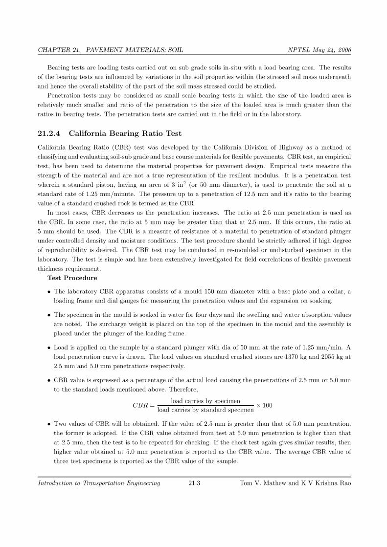
CHAPTER 21. PAVEMENT MATERIALS: SOIL NPTEL May 24, 2006
Bearing tests are loading tests carried out on sub grade soils in-situ with a load bearing area. The results
of the bearing tests are influenced by variations in the soil properties within the stressed soil mass underneath
and hence the overall stability of the part of the soil mass stressed could be studied.
Penetration tests may be considered as small scale bearing tests in which the size of the loaded area is
relatively much smaller and ratio of the penetration to the size of the loaded area is much greater than the
ratios in bearing tests. The penetration tests are carried out in the field or in the laboratory.
21.2.4 California Bearing Ratio Test
California Bearing Ratio (CBR) test was developed by the California Division of Highway as a method of
classifying and evaluating soil-sub grade and base course materials for flexible pavements. CBR test, an empirical
test, has been used to determine the material properties for pavement design. Empirical tests measure the
strength of the material and are not a true representation of the resilient modulus. It is a penetration test
wherein a standard piston, having an area of 3 in2 (or 50 mm diameter), is used to penetrate the soil at a
standard rate of 1.25 mm/minute. The pressure up to a penetration of 12.5 mm and it’s ratio to the bearing
value of a standard crushed rock is termed as the CBR.
In most cases, CBR decreases as the penetration increases. The ratio at 2.5 mm penetration is used as
the CBR. In some case, the ratio at 5 mm may be greater than that at 2.5 mm. If this occurs, the ratio at
5 mm should be used. The CBR is a measure of resistance of a material to penetration of standard plunger
under controlled density and moisture conditions. The test procedure should be strictly adhered if high degree
of reproducibility is desired. The CBR test may be conducted in re-moulded or undisturbed specimen in the
laboratory. The test is simple and has been extensively investigated for field correlations of flexible pavement
thickness requirement.
Test Procedure
• The laboratory CBR apparatus consists of a mould 150 mm diameter with a base plate and a collar, a
loading frame and dial gauges for measuring the penetration values and the expansion on soaking.
• The specimen in the mould is soaked in water for four days and the swelling and water absorption values
are noted. The surcharge weight is placed on the top of the specimen in the mould and the assembly is
placed under the plunger of the loading frame.
• Load is applied on the sample by a standard plunger with dia of 50 mm at the rate of 1.25 mm/min. A
load penetration curve is drawn. The load values on standard crushed stones are 1370 kg and 2055 kg at
2.5 mm and 5.0 mm penetrations respectively.
• CBR value is expressed as a percentage of the actual load causing the penetrations of 2.5 mm or 5.0 mm
to the standard loads mentioned above. Therefore,
CBR =load carries by specimen
load carries by standard specimen× 100
• Two values of CBR will be obtained. If the value of 2.5 mm is greater than that of 5.0 mm penetration,
the former is adopted. If the CBR value obtained from test at 5.0 mm penetration is higher than that
at 2.5 mm, then the test is to be repeated for checking. If the check test again gives similar results, then
higher value obtained at 5.0 mm penetration is reported as the CBR value. The average CBR value of
three test specimens is reported as the CBR value of the sample.
Introduction to Transportation Engineering 21.3 Tom V. Mathew and K V Krishna Rao
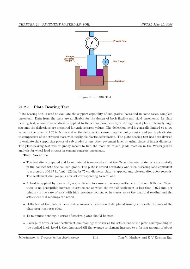
CHAPTER 21. PAVEMENT MATERIALS: SOIL NPTEL May 24, 2006
Specimen
Dial Guage
Proving Ring
PlungerSurcharge Weight
Figure 21:2: CBR Test
21.2.5 Plate Bearing Test
Plate bearing test is used to evaluate the support capability of sub-grades, bases and in some cases, complete
pavement. Data from the tests are applicable for the design of both flexible and rigid pavements. In plate
bearing test, a compressive stress is applied to the soil or pavement layer through rigid plates relatively large
size and the deflections are measured for various stress values. The deflection level is generally limited to a low
value, in the order of 1.25 to 5 mm and so the deformation caused may be partly elastic and partly plastic due
to compaction of the stressed mass with negligible plastic deformation. The plate-bearing test has been devised
to evaluate the supporting power of sub grades or any other pavement layer by using plates of larger diameter.
The plate-bearing test was originally meant to find the modulus of sub grade reaction in the Westergaard’s
analysis for wheel load stresses in cement concrete pavements.
Test Procedure
• The test site is prepared and loose material is removed so that the 75 cm diameter plate rests horizontally
in full contact with the soil sub-grade. The plate is seated accurately and then a seating load equivalent
to a pressure of 0.07 kg/cm2 (320 kg for 75 cm diameter plate) is applied and released after a few seconds.
The settlement dial gauge is now set corresponding to zero load.
• A load is applied by means of jack, sufficient to cause an average settlement of about 0.25 cm. When
there is no perceptible increase in settlement or when the rate of settlement is less than 0.025 mm per
minute (in the case of soils with high moisture content or in clayey soils) the load dial reading and the
settlement dial readings are noted.
• Deflection of the plate is measured by means of deflection dials; placed usually at one-third points of the
plate near it’s outer edge.
• To minimize bending, a series of stacked plates should be used.
• Average of three or four settlement dial readings is taken as the settlement of the plate corresponding to
the applied load. Load is then increased till the average settlement increase to a further amount of about
Introduction to Transportation Engineering 21.4 Tom V. Mathew and K V Krishna Rao
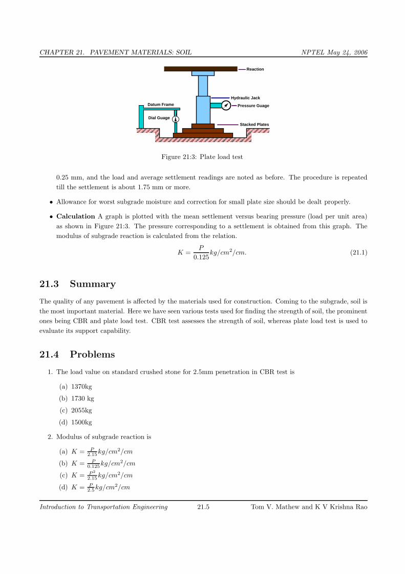
CHAPTER 21. PAVEMENT MATERIALS: SOIL NPTEL May 24, 2006
������������������������������������������������������������������������������������������������������������������������������������������������������������������������������������������������������������������������������������������������������������������������������������������������������������
������������������������������������������������������������������������������������������������������������������������������������������������������������������������������������������������������������������������������������������������������������������������������������������������������������
Datum Frame
Reaction
Hydraulic Jack
Pressure Guage
Stacked Plates
Dial Guage
Figure 21:3: Plate load test
0.25 mm, and the load and average settlement readings are noted as before. The procedure is repeated
till the settlement is about 1.75 mm or more.
• Allowance for worst subgrade moisture and correction for small plate size should be dealt properly.
• Calculation A graph is plotted with the mean settlement versus bearing pressure (load per unit area)
as shown in Figure 21:3. The pressure corresponding to a settlement is obtained from this graph. The
modulus of subgrade reaction is calculated from the relation.
K =P
0.125kg/cm2/cm. (21.1)
21.3 Summary
The quality of any pavement is affected by the materials used for construction. Coming to the subgrade, soil is
the most important material. Here we have seen various tests used for finding the strength of soil, the prominent
ones being CBR and plate load test. CBR test assesses the strength of soil, whereas plate load test is used to
evaluate its support capability.
21.4 Problems
1. The load value on standard crushed stone for 2.5mm penetration in CBR test is
(a) 1370kg
(b) 1730 kg
(c) 2055kg
(d) 1500kg
2. Modulus of subgrade reaction is
(a) K = P
2.15kg/cm2/cm
(b) K = P
0.125kg/cm2/cm
(c) K = P2
2.15kg/cm2/cm
(d) K = P
2.5kg/cm2/cm
Introduction to Transportation Engineering 21.5 Tom V. Mathew and K V Krishna Rao
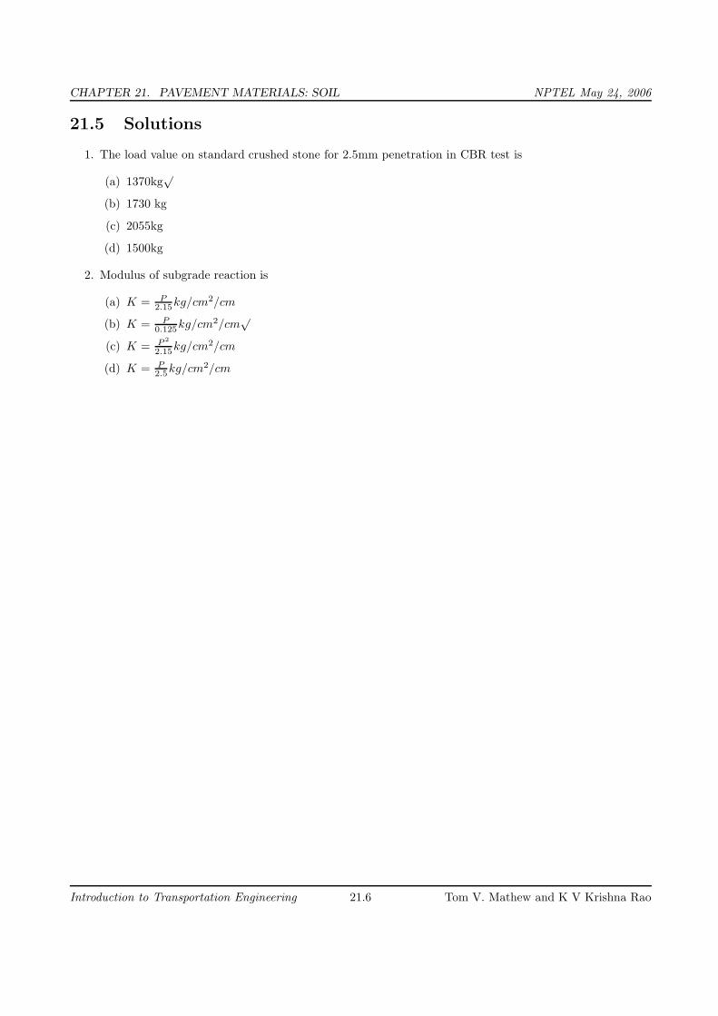
CHAPTER 21. PAVEMENT MATERIALS: SOIL NPTEL May 24, 2006
21.5 Solutions
1. The load value on standard crushed stone for 2.5mm penetration in CBR test is
(a) 1370kg√
(b) 1730 kg
(c) 2055kg
(d) 1500kg
2. Modulus of subgrade reaction is
(a) K = P
2.15kg/cm2/cm
(b) K = P
0.125kg/cm2/cm
√
(c) K = P2
2.15kg/cm2/cm
(d) K = P
2.5kg/cm2/cm
Introduction to Transportation Engineering 21.6 Tom V. Mathew and K V Krishna Rao
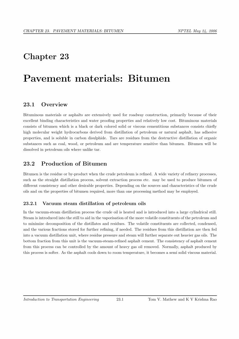
CHAPTER 23. PAVEMENT MATERIALS: BITUMEN NPTEL May 24, 2006
Chapter 23
Pavement materials: Bitumen
23.1 Overview
Bituminous materials or asphalts are extensively used for roadway construction, primarily because of their
excellent binding characteristics and water proofing properties and relatively low cost. Bituminous materials
consists of bitumen which is a black or dark colored solid or viscous cementitious substances consists chiefly
high molecular weight hydrocarbons derived from distillation of petroleum or natural asphalt, has adhesive
properties, and is soluble in carbon disulphide. Tars are residues from the destructive distillation of organic
substances such as coal, wood, or petroleum and are temperature sensitive than bitumen. Bitumen will be
dissolved in petroleum oils where unlike tar.
23.2 Production of Bitumen
Bitumen is the residue or by-product when the crude petroleum is refined. A wide variety of refinery processes,
such as the straight distillation process, solvent extraction process etc. may be used to produce bitumen of
different consistency and other desirable properties. Depending on the sources and characteristics of the crude
oils and on the properties of bitumen required, more than one processing method may be employed.
23.2.1 Vacuum steam distillation of petroleum oils
In the vacuum-steam distillation process the crude oil is heated and is introduced into a large cylindrical still.
Steam is introduced into the still to aid in the vaporisation of the more volatile constituents of the petroleum and
to minimize decomposition of the distillates and residues. The volatile constituents are collected, condensed,
and the various fractions stored for further refining, if needed. The residues from this distillation are then fed
into a vacuum distillation unit, where residue pressure and steam will further separate out heavier gas oils. The
bottom fraction from this unit is the vacuum-steam-refined asphalt cement. The consistency of asphalt cement
from this process can be controlled by the amount of heavy gas oil removed. Normally, asphalt produced by
this process is softer. As the asphalt cools down to room temperature, it becomes a semi solid viscous material.
Introduction to Transportation Engineering 23.1 Tom V. Mathew and K V Krishna Rao
CHAPTER 23. PAVEMENT MATERIALS: BITUMEN NPTEL May 24, 2006
23.3 Different forms of bitumen
23.3.1 Cutback bitumen
Normal practice is to heat bitumen to reduce its viscosity. In some situations preference is given to use liquid
binders such as cutback bitumen. In cutback bitumen suitable solvent is used to lower the viscosity of the
bitumen. From the environmental point of view also cutback bitumen is preferred. The solvent from the
bituminous material will evaporate and the bitumen will bind the aggregate. Cutback bitumen is used for
cold weather bituminous road construction and maintenance. The distillates used for preparation of cutback
bitumen are naphtha, kerosene, diesel oil, and furnace oil. There are different types of cutback bitumen like
rapid curing (RC), medium curing (MC), and slow curing (SC). RC is recommended for surface dressing and
patchwork. MC is recommended for premix with less quantity of fine aggregates. SC is used for premix with
appreciable quantity of fine aggregates.
23.3.2 Bitumen Emulsion
Bitumen emulsion is a liquid product in which bitumen is suspended in a finely divided condition in an aqueous
medium and stabilized by suitable material. Normally cationic type emulsions are used in India. The bitumen
content in the emulsion is around 60% and the remaining is water. When the emulsion is applied on the road
it breaks down resulting in release of water and the mix starts to set. The time of setting depends upon the
grade of bitumen. The viscosity of bituminous emulsions can be measured as per IS: 8887-1995. Three types of
bituminous emulsions are available, which are Rapid setting (RS), Medium setting (MS), and Slow setting (SC).
Bitumen emulsions are ideal binders for hill road construction. Where heating of bitumen or aggregates are
difficult. Rapid setting emulsions are used for surface dressing work. Medium setting emulsions are preferred
for premix jobs and patch repairs work. Slow setting emulsions are preferred in rainy season.
23.3.3 Bituminous primers
In bituminous primer the distillate is absorbed by the road surface on which it is spread. The absorption therefore
depends on the porosity of the surface. Bitumen primers are useful on the stabilized surfaces and water bound
macadam base courses. Bituminous primers are generally prepared on road sites by mixing penetration bitumen
with petroleum distillate.
23.3.4 Modified Bitumen
Certain additives or blend of additives called as bitumen modifiers can improve properties of Bitumen and
bituminous mixes. Bitumen treated with these modifiers is known as modified bitumen. Polymer modified
bitumen (PMB)/ crumb rubber modified bitumen (CRMB) should be used only in wearing course depending
upon the requirements of extreme climatic variations. The detailed specifications for modified bitumen have
been issued by IRC: SP: 53-1999. It must be noted that the performance of PMB and CRMB is dependent on
strict control on temperature during construction. The advantages of using modified bitumen are as follows
• Lower susceptibility to daily and seasonal temperature variations
• Higher resistance to deformation at high pavement temperature
• Better age resistance properties
Introduction to Transportation Engineering 23.2 Tom V. Mathew and K V Krishna Rao
CHAPTER 23. PAVEMENT MATERIALS: BITUMEN NPTEL May 24, 2006
• Higher fatigue life for mixes
• Better adhesion between aggregates and binder
• Prevention of cracking and reflective cracking
23.4 Requirements of Bitumen
The desirable properties of bitumen depend on the mix type and construction. In general, Bitumen should
posses following desirable properties.
• The bitumen should not be highly temperature susceptible: during the hottest weather the mix should
not become too soft or unstable, and during cold weather the mix should not become too brittle causing
cracks.
• The viscosity of the bitumen at the time of mixing and compaction should be adequate. This can be
achieved by use of cutbacks or emulsions of suitable grades or by heating the bitumen and aggregates
prior to mixing.
• There should be adequate affinity and adhesion between the bitumen and aggregates used in the mix.
23.5 Tests on bitumen
There are a number of tests to assess the properties of bituminous materials. The following tests are usually
conducted to evaluate different properties of bituminous materials.
1. Penetration test
2. Ductility test
3. Softening point test
4. Specific gravity test
5. Viscosity test
6. Flash and Fire point test
7. Float test
8. Water content test
9. Loss on heating test
Introduction to Transportation Engineering 23.3 Tom V. Mathew and K V Krishna Rao
CHAPTER 23. PAVEMENT MATERIALS: BITUMEN NPTEL May 24, 2006
23.5.1 Penetration test
It measures the hardness or softness of bitumen by measuring the depth in tenths of a millimeter to which a
standard loaded needle will penetrate vertically in 5 seconds. BIS had standardized the equipment and test
procedure. The penetrometer consists of a needle assembly with a total weight of 100g and a device for releasing
and locking in any position. The bitumen is softened to a pouring consistency, stirred thoroughly and poured
into containers at a depth at least 15 mm in excess of the expected penetration. The test should be conducted at
a specified temperature of 25o C. It may be noted that penetration value is largely influenced by any inaccuracy
with regards to pouring temperature, size of the needle, weight placed on the needle and the test temperature.
A grade of 40/50 bitumen means the penetration value is in the range 40 to 50 at standard test conditions. In
hot climates, a lower penetration grade is preferred. The Figure 23:1 shows a schematic Penetration Test setup.
Penetration
Figure 23:1: Penetration Test Setup
23.5.2 Ductility test
Ductility is the property of bitumen that permits it to undergo great deformation or elongation. Ductility is
defined as the distance in cm, to which a standard sample or briquette of the material will be elongated without
breaking. Dimension of the briquette thus formed is exactly 1 cm square. The bitumen sample is heated and
poured in the mould assembly placed on a plate. These samples with moulds are cooled in the air and then in
water bath at 27o C temperature. The excess bitumen is cut and the surface is leveled using a hot knife. Then
the mould with assembly containing sample is kept in water bath of the ductility machine for about 90 minutes.
The sides of the moulds are removed, the clips are hooked on the machine and the machine is operated. The
distance up to the point of breaking of thread is the ductility value which is reported in cm. The ductility value
gets affected by factors such as pouring temperature, test temperature, rate of pulling etc. A minimum ductility
value of 75 cm has been specified by the BIS. Figure 23:2 shows ductility moulds to be filled with bitumen.
23.5.3 Softening point test
Softening point denotes the temperature at which the bitumen attains a particular degree of softening under
the specifications of test. The test is conducted by using Ring and Ball apparatus. A brass ring containing test
sample of bitumen is suspended in liquid like water or glycerin at a given temperature. A steel ball is placed
upon the bitumen sample and the liquid medium is heated at a rate of 5o C per minute. Temperature is noted
when the softened bitumen touches the metal plate which is at a specified distance below. Generally, higher
softening point indicates lower temperature susceptibility and is preferred in hot climates. Figure 23:3 shows
Softening Point test setup.
Introduction to Transportation Engineering 23.4 Tom V. Mathew and K V Krishna Rao
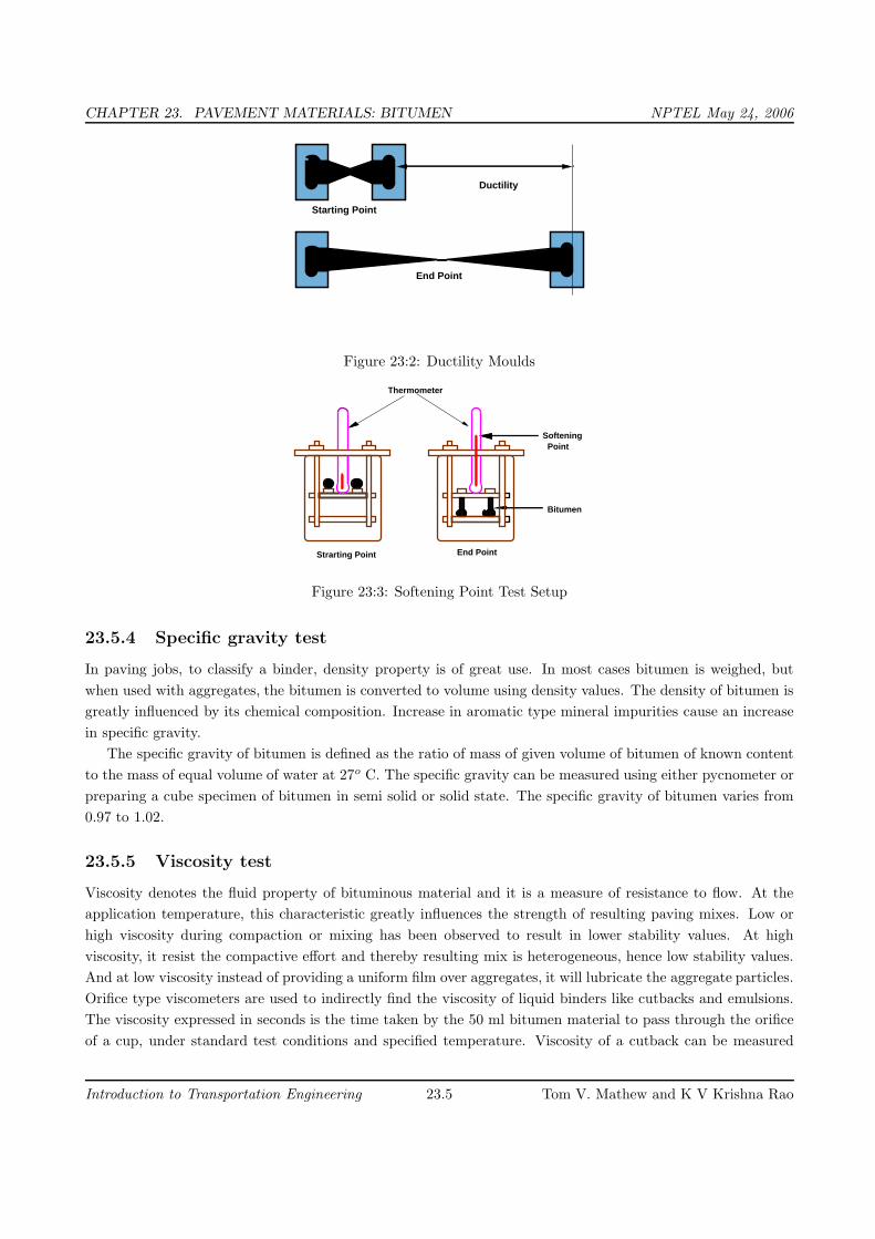
CHAPTER 23. PAVEMENT MATERIALS: BITUMEN NPTEL May 24, 2006
Ductility
Starting Point
End Point
Figure 23:2: Ductility Moulds
Strarting Point End Point
Bitumen
PointSoftening
Thermometer
Figure 23:3: Softening Point Test Setup
23.5.4 Specific gravity test
In paving jobs, to classify a binder, density property is of great use. In most cases bitumen is weighed, but
when used with aggregates, the bitumen is converted to volume using density values. The density of bitumen is
greatly influenced by its chemical composition. Increase in aromatic type mineral impurities cause an increase
in specific gravity.
The specific gravity of bitumen is defined as the ratio of mass of given volume of bitumen of known content
to the mass of equal volume of water at 27o C. The specific gravity can be measured using either pycnometer or
preparing a cube specimen of bitumen in semi solid or solid state. The specific gravity of bitumen varies from
0.97 to 1.02.
23.5.5 Viscosity test
Viscosity denotes the fluid property of bituminous material and it is a measure of resistance to flow. At the
application temperature, this characteristic greatly influences the strength of resulting paving mixes. Low or
high viscosity during compaction or mixing has been observed to result in lower stability values. At high
viscosity, it resist the compactive effort and thereby resulting mix is heterogeneous, hence low stability values.
And at low viscosity instead of providing a uniform film over aggregates, it will lubricate the aggregate particles.
Orifice type viscometers are used to indirectly find the viscosity of liquid binders like cutbacks and emulsions.
The viscosity expressed in seconds is the time taken by the 50 ml bitumen material to pass through the orifice
of a cup, under standard test conditions and specified temperature. Viscosity of a cutback can be measured
Introduction to Transportation Engineering 23.5 Tom V. Mathew and K V Krishna Rao
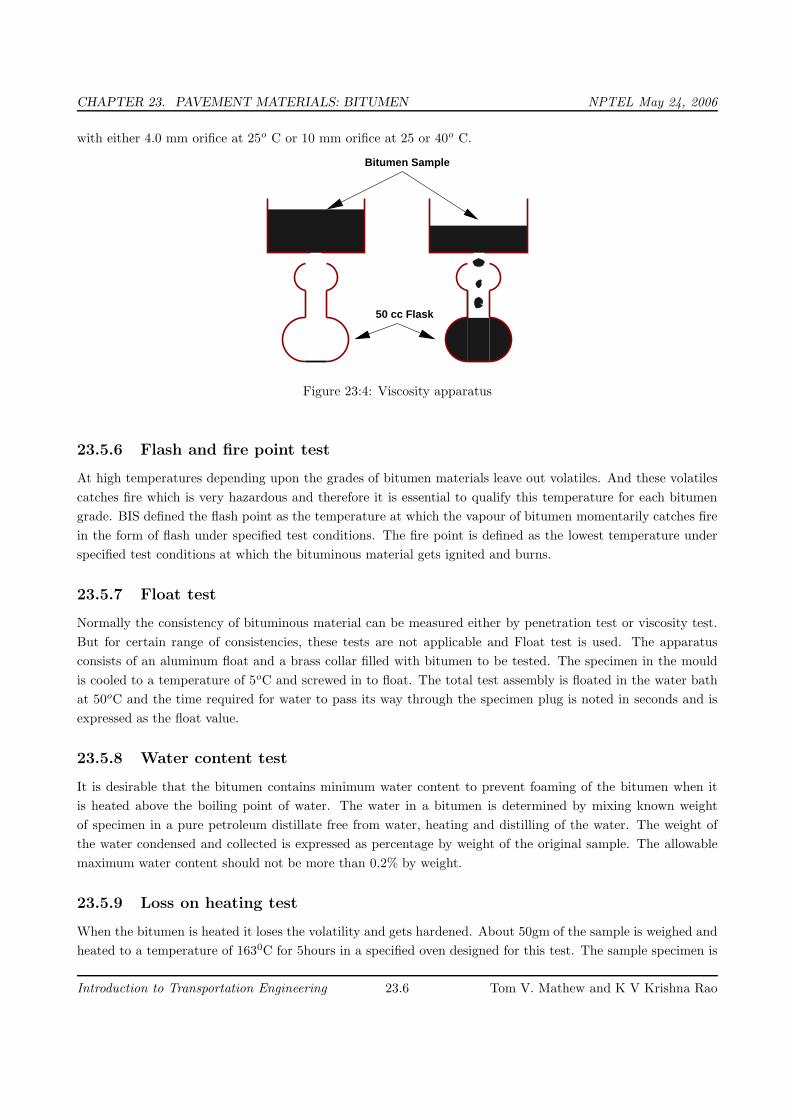
CHAPTER 23. PAVEMENT MATERIALS: BITUMEN NPTEL May 24, 2006
with either 4.0 mm orifice at 25o C or 10 mm orifice at 25 or 40o C.
Bitumen Sample
50 cc Flask
Figure 23:4: Viscosity apparatus
23.5.6 Flash and fire point test
At high temperatures depending upon the grades of bitumen materials leave out volatiles. And these volatiles
catches fire which is very hazardous and therefore it is essential to qualify this temperature for each bitumen
grade. BIS defined the flash point as the temperature at which the vapour of bitumen momentarily catches fire
in the form of flash under specified test conditions. The fire point is defined as the lowest temperature under
specified test conditions at which the bituminous material gets ignited and burns.
23.5.7 Float test
Normally the consistency of bituminous material can be measured either by penetration test or viscosity test.
But for certain range of consistencies, these tests are not applicable and Float test is used. The apparatus
consists of an aluminum float and a brass collar filled with bitumen to be tested. The specimen in the mould
is cooled to a temperature of 5oC and screwed in to float. The total test assembly is floated in the water bath
at 50oC and the time required for water to pass its way through the specimen plug is noted in seconds and is
expressed as the float value.
23.5.8 Water content test
It is desirable that the bitumen contains minimum water content to prevent foaming of the bitumen when it
is heated above the boiling point of water. The water in a bitumen is determined by mixing known weight
of specimen in a pure petroleum distillate free from water, heating and distilling of the water. The weight of
the water condensed and collected is expressed as percentage by weight of the original sample. The allowable
maximum water content should not be more than 0.2% by weight.
23.5.9 Loss on heating test
When the bitumen is heated it loses the volatility and gets hardened. About 50gm of the sample is weighed and
heated to a temperature of 1630C for 5hours in a specified oven designed for this test. The sample specimen is
Introduction to Transportation Engineering 23.6 Tom V. Mathew and K V Krishna Rao
CHAPTER 23. PAVEMENT MATERIALS: BITUMEN NPTEL May 24, 2006
Type of test Test Method
Penetration Test IS: 1203-1978
Ductility test IS: 1208-1978
Softening Point test IS: 1205-1978
Specific gravity test IS: 1202-1978
Viscosity test IS: 1206-1978
Flash and Fire Point test IS: 1209-1978
Float Test IS: 1210-1978
Determination of water content IS: 1211-1978
Determination of Loss on heating IS:1212-1978
Table 23:1: Tests for Bitumen with IS codes
weighed again after the heating period and loss in weight is expressed as percentage by weight of the original
sample. Bitumen used in pavement mixes should not indicate more than 1% loss in weight, but for bitumen
having penetration values 150-200 up to 2% loss in weight is allowed.
23.6 Summary
Requirements of bitumen as a binding material and its different forms were discussed. Various tests are con-
ducted on bitumen to assess its consistency, gradation, viscosity, temperature susceptibility, and safety. Standard
test procedures on bitumen were also covered in this chapter.
23.7 Problems
1. The minimum ductility value for bitumen specified by BIS is
(a) 50cm
(b) 25cm
(c) 75cm
(d) 100cm
2. The allowable maximum water content in bitumen should not be more than
(a) 2% by weight
(b) 0.2% by weight
(c) 2.5% by weight
(d) 5% by weight
23.8 Solutions
1. The minimum ductility value for bitumen specified by BIS is
Introduction to Transportation Engineering 23.7 Tom V. Mathew and K V Krishna Rao
CHAPTER 23. PAVEMENT MATERIALS: BITUMEN NPTEL May 24, 2006
(a) 50cm
(b) 25cm
(c) 75cm√
(d) 100cm
2. The allowable maximum water content in bitumen should not be more than
(a) 2% by weight
(b) 0.2% by weight√
(c) 2.5% by weight
(d) 5% by weight
Introduction to Transportation Engineering 23.8 Tom V. Mathew and K V Krishna Rao
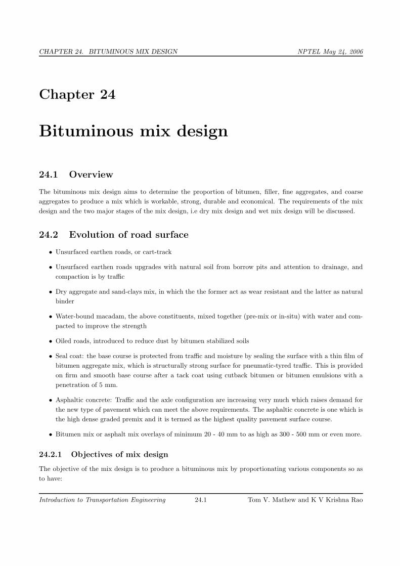
CHAPTER 24. BITUMINOUS MIX DESIGN NPTEL May 24, 2006
Chapter 24
Bituminous mix design
24.1 Overview
The bituminous mix design aims to determine the proportion of bitumen, filler, fine aggregates, and coarse
aggregates to produce a mix which is workable, strong, durable and economical. The requirements of the mix
design and the two major stages of the mix design, i.e dry mix design and wet mix design will be discussed.
24.2 Evolution of road surface
• Unsurfaced earthen roads, or cart-track
• Unsurfaced earthen roads upgrades with natural soil from borrow pits and attention to drainage, and
compaction is by traffic
• Dry aggregate and sand-clays mix, in which the the former act as wear resistant and the latter as natural
binder
• Water-bound macadam, the above constituents, mixed together (pre-mix or in-situ) with water and com-
pacted to improve the strength
• Oiled roads, introduced to reduce dust by bitumen stabilized soils
• Seal coat: the base course is protected from traffic and moisture by sealing the surface with a thin film of
bitumen aggregate mix, which is structurally strong surface for pneumatic-tyred traffic. This is provided
on firm and smooth base course after a tack coat using cutback bitumen or bitumen emulsions with a
penetration of 5 mm.
• Asphaltic concrete: Traffic and the axle configuration are increasing very much which raises demand for
the new type of pavement which can meet the above requirements. The asphaltic concrete is one which is
the high dense graded premix and it is termed as the highest quality pavement surface course.
• Bitumen mix or asphalt mix overlays of minimum 20 - 40 mm to as high as 300 - 500 mm or even more.
24.2.1 Objectives of mix design
The objective of the mix design is to produce a bituminous mix by proportionating various components so as
to have:
Introduction to Transportation Engineering 24.1 Tom V. Mathew and K V Krishna Rao
CHAPTER 24. BITUMINOUS MIX DESIGN NPTEL May 24, 2006
1. sufficient bitumen to ensure a durable pavement,
2. sufficient strength to resist shear deformation under traffic at higher temperature,
3. sufficient air voids in the compacted bitumen to allow for additional compaction by traffic,
4. sufficient workability to permit easy placement without segregation,
5. sufficient flexibility to avoid premature cracking due to repeated bending by traffic,and
6. sufficient flexibility at low temperature to prevent shrinkage cracks.
24.2.2 Constituents of a mix
• Coarse aggregates: Offer compressive and shear strength and shows good interlocking properties. E.g.
Granite
• Fine aggregates: Fills the voids in the coarse aggregate and stiffens the binder. E.g. Sand, Rock dust
• Filler: Fills the voids, stiffens the binder and offers permeability. E.g. Rock dust, cement, lime
• Binder: Fills the voids, cause particle adhesion and gluing and offers impermeability. E.g. Bitumen,
Asphalt, Tar
24.2.3 Types of mix
• Well-graded mix:- Dense mix, bituminous concrete has good proportion of all constituents and are
called dense bituminous macadam, offers good compressive strength and some tensile strength
• Gap-graded mix:- Some large coarse aggregates are missing and has good fatigue and tensile strength.
• Open-graded mix:- Fine aggregate and filler are missing, it is porous and offers good friction, low
strength and for high speed.
• Unbounded:- Binder is absent and behaves under loads as if its components were not linked together,
though good interlocking exists. Very low tensile strength and needs kerb protection.
24.2.4 Different layers in a pavement
• Bituminous base course Consist of mineral aggregate such as stone, gravel, or sand bonded together
by a bituminous material and used as a foundation upon which to place a binder or surface course.
• Bituminous binder course A bituminous-aggregate mixture used as an intermediate coarse between
the base and surface courses or as the first bituminous layer in a two-layer bituminous resurfacing. It is
sometimes called a leveling course.
• Asphaltic/Bituminous concrete Bituminous concrete consists of a mixture of aggregates continuously
graded from maximum size , typically less than 25 mm, through fine filler that is smaller than 0.075 mm.
Sufficient bitumen is added to the mix so that the compacted mix is effectively impervious and will have
acceptable dissipative and elastic properties.
Introduction to Transportation Engineering 24.2 Tom V. Mathew and K V Krishna Rao
CHAPTER 24. BITUMINOUS MIX DESIGN NPTEL May 24, 2006
Table 24:1: Aggregate gradation for BC
Sieve size Passing (%)
26.5 mm - 100
19. mm 90 - 100
9.5 mm 56 - 80
4.75 mm 35 - 65
2.36 mm 23 - 49
300 micron 5 - 19
75 micron 2 - 8
24.3 Requirements of Bituminous mixes
24.3.1 Stability
Stability is defined as the resistance of the paving mix to deformation under traffic load. Two examples of
failure are (i) shoving - a transverse rigid deformation which occurs at areas subject to severe acceleration and
(ii) grooving - longitudinal ridging due to channelization of traffic. Stability depend on the inter-particle friction,
primarily of the aggregates and the cohesion offered by the bitumen. Sufficient binder must be available to coat
all the particles at the same time should offer enough liquid friction. However, the stability decreases when the
binder content is high and when the particles are kept apart.
24.3.2 Durability
Durability is defined as the resistance of the mix against weathering and abrasive actions. Weathering causes
hardening due to loss of volatiles in the bitumen. Abrasion is due to wheel loads which causes tensile strains.
Typical examples of failure are (i) pot-holes, - deterioration of pavements locally and (ii) stripping, lost of binder
from the aggregates and aggregates are exposed. Disintegration is minimized by high binder content since they
cause the mix to be air and waterproof and the bitumen film is more resistant to hardening.
24.3.3 Flexibility
Flexibility is a measure of the level of bending strength needed to counteract traffic load and prevent cracking
of surface. Fracture is the cracks formed on the surface (hairline-cracks, alligator cracks), main reasons are
shrinkage and brittleness of the binder. Shrinkage cracks are due to volume change in the binder due to aging.
Brittleness is due to repeated bending of the surface due to traffic loads. Higher bitumen content will give
better flexibility and less fracture.
24.3.4 Skid resistance
It is the resistance of the finished pavement against skidding which depends on the surface texture and bitumen
content. It is an important factor in high speed traffic. Normally, an open graded coarse surface texture is
desirable.
Introduction to Transportation Engineering 24.3 Tom V. Mathew and K V Krishna Rao
CHAPTER 24. BITUMINOUS MIX DESIGN NPTEL May 24, 2006
24.3.5 Workability
Workability is the ease with which the mix can be laid and compacted, and formed to the required condition
and shape. This depends on the gradation of aggregates, their shape and texture, bitumen content and its
type. Angular, flaky, and elongated aggregates workability. On the other hand, rounded aggregates improve
workability.
24.3.6 Desirable properties
From the above discussion, the desirable properties of a bituminous mix can be summarized as follows:
• Stability to meet traffic demand
• Bitumen content to ensure proper binding and water proofing
• Voids to accommodate compaction due to traffic
• Flexibility to meet traffic loads, esp. in cold season
• Sufficient workability for construction
• Economical mix
24.4 Summary
Bituminous mixes should be stable, durable, flexible, workable and should offer sufficient skid resistance. The
mix consists of coarse and fine aggregates, filler and binder. It may be well graded, open graded, gap graded or
unbounded as per the requirements. As far as possible, it should be economical also.
24.5 Problems
1. Granite is an example for
(a) Coarse aggregate
(b) Fine aggregate
(c) Filler
(d) none of these
2. Grooving is
(a) deterioration of pavements locally
(b) exposure of aggregate due to losing of bitumen
(c) longitudinal ridging due to channelization of traffic
(d) none of these
Introduction to Transportation Engineering 24.4 Tom V. Mathew and K V Krishna Rao
CHAPTER 24. BITUMINOUS MIX DESIGN NPTEL May 24, 2006
24.6 Solutions
1. Granite is an example for
(a) Coarse aggregate√
(b) Fine aggregate
(c) Filler
(d) none of these
2. Grooving is
(a) deterioration of pavements locally
(b) exposure of aggregate due to losing of bitumen
(c) longitudinal ridging due to channelization of traffic√
(d) none of these
Introduction to Transportation Engineering 24.5 Tom V. Mathew and K V Krishna Rao
CHAPTER 25. DRY MIX DESIGN NPTEL May 24, 2006
Chapter 25
Dry Mix Design
25.1 Overview
The objective of dry mix design is to determine the amount of various sizes of mineral aggregates to use to get
a mix of maximum density. The dry mix design involves three important steps, viz. selection of aggregates,
aggregates gradation, and proportion of aggregates, which are discussed below.
25.2 Selection of aggregates
The desirable qualities of a bituminous paving mixture are dependent to a considerable degree on the nature of
the aggregates used. Aggregates are classified as coarse, fine, and filler. The function of the coarse aggregates
in contributing to the stability of a bituminous paving mixture is largely due to interlocking and frictional
resistance of adjacent particles. Similarly, fines or sand contributes to stability failure function in filling the
voids between coarse aggregates. Mineral filler is largely visualized as a void filling agent. Crushed aggregates
and sharp sands produce higher stability of the mix when compared with gravel and rounded sands.
25.3 Aggregate gradation
The properties of the bituminous mix including the density and stability are very much dependent on the
aggregates and their grain size distribution. Gradation has a profound effect on mix performance. It might
be reasonable to believe that the best gradation is one that produces maximum density. This would involve a
particle arrangement where smaller particles are packed between larger particles, thus reducing the void space
between particles. This create more particle-to-particle contact, which in bituminous pavements would increase
stability and reduce water infiltration. However, some minimum amount of void space is necessary to:
• provide adequate volume for the binder to occupy,
• promote rapid drainage, and
• provide resistance to frost action for base and sub base courses.
A dense mixture may be obtained when this particle size distribution follows Fuller law which is expressed as:
p = 100
[
d
D
]n
(25.1)
Introduction to Transportation Engineering 25.1 Tom V. Mathew and K V Krishna Rao
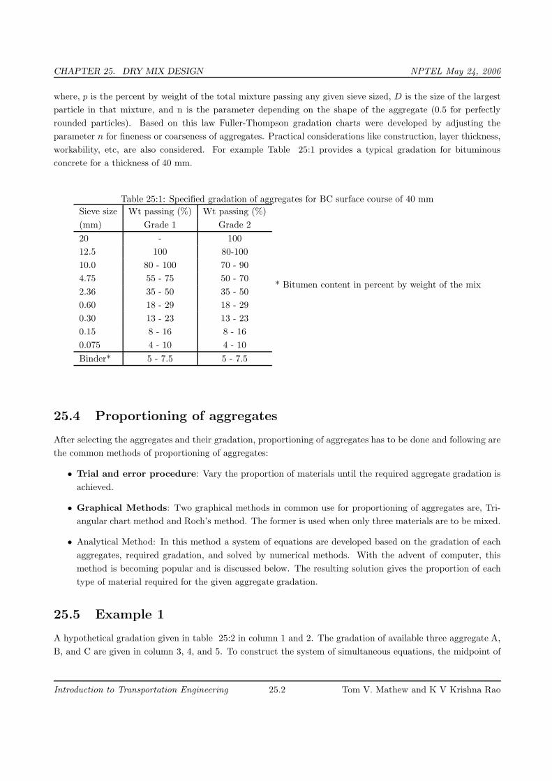
CHAPTER 25. DRY MIX DESIGN NPTEL May 24, 2006
where, p is the percent by weight of the total mixture passing any given sieve sized, D is the size of the largest
particle in that mixture, and n is the parameter depending on the shape of the aggregate (0.5 for perfectly
rounded particles). Based on this law Fuller-Thompson gradation charts were developed by adjusting the
parameter n for fineness or coarseness of aggregates. Practical considerations like construction, layer thickness,
workability, etc, are also considered. For example Table 25:1 provides a typical gradation for bituminous
concrete for a thickness of 40 mm.
Table 25:1: Specified gradation of aggregates for BC surface course of 40 mm
Sieve size Wt passing (%) Wt passing (%)
(mm) Grade 1 Grade 2
20 - 100
12.5 100 80-100
10.0 80 - 100 70 - 90
4.75 55 - 75 50 - 70
2.36 35 - 50 35 - 50
0.60 18 - 29 18 - 29
0.30 13 - 23 13 - 23
0.15 8 - 16 8 - 16
0.075 4 - 10 4 - 10
Binder* 5 - 7.5 5 - 7.5
* Bitumen content in percent by weight of the mix
25.4 Proportioning of aggregates
After selecting the aggregates and their gradation, proportioning of aggregates has to be done and following are
the common methods of proportioning of aggregates:
• Trial and error procedure: Vary the proportion of materials until the required aggregate gradation is
achieved.
• Graphical Methods: Two graphical methods in common use for proportioning of aggregates are, Tri-
angular chart method and Roch’s method. The former is used when only three materials are to be mixed.
• Analytical Method: In this method a system of equations are developed based on the gradation of each
aggregates, required gradation, and solved by numerical methods. With the advent of computer, this
method is becoming popular and is discussed below. The resulting solution gives the proportion of each
type of material required for the given aggregate gradation.
25.5 Example 1
A hypothetical gradation given in table 25:2 in column 1 and 2. The gradation of available three aggregate A,
B, and C are given in column 3, 4, and 5. To construct the system of simultaneous equations, the midpoint of
Introduction to Transportation Engineering 25.2 Tom V. Mathew and K V Krishna Rao
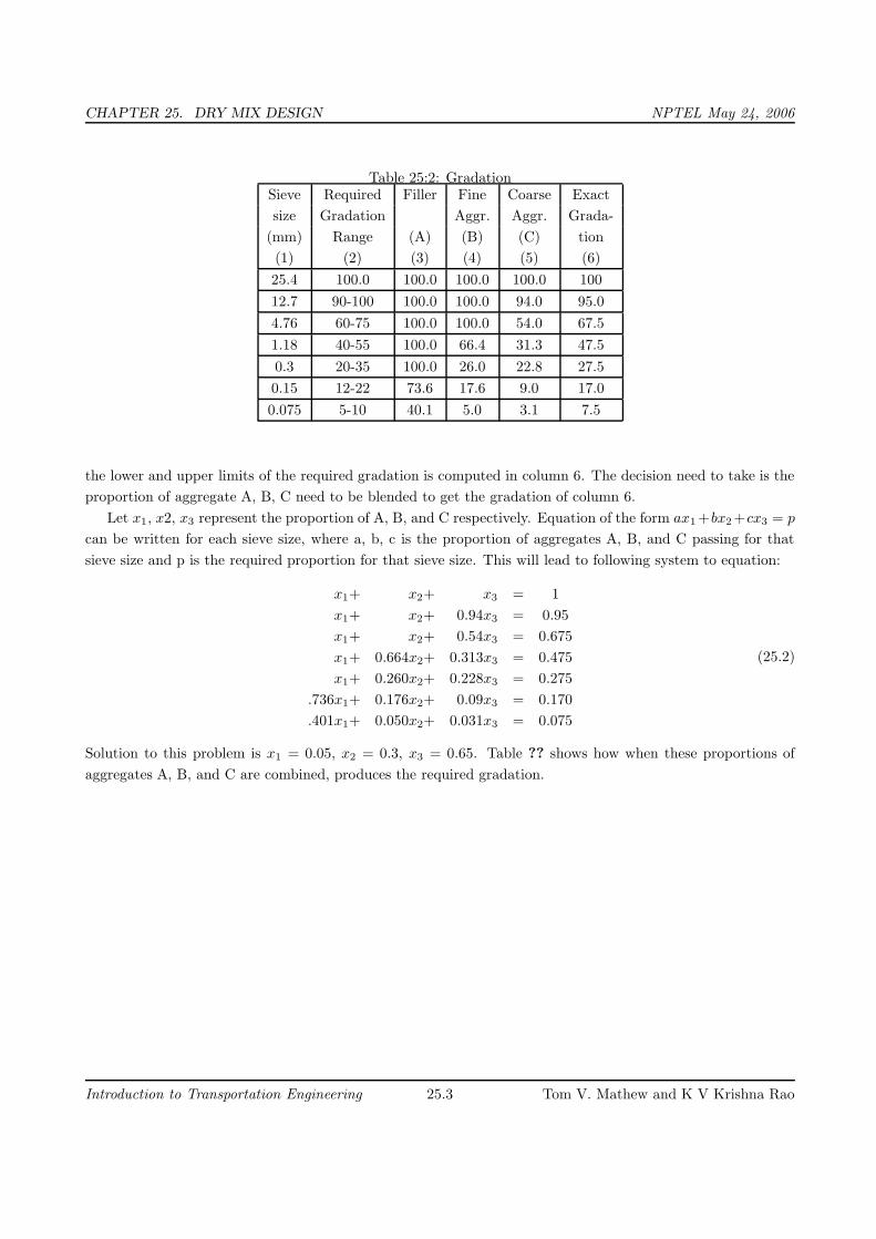
CHAPTER 25. DRY MIX DESIGN NPTEL May 24, 2006
Table 25:2: GradationSieve Required Filler Fine Coarse Exact
size Gradation Aggr. Aggr. Grada-
(mm) Range (A) (B) (C) tion
(1) (2) (3) (4) (5) (6)
25.4 100.0 100.0 100.0 100.0 100
12.7 90-100 100.0 100.0 94.0 95.0
4.76 60-75 100.0 100.0 54.0 67.5
1.18 40-55 100.0 66.4 31.3 47.5
0.3 20-35 100.0 26.0 22.8 27.5
0.15 12-22 73.6 17.6 9.0 17.0
0.075 5-10 40.1 5.0 3.1 7.5
the lower and upper limits of the required gradation is computed in column 6. The decision need to take is the
proportion of aggregate A, B, C need to be blended to get the gradation of column 6.
Let x1, x2, x3 represent the proportion of A, B, and C respectively. Equation of the form ax1 +bx2 +cx3 = p
can be written for each sieve size, where a, b, c is the proportion of aggregates A, B, and C passing for that
sieve size and p is the required proportion for that sieve size. This will lead to following system to equation:
x1+ x2+ x3 = 1
x1+ x2+ 0.94x3 = 0.95
x1+ x2+ 0.54x3 = 0.675
x1+ 0.664x2+ 0.313x3 = 0.475
x1+ 0.260x2+ 0.228x3 = 0.275
.736x1+ 0.176x2+ 0.09x3 = 0.170
.401x1+ 0.050x2+ 0.031x3 = 0.075
(25.2)
Solution to this problem is x1 = 0.05, x2 = 0.3, x3 = 0.65. Table ?? shows how when these proportions of
aggregates A, B, and C are combined, produces the required gradation.
Introduction to Transportation Engineering 25.3 Tom V. Mathew and K V Krishna Rao
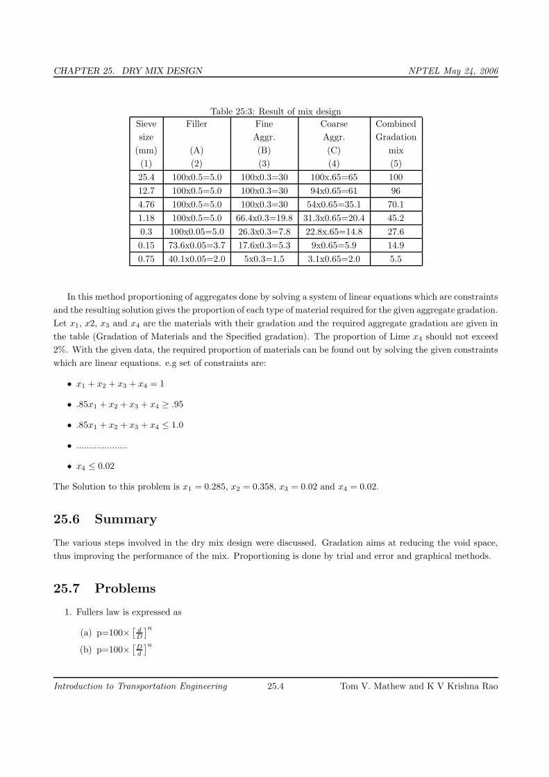
CHAPTER 25. DRY MIX DESIGN NPTEL May 24, 2006
Table 25:3: Result of mix design
Sieve Filler Fine Coarse Combined
size Aggr. Aggr. Gradation
(mm) (A) (B) (C) mix
(1) (2) (3) (4) (5)
25.4 100x0.5=5.0 100x0.3=30 100x.65=65 100
12.7 100x0.5=5.0 100x0.3=30 94x0.65=61 96
4.76 100x0.5=5.0 100x0.3=30 54x0.65=35.1 70.1
1.18 100x0.5=5.0 66.4x0.3=19.8 31.3x0.65=20.4 45.2
0.3 100x0.05=5.0 26.3x0.3=7.8 22.8x.65=14.8 27.6
0.15 73.6x0.05=3.7 17.6x0.3=5.3 9x0.65=5.9 14.9
0.75 40.1x0.05=2.0 5x0.3=1.5 3.1x0.65=2.0 5.5
In this method proportioning of aggregates done by solving a system of linear equations which are constraints
and the resulting solution gives the proportion of each type of material required for the given aggregate gradation.
Let x1, x2, x3 and x4 are the materials with their gradation and the required aggregate gradation are given in
the table (Gradation of Materials and the Specified gradation). The proportion of Lime x4 should not exceed
2%. With the given data, the required proportion of materials can be found out by solving the given constraints
which are linear equations. e.g set of constraints are:
• x1 + x2 + x3 + x4 = 1
• .85x1 + x2 + x3 + x4 ≥ .95
• .85x1 + x2 + x3 + x4 ≤ 1.0
• ....................
• x4 ≤ 0.02
The Solution to this problem is x1 = 0.285, x2 = 0.358, x3 = 0.02 and x4 = 0.02.
25.6 Summary
The various steps involved in the dry mix design were discussed. Gradation aims at reducing the void space,
thus improving the performance of the mix. Proportioning is done by trial and error and graphical methods.
25.7 Problems
1. Fullers law is expressed as
(a) p=100×[
d
D
]n
(b) p=100×[
D
d
]n
Introduction to Transportation Engineering 25.4 Tom V. Mathew and K V Krishna Rao
CHAPTER 25. DRY MIX DESIGN NPTEL May 24, 2006
Table 25:4: Gradation of Materials and the Specified gradation
Size Gradation of A Gradation of B Gradation of C Gradation of D Lower limit Upper limit
26.5 mm 100 100 100 100 100 100
22.4 mm 85.08 100 100 100 95 100
11.2 mm 1.48 80.68 100 100 55 75
5.6 mm 0 17.72 100 100 40 60
2.8 mm 0 0 85.13 100 30 45
710 m 0 0 59.61 15 100 22
355 m 0 0 37.45 10 100 18
180 m 0 0 24.96 8 100 15
90 m 0 0 15.85 0 100 8
(c) p=100×[
d2
D
]n
(d) p=100×[
d
D2
]n
25.8 Solutions
1. Fullers law is expressed as
(a) p=100×[
d
D
]n√
(b) p=100×[
D
d
]n
(c) p=100×[
d2
D
]n
(d) p=100×[
d
D2
]n
-
Introduction to Transportation Engineering 25.5 Tom V. Mathew and K V Krishna Rao
CHAPTER 27. FLEXIBLE PAVEMENT DESIGN NPTEL May 24, 2006
Chapter 27
Flexible pavement design
27.1 Overview
Flexible pavements are so named because the total pavement structure deflects, or flexes, under loading. A
flexible pavement structure is typically composed of several layers of materials. Each layer receives loads from
the above layer, spreads them out, and passes on these loads to the next layer below. Thus the stresses will be
reduced, which are maximum at the top layer and minimum on the top of subgrade. In order to take maximum
advantage of this property, layers are usually arranged in the order of descending load bearing capacity with the
highest load bearing capacity material (and most expensive) on the top and the lowest load bearing capacity
material (and least expensive) on the bottom.
27.2 Design procedures
For flexible pavements, structural design is mainly concerned with determining appropriate layer thickness and
composition. The main design factors are stresses due to traffic load and temperature variations. Two methods
of flexible pavement structural design are common today: Empirical design and mechanistic empirical design.
27.2.1 Empirical design
An empirical approach is one which is based on the results of experimentation or experience. Some of them are
either based on physical properties or strength parameters of soil subgrade. An empirical approach is one which
is based on the results of experimentation or experience. An empirical analysis of flexible pavement design can
be done with or with out a soil strength test. An example of design without soil strength test is by using is HRB
soil classification system, in which soils are grouped from A-1 to A-7 and a group index is added to differentiate
soils within each group. Example with soil strength test uses McLeod, Stabilometer, California Bearing Ratio
(CBR) test. CBR test is widely known and will be discussed.
27.2.2 Mechanistic-Empirical Design
Empirical-Mechanistic method of design is based on the mechanics of materials that relates input, such as
wheel load, to an output or pavement response. In pavement design, the responses are the stresses, strains,
and deflections within a pavement structure and the physical causes are the loads and material properties of
the pavement structure. The relationship between these phenomena and their physical causes are typically
described using some mathematical models. Along with this mechanistic approach, empirical elements are used
Introduction to Transportation Engineering 27.1 Tom V. Mathew and K V Krishna Rao
CHAPTER 27. FLEXIBLE PAVEMENT DESIGN NPTEL May 24, 2006
when defining what value of the calculated stresses, strains, and deflections result in pavement failure. The
relationship between physical phenomena and pavement failure is described by empirically derived equations
that compute the number of loading cycles to failure.
27.3 Traffic and Loading
There are three different approaches for considering vehicular and traffic characteristics, which affects pavement
design.
Fixed traffic: Thickness of pavement is governed by single load and number of load repetitions is not
considered. The heaviest wheel load anticipated is used for design purpose. This is an old method and is rarely
used today for pavement design.
Fixed vehicle: In the fixed vehicle procedure, the thickness is governed by the number of repetitions of a
standard axle load. If the axle load is not a standard one, then it must be converted to an equivalent axle load
by number of repetitions of given axle load and its equivalent axle load factor.
Variable traffic and vehicle: In this approach, both traffic and vehicle are considered individually, so
there is no need to assign an equivalent factor for each axle load. The loads can be divided in to a number of
groups and the stresses, strains, and deflections under each load group can be determined separately; and used
for design purposes. The traffic and loading factors to be considered include axle loads, load repetitions, and
tyre contact area.
27.3.1 Equivalent single wheel load
To carry maximum load with in the specified limit and to carry greater load, dual wheel, or dual tandem assembly
is often used. Equivalent single wheel load (ESWL) is the single wheel load having the same contact pressure,
which produces same value of maximum stress, deflection, tensile stress or contact pressure at the desired depth.
The procedure of finding the ESWL for equal stress criteria is provided below. This is a semi-rational method,
known as Boyd and Foster method, based on the following assumptions:
• equalancy concept is based on equal stress;
• contact area is circular;
• influence angle is 45o; and
• soil medium is elastic, homogeneous, and isotropic half space.
The ESWL is given by:
log10
ESWL = log10
P +0.301 log
10( z
d/2)
log10
( 2S
d/2)
(27.1)
where P is the wheel load, S is the center to center distance between the two wheels, d is the clear distance
between two wheels, and z is the desired depth.
Example 1
Find ESWL at depths of 5cm, 20cm and 40cm for a dual wheel carrying 2044 kg each. The center to center
tyre spacing is 20cm and distance between the walls of the two tyres is 10cm.
Introduction to Transportation Engineering 27.2 Tom V. Mathew and K V Krishna Rao
CHAPTER 27. FLEXIBLE PAVEMENT DESIGN NPTEL May 24, 2006
$(\log_{10}{ESWL}=\log_{10}P+\frac{0.301\log_{10}{(\frac{z}{d/2})}}{\log_{10}(\frac{2S}{d/2})})$
No stress overlap(ESWL=P)
No stress overlap
Partial stress overlap
Complete stress overlap (ESWL=2P)
z2s
d/2
P P
sd2a 2a
Figure 27:1: ESWL-Equal stress concept
Solution For desired depth z=40cm, which is twice the tyre spacing, ESWL = 2P=2×2044 = 4088 kN.
For z=5cm, which is half the distance between the walls of the tyre, ESWL = P = 2044kN. For z=20cm,
log10
ESWL = log10
P +0.301 log
10(
z
d/2)
log10
(2S
d/2)
=log10
ESWL = log10
2044+0.301 log
10(
20
10/2)
log10
(2×20
10/2)
=3.511. Therefore, ESWL
= antilog(3.511)= 3244.49 kN
27.3.2 Equivalent single axle load
Vehicles can have many axles which will distribute the load into different axles, and in turn to the pavement
through the wheels. A standard truck has two axles, front axle with two wheels and rear axle with four wheels.
But to carry large loads multiple axles are provided. Since the design of flexible pavements is by layered theory,
only the wheels on one side needed to be considered. On the other hand, the design of rigid pavement is by plate
theory and hence the wheel load on both sides of axle need to be considered. Legal axle load: The maximum
allowed axle load on the roads is called legal axle load. For highways the maximum legal axle load in India,
specified by IRC, is 10 tonnes. Standard axle load: It is a single axle load with dual wheel carrying 80 KN load
and the design of pavement is based on the standard axle load.
Repetition of axle loads: The deformation of pavement due to a single application of axle load may
be small but due to repeated application of load there would be accumulation of unrecovered or permanent
deformation which results in failure of pavement. If the pavement structure fails with N1 number of repetition
of load W1 and for the same failure criteria if it requires N2 number of repetition of load W2, then W1N1
and W2N2 are considered equivalent. Note that, W1N1 and W2N2 equivalency depends on the failure criterion
employed.
Equivalent axle load factor: An equivalent axle load factor (EALF) defines the damage per pass to a pavement
by the ith type of axle relative to the damage per pass of a standard axle load. While finding the EALF, the
failure criterion is important. Two types of failure criterias are commonly adopted: fatigue cracking and ruttings.
The fatigue cracking model has the following form:
Nf = f1 (εt)−f2 × (E)−f3 orNf ∝ εt
−f2 (27.2)
where, Nf is the number of load repetition for a certain percentage of cracking, εt is the tensile strain at the
bottom of the binder course, E is the modulus of elasticity, and f1, f2, f3 are constants. If we consider fatigue
Introduction to Transportation Engineering 27.3 Tom V. Mathew and K V Krishna Rao
CHAPTER 27. FLEXIBLE PAVEMENT DESIGN NPTEL May 24, 2006
cracking as failure criteria, and a typical value of 4 for f2, then:
EALF =
(
εi
εstd
)4
(27.3)
where, i indicate ith vehicle, and std indicate the standard axle. Now if we assume that the strain is proportional
to the wheel load,
EALF =
(
Wi
Wstd
)4
(27.4)
Similar results can be obtained if rutting model is used, which is:
Nd = f4 (εc)−f5 (27.5)
where Nd is the permissible design rut depth (say 20mm), εc is the compressive strain at the top of the subgrade,
and f4, f5 are constants. Once we have the EALF, then we can get the ESAL as given below.
Equivalent single axle load, ESAL =m
∑
i=1
Fini (27.6)
where,m is the number of axle load groups, Fi is the EALF for ith axle load group, and ni is the number of
passes of ith axle load group during the design period.
Example Let number of load repetition expected by 80 KN standard axle is 1000, 160 KN is 100 and 40 KN
is 10000. Find the equivalent axle load. Solution:
Table 27:1: Example Solution
Axle No.of Load EALF
Load Repetition
i (KN) (ni) (Fi) Fini
1 40 10000 (40/80)4 = 0.0625 625
2 80 1000 (80/80)4 = 1 1000
3 160 100 (160/80)4
= 16 1600
ESAL=∑
Fini = 3225 kN
27.3.3 Example2
Let the number of load repetition expected by 120 kN axle is 1000, 160 kN is 100, and 40 kN is 10,000. Find
the equivalent standard axle load if the equivalence criteria is rutting. Assume 80 kN as standard axle load and
the rutting model is Nr = f4ε−f5
cwhere f4 =4.2 and f5 =4.5.
Solution
ESAL=∑
Fini = 8904.94 kN
Introduction to Transportation Engineering 27.4 Tom V. Mathew and K V Krishna Rao
CHAPTER 27. FLEXIBLE PAVEMENT DESIGN NPTEL May 24, 2006
Table 27:2: Example Solution
Axle No.of Load EALF
Load Repetition
i (KN) (ni) (Fi) Fini
1 120 1000 (120/80)4
= 6.200 6200
2 160 100 (160/80)4
= 22.63 2263
3 40 10000 (40/80)4 = 0.04419 441.9
27.3.4 Example
Let number of load repetition expected by 60kN standard axle is 1000, 120kN is 200 and 40 kN is 10000.
Find the equivalent axle load using fatigue cracking as failure criteria according to IRC. Hint:Nf = 2.21 ×
10−4(εt)−3.89(E)0.854
Solution
Table 27:3: Example Solution
Axle No.of Load EALF
Load Repetition
i (KN) (ni) (Fi) Fini
1 40 10000 (40/60)3 .89 = 0.2065 2065
2 60 1000 (60/60)3 .89 = 1 1000
3 120 200 (120/60)3.89 = 14.825 2965.081
ESAL=∑
Fini = 6030.81 kN
27.4 Material characterization
It is well known that the pavement materials are not perfectly elastic but experiences some permanent deforma-
tion after each load repetitions. It is well known that most paving materials are not elastic but experience some
permanent deformation after each load application. However, if the load is small compared to the strength of
the material and is repeated for a large number of times, the deformation under each load repetition is nearly
completely recoverable and proportional to the load and can be considered as elastic.
The Figure 27:2 shows straining of a specimen under a repeated load test. At the initial stage of load
applications, there is considerable permanent deformation as indicated by the plastic strain in the Figure 27:2.
As the number of repetition increases, the plastic strain due to each load repetition decreases. After 100 to 200
repetitions, the strain is practically all-recoverable, as indicated by εr in the figure.
27.4.1 Resilient modulus of soil
The elastic modulus based on the recoverable strain under repeated loads is called the resilient modulus MR,
defined as MR = σd
εr
. In which σd is the deviator stress, which is the axial stress in an unconfined compression
test or the axial stress in excess of the confining pressure in a triaxial compression test.
Introduction to Transportation Engineering 27.5 Tom V. Mathew and K V Krishna Rao
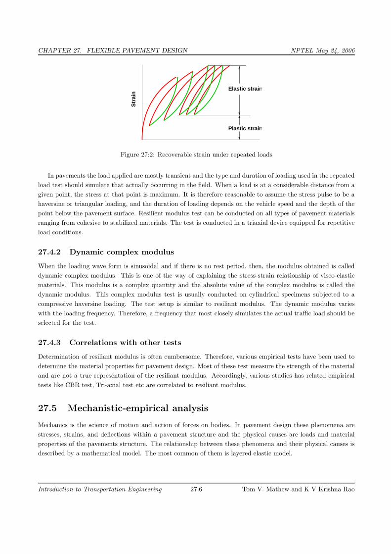
CHAPTER 27. FLEXIBLE PAVEMENT DESIGN NPTEL May 24, 2006
Str
ain
Elastic strain
Plastic strain
Figure 27:2: Recoverable strain under repeated loads
In pavements the load applied are mostly transient and the type and duration of loading used in the repeated
load test should simulate that actually occurring in the field. When a load is at a considerable distance from a
given point, the stress at that point is maximum. It is therefore reasonable to assume the stress pulse to be a
haversine or triangular loading, and the duration of loading depends on the vehicle speed and the depth of the
point below the pavement surface. Resilient modulus test can be conducted on all types of pavement materials
ranging from cohesive to stabilized materials. The test is conducted in a triaxial device equipped for repetitive
load conditions.
27.4.2 Dynamic complex modulus
When the loading wave form is sinusoidal and if there is no rest period, then, the modulus obtained is called
dynamic complex modulus. This is one of the way of explaining the stress-strain relationship of visco-elastic
materials. This modulus is a complex quantity and the absolute value of the complex modulus is called the
dynamic modulus. This complex modulus test is usually conducted on cylindrical specimens subjected to a
compressive haversine loading. The test setup is similar to resiliant modulus. The dynamic modulus varies
with the loading frequency. Therefore, a frequency that most closely simulates the actual traffic load should be
selected for the test.
27.4.3 Correlations with other tests
Determination of resiliant modulus is often cumbersome. Therefore, various empirical tests have been used to
determine the material properties for pavement design. Most of these test measure the strength of the material
and are not a true representation of the resiliant modulus. Accordingly, various studies has related empirical
tests like CBR test, Tri-axial test etc are correlated to resiliant modulus.
27.5 Mechanistic-empirical analysis
Mechanics is the science of motion and action of forces on bodies. In pavement design these phenomena are
stresses, strains, and deflections within a pavement structure and the physical causes are loads and material
properties of the pavements structure. The relationship between these phenomena and their physical causes is
described by a mathematical model. The most common of them is layered elastic model.
Introduction to Transportation Engineering 27.6 Tom V. Mathew and K V Krishna Rao
CHAPTER 27. FLEXIBLE PAVEMENT DESIGN NPTEL May 24, 2006
27.5.1 Advantages
The basic advantages of the Mechanistic-Empirical pavement design method over a purely empirical one are:
1. It can be used for both existing pavement rehabilitation and new pavement construction
2. It can accommodate changing load types
3. It can better characterize materials allowing for
• better utilization of available materials
• accommodation of new materials
• improved definition of existing layer proportion
4. It uses material proportion that relates better with actual pavement performance
5. It provides more reliable performance predictions
6. It defines role of construction in a better way
7. It accommodates environment and aging effect of materials in the pavement
27.5.2 Mechanistic model
Mechanistic models are used to mathematically model pavement physics. There are a number of different types
of models available today (e.g., layered elastic, dynamic, viscoelastic) but this section will present the layered
elastic model.
Layered elastic model
A layered elastic model can compute stresses, strains and deflections at any point in a pavement structure
resulting from the application of a surface load. Layered elastic models assume that each pavement structural
layer is homogeneous, isotropic, and linearly elastic. In other words, it is the same everywhere and will rebound
to its original form once the load is removed. This section covers the basic assumptions, inputs and outputs
from a typical layered elastic model.
Assumptions in layered elastic model
The layered elastic approach works with relatively simple mathematical models and thus requires following
assumptions
• Pavement layer extends infinitely in the horizontal direction
• The bottom layer (usually the subgrade) extends infinitely downwards
• Materials are not stressed beyond their elastic ranges
Introduction to Transportation Engineering 27.7 Tom V. Mathew and K V Krishna Rao
CHAPTER 27. FLEXIBLE PAVEMENT DESIGN NPTEL May 24, 2006
Inputs
A layered elastic model requires a minimum number of inputs to adequately characterize a pavement structure
and its response to loading. These inputs are:
• Material properties of each layer, like modulus of elasticity (E), Poisson’s ratio (ν),
• Pavement layer thicknesses, and
• Loading conditions which include the total wheel load (P ) and load repetitions.
Output
The outputs of the layered elastic model are the stresses, strains and deflections in the pavements.
• Stress. The intensity of internally distributed forces experienced within the pavement structure at various
points. Stress has units of force per unit area(pa)
• Strain. The unit displacement due to stress , usually expressed as a ratio of change in dimension to the
original dimension (mm/mm )
• Deflection. The linear change in dimension. Deflection is expressed in units of length (mm)
Failure criteria
The main empirical portions of the mechanistic-empirical design process are the equations used to compute the
number of loading cycles to failure. These equations are derived by observing the performance of pavements
and relating the type and extent of observed failure to an initial strain under various loads. Currently, two
types of failure criteria are widely recognized, one relating to fatigue cracking and the other to rutting initiating
in the subgrade.
27.6 Summary
Basic concepts of flexible pavement design were discussed. There are two main design procedures- empirical
and mechanistic empirical design. For design purposes, equivalent single wheel load and equivalent single axle
load concepts are used.
27.7 Problems
1. A set of dual tyres has a total load of 4090 kg, a contact radius a of 11.4 cm and a center to center tyre
spacing of 34.3 cm. Find the ESWL by Boyd & Foster method for a depth of 34.3 cm. [Ans: 3369.3 kg]
2. Calculate ESWL by equal stress criteria for a dual wheel assembly carrying 2044 kg each for a pavement
thickness of 5, 15, 20, 25 and 30 cms. The distance between walls of the tyre is 11 cm. Use either graphical
or functional methods. (Hint: P=2044kg, d=11cm, s=27cm). [Ans: 2044, 2760, 3000, 3230 and 4088]
3. Let number of load repetition expected by 60kN standard axle is 1000, 120kN is 200 and 40 kN is 10000.
Find the equivalent axle load using fatigue cracking as failure criteria according to IRC. Hint:Nf =
2.21× 10⁻⁴(εt)−3.89(E)0.854
Introduction to Transportation Engineering 27.8 Tom V. Mathew and K V Krishna Rao
CHAPTER 28. IRC METHOD OF DESIGN OF FLEXIBLE PAVEMENTS NPTEL May 24, 2006
Chapter 28
IRC method of design of flexible
pavements
28.1 Overview
Indian roads congress has specified the design procedures for flexible pavements based on CBR values. The
Pavement designs given in the previous edition IRC:37-1984 were applicable to design traffic upto only 30 million
standard axles (msa). The earlier code is empirical in nature which has limitations regarding applicability and
extrapolation. This guidelines follows analytical designs and developed new set of designs up to 150 msa.
28.2 Scope
These guidelines will apply to design of flexible pavements for Expressway, National Highways, State Highways,
Major District Roads, and other categories of roads. Flexible pavements are considered to include the pavements
which have bituminous surfacing and granular base and sub-base courses conforming to IRC/ MOST standards.
These guidelines apply to new pavements.
28.3 Design criteria
The flexible pavements has been modeled as a three layer structure and stresses and strains at critical locations
have been computed using the linear elastic model. To give proper consideration to the aspects of performance,
the following three types of pavement distress resulting from repeated (cyclic) application of traffic loads are
considered:
1. vertical compressive strain at the top of the sub-grade which can cause sub-grade deformation resulting
in permanent deformation at the pavement surface.
2. horizontal tensile strain or stress at the bottom of the bituminous layer which can cause fracture of the
bituminous layer.
3. pavement deformation within the bituminous layer.
While the permanent deformation within the bituminous layer can be controlled by meeting the mix design
requirements, thickness of granular and bituminous layers are selected using the analytical design approach so
that strains at the critical points are within the allowable limits. For calculating tensile strains at the bottom
Introduction to Transportation Engineering 28.1 Tom V. Mathew and K V Krishna Rao
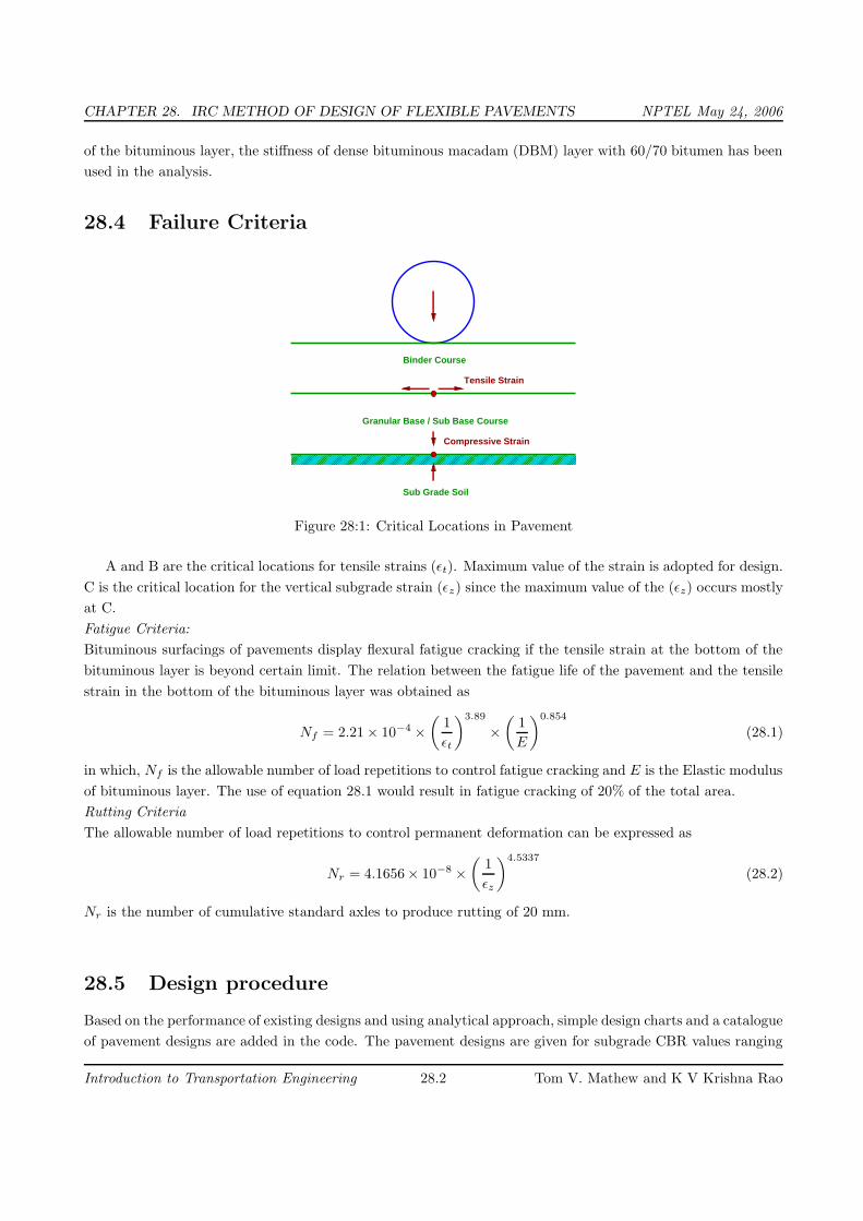
CHAPTER 28. IRC METHOD OF DESIGN OF FLEXIBLE PAVEMENTS NPTEL May 24, 2006
of the bituminous layer, the stiffness of dense bituminous macadam (DBM) layer with 60/70 bitumen has been
used in the analysis.
28.4 Failure Criteria
������������������������������������������������������������������������������������������������������������������������������������������������������������������������������������������������������������������������������������������������������������������������������������������������
Compressive Strain
Tensile Strain
Sub Grade Soil
Granular Base / Sub Base Course
Binder Course
Figure 28:1: Critical Locations in Pavement
A and B are the critical locations for tensile strains (εt). Maximum value of the strain is adopted for design.
C is the critical location for the vertical subgrade strain (εz) since the maximum value of the (εz) occurs mostly
at C.
Fatigue Criteria:
Bituminous surfacings of pavements display flexural fatigue cracking if the tensile strain at the bottom of the
bituminous layer is beyond certain limit. The relation between the fatigue life of the pavement and the tensile
strain in the bottom of the bituminous layer was obtained as
Nf = 2.21× 10⁻⁴ ×
(
1
εt
)3.89
×
(
1
E
)0.854
(28.1)
in which, Nf is the allowable number of load repetitions to control fatigue cracking and E is the Elastic modulus
of bituminous layer. The use of equation 28.1 would result in fatigue cracking of 20% of the total area.
Rutting Criteria
The allowable number of load repetitions to control permanent deformation can be expressed as
Nr = 4.1656× 10⁻⁸ ×
(
1
εz
)4.5337
(28.2)
Nr is the number of cumulative standard axles to produce rutting of 20 mm.
28.5 Design procedure
Based on the performance of existing designs and using analytical approach, simple design charts and a catalogue
of pavement designs are added in the code. The pavement designs are given for subgrade CBR values ranging
Introduction to Transportation Engineering 28.2 Tom V. Mathew and K V Krishna Rao
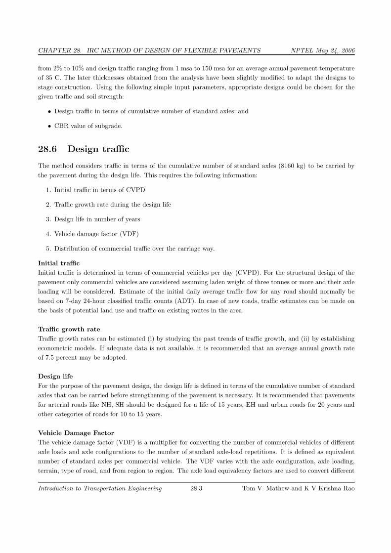
CHAPTER 28. IRC METHOD OF DESIGN OF FLEXIBLE PAVEMENTS NPTEL May 24, 2006
from 2% to 10% and design traffic ranging from 1 msa to 150 msa for an average annual pavement temperature
of 35 C. The later thicknesses obtained from the analysis have been slightly modified to adapt the designs to
stage construction. Using the following simple input parameters, appropriate designs could be chosen for the
given traffic and soil strength:
• Design traffic in terms of cumulative number of standard axles; and
• CBR value of subgrade.
28.6 Design traffic
The method considers traffic in terms of the cumulative number of standard axles (8160 kg) to be carried by
the pavement during the design life. This requires the following information:
1. Initial traffic in terms of CVPD
2. Traffic growth rate during the design life
3. Design life in number of years
4. Vehicle damage factor (VDF)
5. Distribution of commercial traffic over the carriage way.
Initial traffic
Initial traffic is determined in terms of commercial vehicles per day (CVPD). For the structural design of the
pavement only commercial vehicles are considered assuming laden weight of three tonnes or more and their axle
loading will be considered. Estimate of the initial daily average traffic flow for any road should normally be
based on 7-day 24-hour classified traffic counts (ADT). In case of new roads, traffic estimates can be made on
the basis of potential land use and traffic on existing routes in the area.
Traffic growth rate
Traffic growth rates can be estimated (i) by studying the past trends of traffic growth, and (ii) by establishing
econometric models. If adequate data is not available, it is recommended that an average annual growth rate
of 7.5 percent may be adopted.
Design life
For the purpose of the pavement design, the design life is defined in terms of the cumulative number of standard
axles that can be carried before strengthening of the pavement is necessary. It is recommended that pavements
for arterial roads like NH, SH should be designed for a life of 15 years, EH and urban roads for 20 years and
other categories of roads for 10 to 15 years.
Vehicle Damage Factor
The vehicle damage factor (VDF) is a multiplier for converting the number of commercial vehicles of different
axle loads and axle configurations to the number of standard axle-load repetitions. It is defined as equivalent
number of standard axles per commercial vehicle. The VDF varies with the axle configuration, axle loading,
terrain, type of road, and from region to region. The axle load equivalency factors are used to convert different
Introduction to Transportation Engineering 28.3 Tom V. Mathew and K V Krishna Rao
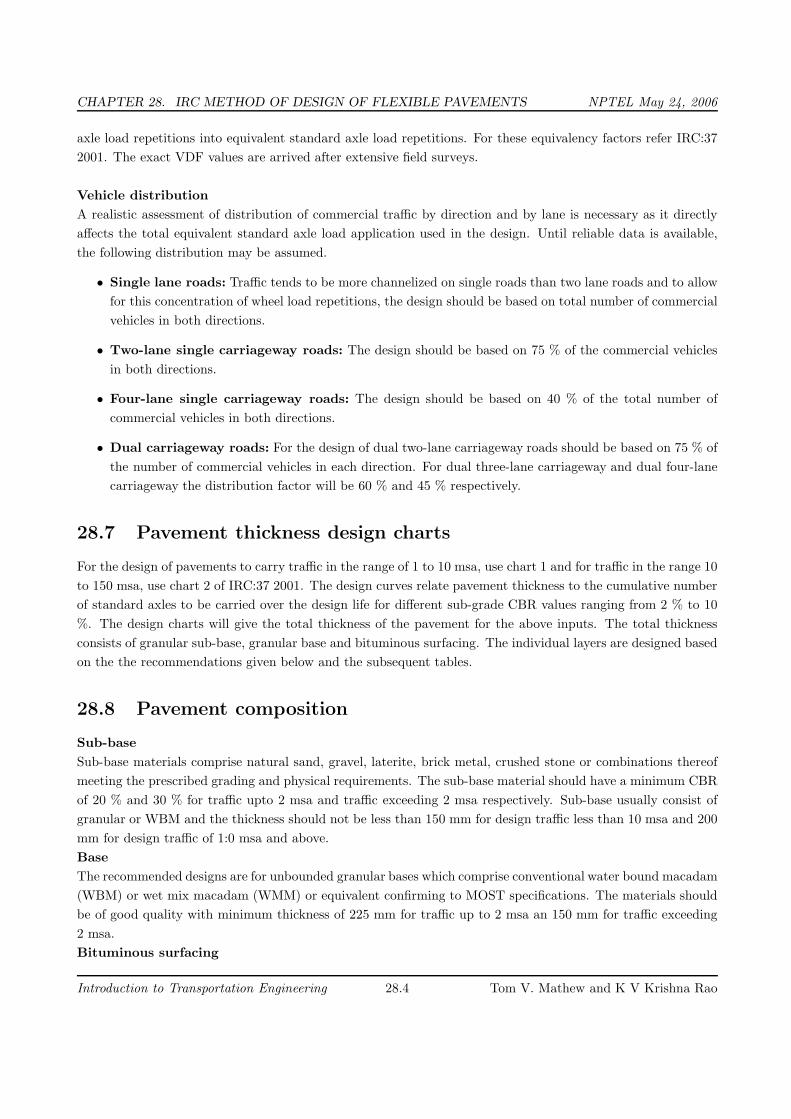
CHAPTER 28. IRC METHOD OF DESIGN OF FLEXIBLE PAVEMENTS NPTEL May 24, 2006
axle load repetitions into equivalent standard axle load repetitions. For these equivalency factors refer IRC:37
2001. The exact VDF values are arrived after extensive field surveys.
Vehicle distribution
A realistic assessment of distribution of commercial traffic by direction and by lane is necessary as it directly
affects the total equivalent standard axle load application used in the design. Until reliable data is available,
the following distribution may be assumed.
• Single lane roads: Traffic tends to be more channelized on single roads than two lane roads and to allow
for this concentration of wheel load repetitions, the design should be based on total number of commercial
vehicles in both directions.
• Two-lane single carriageway roads: The design should be based on 75 % of the commercial vehicles
in both directions.
• Four-lane single carriageway roads: The design should be based on 40 % of the total number of
commercial vehicles in both directions.
• Dual carriageway roads: For the design of dual two-lane carriageway roads should be based on 75 % of
the number of commercial vehicles in each direction. For dual three-lane carriageway and dual four-lane
carriageway the distribution factor will be 60 % and 45 % respectively.
28.7 Pavement thickness design charts
For the design of pavements to carry traffic in the range of 1 to 10 msa, use chart 1 and for traffic in the range 10
to 150 msa, use chart 2 of IRC:37 2001. The design curves relate pavement thickness to the cumulative number
of standard axles to be carried over the design life for different sub-grade CBR values ranging from 2 % to 10
%. The design charts will give the total thickness of the pavement for the above inputs. The total thickness
consists of granular sub-base, granular base and bituminous surfacing. The individual layers are designed based
on the the recommendations given below and the subsequent tables.
28.8 Pavement composition
Sub-base
Sub-base materials comprise natural sand, gravel, laterite, brick metal, crushed stone or combinations thereof
meeting the prescribed grading and physical requirements. The sub-base material should have a minimum CBR
of 20 % and 30 % for traffic upto 2 msa and traffic exceeding 2 msa respectively. Sub-base usually consist of
granular or WBM and the thickness should not be less than 150 mm for design traffic less than 10 msa and 200
mm for design traffic of 1:0 msa and above.
Base
The recommended designs are for unbounded granular bases which comprise conventional water bound macadam
(WBM) or wet mix macadam (WMM) or equivalent confirming to MOST specifications. The materials should
be of good quality with minimum thickness of 225 mm for traffic up to 2 msa an 150 mm for traffic exceeding
2 msa.
Bituminous surfacing
Introduction to Transportation Engineering 28.4 Tom V. Mathew and K V Krishna Rao
CHAPTER 28. IRC METHOD OF DESIGN OF FLEXIBLE PAVEMENTS NPTEL May 24, 2006
The surfacing consists of a wearing course or a binder course plus wearing course. The most commonly used
wearing courses are surface dressing, open graded premix carpet, mix seal surfacing, semi-dense bituminous
concrete and bituminous concrete. For binder course, MOST specifies, it is desirable to use bituminous macadam
(BM) for traffic upto o 5 msa and dense bituminous macadam (DBM) for traffic more than 5 msa.
28.9 Numerical example
Design the pavement for construction of a new bypass with the following data:
1. Two lane carriage way
2. Initial traffic in the year of completion of construction = 400 CVPD (sum of both directions)
3. Traffic growth rate = 7.5 %
4. Design life = 15 years
5. Vehicle damage factor based on axle load survey = 2.5 standard axle per commercial vehicle
6. Design CBR of subgrade soil = 4%.
Solution
1. Distribution factor = 0.75
2.
N =365×
[
(1 + 0.075)15 − 1)]
0.075× 400× 0.75× 2.5
= 7200000
= 7.2 msa
3. Total pavement thickness for CBR 4% and traffic 7.2 msa from IRC:37 2001 chart1 = 660 mm
4. Pavement composition can be obtained by interpolation from Pavement Design Catalogue (IRC:37 2001).
(a) Bituminous surfacing = 25 mm SDBC + 70 mm DBM
(b) Road-base = 250 mm WBM
(c) sub-base = 315 mm granular material of CBR not less than 30 %
28.10 Summary
The design procedure given by IRC makes use of the CBR value, million standard axle concept, and vehicle
damage factor. Traffic distribution along the lanes are taken into account. The design is meant for design traffic
which is arrived at using a growth rate.
Introduction to Transportation Engineering 28.5 Tom V. Mathew and K V Krishna Rao
CHAPTER 28. IRC METHOD OF DESIGN OF FLEXIBLE PAVEMENTS NPTEL May 24, 2006
28.11 Problems
1. Design the pavement for construction of a new two lane carriageway for design life 15 years using IRC
method. The initial traffic in the year of completion in each direction is 150 CVPD and growth rate is
5%. Vehicle damage factor based on axle load survey = 2.5 std axle per commercial vehicle. Design CBR
of subgrade soil=4%.
28.12 Solutions
1. Distribution factor = 0.75
2.
N =365×
[
(1 + 0.05)15 − 1)]
0.05× 300× 0.75× 2.5
= 4430348.837
= 4.4 msa
3. Total pavement thickness for CBR 4% and traffic 4.4 msa from IRC:37 2001 chart1 = 580 mm
4. Pavement composition can be obtained by interpolation from Pavement Design Catalogue (IRC:37 2001).
(a) Bituminous surfacing = 20 mm PC + 50 mm BM
(b) Road-base = 250 mm Granular base
(c) sub-base = 280 mm granular material.
Introduction to Transportation Engineering 28.6 Tom V. Mathew and K V Krishna Rao
CHAPTER 29. RIGID PAVEMENT DESIGN NPTEL May 24, 2006
Chapter 29
Rigid pavement design
29.1 Overview
As the name implies, rigid pavements are rigid i.e, they do not flex much under loading like flexible pavements.
They are constructed using cement concrete. In this case, the load carrying capacity is mainly due to the
rigidity ad high modulus of elasticity of the slab (slab action). H. M. Westergaard is considered the pioneer in
providing the rational treatment of the rigid pavement analysis.
29.1.1 Modulus of sub-grade reaction
Westergaard considered the rigid pavement slab as a thin elastic plate resting on soil sub-grade, which is assumed
as a dense liquid. The upward reaction is assumed to be proportional to the deflection. Base on this assumption,
Westergaard defined a modulus of sub-grade reaction K in kg/cm3 given by K = p
∆where ∆ is the displacement
level taken as 0.125 cm and p is the pressure sustained by the rigid plate of 75 cm diameter at a deflection of
0.125 cm.
29.1.2 Relative stiffness of slab to sub-grade
A certain degree of resistance to slab deflection is offered by the sub-grade. The sub-grade deformation is
same as the slab deflection. Hence the slab deflection is direct measurement of the magnitude of the sub-grade
pressure. This pressure deformation characteristics of rigid pavement lead Westergaard to the define the term
radius of relative stiffness l in cm is given by the equation 29.1.
l = 4
√
Eh3
12K(1− µ2)(29.1)
where E is the modulus of elasticity of cement concrete in kg/cm2 (3.0×10⁵), µ is the Poisson’s ratio of concrete
(0.15), h is the slab thickness in cm and K is the modulus of sub-grade reaction.
29.1.3 Critical load positions
Since the pavement slab has finite length and width, either the character or the intensity of maximum stress
induced by the application of a given traffic load is dependent on the location of the load on the pavement
surface. There are three typical locations namely the interior, edge and corner, where differing conditions of
slab continuity exist. These locations are termed as critical load positions.
Introduction to Transportation Engineering 29.1 Tom V. Mathew and K V Krishna Rao
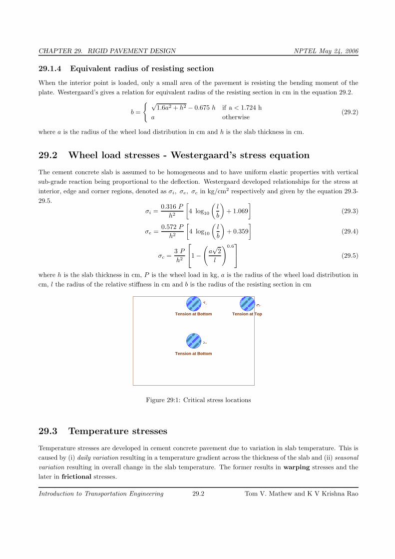
CHAPTER 29. RIGID PAVEMENT DESIGN NPTEL May 24, 2006
29.1.4 Equivalent radius of resisting section
When the interior point is loaded, only a small area of the pavement is resisting the bending moment of the
plate. Westergaard’s gives a relation for equivalent radius of the resisting section in cm in the equation 29.2.
b =
{ √1.6a2 + h2 − 0.675 h if a < 1.724 h
a otherwise(29.2)
where a is the radius of the wheel load distribution in cm and h is the slab thickness in cm.
29.2 Wheel load stresses - Westergaard’s stress equation
The cement concrete slab is assumed to be homogeneous and to have uniform elastic properties with vertical
sub-grade reaction being proportional to the deflection. Westergaard developed relationships for the stress at
interior, edge and corner regions, denoted as σi, σe, σc in kg/cm2 respectively and given by the equation 29.3-
29.5.
σi =0.316 P
h2
[
4 log10
(
l
b
)
+ 1.069
]
(29.3)
σe =0.572 P
h2
[
4 log10
(
l
b
)
+ 0.359
]
(29.4)
σc =3 P
h2
1 −
(
a√
2
l
)0.6
(29.5)
where h is the slab thickness in cm, P is the wheel load in kg, a is the radius of the wheel load distribution in
cm, l the radius of the relative stiffness in cm and b is the radius of the resisting section in cm
������������������������������������
������������������������������������
����������������������������
����������������������������
����������������������������
����������������������������
Tension at Bottom
Tension at Bottom Tension at Top
��
�
��
Figure 29:1: Critical stress locations
29.3 Temperature stresses
Temperature stresses are developed in cement concrete pavement due to variation in slab temperature. This is
caused by (i) daily variation resulting in a temperature gradient across the thickness of the slab and (ii) seasonal
variation resulting in overall change in the slab temperature. The former results in warping stresses and the
later in frictional stresses.
Introduction to Transportation Engineering 29.2 Tom V. Mathew and K V Krishna Rao
CHAPTER 29. RIGID PAVEMENT DESIGN NPTEL May 24, 2006
29.3.1 Warping stress
The warping stress at the interior, edge and corner regions, denoted as σti, σte
, σtcin kg/cm2 respectively and
given by the equation 29.7-29.8.
σti=
Eεt
2
(
Cx + µCy
1 − µ2
)
(29.6)
σte= Max
(
CxEεt
2,CyEεt
2
)
(29.7)
σtc=
Eεt
3(1 − µ)
√
a
l(29.8)
where E is the modulus of elasticity of concrete in kg/cm2 (3×10⁵), ε is the thermal coefficient of concrete
per oC (1×10⁻⁷) t is the temperature difference between the top and bottom of the slab, Cx and Cy are the
coefficient based on Lx/l in the desired direction and Ly/l right angle to the desired direction, µ is the Poisson’s
ration (0.15), a is the radius of the contact area and l is the radius of the relative stiffness.
29.3.2 Frictional stresses
The frictional stress σf in kg/cm2 is given by the equation
σf =WLf
2 × 10⁴(29.9)
where W is the unit weight of concrete in kg/cm2 (2400), f is the coefficient of sub grade friction (1.5) and L
is the length of the slab in meters.
29.4 Combination of stresses
The cumulative effect of the different stress give rise to the following thee critical cases
• Summer, mid-day: The critical stress is for edge region given by σcritical = σe + σte− σf
• Winter, mid-day: The critical combination of stress is for the edge region given by σcritical = σe +σte+σf
• Mid-nights: The critical combination of stress is for the corner region given by σcritical = σc + σtc
29.5 Design of joints
29.5.1 Expansion joints
The purpose of the expansion joint is to allow the expansion of the pavement due to rise in temperature with
respect to construction temperature. The design consideration are:
• Provided along the longitudinal direction,
• design involves finding the joint spacing for a given expansion joint thickness (say 2.5 cm specified by
IRC) subjected to some maximum spacing (say 140 as per IRC)
Introduction to Transportation Engineering 29.3 Tom V. Mathew and K V Krishna Rao
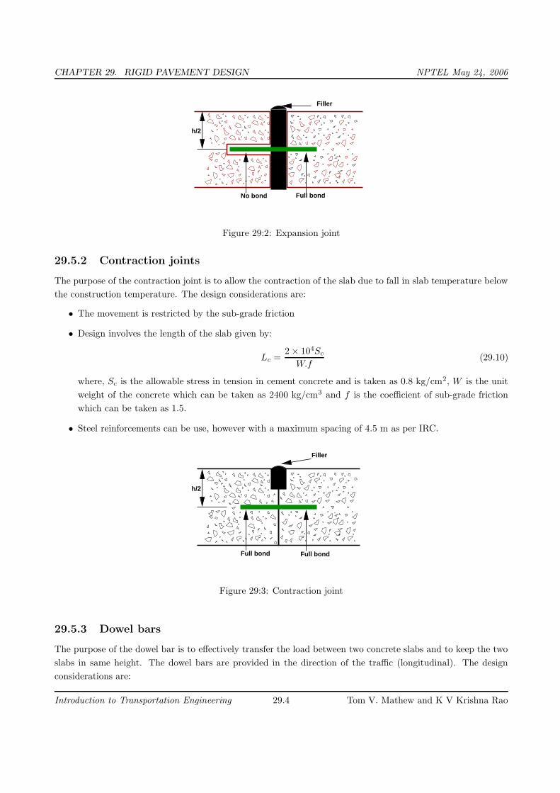
CHAPTER 29. RIGID PAVEMENT DESIGN NPTEL May 24, 2006
Full bondNo bond
h/2
Filler
Figure 29:2: Expansion joint
29.5.2 Contraction joints
The purpose of the contraction joint is to allow the contraction of the slab due to fall in slab temperature below
the construction temperature. The design considerations are:
• The movement is restricted by the sub-grade friction
• Design involves the length of the slab given by:
Lc =2 × 10⁴Sc
W.f(29.10)
where, Sc is the allowable stress in tension in cement concrete and is taken as 0.8 kg/cm2, W is the unit
weight of the concrete which can be taken as 2400 kg/cm3 and f is the coefficient of sub-grade friction
which can be taken as 1.5.
• Steel reinforcements can be use, however with a maximum spacing of 4.5 m as per IRC.
Full bondFull bond
h/2
Filler
Figure 29:3: Contraction joint
29.5.3 Dowel bars
The purpose of the dowel bar is to effectively transfer the load between two concrete slabs and to keep the two
slabs in same height. The dowel bars are provided in the direction of the traffic (longitudinal). The design
considerations are:
Introduction to Transportation Engineering 29.4 Tom V. Mathew and K V Krishna Rao
CHAPTER 29. RIGID PAVEMENT DESIGN NPTEL May 24, 2006
• Mild steel rounded bars,
• bonded on one side and free on other side
Bradbury’s analysis
Bradbury’s analysis gives load transfer capacity of single dowel bar in shear, bending and bearing as follows:
Ps = 0.785 d2 Fs (29.11)
Pf =2 d3 Ff
Ld + 8.8δ(29.12)
Pb =Fb L2
dd
12.5 (Ld + 1.5δ)(29.13)
where, P is the load transfer capacity of a single dowel bar in shear s, bending f and bearing b, d is the diameter
of the bar in cm, Ld is the length of the embedment of dowel bar in cm, δ is the joint width in cm, Fs, F f, Fb
are the permissible stress in shear, bending and bearing for the dowel bar in kg/cm2.
Design procedure
Step 1 Find the length of the dowel bar embedded in slab Ld by equating Eq. 29.12=Eq. 29.13, i.e.
Ld = 5d
√
Ff
Fb
(Ld + 1.5δ)
(Ld + 8.8δ)(29.14)
Step 2 Find the load transfer capacities Ps, Pf , and Pb of single dowel bar with the Ld
Step 3 Assume load capacity of dowel bar is 40 percent wheel load, find the load capacity factor f as
max
{
0.4P
Ps
,0.4P
Pf
,0.4P
Pb
}
(29.15)
Step 4 Spacing of the dowel bars.
• Effective distance upto which effective load transfer take place is given by 1.8 l, where l is the radius
of relative stiffness.
• Assume a linear variation of capacity factor of 1.0 under load to 0 at 1.8 l.
• Assume a dowel spacing and find the capacity factor of the above spacing.
• Actual capacity factor should be greater than the required capacity factor.
• If not, do one more iteration with new spacing.
Example
Design size and spacing of dowel bars at an expansion joint of concrete pavement of thickness 25 cm. Given the
radius of relative stiffness of 80 cm. design wheel load 5000 kg. Load capacity of the dowel system is 40 percent
of design wheel load. Joint width is 2.0 cm and the permissible stress in shear, bending and bearing stress in
dowel bars are 1000,1400 and 100 kg/cm2 respectively.
Introduction to Transportation Engineering 29.5 Tom V. Mathew and K V Krishna Rao
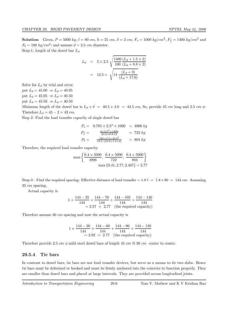
CHAPTER 29. RIGID PAVEMENT DESIGN NPTEL May 24, 2006
Solution: Given, P = 5000 kg, l = 80 cm, h = 25 cm, δ = 2 cm, Fs = 1000 kg/cm2, Ff = 1400 kg/cm2 and
Fb = 100 kg/cm2; and assume d = 2.5 cm diameter.
Step-1: length of the dowel bar Ld
Ld = 5 × 2.5
√
1400
100
(Ld + 1.5 × 2)
(Ld + 8.8 × 2)
= 12.5×
√
14(Ld + 3)
(Ld + 17.6)
Solve for Ld by trial and error:
put Ld = 45.00 ⇒ Ld = 40.95
put Ld = 45.95 ⇒ Ld = 40.50
put Ld = 45.50 ⇒ Ld = 40.50
Minimum length of the dowel bar is Ld + δ = 40.5 + 2.0 = 42.5 cm, So, provide 45 cm long and 2.5 cm φ.
Therefore Ld = 45 − 2 = 43 cm.
Step 2: Find the load transfer capacity of single dowel bar
Ps = 0.785× 2.52 × 1000 = 4906 kg
Pf = 2×2.53×1400
43.0+8.8×2= 722 kg
Pb = 100×2.5×43.02
12.5 (43.0+1.5×2)= 804 kg
Therefore, the required load transfer capacity
max
{
0.4 × 5000
4906,
0.4 × 5000
722,
0.4 × 5000
804
}
max {0.41, 2.77, 2.487} = 2.77
Step-3 : Find the required spacing: Effective distance of load transfer = 1.8 l = 1.8×80 = 144 cm. Assuming
35 cm spacing,
Actual capacity is
1 +144− 35
144+
144− 70
144+
144− 105
144+
144− 140
144= 2.57 < 2.77 (the required capacity)
Therefore assume 30 cm spacing and now the actual capacity is
1 +144− 30
144+
144− 60
144+
144− 90
144+
144− 120
144= 2.92 > 2.77 (the required capacity)
Therefore provide 2.5 cm φ mild steel dowel bars of length 45 cm @ 30 cm center to center.
29.5.4 Tie bars
In contrast to dowel bars, tie bars are not load transfer devices, but serve as a means to tie two slabs. Hence
tie bars must be deformed or hooked and must be firmly anchored into the concrete to function properly. They
are smaller than dowel bars and placed at large intervals. They are provided across longitudinal joints.
Introduction to Transportation Engineering 29.6 Tom V. Mathew and K V Krishna Rao
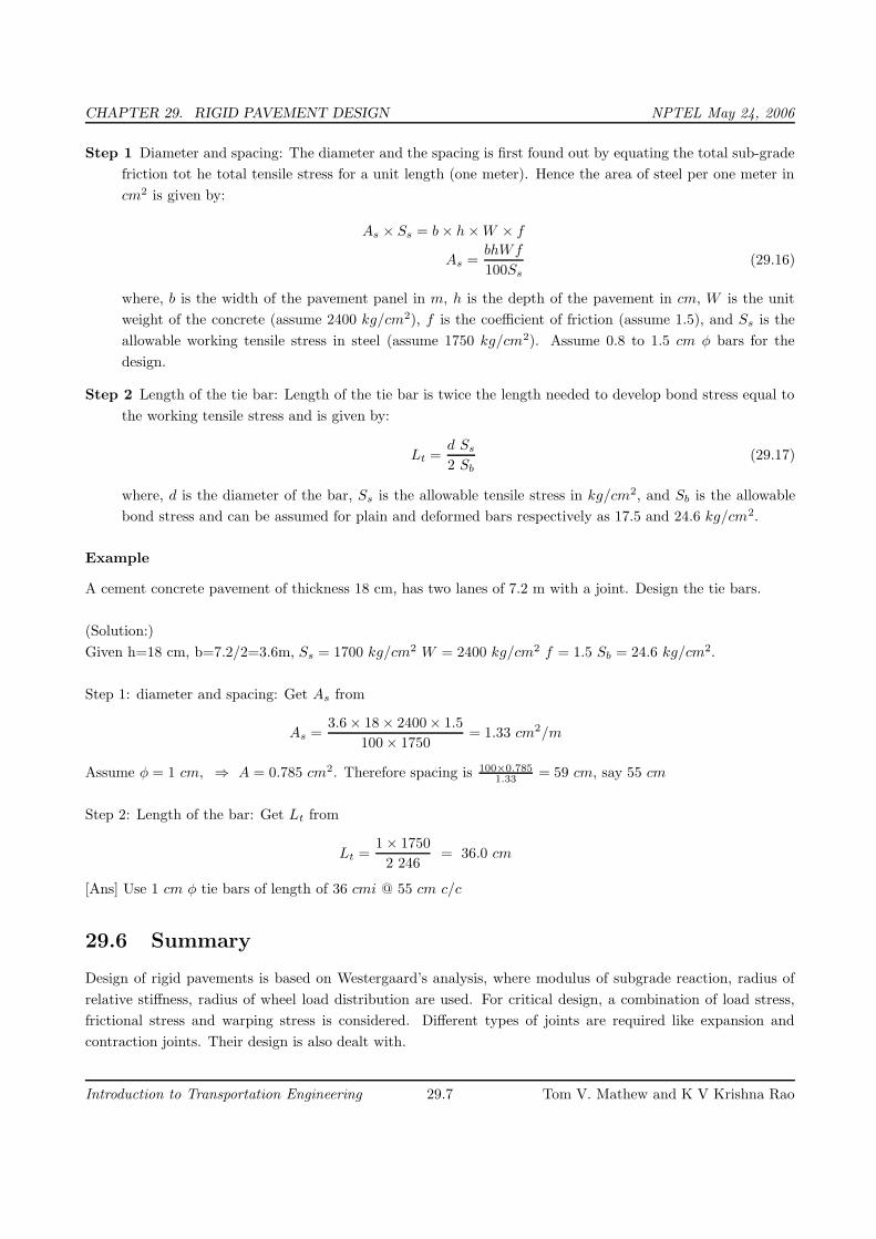
CHAPTER 29. RIGID PAVEMENT DESIGN NPTEL May 24, 2006
Step 1 Diameter and spacing: The diameter and the spacing is first found out by equating the total sub-grade
friction tot he total tensile stress for a unit length (one meter). Hence the area of steel per one meter in
cm2 is given by:
As × Ss = b × h × W × f
As =bhWf
100Ss
(29.16)
where, b is the width of the pavement panel in m, h is the depth of the pavement in cm, W is the unit
weight of the concrete (assume 2400 kg/cm2), f is the coefficient of friction (assume 1.5), and Ss is the
allowable working tensile stress in steel (assume 1750 kg/cm2). Assume 0.8 to 1.5 cm φ bars for the
design.
Step 2 Length of the tie bar: Length of the tie bar is twice the length needed to develop bond stress equal to
the working tensile stress and is given by:
Lt =d Ss
2 Sb
(29.17)
where, d is the diameter of the bar, Ss is the allowable tensile stress in kg/cm2, and Sb is the allowable
bond stress and can be assumed for plain and deformed bars respectively as 17.5 and 24.6 kg/cm2.
Example
A cement concrete pavement of thickness 18 cm, has two lanes of 7.2 m with a joint. Design the tie bars.
(Solution:)
Given h=18 cm, b=7.2/2=3.6m, Ss = 1700 kg/cm2 W = 2400 kg/cm2 f = 1.5 Sb = 24.6 kg/cm2.
Step 1: diameter and spacing: Get As from
As =3.6× 18 × 2400× 1.5
100× 1750= 1.33 cm2/m
Assume φ = 1 cm, ⇒ A = 0.785 cm2. Therefore spacing is 100×0.785
1.33= 59 cm, say 55 cm
Step 2: Length of the bar: Get Lt from
Lt =1 × 1750
2 246= 36.0 cm
[Ans] Use 1 cm φ tie bars of length of 36 cmi @ 55 cm c/c
29.6 Summary
Design of rigid pavements is based on Westergaard’s analysis, where modulus of subgrade reaction, radius of
relative stiffness, radius of wheel load distribution are used. For critical design, a combination of load stress,
frictional stress and warping stress is considered. Different types of joints are required like expansion and
contraction joints. Their design is also dealt with.
Introduction to Transportation Engineering 29.7 Tom V. Mathew and K V Krishna Rao
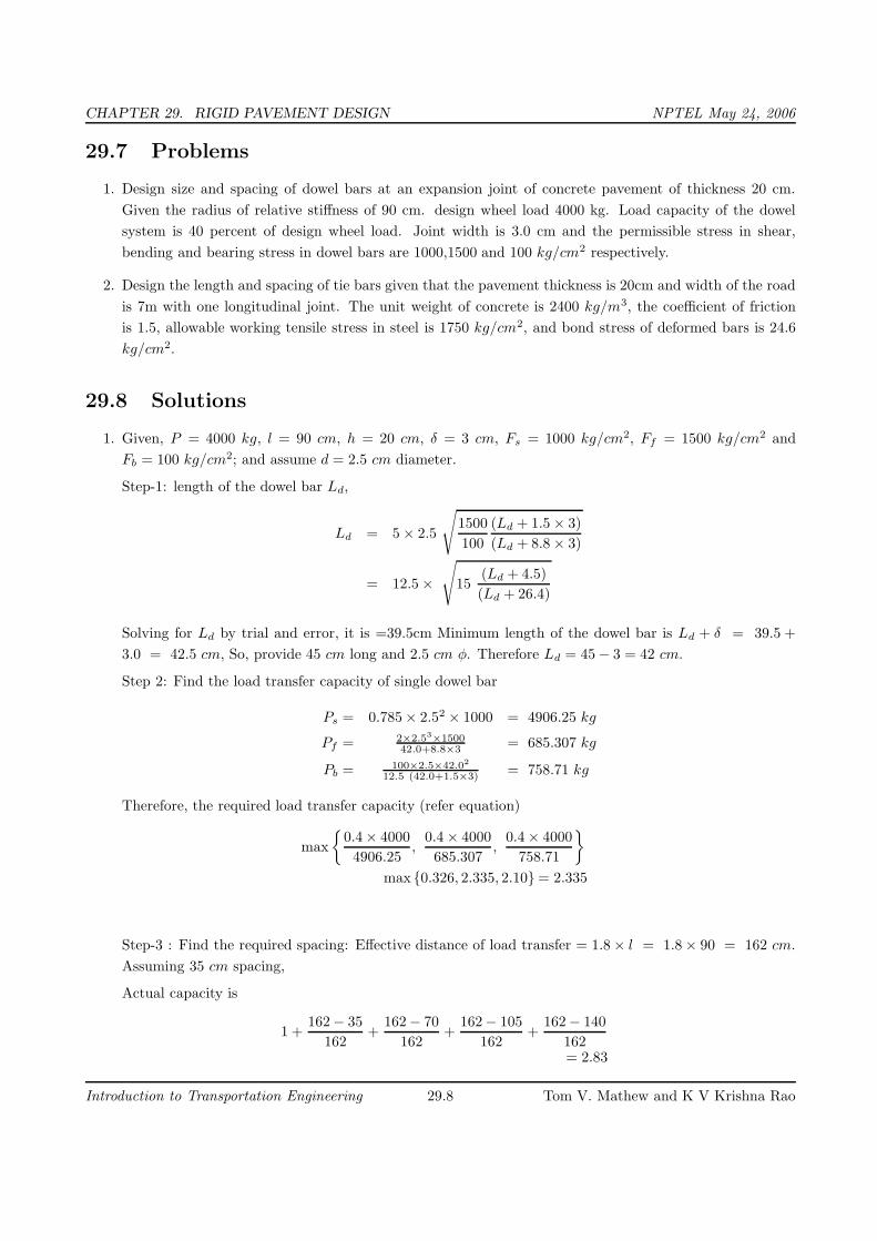
CHAPTER 29. RIGID PAVEMENT DESIGN NPTEL May 24, 2006
29.7 Problems
1. Design size and spacing of dowel bars at an expansion joint of concrete pavement of thickness 20 cm.
Given the radius of relative stiffness of 90 cm. design wheel load 4000 kg. Load capacity of the dowel
system is 40 percent of design wheel load. Joint width is 3.0 cm and the permissible stress in shear,
bending and bearing stress in dowel bars are 1000,1500 and 100 kg/cm2 respectively.
2. Design the length and spacing of tie bars given that the pavement thickness is 20cm and width of the road
is 7m with one longitudinal joint. The unit weight of concrete is 2400 kg/m3, the coefficient of friction
is 1.5, allowable working tensile stress in steel is 1750 kg/cm2, and bond stress of deformed bars is 24.6
kg/cm2.
29.8 Solutions
1. Given, P = 4000 kg, l = 90 cm, h = 20 cm, δ = 3 cm, Fs = 1000 kg/cm2, Ff = 1500 kg/cm2 and
Fb = 100 kg/cm2; and assume d = 2.5 cm diameter.
Step-1: length of the dowel bar Ld,
Ld = 5 × 2.5
√
1500
100
(Ld + 1.5 × 3)
(Ld + 8.8 × 3)
= 12.5 ×
√
15(Ld + 4.5)
(Ld + 26.4)
Solving for Ld by trial and error, it is =39.5cm Minimum length of the dowel bar is Ld + δ = 39.5 +
3.0 = 42.5 cm, So, provide 45 cm long and 2.5 cm φ. Therefore Ld = 45− 3 = 42 cm.
Step 2: Find the load transfer capacity of single dowel bar
Ps = 0.785× 2.52 × 1000 = 4906.25 kg
Pf = 2×2.53×1500
42.0+8.8×3= 685.307 kg
Pb = 100×2.5×42.02
12.5 (42.0+1.5×3)= 758.71 kg
Therefore, the required load transfer capacity (refer equation)
max
{
0.4× 4000
4906.25,
0.4 × 4000
685.307,
0.4 × 4000
758.71
}
max {0.326, 2.335, 2.10}= 2.335
Step-3 : Find the required spacing: Effective distance of load transfer = 1.8 × l = 1.8 × 90 = 162 cm.
Assuming 35 cm spacing,
Actual capacity is
1 +162− 35
162+
162− 70
162+
162− 105
162+
162− 140
162= 2.83
Introduction to Transportation Engineering 29.8 Tom V. Mathew and K V Krishna Rao
CHAPTER 29. RIGID PAVEMENT DESIGN NPTEL May 24, 2006
Assuming 40cm spacing, capacity is,
1 +162− 40
162+
162− 80
162+
162− 120
162+
162− 160
162= 2.52
So we should consider 2.52¿2.335 as it is greater and more near to other value. Therefore provide 2.5 cm φ
mild steel dowel bars of length 45 cm @ 40 cm center to center.
2. 2.Given h=20 cm, b=7/2=3.5m, Ss = 1750 kg/cm2 W = 2400 kg/cm2 f = 1.5 Sb = 24.6 kg/cm2.
Step 1: diameter and spacing:
As =3.5× 20 × 2400× 1.5
100× 1750= 1.44 cm2/m
Assume φ = 1 cm, ⇒ A = 0.785 cm2. Therefore spacing is 100×0.785
1.44= 54.57 cm, say 55 cm
Step 2: Length of the bar:
Lt =1 × 1750
2 × 24.6= 36.0 cm
[Ans] Use 1 cm φ tie bars of length of 36 cmi @ 55 cm c/c
Introduction to Transportation Engineering 29.9 Tom V. Mathew and K V Krishna Rao
CHAPTER 30. FUNDAMENTAL PARAMETERS OF TRAFFIC FLOW NPTEL May 24, 2006
Chapter 30
Fundamental parameters of traffic flow
30.1 Overview
Traffic engineering pertains to the analysis of the behavior of traffic and to design the facilities for the smooth,
safe and economical operation of traffic. Understanding traffic behavior requires a thorough knowledge of traffic
stream parameters and their mutual relationships. In this chapter the basic concepts of traffic flow is presented.
30.2 Traffic stream parameters
The traffic stream includes a combination of driver and vehicle behavior. The driver or human behavior
being non-uniform, traffic stream is also non-uniform in nature. It is influenced not only by the individual
characteristics of both vehicle and human but also by the way a group of such units interacts with each other.
Thus a flow of traffic through a street of defined characteristics will vary both by location and time corresponding
to the changes in the human behavior.
The traffic engineer, but for the purpose of planning and design, assumes that these changes are within
certain ranges which can be predicted. For example, if the maximum permissible speed of a highway is 60
kmph, the whole traffic stream can be assumed to move on an average speed of 40 kmph rather than 100 or 20
kmph.
Thus the traffic stream itself is having some parameters on which the characteristics can be predicted. The
parameters can be mainly classified as : measurements of quantity, which includes density and flow of traffic
and measurements of quality which includes speed. The traffic stream parameters can be macroscopic which
characterizes the traffic as a whole or microscopic which studies the behavior of individual vehicle in the stream
with respect to each other.
As far as the macroscopic characteristics are concerned, they can be grouped as measurement of quantity
or quality as described above, i.e. flow, density, and speed. While the microscopic characteristics include the
measures of separation, i.e. the headway or separation between vehicles which can be either time or space
headway. The fundamental stream characteristics are speed, flow, and density and are discussed below.
30.3 Speed
Speed is considered as a quality measurement of travel as the drivers and passengers will be concerned more
about the speed of the journey than the design aspects of the traffic. It is defined as the rate of motion in
Introduction to Transportation Engineering 30.1 Tom V. Mathew and K V Krishna Rao
CHAPTER 30. FUNDAMENTAL PARAMETERS OF TRAFFIC FLOW NPTEL May 24, 2006
distance per unit of time. Mathematically speed or velocity v is given by,
v =d
t(30.1)
where, v is the speed of the vehicle in m/s, d is distance traveled in m in time t seconds. Speed of different
vehicles will vary with respect to time and space. To represent these variation, several types of speed can be
defined. Important among them are spot speed, running speed, journey speed, time mean speed and space
mean speed. These are discussed below.
30.3.1 Spot Speed
Spot speed is the instantaneous speed of a vehicle at a specified location. Spot speed can be used to design
the geometry of road like horizontal and vertical curves, super elevation etc. Location and size of signs, design
of signals, safe speed, and speed zone determination, require the spot speed data. Accident analysis, road
maintenance, and congestion are the modern fields of traffic engineer, which uses spot speed data as the basic
input. Spot speed can be measured using an enoscope, pressure contact tubes or direct timing procedure or
radar speedometer or by time-lapse photographic methods. It can be determined by speeds extracted from
video images by recording the distance traveling by all vehicles between a particular pair of frames.
30.3.2 Running speed
Running speed is the average speed maintained over a particular course while the vehicle is moving and is found
by dividing the length of the course by the time duration the vehicle was in motion.
30.3.3 Journey speed
Journey speed is the effective speed of the vehicle on a journey between two points and is the distance between
the two points divided by the total time taken for the vehicle to complete the journey including any stopped
time. If the journey speed is less than running speed, it indicates that the journey follows a stop-go condition
with enforced acceleration and deceleration. The spot speed here may vary from zero to some maximum in
excess of the running speed. A uniformity between journey and running speeds denotes comfortable travel
conditions.
30.3.4 Time mean speed and space mean speed
Time mean speed is defined as the average speed of all the vehicles passing a point on a highway over some
specified time period. Space mean speed is defined as the average speed of all the vehicles occupying a given
section of a highway over some specified time period. Both mean speeds will always be different from each
other except in the unlikely event that all vehicles are traveling at the same speed. Time mean speed is a point
measurement while space mean speed is a measure relating to length of highway or lane, i.e. the mean speed
of vehicles over a period of time at a point in space is time mean speed and the mean speed over a space at a
given instant is the space mean speed.
Introduction to Transportation Engineering 30.2 Tom V. Mathew and K V Krishna Rao
CHAPTER 30. FUNDAMENTAL PARAMETERS OF TRAFFIC FLOW NPTEL May 24, 2006
30.4 Flow
There are practically two ways of counting the number of vehicles on a road. One is flow or volume, which
is defined as the number of vehicles that pass a point on a highway or a given lane or direction of a highway
during a specific time interval. The measurement is carried out by counting the number of vehicles, nt, passing
a particular point in one lane in a defined period t. Then the flow q expressed in vehicles/hour is given by
q =nt
t(30.2)
Flow is expressed in planning and design field taking a day as the measurement of time.
30.4.1 Variations of Volume
The variation of volume with time, i.e. month to month, day to day, hour to hour and within a hour is also
as important as volume calculation. Volume variations can be observed from season to season. Volume will be
above average in a pleasant motoring month of summer, but will be more pronounced in rural than in urban
area. But this is the most consistent of all the variations and affects the traffic stream characteristics the least.
Weekdays, Saturdays and Sundays will also face difference in pattern. But comparing day with day, patterns
for routes of a similar nature often show a marked similarity, which is useful in enabling predictions to be made.
The most significant variation is from hour to hour. The peak hour observed during mornings and evenings
of weekdays, which is usually 8 to 10 per cent of total daily flow or 2 to 3 times the average hourly volume.
These trips are mainly the work trips, which are relatively stable with time and more or less constant from day
to day.
30.4.2 Types of volume measurements
Since there is considerable variation in the volume of traffic, several types of measurements of volume are
commonly adopted which will average these variations into a single volume count to be used in many design
purposes.
1. Average Annual Daily Traffic(AADT) : The average 24-hour traffic volume at a given location over
a full 365-day year, i.e. the total number of vehicles passing the site in a year divided by 365.
2. Average Annual Weekday Traffic(AAWT) : The average 24-hour traffic volume occurring on week-
days over a full year. It is computed by dividing the total weekday traffic volume for the year by 260.
3. Average Daily Traffic(ADT) : An average 24-hour traffic volume at a given location for some period
of time less than a year. It may be measured for six months, a season, a month, a week, or as little as
two days. An ADT is a valid number only for the period over which it was measured.
4. Average Weekday Traffic(AWT) : An average 24-hour traffic volume occurring on weekdays for some
period of time less than one year, such as for a month or a season.
The relationship between AAWT and AWT is analogous to that between AADT and ADT. Volume in general
is measured using different ways like manual counting, detector/sensor counting, moving-car observer method,
etc. Mainly the volume study establishes the importance of a particular route with respect to the other routes,
the distribution of traffic on road, and the fluctuations in flow. All which eventually determines the design of
a highway and the related facilities. Thus, volume is treated as the most important of all the parameters of
traffic stream.
Introduction to Transportation Engineering 30.3 Tom V. Mathew and K V Krishna Rao
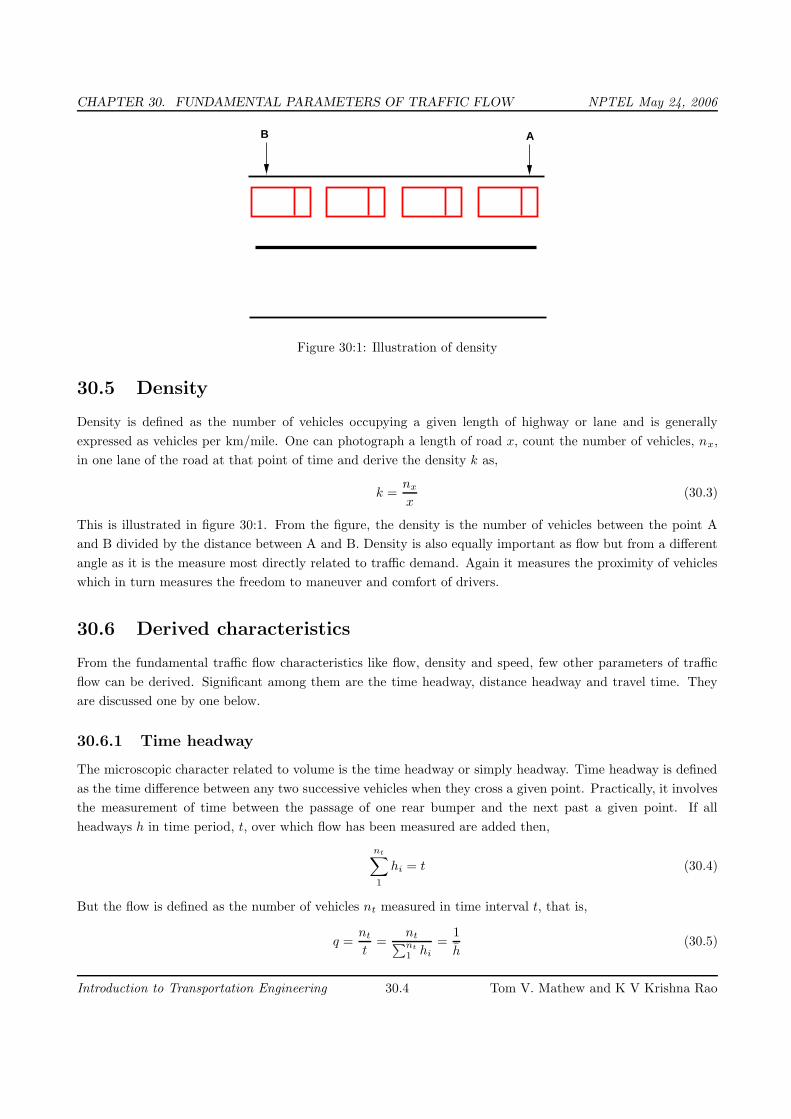
CHAPTER 30. FUNDAMENTAL PARAMETERS OF TRAFFIC FLOW NPTEL May 24, 2006
B A
Figure 30:1: Illustration of density
30.5 Density
Density is defined as the number of vehicles occupying a given length of highway or lane and is generally
expressed as vehicles per km/mile. One can photograph a length of road x, count the number of vehicles, nx,
in one lane of the road at that point of time and derive the density k as,
k =nx
x(30.3)
This is illustrated in figure 30:1. From the figure, the density is the number of vehicles between the point A
and B divided by the distance between A and B. Density is also equally important as flow but from a different
angle as it is the measure most directly related to traffic demand. Again it measures the proximity of vehicles
which in turn measures the freedom to maneuver and comfort of drivers.
30.6 Derived characteristics
From the fundamental traffic flow characteristics like flow, density and speed, few other parameters of traffic
flow can be derived. Significant among them are the time headway, distance headway and travel time. They
are discussed one by one below.
30.6.1 Time headway
The microscopic character related to volume is the time headway or simply headway. Time headway is defined
as the time difference between any two successive vehicles when they cross a given point. Practically, it involves
the measurement of time between the passage of one rear bumper and the next past a given point. If all
headways h in time period, t, over which flow has been measured are added then,
nt∑
1
hi = t (30.4)
But the flow is defined as the number of vehicles nt measured in time interval t, that is,
q =nt
t=
nt∑
nt
1hi
=1
h(30.5)
Introduction to Transportation Engineering 30.4 Tom V. Mathew and K V Krishna Rao
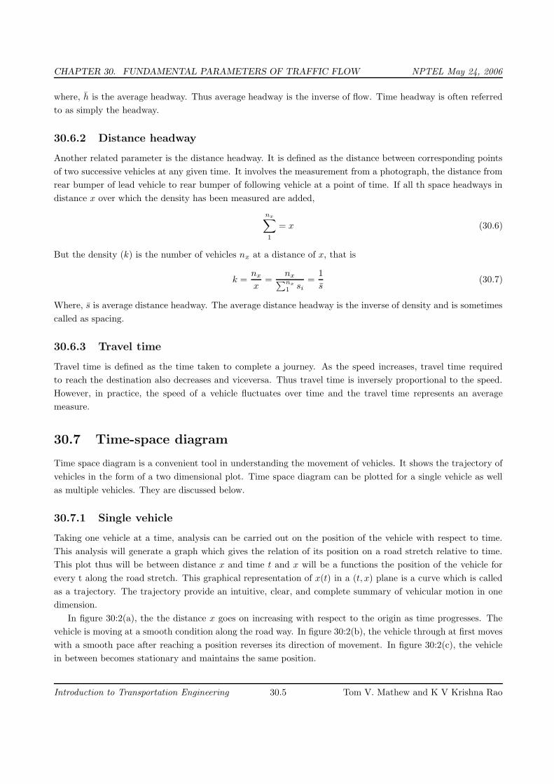
CHAPTER 30. FUNDAMENTAL PARAMETERS OF TRAFFIC FLOW NPTEL May 24, 2006
where, h is the average headway. Thus average headway is the inverse of flow. Time headway is often referred
to as simply the headway.
30.6.2 Distance headway
Another related parameter is the distance headway. It is defined as the distance between corresponding points
of two successive vehicles at any given time. It involves the measurement from a photograph, the distance from
rear bumper of lead vehicle to rear bumper of following vehicle at a point of time. If all th space headways in
distance x over which the density has been measured are added,
nx∑
1
= x (30.6)
But the density (k) is the number of vehicles nx at a distance of x, that is
k =nx
x=
nx∑
nx
1si
=1
s(30.7)
Where, s is average distance headway. The average distance headway is the inverse of density and is sometimes
called as spacing.
30.6.3 Travel time
Travel time is defined as the time taken to complete a journey. As the speed increases, travel time required
to reach the destination also decreases and viceversa. Thus travel time is inversely proportional to the speed.
However, in practice, the speed of a vehicle fluctuates over time and the travel time represents an average
measure.
30.7 Time-space diagram
Time space diagram is a convenient tool in understanding the movement of vehicles. It shows the trajectory of
vehicles in the form of a two dimensional plot. Time space diagram can be plotted for a single vehicle as well
as multiple vehicles. They are discussed below.
30.7.1 Single vehicle
Taking one vehicle at a time, analysis can be carried out on the position of the vehicle with respect to time.
This analysis will generate a graph which gives the relation of its position on a road stretch relative to time.
This plot thus will be between distance x and time t and x will be a functions the position of the vehicle for
every t along the road stretch. This graphical representation of x(t) in a (t, x) plane is a curve which is called
as a trajectory. The trajectory provide an intuitive, clear, and complete summary of vehicular motion in one
dimension.
In figure 30:2(a), the the distance x goes on increasing with respect to the origin as time progresses. The
vehicle is moving at a smooth condition along the road way. In figure 30:2(b), the vehicle through at first moves
with a smooth pace after reaching a position reverses its direction of movement. In figure 30:2(c), the vehicle
in between becomes stationary and maintains the same position.
Introduction to Transportation Engineering 30.5 Tom V. Mathew and K V Krishna Rao
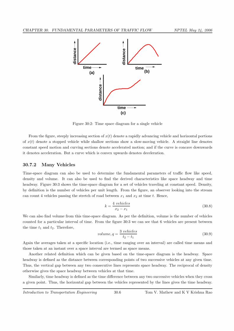
CHAPTER 30. FUNDAMENTAL PARAMETERS OF TRAFFIC FLOW NPTEL May 24, 2006
(a) (b)
(c)
time
dis
tan
ce
dis
tan
ce
time
dis
tan
ce
time
Figure 30:2: Time space diagram for a single vehicle
From the figure, steeply increasing section of x(t) denote a rapidly advancing vehicle and horizontal portions
of x(t) denote a stopped vehicle while shallow sections show a slow-moving vehicle. A straight line denotes
constant speed motion and curving sections denote accelerated motion; and if the curve is concave downwards
it denotes acceleration. But a curve which is convex upwards denotes deceleration.
30.7.2 Many Vehicles
Time-space diagram can also be used to determine the fundamental parameters of traffic flow like speed,
density and volume. It can also be used to find the derived characteristics like space headway and time
headway. Figure 30:3 shows the time-space diagram for a set of vehicles traveling at constant speed. Density,
by definition is the number of vehicles per unit length. From the figure, an observer looking into the stream
can count 4 vehicles passing the stretch of road between x1 and x2 at time t. Hence,
k =4 vehicles
x2 − x1
(30.8)
We can also find volume from this time-space diagram. As per the definition, volume is the number of vehicles
counted for a particular interval of time. From the figure 30:3 we can see that 6 vehicles are present between
the time t1 and t2. Therefore,
volume, q =3 vehicles
t2 − t1(30.9)
Again the averages taken at a specific location (i.e., time ranging over an interval) are called time means and
those taken at an instant over a space interval are termed as space means.
Another related definition which can be given based on the time-space diagram is the headway. Space
headway is defined as the distance between corresponding points of two successive vehicles at any given time.
Thus, the vertical gap between any two consecutive lines represents space headway. The reciprocal of density
otherwise gives the space headway between vehicles at that time.
Similarly, time headway is defined as the time difference between any two successive vehicles when they cross
a given point. Thus, the horizontal gap between the vehicles represented by the lines gives the time headway.
Introduction to Transportation Engineering 30.6 Tom V. Mathew and K V Krishna Rao
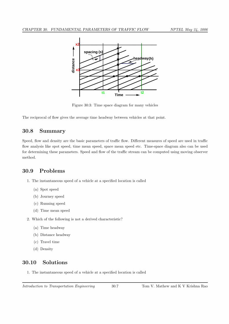
CHAPTER 30. FUNDAMENTAL PARAMETERS OF TRAFFIC FLOW NPTEL May 24, 2006
tTime
(h)headway
x1
x2
dis
tan
ce
t1 t2
(s)spacing
Figure 30:3: Time space diagram for many vehicles
The reciprocal of flow gives the average time headway between vehicles at that point.
30.8 Summary
Speed, flow and density are the basic parameters of traffic flow. Different measures of speed are used in traffic
flow analysis like spot speed, time mean speed, space mean speed etc. Time-space diagram also can be used
for determining these parameters. Speed and flow of the traffic stream can be computed using moving observer
method.
30.9 Problems
1. The instantaneous speed of a vehicle at a specified location is called
(a) Spot speed
(b) Journey speed
(c) Running speed
(d) Time mean speed
2. Which of the following is not a derived characteristic?
(a) Time headway
(b) Distance headway
(c) Travel time
(d) Density
30.10 Solutions
1. The instantaneous speed of a vehicle at a specified location is called
Introduction to Transportation Engineering 30.7 Tom V. Mathew and K V Krishna Rao
CHAPTER 30. FUNDAMENTAL PARAMETERS OF TRAFFIC FLOW NPTEL May 24, 2006
(a) Spot speed√
(b) Journey speed
(c) Running speed
(d) Time mean speed
2. Which of the following is not a derived characteristic?
(a) Time headway
(b) Distance headway
(c) Travel time
(d) Density√
Introduction to Transportation Engineering 30.8 Tom V. Mathew and K V Krishna Rao
CHAPTER 31. FUNDAMENTAL RELATIONS OF TRAFFIC FLOW NPTEL May 24, 2006
Chapter 31
Fundamental relations of traffic flow
31.1 Overview
Speed is one of the basic parameters of traffic flow and time mean speed and space mean speed are the two
representations of speed. Time mean speed and space mean speed and the relationship between them will be
discussed in detail in this chapter. The relationship between the fundamental parameters of traffic flow will
also be derived. In addition, this relationship can be represented in graphical form resulting in the fundamental
diagrams of traffic flow.
31.2 Time mean speed (vt)
As noted earlier, time mean speed is the average of all vehicles passing a point over a duration of time. It is
the simple average of spot speed. Time mean speed vt is given by,
vt =1
n
n∑
i=1
vi, (31.1)
where v is the spot speed of ith vehicle, and n is the number of observations. In many speed studies, speeds are
represented in the form of frequency table. Then the time mean speed is given by,
vt =
∑
n
i=1qivi
∑
n
i=1qi
, (31.2)
where qi is the number of vehicles having speed vi, and n is the number of such speed categories.
31.3 Space mean speed (vs)
The space mean speed also averages the spot speed, but spatial weightage is given instead of temporal. This is
derived as below. Consider unit length of a road, and let vi is the spot speed of ith vehicle. Let ti is the time
the vehicle takes to complete unit distance and is given by 1
vi
. If there are n such vehicles, then the average
travel time ts is given by,
ts =Σti
n=
1
nΣ
1
vi
(31.3)
If tav is the average travel time, then average speed vs = 1
ts
. Therefore from the above equation,
vs =n
∑
n
i=1
1
vi
(31.4)
Introduction to Transportation Engineering 31.1 Tom V. Mathew and K V Krishna Rao
CHAPTER 31. FUNDAMENTAL RELATIONS OF TRAFFIC FLOW NPTEL May 24, 2006
No. speed range average speed (vi) volume of flow (qi) viqiqi
vi
1 2-5 3.5 1 3.5 2.29
2 6-9 7.5 4 30.0 0.54
3 10-13 11.5 0 0 0
4 14-17 15.5 7 108.5 0.45
total 12 142 3.28
This is simply the harmonic mean of the spot speed. If the spot speeds are expressed as a frequency table, then,
vs =
∑
n
i=1qi
∑
n
i=1
qi
vi
(31.5)
where qi vehicle will have vi speed and ni is the number of such observations.
Example 1
If the spot speeds are 50, 40, 60,54 and 45, then find the time mean speed and space mean speed.
Solution Time mean speed vt is the average of spot speed. Therefore, vt = Σvi
n= 50+40+60+54+45
5= 249
5= 49.8
Space mean speed is the harmonic mean of spot speed.Therefore, vs = n
Σ1
vi
= 51
50+
1
40+
1
60+
1
54+
1
45
= 5
0.12= 48.82
Example 2
The results of a speed study is given in the form of a frequency distribution table. Find the time mean speed
and space mean speed.
speed range frequency
2-5 1
6-9 4
10-13 0
14-17 7
Solution The time mean speed and space mean speed can be found out from the frequency table given
below. First, the average speed is computed, which is the mean of the speed range. For example, for the
first speed range, average speed, vi = 2+5
2= 3.5 seconds. The volume of flow qi for that speed range is same
as the frequency. The terms vi.qi and qi
vi
are also tabulated, and their summations in the last row. Time
mean speed can be computed as, vt = Σqivi
Σqi
= 142
12= 11.83 Similarly, space mean speed can be computed as,
vs = Σqi
Σqi
vi
= 12
3.28= 3.65
31.4 Illustration of mean speeds
Inorder to understand the concept of time mean speed and space mean speed, following illustration will help.
Let there be a road stretch having two sets of vehicle as in figure 31:1. The first vehicle is traveling at 10m/s
with 50 m spacing, and the second set at 20m/s with 100 m spacing. Therefore, the headway of the slow vehicle
Introduction to Transportation Engineering 31.2 Tom V. Mathew and K V Krishna Rao
CHAPTER 31. FUNDAMENTAL RELATIONS OF TRAFFIC FLOW NPTEL May 24, 2006
10 m/s 10 m/s 10 m/s 10 m/s 10 m/s
20 m/s20 m/s20 m/s
100 100
5050 5050
Figure 31:1: Illustration of relation between time mean speed and space mean speed
hs will be 50 m divided by 10 m/s which is 5 sec. Therefore, the number of slow moving vehicles observed at A
in one hour ns will be 60/5 = 12 vehicles. The density K is the number of vehicles in 1 km, and is the inverse
of spacing. Therefore, Ks = 1000/50 = 20 vehicles/km. Therefore, by definition, time mean speed vt is given
by vt = 12×10+12×5
24= 15 m/s. Similarly, by definition, space mean speed is the mean of vehicle speeds over
time. Therefore, vs = 20×10+10×20
30= 13.3 m/s This is same as the harmonic mean of spot speeds obtained
at location A; ie vs = 24
12×1
10+12×
1
20
= 13.3 m/s. It may be noted that since harmonic mean is always lower
than the arithmetic mean, and also as observed , space mean speed is always lower than the time mean speed.
In other words, space mean speed weights slower vehicles more heavily as they occupy they occupy the road
stretch for longer duration of time. For this reason, in many fundamental traffic equations, space mean speed
is preferred over time mean speed.
31.5 Relation between time mean speed and space mean speed
The relation between time mean speed and space mean speed can be derived as below. Consider a stream of
vehicles with a set of substream flow q1,q2, . . . qi, . . . qn having speed v1,v2, . . . vi, . . . vn. The fundamental
relation between flow(q), density(k) and mean speed vs is,
q = k × vs (31.6)
Therefore for any substream qi, the following relationship will be valid.
qi = ki × vi (31.7)
The summation of all substream flows will give the total flow q.
Σqi = q (31.8)
Similarly the summation of all substream density will give the total density k.
Σki = k (31.9)
Let fi denote the proportion of substream density ki to the total density k,
fi =ki
k(31.10)
Space mean speed averages the speed over space. Therefore, if ki vehicles has vi speed, then space mean speed
is given by,
vs =Σkivi
k(31.11)
Introduction to Transportation Engineering 31.3 Tom V. Mathew and K V Krishna Rao
CHAPTER 31. FUNDAMENTAL RELATIONS OF TRAFFIC FLOW NPTEL May 24, 2006
Time mean speed averages the speed over time.Therefore,
vt =Σqivi
q(31.12)
Substituting in 31.7 vt can be written as,
vt =Σkivi
2
q(31.13)
Rewriting the above equation and substituting 31.11, and then substituting 31.6, we get,
vt = kΣki
kv2
i
=kΣfivi
2
q
=Σfivi
2
vs
By adding and subtracting vs and doing algebraic manipulations, vt can be written as,
vt =Σfi(vs + (vi − vs))
2
vs
(31.14)
=Σfi(vs)
2 + (vi − vs)2 + 2.vs.(vi − vs)
vs
(31.15)
=Σfivs
2
vs
+Σfi(vi − vs)
2
vs
+2.vs.Σfi(vi − vs)
vs
(31.16)
The third term of the equation will be zero because Σfi(vi − vs) will be zero, since vs is the mean speed of vi.
The numerator of the second term gives the standard deviation of vi. Σfi by definition is 1.Therefore,
= vsΣfi +σ2
vs
+ 0 (31.17)
vt = vs +σ2
vs
(31.18)
Hence, time mean speed is space mean speed plus standard deviation of the spot speed divided by the space
mean speed. Time mean speed will be always greater than space mean speed since standard deviation cannot
be negative. If all the speed of the vehicles are the same, then spot speed, time mean speed and space mean
speed will also be same.
31.6 Fundamental relations of traffic flow
The relationship between the fundamental variables of traffic flow, namely speed, volume, and density is called
the fundamental relations of traffic flow. This can be derived by a simple concept. Let there be a road with
length v km, and assume all the vehicles are moving with v km/hr.(Fig 31:2). Let the number of vehicles
counted by an observer at A for one hour be n1. By definition, the number of vehicles counted in one hour is
flow(q). Therefore,
n1 = q (31.19)
Introduction to Transportation Engineering 31.4 Tom V. Mathew and K V Krishna Rao
CHAPTER 31. FUNDAMENTAL RELATIONS OF TRAFFIC FLOW NPTEL May 24, 2006
8
Bv km
67 5 4 3 2 1
Figure 31:2: Illustration of relation between time mean speed and space mean speed
Similarly, by definition, density is the number of vehicles in unit distance. Therefore number of vehicles n2
in a road stretch of distance v1 will be density × distance.Therefore,
n2 = k × v (31.20)
Since all the vehicles have speed v, the number of vehicles counted in 1 hour and the number of vehicles in the
stretch of distance v will also be same.(ie n1 = n2). Therefore,
q = k × v (31.21)
This is the fundamental equation of traffic flow. Please note that, v in the above equation refers to the space
mean speed.
31.7 Fundamental diagrams of traffic flow
The relation between flow and density, density and speed, speed and flow, can be represented with the help of
some curves. They are referred to as the fundamental diagrams of traffic flow. They will be explained in detail
one by one below.
31.7.1 Flow-density curve
The flow and density varies with time and location. The relation between the density and the corresponding flow
on a given stretch of road is referred to as one of the fundamental diagram of traffic flow. Some characteristics
of an ideal flow-density relationship is listed below:
1. When the density is zero, flow will also be zero,since there is no vehicles on the road.
2. When the number of vehicles gradually increases the density as well as flow increases.
3. When more and more vehicles are added, it reaches a situation where vehicles can’t move. This is referred
to as the jam density or the maximum density. At jam density, flow will be zero because the vehicles are
not moving.
4. There will be some density between zero density and jam density, when the flow is maximum. The
relationship is normally represented by a parabolic curve as shown in figure 31:3
The point O refers to the case with zero density and zero flow. The point B refers to the maximum flow and the
corresponding density is kmax. The point C refers to the maximum density kjam and the corresponding flow
is zero. OA is the tangent drawn to the parabola at O, and the slope of the line OA gives the mean free flow
Introduction to Transportation Engineering 31.5 Tom V. Mathew and K V Krishna Rao
CHAPTER 31. FUNDAMENTAL RELATIONS OF TRAFFIC FLOW NPTEL May 24, 2006
B
A
CO
EDq
density (k)
flo
w(q
)
k0 k1 kmax k2
qmax
kjam
Figure 31:3: Flow density curve
spee
d u
density (k)k0kjam
uf
Figure 31:4: Speed-density diagram
speed, ie the speed with which a vehicle can travel when there is no flow. It can also be noted that points D
and E correspond to same flow but has two different densities. Further, the slope of the line OD gives the mean
speed at density k1 and slope of the line OE will give mean speed at density k2. Clearly the speed at density
k1 will be higher since there are less number of vehicles on the road.
31.7.2 Speed-density diagram
Similar to the flow-density relationship, speed will be maximum, referred to as the free flow speed, and when
the density is maximum, the speed will be zero. The most simple assumption is that this variation of speed
with density is linear as shown by the solid line in figure 31:4. Corresponding to the zero density, vehicles will
be flowing with their desire speed, or free flow speed. When the density is jam density, the speed of the vehicles
becomes zero. It is also possible to have non-linear relationships as shown by the dotted lines. These will be
discussed later.
Introduction to Transportation Engineering 31.6 Tom V. Mathew and K V Krishna Rao
CHAPTER 31. FUNDAMENTAL RELATIONS OF TRAFFIC FLOW NPTEL May 24, 2006
flow q
q
usp
eed
u
Qmaxu0
u1
u2
uf
Figure 31:5: Speed-flow diagram
spee
d u
flow q
flo
w q
density k
spee
d u
density k qmax
Figure 31:6: Fundamental diagram of traffic flow
31.7.3 Speed flow relation
The relationship between the speed and flow can be postulated as follows. The flow is zero either because there
is no vehicles or there are too many vehicles so that they cannot move. At maximum flow, the speed will be in
between zero and free flow speed. This relationship is shown in figure 31:5. The maximum flow qmax occurs at
speed u. It is possible to have two different speeds for a given flow.
31.7.4 Combined diagrams
The diagrams shown in the relationship between speed-flow, speed-density, and flow-density are called the
fundamental diagrams of traffic flow. These are as shown in figure 31:6
Introduction to Transportation Engineering 31.7 Tom V. Mathew and K V Krishna Rao
CHAPTER 31. FUNDAMENTAL RELATIONS OF TRAFFIC FLOW NPTEL May 24, 2006
31.8 Summary
Time mean speed and space mean speed are two important measures of speed. It is possible to have a relation
between them and was derived in this chapter. Also, time mean speed will be always greater than or equal to
space mean speed. The fundamental diagrams of traffic flow are vital tools which enables analysis of fundamental
relationships. There are three diagrams - speed-density, speed-flow and flow-density. They can be together
combined in a single diagram as discussed in the last section of the chapter.
31.9 Problems
1. Space mean speed is
(a) the harmonic mean of spot speeds
(b) the sum of spot speeds
(c) the arithmetic mean of spot speeds
(d) the sum of journey speeds
2. Which among the following is the fundamental equation of traffic flow?
(a) q = k
v
(b) q = k × v
(c) v = q × k
(d) q = k2 × v
31.10 Solutions
1. Space mean speed is
(a) the harmonic mean of spot speeds√
(b) the sum of spot speeds
(c) the arithmetic mean of spot speeds
(d) the sum of journey speeds
2. Which among the following is the fundamental equation of traffic flow?
(a) q = k
v
(b) q = k × v√
(c) v = q × k
(d) q = k2 × v
Introduction to Transportation Engineering 31.8 Tom V. Mathew and K V Krishna Rao
CHAPTER 32. TRAFFIC DATA COLLECTION NPTEL May 24, 2006
Chapter 32
Traffic data collection
32.1 Overview
Unlike many other disciplines of the engineering, the situations that are interesting to a traffic engineer cannot
be reproduced in a laboratory. Even if road and vehicles could be set up in large laboratories, it is impossible to
simulate the behavior of drivers in the laboratory. Therefore, traffic stream characteristics need to be collected
only from the field. There are several methods of data collection depending on the need of the study and some
important ones are described in this chapter.
32.2 Data requirements
The most important traffic characteristics to be collected from the field includes sped, travel time, flow and
density. Some cases, spacing and headway are directly measured. In addition, the occupancy, ie percentage
of time a point on the road is occupied by vehicles is also of interest. The measurement procedures can be
classified based on the geographical extent of the survey into five categories: (a) measurement at point on the
road, (b) measurement over a short section of the road (less than 500 metres) (c) measurement over a length of
the road (more than about 500 metres) (d) wide area samples obtained from number of locations, and (e) the
use of an observer moving in the traffic stream. In each category, numerous data collection are there. However,
important and basic methods will be discussed.
32.2.1 Measurements at a point
The most important point measurement is the vehicle volume count. Data can be collected manually or
automatically. In manual method, the observer will stand at the point of interest and count the vehicles with
the help of hand tallies. Normally, data will be collected for short interval of 5 minutes or 15 minutes etc. and
for each types of vehicles like cars, two wheelers, three wheelers, LCV, HCV, multi axle trucks, nonmotorised
traffic like bullock cart, hand cart etc. From the flow data, flow and headway can be derived.
Modern methods include the use of inductive loop detector, video camera, and many other technologies.
These methods helps to collect accurate information for long duration. In video cameras, data is collected from
the field and is then analyzed in the lab for obtaining results. Radars and microwave detectors are used to
obtain the speed of a vehicle at a point. Since no length is involved, density cannot be obtained by measuring
at a point.
Introduction to Transportation Engineering 32.1 Tom V. Mathew and K V Krishna Rao
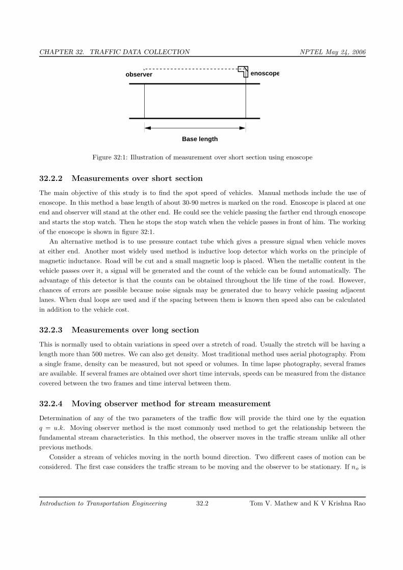
CHAPTER 32. TRAFFIC DATA COLLECTION NPTEL May 24, 2006
x
Base length
observer enoscope
Figure 32:1: Illustration of measurement over short section using enoscope
32.2.2 Measurements over short section
The main objective of this study is to find the spot speed of vehicles. Manual methods include the use of
enoscope. In this method a base length of about 30-90 metres is marked on the road. Enoscope is placed at one
end and observer will stand at the other end. He could see the vehicle passing the farther end through enoscope
and starts the stop watch. Then he stops the stop watch when the vehicle passes in front of him. The working
of the enoscope is shown in figure 32:1.
An alternative method is to use pressure contact tube which gives a pressure signal when vehicle moves
at either end. Another most widely used method is inductive loop detector which works on the principle of
magnetic inductance. Road will be cut and a small magnetic loop is placed. When the metallic content in the
vehicle passes over it, a signal will be generated and the count of the vehicle can be found automatically. The
advantage of this detector is that the counts can be obtained throughout the life time of the road. However,
chances of errors are possible because noise signals may be generated due to heavy vehicle passing adjacent
lanes. When dual loops are used and if the spacing between them is known then speed also can be calculated
in addition to the vehicle cost.
32.2.3 Measurements over long section
This is normally used to obtain variations in speed over a stretch of road. Usually the stretch will be having a
length more than 500 metres. We can also get density. Most traditional method uses aerial photography. From
a single frame, density can be measured, but not speed or volumes. In time lapse photography, several frames
are available. If several frames are obtained over short time intervals, speeds can be measured from the distance
covered between the two frames and time interval between them.
32.2.4 Moving observer method for stream measurement
Determination of any of the two parameters of the traffic flow will provide the third one by the equation
q = u.k. Moving observer method is the most commonly used method to get the relationship between the
fundamental stream characteristics. In this method, the observer moves in the traffic stream unlike all other
previous methods.
Consider a stream of vehicles moving in the north bound direction. Two different cases of motion can be
considered. The first case considers the traffic stream to be moving and the observer to be stationary. If no is
Introduction to Transportation Engineering 32.2 Tom V. Mathew and K V Krishna Rao
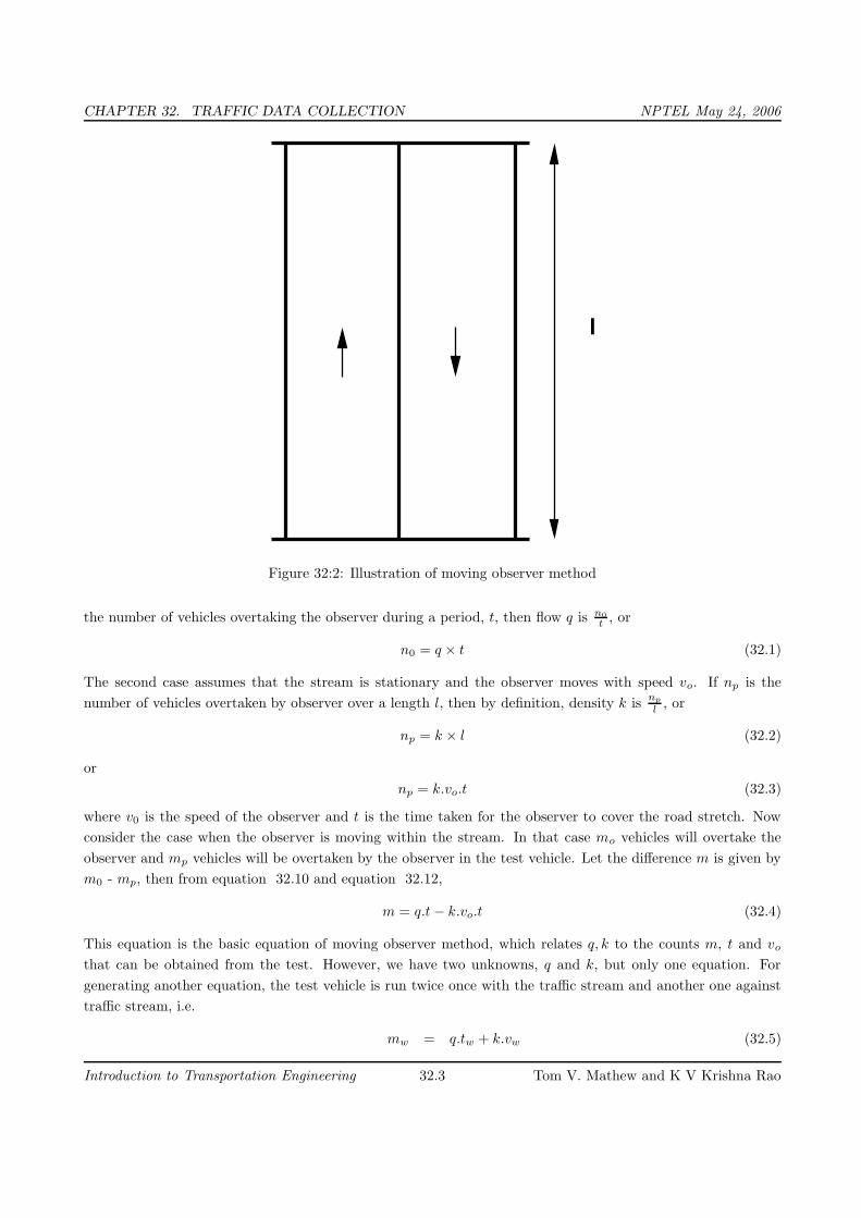
CHAPTER 32. TRAFFIC DATA COLLECTION NPTEL May 24, 2006
l
Figure 32:2: Illustration of moving observer method
the number of vehicles overtaking the observer during a period, t, then flow q is n0
t, or
n0 = q × t (32.1)
The second case assumes that the stream is stationary and the observer moves with speed vo. If np is the
number of vehicles overtaken by observer over a length l, then by definition, density k isnp
l, or
np = k × l (32.2)
or
np = k.vo.t (32.3)
where v0 is the speed of the observer and t is the time taken for the observer to cover the road stretch. Now
consider the case when the observer is moving within the stream. In that case mo vehicles will overtake the
observer and mp vehicles will be overtaken by the observer in the test vehicle. Let the difference m is given by
m0 - mp, then from equation 32.10 and equation 32.12,
m = q.t − k.vo.t (32.4)
This equation is the basic equation of moving observer method, which relates q, k to the counts m, t and vo
that can be obtained from the test. However, we have two unknowns, q and k, but only one equation. For
generating another equation, the test vehicle is run twice once with the traffic stream and another one against
traffic stream, i.e.
mw = q.tw + k.vw (32.5)
Introduction to Transportation Engineering 32.3 Tom V. Mathew and K V Krishna Rao
CHAPTER 32. TRAFFIC DATA COLLECTION NPTEL May 24, 2006
nonumber = q.tw + k.l (32.6)
ma = qta − k.va (32.7)
nonumber = q.ta − k.l (32.8)
(32.9)
where, a, w denotes against and with traffic flow. It may be noted that the sign of equation 32.8 is negative,
because test vehicle moving in the opposite direction can be considered as a case when the test vehicle is moving
in the stream with negative velocity. Further, in this case, all the vehicles will be overtaking, since it is moving
with negative speed. In other words, when the test vehicle moves in the opposite direction, the observer simply
counts the number of vehicles in the opposite direction. Adding equation 32.6 and 32.8, we will get the first
parameter of the stream, namely the flow(q) as:
q =mw + ma
tw + ta(32.10)
Now calculating space mean speed from equation 32.6,
mw
tw= q − k.vw
= q −q
vvw
= q −q
v
[
l
tw
]
= q(1 −l
v×
1
tw)
= q(1 −tavg
tw)
If vs is the mean stream speed, then average travel time is given by tavg = l
vs
. Therefore,
mw
q= tw(1 −
tavg
tw) = tw − tavg
tavg = tw −mw
q=
l
v,
Rewriting the above equation, we get the second parameter of the traffic flow, namely the mean speed vs and
can be written as,
vs =l
tw − mw
q
(32.11)
Thus two parameters of the stream can be determined. Knowing the two parameters the third parameter of
traffic flow density (k) can be found out as
k =q
vs
(32.12)
For increase accuracy and reliability, the test is performed a number of times and the average results are to be
taken.
Example 1
The length of a road stretch used for conducting the moving observer test is 0.5 km and the speed with which
the test vehicle moved is 20 km/hr. Given that the number of vehicles encountered in the stream while the test
Introduction to Transportation Engineering 32.4 Tom V. Mathew and K V Krishna Rao
CHAPTER 32. TRAFFIC DATA COLLECTION NPTEL May 24, 2006
Sample no. ma mo mp m(mo − mp) ta tw q = ma+mw
ta+tw
u = l
tw−
ma
q
k = q
v
1 107 10 74 -64 0.025 0.025 860 5.03 171
2 113 25 41 -16 0.025 0.025 1940 15.04 129
3 30 15 5 10 0.025 0.025 800 40 20
4 79 18 9 9 0.025 0.025 1760 25.14 70
vehicle was moving against the traffic stream is 107, number of vehicles that had overtaken the test vehicle is
10, and the number of vehicles overtaken by the test vehicle is 74, find the flow, density and average speed of
the stream.
Solution Time taken by the test vehicle to reach the other end of the stream while it is moving along with
the traffic is tw = 0.5
20= 0.025 hr Time taken by the observer to reach the other end of the stream while it is
moving against the traffic is ta = tw = 0.025 hr Flow is given by equation, q = 107+(10−74)
0.025+0.025= 860 veh/hr Stream
speed vs can be found out from equationvs = 0.5
0.025−10.74
860
= 5 km/hr Density can be found out from equation as
k = 860
5= 172veh/km
Example 2
The data from four moving observer test methods are shown in the table. Column 1 gives the sample number,
column 2 gives the number of vehicles moving against the stream, column 3 gives the number of vehicles that
had overtaken the test vehicle, and last column gives the number of vehicles overtaken by the test vehicle. Find
the three fundamental stream parameters for each set of data. Also plot the fundamental diagrams of traffic
flow.
Sample no. 1 2 3
1 107 10 74
2 113 25 41
3 30 15 5
4 79 18 9
Solution From the calculated values of flow, density and speed, the three fundamental diagrams can be
plotted as shown in figure 32:3.
32.3 Summary
Traffic engineering studies differ from other studies in the fact that they require extensive data from the field
which cannot be exactly created in any laboratory. Speed data are collected from measurements at a point or
over a short section or over an area. Traffic flow data are collected at a point. Moving observer method is one
in which both speed and traffic flow data are obtained by a single experiment.
Introduction to Transportation Engineering 32.5 Tom V. Mathew and K V Krishna Rao
CHAPTER 32. TRAFFIC DATA COLLECTION NPTEL May 24, 2006
density k
flo
w q
20 70129171
800
1760
1940
flow q
spee
d u
860
40
density k5.03
15.0425.14
spee
d u
Figure 32:3: Fundamental diagrams of traffic flow
32.4 Problems
1. In the moving observer experiment, if the density is k, speed of the observer is vo , length of the test
stretch is l, t is the time taken by the observer to cover the road stretch, the number of vehicles overtaken
by the observer np is given by,
(a) np = k.t
(b) np = k.l
(c) np = k
vo.t
(d) np = k.vo.t
2. If the length of the road stretch taken for conducting moving observer experiment is 0.4 km, time taken
by the observer to move with the traffic is 5 seconds, number of vehicles moving with the test vehicle in
the same direction is 10, flow is 10 veh/sec, find the mean speed.
(a) 50 m/s
(b) 100 m/s
(c) 150 m/s
(d) 200 m/s
32.5 Solutions
1. In the moving observer experiment, if the density is k, speed of the observer is vo , length of the test
stretch is l, t is the time taken by the observer to cover the road stretch, the number of vehicles overtaken
by the observer np is given by,
(a) np = k.t
Introduction to Transportation Engineering 32.6 Tom V. Mathew and K V Krishna Rao
CHAPTER 32. TRAFFIC DATA COLLECTION NPTEL May 24, 2006
(b) np = k.l
(c) np = k
vo.t
(d) np = k.vo.t√
2. If the length of the road stretch taken for conducting moving observer experiment is 0.4 km, time taken
by the observer to move with the traffic is 5 seconds, number of vehicles moving with the test vehicle in
the same direction is 10, flow is 10 veh/sec, find the mean speed.
(a) 50 m/s
(b) 100 m/s√
(c) 150 m/s
(d) 200 m/s
Solution: Given that l=0.4 km, tw=5seconds, mw=10,q=10 veh/sec, substituting in equation,vs =l
tw−
mw
q
=100m/s.
Introduction to Transportation Engineering 32.7 Tom V. Mathew and K V Krishna Rao
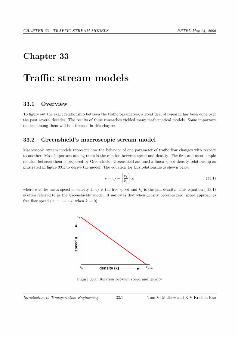
CHAPTER 33. TRAFFIC STREAM MODELS NPTEL May 24, 2006
Chapter 33
Traffic stream models
33.1 Overview
To figure out the exact relationship between the traffic parameters, a great deal of research has been done over
the past several decades. The results of these researches yielded many mathematical models. Some important
models among them will be discussed in this chapter.
33.2 Greenshield’s macroscopic stream model
Macroscopic stream models represent how the behavior of one parameter of traffic flow changes with respect
to another. Most important among them is the relation between speed and density. The first and most simple
relation between them is proposed by Greenshield. Greenshield assumed a linear speed-density relationship as
illustrated in figure 33:1 to derive the model. The equation for this relationship is shown below.
v = vf −
[
vf
kj
]
.k (33.1)
where v is the mean speed at density k, vf is the free speed and kj is the jam density. This equation ( 33.1)
is often referred to as the Greenshields’ model. It indicates that when density becomes zero, speed approaches
free flow speed (ie. v → vf when k → 0).
density (k)
spee
d u
kjam
uf
k0
Figure 33:1: Relation between speed and density
Introduction to Transportation Engineering 33.1 Tom V. Mathew and K V Krishna Rao
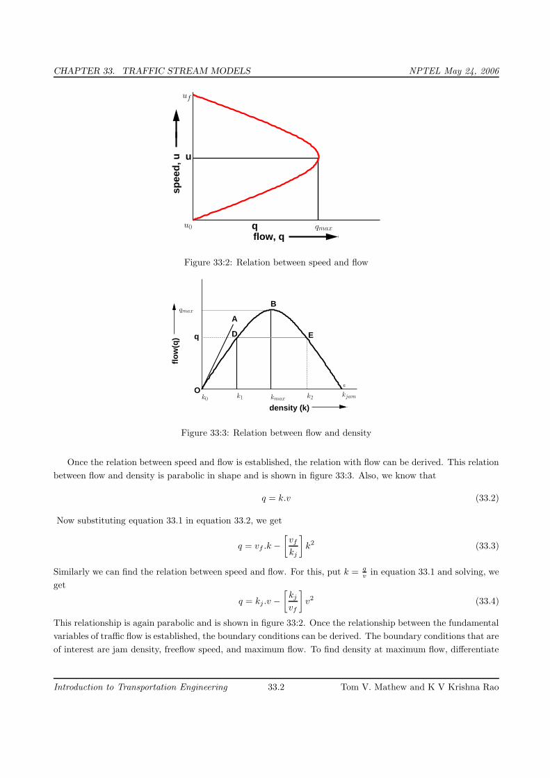
CHAPTER 33. TRAFFIC STREAM MODELS NPTEL May 24, 2006
spee
d, u u
flow, qq qmax
uf
u0
Figure 33:2: Relation between speed and flow
flo
w(q
)
C
B
A
q
O
density (k)
ED
qmax
k0k1 kmax k2
kjam
Figure 33:3: Relation between flow and density
Once the relation between speed and flow is established, the relation with flow can be derived. This relation
between flow and density is parabolic in shape and is shown in figure 33:3. Also, we know that
q = k.v (33.2)
Now substituting equation 33.1 in equation 33.2, we get
q = vf .k −
[
vf
kj
]
k2 (33.3)
Similarly we can find the relation between speed and flow. For this, put k = q
vin equation 33.1 and solving, we
get
q = kj .v −
[
kj
vf
]
v2 (33.4)
This relationship is again parabolic and is shown in figure 33:2. Once the relationship between the fundamental
variables of traffic flow is established, the boundary conditions can be derived. The boundary conditions that are
of interest are jam density, freeflow speed, and maximum flow. To find density at maximum flow, differentiate
Introduction to Transportation Engineering 33.2 Tom V. Mathew and K V Krishna Rao
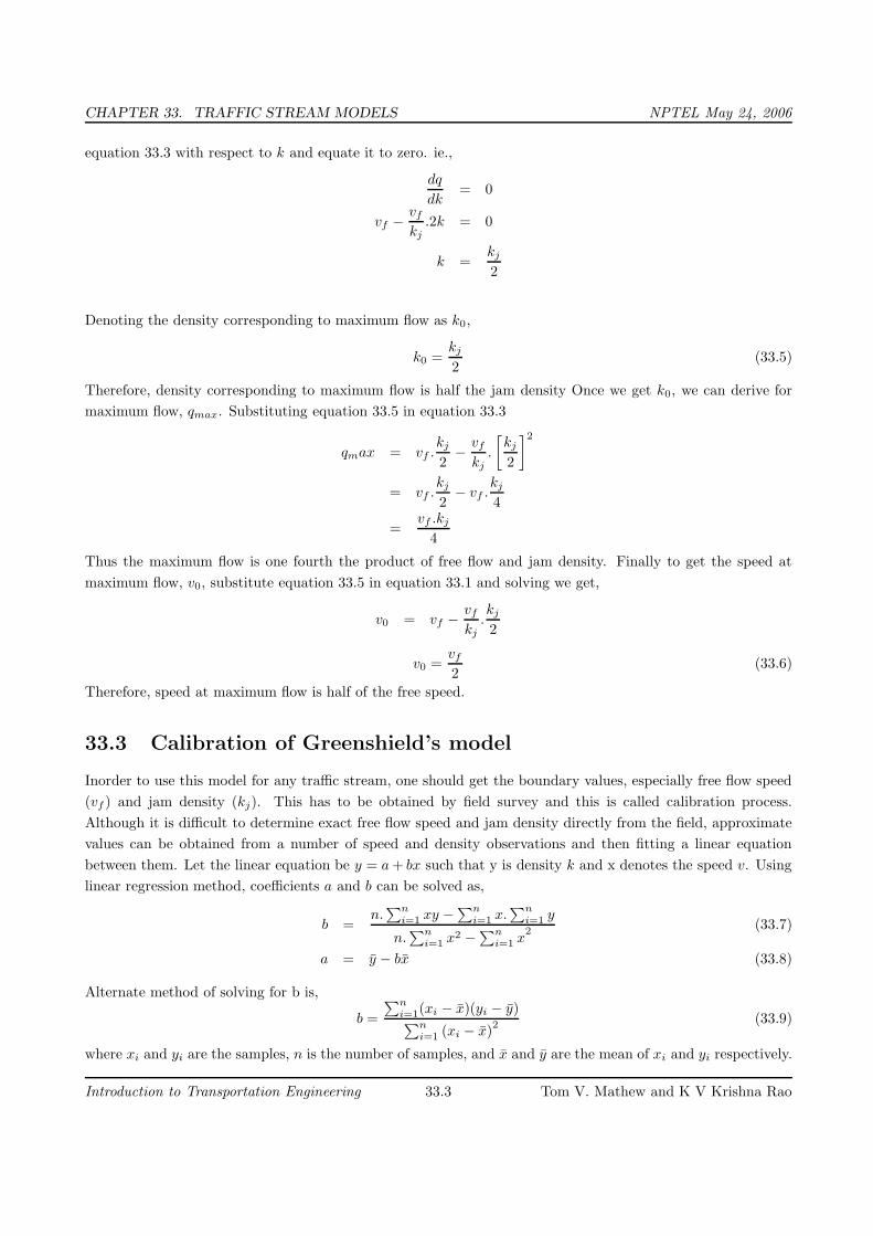
CHAPTER 33. TRAFFIC STREAM MODELS NPTEL May 24, 2006
equation 33.3 with respect to k and equate it to zero. ie.,
dq
dk= 0
vf −vf
kj
.2k = 0
k =kj
2
Denoting the density corresponding to maximum flow as k0,
k0 =kj
2(33.5)
Therefore, density corresponding to maximum flow is half the jam density Once we get k0, we can derive for
maximum flow, qmax. Substituting equation 33.5 in equation 33.3
qmax = vf .kj
2−
vf
kj
.
[
kj
2
]2
= vf .kj
2− vf .
kj
4
=vf .kj
4
Thus the maximum flow is one fourth the product of free flow and jam density. Finally to get the speed at
maximum flow, v0, substitute equation 33.5 in equation 33.1 and solving we get,
v0 = vf −vf
kj
.kj
2
v0 =vf
2(33.6)
Therefore, speed at maximum flow is half of the free speed.
33.3 Calibration of Greenshield’s model
Inorder to use this model for any traffic stream, one should get the boundary values, especially free flow speed
(vf ) and jam density (kj). This has to be obtained by field survey and this is called calibration process.
Although it is difficult to determine exact free flow speed and jam density directly from the field, approximate
values can be obtained from a number of speed and density observations and then fitting a linear equation
between them. Let the linear equation be y = a + bx such that y is density k and x denotes the speed v. Using
linear regression method, coefficients a and b can be solved as,
b =n.
∑n
i=1xy −
∑n
i=1x.
∑n
i=1y
n.∑n
i=1x2 −
∑n
i=1x
2(33.7)
a = y − bx (33.8)
Alternate method of solving for b is,
b =
∑
n
i=1(xi − x)(yi − y)
∑n
i=1(xi − x)
2(33.9)
where xi and yi are the samples, n is the number of samples, and x and y are the mean of xi and yi respectively.
Introduction to Transportation Engineering 33.3 Tom V. Mathew and K V Krishna Rao
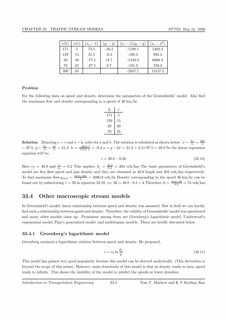
CHAPTER 33. TRAFFIC STREAM MODELS NPTEL May 24, 2006
x(k) y(v) (xi − x) (yi − y) (xi − x)(yi − y) (xi − x2)
171 5 73.5 -16.3 -1198.1 5402.3
129 15 31.5 -6.3 -198.5 992.3
20 40 -77.5 18.7 -1449.3 6006.3
70 25 -27.5 3.7 -101.8 756.3
390 85 -2947.7 13157.2
Problem
For the following data on speed and density, determine the parameters of the Greenshields’ model. Also find
the maximum flow and density corresponding to a speed of 30 km/hr.
k v
171 5
129 15
20 40
70 25
Solution Denoting y = v and x = k, solve for a and b .The solution is tabulated as shown below. x = Σx
n= 390
4
= 97.5, y = Σy
n= 85
4= 21.3. b = −2947.7
13157.2= -0.2 a = y − bx = 21.3 + 0.2×97.5 = 40.8 So the linear regression
equation will be,
v = 40.8− 0.2k (33.10)
Here vf = 40.8 andvf
kj
= 0.2 This implies, kj = 40.8
0.2= 204 veh/km The basic parameters of Greenshield’s
model are free flow speed and jam density and they are obtained as 40.8 kmph and 204 veh/km respectively.
To find maximum flow,qmax = 40.8×204
4= 2080.8 veh/hr Density corresponding to the speed 30 km/hr can be
found out by substituting v = 30 in equation 33.10. i.e, 30 = 40.8 - 0.2 × k Therefore, k = 40.8−30
0.2= 54 veh/km
33.4 Other macroscopic stream models
In Greenshield’s model, linear relationship between speed and density was assumed. But in field we can hardly
find such a relationship between speed and density. Therefore, the validity of Greenshields’ model was questioned
and many other models came up. Prominent among them are Greenberg’s logarithmic model, Underwood’s
exponential model, Pipe’s generalized model, and multiregime models. These are briefly discussed below.
33.4.1 Greenberg’s logarithmic model
Greenberg assumed a logarithmic relation between speed and density. He proposed,
v = v0 lnkj
k(33.11)
This model has gained very good popularity because this model can be derived analytically. (This derivation is
beyond the scope of this notes). However, main drawbacks of this model is that as density tends to zero, speed
tends to infinity. This shows the inability of the model to predict the speeds at lower densities.
Introduction to Transportation Engineering 33.4 Tom V. Mathew and K V Krishna Rao
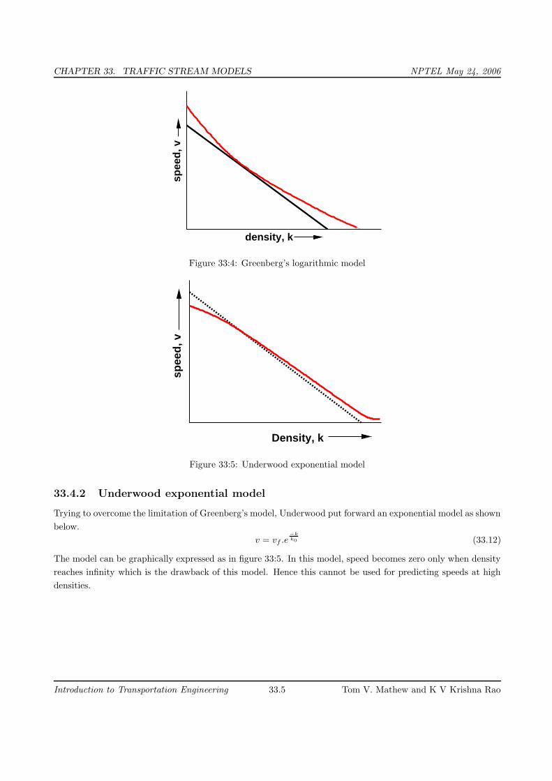
CHAPTER 33. TRAFFIC STREAM MODELS NPTEL May 24, 2006
density, k
spee
d, v
Figure 33:4: Greenberg’s logarithmic model
spee
d, v
Density, k
Figure 33:5: Underwood exponential model
33.4.2 Underwood exponential model
Trying to overcome the limitation of Greenberg’s model, Underwood put forward an exponential model as shown
below.
v = vf .e−k
k0 (33.12)
The model can be graphically expressed as in figure 33:5. In this model, speed becomes zero only when density
reaches infinity which is the drawback of this model. Hence this cannot be used for predicting speeds at high
densities.
Introduction to Transportation Engineering 33.5 Tom V. Mathew and K V Krishna Rao
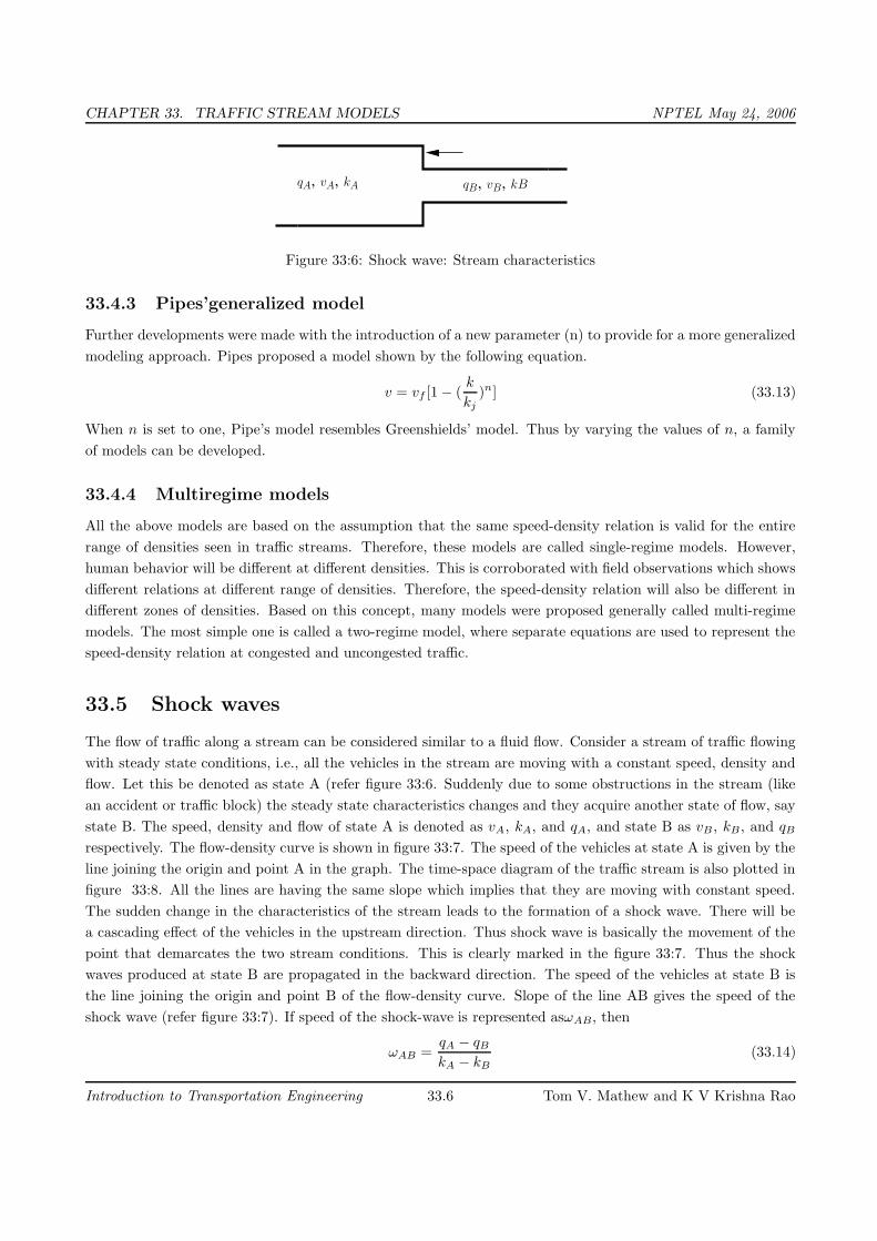
CHAPTER 33. TRAFFIC STREAM MODELS NPTEL May 24, 2006
qA, vA, kA qB, vB, kB
Figure 33:6: Shock wave: Stream characteristics
33.4.3 Pipes’generalized model
Further developments were made with the introduction of a new parameter (n) to provide for a more generalized
modeling approach. Pipes proposed a model shown by the following equation.
v = vf [1 − (k
kj
)n] (33.13)
When n is set to one, Pipe’s model resembles Greenshields’ model. Thus by varying the values of n, a family
of models can be developed.
33.4.4 Multiregime models
All the above models are based on the assumption that the same speed-density relation is valid for the entire
range of densities seen in traffic streams. Therefore, these models are called single-regime models. However,
human behavior will be different at different densities. This is corroborated with field observations which shows
different relations at different range of densities. Therefore, the speed-density relation will also be different in
different zones of densities. Based on this concept, many models were proposed generally called multi-regime
models. The most simple one is called a two-regime model, where separate equations are used to represent the
speed-density relation at congested and uncongested traffic.
33.5 Shock waves
The flow of traffic along a stream can be considered similar to a fluid flow. Consider a stream of traffic flowing
with steady state conditions, i.e., all the vehicles in the stream are moving with a constant speed, density and
flow. Let this be denoted as state A (refer figure 33:6. Suddenly due to some obstructions in the stream (like
an accident or traffic block) the steady state characteristics changes and they acquire another state of flow, say
state B. The speed, density and flow of state A is denoted as vA, kA, and qA, and state B as vB , kB , and qB
respectively. The flow-density curve is shown in figure 33:7. The speed of the vehicles at state A is given by the
line joining the origin and point A in the graph. The time-space diagram of the traffic stream is also plotted in
figure 33:8. All the lines are having the same slope which implies that they are moving with constant speed.
The sudden change in the characteristics of the stream leads to the formation of a shock wave. There will be
a cascading effect of the vehicles in the upstream direction. Thus shock wave is basically the movement of the
point that demarcates the two stream conditions. This is clearly marked in the figure 33:7. Thus the shock
waves produced at state B are propagated in the backward direction. The speed of the vehicles at state B is
the line joining the origin and point B of the flow-density curve. Slope of the line AB gives the speed of the
shock wave (refer figure 33:7). If speed of the shock-wave is represented asωAB, then
ωAB =qA − qB
kA − kB
(33.14)
Introduction to Transportation Engineering 33.6 Tom V. Mathew and K V Krishna Rao
CHAPTER 33. TRAFFIC STREAM MODELS NPTEL May 24, 2006
density
A
B
flo
w
kjkBkA
qB
vA
vBqA
Figure 33:7: Shock wave: Flow-density curve
time
dis
tan
ce
AB
Figure 33:8: Shock wave : time-distance diagram
Introduction to Transportation Engineering 33.7 Tom V. Mathew and K V Krishna Rao
CHAPTER 33. TRAFFIC STREAM MODELS NPTEL May 24, 2006
There are possibilities for other types of shockwaves such as forward moving shockwaves and stationary
shockwaves. The forward moving shockwaves are formed when a stream with higher density and higher flow
meets a stream with relatively lesser density and flow. For example, when the width of the road increases
suddenly, there are chances for a forward moving shockwave. Stationary shockwaves will occur when two
streams having the same flow value but different densities meet.
33.6 Macroscopic flow models
If one looks into traffic flow from a very long distance, the flow of fairly heavy traffic appears like a stream
of a fluid. Therefore, a macroscopic theory of traffic can be developed with the help of hydrodynamic theory
of fluids by considering traffic as an effectively one-dimensional compressible fluid. The behavior of individual
vehicle is ignored and one is concerned only with the behavior of sizable aggregate of vehicles. The earliest
traffic flow models began by writing the balance equation to address vehicle number conservation on a road.
Infact, all traffic flow models and theories must satisfy the law of conservation of the number of vehicles on the
road. Assuming that the vehicles are flowing from left to right, the continuity equation can be written as
∂k(x, t)
∂t+
∂q(x, t)
∂x= 0 (33.15)
where x denotes the spatial coordinate in the direction of traffic flow, t is the time, k is the density and q denotes
the flow. However, one cannot get two unknowns, namely k(x, t) by and q(x, t) by solving one equation. One
possible solution is to write two equations from two regimes of the flow, say before and after a bottleneck. In
this system the flow rate before and after will be same, or
k1v1 = k2v2 (33.16)
From this the shockwave velocity can be derived as
v(to)p =q2 − q1
k2 − k1
(33.17)
This is normally referred to as Stock’s shockwave formula. An alternate possibility which Lighthill and Whitham
adopted in their landmark study is to assume that the flow rate q is determined primarily by the local density
k, so that flow q can be treated as a function of only density k. Therefore the number of unknown variables
will be reduced to one. Essentially this assumption states that k(x,t) and q (x,t) are not independent of each
other. Therefore the continuity equation takes the form
∂k(x, t)
∂t+
∂q(k(x, t))
∂x= 0 (33.18)
However, the functional relationship between flow q and density k cannot be calculated from fluid-dynamical
theory. This has to be either taken as a phenomenological relation derived from the empirical observation or
from microscopic theories. Therefore, the flow rate q is a function of the vehicular density k; q = q(k). Thus,
the balance equation takes the form∂k(x, t)
∂t+
∂q(k(x, t))
∂x= 0 (33.19)
Now there is only one independent variable in the balance equation, the vehicle density k. If initial and
boundary conditions are known, this can be solved. Solution to LWR models are kinematic waves moving with
velocitydq(k)
dk(33.20)
Introduction to Transportation Engineering 33.8 Tom V. Mathew and K V Krishna Rao
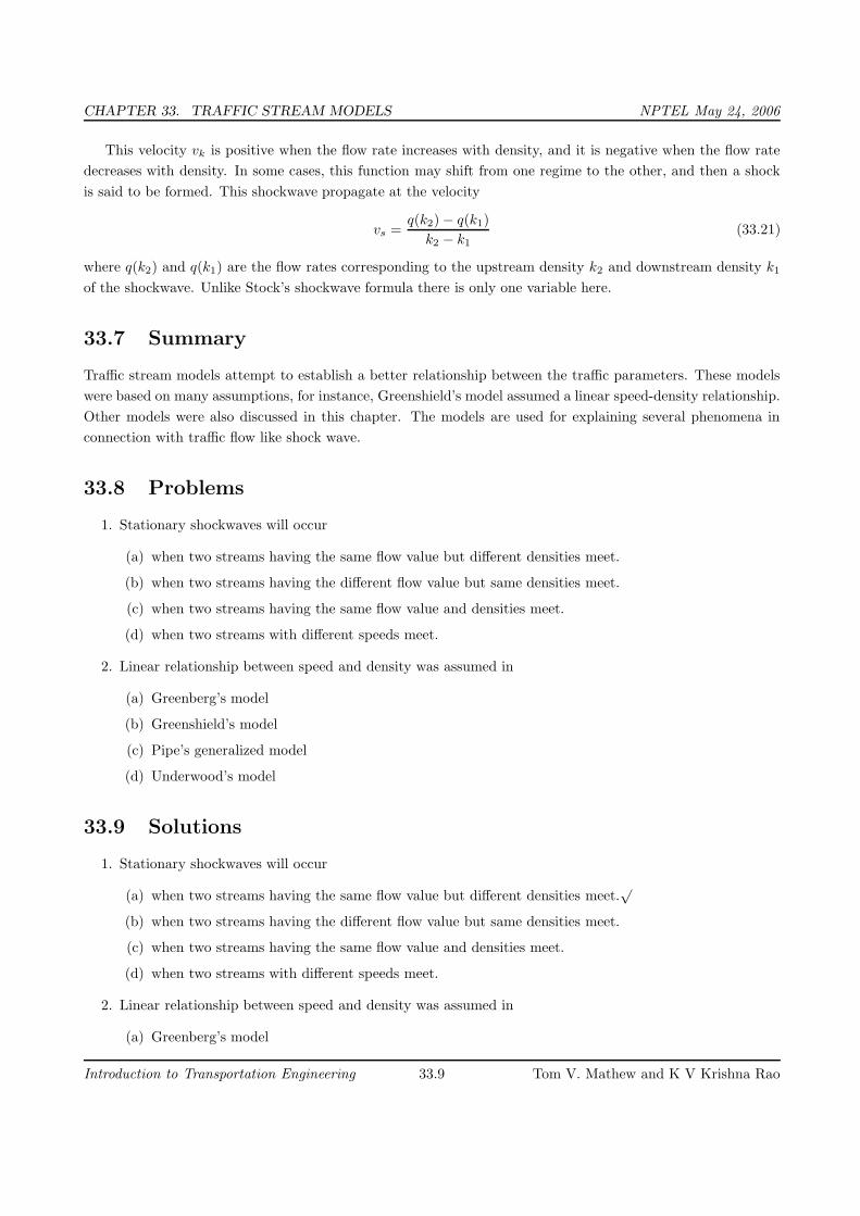
CHAPTER 33. TRAFFIC STREAM MODELS NPTEL May 24, 2006
This velocity vk is positive when the flow rate increases with density, and it is negative when the flow rate
decreases with density. In some cases, this function may shift from one regime to the other, and then a shock
is said to be formed. This shockwave propagate at the velocity
vs =q(k2) − q(k1)
k2 − k1
(33.21)
where q(k2) and q(k1) are the flow rates corresponding to the upstream density k2 and downstream density k1
of the shockwave. Unlike Stock’s shockwave formula there is only one variable here.
33.7 Summary
Traffic stream models attempt to establish a better relationship between the traffic parameters. These models
were based on many assumptions, for instance, Greenshield’s model assumed a linear speed-density relationship.
Other models were also discussed in this chapter. The models are used for explaining several phenomena in
connection with traffic flow like shock wave.
33.8 Problems
1. Stationary shockwaves will occur
(a) when two streams having the same flow value but different densities meet.
(b) when two streams having the different flow value but same densities meet.
(c) when two streams having the same flow value and densities meet.
(d) when two streams with different speeds meet.
2. Linear relationship between speed and density was assumed in
(a) Greenberg’s model
(b) Greenshield’s model
(c) Pipe’s generalized model
(d) Underwood’s model
33.9 Solutions
1. Stationary shockwaves will occur
(a) when two streams having the same flow value but different densities meet.√
(b) when two streams having the different flow value but same densities meet.
(c) when two streams having the same flow value and densities meet.
(d) when two streams with different speeds meet.
2. Linear relationship between speed and density was assumed in
(a) Greenberg’s model
Introduction to Transportation Engineering 33.9 Tom V. Mathew and K V Krishna Rao
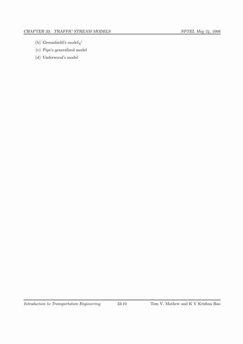
CHAPTER 33. TRAFFIC STREAM MODELS NPTEL May 24, 2006
(b) Greenshield’s model√
(c) Pipe’s generalized model
(d) Underwood’s model
Introduction to Transportation Engineering 33.10 Tom V. Mathew and K V Krishna Rao
CHAPTER 34. MICROSCOPIC TRAFFIC FLOW MODELING NPTEL May 24, 2006
Chapter 34
Microscopic traffic flow modeling
34.1 Overview
Macroscopic modeling looks at traffic flow from a global perspective, whereas microscopic modeling, as the term
suggests, gives attention to the details of traffic flow and the interactions taking place within it. This chapter
gives an overview of microscopic approach to modeling traffic and then elaborates on the various concepts
associated with it.
A microscopic model of traffic flow attempts to analyze the flow of traffic by modeling driver-driver and
driver-road interactions within a traffic stream which respectively analyzes the interaction between a driver and
another driver on road and of a single driver on the different features of a road. Many studies and researches
were carried out on driver’s behavior in different situations like a case when he meets a static obstacle or when
he meets a dynamic obstacle. Several studies are made on modeling driver behavior in another following car
and such studies are often referred to as car following theories of vehicular traffic.
34.2 Notation
Longitudinal spacing of vehicles are of particular importance from the points of view of safety, capacity and
level of service. The longitudinal space occupied by a vehicle depend on the physical dimensions of the vehicles
as well as the gaps between vehicles. For measuring this longitudinal space, two microscopic measures are used-
distance headway and distance gap. Distance headway is defined as the distance from a selected point (usually
front bumper) on the lead vehicle to the corresponding point on the following vehicles. Hence, it includes the
length of the lead vehicle and the gap length between the lead and the following vehicles. Before going in to
the details, various notations used in car-following models are discussed here with the help of figure 34:1. The
leader vehicle is denoted as n and the following vehicle as (n + 1). Two characteristics at an instant t are of
importance; location and speed. Location and speed of the lead vehicle at time instant t are represented by xtn
and vtn respectively. Similarly, the location and speed of the follower are denoted by xt
n+1and vt
n+1respectively.
The following vehicle is assumed to accelerate at time t + ∆T and not at t, where ∆T is the interval of time
required for a driver to react to a changing situation. The gap between the leader and the follower vehicle is
therefore xtn − xt
n+1.
Introduction to Transportation Engineering 34.1 Tom V. Mathew and K V Krishna Rao
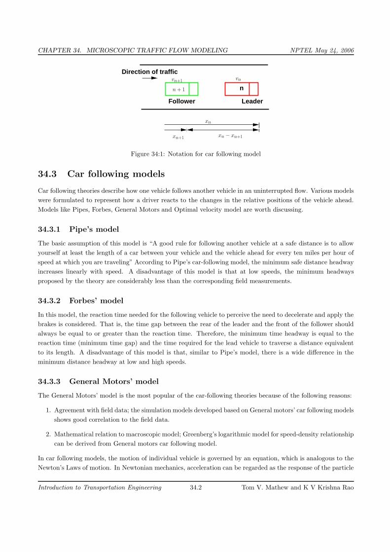
CHAPTER 34. MICROSCOPIC TRAFFIC FLOW MODELING NPTEL May 24, 2006
Follower
Direction of traffic
Leader
nvn+1
n + 1
vn
xn − xn+1
xn
xn+1
Figure 34:1: Notation for car following model
34.3 Car following models
Car following theories describe how one vehicle follows another vehicle in an uninterrupted flow. Various models
were formulated to represent how a driver reacts to the changes in the relative positions of the vehicle ahead.
Models like Pipes, Forbes, General Motors and Optimal velocity model are worth discussing.
34.3.1 Pipe’s model
The basic assumption of this model is “A good rule for following another vehicle at a safe distance is to allow
yourself at least the length of a car between your vehicle and the vehicle ahead for every ten miles per hour of
speed at which you are traveling” According to Pipe’s car-following model, the minimum safe distance headway
increases linearly with speed. A disadvantage of this model is that at low speeds, the minimum headways
proposed by the theory are considerably less than the corresponding field measurements.
34.3.2 Forbes’ model
In this model, the reaction time needed for the following vehicle to perceive the need to decelerate and apply the
brakes is considered. That is, the time gap between the rear of the leader and the front of the follower should
always be equal to or greater than the reaction time. Therefore, the minimum time headway is equal to the
reaction time (minimum time gap) and the time required for the lead vehicle to traverse a distance equivalent
to its length. A disadvantage of this model is that, similar to Pipe’s model, there is a wide difference in the
minimum distance headway at low and high speeds.
34.3.3 General Motors’ model
The General Motors’ model is the most popular of the car-following theories because of the following reasons:
1. Agreement with field data; the simulation models developed based on General motors’ car following models
shows good correlation to the field data.
2. Mathematical relation to macroscopic model; Greenberg’s logarithmic model for speed-density relationship
can be derived from General motors car following model.
In car following models, the motion of individual vehicle is governed by an equation, which is analogous to the
Newton’s Laws of motion. In Newtonian mechanics, acceleration can be regarded as the response of the particle
Introduction to Transportation Engineering 34.2 Tom V. Mathew and K V Krishna Rao
CHAPTER 34. MICROSCOPIC TRAFFIC FLOW MODELING NPTEL May 24, 2006
to stimulus it receives in the form of force which includes both the external force as well as those arising from
the interaction with all other particles in the system. This model is the widely used and will be discussed in
detail later.
34.3.4 Optimal velocity model
The concept of this model is that each driver tries to achieve an optimal velocity based on the distance to the
preceding vehicle and the speed difference between the vehicles. This was an alternative possibility explored
recently in car-following models. The formulation is based on the assumption that the desired speed vndesired
depends on the distance headway of the nth vehicle. i.e.vtndesired
= vopt(∆xtn) where vopt is the optimal velocity
function which is a function of the instantaneous distance headway ∆xtn. Therefore at
nis given by
at
n= [1/τ ][V opt(∆xt
n) − vt
n] (34.1)
where 1
τis called as sensitivity coefficient. In short, the driving strategy of nth vehicle is that, it tries to maintain
a safe speed which inturn depends on the relative position, rather than relative speed.
34.4 General motor’s car following model
34.4.1 Basic Philosophy
The basic philosophy of car following model is from Newtonian mechanics, where the acceleration may be
regarded as the response of a matter to the stimulus it receives in the form of the force it receives from the
interaction with other particles in the system. Hence, the basic philosophy of car-following theories can be
summarized by the following equation
[Response]n α [Stimulus]n (34.2)
for the nth vehicle (n=1, 2, ...). Each driver can respond to the surrounding traffic conditions only by accelerating
or decelerating the vehicle. As mentioned earlier, different theories on car-following have arisen because of the
difference in views regarding the nature of the stimulus. The stimulus may be composed of the speed of the
vehicle, relative speeds, distance headway etc, and hence, it is not a single variable, but a function and can be
represented as,
at
n = fsti(vn, ∆xn, ∆vn) (34.3)
where fsti is the stimulus function that depends on the speed of the current vehicle, relative position and speed
with the front vehicle.
34.4.2 Follow-the-leader model
The car following model proposed by General motors is based on follow-the leader concept. This is based on
two assumptions; (a) higher the speed of the vehicle, higher will be the spacing between the vehicles and (b) to
avoid collision, driver must maintain a safe distance with the vehicle ahead.
Let ∆xtn+1
is the gap available for (n+1)th vehicle, and let ∆xsafe is the safe distance, vtn+1
and vtn
are the
velocities, the gap required is given by,
∆xt
n+1= ∆xsafe + τvt
n+1(34.4)
Introduction to Transportation Engineering 34.3 Tom V. Mathew and K V Krishna Rao
CHAPTER 34. MICROSCOPIC TRAFFIC FLOW MODELING NPTEL May 24, 2006
where τ is a sensitivity coefficient. The above equation can be written as
xn − xt
n+1= ∆xsafe + τvt
n+1(34.5)
Differentiating the above equation with respect to time, we get
vt
n − vt
n+1= τ.at
n+1
at
n+1=
1
τ[vt
n− vt
n+1]
General Motors has proposed various forms of sensitivity coefficient term resulting in five generations of models.
The most general model has the form,
at
n+1=
[
αl,m(vtn+1
)m
(xtn − xt
n+1)l
]
[
vt
n − vt
n+1] (34.6)
where l is a distance headway exponent and can take values from +4 to -1, m is a speed exponent and can take
values from -2 to +2, and α is a sensitivity coefficient. These parameters are to be calibrated using field data.
This equation is the core of traffic simulation models.
In computer, implementation of the simulation models, three things need to be remembered:
1. A driver will react to the change in speed of the front vehicle after a time gap called the reaction time
during which the follower perceives the change in speed and react to it.
2. The vehicle position, speed and acceleration will be updated at certain time intervals depending on the
accuracy required. Lower the time interval, higher the accuracy.
3. Vehicle position and speed is governed by Newton’s laws of motion, and the acceleration is governed by
the car following model.
Therefore, the governing equations of a traffic flow can be developed as below. Let ∆T is the reaction time,
and ∆t is the updation time, the governing equations can be written as,
vt
n = vt−∆t
n + at−∆t
n × ∆t (34.7)
xt
n = xt−∆t
n + vt−∆t
n × ∆t +1
2at−∆t
n ∆t2 (34.8)
at
n+1= [
αl,m(vt−∆T
n+1)
(xt−∆Tn − xt−∆T
n+1
][vt−∆T
n− vt−∆T
n+1] (34.9)
The equation 34.7 is a simulation version of the Newton’s simple law of motion v = u + at and equation 34.8
is the simulation version of the Newton’s another equation s = ut + 1
2at2. The acceleration of the follower
vehicle depends upon the relative velocity of the leader and the follower vehicle, sensitivity coefficient and the
gap between the vehicles.
Problem
Let a leader vehicle is moving with zero acceleration for two seconds from time zero. Then he accelerates by 1
m/s2 for 2 seconds, then decelerates by 1m/s2for 2 seconds. The initial speed is 16 m/s and initial location is
28 m from datum. A vehicle is following this vehicle with initial speed 16 m/s, and position zero. Simulate the
behavior of the following vehicle using General Motors’ Car following model (acceleration, speed and position)
for 7.5 seconds. Assume the parameters l=1, m=0 , sensitivity coefficient (αl,m) = 13, reaction time as 1 second
and scan interval as 0.5 seconds.
Introduction to Transportation Engineering 34.4 Tom V. Mathew and K V Krishna Rao
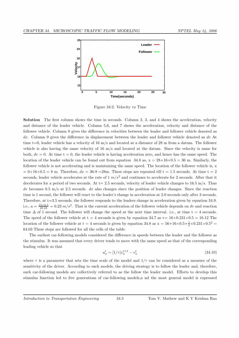
CHAPTER 34. MICROSCOPIC TRAFFIC FLOW MODELING NPTEL May 24, 2006
Follower
Leader
Time(seconds)
Vel
oci
ty
15 20 25 10 5 0
17
18
19
20
16
15
30
Figure 34:2: Velocity vz Time
Solution The first column shows the time in seconds. Column 2, 3, and 4 shows the acceleration, velocity
and distance of the leader vehicle. Column 5,6, and 7 shows the acceleration, velocity and distance of the
follower vehicle. Column 8 gives the difference in velocities between the leader and follower vehicle denoted as
dx. Column 9 gives the difference in displacement between the leader and follower vehicle denoted as dv At
time t=0, leader vehicle has a velocity of 16 m/s and located at a distance of 28 m from a datum. The follower
vehicle is also having the same velocity of 16 m/s and located at the datum. Since the velocity is same for
both, dv = 0. At time t = 0, the leader vehicle is having acceleration zero, and hence has the same speed. The
location of the leader vehicle can be found out from equation 34.8 as, x = 28+16×0.5 = 36 m. Similarly, the
follower vehicle is not accelerating and is maintaining the same speed. The location of the follower vehicle is, x
= 0+16×0.5 = 8 m. Therefore, dx = 36-8 =28m. These steps are repeated till t = 1.5 seconds. At time t = 2
seconds, leader vehicle accelerates at the rate of 1 m/s2 and continues to accelerate for 2 seconds. After that it
decelerates for a period of two seconds. At t= 2.5 seconds, velocity of leader vehicle changes to 16.5 m/s. Thus
dv becomes 0.5 m/s at 2.5 seconds. dx also changes since the position of leader changes. Since the reaction
time is 1 second, the follower will react to the leader’s change in acceleration at 2.0 seconds only after 3 seconds.
Therefore, at t=3.5 seconds, the follower responds to the leaders change in acceleration given by equation 34.9.
i.e., a = 13×0.5
28.23= 0.23 m/s2. That is the current acceleration of the follower vehicle depends on dv and reaction
time ∆ of 1 second. The follower will change the speed at the next time interval. i.e., at time t = 4 seconds.
The speed of the follower vehicle at t = 4 seconds is given by equation 34.7 as v= 16+0.231×0.5 = 16.12 The
location of the follower vehicle at t = 4 seconds is given by equation 34.8 as x = 56+16×0.5+ 1
2×0.231×0.52 =
64.03 These steps are followed for all the cells of the table.
The earliest car-following models considered the difference in speeds between the leader and the follower as
the stimulus. It was assumed that every driver tends to move with the same speed as that of the corresponding
leading vehicle so that
at
n = [1/τ ]vt+1
n − vt
n (34.10)
where τ is a parameter that sets the time scale of the model and 1/τ can be considered as a measure of the
sensitivity of the driver. According to such models, the driving strategy is to follow the leader and, therefore,
such car-following models are collectively referred to as the follow the leader model. Efforts to develop this
stimulus function led to five generations of car-following models,a nd the most general model is expressed
Introduction to Transportation Engineering 34.5 Tom V. Mathew and K V Krishna Rao
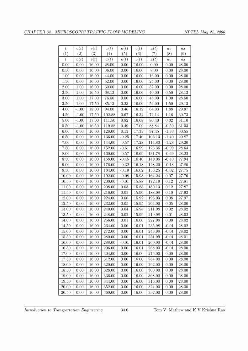
CHAPTER 34. MICROSCOPIC TRAFFIC FLOW MODELING NPTEL May 24, 2006
t a(t) v(t) x(t) a(t) v(t) x(t) dv dx
(1) (2) (3) (4) (5) (6) (7) (8) (9)
t a(t) v(t) x(t) a(t) v(t) x(t) dv dx
0.00 0.00 16.00 28.00 0.00 16.00 0.00 0.00 28.00
0.50 0.00 16.00 36.00 0.00 16.00 8.00 0.00 28.00
1.00 0.00 16.00 44.00 0.00 16.00 16.00 0.00 28.00
1.50 0.00 16.00 52.00 0.00 16.00 24.00 0.00 28.00
2.00 1.00 16.00 60.00 0.00 16.00 32.00 0.00 28.00
2.50 1.00 16.50 68.13 0.00 16.00 40.00 0.50 28.13
3.00 1.00 17.00 76.50 0.00 16.00 48.00 1.00 28.50
3.50 1.00 17.50 85.13 0.23 16.00 56.00 1.50 29.13
4.00 -1.00 18.00 94.00 0.46 16.12 64.03 1.88 29.97
4.50 -1.00 17.50 102.88 0.67 16.34 72.14 1.16 30.73
5.00 -1.00 17.00 111.50 0.82 16.68 80.40 0.32 31.10
5.50 -1.00 16.50 119.88 0.49 17.09 88.84 -0.59 31.03
6.00 0.00 16.00 128.00 0.13 17.33 97.45 -1.33 30.55
6.50 0.00 16.00 136.00 -0.25 17.40 106.13 -1.40 29.87
7.00 0.00 16.00 144.00 -0.57 17.28 114.80 -1.28 29.20
7.50 0.00 16.00 152.00 -0.61 16.99 123.36 -0.99 28.64
8.00 0.00 16.00 160.00 -0.57 16.69 131.78 -0.69 28.22
8.50 0.00 16.00 168.00 -0.45 16.40 140.06 -0.40 27.94
9.00 0.00 16.00 176.00 -0.32 16.18 148.20 -0.18 27.80
9.50 0.00 16.00 184.00 -0.19 16.02 156.25 -0.02 27.75
10.00 0.00 16.00 192.00 -0.08 15.93 164.24 0.07 27.76
10.50 0.00 16.00 200.00 -0.01 15.88 172.19 0.12 27.81
11.00 0.00 16.00 208.00 0.03 15.88 180.13 0.12 27.87
11.50 0.00 16.00 216.00 0.05 15.90 188.08 0.10 27.92
12.00 0.00 16.00 224.00 0.06 15.92 196.03 0.08 27.97
12.50 0.00 16.00 232.00 0.05 15.95 204.00 0.05 28.00
13.00 0.00 16.00 240.00 0.04 15.98 211.98 0.02 28.02
13.50 0.00 16.00 248.00 0.02 15.99 219.98 0.01 28.02
14.00 0.00 16.00 256.00 0.01 16.00 227.98 0.00 28.02
14.50 0.00 16.00 264.00 0.00 16.01 235.98 -0.01 28.02
15.00 0.00 16.00 272.00 0.00 16.01 243.98 -0.01 28.02
15.50 0.00 16.00 280.00 0.00 16.01 251.99 -0.01 28.01
16.00 0.00 16.00 288.00 -0.01 16.01 260.00 -0.01 28.00
16.50 0.00 16.00 296.00 0.00 16.01 268.00 -0.01 28.00
17.00 0.00 16.00 304.00 0.00 16.00 276.00 0.00 28.00
17.50 0.00 16.00 312.00 0.00 16.00 284.00 0.00 28.00
18.00 0.00 16.00 320.00 0.00 16.00 292.00 0.00 28.00
18.50 0.00 16.00 328.00 0.00 16.00 300.00 0.00 28.00
19.00 0.00 16.00 336.00 0.00 16.00 308.00 0.00 28.00
19.50 0.00 16.00 344.00 0.00 16.00 316.00 0.00 28.00
20.00 0.00 16.00 352.00 0.00 16.00 324.00 0.00 28.00
20.50 0.00 16.00 360.00 0.00 16.00 332.00 0.00 28.00
Introduction to Transportation Engineering 34.6 Tom V. Mathew and K V Krishna Rao
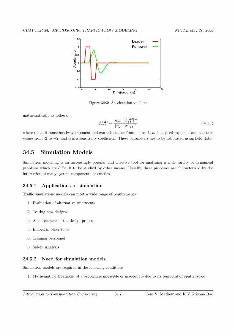
CHAPTER 34. MICROSCOPIC TRAFFIC FLOW MODELING NPTEL May 24, 2006
FollowerLeader
25 20 15 10 5 0
−0.5
−1
0
0.5
1
1.5
−1.5 30
Time(seconds)
Acc
eler
atio
n
Figure 34:3: Acceleration vz Time
mathematically as follows.
qt+∆t
n+1=
αl,m [vt+∆t
n+1]m
[xtn− xt
n+1]l
(34.11)
where l is a distance headway exponent and can take values from +4 to -1, m is a speed exponent and can take
values from -2 to +2, and α is a sensitivity coefficient. These parameters are to be calibrated using field data.
34.5 Simulation Models
Simulation modeling is an increasingly popular and effective tool for analyzing a wide variety of dynamical
problems which are difficult to be studied by other means. Usually, these processes are characterized by the
interaction of many system components or entities.
34.5.1 Applications of simulation
Traffic simulations models can meet a wide range of requirements:
1. Evaluation of alternative treatments
2. Testing new designs
3. As an element of the design process
4. Embed in other tools
5. Training personnel
6. Safety Analysis
34.5.2 Need for simulation models
Simulation models are required in the following conditions
1. Mathematical treatment of a problem is infeasible or inadequate due to its temporal or spatial scale
Introduction to Transportation Engineering 34.7 Tom V. Mathew and K V Krishna Rao
CHAPTER 34. MICROSCOPIC TRAFFIC FLOW MODELING NPTEL May 24, 2006
2. The accuracy or applicability of the results of a mathematical formulation is doubtful, because of the
assumptions underlying (e.g., a linear program) or an heuristic procedure (e.g., those in the Highway
Capacity Manual)
3. The mathematical formulation represents the dynamic traffic/control environment as a simpler quasi
steady state system.
4. There is a need to view vehicle animation displays to gain an understanding of how the system is behaving
5. Training personnel
6. Congested conditions persist over a significant time.
34.5.3 Classification of Simulation Model
Simulation models are classified based on many factors like
1. Continuity
(a) Continuous model
(b) Discrete model
2. Level of detail
(a) Macroscopic models
(b) Mesoscopic models
(c) Microscopic models
3. Based on Processes
(a) Deterministic
(b) Stochastic
34.6 Summary
Microscopic traffic flow modeling focuses on the minute aspects of traffic stream like vehicle to vehicle interaction
and individual vehicle behavior. They help to analyze very small changes in the traffic stream over time and
space. Car following model is one such model where in the stimulus-response concept is employed. Optimal
models and simulation models were briefly discussed.
34.7 Problems
1. The minimum safe distance headway increases linearly with speed. Which model follows this assumption?
(a) Forbe’s model
(b) Pipe’s model
(c) General motor’s model
Introduction to Transportation Engineering 34.8 Tom V. Mathew and K V Krishna Rao
CHAPTER 34. MICROSCOPIC TRAFFIC FLOW MODELING NPTEL May 24, 2006
(d) Optimal velocity model
2. The most popular of the car following models is
(a) Forbe’s model
(b) Pipe’s model
(c) General motor’s model
(d) Optimal velocity model
34.8 Solutions
1. The minimum safe distance headway increases linearly with speed. Which model follows this assumption?
(a) Forbe’s model
(b) Pipe’s model√
(c) General motor’s model
(d) Optimal velocity model
2. The most popular of the car following models is
(a) Forbe’s model
(b) Pipe’s model
(c) General motor’s model√
(d) Optimal velocity model
Introduction to Transportation Engineering 34.9 Tom V. Mathew and K V Krishna Rao
CHAPTER 35. CAPACITY AND LEVEL OF SERVICE NPTEL May 24, 2006
Chapter 35
Capacity and Level of service
35.1 Overview
Capacity and Level of service are two related terms. Capacity analysis tries to give a clear understanding of
how much traffic a given transportation facility can accommodate. Level of service tries to answer how good is
the present traffic situation on a given facility. Thus it gives a qualitative measure of traffic, where as capacity
analysis gives a quantitative measure of a facility. Capacity and level of service varies with the type of facility,
prevailing traffic and road conditions etc. These concepts are discussed in this chapter.
35.2 Capacity
Capacity is defined as the maximum number of vehicles, passengers, or the like, per unit time, which can be
accommodated under given conditions with a reasonable expectation of occurrence. Some of the observations
that are found from this definition can be now discussed. Capacity is independent of the demand. It speaks
about the physical amount of vehicles and passengers a road can afford. It does not depend on the total number
of vehicles demanding service. On the other hand, it depends on traffic conditions, geometric design of the road
etc. For example, a curved road has lesser capacity compared to a straight road. Capacity is expressed in terms
of units of some specific thing (car, people, etc.), so it also does depend on the traffic composition. In addition,
the capacity analysis depends on the environmental conditions too. Capacity is a probabilistic measure. It
varies with respect to time and position in the maximum number of units of demand it can accommodate by
similar facilities. Hence it is not always possible to completely derive analytically the capacity. In most cases it
is obtained, through field observations.
35.3 Level of service
A term closely related to capacity and often confused with it is service volume. When capacity gives a quan-
titative measure of traffic, level of service or LOS tries to give a qualitative measure. A service volume is the
maximum number of vehicles, passengers, or the like, which can be accommodated by a given facility or system
under given conditions at a given level of service.
For a given road or facility, capacity could be constant. But actual flow will be different for different days
and different times in a day itself. The intention of LOS is to relate the traffic service quality to a given flow rate
of traffic. It is a term that designates a range of operating conditions on a particular type of facility. Highway
capacity manual (HCM) developed by the transportation research board of USA provides some procedure to
Introduction to Transportation Engineering 35.1 Tom V. Mathew and K V Krishna Rao
CHAPTER 35. CAPACITY AND LEVEL OF SERVICE NPTEL May 24, 2006
determine level of service. It divides the quality of traffic into six levels ranging form level A to level F. Level
A represents the best quality of traffic where the driver has the freedom to drive with free flow speed and level
F represents the worst quality of traffic. Level of service is defined based on the measure of effectiveness or
(MOE). Typically three parameters are used under this and they are speed and travel time, density, and delay.
One of the important measures of service quality is the amount of time spent in travel. Therefore, speed and
travel time are considered to be more effective in defining LOS of a facility. Density gives the proximity of other
vehicles in the stream. Since it affects the ability of the driver to maneuver in the traffic stream, it is also used
to describe LOS. Delay is a term that describes excess or unexpected time spent in travel. Many specific delay
measures are defined and used as MOE’s in the highway capacity manual.
35.4 Types of facilities
Most important classification of transportation facilities from the engineering perspective is based on the conti-
nuity of flow, that is uninterrupted flow and interrupted flow. Uninterrupted flow is the flow of traffic in which
there is no obstructions to the movement of vehicles along the road. Freeway is one example for this type of
facility. In a freeway, when a vehicle enters a freeway, there is no need for the vehicle to stop anywhere till
it leaves the freeway. There are three sections in a freeway - basic unit, weaving section and ramps(on/off).
Vehicles will be entering the freeway through ramps. Ramps used for entering the freeway is called on-ramps
and those used for exiting the freeway are called off-ramps. Freeways generally have 4, 6, or 8 lane alignments.
Multi lanes also provide uninterrupted flow. In many roads, there will be signalized as well as unsignalized
intersections. Uninterrupted flow is possible in sections of rural and suburban multilane highways between
signalized intersections where signal spacing is sufficient to allow for uninterrupted flow. Two lane highways
also provide uninterrupted flow facilities.
Interrupted flow refers to the condition when the traffic flow on the road is obstructed due to some reasons.
This is experienced in signalized intersections, unsignalized intersections, arterials etc. At signalized intersec-
tions, there will be some kind of active control and the vehicle will have to stop or sometimes to reduce its
speed and the flow of traffic is interrupted. Thus the capacity is defined in terms of control delay ie sec/veh.
Arterials are roads of long stretches with many intersections in between and obviously there will be interruption
to the flow of traffic. Here, the capacity is expressed in terms of average travel speed. Some other facilities
are facilities for pedestrians, bicycles, bus-transit, rail-transit etc. Example for pedestrian facility is a provision
of subway exclusively for the use of pedestrians. Here, the capacity may be expressed in terms of number of
passengers. In bus transit system, the buses has to stop at the bus bays and also it has to share the road with
the other vehicles. Hence the capacity will be affected by the control characteristics and the traffic conditions
prevailing in the road. Since trains have exclusive right of way, the capacity is strictly governed by the control
characteristics. It has two types of capacities - line capacity and station capacity. Line capacity is based on
the number of tracks available between two stations. Station capacity refers to the facilities available in the
platform of the station,and other facilities.
For uninterrupted flow of traffic, measure of effectiveness (MOE) is density in freeways. Speed also becomes
important in two-lane highways and multilane highways. In the case of interrupted flow, MOE is delay. The
delay of travel time becomes an important factor in calculating the capacity.
Introduction to Transportation Engineering 35.2 Tom V. Mathew and K V Krishna Rao
CHAPTER 35. CAPACITY AND LEVEL OF SERVICE NPTEL May 24, 2006
35.5 Highway capacity
Highway capacity is defined by the Highway Capacity Manual as the maximum hourly rate at which persons
or vehicles can be reasonably expected to traverse a point or a uniform segment of a lane or roadway during a
given time period under prevailing roadway, traffic and control conditions. The highway capacity depends on
certain conditions as listed below;
1. Traffic conditions: It refers to the traffic composition in the road such as the mix of cars, trucks,
buses etc in the stream. It also include peaking characteristics, proportions of turning movements at
intersections etc.
2. Road way characteristics: This points out to the geometric characteristics of the road. These include
lane width, shoulder width, lane configuration, horizontal alignment and vertical alignment.
3. Control conditions: This primarily applies to surface facilities and often refer to the signals at inter-
sections etc.
Again capacity can be defined for a point or uniform section. Capacity is estimated for segments having
uniform conditions. Points where these conditions change represent the boundaries where separate analysis
may be required. Capacity is the maximum flow rate that a facility can afford. This maximum flow rate is
taken for the worst 15 minutes of the peak hours while finding out the capacity. Capacity is measured as a
reasonably expected value and not the maximum flow rate ever observed in the facility. This is because the
measured capacity at a single location will show significant variation from day to day. Further, local driving
habits also produce variations in the observed capacity.
35.6 Factors affecting level of service
level of service one can derive from a road under different operating characteristics and traffic volumes. The
factors affecting level of service (LOS) can be listed as follows:
1. Speed and travel time
2. Traffic interruptions/restrictions
3. Freedom to travel with desired speed
4. Driver comfort and convenience
5. Operating cost.
Highway Capacity Manual(HCM) used travel speed and volume by capacity ratio (v/c ratio) to distinguish
between various levels of service. The value of v/c ratio can vary between 0 and 1. Depending upon the
travel speed and v/c ratio, HCM has defined six levels of service, level A to level F based on a graph between
operating speed and v/c ratio as shown in the figure 35:1. Level of service A represents the zone of free flow.
Here the traffic volume will be less, traffic will be experiencing free flow also. The drivers will be having the
complete freedom to choose their desired speed. Even at maximum density, for this LOS the average spacing
between vehicles is 167 m. Lane changes within the traffic stream, as well as merging and diverging movements,
are made relatively easy. The effect of minor incidents and point breakdowns are easily aborted at this level.
Introduction to Transportation Engineering 35.3 Tom V. Mathew and K V Krishna Rao
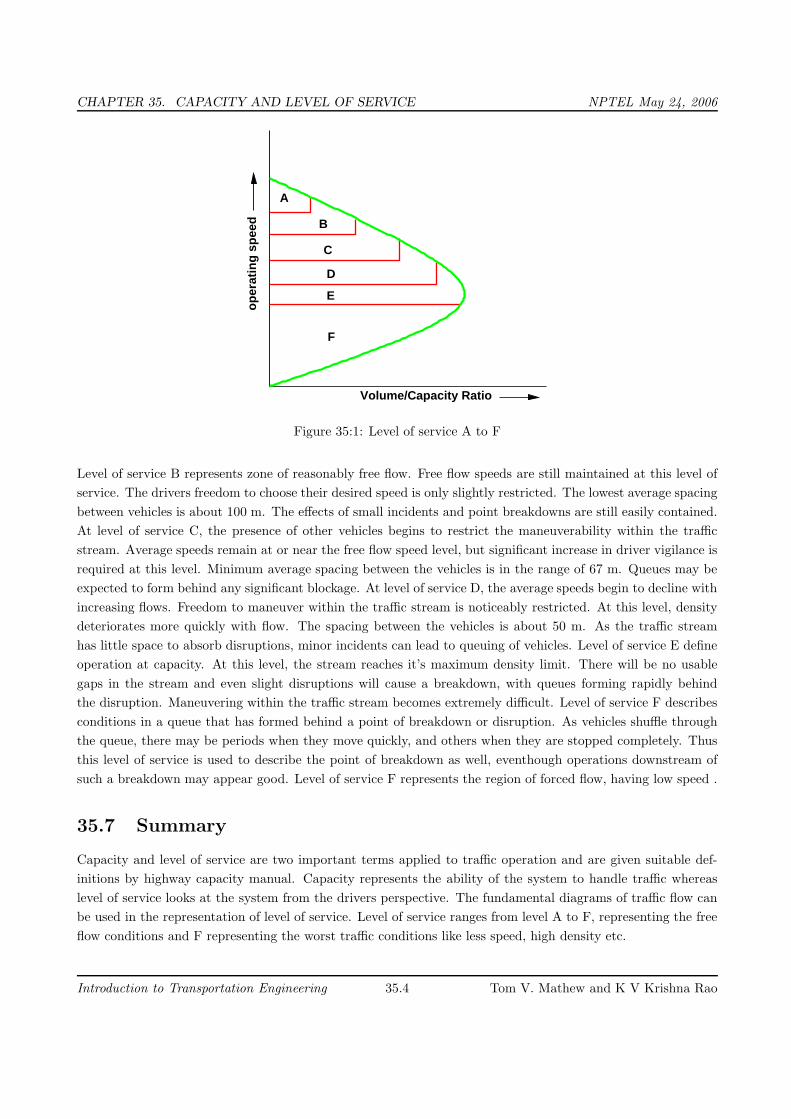
CHAPTER 35. CAPACITY AND LEVEL OF SERVICE NPTEL May 24, 2006
Volume/Capacity Ratio
op
erat
ing
sp
eed
A
C
B
D
F
E
Figure 35:1: Level of service A to F
Level of service B represents zone of reasonably free flow. Free flow speeds are still maintained at this level of
service. The drivers freedom to choose their desired speed is only slightly restricted. The lowest average spacing
between vehicles is about 100 m. The effects of small incidents and point breakdowns are still easily contained.
At level of service C, the presence of other vehicles begins to restrict the maneuverability within the traffic
stream. Average speeds remain at or near the free flow speed level, but significant increase in driver vigilance is
required at this level. Minimum average spacing between the vehicles is in the range of 67 m. Queues may be
expected to form behind any significant blockage. At level of service D, the average speeds begin to decline with
increasing flows. Freedom to maneuver within the traffic stream is noticeably restricted. At this level, density
deteriorates more quickly with flow. The spacing between the vehicles is about 50 m. As the traffic stream
has little space to absorb disruptions, minor incidents can lead to queuing of vehicles. Level of service E define
operation at capacity. At this level, the stream reaches it’s maximum density limit. There will be no usable
gaps in the stream and even slight disruptions will cause a breakdown, with queues forming rapidly behind
the disruption. Maneuvering within the traffic stream becomes extremely difficult. Level of service F describes
conditions in a queue that has formed behind a point of breakdown or disruption. As vehicles shuffle through
the queue, there may be periods when they move quickly, and others when they are stopped completely. Thus
this level of service is used to describe the point of breakdown as well, eventhough operations downstream of
such a breakdown may appear good. Level of service F represents the region of forced flow, having low speed .
35.7 Summary
Capacity and level of service are two important terms applied to traffic operation and are given suitable def-
initions by highway capacity manual. Capacity represents the ability of the system to handle traffic whereas
level of service looks at the system from the drivers perspective. The fundamental diagrams of traffic flow can
be used in the representation of level of service. Level of service ranges from level A to F, representing the free
flow conditions and F representing the worst traffic conditions like less speed, high density etc.
Introduction to Transportation Engineering 35.4 Tom V. Mathew and K V Krishna Rao
CHAPTER 35. CAPACITY AND LEVEL OF SERVICE NPTEL May 24, 2006
35.8 Problems
1. The parameter which is not used under measure of effectiveness
(a) Density
(b) Delay
(c) Speed
(d) Flow
2. How many levels of service are defined by HCM?
(a) Three
(b) Six
(c) Five
(d) Four
35.9 Solutions
1. The parameter which is not used under measure of effectiveness
(a) Density
(b) Delay
(c) Speed
(d) Flow√
2. How many levels of service are defined by HCM?
(a) Three
(b) Six√
(c) Five
(d) Four
Introduction to Transportation Engineering 35.5 Tom V. Mathew and K V Krishna Rao
CHAPTER 36. TRAFFIC SIGNS NPTEL May 24, 2006
Chapter 36
Traffic signs
36.1 Overview
Traffic control device is the medium used for communicating between traffic engineer and road users. Unlike
other modes of transportation, there is no control on the drivers using the road. Here traffic control devices
comes to the help of the traffic engineer. The major types of traffic control devices used are- traffic signs, road
markings , traffic signals and parking control. This chapter discusses traffic control signs. Different types of
traffic signs are regulatory signs, warning signs and informatory signs.
36.2 Requirements of traffic control devices
1. The control device should fulfill a need : Each device must have a specific purpose for the safe and
efficient operation of traffic flow. The superfluous devices should not be used.
2. It should command attention from the road users: This affects the design of signs. For commanding
attention, proper visibility should be there. Also the sign should be distinctive and clear. The sign should
be placed in such a way that the driver requires no extra effort to see the sign.
3. It should convey a clear, simple meaning: Clarity and simplicity of message is essential for the driver
to properly understand the meaning in short time. The use of color, shape and legend as codes becomes
important in this regard. The legend should be kept short and simple so that even a less educated driver
could understand the message in less time.
4. Road users must respect the signs: Respect is commanded only when the drivers are conditioned to
expect that all devices carry meaningful and important messages. Overuse, misuse and confusing messages
of devices tends the drivers to ignore them.
5. The control device should provide adequate time for proper response from the road users:
This is again related to the design aspect of traffic control devices. The sign boards should be placed at a
distance such that the driver could see it and gets sufficient time to respond to the situation. For example,
the STOP sign which is always placed at the stop line of the intersection should be visible for atleast one
safe stopping sight distance away from the stop line.
Introduction to Transportation Engineering 36.1 Tom V. Mathew and K V Krishna Rao
CHAPTER 36. TRAFFIC SIGNS NPTEL May 24, 2006
36.3 Communication tools
A number of mechanisms are used by the traffic engineer to communicate with the road user. These mecha-
nisms recognize certain human limitations, particularly eyesight. Messages are conveyed through the following
elements.
1. Color: It is the first and most easily noticed characteristics of a device. Usage of different colors for
different signs are important. The most commonly used colors are red, green, yellow, black, blue, and
brown . These are used to code certain devices and to reinforce specific messages. Consistent use of colors
helps the drivers to identify the presence of sign board ahead.
2. Shape : It is the second element discerned by the driver next to the color of the device. The categories of
shapes normally used are circular, triangular, rectangular, and diamond shape. Two exceptional shapes
used in traffic signs are octagonal shape for STOP sign and use of inverted triangle for GIVE WAY
(YIELD) sign. Diamond shape signs are not generally used in India.
3. Legend : This is the last element of a device that the drive comprehends. This is an important aspect
in the case of traffic signs. For the easy understanding by the driver, the legend should be short, simple
and specific so that it does not divert the attention of the driver. Symbols are normally used as legends
so that even a person unable to read the language will be able to understand that. There is no need of it
in the case of traffic signals and road markings.
4. Pattern: It is normally used in the application of road markings, complementing traffic signs. Generally
solid, double solid and dotted lines are used. Each pattern conveys different type of meaning. The frequent
and consistent use of pattern to convey information is recommended so that the drivers get accustomed
to the different types of markings and can instantly recognize them.
36.4 Types of traffic signs
There are several hundreds of traffic signs available covering wide variety of traffic situations. They can be
classified into three main categories.
1. Regulatory signs: These signs require the driver to obey the signs for the safety of other road users.
2. Warning signs:These signs are for the safety of oneself who is driving and advice the drivers to obey
these signs.
3. Informative signs: These signs provide information to the driver about the facilities available ahead,
and the route and distance to reach the specific destinations
In addition special type of traffic sign namely work zone signs are also available. These type of signs are used
to give warning to the road users when some construction work is going on the road. They are placed only for
short duration and will be removed soon after the work is over and when the road is brought back to its normal
condition. The first three signs will be discussed in detail below.
Introduction to Transportation Engineering 36.2 Tom V. Mathew and K V Krishna Rao
CHAPTER 36. TRAFFIC SIGNS NPTEL May 24, 2006
36.4.1 Regulatory signs
These signs are also called mandatory signs because it is mandatory that the drivers must obey these signs. If
the driver fails to obey them, the control agency has the right to take legal action against the driver. These
signs are primarily meant for the safety of other road users. These signs have generally black legend on a white
background. They are circular in shape with red borders. The regulatory signs can be further classified into :
1. Right of way series: These include two unique signs that assign the right of way to the selected
approaches of an intersection. They are the STOP sign and GIVE WAY sign For example, when one
minor road and major road meets at an intersection, preference should be given to the vehicles passing
through the major road. Hence the give way sign board will be placed on the minor road to inform the
driver on the minor road that he should give way for the vehicles on the major road. In case two major
roads are meeting, then the traffic engineer decides based on the traffic on which approach the sign board
has to be placed. Stop sign is another example of regulatory signs that comes in right of way series which
requires the driver to stop the vehicle at the stop line.
2. Speed series: Number of speed signs may be used to limit the speed of the vehicle on the road. They
include typical speed limit signs, truck speed, minimum speed signs etc. Speed limit signs are placed to
limit the speed of the vehicle to a particular speed for many reasons. Separate truck speed limits are
applied on high speed roadways where heavy commercial vehicles must be limited to slower speeds than
passenger cars for safety reasons. Minimum speed limits are applied on high speed roads like expressways,
freeways etc. where safety is again a predominant reason. Very slow vehicles may present hazard to
themselves and other vehicles also.
3. Movement series: They contain a number of signs that affect specific vehicle maneuvers. These include
turn signs, alignment signs, exclusion signs, one way signs etc. Turn signs include turn prohibitions and
lane use control signs. Lane use signs make use of arrows to specify the movements which all vehicles in
the lane must take. Turn signs are used to safely accommodate turns in unsignalized intersections.
4. Parking series: They include parking signs which indicate not only parking prohibitions or restrictions,
but also indicate places where parking is permitted, the type of vehicle to be parked, duration for parking
etc.
5. Pedestrian series: They include both legend and symbol signs. These signs are meant for the safety of
pedestrians and include signs indicating pedestrian only roads, pedestrian crossing sites etc.
6. Miscellaneous: Wide variety of signs that are included in this category are: a ”KEEP OF MEDIAN”
sign, signs indicating road closures, signs restricting vehicles carrying hazardous cargo or substances, signs
indicating vehicle weight limitations etc.
Some examples of the regulatory signs are shown in figure 36:1. They include a stop sign, give way sign, signs
for no entry, sign indicating prohibition for right turn, vehicle width limit sign, speed limit sign etc.
36.4.2 Warning signs
Warning signs or cautionary signs give information to the driver about the impending road condition. They
advice the driver to obey the rules. These signs are meant for the own safety of drivers. They call for extra
vigilance from the part of drivers. The color convention used for this type of signs is that the legend will be black
Introduction to Transportation Engineering 36.3 Tom V. Mathew and K V Krishna Rao
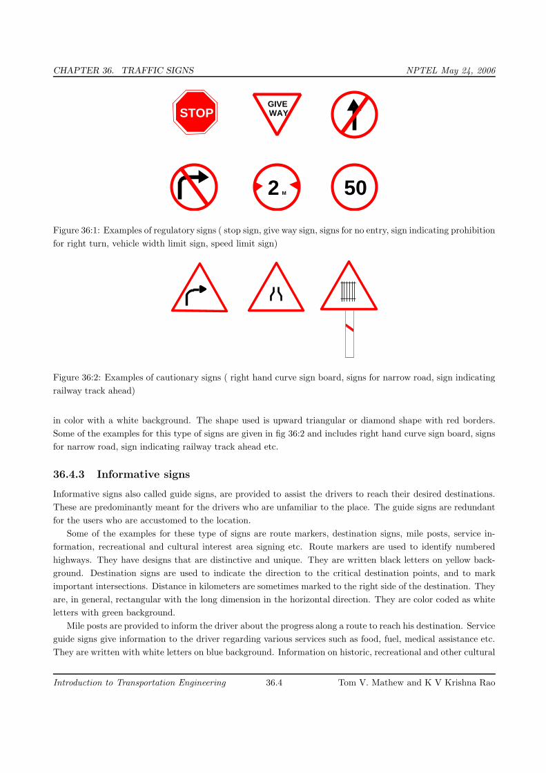
CHAPTER 36. TRAFFIC SIGNS NPTEL May 24, 2006
2 M
���� ��
�� 50
�������������������������������������������������������������������������������������������������������������������������������������������������������������������������������������������������������������������������������������������������������������������������������������������������������������������������������������������������������������������������
�������������������������������������������������������������������������������������������������������������������������������������������������������������������������������������������������������������������������������������������������������������������������������������������������������������������������������������������������������������������������
STOPGIVEWAY
Figure 36:1: Examples of regulatory signs ( stop sign, give way sign, signs for no entry, sign indicating prohibition
for right turn, vehicle width limit sign, speed limit sign)
������������������������������
Figure 36:2: Examples of cautionary signs ( right hand curve sign board, signs for narrow road, sign indicating
railway track ahead)
in color with a white background. The shape used is upward triangular or diamond shape with red borders.
Some of the examples for this type of signs are given in fig 36:2 and includes right hand curve sign board, signs
for narrow road, sign indicating railway track ahead etc.
36.4.3 Informative signs
Informative signs also called guide signs, are provided to assist the drivers to reach their desired destinations.
These are predominantly meant for the drivers who are unfamiliar to the place. The guide signs are redundant
for the users who are accustomed to the location.
Some of the examples for these type of signs are route markers, destination signs, mile posts, service in-
formation, recreational and cultural interest area signing etc. Route markers are used to identify numbered
highways. They have designs that are distinctive and unique. They are written black letters on yellow back-
ground. Destination signs are used to indicate the direction to the critical destination points, and to mark
important intersections. Distance in kilometers are sometimes marked to the right side of the destination. They
are, in general, rectangular with the long dimension in the horizontal direction. They are color coded as white
letters with green background.
Mile posts are provided to inform the driver about the progress along a route to reach his destination. Service
guide signs give information to the driver regarding various services such as food, fuel, medical assistance etc.
They are written with white letters on blue background. Information on historic, recreational and other cultural
Introduction to Transportation Engineering 36.4 Tom V. Mathew and K V Krishna Rao
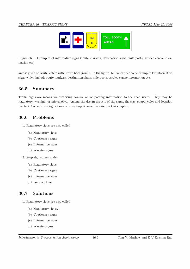
CHAPTER 36. TRAFFIC SIGNS NPTEL May 24, 2006
�������������������������������������������������������������������������������������������������������������������������������������������������������������������������������������������������������������������������������������������������������������������������������������������������������������������������������������������������������������������������������������������������������������������������������������������������������������������������������������������
�����������������������������������������������������������������������������������������������������������������������������������������������������������������������������������������������������������������������������������������������������������������������������������������������������������������������������������������������������������������������������������������������������������������������������������������
���������������������������������������������������������������������������������������������������������������������������������������������������������������������������������������������������������������������������������������������������������������
���������������������������������������������������������������������������������������������������������������������������������������������������������������������������������������������������������������������������������������������������������������
�������������������������
�������������������������
�������������������������
�������������������������
����������
����������
���������������
��������������������
� � � � � � � �
��������������������
�����������������������������������������������������������������������������������������������������������������������������������������������������������������������������������������������������������������������������������������������������������������������������������������������������������������������������������������������������������������������������������������������������������������������������������������
�����������������������������������������������������������������������������������������������������������������������������������������������������������������������������������������������������������������������������������������������������������������������������������������������������������������������������������������������������������������������������������������������������������������������������������������
�����������������������������������������������������������������������������������������������������������������������������������������������������������������������������������������������������������������������������
�����������������������������������������������������������������������������������������������������������������������������������������������������������������������������������������������������������������������������
TOLL BOOTH
AHEAD
����������������������������������������������������������������������������������������������������������������������������������������������������������������������������������������������������������������������������������������������������������������������������������������������������������������������������������������������������������������������������������������������������������������������������������������������������������
����������������������������������������������������������������������������������������������������������������������������������������������������������������������������������������������������������������������������������������������������������������������������������������������������������������������������������������������������������������������������������������������������������������������������������������������������������
NH �������
�������������������������������������������������
����������������������������������������
8
Figure 36:3: Examples of informative signs (route markers, destination signs, mile posts, service centre infor-
mation etc)
area is given on white letters with brown background. In the figure 36:3 we can see some examples for informative
signs which include route markers, destination signs, mile posts, service centre information etc..
36.5 Summary
Traffic signs are means for exercising control on or passing information to the road users. They may be
regulatory, warning, or informative. Among the design aspects of the signs, the size, shape, color and location
matters. Some of the signs along with examples were discussed in this chapter.
36.6 Problems
1. Regulatory signs are also called
(a) Mandatory signs
(b) Cautionary signs
(c) Informative signs
(d) Warning signs
2. Stop sign comes under
(a) Regulatory signs
(b) Cautionary signs
(c) Informative signs
(d) none of these
36.7 Solutions
1. Regulatory signs are also called
(a) Mandatory signs√
(b) Cautionary signs
(c) Informative signs
(d) Warning signs
Introduction to Transportation Engineering 36.5 Tom V. Mathew and K V Krishna Rao
CHAPTER 36. TRAFFIC SIGNS NPTEL May 24, 2006
2. Stop sign comes under
(a) Regulatory signs√
(b) Cautionary signs
(c) Informative signs
(d) none of these
Introduction to Transportation Engineering 36.6 Tom V. Mathew and K V Krishna Rao
CHAPTER 37. ROAD MARKINGS NPTEL May 24, 2006
Chapter 37
Road markings
37.1 Overview
The essential purpose of road markings is to guide and control traffic on a highway. They supplement the
function of traffic signs. The markings serve as a psychological barrier and signify the delineation of traffic path
and its lateral clearance from traffic hazards for the safe movement of traffic. Hence they are very important
to ensure the safe, smooth and harmonious flow of traffic. Various types of road markings like longitudinal
markings, transverse markings, object markings and special markings to warn the driver about the hazardous
locations in the road etc. will be discussed in detail in this chapter.
37.2 Classification of road markings
The road markings are defined as lines, patterns, words or other devices, except signs, set into applied or attached
to the carriageway or kerbs or to objects within or adjacent to the carriageway, for controlling, warning, guiding
and informing the users. The road markings are classified as longitudinal markings, transverse markings, object
markings, word messages, marking for parkings, marking at hazardous locations etc.
37.3 Longitudinal markings
Longitudinal markings are placed along the direction of traffic on the roadway surface, for the purpose of
indicating to the driver, his proper position on the roadway. Some of the guiding principles in longitudinal
markings are also discussed below.
Longitudinal markings are provided for separating traffic flow in the same direction and the predominant
color used is white. Yellow color is used to separate the traffic flow in opposite direction and also to separate the
pavement edges. The lines can be either broken, solid or double solid. Broken lines are permissive in character
and allows crossing with discretion, if traffic situation permits. Solid lines are restrictive in character and does
not allow crossing except for entry or exit from a side road or premises or to avoid a stationary obstruction.
Double solid lines indicate severity in restrictions and should not be crossed except in case of emergency. There
can also be a combination of solid and broken lines. In such a case, a solid line may be crossed with discretion,
if the broken line of the combination is nearer to the direction of travel. Vehicles from the opposite directions
are not permitted to cross the line. Different types of longitudinal markings are centre line, traffic lanes, no
passing zone, warning lines, border or edge lines, bus lane markings, cycle lane markings.
Introduction to Transportation Engineering 37.1 Tom V. Mathew and K V Krishna Rao
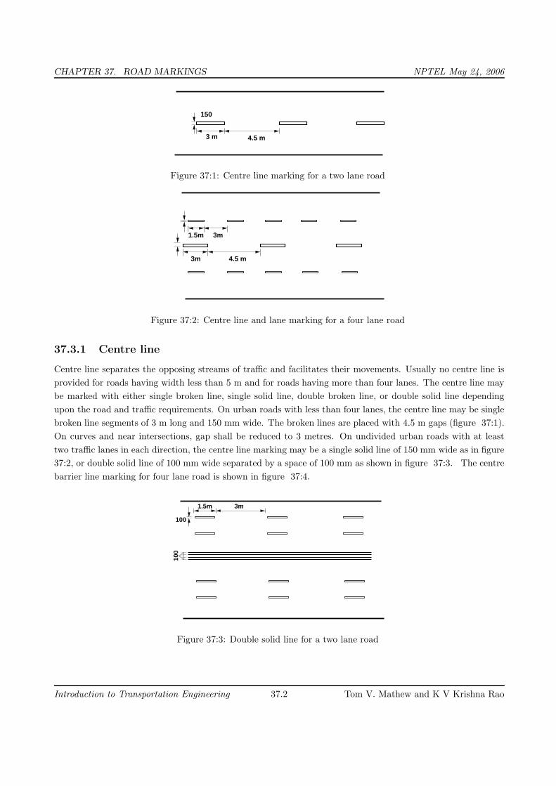
CHAPTER 37. ROAD MARKINGS NPTEL May 24, 2006
150
4.5 m3 m
Figure 37:1: Centre line marking for a two lane road
1.5m 3m
3m 4.5 m
Figure 37:2: Centre line and lane marking for a four lane road
37.3.1 Centre line
Centre line separates the opposing streams of traffic and facilitates their movements. Usually no centre line is
provided for roads having width less than 5 m and for roads having more than four lanes. The centre line may
be marked with either single broken line, single solid line, double broken line, or double solid line depending
upon the road and traffic requirements. On urban roads with less than four lanes, the centre line may be single
broken line segments of 3 m long and 150 mm wide. The broken lines are placed with 4.5 m gaps (figure 37:1).
On curves and near intersections, gap shall be reduced to 3 metres. On undivided urban roads with at least
two traffic lanes in each direction, the centre line marking may be a single solid line of 150 mm wide as in figure
37:2, or double solid line of 100 mm wide separated by a space of 100 mm as shown in figure 37:3. The centre
barrier line marking for four lane road is shown in figure 37:4.
100
100
1.5m 3m
Figure 37:3: Double solid line for a two lane road
Introduction to Transportation Engineering 37.2 Tom V. Mathew and K V Krishna Rao
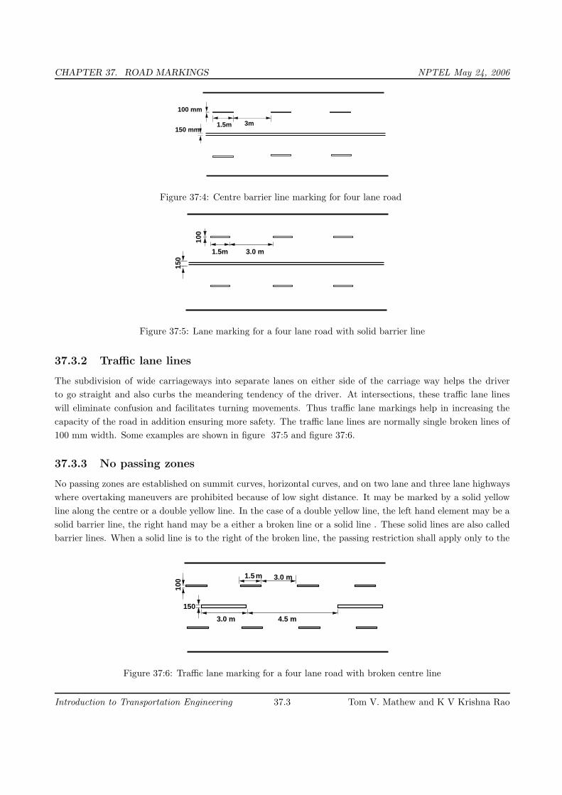
CHAPTER 37. ROAD MARKINGS NPTEL May 24, 2006
150 mm
100 mm
3m1.5m
Figure 37:4: Centre barrier line marking for four lane road
3.0 m
100
150
1.5m
Figure 37:5: Lane marking for a four lane road with solid barrier line
37.3.2 Traffic lane lines
The subdivision of wide carriageways into separate lanes on either side of the carriage way helps the driver
to go straight and also curbs the meandering tendency of the driver. At intersections, these traffic lane lines
will eliminate confusion and facilitates turning movements. Thus traffic lane markings help in increasing the
capacity of the road in addition ensuring more safety. The traffic lane lines are normally single broken lines of
100 mm width. Some examples are shown in figure 37:5 and figure 37:6.
37.3.3 No passing zones
No passing zones are established on summit curves, horizontal curves, and on two lane and three lane highways
where overtaking maneuvers are prohibited because of low sight distance. It may be marked by a solid yellow
line along the centre or a double yellow line. In the case of a double yellow line, the left hand element may be a
solid barrier line, the right hand may be a either a broken line or a solid line . These solid lines are also called
barrier lines. When a solid line is to the right of the broken line, the passing restriction shall apply only to the
100
150
1.5 m 3.0 m
3.0 m 4.5 m
Figure 37:6: Traffic lane marking for a four lane road with broken centre line
Introduction to Transportation Engineering 37.3 Tom V. Mathew and K V Krishna Rao
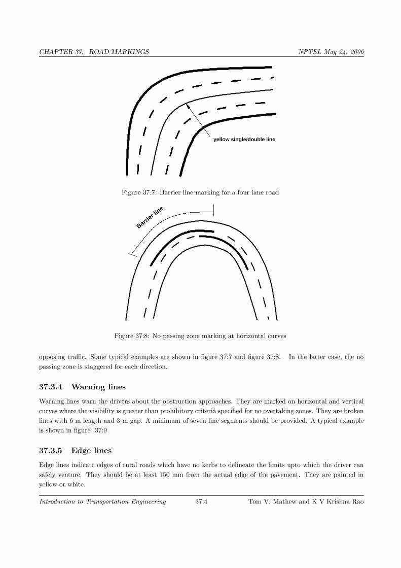
CHAPTER 37. ROAD MARKINGS NPTEL May 24, 2006
yellow single/double line
Figure 37:7: Barrier line marking for a four lane road
Barrier li
ne
Figure 37:8: No passing zone marking at horizontal curves
opposing traffic. Some typical examples are shown in figure 37:7 and figure 37:8. In the latter case, the no
passing zone is staggered for each direction.
37.3.4 Warning lines
Warning lines warn the drivers about the obstruction approaches. They are marked on horizontal and vertical
curves where the visibility is greater than prohibitory criteria specified for no overtaking zones. They are broken
lines with 6 m length and 3 m gap. A minimum of seven line segments should be provided. A typical example
is shown in figure 37:9
37.3.5 Edge lines
Edge lines indicate edges of rural roads which have no kerbs to delineate the limits upto which the driver can
safely venture. They should be at least 150 mm from the actual edge of the pavement. They are painted in
yellow or white.
Introduction to Transportation Engineering 37.4 Tom V. Mathew and K V Krishna Rao
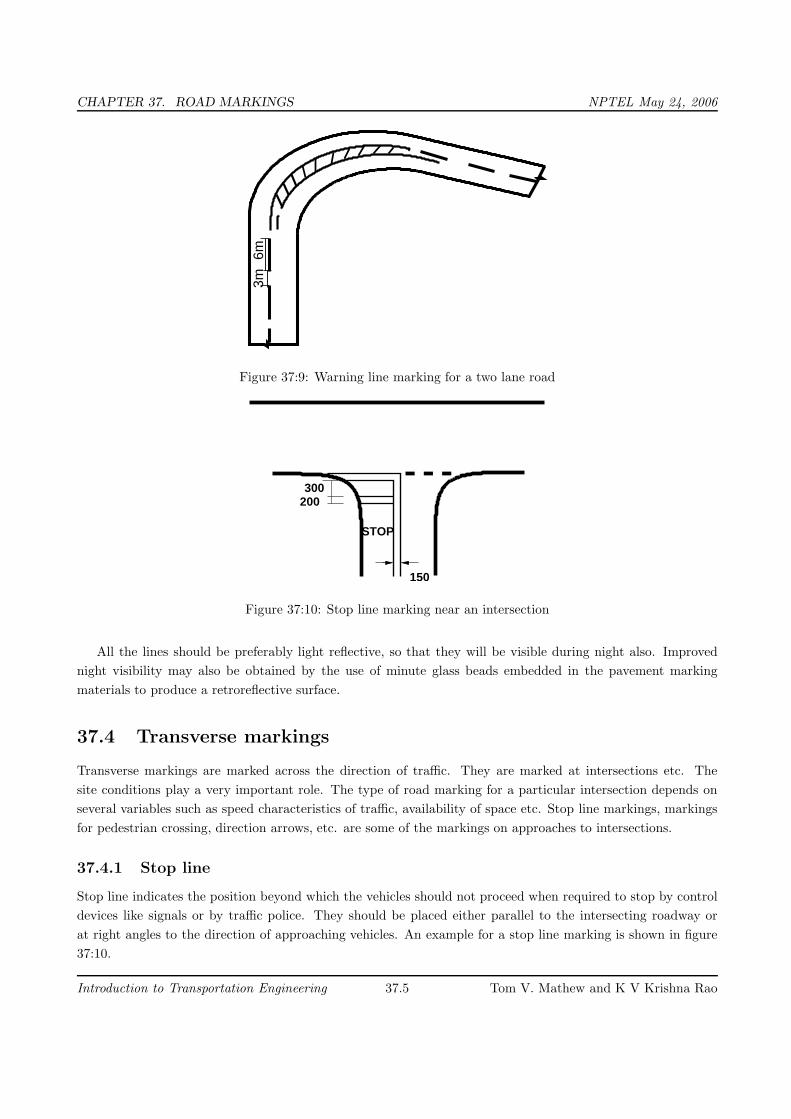
CHAPTER 37. ROAD MARKINGS NPTEL May 24, 2006
3m6m
Figure 37:9: Warning line marking for a two lane road
300200
STOP
150
Figure 37:10: Stop line marking near an intersection
All the lines should be preferably light reflective, so that they will be visible during night also. Improved
night visibility may also be obtained by the use of minute glass beads embedded in the pavement marking
materials to produce a retroreflective surface.
37.4 Transverse markings
Transverse markings are marked across the direction of traffic. They are marked at intersections etc. The
site conditions play a very important role. The type of road marking for a particular intersection depends on
several variables such as speed characteristics of traffic, availability of space etc. Stop line markings, markings
for pedestrian crossing, direction arrows, etc. are some of the markings on approaches to intersections.
37.4.1 Stop line
Stop line indicates the position beyond which the vehicles should not proceed when required to stop by control
devices like signals or by traffic police. They should be placed either parallel to the intersecting roadway or
at right angles to the direction of approaching vehicles. An example for a stop line marking is shown in figure
37:10.
Introduction to Transportation Engineering 37.5 Tom V. Mathew and K V Krishna Rao
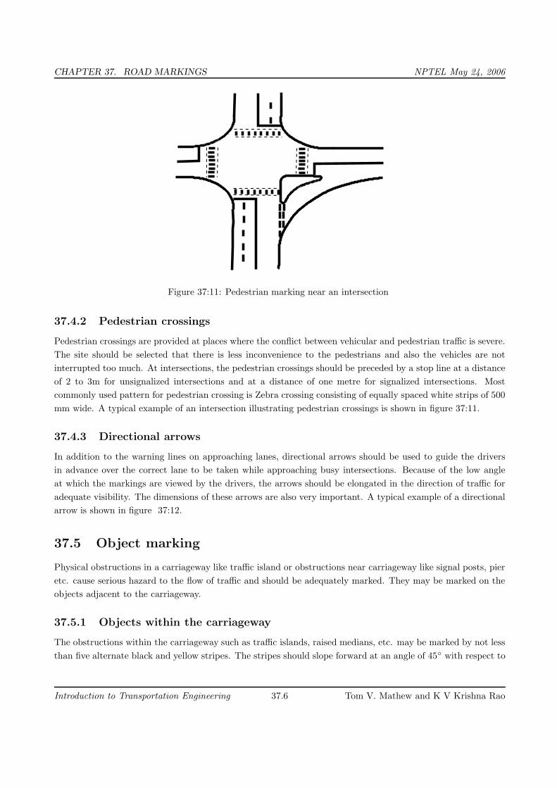
CHAPTER 37. ROAD MARKINGS NPTEL May 24, 2006
Figure 37:11: Pedestrian marking near an intersection
37.4.2 Pedestrian crossings
Pedestrian crossings are provided at places where the conflict between vehicular and pedestrian traffic is severe.
The site should be selected that there is less inconvenience to the pedestrians and also the vehicles are not
interrupted too much. At intersections, the pedestrian crossings should be preceded by a stop line at a distance
of 2 to 3m for unsignalized intersections and at a distance of one metre for signalized intersections. Most
commonly used pattern for pedestrian crossing is Zebra crossing consisting of equally spaced white strips of 500
mm wide. A typical example of an intersection illustrating pedestrian crossings is shown in figure 37:11.
37.4.3 Directional arrows
In addition to the warning lines on approaching lanes, directional arrows should be used to guide the drivers
in advance over the correct lane to be taken while approaching busy intersections. Because of the low angle
at which the markings are viewed by the drivers, the arrows should be elongated in the direction of traffic for
adequate visibility. The dimensions of these arrows are also very important. A typical example of a directional
arrow is shown in figure 37:12.
37.5 Object marking
Physical obstructions in a carriageway like traffic island or obstructions near carriageway like signal posts, pier
etc. cause serious hazard to the flow of traffic and should be adequately marked. They may be marked on the
objects adjacent to the carriageway.
37.5.1 Objects within the carriageway
The obstructions within the carriageway such as traffic islands, raised medians, etc. may be marked by not less
than five alternate black and yellow stripes. The stripes should slope forward at an angle of 45◦ with respect to
Introduction to Transportation Engineering 37.6 Tom V. Mathew and K V Krishna Rao
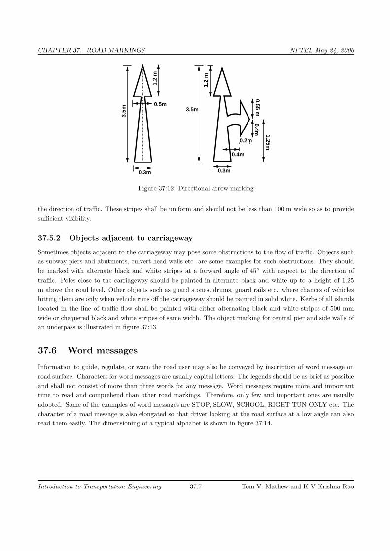
CHAPTER 37. ROAD MARKINGS NPTEL May 24, 2006
0.3m0.3m
3.5m
0.2m
1.25m
0.4m0.55 m
0.4m
1.2
m
0.5m
3.5m
1.2
m
Figure 37:12: Directional arrow marking
the direction of traffic. These stripes shall be uniform and should not be less than 100 m wide so as to provide
sufficient visibility.
37.5.2 Objects adjacent to carriageway
Sometimes objects adjacent to the carriageway may pose some obstructions to the flow of traffic. Objects such
as subway piers and abutments, culvert head walls etc. are some examples for such obstructions. They should
be marked with alternate black and white stripes at a forward angle of 45◦ with respect to the direction of
traffic. Poles close to the carriageway should be painted in alternate black and white up to a height of 1.25
m above the road level. Other objects such as guard stones, drums, guard rails etc. where chances of vehicles
hitting them are only when vehicle runs off the carriageway should be painted in solid white. Kerbs of all islands
located in the line of traffic flow shall be painted with either alternating black and white stripes of 500 mm
wide or chequered black and white stripes of same width. The object marking for central pier and side walls of
an underpass is illustrated in figure 37:13.
37.6 Word messages
Information to guide, regulate, or warn the road user may also be conveyed by inscription of word message on
road surface. Characters for word messages are usually capital letters. The legends should be as brief as possible
and shall not consist of more than three words for any message. Word messages require more and important
time to read and comprehend than other road markings. Therefore, only few and important ones are usually
adopted. Some of the examples of word messages are STOP, SLOW, SCHOOL, RIGHT TUN ONLY etc. The
character of a road message is also elongated so that driver looking at the road surface at a low angle can also
read them easily. The dimensioning of a typical alphabet is shown in figure 37:14.
Introduction to Transportation Engineering 37.7 Tom V. Mathew and K V Krishna Rao
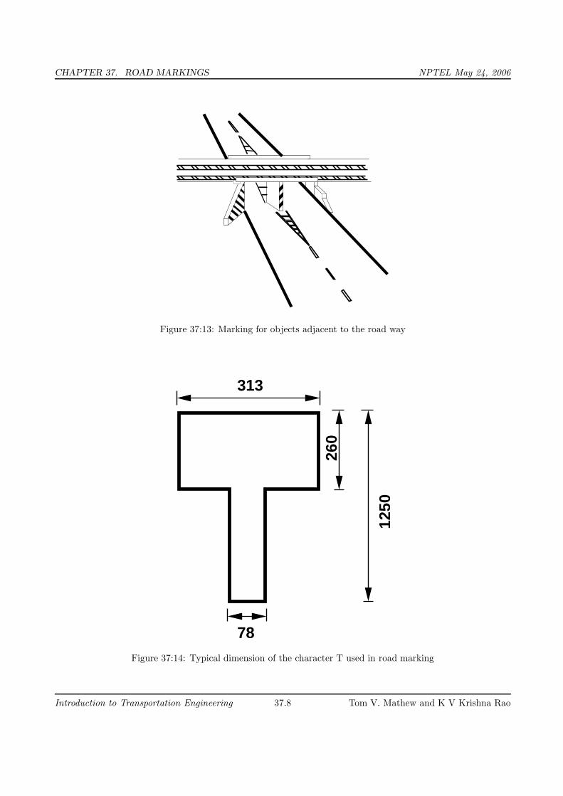
CHAPTER 37. ROAD MARKINGS NPTEL May 24, 2006
Figure 37:13: Marking for objects adjacent to the road way
313
78
260
1250
Figure 37:14: Typical dimension of the character T used in road marking
Introduction to Transportation Engineering 37.8 Tom V. Mathew and K V Krishna Rao
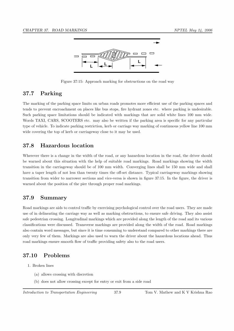
CHAPTER 37. ROAD MARKINGS NPTEL May 24, 2006
LLL
Figure 37:15: Approach marking for obstructions on the road way
37.7 Parking
The marking of the parking space limits on urban roads promotes more efficient use of the parking spaces and
tends to prevent encroachment on places like bus stops, fire hydrant zones etc. where parking is undesirable.
Such parking space limitations should be indicated with markings that are solid white lines 100 mm wide.
Words TAXI, CARS, SCOOTERS etc. may also be written if the parking area is specific for any particular
type of vehicle. To indicate parking restriction, kerb or carriage way marking of continuous yellow line 100 mm
wide covering the top of kerb or carriageway close to it may be used.
37.8 Hazardous location
Wherever there is a change in the width of the road, or any hazardous location in the road, the driver should
be warned about this situation with the help of suitable road markings. Road markings showing the width
transition in the carriageway should be of 100 mm width. Converging lines shall be 150 mm wide and shall
have a taper length of not less than twenty times the off-set distance. Typical carriageway markings showing
transition from wider to narrower sections and vice-versa is shown in figure 37:15. In the figure, the driver is
warned about the position of the pier through proper road markings.
37.9 Summary
Road markings are aids to control traffic by exercising psychological control over the road users. They are made
use of in delineating the carriage way as well as marking obstructions, to ensure safe driving. They also assist
safe pedestrian crossing. Longitudinal markings which are provided along the length of the road and its various
classifications were discussed. Transverse markings are provided along the width of the road. Road markings
also contain word messages, but since it is time consuming to understand compared to other markings there are
only very few of them. Markings are also used to warn the driver about the hazardous locations ahead. Thus
road markings ensure smooth flow of traffic providing safety also to the road users.
37.10 Problems
1. Broken lines
(a) allows crossing with discretion
(b) does not allow crossing except for entry or exit from a side road
Introduction to Transportation Engineering 37.9 Tom V. Mathew and K V Krishna Rao
CHAPTER 37. ROAD MARKINGS NPTEL May 24, 2006
(c) allows crossing only in case of extreme emergency
(d) are not at all used as road markings.
2. Stop line comes under
(a) Longitudinal markings
(b) Object markings
(c) Transverse markings
(d) None of these
37.11 Solutions
1. Broken lines
(a) allows crossing with discretion√
(b) does not allow crossing except for entry or exit from a side road
(c) allows crossing only in case of extreme emergency
(d) are not at all used as road markings.
2. Stop line comes under
(a) Longitudinal markings
(b) Object markings
(c) Transverse markings√
(d) None of these
Introduction to Transportation Engineering 37.10 Tom V. Mathew and K V Krishna Rao
CHAPTER 38. PARKING NPTEL May 24, 2006
Chapter 38
Parking
38.1 Overview
Parking is one of the major problems that is created by the increasing road traffic. It is an impact of transport
development. The availability of less space in urban areas has increased the demand for parking space especially
in areas like Central business district. This affects the mode choice also. This has a great economical impact.
38.2 Parking studies
Before taking any measures for the betterment of conditions, data regarding availability of parking space, extent
of its usage and parking demand is essential. It is also required to estimate the parking fares also. Parking
surveys are intended to provide all these information. Since the duration of parking varies with different vehicles,
several statistics are used to access the parking need.
38.2.1 Parking statistics
Parking accumulation: It is defined as the number of vehicles parked at a given instant of time.
Normally this is expressed by accumulation curve. Accumulation curve is the graph obtained by plotting
the number of bays occupied with respect to time.
Parking volume: Parking volume is the total number of vehicles parked at a given duration of time.
This does not account for repetition of vehicles.
Parking load : Parking load gives the area under the accumulation curve. It can also be obtained by
simply multiplying the number of vehicles occupying the parking area at each time interval with the time
interval. It is expressed as vehicle hours.
Average parking duration: It is the ratio of total vehicle hours to the number of vehicles parked.
Parking turnover: It is the ratio of number of vehicles parked in a duration to the number of parking
bays available. This can be expressed as number of vehicles per bay per time duration.
Parking index: Parking index is also called occupancy or efficiency. It is defined as the ratio of number
of bays occupied in a time duration to the total space available. It gives an aggregate measure of how
effectively the parking space is utilized. Parking index can be found out as follows
parking index =parking load
parking capacity× 100 (38.1)
Introduction to Transportation Engineering 38.1 Tom V. Mathew and K V Krishna Rao
CHAPTER 38. PARKING NPTEL May 24, 2006
38.3 Parking surveys
Parking surveys are conducted to collect the above said parking statistics. The most common parking surveys
conducted are in-out survey, fixed period sampling and license plate method of survey.
1. In-out survey: In this survey, the occupancy count in the selected parking lot is taken at the beginning.
Then the number of vehicles that enter the parking lot for a particular time interval is counted. The
number of vehicles that leave the parking lot is also taken. The final occupancy in the parking lot is also
taken. Here the labor required is very less. Only one person may be enough. But we wont get any data
regarding the time duration for which a particular vehicle used that parking lot. Parking duration and
turn over is not obtained. Hence we cannot estimate the parking fare from this survey.
2. Fixed period sampling: This is almost similar to in-out survey. All vehicles are counted at the
beginning of the survey. Then after a fixed time interval that may vary between 15 minutes to i hour,
the count is again taken. Here there are chances of missing the number of vehicles that were parked for a
short duration.
3. License plate method of survey: This results in the most accurate and realistic data. In this case
of survey, every parking stall is monitored at a continuous interval of 15 minutes or so and the license
plate number is noted down. This will give the data regarding the duration for which a particular vehicle
was using the parking bay. This will help in calculating the fare because fare is estimated based on the
duration for which the vehicle was parked. If the time interval is shorter, then there are less chances of
missing short-term parkers. But this method is very labor intensive.
38.4 Ill effects of parking
Parking has some ill-effects like congestion, accidents, pollution, obstruction to fire-fighting operations etc.
Congestion: Parking takes considerable street space leading to the lowering of the road capacity. Hence,
speed will be reduced, journey time and delay will also subsequently increase. The operational cost of the
vehicle increases leading to great economical loss to the community.
Accidents: Careless maneuvering of parking and unparking leads to accidents which are referred to as
parking accidents. Common type of parking accidents occur while driving out a car from the parking
area, careless opening of the doors of parked cars, and while bringing in the vehicle to the parking lot for
parking.
Environmental pollution: They also cause pollution to the environment because stopping and starting
of vehicles while parking and unparking results in noise and fumes. They also affect the aesthetic beauty
of the buildings because cars parked at every available space creates a feeling that building rises from a
plinth of cars.
Obstruction to fire fighting operations: Parked vehicles may obstruct the movement of firefighting
vehicles. Sometimes they block access to hydrants and access to buildings.
Introduction to Transportation Engineering 38.2 Tom V. Mathew and K V Krishna Rao
CHAPTER 38. PARKING NPTEL May 24, 2006
L
2.5
5.0
5.9
Figure 38:1: Illustration of parallel parking
38.5 Parking requirements
There are some minimum parking requirements for different types of building. For residential plot area less
than 300 sq.m require only community parking space. For residential plot area from 500 to 1000 sq.m, minimum
one-fourth of the open area should be reserved for parking. Offices may require atleast one space for every 70
sq.m as parking area. One parking space is enough for 10 seats in a restaurant where as theatres and cinema
halls need to keep only 1 parking space for 20 seats. Thus, the parking requirements are different for different
land use zones.
38.6 On street parking
On street parking means the vehicles are parked on the sides of the street itself. This will be usually controlled
by government agencies itself. Common types of on-street parking are as listed below. This classification is
based on the angle in which the vehicles are parked with respect to the road alignment. As per IRC the standard
dimensions of a car is taken as 5× 2.5 metres and that for a truck is 3.75× 7.5 metres.
Parallel parking: The vehicles are parked along the length of the road. Here there is no backward
movement involved while parking or unparking the vehicle. Hence, it is the most safest parking from
the accident perspective. However, it consumes the maximum curb length and therefore only a minimum
number of vehicles can be parked for a given kerb length. This method of parking produces least obstruc-
tion to the on-going traffic on the road since least road width is used. Parallel parking of cars is shown in
figure 38:1. The length available to park N number of vehicles, L = N
5.9
30◦ parking: In thirty degree parking, the vehicles are parked at 30◦ with respect to the road alignment.
In this case, more vehicles can be parked compared to parallel parking. Also there is better maneuver-
ability. Delay caused to the traffic is also minimum in this type of parking. An example is shown in
figure 38:2. From the figure,
AB = OBsin30◦ = 1.25, BC = OPcos30◦ = 4.33, BD = DQcos60◦ = 5, CD = BD − BC = 5 − 4.33 = 0.67, AB + BC = 1.25 + 4.33 = 5.58
For N vehicles, L = AC + (N-1)CE =5.58+(N-1)5 =0.58+5N
45◦ parking: As the angle of parking increases, more number of vehicles can be parked. Hence compared
to parallel parking and thirty degree parking, more number of vehicles can be accommodated in this type
of parking. From figure 38:3, length of parking space available for parking N number of vehicles in a given
kerb is L = 3.54 N+1.77
Introduction to Transportation Engineering 38.3 Tom V. Mathew and K V Krishna Rao
CHAPTER 38. PARKING NPTEL May 24, 2006
5 m
2.5
m
30
1.25 m
4.66 m1 2 n....
A B C D E
L1.254.33
O QP
Figure 38:2: Illustration of 30◦ parking
5.0 m
45
1.77
5.31 m
2.5 m
Figure 38:3: Illustration of 45◦ parking
60◦ parking: The vehicles are parked at 60◦ to the direction of road. More number of vehicles can
be accommodated in this parking type. From the figure 38:4, length available for parking N vehicles
=2.89N+2.16.
Right angle parking: In right angle parking or 90◦ parking, the vehicles are parked perpendicular to
the direction of the road. Although it consumes maximum width kerb length required is very little. In
this type of parking, the vehicles need complex maneuvering and this may cause severe accidents. This
arrangement causes obstruction to the road traffic particularly if the road width is less. However, it can
accommodate maximum number of vehicles for a given kerb length. An example is shown in figure 38:5.
Length available for parking N number of vehicles is L = 2.5N.
2.5
L
60
Figure 38:4: Illustration of 60◦ parking
Introduction to Transportation Engineering 38.4 Tom V. Mathew and K V Krishna Rao
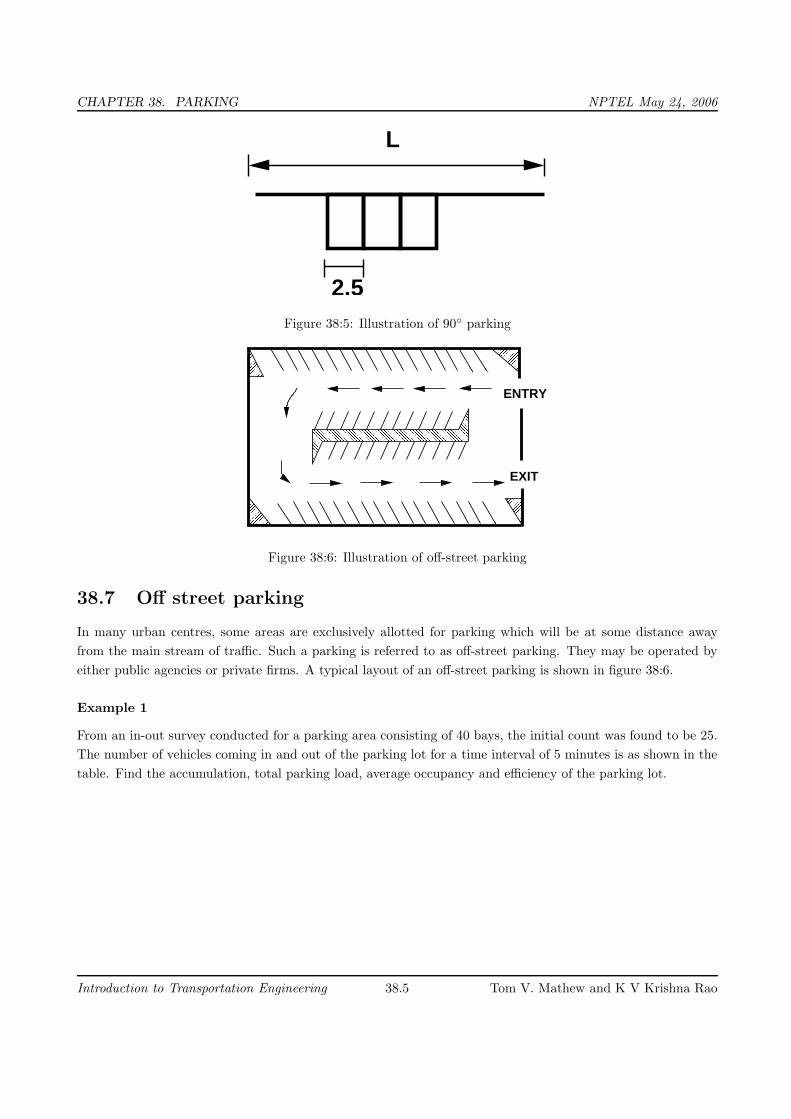
CHAPTER 38. PARKING NPTEL May 24, 2006
L
2.5Figure 38:5: Illustration of 90◦ parking
�������������������������
�������������������������
�����������������������������������
�����������������������������������
��������������������������������������������
��������������������������������������������
�����������������������������������
�������������������������
���������������������������������������������������������������������������������������������������������������������������������������������������������������������������������������������������������������������������������
������������������������������������������������������������������������������������������������������������������������������������������������������������������������������������������������������������������������
����������������������������
����������������������������
� � � � � � � � � � � �
��������������������
�����������������������������������
�����������������������������������
�����������������������������������
�����������������������������������
ENTRY
EXIT
Figure 38:6: Illustration of off-street parking
38.7 Off street parking
In many urban centres, some areas are exclusively allotted for parking which will be at some distance away
from the main stream of traffic. Such a parking is referred to as off-street parking. They may be operated by
either public agencies or private firms. A typical layout of an off-street parking is shown in figure 38:6.
Example 1
From an in-out survey conducted for a parking area consisting of 40 bays, the initial count was found to be 25.
The number of vehicles coming in and out of the parking lot for a time interval of 5 minutes is as shown in the
table. Find the accumulation, total parking load, average occupancy and efficiency of the parking lot.
Introduction to Transportation Engineering 38.5 Tom V. Mathew and K V Krishna Rao
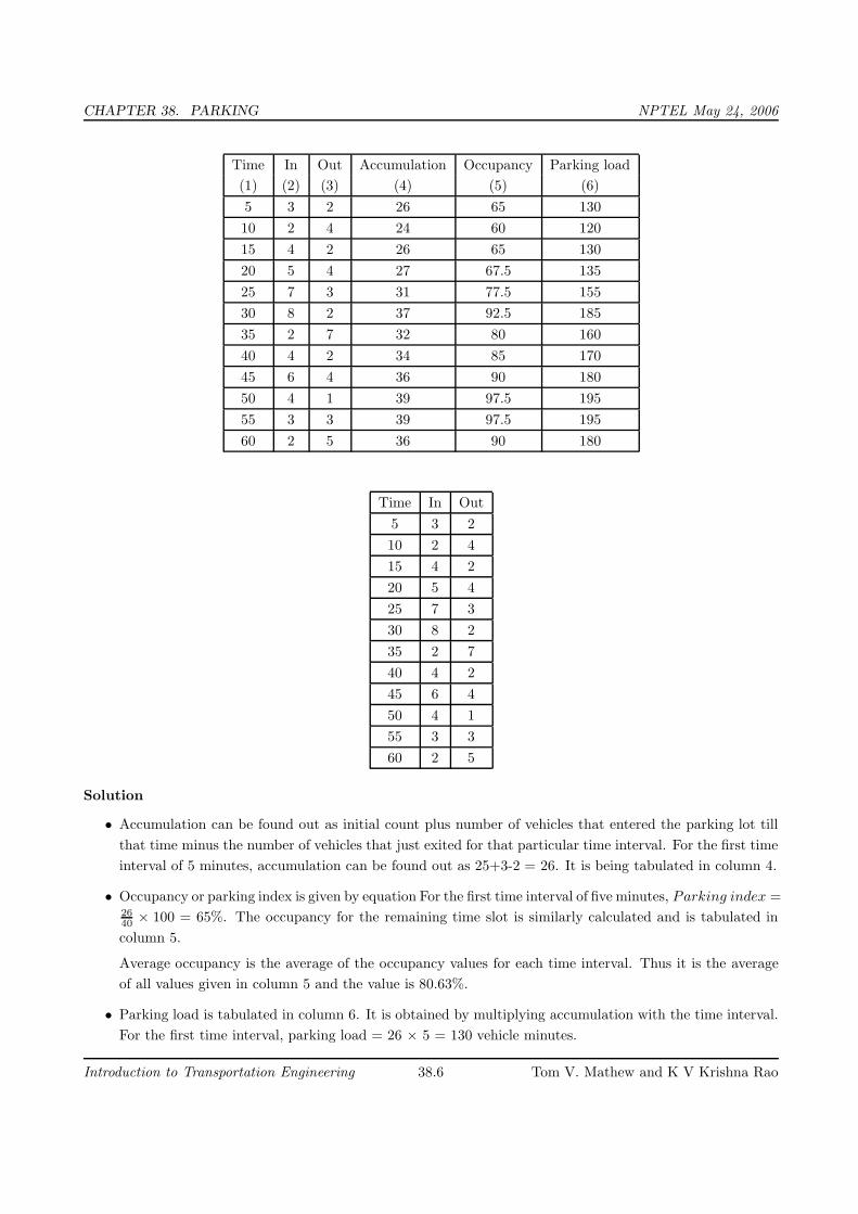
CHAPTER 38. PARKING NPTEL May 24, 2006
Time In Out Accumulation Occupancy Parking load
(1) (2) (3) (4) (5) (6)
5 3 2 26 65 130
10 2 4 24 60 120
15 4 2 26 65 130
20 5 4 27 67.5 135
25 7 3 31 77.5 155
30 8 2 37 92.5 185
35 2 7 32 80 160
40 4 2 34 85 170
45 6 4 36 90 180
50 4 1 39 97.5 195
55 3 3 39 97.5 195
60 2 5 36 90 180
Time In Out
5 3 2
10 2 4
15 4 2
20 5 4
25 7 3
30 8 2
35 2 7
40 4 2
45 6 4
50 4 1
55 3 3
60 2 5
Solution
• Accumulation can be found out as initial count plus number of vehicles that entered the parking lot till
that time minus the number of vehicles that just exited for that particular time interval. For the first time
interval of 5 minutes, accumulation can be found out as 25+3-2 = 26. It is being tabulated in column 4.
• Occupancy or parking index is given by equation For the first time interval of five minutes, Parking index =26
40× 100 = 65%. The occupancy for the remaining time slot is similarly calculated and is tabulated in
column 5.
Average occupancy is the average of the occupancy values for each time interval. Thus it is the average
of all values given in column 5 and the value is 80.63%.
• Parking load is tabulated in column 6. It is obtained by multiplying accumulation with the time interval.
For the first time interval, parking load = 26 × 5 = 130 vehicle minutes.
Introduction to Transportation Engineering 38.6 Tom V. Mathew and K V Krishna Rao
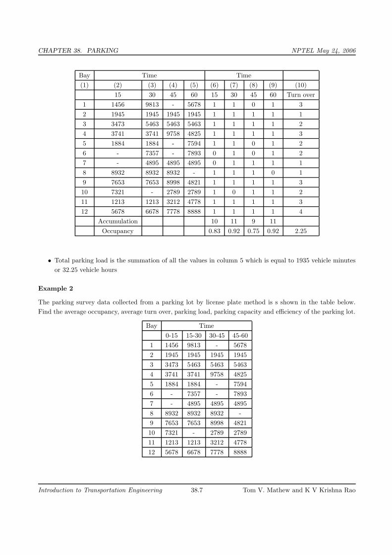
CHAPTER 38. PARKING NPTEL May 24, 2006
Bay Time Time
(1) (2) (3) (4) (5) (6) (7) (8) (9) (10)
15 30 45 60 15 30 45 60 Turn over
1 1456 9813 - 5678 1 1 0 1 3
2 1945 1945 1945 1945 1 1 1 1 1
3 3473 5463 5463 5463 1 1 1 1 2
4 3741 3741 9758 4825 1 1 1 1 3
5 1884 1884 - 7594 1 1 0 1 2
6 - 7357 - 7893 0 1 0 1 2
7 - 4895 4895 4895 0 1 1 1 1
8 8932 8932 8932 - 1 1 1 0 1
9 7653 7653 8998 4821 1 1 1 1 3
10 7321 - 2789 2789 1 0 1 1 2
11 1213 1213 3212 4778 1 1 1 1 3
12 5678 6678 7778 8888 1 1 1 1 4
Accumulation 10 11 9 11
Occupancy 0.83 0.92 0.75 0.92 2.25
• Total parking load is the summation of all the values in column 5 which is equal to 1935 vehicle minutes
or 32.25 vehicle hours
Example 2
The parking survey data collected from a parking lot by license plate method is s shown in the table below.
Find the average occupancy, average turn over, parking load, parking capacity and efficiency of the parking lot.
Bay Time
0-15 15-30 30-45 45-60
1 1456 9813 - 5678
2 1945 1945 1945 1945
3 3473 5463 5463 5463
4 3741 3741 9758 4825
5 1884 1884 - 7594
6 - 7357 - 7893
7 - 4895 4895 4895
8 8932 8932 8932 -
9 7653 7653 8998 4821
10 7321 - 2789 2789
11 1213 1213 3212 4778
12 5678 6678 7778 8888
Introduction to Transportation Engineering 38.7 Tom V. Mathew and K V Krishna Rao
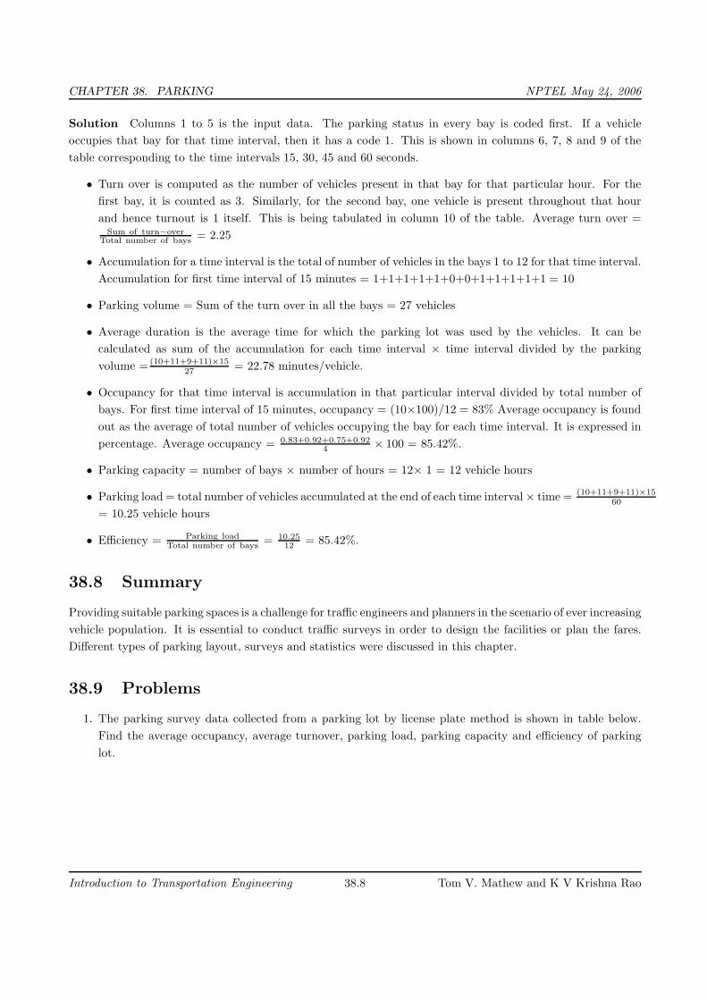
CHAPTER 38. PARKING NPTEL May 24, 2006
Solution Columns 1 to 5 is the input data. The parking status in every bay is coded first. If a vehicle
occupies that bay for that time interval, then it has a code 1. This is shown in columns 6, 7, 8 and 9 of the
table corresponding to the time intervals 15, 30, 45 and 60 seconds.
• Turn over is computed as the number of vehicles present in that bay for that particular hour. For the
first bay, it is counted as 3. Similarly, for the second bay, one vehicle is present throughout that hour
and hence turnout is 1 itself. This is being tabulated in column 10 of the table. Average turn over =Sum of turn−over
Total number of bays= 2.25
• Accumulation for a time interval is the total of number of vehicles in the bays 1 to 12 for that time interval.
Accumulation for first time interval of 15 minutes = 1+1+1+1+1+0+0+1+1+1+1+1 = 10
• Parking volume = Sum of the turn over in all the bays = 27 vehicles
• Average duration is the average time for which the parking lot was used by the vehicles. It can be
calculated as sum of the accumulation for each time interval × time interval divided by the parking
volume = (10+11+9+11)×15
27= 22.78 minutes/vehicle.
• Occupancy for that time interval is accumulation in that particular interval divided by total number of
bays. For first time interval of 15 minutes, occupancy = (10×100)/12 = 83% Average occupancy is found
out as the average of total number of vehicles occupying the bay for each time interval. It is expressed in
percentage. Average occupancy = 0.83+0.92+0.75+0.92
4× 100 = 85.42%.
• Parking capacity = number of bays × number of hours = 12× 1 = 12 vehicle hours
• Parking load = total number of vehicles accumulated at the end of each time interval× time = (10+11+9+11)×15
60
= 10.25 vehicle hours
• Efficiency = Parking load
Total number of bays= 10.25
12= 85.42%.
38.8 Summary
Providing suitable parking spaces is a challenge for traffic engineers and planners in the scenario of ever increasing
vehicle population. It is essential to conduct traffic surveys in order to design the facilities or plan the fares.
Different types of parking layout, surveys and statistics were discussed in this chapter.
38.9 Problems
1. The parking survey data collected from a parking lot by license plate method is shown in table below.
Find the average occupancy, average turnover, parking load, parking capacity and efficiency of parking
lot.
Introduction to Transportation Engineering 38.8 Tom V. Mathew and K V Krishna Rao
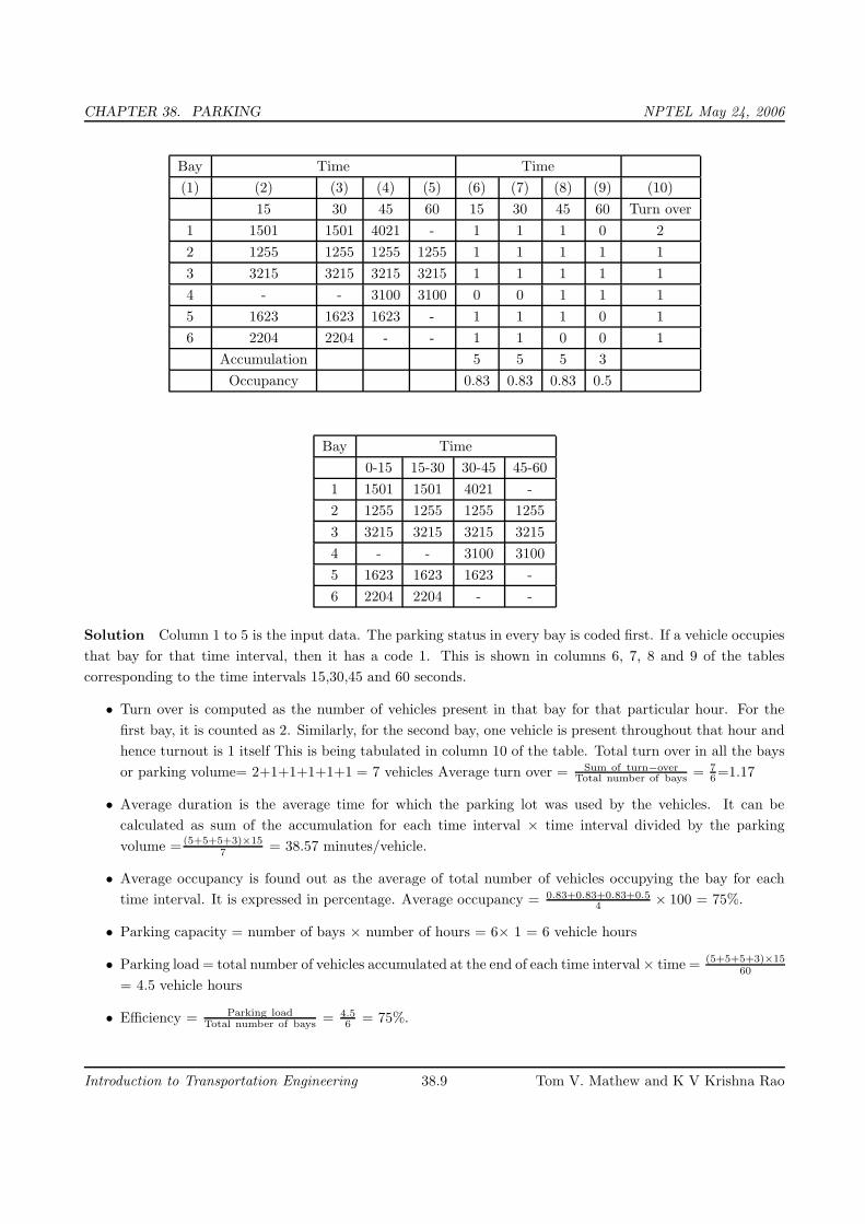
CHAPTER 38. PARKING NPTEL May 24, 2006
Bay Time Time
(1) (2) (3) (4) (5) (6) (7) (8) (9) (10)
15 30 45 60 15 30 45 60 Turn over
1 1501 1501 4021 - 1 1 1 0 2
2 1255 1255 1255 1255 1 1 1 1 1
3 3215 3215 3215 3215 1 1 1 1 1
4 - - 3100 3100 0 0 1 1 1
5 1623 1623 1623 - 1 1 1 0 1
6 2204 2204 - - 1 1 0 0 1
Accumulation 5 5 5 3
Occupancy 0.83 0.83 0.83 0.5
Bay Time
0-15 15-30 30-45 45-60
1 1501 1501 4021 -
2 1255 1255 1255 1255
3 3215 3215 3215 3215
4 - - 3100 3100
5 1623 1623 1623 -
6 2204 2204 - -
Solution Column 1 to 5 is the input data. The parking status in every bay is coded first. If a vehicle occupies
that bay for that time interval, then it has a code 1. This is shown in columns 6, 7, 8 and 9 of the tables
corresponding to the time intervals 15,30,45 and 60 seconds.
• Turn over is computed as the number of vehicles present in that bay for that particular hour. For the
first bay, it is counted as 2. Similarly, for the second bay, one vehicle is present throughout that hour and
hence turnout is 1 itself This is being tabulated in column 10 of the table. Total turn over in all the bays
or parking volume= 2+1+1+1+1+1 = 7 vehicles Average turn over = Sum of turn−over
Total number of bays= 7
6=1.17
• Average duration is the average time for which the parking lot was used by the vehicles. It can be
calculated as sum of the accumulation for each time interval × time interval divided by the parking
volume = (5+5+5+3)×15
7= 38.57 minutes/vehicle.
• Average occupancy is found out as the average of total number of vehicles occupying the bay for each
time interval. It is expressed in percentage. Average occupancy = 0.83+0.83+0.83+0.5
4× 100 = 75%.
• Parking capacity = number of bays × number of hours = 6× 1 = 6 vehicle hours
• Parking load = total number of vehicles accumulated at the end of each time interval× time = (5+5+5+3)×15
60
= 4.5 vehicle hours
• Efficiency = Parking load
Total number of bays= 4.5
6= 75%.
Introduction to Transportation Engineering 38.9 Tom V. Mathew and K V Krishna Rao
CHAPTER 39. TRAFFIC INTERSECTIONS NPTEL May 24, 2006
Chapter 39
Traffic intersections
39.1 Overview
Intersection is an area shared by two or more roads. This area is designated for the vehicles to turn to different
directions to reach their desired destinations. Its main function is to guide vehicles to their respective directions.
Traffic intersections are complex locations on any highway. This is because vehicles moving in different direction
wan to occupy same space at the same time. In addition, the pedestrians also seek same space for crossing.
Drivers have to make split second decision at an intersection by considering his route, intersection geometry,
speed and direction of other vehicles etc. A small error in judgment can cause severe accidents. It also causes
delay and it depends on type, geometry, and type of control. Overall traffic flow depends on the performance of
the intersections. It also affects the capacity of the road. Therefore, both from the accident perspective and the
capacity perspective, the study of intersections very important for the traffic engineers especially in the case of
urban scenario.
39.2 Conflicts at an intersection
Conflicts at an intersection are different for different types of intersection. Consider a typical four-legged
intersection as shown in figure. The number of conflicts for competing through movements are 4, while competing
right turn and through movements are 8. The conflicts between right turn traffics are 4, and between left turn and
merging traffic is 4. The conflicts created by pedestrians will be 8 taking into account all the four approaches.
Diverging traffic also produces about 4 conflicts. Therefore, a typical four legged intersection has about 32
different types of conflicts. This is shown in figure 39:1.
The essence of the intersection control is to resolve these conflicts at the intersection for the safe and efficient
movement of both vehicular traffic and pedestrians. Two methods of intersection controls are there: time sharing
and space sharing. The type of intersection control that has to be adopted depends on the traffic volume, road
geometry, cost involved, importance of the road etc.
39.3 Levels of intersection control
The control of an intersection can be exercised at different levels. They can be either passive control, semi
control, or active control. In passive control, there is no explicit control on the driver . In semi control, some
amount of control on the driver is there from the traffic agency. Active control means the movement of the
traffic is fully controlled by the traffic agency and the drivers cannot simply maneuver the intersection according
Introduction to Transportation Engineering 39.1 Tom V. Mathew and K V Krishna Rao
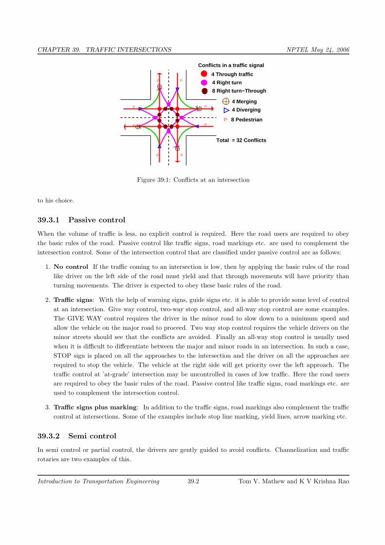
CHAPTER 39. TRAFFIC INTERSECTIONS NPTEL May 24, 2006
P
P
P P
P
P
PP
P 8 Pedestrian
Conflicts in a traffic signal
8 Right turn−Through
Total = 32 Conflicts
4 Merging
4 Right turn
4 Through traffic
4 Diverging
Figure 39:1: Conflicts at an intersection
to his choice.
39.3.1 Passive control
When the volume of traffic is less, no explicit control is required. Here the road users are required to obey
the basic rules of the road. Passive control like traffic signs, road markings etc. are used to complement the
intersection control. Some of the intersection control that are classified under passive control are as follows:
1. No control If the traffic coming to an intersection is low, then by applying the basic rules of the road
like driver on the left side of the road must yield and that through movements will have priority than
turning movements. The driver is expected to obey these basic rules of the road.
2. Traffic signs: With the help of warning signs, guide signs etc. it is able to provide some level of control
at an intersection. Give way control, two-way stop control, and all-way stop control are some examples.
The GIVE WAY control requires the driver in the minor road to slow down to a minimum speed and
allow the vehicle on the major road to proceed. Two way stop control requires the vehicle drivers on the
minor streets should see that the conflicts are avoided. Finally an all-way stop control is usually used
when it is difficult to differentiate between the major and minor roads in an intersection. In such a case,
STOP sign is placed on all the approaches to the intersection and the driver on all the approaches are
required to stop the vehicle. The vehicle at the right side will get priority over the left approach. The
traffic control at ’at-grade’ intersection may be uncontrolled in cases of low traffic. Here the road users
are required to obey the basic rules of the road. Passive control like traffic signs, road markings etc. are
used to complement the intersection control.
3. Traffic signs plus marking: In addition to the traffic signs, road markings also complement the traffic
control at intersections. Some of the examples include stop line marking, yield lines, arrow marking etc.
39.3.2 Semi control
In semi control or partial control, the drivers are gently guided to avoid conflicts. Channelization and traffic
rotaries are two examples of this.
Introduction to Transportation Engineering 39.2 Tom V. Mathew and K V Krishna Rao
CHAPTER 39. TRAFFIC INTERSECTIONS NPTEL May 24, 2006
1. Channelization: The traffic is separated to flow through definite paths by raising a portion of the road
in the middle usually called as islands distinguished by road markings. The conflicts in traffic movements
are reduced to a great extent in such a case. In channelized intersections, as the name suggests, the traffic
is directed to flow through different channels and this physical separation is made possible with the help
of some barriers in the road like traffic islands, road markings etc.
2. Traffic rotaries: It is a form of intersection control in which the traffic is made to flow along one
direction around a traffic island. The essential principle of this control is to convert all the severe conflicts
like through and right turn conflicts into milder conflicts like merging, weaving and diverging. It is a
form of ‘at-grade’ intersection laid out for the movement of traffic such that no through conflicts are there.
Free-left turn is permitted where as through traffic and right-turn traffic is forced to move around the
central island in a clock-wise direction in an orderly manner. Merging, weaving and diverging operations
reduces the conflicting movements at the rotary.
39.3.3 Active control
Active control implies that the road user will be forced to follow the path suggested by the traffic control
agencies. He cannot maneuver according to his wish. Traffic signals and grade separated intersections come
under this classification.
1. Traffic signals: Control using traffic signal is based on time sharing approach. At a given time, with the
help of appropriate signals, certain traffic movements are restricted where as certain other movements are
permitted to pass through the intersection. Two or more phases may be provided depending upon the
traffic conditions of the intersection. When the vehicles traversing the intersection is very large, then the
control is done with the help of signals. The phases provided for the signal may be two or more. If more
than two phases are provided, then it is called multiphase signal.
The signals can operate in several modes. Most common are fixed time signals and vehicle actuated
signals. In fixed time signals, the cycle time, phases and interval of each signal is fixed. Each cycle of the
signal will be exactly like another. But they cannot cater to the needs of the fluctuating traffic. On the
other hand, vehicle actuated signals can respond to dynamic traffic situations. Vehicle detectors will be
placed on the streets approaching the intersection and the detector will sense the presence of the vehicle
and pass the information to a controller. The controller then sets the cycle time and adjusts the phase
lengths according to the prevailing traffic conditions.
2. Grade separated intersections: The intersections are of two types. They are at-grade intersections
and grade-separated intersections. In at-grade intersections, all roadways join or cross at the same vertical
level. Grade separated intersections allows the traffic to cross at different vertical levels. Sometimes the
topography itself may be helpful in constructing such intersections. Otherwise, the initial construction
cost required will be very high. Therefore, they are usually constructed on high speed facilities like
expressways, freeways etc. These type of intersection increases the road capacity because vehicles can flow
with high speed and accident potential is also reduced due to vertical separation of traffic.
Introduction to Transportation Engineering 39.3 Tom V. Mathew and K V Krishna Rao
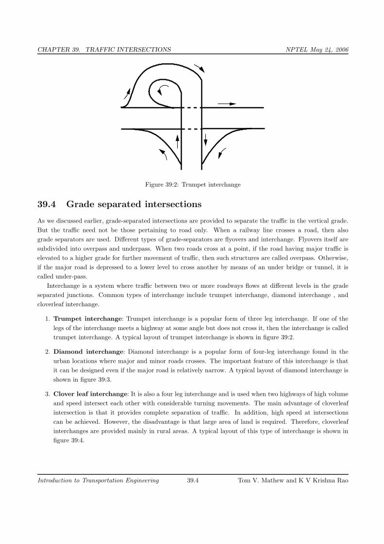
CHAPTER 39. TRAFFIC INTERSECTIONS NPTEL May 24, 2006
Figure 39:2: Trumpet interchange
39.4 Grade separated intersections
As we discussed earlier, grade-separated intersections are provided to separate the traffic in the vertical grade.
But the traffic need not be those pertaining to road only. When a railway line crosses a road, then also
grade separators are used. Different types of grade-separators are flyovers and interchange. Flyovers itself are
subdivided into overpass and underpass. When two roads cross at a point, if the road having major traffic is
elevated to a higher grade for further movement of traffic, then such structures are called overpass. Otherwise,
if the major road is depressed to a lower level to cross another by means of an under bridge or tunnel, it is
called under-pass.
Interchange is a system where traffic between two or more roadways flows at different levels in the grade
separated junctions. Common types of interchange include trumpet interchange, diamond interchange , and
cloverleaf interchange.
1. Trumpet interchange: Trumpet interchange is a popular form of three leg interchange. If one of the
legs of the interchange meets a highway at some angle but does not cross it, then the interchange is called
trumpet interchange. A typical layout of trumpet interchange is shown in figure 39:2.
2. Diamond interchange: Diamond interchange is a popular form of four-leg interchange found in the
urban locations where major and minor roads crosses. The important feature of this interchange is that
it can be designed even if the major road is relatively narrow. A typical layout of diamond interchange is
shown in figure 39:3.
3. Clover leaf interchange: It is also a four leg interchange and is used when two highways of high volume
and speed intersect each other with considerable turning movements. The main advantage of cloverleaf
intersection is that it provides complete separation of traffic. In addition, high speed at intersections
can be achieved. However, the disadvantage is that large area of land is required. Therefore, cloverleaf
interchanges are provided mainly in rural areas. A typical layout of this type of interchange is shown in
figure 39:4.
Introduction to Transportation Engineering 39.4 Tom V. Mathew and K V Krishna Rao
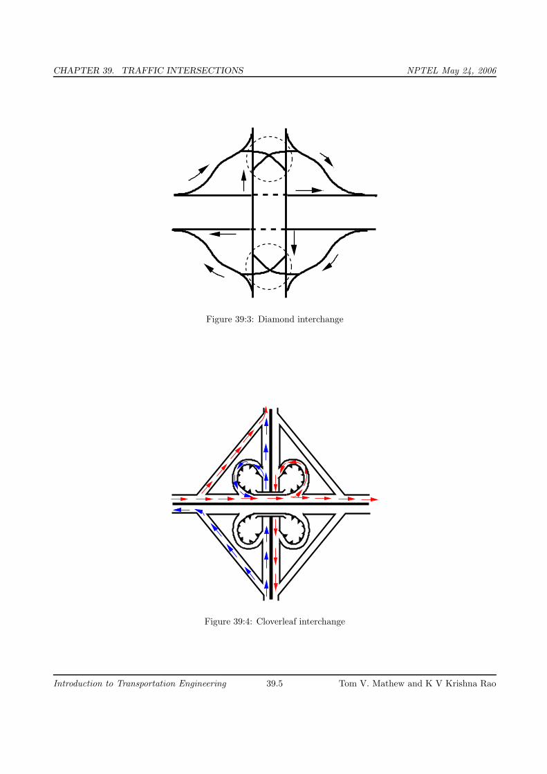
CHAPTER 39. TRAFFIC INTERSECTIONS NPTEL May 24, 2006
Figure 39:3: Diamond interchange
����
����
��������
������������
����
� � ��
����
����
������
����
������
��������
������
��� � !!""#�##�#$
$
%%&&
'()�))�))�)*�**�**�*+,
-.//00 111222
3344
5566 7788
Figure 39:4: Cloverleaf interchange
Introduction to Transportation Engineering 39.5 Tom V. Mathew and K V Krishna Rao
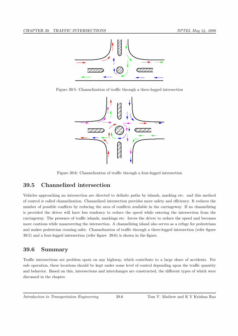
CHAPTER 39. TRAFFIC INTERSECTIONS NPTEL May 24, 2006
���������������������������������������������
���������������������������������������������
����������������������������������������������������������������������
��������������������������������������������������
������������������������������������������������������������������������������������
����������������������������������������������������������������������������
���������������������������������������������������������������
���������������������������������������������������������������
Figure 39:5: Channelization of traffic through a three-legged intersection
������������������������������������
���������������������������������
������������������������������
������������������������������
������������������������������
������������������������������
��������������������������������������������
���������������������������������
Figure 39:6: Channelization of traffic through a four-legged intersection
39.5 Channelized intersection
Vehicles approaching an intersection are directed to definite paths by islands, marking etc. and this method
of control is called channelization. Channelized intersection provides more safety and efficiency. It reduces the
number of possible conflicts by reducing the area of conflicts available in the carriageway. If no channelizing
is provided the driver will have less tendency to reduce the speed while entering the intersection from the
carriageway. The presence of traffic islands, markings etc. forces the driver to reduce the speed and becomes
more cautious while maneuvering the intersection. A channelizing island also serves as a refuge for pedestrians
and makes pedestrian crossing safer. Channelization of traffic through a three-legged intersection (refer figure
39:5) and a four-legged intersection (refer figure 39:6) is shown in the figure.
39.6 Summary
Traffic intersections are problem spots on any highway, which contribute to a large share of accidents. For
safe operation, these locations should be kept under some level of control depending upon the traffic quantity
and behavior. Based on this, intersections and interchanges are constructed, the different types of which were
discussed in the chapter.
Introduction to Transportation Engineering 39.6 Tom V. Mathew and K V Krishna Rao
CHAPTER 39. TRAFFIC INTERSECTIONS NPTEL May 24, 2006
39.7 Problems
1. The GIVE WAY control
(a) requires the driver in the minor road to slow down to a minimum speed and allow the vehicle on the
major road to proceed.
(b) requires the driver in the major road to slow down to a minimum speed and allow the vehicle on the
minor road to proceed.
(c) requires the drivers on both minor and major roads to stop.
(d) is similar to one way control.
2. Traffic signal is an example of
(a) Passive control
(b) No control
(c) Active control
(d) none of these
39.8 Solutions
1. The GIVE WAY control
(a) requires the driver in the minor road to slow down to a minimum speed and allow the vehicle on the
major road to proceed.√
(b) requires the driver in the major road to slow down to a minimum speed and allow the vehicle on the
minor road to proceed.
(c) requires the drivers on both minor and major roads to stop.
(d) is similar to one way control.
2. Traffic signal is an example of
(a) Passive control
(b) No control
(c) Active control√
(d) none of these
Introduction to Transportation Engineering 39.7 Tom V. Mathew and K V Krishna Rao
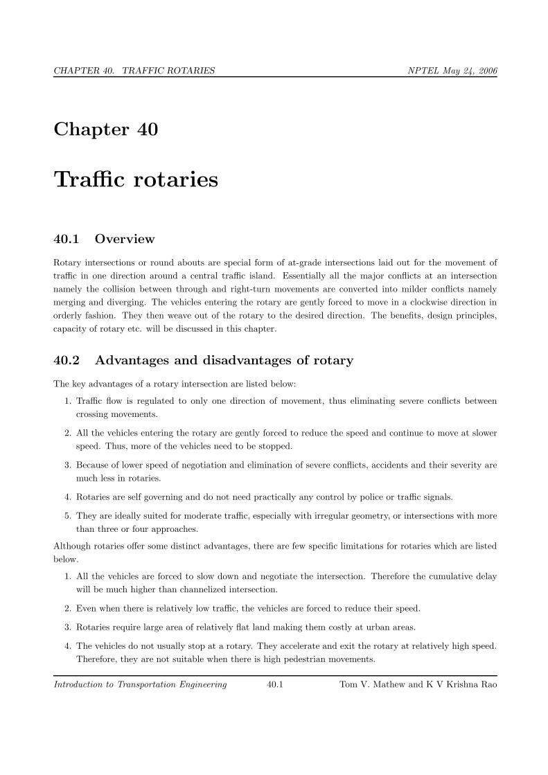
CHAPTER 40. TRAFFIC ROTARIES NPTEL May 24, 2006
Chapter 40
Traffic rotaries
40.1 Overview
Rotary intersections or round abouts are special form of at-grade intersections laid out for the movement of
traffic in one direction around a central traffic island. Essentially all the major conflicts at an intersection
namely the collision between through and right-turn movements are converted into milder conflicts namely
merging and diverging. The vehicles entering the rotary are gently forced to move in a clockwise direction in
orderly fashion. They then weave out of the rotary to the desired direction. The benefits, design principles,
capacity of rotary etc. will be discussed in this chapter.
40.2 Advantages and disadvantages of rotary
The key advantages of a rotary intersection are listed below:
1. Traffic flow is regulated to only one direction of movement, thus eliminating severe conflicts between
crossing movements.
2. All the vehicles entering the rotary are gently forced to reduce the speed and continue to move at slower
speed. Thus, more of the vehicles need to be stopped.
3. Because of lower speed of negotiation and elimination of severe conflicts, accidents and their severity are
much less in rotaries.
4. Rotaries are self governing and do not need practically any control by police or traffic signals.
5. They are ideally suited for moderate traffic, especially with irregular geometry, or intersections with more
than three or four approaches.
Although rotaries offer some distinct advantages, there are few specific limitations for rotaries which are listed
below.
1. All the vehicles are forced to slow down and negotiate the intersection. Therefore the cumulative delay
will be much higher than channelized intersection.
2. Even when there is relatively low traffic, the vehicles are forced to reduce their speed.
3. Rotaries require large area of relatively flat land making them costly at urban areas.
4. The vehicles do not usually stop at a rotary. They accelerate and exit the rotary at relatively high speed.
Therefore, they are not suitable when there is high pedestrian movements.
Introduction to Transportation Engineering 40.1 Tom V. Mathew and K V Krishna Rao
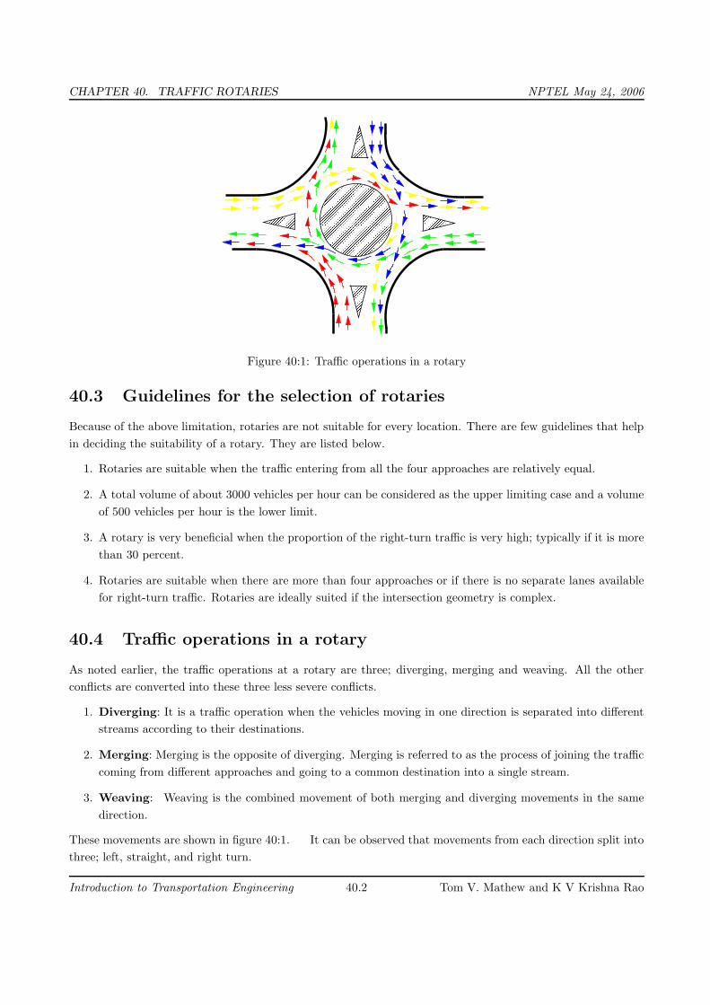
CHAPTER 40. TRAFFIC ROTARIES NPTEL May 24, 2006
���������������������������������������������������������������������������������������������������������������������������������������������������������������������������������������������������������������������������������������������������������������������������������������������������������������������������������������������������������������������������������������������������������������������������������������������������
���������������������������������������������������������������������������������������������������������������������������������������������������������������������������������������������������������������������������������������������������������������������������������������������������������������������������������������������������������������������������������������������������������������������������������������������������
������������������������������������������������������������
����������������������������������������������������
�������������������������������������������������
�������������������������������������������������
������������������������������������������������������������
������������������������������������������������������������
����������������������������
����������������������������
Figure 40:1: Traffic operations in a rotary
40.3 Guidelines for the selection of rotaries
Because of the above limitation, rotaries are not suitable for every location. There are few guidelines that help
in deciding the suitability of a rotary. They are listed below.
1. Rotaries are suitable when the traffic entering from all the four approaches are relatively equal.
2. A total volume of about 3000 vehicles per hour can be considered as the upper limiting case and a volume
of 500 vehicles per hour is the lower limit.
3. A rotary is very beneficial when the proportion of the right-turn traffic is very high; typically if it is more
than 30 percent.
4. Rotaries are suitable when there are more than four approaches or if there is no separate lanes available
for right-turn traffic. Rotaries are ideally suited if the intersection geometry is complex.
40.4 Traffic operations in a rotary
As noted earlier, the traffic operations at a rotary are three; diverging, merging and weaving. All the other
conflicts are converted into these three less severe conflicts.
1. Diverging: It is a traffic operation when the vehicles moving in one direction is separated into different
streams according to their destinations.
2. Merging: Merging is the opposite of diverging. Merging is referred to as the process of joining the traffic
coming from different approaches and going to a common destination into a single stream.
3. Weaving: Weaving is the combined movement of both merging and diverging movements in the same
direction.
These movements are shown in figure 40:1. It can be observed that movements from each direction split into
three; left, straight, and right turn.
Introduction to Transportation Engineering 40.2 Tom V. Mathew and K V Krishna Rao
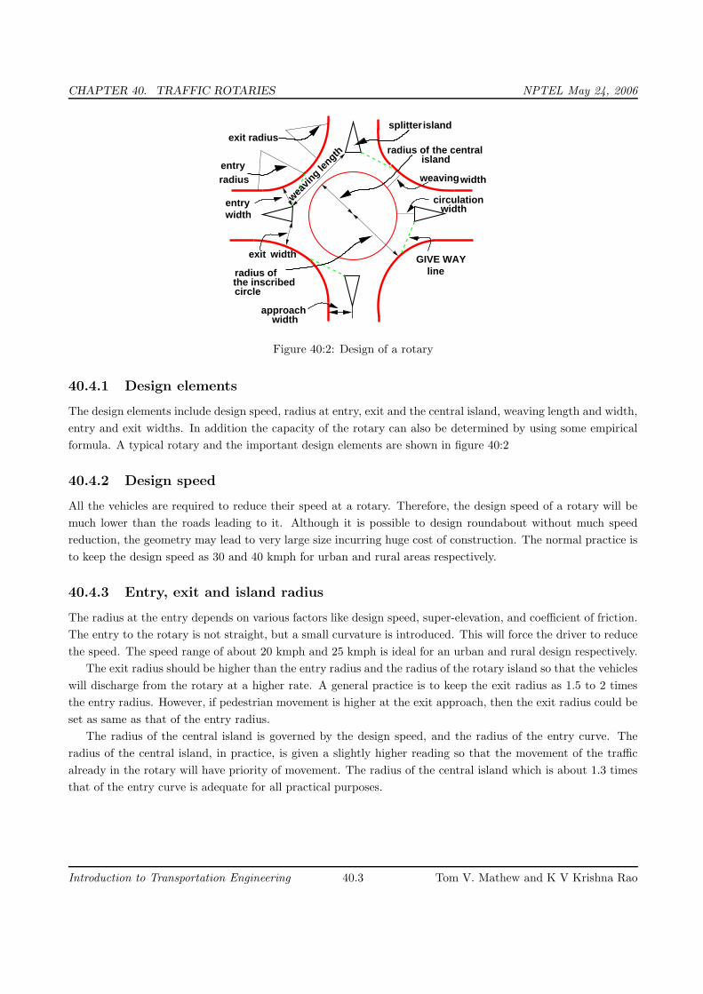
CHAPTER 40. TRAFFIC ROTARIES NPTEL May 24, 2006
splitterisland
the inscribed circle
radius of
entry
exit radius
radius
entrywidth
circulation width
weavin
g length
GIVE WAY line
approachwidth
widthexit
weavingwidth
radius of the centralisland
Figure 40:2: Design of a rotary
40.4.1 Design elements
The design elements include design speed, radius at entry, exit and the central island, weaving length and width,
entry and exit widths. In addition the capacity of the rotary can also be determined by using some empirical
formula. A typical rotary and the important design elements are shown in figure 40:2
40.4.2 Design speed
All the vehicles are required to reduce their speed at a rotary. Therefore, the design speed of a rotary will be
much lower than the roads leading to it. Although it is possible to design roundabout without much speed
reduction, the geometry may lead to very large size incurring huge cost of construction. The normal practice is
to keep the design speed as 30 and 40 kmph for urban and rural areas respectively.
40.4.3 Entry, exit and island radius
The radius at the entry depends on various factors like design speed, super-elevation, and coefficient of friction.
The entry to the rotary is not straight, but a small curvature is introduced. This will force the driver to reduce
the speed. The speed range of about 20 kmph and 25 kmph is ideal for an urban and rural design respectively.
The exit radius should be higher than the entry radius and the radius of the rotary island so that the vehicles
will discharge from the rotary at a higher rate. A general practice is to keep the exit radius as 1.5 to 2 times
the entry radius. However, if pedestrian movement is higher at the exit approach, then the exit radius could be
set as same as that of the entry radius.
The radius of the central island is governed by the design speed, and the radius of the entry curve. The
radius of the central island, in practice, is given a slightly higher reading so that the movement of the traffic
already in the rotary will have priority of movement. The radius of the central island which is about 1.3 times
that of the entry curve is adequate for all practical purposes.
Introduction to Transportation Engineering 40.3 Tom V. Mathew and K V Krishna Rao
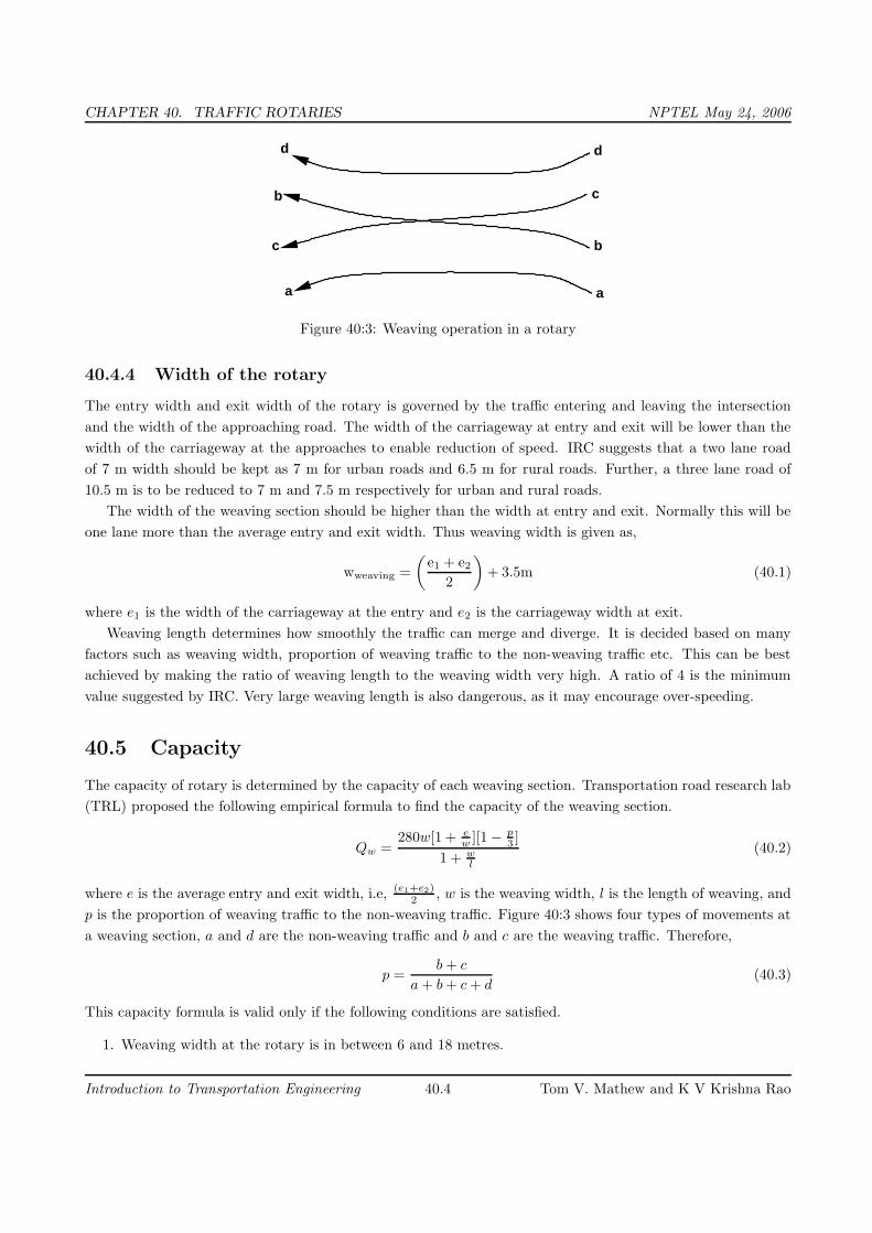
CHAPTER 40. TRAFFIC ROTARIES NPTEL May 24, 2006
d
b
c
a
d
c
b
a
Figure 40:3: Weaving operation in a rotary
40.4.4 Width of the rotary
The entry width and exit width of the rotary is governed by the traffic entering and leaving the intersection
and the width of the approaching road. The width of the carriageway at entry and exit will be lower than the
width of the carriageway at the approaches to enable reduction of speed. IRC suggests that a two lane road
of 7 m width should be kept as 7 m for urban roads and 6.5 m for rural roads. Further, a three lane road of
10.5 m is to be reduced to 7 m and 7.5 m respectively for urban and rural roads.
The width of the weaving section should be higher than the width at entry and exit. Normally this will be
one lane more than the average entry and exit width. Thus weaving width is given as,
wweaving =
(
e1 + e2
2
)
+ 3.5m (40.1)
where e1 is the width of the carriageway at the entry and e2 is the carriageway width at exit.
Weaving length determines how smoothly the traffic can merge and diverge. It is decided based on many
factors such as weaving width, proportion of weaving traffic to the non-weaving traffic etc. This can be best
achieved by making the ratio of weaving length to the weaving width very high. A ratio of 4 is the minimum
value suggested by IRC. Very large weaving length is also dangerous, as it may encourage over-speeding.
40.5 Capacity
The capacity of rotary is determined by the capacity of each weaving section. Transportation road research lab
(TRL) proposed the following empirical formula to find the capacity of the weaving section.
Qw =280w[1 + e
w][1 −
p
3]
1 + w
l
(40.2)
where e is the average entry and exit width, i.e, (e1+e2)
2, w is the weaving width, l is the length of weaving, and
p is the proportion of weaving traffic to the non-weaving traffic. Figure 40:3 shows four types of movements at
a weaving section, a and d are the non-weaving traffic and b and c are the weaving traffic. Therefore,
p =b + c
a + b + c + d(40.3)
This capacity formula is valid only if the following conditions are satisfied.
1. Weaving width at the rotary is in between 6 and 18 metres.
Introduction to Transportation Engineering 40.4 Tom V. Mathew and K V Krishna Rao
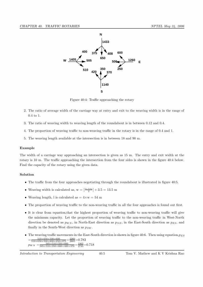
CHAPTER 40. TRAFFIC ROTARIES NPTEL May 24, 2006
1405
400
505
510
375 408650
500
600
250
1260
1140
420350
370
1433
N
EW
S
Figure 40:4: Traffic approaching the rotary
2. The ratio of average width of the carriage way at entry and exit to the weaving width is in the range of
0.4 to 1.
3. The ratio of weaving width to weaving length of the roundabout is in between 0.12 and 0.4.
4. The proportion of weaving traffic to non-weaving traffic in the rotary is in the range of 0.4 and 1.
5. The weaving length available at the intersection is in between 18 and 90 m.
Example
The width of a carriage way approaching an intersection is given as 15 m. The entry and exit width at the
rotary is 10 m. The traffic approaching the intersection from the four sides is shown in the figure 40:4 below.
Find the capacity of the rotary using the given data.
Solution
• The traffic from the four approaches negotiating through the roundabout is illustrated in figure 40:5.
• Weaving width is calculated as, w = [ e1+e2
2] + 3.5 = 13.5 m
• Weaving length, l is calculated as = 4×w = 54 m
• The proportion of weaving traffic to the non-weaving traffic in all the four approaches is found out first.
• It is clear from equation,that the highest proportion of weaving traffic to non-weaving traffic will give
the minimum capacity. Let the proportion of weaving traffic to the non-weaving traffic in West-North
direction be denoted as pWN , in North-East direction as pNE , in the East-South direction as pES, and
finally in the South-West direction as pSW .
• The weaving traffic movements in the East-South direction is shown in figure 40:6. Then using equation,pES
= 510+650+500+600
510+650+500+600+250+375= 2260
2885=0.783
pWN = 505+510+350+600
505+510+350+600+400+370= 1965
2735=0.718
Introduction to Transportation Engineering 40.5 Tom V. Mathew and K V Krishna Rao
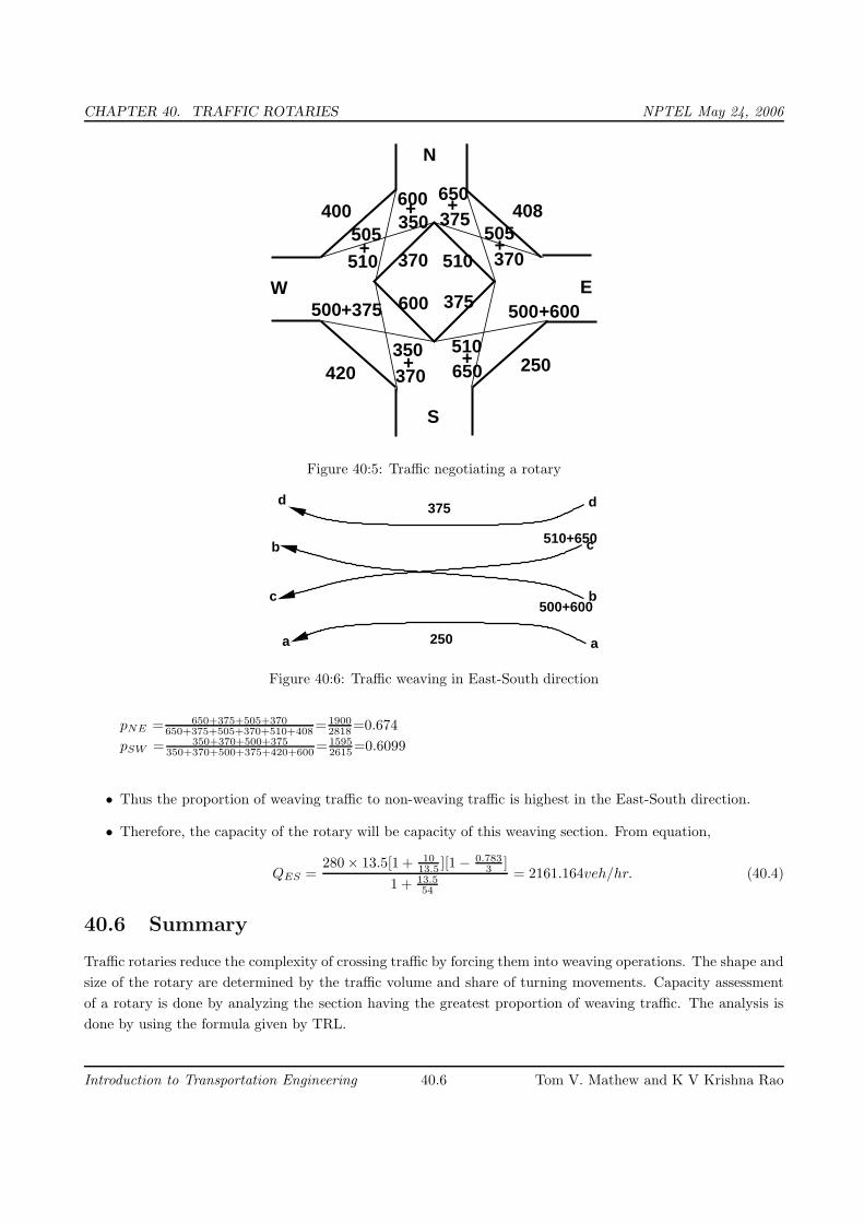
CHAPTER 40. TRAFFIC ROTARIES NPTEL May 24, 2006
505
500
350 510650+
370+
600 350
+650+
370+
420
400
250
408
E
N
S
W
370 510
600 375 500
510505+
+375 +600
375
Figure 40:5: Traffic negotiating a rotary
d
b
c
a
d
c
b
a
375
250
510+650
500+600
Figure 40:6: Traffic weaving in East-South direction
pNE = 650+375+505+370
650+375+505+370+510+408= 1900
2818=0.674
pSW = 350+370+500+375
350+370+500+375+420+600= 1595
2615=0.6099
• Thus the proportion of weaving traffic to non-weaving traffic is highest in the East-South direction.
• Therefore, the capacity of the rotary will be capacity of this weaving section. From equation,
QES =280× 13.5[1 + 10
13.5][1 − 0.783
3]
1 + 13.5
54
= 2161.164veh/hr. (40.4)
40.6 Summary
Traffic rotaries reduce the complexity of crossing traffic by forcing them into weaving operations. The shape and
size of the rotary are determined by the traffic volume and share of turning movements. Capacity assessment
of a rotary is done by analyzing the section having the greatest proportion of weaving traffic. The analysis is
done by using the formula given by TRL.
Introduction to Transportation Engineering 40.6 Tom V. Mathew and K V Krishna Rao
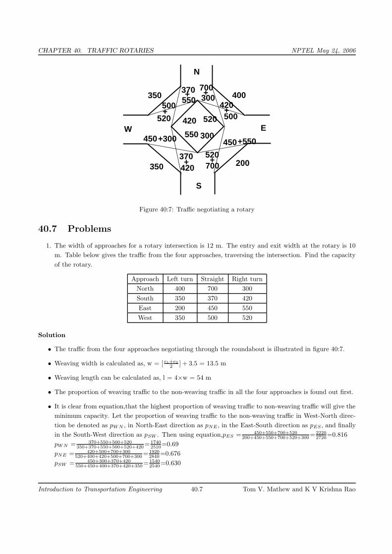
CHAPTER 40. TRAFFIC ROTARIES NPTEL May 24, 2006
420500
520 520
450+550300450
370
420
550+300
520700+
420+
550+
700 300
+
+ 500+
350
350
200
400370
W E
S
N
Figure 40:7: Traffic negotiating a rotary
40.7 Problems
1. The width of approaches for a rotary intersection is 12 m. The entry and exit width at the rotary is 10
m. Table below gives the traffic from the four approaches, traversing the intersection. Find the capacity
of the rotary.
Approach Left turn Straight Right turn
North 400 700 300
South 350 370 420
East 200 450 550
West 350 500 520
Solution
• The traffic from the four approaches negotiating through the roundabout is illustrated in figure 40:7.
• Weaving width is calculated as, w = [ e1+e2
2] + 3.5 = 13.5 m
• Weaving length can be calculated as, l = 4×w = 54 m
• The proportion of weaving traffic to the non-weaving traffic in all the four approaches is found out first.
• It is clear from equation,that the highest proportion of weaving traffic to non-weaving traffic will give the
minimum capacity. Let the proportion of weaving traffic to the non-weaving traffic in West-North direc-
tion be denoted as pWN , in North-East direction as pNE , in the East-South direction as pES , and finally
in the South-West direction as pSW . Then using equation,pES = 450+550+700+520
200+450+550+700+520+300= 2220
2720=0.816
pWN = 370+550+500+520
350+370+550+500+520+420= 1740
2510=0.69
pNE = 420+500+700+300
520+400+420+500+700+300= 1920
2840=0.676
pSW = 450+300+370+420
550+450+400+370+420+350= 1540
2540=0.630
Introduction to Transportation Engineering 40.7 Tom V. Mathew and K V Krishna Rao
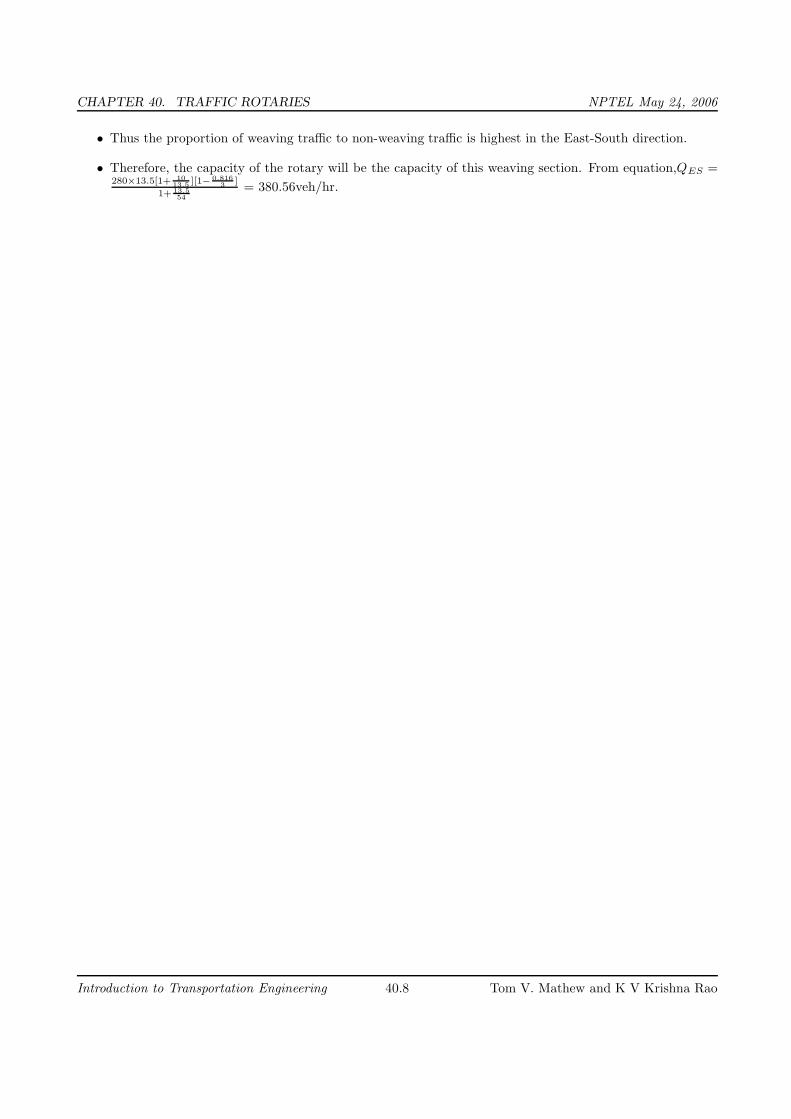
CHAPTER 40. TRAFFIC ROTARIES NPTEL May 24, 2006
• Thus the proportion of weaving traffic to non-weaving traffic is highest in the East-South direction.
• Therefore, the capacity of the rotary will be the capacity of this weaving section. From equation,QES =280×13.5[1+
10
13.5][1−
0.816
3]
1+13.5
54
= 380.56veh/hr.
Introduction to Transportation Engineering 40.8 Tom V. Mathew and K V Krishna Rao
CHAPTER 41. TRAFFIC SIGNAL DESIGN-I NPTEL May 24, 2006
Chapter 41
Traffic signal design-I
41.1 Overview
The conflicts arising from movements of traffic in different directions is solved by time sharing of the principle.
The advantages of traffic signal includes an orderly movement of traffic, an increased capacity of the intersection
and requires only simple geometric design. However the disadvantages of the signalized intersection are it affects
larger stopped delays, and the design requires complex considerations. Although the overall delay may be lesser
than a rotary for a high volume, a user is more concerned about the stopped delay.
41.2 Definitions and notations
A number of definitions and notations need to be understood in signal design. They are discussed below:
• Cycle: A signal cycle is one complete rotation through all of the indications provided.
• Cycle length: Cycle length is the time in seconds that it takes a signal to complete one full cycle of
indications. It indicates the time interval between the starting of of green for one approach till the next
time the green starts. It is denoted by C.
• Interval: Thus it indicates the change from one stage to another. There are two types of intervals -
change interval and clearance interval. Change interval is also called the yellow time indicates the interval
between the green and red signal indications for an approach. Clearance interval is also called all red is
included after each yellow interval indicating a period during which all signal faces show red and is used
for clearing off the vehicles in the intersection.
• Green interval: It is the green indication for a particular movement or set of movements and is denoted
by Gi. This is the actual duration the green light of a traffic signal is turned on.
• Red interval: It is the red indication for a particular movement or set of movements and is denoted by
Ri. This is the actual duration the red light of a traffic signal is turned on.
• Phase: A phase is the green interval plus the change and clearance intervals that follow it. Thus, during
green interval, non conflicting movements are assigned into each phase. It allows a set of movements to
flow and safely halt the flow before the phase of another set of movements start.
• Lost time: It indicates the time during which the intersection is not effectively utilized for any movement.
For example, when the signal for an approach turns from red to green, the driver of the vehicle which is
Introduction to Transportation Engineering 41.1 Tom V. Mathew and K V Krishna Rao
CHAPTER 41. TRAFFIC SIGNAL DESIGN-I NPTEL May 24, 2006
1
5
3
7
2
64
8
Figure 41:1: Four legged intersection
in the front of the queue, will take some time to perceive the signal (usually called as reaction time) and
some time will be lost here before he moves.
41.3 Phase design
The signal design procedure involves six major steps. They include the (1) phase design, (2) determination of
amber time and clearance time, (3) determination of cycle length, (4)apportioning of green time, (5) pedestrian
crossing requirements, and (6) the performance evaluation of the above design. The objective of phase design
is to separate the conflicting movements in an intersection into various phases, so that movements in a phase
should have no conflicts. If all the movements are to be separated with no conflicts, then a large number of
phases are required. In such a situation, the objective is to design phases with minimum conflicts or with less
severe conflicts.
There is no precise methodology for the design of phases. This is often guided by the geometry of the
intersection, flow pattern especially the turning movements, the relative magnitudes of flow. Therefore, a trial
and error procedure is often adopted. However, phase design is very important because it affects the further
design steps. Further, it is easier to change the cycle time and green time when flow pattern changes, where as
a drastic change in the flow pattern may cause considerable confusion to the drivers. To illustrate various phase
plan options, consider a four legged intersection with through traffic and right turns. Left turn is ignored. See
figure 41:1. The first issue is to decide how many phases are required. It is possible to have two, three, four or
even more number of phases.
41.3.1 Two phase signals
Two phase system is usually adopted if through traffic is significant compared to the turning movements. For
example in figure 41:2, non-conflicting through traffic 3 and 4 are grouped in a single phase and non-conflicting
through traffic 1 and 2 are grouped in the second phase. However, in the first phase flow 7 and 8 offer some
conflicts and are called permitted right turns. Needless to say that such phasing is possible only if the turning
Introduction to Transportation Engineering 41.2 Tom V. Mathew and K V Krishna Rao
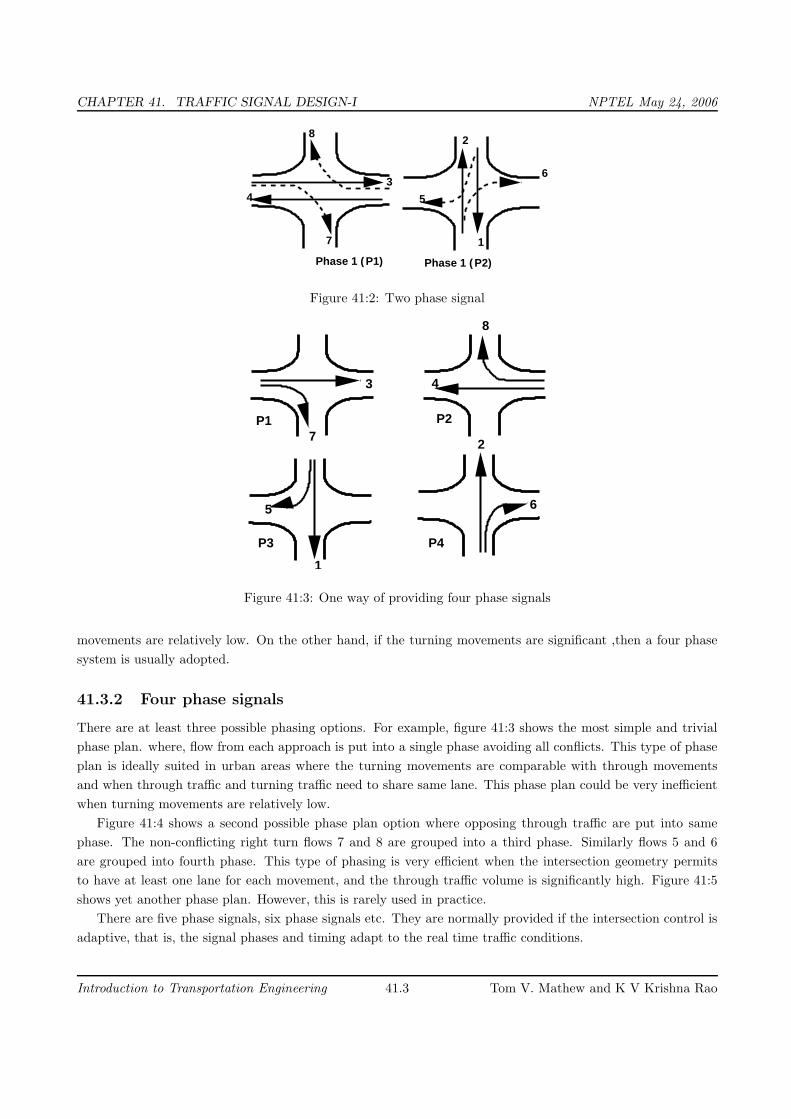
CHAPTER 41. TRAFFIC SIGNAL DESIGN-I NPTEL May 24, 2006
Phase 1 ( P1) Phase 1 ( P2)
2
5
6
1
4
8
3
7
Figure 41:2: Two phase signal
73
7
8
4
5
1
6
2
P1 P2
P3 P4
Figure 41:3: One way of providing four phase signals
movements are relatively low. On the other hand, if the turning movements are significant ,then a four phase
system is usually adopted.
41.3.2 Four phase signals
There are at least three possible phasing options. For example, figure 41:3 shows the most simple and trivial
phase plan. where, flow from each approach is put into a single phase avoiding all conflicts. This type of phase
plan is ideally suited in urban areas where the turning movements are comparable with through movements
and when through traffic and turning traffic need to share same lane. This phase plan could be very inefficient
when turning movements are relatively low.
Figure 41:4 shows a second possible phase plan option where opposing through traffic are put into same
phase. The non-conflicting right turn flows 7 and 8 are grouped into a third phase. Similarly flows 5 and 6
are grouped into fourth phase. This type of phasing is very efficient when the intersection geometry permits
to have at least one lane for each movement, and the through traffic volume is significantly high. Figure 41:5
shows yet another phase plan. However, this is rarely used in practice.
There are five phase signals, six phase signals etc. They are normally provided if the intersection control is
adaptive, that is, the signal phases and timing adapt to the real time traffic conditions.
Introduction to Transportation Engineering 41.3 Tom V. Mathew and K V Krishna Rao
CHAPTER 41. TRAFFIC SIGNAL DESIGN-I NPTEL May 24, 2006
7
6
43
1
5
7
8
2
P1 P2
P3 P4
Figure 41:4: Second possible way of providing a four phase signal
3
1
6 4
2 8
5
7
P1P2
P3 P4
Figure 41:5: Third possible way of providing a four-phase signal
Introduction to Transportation Engineering 41.4 Tom V. Mathew and K V Krishna Rao
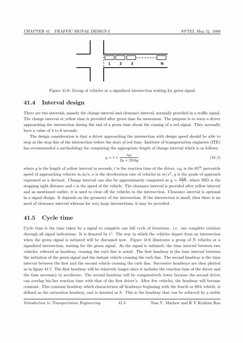
CHAPTER 41. TRAFFIC SIGNAL DESIGN-I NPTEL May 24, 2006
1 32 N
Figure 41:6: Group of vehicles at a signalized intersection waiting for green signal
41.4 Interval design
There are two intervals, namely the change interval and clearance interval, normally provided in a traffic signal.
The change interval or yellow time is provided after green time for movement. The purpose is to warn a driver
approaching the intersection during the end of a green time about the coming of a red signal. They normally
have a value of 3 to 6 seconds.
The design consideration is that a driver approaching the intersection with design speed should be able to
stop at the stop line of the intersection before the start of red time. Institute of transportation engineers (ITE)
has recommended a methodology for computing the appropriate length of change interval which is as follows:
y = t +v85
2a + 19.6g(41.1)
where y is the length of yellow interval in seconds, t is the reaction time of the driver, v85 is the 85th percentile
speed of approaching vehicles in m/s, a is the deceleration rate of vehicles in m/s2, g is the grade of approach
expressed as a decimal. Change interval can also be approximately computed as y = SSD
v, where SSD is the
stopping sight distance and v is the speed of the vehicle. The clearance interval is provided after yellow interval
and as mentioned earlier, it is used to clear off the vehicles in the intersection. Clearance interval is optional
in a signal design. It depends on the geometry of the intersection. If the intersection is small, then there is no
need of clearance interval whereas for very large intersections, it may be provided.
41.5 Cycle time
Cycle time is the time taken by a signal to complete one full cycle of iterations. i.e. one complete rotation
through all signal indications. It is denoted by C. The way in which the vehicles depart from an intersection
when the green signal is initiated will be discussed now. Figure 41:6 illustrates a group of N vehicles at a
signalized intersection, waiting for the green signal. As the signal is initiated, the time interval between two
vehicles, referred as headway, crossing the curb line is noted. The first headway is the time interval between
the initiation of the green signal and the instant vehicle crossing the curb line. The second headway is the time
interval between the first and the second vehicle crossing the curb line. Successive headways are then plotted
as in figure 41:7. The first headway will be relatively longer since it includes the reaction time of the driver and
the time necessary to accelerate. The second headway will be comparatively lower because the second driver
can overlap his/her reaction time with that of the first driver’s. After few vehicles, the headway will become
constant. This constant headway which characterizes all headways beginning with the fourth or fifth vehicle, is
defined as the saturation headway, and is denoted as h. This is the headway that can be achieved by a stable
Introduction to Transportation Engineering 41.5 Tom V. Mathew and K V Krishna Rao
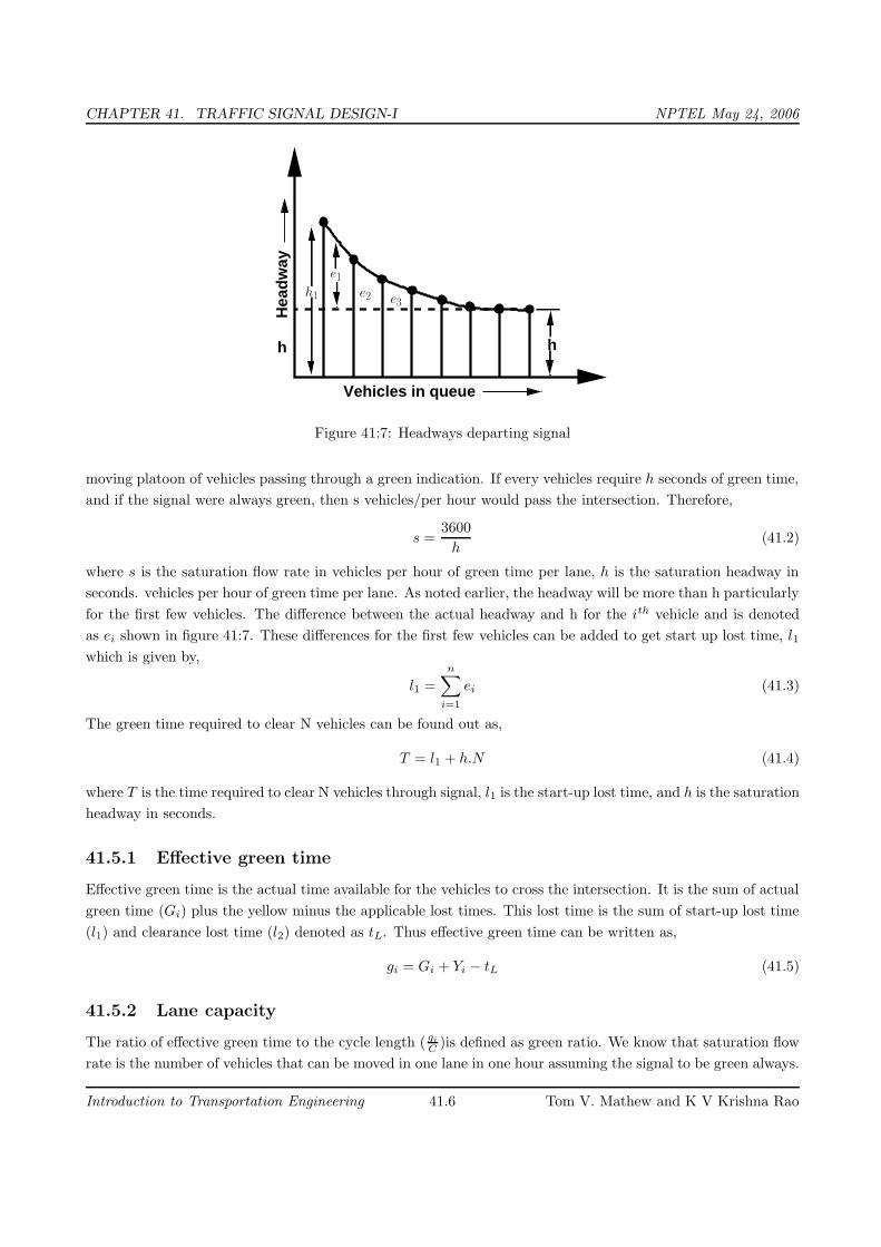
CHAPTER 41. TRAFFIC SIGNAL DESIGN-I NPTEL May 24, 2006
Vehicles in queue
h
Hea
dw
ay
h
e1
e2 e3
h1
Figure 41:7: Headways departing signal
moving platoon of vehicles passing through a green indication. If every vehicles require h seconds of green time,
and if the signal were always green, then s vehicles/per hour would pass the intersection. Therefore,
s =3600
h(41.2)
where s is the saturation flow rate in vehicles per hour of green time per lane, h is the saturation headway in
seconds. vehicles per hour of green time per lane. As noted earlier, the headway will be more than h particularly
for the first few vehicles. The difference between the actual headway and h for the ith vehicle and is denoted
as ei shown in figure 41:7. These differences for the first few vehicles can be added to get start up lost time, l1
which is given by,
l1 =
n∑
i=1
ei (41.3)
The green time required to clear N vehicles can be found out as,
T = l1 + h.N (41.4)
where T is the time required to clear N vehicles through signal, l1 is the start-up lost time, and h is the saturation
headway in seconds.
41.5.1 Effective green time
Effective green time is the actual time available for the vehicles to cross the intersection. It is the sum of actual
green time (Gi) plus the yellow minus the applicable lost times. This lost time is the sum of start-up lost time
(l1) and clearance lost time (l2) denoted as tL. Thus effective green time can be written as,
gi = Gi + Yi − tL (41.5)
41.5.2 Lane capacity
The ratio of effective green time to the cycle length ( gi
C)is defined as green ratio. We know that saturation flow
rate is the number of vehicles that can be moved in one lane in one hour assuming the signal to be green always.
Introduction to Transportation Engineering 41.6 Tom V. Mathew and K V Krishna Rao
CHAPTER 41. TRAFFIC SIGNAL DESIGN-I NPTEL May 24, 2006
Then the capacity of a lane can be computed as,
ci = si
gi
C(41.6)
where ci is the capacity of lane in vehicle per hour, si is the saturation flow rate in vehicle per hour per lane,
C is the cycle time in seconds.
Problem
Let the cycle time of an intersection is 60 seconds, the green time for a phase is 27 seconds, and the corre-
sponding yellow time is 4 seconds. If the saturation headway is 2.4 seconds/vehicle, the start-up lost time is 2
seconds/phase, and the clearance lost time is 1 second/phase, find the capacity of the movement per lane?
Solution Total lost time, tL = 2+1 = 3 seconds. From equation effective green time, gi = 27+4-3 = 28
seconds. From equationsaturation flow rate, si = 3600
h= 3600
2.4= 1500 veh/hr. Capacity of the given phase can
be found out from equation,Ci = 1500× 28
60= 700 veh/hr/lane.
41.5.3 Critical lane
During any green signal phase, several lanes on one or more approaches are permitted to move. One of these
will have the most intense traffic. Thus it requires more time than any other lane moving at the same time. If
sufficient time is allocated for this lane, then all other lanes will also be well accommodated. There will be one
and only one critical lane in each signal phase. The volume of this critical lane is called critical lane volume.
41.6 Determination of cycle length
The cycle length or cycle time is the time taken for complete indication of signals in a cycle. Fixing the cycle
length is one of the crucial steps involved in signal design.
If tLi is the start-up lost time for a phase i, then the total start-up lost time per cycle, L =∑N
i=1tL, where N
is the number of phases. If start-up lost time is same for all phases, then the total start-up lost time is L = NtL.
If C is the cycle length in seconds, then the number of cycles per hour = 3600
CThe total lost time per hour is
the number of cycles per hour times the lost time per cycle and is = 3600
C.L Substituting as L = NtL, total lost
time per hour can be written as = 3600.N.tl
CThe total effective green time Tg available for the movement in a
hour will be one hour minus the total lost time in an hour. Therefore,
Tg = 3600−3600.N.tL
C(41.7)
= 3600
[
1 −N.tL
C
]
(41.8)
(41.9)
Let the total number of critical lane volume that can be accommodated per hour is given by Vc, then Vc =Tg
h
Substituting for Tg, from equation 41.9 and si from the maximum sum of critical lane volumes that can be
accommodated within the hour is given by,
=Tg
h(41.10)
Introduction to Transportation Engineering 41.7 Tom V. Mathew and K V Krishna Rao
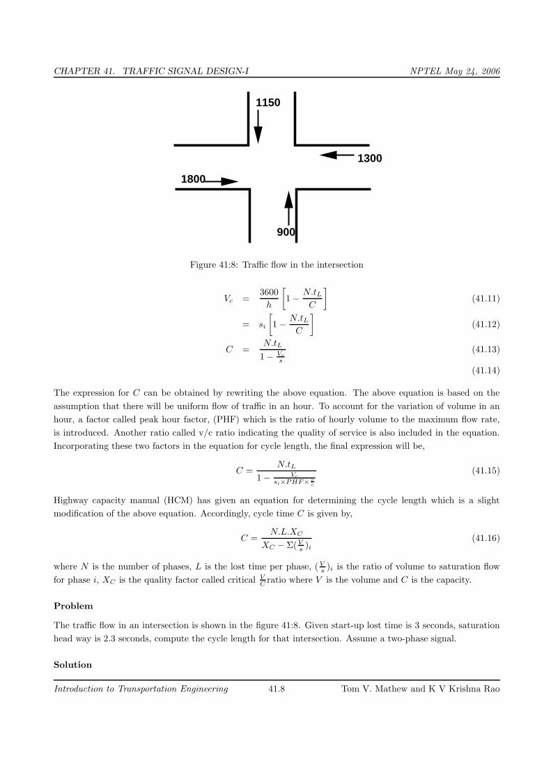
CHAPTER 41. TRAFFIC SIGNAL DESIGN-I NPTEL May 24, 2006
1150
900
1300
1800
Figure 41:8: Traffic flow in the intersection
Vc =3600
h
[
1 −N.tL
C
]
(41.11)
= si
[
1 −N.tL
C
]
(41.12)
C =N.tL
1 − Vc
s
(41.13)
(41.14)
The expression for C can be obtained by rewriting the above equation. The above equation is based on the
assumption that there will be uniform flow of traffic in an hour. To account for the variation of volume in an
hour, a factor called peak hour factor, (PHF) which is the ratio of hourly volume to the maximum flow rate,
is introduced. Another ratio called v/c ratio indicating the quality of service is also included in the equation.
Incorporating these two factors in the equation for cycle length, the final expression will be,
C =N.tL
1 − Vc
si×PHF×
v
c
(41.15)
Highway capacity manual (HCM) has given an equation for determining the cycle length which is a slight
modification of the above equation. Accordingly, cycle time C is given by,
C =N.L.XC
XC − Σ(V
s)i
(41.16)
where N is the number of phases, L is the lost time per phase, (V
s)i is the ratio of volume to saturation flow
for phase i, XC is the quality factor called critical V
Cratio where V is the volume and C is the capacity.
Problem
The traffic flow in an intersection is shown in the figure 41:8. Given start-up lost time is 3 seconds, saturation
head way is 2.3 seconds, compute the cycle length for that intersection. Assume a two-phase signal.
Solution
Introduction to Transportation Engineering 41.8 Tom V. Mathew and K V Krishna Rao
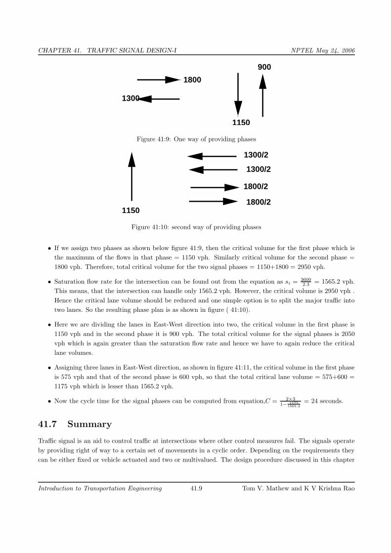
CHAPTER 41. TRAFFIC SIGNAL DESIGN-I NPTEL May 24, 2006
1150
900
1800
1300
Figure 41:9: One way of providing phases
1150
1300/2
1300/2
1800/2
1800/2
Figure 41:10: second way of providing phases
• If we assign two phases as shown below figure 41:9, then the critical volume for the first phase which is
the maximum of the flows in that phase = 1150 vph. Similarly critical volume for the second phase =
1800 vph. Therefore, total critical volume for the two signal phases = 1150+1800 = 2950 vph.
• Saturation flow rate for the intersection can be found out from the equation as si = 3600
2.3= 1565.2 vph.
This means, that the intersection can handle only 1565.2 vph. However, the critical volume is 2950 vph .
Hence the critical lane volume should be reduced and one simple option is to split the major traffic into
two lanes. So the resulting phase plan is as shown in figure ( 41:10).
• Here we are dividing the lanes in East-West direction into two, the critical volume in the first phase is
1150 vph and in the second phase it is 900 vph. The total critical volume for the signal phases is 2050
vph which is again greater than the saturation flow rate and hence we have to again reduce the critical
lane volumes.
• Assigning three lanes in East-West direction, as shown in figure 41:11, the critical volume in the first phase
is 575 vph and that of the second phase is 600 vph, so that the total critical lane volume = 575+600 =
1175 vph which is lesser than 1565.2 vph.
• Now the cycle time for the signal phases can be computed from equation,C = 2×3
1−1175
1565.2
= 24 seconds.
41.7 Summary
Traffic signal is an aid to control traffic at intersections where other control measures fail. The signals operate
by providing right of way to a certain set of movements in a cyclic order. Depending on the requirements they
can be either fixed or vehicle actuated and two or multivalued. The design procedure discussed in this chapter
Introduction to Transportation Engineering 41.9 Tom V. Mathew and K V Krishna Rao
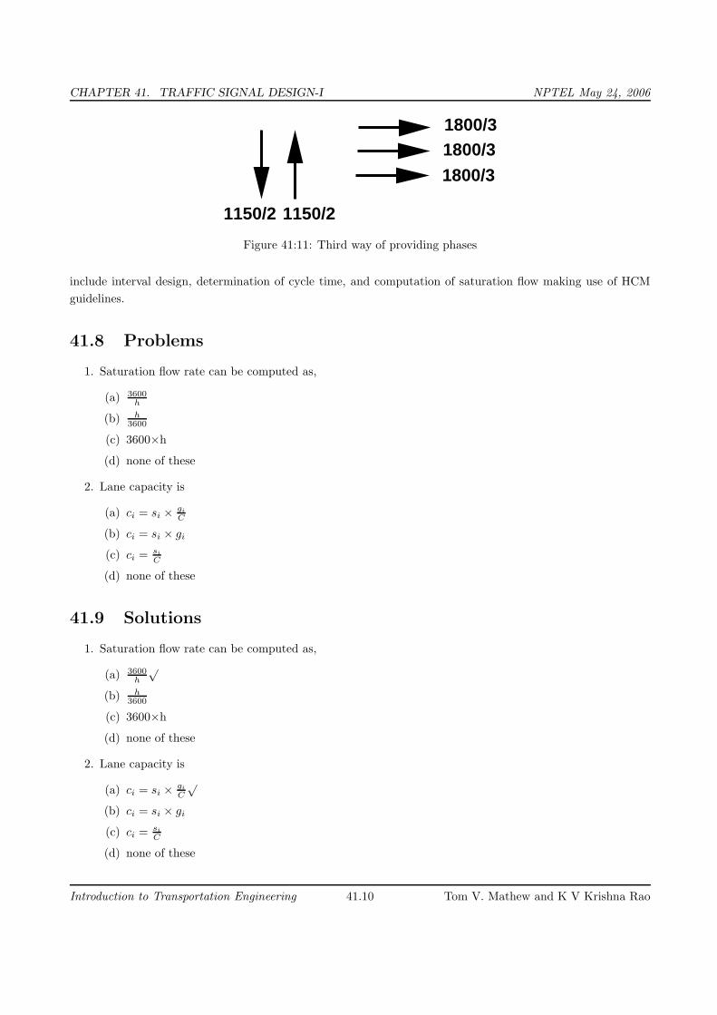
CHAPTER 41. TRAFFIC SIGNAL DESIGN-I NPTEL May 24, 2006
1800/31800/31800/3
1150/2 1150/2
Figure 41:11: Third way of providing phases
include interval design, determination of cycle time, and computation of saturation flow making use of HCM
guidelines.
41.8 Problems
1. Saturation flow rate can be computed as,
(a) 3600
h
(b) h
3600
(c) 3600×h
(d) none of these
2. Lane capacity is
(a) ci = si ×gi
C
(b) ci = si × gi
(c) ci = si
C
(d) none of these
41.9 Solutions
1. Saturation flow rate can be computed as,
(a) 3600
h
√
(b) h
3600
(c) 3600×h
(d) none of these
2. Lane capacity is
(a) ci = si ×gi
C
√
(b) ci = si × gi
(c) ci = si
C
(d) none of these
Introduction to Transportation Engineering 41.10 Tom V. Mathew and K V Krishna Rao
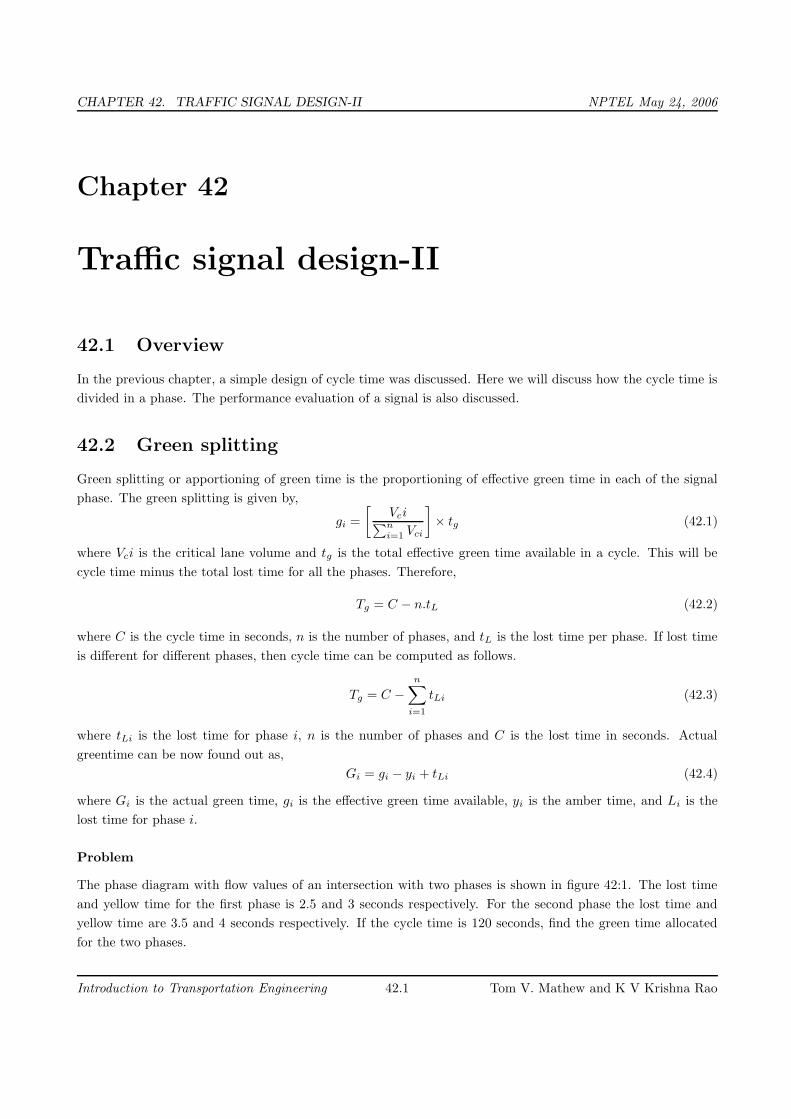
CHAPTER 42. TRAFFIC SIGNAL DESIGN-II NPTEL May 24, 2006
Chapter 42
Traffic signal design-II
42.1 Overview
In the previous chapter, a simple design of cycle time was discussed. Here we will discuss how the cycle time is
divided in a phase. The performance evaluation of a signal is also discussed.
42.2 Green splitting
Green splitting or apportioning of green time is the proportioning of effective green time in each of the signal
phase. The green splitting is given by,
gi =
[
Vci∑
n
i=1Vci
]
× tg (42.1)
where Vci is the critical lane volume and tg is the total effective green time available in a cycle. This will be
cycle time minus the total lost time for all the phases. Therefore,
Tg = C − n.tL (42.2)
where C is the cycle time in seconds, n is the number of phases, and tL is the lost time per phase. If lost time
is different for different phases, then cycle time can be computed as follows.
Tg = C −
n∑
i=1
tLi (42.3)
where tLi is the lost time for phase i, n is the number of phases and C is the lost time in seconds. Actual
greentime can be now found out as,
Gi = gi − yi + tLi (42.4)
where Gi is the actual green time, gi is the effective green time available, yi is the amber time, and Li is the
lost time for phase i.
Problem
The phase diagram with flow values of an intersection with two phases is shown in figure 42:1. The lost time
and yellow time for the first phase is 2.5 and 3 seconds respectively. For the second phase the lost time and
yellow time are 3.5 and 4 seconds respectively. If the cycle time is 120 seconds, find the green time allocated
for the two phases.
Introduction to Transportation Engineering 42.1 Tom V. Mathew and K V Krishna Rao
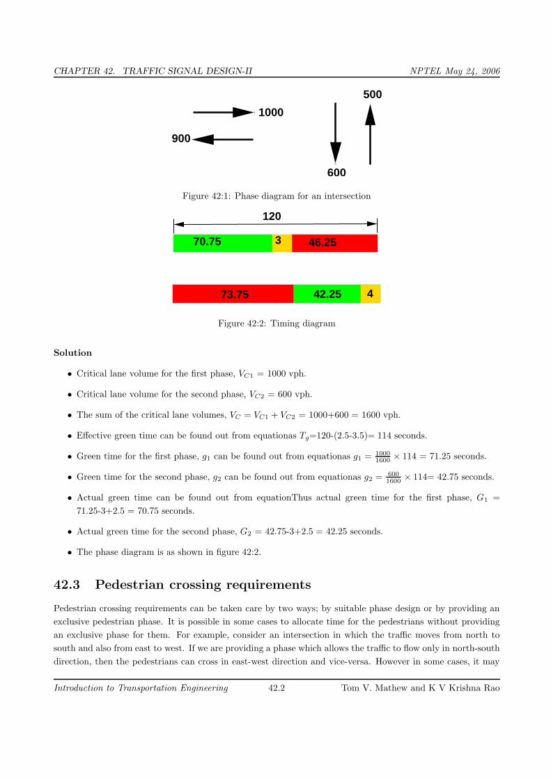
CHAPTER 42. TRAFFIC SIGNAL DESIGN-II NPTEL May 24, 2006
600
500
900
1000
Figure 42:1: Phase diagram for an intersection
�����������������������������������������������������������������������������������������������������������������������������������������������������������������������������������������������������������������������������������������������������
�����������������������������������������������������������������������������������������������������������������������������������������������������������������������������������������������������������������������������������������������������
���������������������������������������������������������������������������������������������������������������������������������������������������������������������������������������������������������������������������������������
�������������������������������������������������������������������������������������������������������������������������������������������������������������������������������������������������������������������������
���������������������������������������������������������������
���������������������������������������������������������������
70.75 3 46.25
������������������������������������������������������������������������������������������������������������������������������������������������������������������������������������������������������
������������������������������������������������������������������������������������������������������������������������������������������������������������������������������������������������������
������������������
������������������
������������������������������������������������������������������������������������������������������������������������������������������������������������������������������������������������������������������������������
������������������������������������������������������������������������������������������������������������������������������������������������������������������������������������������������������������������
� � � � � � � � � � � � � � � � � � � � � � � �
������������������������������������������������������
����������������������������������������������������������������������������������������������������������������������������������������������������������������������������������������������������������������������������������������������������������������������������������������������������
������
73.75 42.25 4
120
Figure 42:2: Timing diagram
Solution
• Critical lane volume for the first phase, VC1 = 1000 vph.
• Critical lane volume for the second phase, VC2 = 600 vph.
• The sum of the critical lane volumes, VC = VC1 + VC2 = 1000+600 = 1600 vph.
• Effective green time can be found out from equationas Tg=120-(2.5-3.5)= 114 seconds.
• Green time for the first phase, g1 can be found out from equationas g1 = 1000
1600× 114 = 71.25 seconds.
• Green time for the second phase, g2 can be found out from equationas g2 = 600
1600× 114= 42.75 seconds.
• Actual green time can be found out from equationThus actual green time for the first phase, G1 =
71.25-3+2.5 = 70.75 seconds.
• Actual green time for the second phase, G2 = 42.75-3+2.5 = 42.25 seconds.
• The phase diagram is as shown in figure 42:2.
42.3 Pedestrian crossing requirements
Pedestrian crossing requirements can be taken care by two ways; by suitable phase design or by providing an
exclusive pedestrian phase. It is possible in some cases to allocate time for the pedestrians without providing
an exclusive phase for them. For example, consider an intersection in which the traffic moves from north to
south and also from east to west. If we are providing a phase which allows the traffic to flow only in north-south
direction, then the pedestrians can cross in east-west direction and vice-versa. However in some cases, it may
Introduction to Transportation Engineering 42.2 Tom V. Mathew and K V Krishna Rao
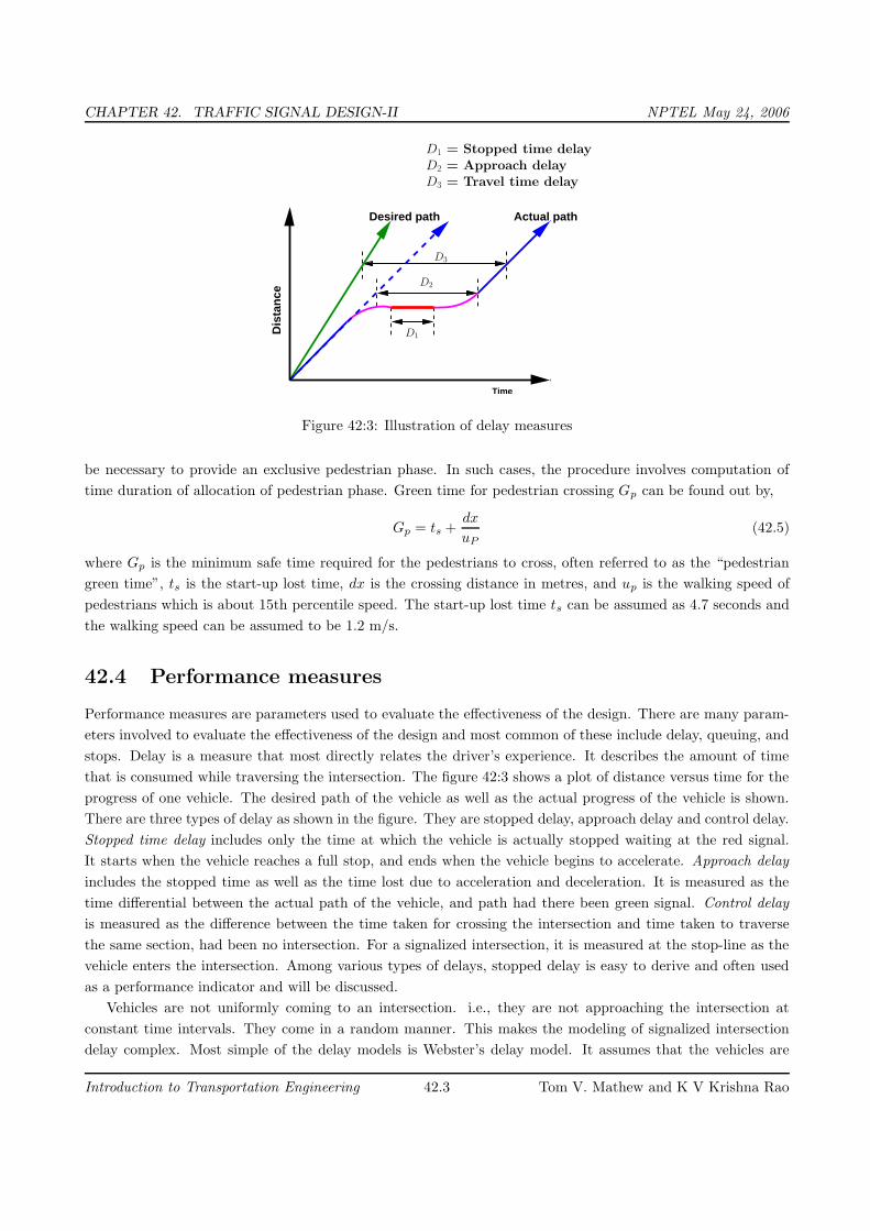
CHAPTER 42. TRAFFIC SIGNAL DESIGN-II NPTEL May 24, 2006
Time
Desired path Actual path
Dis
tan
ce
D3
D2
D1
D3 = Travel time delay
D2 = Approach delay
D1 = Stopped time delay
Figure 42:3: Illustration of delay measures
be necessary to provide an exclusive pedestrian phase. In such cases, the procedure involves computation of
time duration of allocation of pedestrian phase. Green time for pedestrian crossing Gp can be found out by,
Gp = ts +dx
uP
(42.5)
where Gp is the minimum safe time required for the pedestrians to cross, often referred to as the “pedestrian
green time”, ts is the start-up lost time, dx is the crossing distance in metres, and up is the walking speed of
pedestrians which is about 15th percentile speed. The start-up lost time ts can be assumed as 4.7 seconds and
the walking speed can be assumed to be 1.2 m/s.
42.4 Performance measures
Performance measures are parameters used to evaluate the effectiveness of the design. There are many param-
eters involved to evaluate the effectiveness of the design and most common of these include delay, queuing, and
stops. Delay is a measure that most directly relates the driver’s experience. It describes the amount of time
that is consumed while traversing the intersection. The figure 42:3 shows a plot of distance versus time for the
progress of one vehicle. The desired path of the vehicle as well as the actual progress of the vehicle is shown.
There are three types of delay as shown in the figure. They are stopped delay, approach delay and control delay.
Stopped time delay includes only the time at which the vehicle is actually stopped waiting at the red signal.
It starts when the vehicle reaches a full stop, and ends when the vehicle begins to accelerate. Approach delay
includes the stopped time as well as the time lost due to acceleration and deceleration. It is measured as the
time differential between the actual path of the vehicle, and path had there been green signal. Control delay
is measured as the difference between the time taken for crossing the intersection and time taken to traverse
the same section, had been no intersection. For a signalized intersection, it is measured at the stop-line as the
vehicle enters the intersection. Among various types of delays, stopped delay is easy to derive and often used
as a performance indicator and will be discussed.
Vehicles are not uniformly coming to an intersection. i.e., they are not approaching the intersection at
constant time intervals. They come in a random manner. This makes the modeling of signalized intersection
delay complex. Most simple of the delay models is Webster’s delay model. It assumes that the vehicles are
Introduction to Transportation Engineering 42.3 Tom V. Mathew and K V Krishna Rao
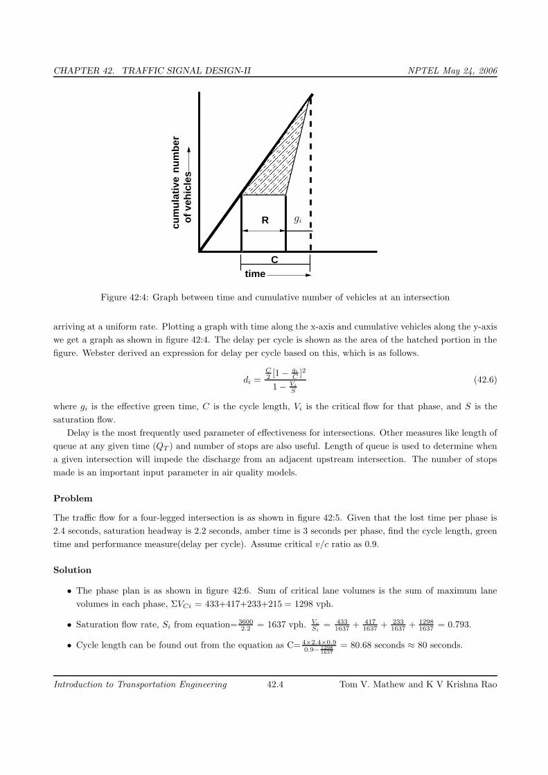
CHAPTER 42. TRAFFIC SIGNAL DESIGN-II NPTEL May 24, 2006
��������������������������������������������������������������������������������������������������������������������������������������������������������������������������������������������������������������������������������������������������������������������������������������������������������������������������������������������������������������������������������
��������������������������������������������������������������������������������������������������������������������������������������������������������������������������������������������������������������������������������������������������������������������������������������������������������������������������������������������������������������������������������
�������
�������
Rcum
ula
tive
nu
mb
ero
fveh
icle
s
Ctime
gi
Figure 42:4: Graph between time and cumulative number of vehicles at an intersection
arriving at a uniform rate. Plotting a graph with time along the x-axis and cumulative vehicles along the y-axis
we get a graph as shown in figure 42:4. The delay per cycle is shown as the area of the hatched portion in the
figure. Webster derived an expression for delay per cycle based on this, which is as follows.
di =C
2[1 −
gi
C]2
1 − Vi
S
(42.6)
where gi is the effective green time, C is the cycle length, Vi is the critical flow for that phase, and S is the
saturation flow.
Delay is the most frequently used parameter of effectiveness for intersections. Other measures like length of
queue at any given time (QT ) and number of stops are also useful. Length of queue is used to determine when
a given intersection will impede the discharge from an adjacent upstream intersection. The number of stops
made is an important input parameter in air quality models.
Problem
The traffic flow for a four-legged intersection is as shown in figure 42:5. Given that the lost time per phase is
2.4 seconds, saturation headway is 2.2 seconds, amber time is 3 seconds per phase, find the cycle length, green
time and performance measure(delay per cycle). Assume critical v/c ratio as 0.9.
Solution
• The phase plan is as shown in figure 42:6. Sum of critical lane volumes is the sum of maximum lane
volumes in each phase, ΣVCi = 433+417+233+215 = 1298 vph.
• Saturation flow rate, Si from equation= 3600
2.2= 1637 vph. Vc
Si
= 433
1637+ 417
1637+ 233
1637+ 1298
1637= 0.793.
• Cycle length can be found out from the equation as C= 4×2.4×0.9
0.9−1298
1637
= 80.68 seconds ≈ 80 seconds.
Introduction to Transportation Engineering 42.4 Tom V. Mathew and K V Krishna Rao
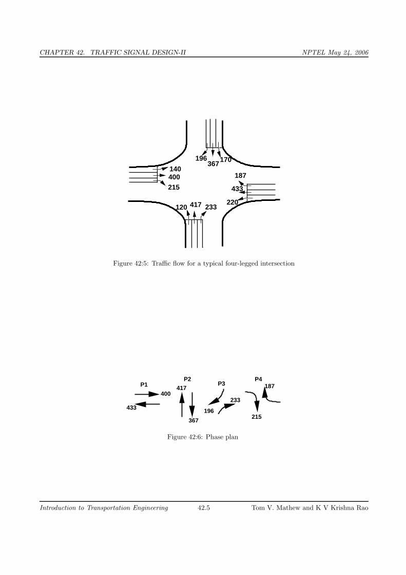
CHAPTER 42. TRAFFIC SIGNAL DESIGN-II NPTEL May 24, 2006
���������
215400140
196367170
187
433
220120 417 233
Figure 42:5: Traffic flow for a typical four-legged intersection
P1
433
400
P2
417
367
P3
196
233
P4
215
187
Figure 42:6: Phase plan
Introduction to Transportation Engineering 42.5 Tom V. Mathew and K V Krishna Rao
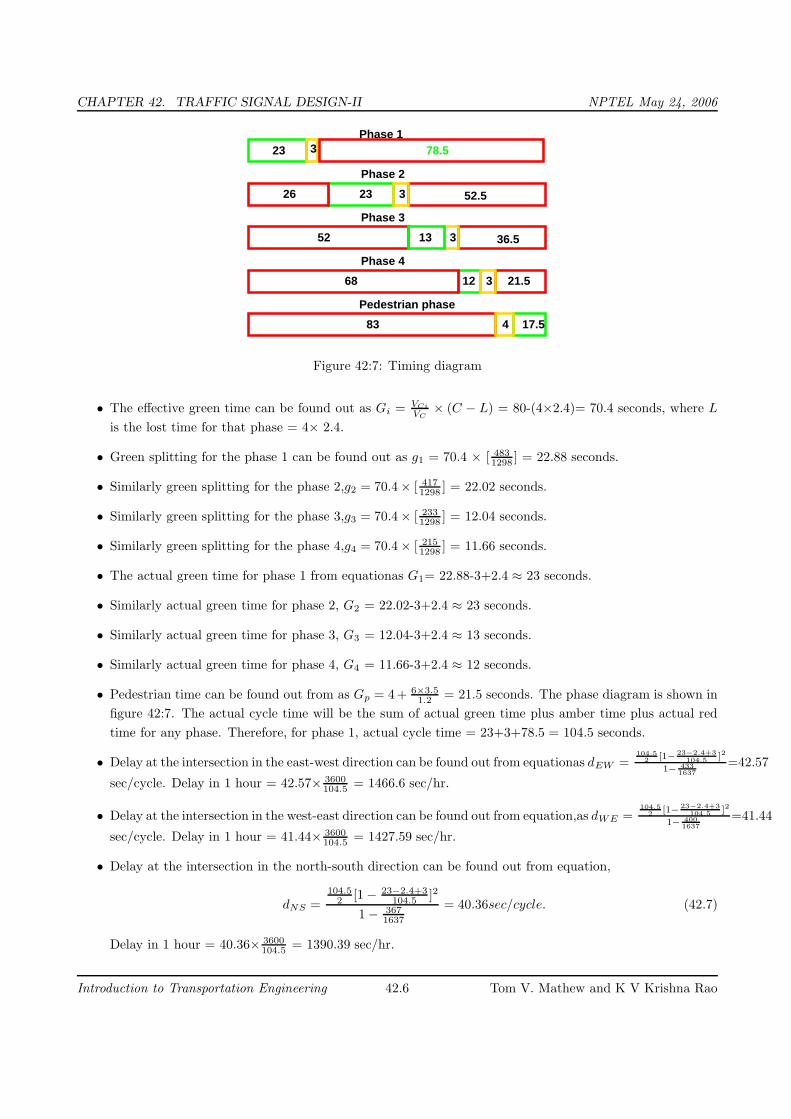
CHAPTER 42. TRAFFIC SIGNAL DESIGN-II NPTEL May 24, 2006
Phase 1
Phase 2
Phase 4
Pedestrian phase
23 3 78.5
26
Phase 3
52
3
4
13
1268
3
23 3
17.583
21.5
36.5
52.5
Figure 42:7: Timing diagram
• The effective green time can be found out as Gi = VCi
VC
× (C − L) = 80-(4×2.4)= 70.4 seconds, where L
is the lost time for that phase = 4× 2.4.
• Green splitting for the phase 1 can be found out as g1 = 70.4 × [ 483
1298] = 22.88 seconds.
• Similarly green splitting for the phase 2,g2 = 70.4× [ 417
1298] = 22.02 seconds.
• Similarly green splitting for the phase 3,g3 = 70.4× [ 233
1298] = 12.04 seconds.
• Similarly green splitting for the phase 4,g4 = 70.4× [ 215
1298] = 11.66 seconds.
• The actual green time for phase 1 from equationas G1= 22.88-3+2.4 ≈ 23 seconds.
• Similarly actual green time for phase 2, G2 = 22.02-3+2.4 ≈ 23 seconds.
• Similarly actual green time for phase 3, G3 = 12.04-3+2.4 ≈ 13 seconds.
• Similarly actual green time for phase 4, G4 = 11.66-3+2.4 ≈ 12 seconds.
• Pedestrian time can be found out from as Gp = 4 + 6×3.5
1.2= 21.5 seconds. The phase diagram is shown in
figure 42:7. The actual cycle time will be the sum of actual green time plus amber time plus actual red
time for any phase. Therefore, for phase 1, actual cycle time = 23+3+78.5 = 104.5 seconds.
• Delay at the intersection in the east-west direction can be found out from equationas dEW =104.5
2[1−
23−2.4+3
104.5]2
1−433
1637
=42.57
sec/cycle. Delay in 1 hour = 42.57× 3600
104.5= 1466.6 sec/hr.
• Delay at the intersection in the west-east direction can be found out from equation,as dWE =104.5
2[1−
23−2.4+3
104.5]2
1−400
1637
=41.44
sec/cycle. Delay in 1 hour = 41.44× 3600
104.5= 1427.59 sec/hr.
• Delay at the intersection in the north-south direction can be found out from equation,
dNS =104.5
2[1 − 23−2.4+3
104.5]2
1 − 367
1637
= 40.36sec/cycle. (42.7)
Delay in 1 hour = 40.36× 3600
104.5= 1390.39 sec/hr.
Introduction to Transportation Engineering 42.6 Tom V. Mathew and K V Krishna Rao
CHAPTER 42. TRAFFIC SIGNAL DESIGN-II NPTEL May 24, 2006
• Delay at the intersection in the south-north direction can be found out from equation,
dSN =104.5
2[1 − 23−2.4+3
104.5]2
1 − 417
1637
= 42.018sec/cycle. (42.8)
Delay in 1 hour = 42.018× 3600
104.5= 1447.51 sec/hr.
• Delay at the intersection in the south-east direction can be found out from equation,
dSE =104.5
2[1 − 13−2.4+3
104.5]2
1 − 233
1637
= 46.096sec/cycle. (42.9)
Delay in 1 hour = 46.096× 3600
104.5= 1587.996 sec/hr.
• Delay at the intersection in the north-west direction can be found out from equation,
dNW =104.5
2[1 − 13−2.4+3
104.5]2
1 − 196
1637
= 44.912sec/cycle. (42.10)
Delay in 1 hour = 44.912× 3600
104.5= 1547.21 sec/hr.
• Delay at the intersection in the west-south direction can be found out from equation,
dWS =104.5
2[1 − 12−2.4+3
104.5]2
1 − 215
1637
= 46.52sec/cycle. (42.11)
Delay in 1 hour = 46.52× 3600
104.5= 1602.60 sec/hr.
• Delay at the intersection in the east-north direction can be found out from equation,
dEN =104.5
2[1 − 12−2.4+3
104.5]2
1 − 187
1637
= 45.62sec/cycle. (42.12)
Delay in 1 hour = 45.62× 3600
104.5= 1571.598 sec/hr.
42.5 Summary
Green splitting is done by proportioning the green time among various phases according to the critical volume
of the phase. Pedestrian phases are provided by considering the walking speed and start-up lost time. Like
other facilities, signals are also assessed for performance, delay being th e important parameter used.
42.6 Problems
1. Table shows the traffic flow for a four-legged intersection. The lost time per phase is 2.4 seconds, saturation
headway is 2.2 seconds, amber time is 3 seconds per phase. Find the cycle length, green time and
performance measure. Assume critical volume to capacity ratio as 0.85. Draw the phasing and timing
diagrams.
From To Flow(veh/hr)
North South 750
East West 650
West East 500
Introduction to Transportation Engineering 42.7 Tom V. Mathew and K V Krishna Rao
CHAPTER 42. TRAFFIC SIGNAL DESIGN-II NPTEL May 24, 2006
P1 P2
750
450
500
650
Figure 42:8: Phase diagram
P1 P2
450
500
650
750/2750/2
Figure 42:9: Phase diagram
Solution
• Given, saturation headway is 2.2 seconds, total lost time per phase (tL) is 2.4 seconds, saturation flow =3600
2.2= 1636.36 veh/hr. Phasing diagram can be assumed as in figure 42:9.
• Cycle time C can be found from equation= 2×2.4×0.85
0.85−750+650
1636.36
as negative.
• Hence the traffic flowing from north to south can be allowed to flow into two lanes.
• Now cycle time can be find out as 2×2.4×0.85
0.85−450+650
1636.36
= 22.95 or 23 seconds.
• The effective green time , tg = C − (N × tL) = 23 − (2 × 2.4) = 18.2 seconds.
• This green time can be split into two phases as, For phase 1, g1 = 450×18.2
1100= 7.45 seconds. For phase
2, g2 = 650×18.2
1100= 10.75 seconds. Now actual green time ,G1 = g1 minus amber time plus lost time.
Therefore, G1 = 7.45-3+2.4 = 6.85 seconds. G2 = 10.75-3+2.4 = 10.15 seconds.
• Timing diagram is as shown in figure 42:10
• Delay at the intersection in the east-west direction can be found out from equationas dEW =23
2[1−
10.75−2.4+3
23]2
1−650
1636.36
=
4.892sec/cycle.
Delay in 1 hour = × 3600
23=765.704 sec/hr.
• Delay at the intersection in the west-east direction can be found out from equation,as dWE =23
2[1−
10.75−2.4+3
23]2
1−500
1636.36
=
4.248sec/cycle.
Delay in 1 hour = × 3600
23=664.90 sec/hr.
Introduction to Transportation Engineering 42.8 Tom V. Mathew and K V Krishna Rao
CHAPTER 42. TRAFFIC SIGNAL DESIGN-II NPTEL May 24, 2006
������������������������������������������������������������������������������������������������������������������������������������������������������������������������������������������������������
������������������������������������������������������������������������������������������������������������������������������������������������������������������������������������������������������
������������������������������������������
������������������������������������������
������������������������������������������������������������������������������������������������������������������������������������������������������������������������������������������������������������������������������
������������������������������������������������������������������������������������������������������������������������������������������������������������������������������������������������������������������
������������������������������������������������������
������������������������������������������������������
������������������������������������������������������������������������������������������������������������������������������������������������
������
�����������������������������������������������������������������������������������������������������������������������������������������������������������������������������������������������������������������������������������������������������
� � � � � � � � � � � � � � � � � � � � � � � � � � � � � � � � � � � � � � � � � � � � � � � � � � � � � � � � � � � � � � � � � � � � � � � � � � � � � � � � � � � � � � � � � � � � � � � � � � � � � � � � � � � � � � � � � � � � � � �
���������������������������������������������������������������������������������������������������������������������������������������������������������������������������������������������������������������������������������������
�������������������������������������������������������������������������������������������������������������������������������������������������������������������������������������������������������������������������
���������������������������������������������������������������
���������������������������������������������������������������
9.85 10.15 3
23
6.85 3 13.15
Phase 2
Phase 1
Figure 42:10: Timing diagram
• Delay at the intersection in the north-south direction can be found out from equation,dNS =23
2[1−
7.45−2.4+3
23]2
1−750
1636.36
=8.97sec/cycle.
Delay in 1 hour = × 3600
23= 1404 sec/hr.
• Delay at the intersection in the south-north direction can be found out from equation,dSN =23
2[1−
7.45−2.4+3
23]2
1−450
1636.36
=6.703sec/cycle.
Delay in 1 hour = × 3600
23=1049.16 sec/hr.
Introduction to Transportation Engineering 42.9 Tom V. Mathew and K V Krishna Rao
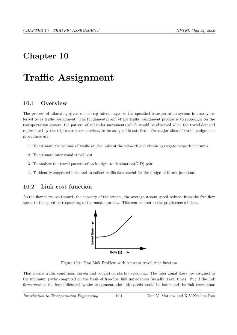
CHAPTER 10. TRAFFIC ASSIGNMENT NPTEL May 24, 2006
Chapter 10
Traffic Assignment
10.1 Overview
The process of allocating given set of trip interchanges to the specified transportation system is usually re-
ferred to as traffic assignment. The fundamental aim of the traffic assignment process is to reproduce on the
transportation system, the pattern of vehicular movements which would be observed when the travel demand
represented by the trip matrix, or matrices, to be assigned is satisfied. The major aims of traffic assignment
procedures are:
1. To estimate the volume of traffic on the links of the network and obtain aggregate network measures.
2. To estimate inter zonal travel cost.
3. To analyze the travel pattern of each origin to destination(O-D) pair.
4. To identify congested links and to collect traffic data useful for the design of future junctions.
10.2 Link cost function
As the flow increases towards the capacity of the stream, the average stream speed reduces from the free flow
speed to the speed corresponding to the maximum flow. This can be seen in the graph shown below.
flow (x)
trav
el t
ime
Figure 10:1: Two Link Problem with constant travel time function
That means traffic conditions worsen and congestion starts developing. The inter zonal flows are assigned to
the minimum paths computed on the basis of free-flow link impedances (usually travel time). But if the link
flows were at the levels dictated by the assignment, the link speeds would be lower and the link travel time
Introduction to Transportation Engineering 10.1 Tom V. Mathew and K V Krishna Rao
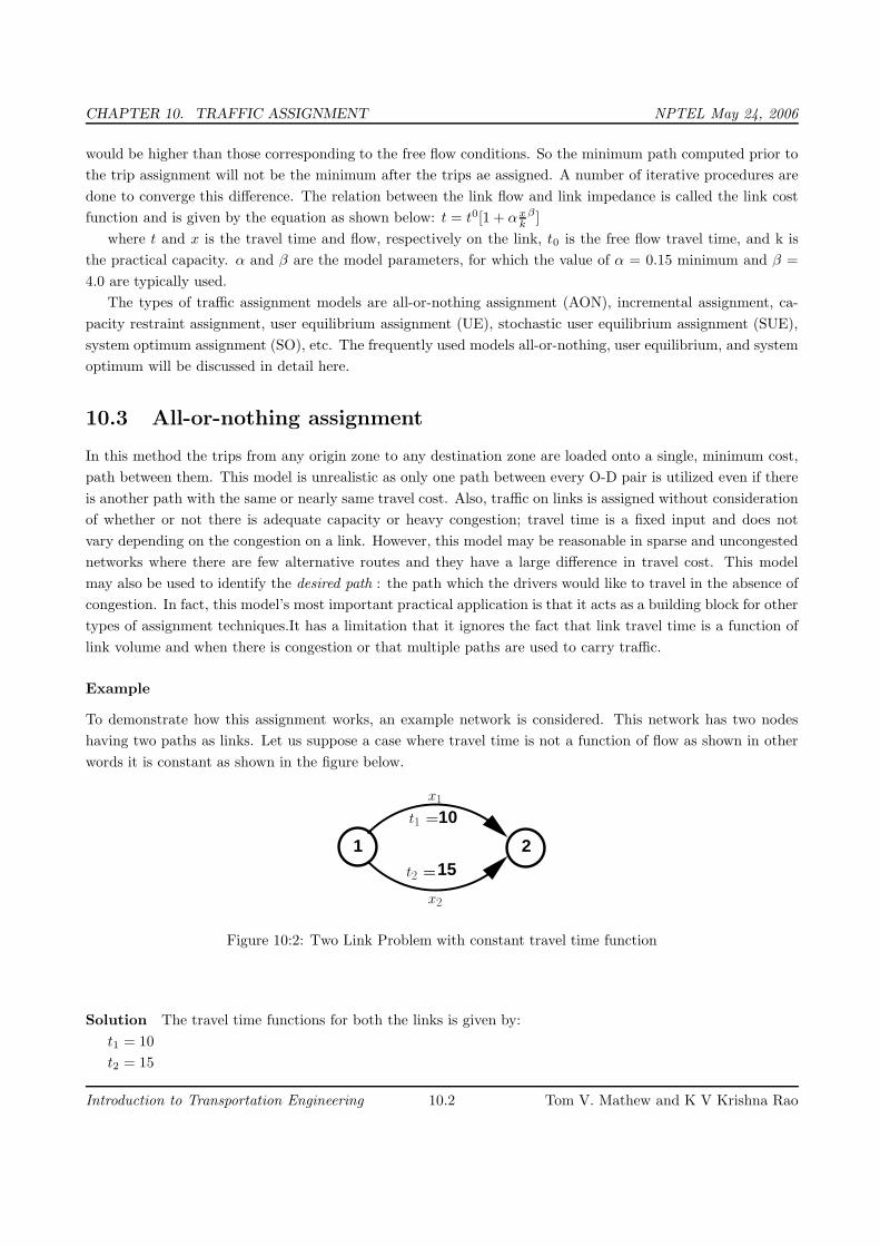
CHAPTER 10. TRAFFIC ASSIGNMENT NPTEL May 24, 2006
would be higher than those corresponding to the free flow conditions. So the minimum path computed prior to
the trip assignment will not be the minimum after the trips ae assigned. A number of iterative procedures are
done to converge this difference. The relation between the link flow and link impedance is called the link cost
function and is given by the equation as shown below: t = t0[1 + αx
k
β ]
where t and x is the travel time and flow, respectively on the link, t0 is the free flow travel time, and k is
the practical capacity. α and β are the model parameters, for which the value of α = 0.15 minimum and β =
4.0 are typically used.
The types of traffic assignment models are all-or-nothing assignment (AON), incremental assignment, ca-
pacity restraint assignment, user equilibrium assignment (UE), stochastic user equilibrium assignment (SUE),
system optimum assignment (SO), etc. The frequently used models all-or-nothing, user equilibrium, and system
optimum will be discussed in detail here.
10.3 All-or-nothing assignment
In this method the trips from any origin zone to any destination zone are loaded onto a single, minimum cost,
path between them. This model is unrealistic as only one path between every O-D pair is utilized even if there
is another path with the same or nearly same travel cost. Also, traffic on links is assigned without consideration
of whether or not there is adequate capacity or heavy congestion; travel time is a fixed input and does not
vary depending on the congestion on a link. However, this model may be reasonable in sparse and uncongested
networks where there are few alternative routes and they have a large difference in travel cost. This model
may also be used to identify the desired path : the path which the drivers would like to travel in the absence of
congestion. In fact, this model’s most important practical application is that it acts as a building block for other
types of assignment techniques.It has a limitation that it ignores the fact that link travel time is a function of
link volume and when there is congestion or that multiple paths are used to carry traffic.
Example
To demonstrate how this assignment works, an example network is considered. This network has two nodes
having two paths as links. Let us suppose a case where travel time is not a function of flow as shown in other
words it is constant as shown in the figure below.
151 2
10
x2
t2 =
x1
t1 =
Figure 10:2: Two Link Problem with constant travel time function
Solution The travel time functions for both the links is given by:
t1 = 10
t2 = 15
Introduction to Transportation Engineering 10.2 Tom V. Mathew and K V Krishna Rao
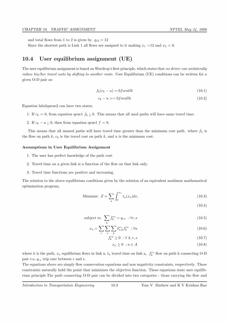
CHAPTER 10. TRAFFIC ASSIGNMENT NPTEL May 24, 2006
and total flows from 1 to 2 is given by. q12 = 12
Since the shortest path is Link 1 all flows are assigned to it making x1 =12 and x2 = 0.
10.4 User equilibrium assignment (UE)
The user equilibrium assignment is based on Wardrop’s first principle, which states that no driver can unilaterally
reduce his/her travel costs by shifting to another route. User Equilibrium (UE) conditions can be written for a
given O-D pair as:
fk(ck − u) = 0forallk (10.1)
ck − u >= 0forallk (10.2)
Equation labelqueue2 can have two states.
1. If ck = 0, from equation qeue1 fk ¿ 0. This means that all used paths will have same travel time.
2. If ck − u ¿ 0, then from equation qeue1 f = 0.
This means that all unused paths will have travel time greater than the minimum cost path. where fk is
the flow on path k, ck is the travel cost on path k, and u is the minimum cost.
Assumptions in User Equilibrium Assignment
1. The user has perfect knowledge of the path cost.
2. Travel time on a given link is a function of the flow on that link only.
3. Travel time functions are positive and increasing.
The solution to the above equilibrium conditions given by the solution of an equivalent nonlinear mathematical
optimization program,
Minimize Z =∑
a
∫
xa
0
ta(xa)dx, (10.3)
(10.4)
subject to∑
k
frs
k= qrs : ∀r, s (10.5)
xa =∑
r
∑
s
∑
k
δrs
a,kfrs
k : ∀a (10.6)
frs
k ≥ 0 : ∀ k, r, s (10.7)
xa ≥ 0 : a ∈ A (10.8)
where k is the path, xa equilibrium flows in link a, ta travel time on link a, f rs
kflow on path k connecting O-D
pair r-s, qrs trip rate between r and s.
The equations above are simply flow conservation equations and non negativity constraints, respectively. These
constraints naturally hold the point that minimizes the objective function. These equations state user equilib-
rium principle.The path connecting O-D pair can be divided into two categories : those carrying the flow and
Introduction to Transportation Engineering 10.3 Tom V. Mathew and K V Krishna Rao
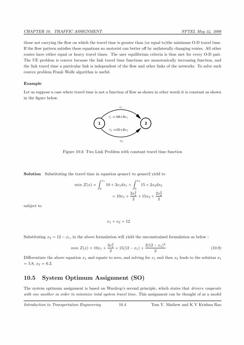
CHAPTER 10. TRAFFIC ASSIGNMENT NPTEL May 24, 2006
those not carrying the flow on which the travel time is greater than (or equal to)the minimum O-D travel time.
If the flow pattern satisfies these equations no motorist can better off by unilaterally changing routes. All other
routes have either equal or heavy travel times. The user equilibrium criteria is thus met for every O-D pair.
The UE problem is convex because the link travel time functions are monotonically increasing function, and
the link travel time a particular link is independent of the flow and other links of the networks. To solve such
convex problem Frank Wolfe algorithm is useful.
Example
Let us suppose a case where travel time is not a function of flow as shown in other words it is constant as shown
in the figure below.
1 2
x1
10+3x1t1 =
t2 =15+2x2
x2
Figure 10:3: Two Link Problem with constant travel time function
Solution Substituting the travel time in equation qeuser1 to qeuser2 yield to
min Z(x) =
∫ x1
0
10 + 3x1dx1 +
∫ x2
0
15 + 2x2dx2
= 10x1 +3x2
1
2+ 15x2 +
2x2
2
2
subject to
x1 + x2 = 12
Substituting x2 = 12− x1, in the above formulation will yield the unconstrained formulation as below :
min Z(x) = 10x1 +3x2
1
2+ 15(12− x1) +
2(12− x1)2
2(10.9)
Differentiate the above equation x1 and equate to zero, and solving for x1 and then x2 leads to the solution x1
= 5.8, x2 = 6.2.
10.5 System Optimum Assignment (SO)
The system optimum assignment is based on Wardrop’s second principle, which states that drivers cooperate
with one another in order to minimize total system travel time. This assignment can be thought of as a model
Introduction to Transportation Engineering 10.4 Tom V. Mathew and K V Krishna Rao
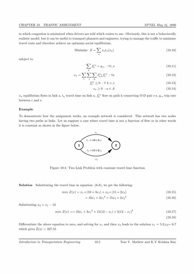
CHAPTER 10. TRAFFIC ASSIGNMENT NPTEL May 24, 2006
in which congestion is minimized when drivers are told which routes to use. Obviously, this is not a behaviorally
realistic model, but it can be useful to transport planners and engineers, trying to manage the traffic to minimize
travel costs and therefore achieve an optimum social equilibrium.
Minimize Z =∑
a
xata(xa) (10.10)
subject to∑
k
frs
k = qrs : ∀r, s (10.11)
xa =∑
r
∑
s
∑
k
δrs
a,kfrs
k: ∀a (10.12)
frs
k≥ 0 : ∀ k, r, s (10.13)
xa ≥ 0 : a ∈ A (10.14)
xa equilibrium flows in link a, ta travel time on link a, f rs
kflow on path k connecting O-D pair r-s, qrs trip rate
between r and s.
Example
To demonstrate how the assignment works, an example network is considered. This network has two nodes
having two paths as links. Let us suppose a case where travel time is not a function of flow or in other words
it is constant as shown in the figure below.
1 2
x1
10+3x1t1 =
t2 =15+2x2
x2
Figure 10:4: Two Link Problem with constant travel time function
Solution Substituting the travel time in equation: (6-8), we get the following:
min Z(x) = x1 ∗ (10 + 3x1) + x2 ∗ (15 + 2x2) (10.15)
= 10x1 + 3x12 + 15x2 + 2x2
2 (10.16)
Substituting x2 = x1 − 12
min Z(x) == 10x1 + 3x12 + 15(12− x1) + 2(12− x1)
2(10.17)
(10.18)
Differentiate the above equation to zero, and solving for x1 and then x2 leads to the solution x1 = 5.3,x2= 6.7
which gives Z(x) = 327.55
Introduction to Transportation Engineering 10.5 Tom V. Mathew and K V Krishna Rao
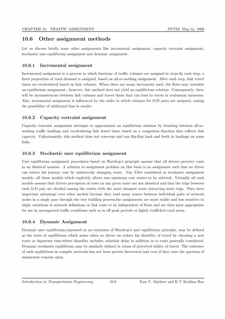
CHAPTER 10. TRAFFIC ASSIGNMENT NPTEL May 24, 2006
10.6 Other assignment methods
Let us discuss briefly some other assignments like incremental assignment, capacity restraint assignment,
stochastic user equilibrium assignment and dynamic assignment.
10.6.1 Incremental assignment
Incremental assignment is a process in which fractions of traffic volumes are assigned in steps.In each step, a
fixed proportion of total demand is assigned, based on all-or-nothing assignment. After each step, link travel
times are recalculated based on link volumes. When there are many increments used, the flows may resemble
an equilibrium assignment ; however, this method does not yield an equilibrium solution. Consequently, there
will be inconsistencies between link volumes and travel times that can lead to errors in evaluation measures.
Also, incremental assignment is influenced by the order in which volumes for O-D pairs are assigned, raising
the possibility of additional bias in results.
10.6.2 Capacity restraint assignment
Capacity restraint assignment attempts to approximate an equilibrium solution by iterating between all-or-
nothing traffic loadings and recalculating link travel times based on a congestion function that reflects link
capacity. Unfortunately, this method does not converge and can flip-flop back and forth in loadings on some
links.
10.6.3 Stochastic user equilibrium assignment
User equilibrium assignment procedures based on Wardrop’s principle assume that all drivers perceive costs
in an identical manner. A solution to assignment problem on this basis is an assignment such that no driver
can reduce his journey cost by unilaterally changing route. Van Vilet considered as stochastic assignment
models, all those models which explicitly allows non minimum cost routes to be selected. Virtually all such
models assume that drivers perception of costs on any given route are not identical and that the trips between
each O-D pair are divided among the routes with the most cheapest route attracting most trips. They have
important advantage over other models because they load many routes between individual pairs of network
nodes in a single pass through the tree building process,the assignments are more stable and less sensitive to
slight variations in network definitions or link costs to be independent of flows and are thus most appropriate
for use in uncongested traffic conditions such as in off peak periods or lightly trafficked rural areas.
10.6.4 Dynamic Assignment
Dynamic user equilibrium,expressed as an extension of Wardrop’s user equilibrium principle, may be defined
as the state of equilibrium which arises when no driver an reduce his disutility of travel by choosing a new
route or departure time,where disutility includes, schedule delay in addition in to costs generally considered.
Dynamic stochastic equilibrium may be similarly defined in terms of perceived utility of travel. The existence
of such equilibrium in complex networks has not been proven theoretical and even if they exist the question of
uniqueness remains open.
Introduction to Transportation Engineering 10.6 Tom V. Mathew and K V Krishna Rao
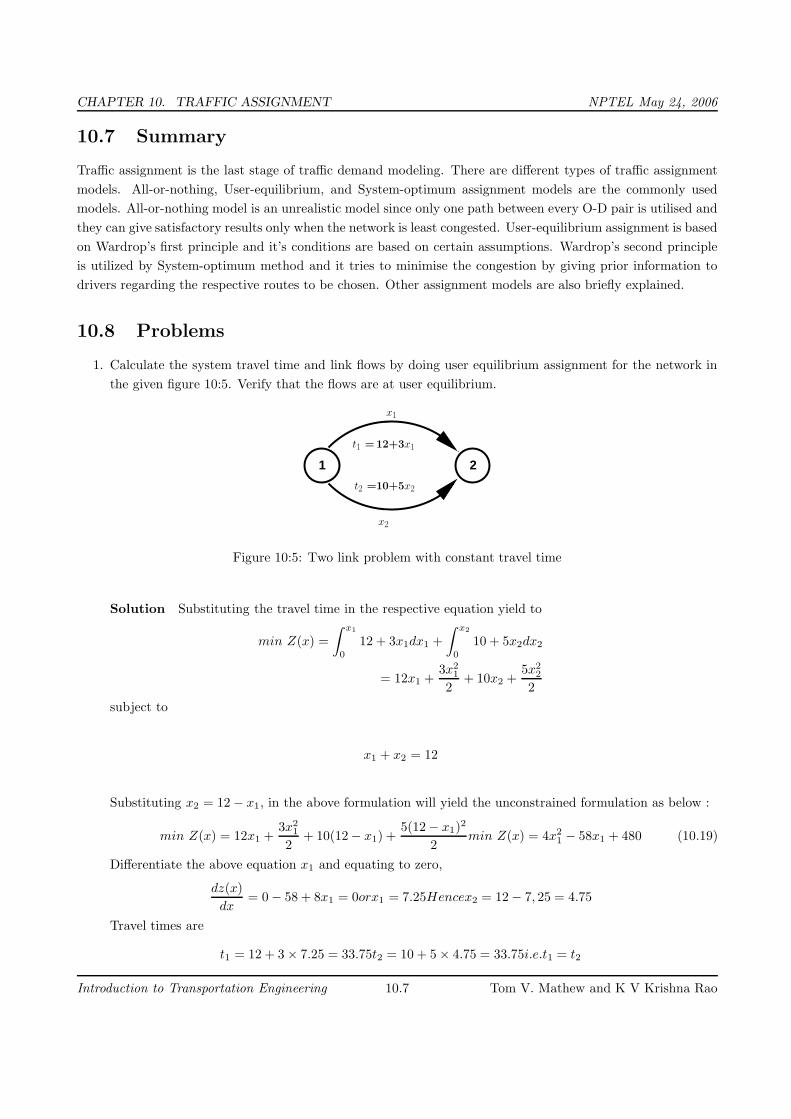
CHAPTER 10. TRAFFIC ASSIGNMENT NPTEL May 24, 2006
10.7 Summary
Traffic assignment is the last stage of traffic demand modeling. There are different types of traffic assignment
models. All-or-nothing, User-equilibrium, and System-optimum assignment models are the commonly used
models. All-or-nothing model is an unrealistic model since only one path between every O-D pair is utilised and
they can give satisfactory results only when the network is least congested. User-equilibrium assignment is based
on Wardrop’s first principle and it’s conditions are based on certain assumptions. Wardrop’s second principle
is utilized by System-optimum method and it tries to minimise the congestion by giving prior information to
drivers regarding the respective routes to be chosen. Other assignment models are also briefly explained.
10.8 Problems
1. Calculate the system travel time and link flows by doing user equilibrium assignment for the network in
the given figure 10:5. Verify that the flows are at user equilibrium.
1 2
12+3x1
t2 =10+5x2
x1
x2
t1 =
Figure 10:5: Two link problem with constant travel time
Solution Substituting the travel time in the respective equation yield to
min Z(x) =
∫
x1
0
12 + 3x1dx1 +
∫
x2
0
10 + 5x2dx2
= 12x1 +3x2
1
2+ 10x2 +
5x2
2
2
subject to
x1 + x2 = 12
Substituting x2 = 12 − x1, in the above formulation will yield the unconstrained formulation as below :
min Z(x) = 12x1 +3x2
1
2+ 10(12− x1) +
5(12− x1)2
2min Z(x) = 4x2
1− 58x1 + 480 (10.19)
Differentiate the above equation x1 and equating to zero,
dz(x)
dx= 0 − 58 + 8x1 = 0orx1 = 7.25Hencex2 = 12− 7, 25 = 4.75
Travel times are
t1 = 12 + 3 × 7.25 = 33.75t2 = 10 + 5 × 4.75 = 33.75i.e.t1 = t2
Introduction to Transportation Engineering 10.7 Tom V. Mathew and K V Krishna Rao

CHAPTER 10. TRAFFIC ASSIGNMENT NPTEL May 24, 2006
It follows that the travel times are at user equilibrium.
Introduction to Transportation Engineering 10.8 Tom V. Mathew and K V Krishna Rao