Traffic engineering of MPLS backbone networks in the presence of heterogeneous streams

Computer Networks 53 (2009) 2688–2702

Contents lists available at ScienceDirect

Computer Networks

journal homepage: www.elsevier .com/locate /comnet

Traffic engineering of MPLS backbone networks in the presenceof heterogeneous streams

Shekhar Srivastava 1, Appie van de Liefvoort, Deep Medhi *

Computer Science and Electrical Engineering Department, University of Missouri–Kansas City, Kansas City, MO 64110, United States

a r t i c l e i n f o

Article history:Received 13 January 2008Received in revised form 3 February 2009Accepted 8 June 2009Available online 16 June 2009

Responsible Editor: G. Ventre

Keywords:MPLSTraffic engineeringTunneling constraintTraffic distortionQuadratic/linear integer programmingDecomposition algorithm

1389-1286/$ - see front matter � 2009 Elsevier B.Vdoi:10.1016/j.comnet.2009.06.003

* Corresponding author. Tel.: +1 816 235 2006; faE-mail address: [email protected] (D. Medhi).

1 Present address: Huawei Technologies, Plano, TX

a b s t r a c t

Heterogeneous streams (due to issues such as disparate traffic characteristics of eachstream, or competing customers’ traffic) raise the issue of whether to multiplex (someof) these streams. In an MPLS network, such multiplexing can be considered by putting dif-ferent streams into a tunnel identified by a single label-switched path (LSP), assuming thatthe different LSPs are assigned a reserved share of the resources. This issue becomes evenmore important in the traffic engineering of a backbone network when a decision needs tobe made on which streams to multiplex when there are constraints on tunneling andcapacity along with routing requirements for tunnels. In this paper, we introduce a distor-tion factor due to heterogeneous streams in traffic engineering of MPLS backbone networksin the presence of tunneling and capacity constraints by formulating a distortion-awarenon-linear discrete optimization problem. Furthermore, we present a two-phase heuristicapproach to solve this formulation efficiently. In the first phase, the problem is decoupledinto two subproblems and in the second phase we show how the non-linear problem (forone of the subproblems) can be simplified. We then present numerical results for bothsmall and large networks to show where and how our approach helps to determine whenand which streams to multiplex depending on whether the tunneling and/or capacity con-straint is dominant; furthermore, by comparing our distortion-aware traffic engineeringmodel with a distortion-ignorant traffic engineering model, we show the benefits of ourapproach.

� 2009 Elsevier B.V. All rights reserved.

1. Introduction

Traffic, at the packet level for different applications,tends to have different characteristics. This fact has beenobserved for emerging applications such as video confer-encing, peer-to-peer, and multimedia applications [1,4].Moreover, heterogeneous traffic streams are multiplexedtogether to share the same link. When traffic of differentcharacteristics are multiplexed together, traffic distortionoccurs which can be significant depending on the charac-teristics of the streams [9,18]. Specifically, such impactscan be fairly strong when one or more of them are

. All rights reserved.

x: +1 816 235 5159.

, United States.

correlated in nature. Besides distortion due to disparatetraffic characteristics, a provider might have preferencenot to combine certain streams because they belong totraffics of competing customers and thus, may want to im-pose an induced distortion for the purpose of trafficengineering.

Consider now an MPLS (multi-protocol label switching)network with label-switched paths, potentially for differ-ent heterogeneous streams (for ease of discussion, label-switched paths and tunnels will be used interchangeably).We define tunnel as the unit of flow to which a certainbandwidth is allocated at each router that it traverses. Ifmultiple paths are being aggregated to share bandwidth,then all of such paths together would be considered atunnel. In order to minimize distortion, a possibleapproach would be to classify and multiplex appropriate

http://dx.doi.org/10.1016/j.comnet.2009.06.003

mailto:[email protected]

http://www.sciencedirect.com/science/journal/13891286

http://www.elsevier.com/locate/comnet

S. Srivastava et al. / Computer Networks 53 (2009) 2688–2702 2689

streams into tunnels so that distortion is minimized withina tunnel. That is, ‘‘like-minded” streams can avoid (or min-imize) distortion if the network has the capability to do so.For this purpose, one can consider the MPLS network inwhich multiple label-switched path (LSP) tunnels can beset up between source and destination nodes; such tunnelscan be used to ensure logical separation between streamsin order to minimize distortions. Therefore, we require thatthe LSPs are setup with a proper amount of allocated band-width and that the routers enforce bandwidth separationamong the LSPs.

There are a number of ways to decide how to takeadvantage of the tunneling idea. On one extreme, a sepa-rate tunnel for each possible traffic stream can be set upto avoid any distortion. The difficulty with this approachis that the number of tunnels can be prohibitively large.This then impacts packet processing and forwarding atan MPLS router [22] and furthermore, administratively,too many tunnels lead to higher network managementcosts. On the other extreme, all streams for the samesource–destination node pairs can be multiplexed in thesame tunnel. Such an allocation will result in streams hav-ing a considerably high amount of distortion, while admin-istrative overhead on managing tunnels and lookup costcan be minimized.

1.1. Contributions of the paper

In this work, we address the trade-off between distor-tion and manageability of label-switched paths in an MPLSnetwork, The scope of our work resides in short- to med-ium-term traffic engineering planning where a networkengineer needs to play with ‘what-if’ scenarios with newlyanticipated demands and customers and what to mixwhile ensuring that the network has enough resources.manageability of label-switched paths in an MPLS net-work. Specifically, we address the following question: gi-ven information on the characteristics of individualstreams and the number of tunnels (LSPs) that can be sup-ported on each link (for example, to avoid impact on thelookup time), can we engineer a network so that the distor-tion level and the required number of tunnels are both ad-dressed together?

In this paper, using a distortion measure [15] (see theAppendix for a brief summary), we construct an optimiza-tion formulation, which minimizes the distortion sufferedby individual streams for different source–destinationnode pairs in a network environment. In addition to thecapacity on a link, the formulation also incorporatesrestrictions in terms of the maximum number of allowedtunnels for manageability. The formulation is general inthe sense that it is transparent to the method used topre-compute the value of the distortion measure; rather,the distortion measure could be induced when consideringcompeting customers. The formulation is a non-linear(quadratic) integer programming problem in nature andhas a large number of binary variables and constraints.To solve this formulation, we propose a two-phase ap-proach in which the first phase is solved by relaxing thebinary variables and the second phase (non-linear objec-tive function) is first linearized and solved using Lagrang-

ian relaxation and subradient optimization. Throughcomputational results, we demonstrate the convergenceof our approach.

Furthermore, we propose several distortion metrics tomeasure distortion at the network-wide and the stream le-vel due to flow interactions. Through numerical results onthese measures, we demonstrate the utility of our formula-tion (‘‘Distortion-Aware Model”) towards allocatingstreams to tunnels while minimizing the distortion suf-fered by the individual streams, compared to the casewhen distortion is not explicitly incorporated (‘‘Distor-tion-Ignorant Model”).

1.2. Related work

Network traffic engineering literature is rich; for exam-ple, see the recent book [14] and the references therein. Inparticular, there have been several works on MPLS trafficengineering [2,7,21]. At the same time, there is little workthat accounts for distortions in a traffic engineering frame-work. The work that is perhaps closest to our work is [20],which studied the problem of routing streams to differentvirtual paths (VPs), i.e., tunnels. This work addressedwhether heterogeneous traffic with different quality-of-service requirements should be segregated on distinct tun-nels or aggregated. They claimed that, in some cases, it isadvantageous, but not always; they developed a criterionon how to make this decision for Gaussian models. Theyfurther commented that it is important to consider hetero-geneous statistical multiplexing or traffic mixes in makingrouting decisions and suggested that multiservice net-works may operate like multiple logical networks, whichare segregated by service type. We, however, take a differ-ent view point. First, we address that it is important to con-sider tunneling restrictions. Second, we consider anetwork-wide approach and also determine the routing/bandwidth allocation of tunnels for heterogeneous trafficstreams through distortion while honoring the capacityand tunneling restrictions. Recently, the notion of limitingtunnels in a traffic engineering formulation for manage-ability has been addressed in a traffic engineering frame-work [16,17]. The issue of tunnels’ growth has recentlyreceived the attention from IETF [22]. To our knowledge,the distortion factor had not been considered before withthe tunneling and capacity requirement in a traffic engi-neering framework.

The formulated traffic engineering problem is a qua-dratic integer programming problem. While there are solu-tion approaches available to solve such problems [8,13],we take advantage of the special structure of the objectivefunction and the constraints to arrive at a simplified solu-tion approach. We draw upon a decoupling heuristic pro-posed in [12] to decouple the main problem; however,our decoupled subproblems are not related to [12] andare solved exploiting the special structure.

1.3. Organization of the paper

The rest of the paper is organized as follows: In Section2, we present the traffic engineering formulation as a qua-dratic integer programming problem. In Section 3, we

q

s

p

Fig. 2. Allocation of streams p; q, and s.

Table 1Notations used in traffic engineering formulation.

N Set of nodes in the networkK Set of demand pairs generating traffic in the networkL Set of links in the networkQk Set of streams for demand pair k 2K

2690 S. Srivastava et al. / Computer Networks 53 (2009) 2688–2702

present our solution approach, which decouples anddecomposes the problem into smaller subproblems. In Sec-tion 4, we present and discuss numerical results, especiallythe benefit of distortion-aware models compared to distor-tion-ignorant models.

2. Traffic engineering modeling

2.1. Distortion

We start with our definition of distortion as it will beused for the purpose of traffic engineering modeling.

Definition 1. Distortion measure Kpq is defined betweentwo streams p and q, where p – q as Kpq P 0, and capturesthe perceived negative impact of the streams on eachother.

This means that Kpq is defined loosely as the extent ofnegative impact in the traffic streams p and q if they aremultiplexed together. Suppose that we are required toroute three streams p; q, and s with the same source anddestination nodes, and we know the pair-wise relationamong streams as Kpq < Kps < Kqs. Suppose then that weonly have two tunnels to route the packets from trafficstreams p; q, and s. Since Kqs is the largest of them (i.e., qand s have the largest distortion), we want to route q ands on different tunnels as shown in Fig. 1. Next, we wantto decide on which tunnel to route the stream p. Since,Kpq < Kps, we route p together with q as shown in Fig. 2and s is routed by itself on the other tunnel. Such a routingensures minimal impact of distortion in all the streamsp; q, and s. Certainly, if there were no tunneling restric-tions, then each stream would get its own tunnel.

Note that by definition, a network engineer would wantto operate the network at a lower value of Kpq. The charac-terization of distortion measure can be based on many dif-ferent requirements. In the Appendix, we present onepossible approach of constructing the distortion measure.In the presented example, distortion is based on the depar-ture distribution of the streams upon leaving the network,and it increases as the extent of corruption with regard to aPoisson source is increased. To see another application,consider a service provider supporting multiple customerson a common integrated MPLS/IP network. Some of thesecustomers could be competitors of each other and hencewould object to sharing a tunnel with each other, whileothers, such as banks providing financial services, wouldnot like to share the traffic with anyone else. In general,for increasing the degree of separation, some might be

q

s

Fig. 1. Allocation of streams q and s only.

willing to pay extra charges while others may be willingto accept sharing to some extent but prefer separation.Developing such a distortion index would require closelyunderstanding the relationships between the customersand the services that they are providing. Such an applica-tion, however interesting, is outside the scope of thispaper.

2.2. Formulation

We now consider a network where heterogenousstreams arriving at a source for a specific destination needto be sent over one of the active tunnels (label-switchedpaths) between the source and the destination (see Table1 for notations) with a goal to minimize distortion. Eachsource–destination pair maintains its own set of tunnels.

The following parameters are assumed to be given:N; K; L; C‘; T‘; Qk, and fk. For every stream p 2 Qk,we assume that average arrival rate kp

k for stream p for pairk is available, and the distortion measure Kpq

km betweenstreams p and q on path m for pair k is pre-computed(see the Appendix) or is available through other mecha-nisms for consideration in the traffic engineeringformulation.

We also assume that a path generator (such as thek-shortest path algorithm) is used to generate the set ofpossible paths, Pk, which will be candidates for tunnels.Let jPkj be the number of candidate paths generated fordemand k 2K. We introduce the decision variable xp

km

associated with the stream p 2 Qk, path m 2 Pk of demandk 2K. Its value is 1 if the traffic of stream p selects path m;

Pk Set of candidates paths for demand pair k 2K

fk Revenue from carrying unit demand volume of demand pairk 2K

kpk Average arrival rate (in Mbps) of stream p 2 Qk; k 2K

Kpqkm Distortion measure between stream p; q 2 Qk on path m 2 Pk

for k 2K

T‘ Maximum number of tunnels allowed on link ‘ 2L

C‘ Capacity of link ‘ 2L (in Mbps)uk; hk Normalization parameters

Variablesxp

km 0/1 decision variable associated with stream p 2 Qk , path m 2 Pk

wkm Tunnel activity (binary) variable associated with pair k 2K,path m 2 Pk


otherwise, its value is 0. Due to capacity restriction, it isquite possible that a demand may not be routed (see Sec-tion 2.3). Considering these aspects, we arrive at the fol-lowing flow constraints:Xm2Pk

xpkm 6 1; p 2 Qk; k 2K; ð1aÞ

xpkm 2 f0;1g; p 2 Qk; m 2 Pk; k 2K: ð1bÞ

To address the flow of the stream of a demand on each link(for each path), we introduce the indicator notation, d, tomap between the demand and the link, as they relate tothe possible paths as follows:

d‘km ¼1 if path m of demand k uses link ‘;

0 otherwise:

�The bandwidth allocated to a tunnel is determined bythe average arrival rate, k (sometimes referred to as thesustained arrival rate), of the streams sharing the tunnel,measured in Mbps. Thus, the bandwidth needed on anylink ‘ (denoted by F‘) to carry flow for different demandscan be captured by the amount:

F‘ ¼Xk2K

Xm2Pk

Xp2Qk

d‘kmkpkxp

km:

For ease of representation, we will henceforth use the tupleðk;m; pÞ to mean k 2K; m 2 Pk; p 2 Qk, along with thecompact summation notation

Pðk;m;pÞ. Since each link ‘

has capacity C‘, the following capacity constraints for eachlink ‘ 2L must be satisfied:Xðk;m;pÞ

d‘kmkpkxp

km 6 C‘; ‘ 2L: ð1cÞ

To incorporate the restriction of limiting the number of ac-tive tunnels on any link ‘ to T‘, we introduce a variable thatcaptures the decision on whether any given path as a tun-nel is being selected or not. The value taken by such a var-iable depends on the value taken by the correspondingflow variables. We define wkm as the tunnel activity vari-able; if it is one, then any of the streams can use the pathand if it is zero, the path is not active and cannot be used.Such a dependency relation can be achieved through thefollowing constraint:

xpkm 6 wkm ðk;m; pÞ: ð1dÞ

Thus, when wkm is 0, constraint (1d) forces xpkm to be 0 for

all p; on the other hand, when wkm is 1, xpkm could be either

0 or 1. The following tunnel constraint limits the number ofactive tunnels on a link:Xðk;mÞ

d‘kmwkm 6 T‘; ‘ 2L; ð1eÞ

wkm 2 f0;1g ðk;mÞ: ð1fÞThus, constraints for the traffic engineering problems areas given from (1a)–(1f). There are, however, multipleobjectives to be considered. One objective is to maximizethe total revenue generated by the flow carried by the net-work while a second objective is to minimize the overallmismatch due to traffic streams sharing tunnels in the net-work. Furthermore, a third objective is to minimize thecost of allocation and maintenance of the tunnels. Weshow below how to construct a composite objective func-

tion based on these three objectives. The first objective, to-tal revenue generated, can be written as:

fr ¼Xðk;m;pÞ

fkkpkxp

km: ð2Þ

Note that we encounter distortions only when for demandk there are any two disparate streams p and q, which sharethe same path m. In other words, only when xp

km ¼ xqkm ¼ 1,

a cost is incurred due to the mismatch given by the distor-tion, Kpq

km. Summing it up across all the demands and allstreams, we get

fd ¼Xðk;m;p;qÞ

xpkmKpq

kmxqkm; ð3Þ

where q 2 Qk n fpg. The third objective accounts for therouting/maintenance cost of the flows. If ckm is the routingcost of the candidate tunnel wkm; m 2 Pk and k 2K, then,the total routing cost is

fc ¼Xk2K

Xm2Pk

ckmwkm: ð4Þ

The cost of routing a tunnel can be based on setup/mainte-nance costs as well as any forwarding required by the tun-nel. Thus, the total routing cost would depend on thevolume of flow on the tunnel and the number of hops ta-ken by the tunnel and will be additive in both. Such a costis captured as

ckm ¼X‘2L

Xp2Qk

d‘kmkpkxp

km: ð5Þ

In order to accommodate all three objectives listed above,we combine them using normalization parameters asf ¼ fr �ufd � hfc , where u and hðP 0Þ are normalizationparameters. By substituting the value of ckm from (5) inthe combined objective function, and considering the nor-malization parameters to be demand pair based, we canwrite the combined objective function as we get

f ¼Xðk;m;pÞ

fkkpkxp

km �Xðk;m;p;qÞ

ukxpkmKpq

kmxqkm

�Xðk;m;pÞ

hk

X‘2L

d‘kmkpkxp

kmwkm: ð6Þ

Note the non-linearity in the third term due to xpkmwkm.

However, when coupled with constraints (1d), it can be re-duced to xp

kmwkm ¼ xpkm. Therefore, the traffic engineering

problem, (P), for the MPLS backbone network can be writ-ten as:

maxfx;wg

f ¼Xðk;m;pÞ

fkkpkxp

km�uk

XðqÞ

xpkmKpq

kmxqkm� hk

Xð‘Þ

d‘kmkpkxp

km

" #ð7Þ

subject to the set of constraints (1a).

2.3. Remarks

It is worthwhile to make several remarks about the traf-fic engineering model we presented.

First, the incorporation of the tunneling restriction (inaddition to the capacity constraint) forces some streamsto be multiplexed. A goal of this formulation is to minimize


distortion when like-minded streams are multiplexed on asingle tunnel.

Second, our formulation is primarily for use in short- tomedium-term traffic engineering planning where a net-work engineer needs to play with ‘what-if’ scenarios withnewly anticipated demands and customers and what tomix while ensuring that the network has enough re-sources. Because of this, we address the possibility thatall demands may not be met, which is indicated throughthe constraints (1a). Furthermore, we consider anothergoal in this context by addressing maximization of revenueand a third goal of minimizing any routing/maintenancecost; these are incorporated along with the goal to mini-mize distortion.

Third, our formulation does not address whether thequality-of-service is met in the real-time. With combinato-rial requirement, we, however, indicate whether a streamis to be included or not (consider constraints (1b) alongwith (1a)) so that the quality-of-service is met from a plan-ning point of view if a stream is included. If we relax con-straints (1b) to fractional values, this would then meanthat a stream with partial demand is allowed to be incor-porated, which, in turn, means that some streams wouldbe accommodated but the quality-of-service might suffermore.

Finally, while the revenue component of the objectivefunction would seldom change, and that most such net-works are engineered to carry all the available demands,it is also imperative to add the revenue in order to makesure that the formulation does not provide trivial solutions.Consider removing the revenue component from the objec-tive function; then, the formulation would try to minimizejust the distortion and tunnel cost subject to tunnel andcapacity constraints. In this case, due to the inequality inconstraints (1a), the solution will always be to refuse allthe demands, leading to zero distortion and zero tunnelcost, which is an undesirable outcome.

3. Solution approach

Problem (P) is a discrete quadratic optimization prob-lem. There are solution approaches available to solve suchproblems; for example, see [8,13]. Although these ap-proaches are useful, we base our solution approach onthe special structure of the objective function and the con-straints to arrive at a simplified solution approach. This isdescribed next.

3.1. Decoupling into two phases

Observe that the objective function of Problem (P) hastwo components. The first component needs to be maxi-mized (total revenue) and is integer linear in nature. Thesecond component needs to be minimized (the mismatchbetween the streams sharing a tunnel and the total tunnelcost) and is quadratic integer in nature. In most practicaltraffic engineering problems, it is uncommon to refuse arevenue generating demand. Therefore, the total generatedrevenue will seldom change. Based on this observation, wesplit the objective function into two parts and use a two-

tier approach similar to the one presented in [12]. Here,the decoupled Phase I Problem ðP1Þ maximizes thefunction:

f1 ¼Xðk;m;pÞ

fkkpkxp

km: ð8Þ

This objective function is considered with the set of con-straints (1a); the solution of this phase will be denotedby f1 ¼ F�.

Next, we minimize the second order mismatch betweenflows sharing a tunnel and the overall tunnel cost whilekeeping the generated revenue at its previously derivedmaximum value. The function to be minimized in thePhase II Problem ðP2Þ is

f2 ¼Xðk;m;pÞ

uk

Xq

xpkmKpq

kmxqkm þ hk

Xð‘Þ

d‘kmkpkxp

km

" #: ð9Þ

This objective function is considered under the additionalrestriction:Xðk;m;pÞ

fkkpkxp

km P ðF� � XÞ ð10Þ

along with the set of constraints (1a).

3.2. Solving Phase I

The Phase I Problem, P1, is an integer linear program-ming problem. In our case, observe that Phase I ProblemðP1Þ generates the value, F�, which acts as a bound and cre-ates a constraint for the subsequent Phase II Problem, P2.The generated solutions of x and w from Phase I ProblemðP1Þ do not have any implications since they are reallymeaningful from the solution of Phase II Problem ðP2Þ.Thus, we take the continuous relaxation of Phase I ProblemðP1Þ which is then a linear programming problem and ob-tain the maximum value F�; this value upper bounds theinteger version of Phase I Problem ðP1Þ. Since, the integersolution in the Phase II Problem might not exist with therevenue value of F�. Therefore, we have introduced X, in or-der to make sure that the problem Phase II remainsfeasible.

3.3. Linearizing Phase II

The Phase II Problem, P2, is a quadratic integer pro-gramming problem. The additional constraint (10) ensuresthat the values of variables x are only adjusted so that theweighted accepted flow does not decrease from F� by morethan X.

In Phase II Problem ðP2Þ, the product of xpkm and xq

km

takes only two possible values 0, 1; this makes it possibleto capture the same behavior using a linear function byusing an extra set of variables (z). In fact, this approachbuilds upon the special structure of the problem—it notonly avoids non-linearity but the newly added variable iscontinuous in nature as well. For brevity, we momentarilydrop the subscripts k; m and retain the superscripts foridentifying two streams p; q. If we, now, introduce theconstraint:

xp þ xq � 1 6 zpq; ð11Þ

Table 2Mapping between variables x and z.

xp xq Cons. on zpq zpq (value)

0 0 z P �1 00 1 z P 0 01 0 z P 0 01 1 z P 1 1


for every product term xpxq and minimize the sum ofKpqzpq, then non-linearity can be eliminated. In Table 2,we show the transformation between the non-linear termxpxq and the constraint on the value of zpq and the eventualvalue of variable zpq due to minimizing nature of theproblem.

Using this mapping and observing that the value of nor-malization parameter uk does not impact the solution, webuild the modified Problem ðP02Þ which minimizes the lin-ear objective function:

f2 ¼Xðk;m;pÞ

uk

XðqÞ

Kpqkmzpq

km þ hk

Xð‘Þ

d‘kmkpkxp

km

" #ð12Þ

subject to constraints:

xpkm þ xq

km � 1 6 zpqkm ðp; q;m; kÞ ð13aÞ

and

0 6 zpqkm 6 1 ðp; q;m; kÞ; ð13bÞ

in addition to the set of constraints (1a) and (10).The newly constructed Phase II Problem ðP02Þ is an inte-

ger linear programming problem. Consider the size of thisproblem. Let mk ¼ jPkj; n‘ ¼ jLj, and nk ¼ jQkj. The PhaseII Problem ðP02Þ has x and w as binary variables and z asthe continuous variables. Thus, the total number of binaryvariables are

PðkÞmk (for w) and

PðkÞmknk (for x), and the

number of continuous variables arePðkÞmknkðnk � 1Þ (for

z). The total number of constraints are 2n‘ þPðkÞmknknk.

In order to effectively solve Formulation ðP02Þ, we devel-oped a decomposition algorithm using Lagrangian relaxa-tion [3] with duality and sub-gradient optimization [5].This is described next.

3.4. Decomposing Phase II

We observe that constraint (1d) is a coupling constraintbetween the variables, x and w. We thus take Lagrangianrelaxation around this constraint using dual variable u.Here, the Lagrangian function:

Lðx;w; z; uÞ ¼Xðk;m;pÞ

uk

XðqÞ

Kpqkmzpq

km þ hk

Xð‘Þ

d‘kmkpkxp

km

"

þ upkm xp

km �wkm

� �#: ð14Þ

Rearranging the Lagrangian, we get

Lðx;w; z; uÞ ¼Xðk;m;pÞ

uk

XðqÞ

Kpqkmzpq

km þ hk

Xð‘Þ

d‘kmkpkxp

km

"

þ upkmxp

km � upkmwkm

#: ð15Þ

That is, the Lagrangian can be re-written as

Lðx; z;w; uÞ ¼ Lx;zðx; z; uÞ þ Lwðw;uÞ: ð16ÞThe dual Problem (D) is

sD ¼ maxfuP0g

gðuÞ; ð17Þ

wheregðuÞ ¼ min

fx;z;wgLðx; z;w; uÞ: ð18Þ

Note that for a given u, the Lagrangian L is separable in x; zon one side and w on the other, reduces (18) to solving twoindependent subproblems:

minfx;z;wg

L ¼minfx;zg

Lx;zðx; z; uÞ þ minfwg

Lwðw; uÞ

gx;zðuÞ þ gwðuÞ

(; ð19Þ

where,

gx;zðuÞ ¼ minfx;zg

Xðk;m;pÞ

uk

XðqÞ

Kpqkmzpq

km þ hk

Xð‘Þ

d‘kmkpkxp

km þ upkmxp

km

" #;

ð20Þwhich is subject to (1a)–(1c), (10), (13a) and (13b), and

gwðuÞ ¼ minfwg

Xðk;mÞ

�XðpÞ

upkm

!wkm; ð21Þ

which is subject to (1e) and (1f).The above requires solving three smaller problems,

namely: sD; gx;zðuÞ, and gwðuÞ. In the following subsections,we present our approach to solve these three separateproblems, first starting with gwðuÞ.

3.4.1. Solving gwðuÞProblem gwðuÞ is a special case of Multiple Knapsack

Problem (MKP). MKP is known to be NP complete. Thus,solving the General MKP problem by direct methods im-poses a severe constraint on the scalability of the solutionapproach. In our case, the volume of each item is equal to 1or 0 in all the knapsacks and the size of each knapsack isintegral, making this special case effectively solvable byfaster approaches. There always exists an integral solutionfor the LP version of MKP, which is based on the result sta-ted below. Moreover, at least one feasible optimum solu-tion of the relaxed gwðuÞ is integral and hence the use ofthe Simplex algorithm will give us the integral solutions.RMKP (Relaxed MKP) can be written as:

ðRMKPÞ

F ¼max FðwÞ ¼Pnj¼1

cjwj

subject toPnj¼1

Ajwj 6 b;

0 6 wj 6 1 ðj ¼ 1;2; . . . ; nÞ;

8>>>>>>>><>>>>>>>>:ð22Þ

where A is an m� n matrix with binary entries ðAj is the jthcolumn of A capturing the aij’s, the amount of resources re-quired by object j in sack i), w is an n-vector of variablesðw1;w2; . . . ;wnÞ; b an m-vector with non-negative integercomponents.

Theorem 1. Relaxed Multiple Knapsack Problem (RMKP)with aij ¼ f0;1g and integer b has at least one binary solutionin the set of all optimal solutions. (See [16] for proof.)


Intuitive reasoning is to consider each constraintPnj¼1aijwj 6 bi for i ¼ 1; . . . ;m as a hyperplane being placed

in the n-dimensional space. Since all aij 2 f0;1g, thesehyperplanes intersect with the axes and with each otherat points of type w ¼ ðwj; j ¼ 1; . . . ;nÞ only wherewj 2 f0;1g. Hence, all the extreme points (points of inter-section of n planes) have binary values. For the same rea-son, we can effectively find solutions using a simplexapproach, which checks the extreme points only.

3.4.2. Solving gx;zðuÞObserve that gx;zðuÞ is a Mixed Integer Program which

needs to be solved for each iteration of the algorithm.The number of steps required for convergence could behigh and hence a fast approach needs to be used to ensuresolutions for practical problems. Since at each step of theiteration, we need sub-optimal solutions, we use an itera-tive heuristic gx;zðu;XÞ (as Algorithm 1) based on the ap-proach presented in [19] to solve gx;zðuÞ. The heuristicrequires the current values of u. It also needs X value atwhich the previous iteration was completed. The heuristicis fairly simple and requires solving multiple continuousrelaxations of the program to arrive at a sub-optimal solu-tion of the problem.

Algorithm 1. Successive approximation approach:gx;zðu;XÞ

set Xv ¼ xpkm; p 2 Qk; m 2 Pk; k 2K

� �, set Xf ¼ f/g

X 0:5X, done 0, change 1while (done = 0 AND change = 1) do

x solve Relaxed gx;zðu;Xv;XÞif ðx ¼ NULLÞ then

X a� Xelse

done 1, change 0for all p 2 Qk; m 2 Pk; k 2K do

if xpkm 6 g

� �then

xpkm ¼ 0; Xf ¼ Xf [ xp

km; Xv ¼ Xv n xpkm, change = 1

else if ðxpkm P 1:0� gÞ then

xpkm ¼ 1; Xf ¼ Xf [ xp

km

� �Xv ¼ Xv n xp

km

� �, change = 1

elsedone = 0

end ifend for

end ifend whileif (done = 0 OR change = 1) then

done = 0while (done = 0) do

x solve MIP gx;zðu;Xv;XÞif ðx ¼ NULLÞ then

X a� Xelse

done 1end if

end whileend if

When solving the gx;zðuÞ problem, we define sets Xf andXv containing the variables x which have been fixed (theirvalues are already decided) and the ones that are still vari-ables, respectively. Initially, Xf is empty and Xv contains allthe x variables.

Since we take the linear relaxation of ðP1Þ to arrive atthe value of F�, we cannot be assured of the existence ofa binary solution with the same revenue. Hence, requiringsmall values of X (around zero), might lead to the infeasi-bility of Problem ðP02Þ. In fact, we use X as the cushioningspace to ensure its feasibility at every step of the iteration.Therefore, at the beginning of each iteration, we start withthe initial value of X equal to half of the value reached atthe completion of the previous iteration. Using the valuesof X and Xv, we solve the Problem Relaxed gx;zðu;Xv;XÞ,which is the relaxed version of Problem gx;zðuÞ with the gi-ven value of X, members of the set Xv as continuous vari-ables and elements of Xf as fixed to the already decidedvalues. Relaxed gx;zðu;Xv;XÞ is a continuous linear pro-gramming problem which can be solved effectively bythe simplex method even for a fairly large number of vari-ables and constraints.

If the Problem Relaxed gx;zðu;Xv;XÞ is infeasible (it re-turns NULL), then we increase the value of X by multiplyingit with a and solve the problem again. We go on increasingthe value of X until we get a solution ofRelaxed gx;zðu;Xv;XÞ. Upon obtaining the solution, we firstinspect the solution for the values of variable xp

km 2 Xv.The values obtained could be (a) xp

km P 1:0� g, (b)xp

km 6 g, (c) g < xpkm < 1:0� g, where g is the error margin

(we assumed 0.05).The values of xp

km’s of type (a) are set to 1, type (b) areset to 0 and sets Xv and Xf are updated as,Xv Xv n xp

km

� �; Xf Xf [ xp

km

� �. The variables of type

(c) are left as variables. We then delete capacities and tun-nels on each link based on the values of xp

km which are in Xf .We then solve the reduced Problem Relaxed gx;zðu;Xv;XÞ.We repeat the procedure until we find variables of types(a) and (b) i.e., the reduction in the problem size isachieved.

Note that it is possible that when the value of xpkm of

type (a) is set to 1 and the problem is rerun, the solutionmight be infeasible because the capacity constraint (1c)is violated (due to the increase of the value of xp

km to 1).For such a scenario, increasing the value of X will not makethe problem feasible. To avoid such a pitfall, we keep trackof the current state of the allocation on the link capacitiesand tunnels (the resources). While deciding the value ofxp

km of type (a), we increase the value only if none of thelinks are getting violated, and accordingly update the setsXv and Xf . Otherwise, we do not update the sets and letxp

km still be a variable. Such a complication does not arisewhen deciding for types (b) and (c).

Finally, when it is not possible to obtain any morereductions in the size of the problem, we solve the MIPproblem using direct branch-and-bound methods. Duringexperiments, it was observed that the size of such a re-duced problem is fairly small and hence, does not proveto be a limitation. Therefore, we have a feasible solutionwith all x 2 f0;1g.

1

2

3

4

5

6

3

5

1 2

64


3.4.3. Solving sD

Observe that the Problem sD is an unconstrained opti-mization problem with variable u. The function to be min-imized is non-smooth and thus, we use the sub-gradientapproach to solve the dual Problem sD. This method iter-ates on the dual variable u. Therefore, given u, once thesolutions to the subproblems gx;zðuÞ and gwðuÞ are ob-tained, a dual sub-gradient, p ¼ pp

km

� �, for gð�Þ is computed

using

ppkm ¼ xp

km �wkm� �

; p 2 Qk; m 2 Pk; k 2K: ð23Þ

Then the dual multiplier u is updated using

uqkm ¼max 0;uq

km þ lupqðuÞkm

n o; ð24Þ

where the step sizes, lu, is given by

lu ¼ qg# � gðuÞkpk2 ; ð25Þ

where, g# is the minimal primal solution over the itera-tions. We initialize q to 2.0, and it is subsequently halvedwhenever u does not change for consecutive 40 iterations.

We estimate the proximity of the current point with theoptimal solution based on the values of gap ðg# � gðpÞÞ andstep size lu. As the values of g# and gðpÞ move closer, thegap and the step size both become smaller. Hence, we as-sume that the iterations have converged when

�i ¼ming# � gðpÞ

g#;lu

� �6 �; ð26Þ

for a chosen value of �.Regarding the generation of a feasible solution, it is

known that the final solution derived from the algorithmpresented above might not be feasible (some of the con-straints might be violated). Hence, a feasible solutionneeds to be derived from the given values of x and w.We take the values of w as given and adjust the values ofx so as to make the solution feasible and recompute the va-lue of objective function f. We store the values of x and wcorresponding to the maximum f encountered during allthe iterations. We put the maximum iteration bound as1000 and if this bound is reached, we accept the storedsolution as the optimal solution.

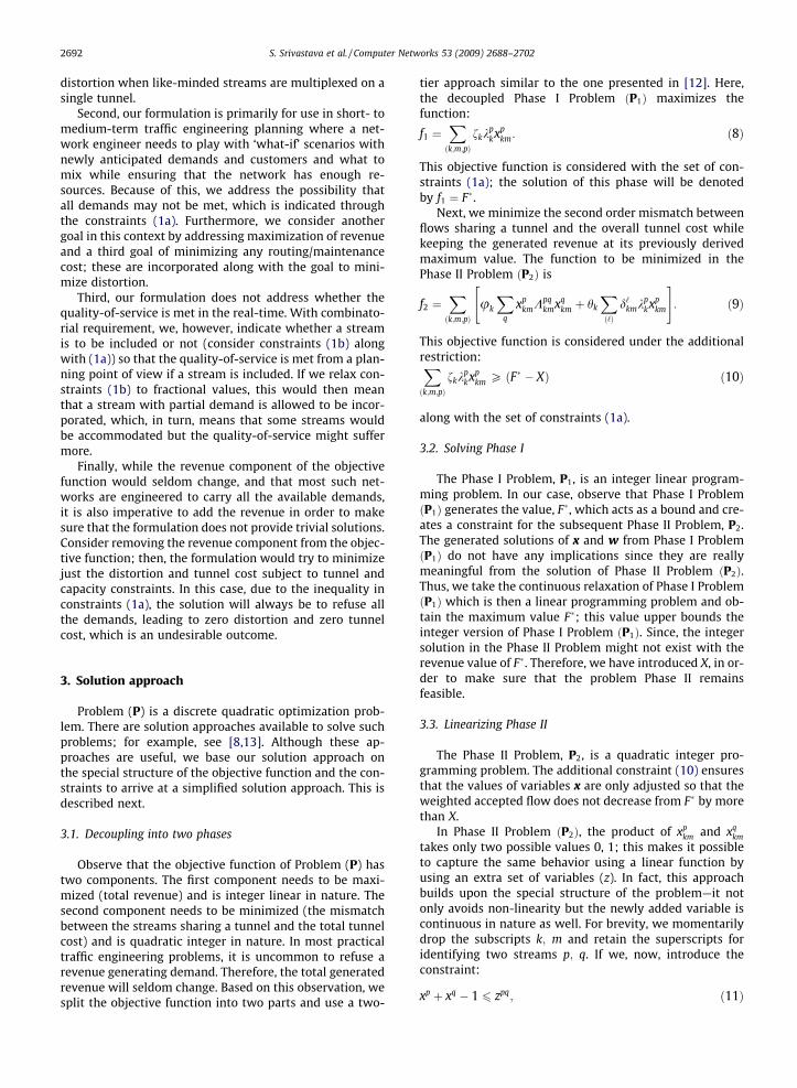
Fig. 3. Small networks: SN1 and SN2.

0

20

40

60

80

100

50 100 150 200 250 300 350 400 450

Valu

e of

εi--

-->

# of iterations --------->

SN1SN2

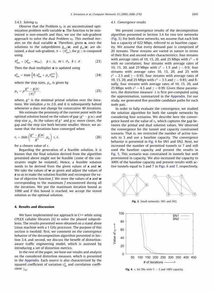
Fig. 4. �i for SNs with T‘ ¼ 3 and 100% capacity.

4. Results and discussion

We have implemented our approach in C++ while usingCPLEX callable libraries [6] to solve the phased subprob-lems. The results presented were obtained on a stand aloneLinux machine with a 1 GHz processor. The purpose of thissection is twofold: first, we comment on the convergencebehavior of the decomposition algorithm presented in Sec-tion 3.4, and second, we discuss the benefit of distortion-aware traffic engineering model, which is assessed byintroducing a set of distortion metrics.

In the rest of the paper, we base our results and analysison the considered distortion measure, which is presentedin the Appendix. Each source is also characterized by thesquared coefficient of variation c2

kp and correlation coeffi-cient ckp.

4.1. Convergence results

We present convergence results of the decompositionalgorithm presented in Section 3.4 for two test networks(Fig. 3). For both these networks, we assume that each linkhas a capacity of 622 Mbps, referred to as baseline capac-ity. We assume that every demand pair is comprised of20 streams. These streams are varied in nature in termsof their first and second order characteristics: four streamswith average rates of 10, 15, 20, and 25 Mbps with c2 ¼ 6with no correlation; four streams with average rates of10, 15, 20, and 25 Mbps with c2 ¼ 1:5 and c ¼ 0:9; fourstreams with average rates 10, 15, 20, and 25 withc2 ¼ 2:5 and c ¼ 0:95; four streams with average rates of10, 15, 20, and 25 Mbps with c2 ¼ 3:5 and c ¼ 0:85; and fi-nally, four streams with average rates of 10, 15, 20, and25 Mbps with c2 ¼ 4:5 and c ¼ 0:99. Given these parame-ters, the distortion measure K is first pre-computed usingthe approximation, summarized in the Appendix. For ourstudy, we generated five possible candidate paths for eachnode pair.

In order to fully evaluate the convergence, we studiedthe solution algorithm for both the sample networks byconsidering four scenarios. We describe here the conver-gence based on the value of �k which captures the gap be-tween the primal and dual solution values. We observedthe convergence for the tunnel and capacity constrainedscenario. That is, we restricted the number of active tun-nels to 3 and use a baseline capacity. The convergencebehavior is presented in Fig. 4 for SN1 and SN2. Next, weincreased the number of permitted tunnels to 7 and stillused the baseline capacity and present the results inFig. 5. This scenario was constrained in tunnels but wellprovisioned in capacity. We also increased the capacity to300% of the baseline capacity and present results with ac-tive tunnels equal to 3 and 7 in Figs. 6 and 7, respectively.

0

20

40

60

80

100

100 200 300 400 500 600

Valu

e of

εi--

-->


SN1SN2


0

20

40

60

80

100

100 200 300 400 500 600 700 800 900 1000

Valu

e of

εi--

-->


SN1SN2


0

20

40

60

80

100

100 200 300 400 500 600 700 800 900 1000

Valu

e of

εi--

-->


SN1SN2



From these results, we observed that for various con-strained and well-provisioned scenarios, the convergenceis achieved. Convergence of capacity constrained scenariosis particularly faster and typically require about 300–400iterations. However, for capacity well-provisioned scenar-ios, the convergence is somewhat slower for SN1 and rela-tively fast for SN2; this means that the tunnelingconstrained traffic engineering problem is somewhat moredifficult to solve than capacity constrained traffic engineer-ing problem. Observe that the values of �i decrease in steps

which can be attributed to the approach of halving theparameter q which directly affects the step sizes.

4.2. Distortion-aware traffic engineering

4.2.1. Distortion metricsTo compare Formulation (P), referred henceforth as the

Distortion-Aware-Model (DAM), against a näive allocationstrategy without distortion, referred henceforth as the Dis-tortion-Ignorant-Model (DIM), we consider the DIM to bean integer linear programming model, without the distor-tion measure term (quadratic term) in the objective func-tion. For comparison between the DAM and DIMapproaches, we have developed the following four metricsto capture the measured distortion and flow allocation:

� Metric A: Captures overall network level distortion:

A ¼Pðk;m;p;qÞx

pkmKpqxq

kmPðk;m;pÞx

pkmkp

k

: ð27Þ

� Metric B: Captures individual demand level distortion:

Bk ¼Pðm;p;qÞx

pkmKpqxq

kmPðm;pÞx

pkmkp

k

: ð28Þ

� Metric C: Captures individual active path leveldistortion:

Ckm ¼Pðp;qÞx

pkmKpqxq

kmPðpÞx

pkmkp

k

: ð29Þ

� Metric D: Compares the distortion variation in the DAMand the DIM approaches. Denote N as the number ofactive tunnels; then,

D ¼ ADIMNDIM � ADAMNDAM

NDAM � NDIM : ð30Þ

As mentioned in Section 2, distortions could be con-structed based on many different requirements; one suchexample is presented in the Appendix. These metrics cap-ture the general increase and decrease in the value of dis-tortion from a network-wide point of view.

4.2.2. Results for small networkThe first study reported is for SN1 (a six-node network).

The traffic demands and streams were the same as dis-cussed in Section 4.1. Besides the baseline capacity, we alsoconsider cases with 150% and 200% of the baseline capac-ity. To restrict tunnels on a link, we consider two tunnellimit values: 15 and 25. For comparison, we consider threedifferent values of the tunnel cost normalization parame-ter, h, at 0, 0.1, and 0.25, where h ¼ 0 means that the tunnelcost is ignored. In all studies, the normalization parameter,u, with distortion measure is set to 1 for the DAM; notethat the DIM can also be thought of as the DAM whenu ¼ 0.

We present results for Metric A in Table 3. We also in-clude in parenthesis the total number of active tunnels inthe overall network for the specified scenario. Clearly, net-work level distortion is much less with the DIM than the

Table 3Value of Metric A for small network for multiple scenarios.

Capacity (%) T‘ ¼ 15 T‘ ¼ 25

DAM DIM DAM DIM

h ¼ 0 h ¼ 0:1 h ¼ 0:25 h ¼ 0 h ¼ 0:1 h ¼ 0:25

100 2.45 (58) 3.55 (41) 3.55 (40) 5.41 (38) 1.80 (75) 3.54 (42) 3.54 (42) 4.22 (59)150 2.42 (60) 3.47 (41) 4.04 (40) 6.07 (37) 1.42 (75) 3.67 (42) 3.74 (42) 6.31 (46)200 2.54 (59) 3.59 (41) 3.58 (40) 8.35 (25) 1.48 (75) 3.62 (42) 3.56 (42) 7.74 (35)


DAM, regardless of the tunnel size. Furthermore, observethat the presence of the tunnel cost parameter ðh > 0Þleads to a significant reduction in the number of used tun-nels while the value of Metric A goes up. Note that the in-crease of h from 0.1 to 0.25, does not have appreciableimpact on the distortion. The result that provides the moststrength to the DAM approach, is that even when the num-ber of used tunnels are equal to or less than the DIM, thevalue of Metric A is less for the DAM approach.

Next we consider Metric B. In this case, we presentgraphs where the demand pair numbers are sorted basedon the value of Metric B and plotted with demands havingan increasing value of Metric B on the y-axis. In Fig. 8, wepresent Metric B for the DIM and the DAM forh ¼ 0;0:1; 0:25 when T‘ ¼ 15 and T‘ ¼ 25 for the baselinecapacity case. Observe that with higher values of T‘, thedistortion for each demand pair decreases for both theDAM and the DIM. Moreover, the values of Metric B forDIM is high and as expected, the DAM succeeds in decreas-ing the distortion for each demand. Interestingly, for

2

4

6

8

10

12

1 2 3 4 5 6 7 8 9 10 11 12 13 14 15

-----

Met

ric B

---->

# of demand pairs --------->

DIMDAM: θ=0.25

DAM: θ=0.1DAM: θ=0

2

4

6

8

10

12

1 2 3 4 5 6 7 8 9 10 11 12 13 14 15

-----

Met

ric B

---->


DIMDAM: θ=0.25


Fig. 8. Metric B with T‘ ¼ 15 and T‘ ¼ 25 and 100% capacity for smallnetwork.

T‘ ¼ 25, the differences between the DAM and the DIMfor some demand pairs is less. This can be attributed tothe capacity constrained nature of the scenario. Models(DAM or DIM) do not have many choices to allocate thestreams, rather capacity determines the available tunnelsand the allocated stream. Moreover, the value of Metric Bfor h ¼ 0:1 and h ¼ 0:25 is similar.

In Fig. 9, we list Metric B for the DIM and the DAM withh ¼ 0;0:1; 0:25 for T‘ ¼ 15 and T‘ ¼ 25; this time for the200% of the baseline capacity. Observe that the DAM pro-vides significant benefits as compared to the DIM. Whenwe compare results with the previous scenarios, we notethat the gap between the behavior of the DAM and theDIM has increased considerably. The observation suggeststhat the presence of higher amounts of capacity and tun-nels makes the DAM approach even more lucrative as com-pared to the DIM.

Next, consider Metric C which captures the distortionon each active tunnel (with positive allocated flow) forthe DAM and the DIM. For these graphs, we filter the active

2 4 6 8

10 12 14 16

1 2 3 4 5 6 7 8 9 10 11 12 13 14 15

-----

Met

ric B

---->


DIMDAM: θ=0.25


2 4 6 8

10 12 14 16

1 2 3 4 5 6 7 8 9 10 11 12 13 14 15

-----

Met

ric B

---->


DIMDAM: θ=0.25


Fig. 9. Metric B with T‘ ¼ 15 and T‘ ¼ 25 and 200% capacity for smallnetwork.

0

2

4

6

8

10

12

10 20 30 40 50 60

-----

Met

ric C

---->

# of active tunnels --------->

DIMDAM: θ=0.25


0

2

4

6

8

10

12

10 20 30 40 50 60 70 80

-----

Met

ric C

---->


DIMDAM: θ=0.25


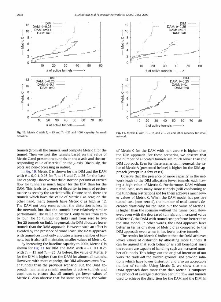
Fig. 10. Metric C with T‘ ¼ 15 and T‘ ¼ 25 and 100% capacity for smallnetwork.

0

2

4

6

8

10

12

10 20 30 40 50 60

-----

Met

ric C

---->


DIMDAM: θ=0.25


0

2

4

6

8

10

12

10 20 30 40 50 60 70 80---

-- M

etric

C --

--># of active tunnels --------->

DIMDAM: θ=0.25DAM: θ=0.1

DAM: θ=0

Fig. 11. Metric C with T‘ ¼ 15 and T‘ ¼ 25 and 200% capacity for smallnetwork.


tunnels (from all the tunnels) and compute Metric C for thetunnel. Then we sort the tunnels based on the value ofMetric C and present the tunnels on the x-axis and the cor-responding value of Metric C on the y-axis. Obviously, theplots are non-decreasing in nature.

In Fig. 10, Metric C is shown for the DIM and the DAMwith h ¼ 0;0:1;0:25 for T‘ ¼ 15 and T‘ ¼ 25 for the base-line capacity. Observe that the distortion per unit of carriedflow for tunnels is much higher for the DIM than for theDAM. This leads to a sense of disparity in terms of perfor-mance as seen by the carried traffic. On one hand, there aretunnels which have the value of Metric C as zero; on theother hand, many tunnels have Metric C as high as 12.The DAM not only ensures that the distortion is less inthe network, but that the tunnels have relatively similarperformance. The value of Metric C only varies from zeroto four (for 15 tunnels on links) and from zero to two(for 25 tunnels on link). In general, the DIM allocates fewertunnels than the DAM approach. However, such an affect isavoided by the presence of tunnel cost. The DAM approachwith tunnel cost, not only allocates a lesser number of tun-nels, but it also still maintains smaller values of Metric C.

By increasing the baseline capacity to 200%, Metric C isshown for Fig. 11 for DIM and DAM with h ¼ 0;0:1;0:25with T‘ ¼ 15 and T‘ ¼ 25. As before, the value of Metric Bfor the DIM is higher than the DAM for almost all tunnels.However, with more capacity, the DIM allocates even few-er tunnels than the previous scenario. But, the DAM ap-proach maintains a similar number of active tunnels andcontinues to ensure that all tunnels get lower values ofMetric C. Also observe that for some scenarios, the value

of Metric C for the DAM with non-zero h is higher thanthe DIM approach. For these scenarios, we observe thatthe number of allocated tunnels are much lower than theDIM approach. Even for these scenarios, in general, the va-lue of Metric A (presented before) is higher for the DIM ap-proach (except in a few cases).

Observe that the presence of more capacity in the net-work leads to the DIM allocating fewer tunnels, each hav-ing a high value of Metric C. Furthermore, DAM withouttunnel cost, uses many more tunnels (still conforming tothe tunneling restriction) and for them achieves much low-er values of Metric C. When the DAM model has positivetunnel cost (non-zero h), the number of used tunnels de-creases drastically for the DAM but the value of Metric Cis higher than the scenario without the tunnel cost. How-ever, even with the decreased tunnels and increased valueof Metric C, the DAM with tunnel cost performs better thanthe DIM model. In other words, the DAM approach faresbetter in terms of values of Metric C as compared to theDIM approach even when it has fewer active tunnels.

The results for Metric C indicate that the DAM achieveslower values of distortion by allocating more tunnels. Itcan be argued that such behavior is still beneficial sincethe routers are capable of handling such an increased num-ber of tunnels. This brings out the original intention of ourwork ‘‘to trade-off the middle ground” and provide solu-tions which have lower distortion and also an acceptablenumber of tunnels. Using Metric D, we show that theDAM approach does more than that. Metric D comparesthe product of average distortion per unit flow and tunnelsused to achieve the distortion for the DAM and the DIM. In

-0.5 0

0.5 1

1.5 2

2.5 3

3.5 4

0 100 200 300 400 500 600 700 800

-----

Met

ric B

---->


DIMDAM: θ=0.25


0.5

1

1.5

2

2.5

0 500 1000 1500 2000 2500 3000 3500 4000

-----

Met

ric C

---->


DIMDAM: θ=0.25


Fig. 12. Metrices B and C for large network.

Table 4Value of Metric D for the small network for various scenarios.

Capacity (%) T‘ ¼ 15 T‘ ¼ 25

h ¼ 0 h ¼ 0:1 h ¼ 0:25 h ¼ 0 h ¼ 0:1 h ¼ 0:25

100 3.17 20.00 31.70 7.12 �5.9 �5.9150 3.45 20.58 21.00 6.34 �34.0 �33.3200 1.72 3.85 4.37 4.00 17.0 17.34


other words, Metric D represents the differential in averagedistortion per unit flow between the DIM and the DAMnormalized by the differential in the number of activetunnels.

In Table 4, we present values for Metric D for variousscenarios for the small network. Results show that theDAM not only distributes the demands over more tunnelsbut also does intelligent allocation of streams to tunnelsleading to a smaller value of distortion as compared tothe DIM. Interestingly, the extent of benefits is variedbased on the network topology, capacity and tunnelingrestrictions. Observe that h amplifies the benefits of theDAM approach in terms of Metric A, vis-a-vis the usednumber of tunnels. The presence of tunnel cost leads tosolutions which not only use fewer tunnels (than h ¼ 0),but use these tunnels so that the distortion per unit flowis still low. When compared to the DIM, it translates intovery high values of Metric D. Moreover, at times we findthat the Metric D is negative, meaning that the DAM ap-proach for a given h uses fewer tunnels than the DIM andstill has the smaller value of the product of Metric A andnumber of used tunnels.

4.2.3. Results for large networkIn this section, we present results for a randomly gener-

ated network with 40 nodes and 77 links. We assumed thatthere are demands between every pair of nodes consistingof five streams each. These five streams have average arri-val rates of 10, 15, 20, 25, 30, c2 of 6, 1.5, 2.5, 3.5, 4.5, and cof 0, 0.9, 0.95, 0.85, 0.99, respectively. Given these param-eters, distortion measure K is first pre-computed using theapproximation given in the Appendix. We assumed thateach link has a capacity of 10 Gbps and can support 1000tunnels. The value of Metric A (and active tunnels) forthe DAM approach was found to be 0.034 (3681), 0.37(2493), and 0.37 (2464) for h equal to 0, 0.1, and 0.25,respectively. For the DIM approach, the corresponding va-lue is 0.93 (2002). In Fig. 12, we present the values of Met-ric B and C. The value of Metric D for the DAM approachwas found to be 1.03, 1.91, and 2.05 for h equal to 0, 0.1,and 0.25, respectively. The results follow the same trendas was observed for the small network.

Convergence behavior for this large network was simi-lar to the small networks discussed earlier. The computingtime on a 1 GHz processor linux machine took less than aminute to complete for this large problem. The overallsolutions approach is fast because each iteration isinexpensive.

In summary, the numerical results show that the for-mulation is indeed powerful and that it captures the basicmotive of minimizing distortion in the presence of tunnel-

ing and capacity constraints. More so, the formulation ade-quately responds to various possible scenarios of tunneland capacity restrictions. Moreover, the solution also givesa novel way of determining the optimal mapping of trafficstreams to tunnels. For the ease of forwarding, streamssharing the same tunnels can be grouped together as thesame service class. Such a grouping ensures that no addi-tional filtering needs to be done to incorporate the solutionin a real world network. Observe that such a mapping isdriven by better end-to-end performance as seen by indi-vidual streams.

5. Conclusion and future work

In this work, we presented an approach for effectivetraffic engineering of an MPLS network in the presence ofheterogeneous streams, by incorporating distortion, tun-neling limits, and capacity. Our approach is primarilyapplicable for ‘what-if’ studies for short- and medium-term traffic engineering planning, and is not geared forreal-time traffic engineering. By taking distortion into ac-count, we presented a quadratic integer programming for-mulation. We then showed how this model can belinearized. We developed an efficient two-phase algorithmto solve the traffic engineering formulation.

Our approach can be labeled as a ‘‘Distortion-Aware”traffic engineering approach. We developed several met-rics to compare our approach against a distortion-ignorantapproach. Through numerical studies, we have quantifiedthis difference and shown that our approach is quiteeffective in allocating heterogenous traffic streams to


like-minded tunnels (LSPs) to reduce distortion in a net-work-wide setting.

It may be noted that our notion of distortion is broad-based and generic. For example, if a provider does not wanttwo customers to be combined on the same tunnel, it canassign a high distortion value for this pair of customers;then, our model will identify if they are appropriate to becombined based on a set of constraints and for a givenobjective function. From our numerical results, it is evidentthat without incorporating the distortion measure, someunwanted traffic streams (or customers) may be combined.

Our approach takes an end-to-end view in addressingdistortion with traffic engineering. Several future direc-tions may be pursued. A future direction would be to allowthe ability to incorporate link level distortion. Anotherdirection would be to consider how distortion is impactedwhen there is a network failure and traffic streams are tobe re-routed. It is to be noted that the notion of distortionconsidered here is broad-based. A third future work wouldbe if typically parameters of interests such as loss, delay,and jitter could be mapped to a measure of distortionwhen traffic streams are combined in an MPLS tunnel. Fi-nally, how to incorporate any additional restrictions dueto MPLS tunnel implementation because of queues at rou-ters would be worthwhile to address.

0.850.860.870.880.890.9

0.910.920.930.940.95

8.5 9 9.5 10 10.5 11 11.5 12 12.5 13

Dis

torti

on P

[Q >

0] -

->

Approximate Distortion Λpq -->

source psource q

mean

Fig. 14. Stream p is uncorrelated.

0.830.840.850.860.870.880.890.9

0.910.920.930.94

5.5 6 6.5 7 7.5 8 8.5 9 9.5 10

Dis

torti

on P

[Q >

0] -

->


source psource q

mean

Fig. 13. Stream p is Poisson.

Acknowledgements

We thank the anonymous reviewers for their construc-tive comments that have helped improve the presentationof the paper considerably. This work was supported in partby NSF grant # CNS-0106640.

Appendix

A method (and the motivation behind this method) todetermine pair-wise distortion measure Kpq for distortionbetween two streams p and q is detailed in [15]. We brieflysummarize how it is used as input to the traffic engineer-ing problem. Given the average arrival rate ðkÞ, the squaredcoefficient of variation ðc2Þ and the coefficient of correla-tion ðcÞ, the mismatch between streams p and q is approx-imated as

Kpq ¼ Kpqr þKpq

c þKpqc ; ð31Þ

where Kpqr is the contribution of rates to the mismatch be-

tween the streams, Kpqc is the contribution due to c2, and

Kpqc due to the coefficient of correlation. These, in turn,

are estimated by

Kpqr ¼ jkp � kqj; ð32aÞ

Kpqc ¼ c2

p � 1

þ c2q � 1

�� ; ð32bÞ

and

Kpqc ¼ jðkpcqÞ þ ðkqcpÞj: ð32cÞ

A special case is when both the streams are Poisson, inwhich we set Kpq ¼ 0, since no distortion occurs.

In the remainder of this appendix, we explain the rea-son for choosing such a distortion measure. Consider that

the above mentioned streams p; q, share an exponentialserver S with an infinite queue size, and under a heavyload. Upon being served by the server S, the stream p isseparated and passed through another exponential serverSp, and we compute the value of P½Q p > 0�. Similarly, wecompute the value of P½Q q > 0� for stream q. In order toachieve this, we built upon the linear algebraic queueingtheory (LAQT) based model presented in [18]. We nowshow that higher (smaller) values of Kpq would translateinto higher (smaller) values of metric P½Q > 0� at the serv-ers. Moreover, higher values of P½Q > 0� is undesirable forany stream passing through a network since it negativelyimpacts the observed waiting time for an arriving packet.

In Figs. 13–15, we plot values of P½Q > 0� for increasingKpq (on x-axis) where stream p has different distributioncharacteristics. We consider three types arrival processesdistributions of stream p: (1) Poisson ðc2 ¼ 1Þ, (2) high c2,but uncorrelated, and (3) high c2 and correlated. Similarly,stream q varies from Poisson to uncorrelated (but withhigh c2) to correlated and high c2. In our case, a correlatedstream is approximated using [10,11] and is referred to asMarie–Mitchell with parameters k; c2, and c.

For the case when streams p is Poisson ðkpÞ and q hashigh c2 and is also correlated (i.e., q � Marie—Mitchellðkq;

c2q ; cqÞ), we present results in Fig. 13; note that eKpq is deter-

mined based on (32a) and we used kp ¼ kq ¼ 5 for thisexample. It may be noted that we observed distortions.Since, P½Q > 0� is minimal (for both streams) for lowervalues of eKpq, metric (32a) is a meaningful metric to be

0.8850.89

0.8950.9

0.9050.91

0.9150.92

0.9250.93

0.935

13 13.5 14 14.5 15 15.5 16 16.5 17 17.5 18

Dis

torti

on P

[Q >

0] -

->


source psource q

mean

Fig. 15. Stream p is correlated.


minimized in order to ensure that the distortions in thestreams are minimal. Similar patterns were observed forother values of kp and kq.

For the case when stream p is not Poisson and has ahigh c2 but is uncorrelated, and q is same as the previouscase, i.e., � Marie—Mitchellðkq; c2

q ; cqÞ, we present resultsin Fig. 14. Here, we used p � Marie—Mitchellð5;4;0Þ andfor stream q, we used kq ¼ 5 for illustration. Observe that,for this case, the suggested measure eKpq can also ade-quately capture the trend of distortion in both the streams.Similar results were obtained for streams p with different kand c2, and stream q with other values of k.

In the final case, both streams have high c2 and are alsocorrelated ðc > 0Þ. In Fig. 15, we present results for theP½Queuelength > 0� for both streams p and q as the approx-imate metric increases. For this illustration, we have usedstream p with k ¼ 5, c2 ¼ 4 and c ¼ 0:99, and stream q withk ¼ 5.

Similar behaviors were observed for different values ofk; c2 and c of the stream p, and k for stream q. To summa-rize, the chosen form of Kpq adequately captures the extentof distortion in the streams p and q. Thus, the presenteddistortion metric ðKÞ is readily available for various typesof streams under consideration to be multiplexed, and itreflects the negative impact of sharing of streams upontheir packet arrival characteristics.

It may be noted that the traffic engineering formulationpresented in this paper is independent of the distortionmeasure described above. Other methods can be developedand used while retaining the traffic engineering formula-tion presented in this paper.

References

[1] A.L. Corte, A. Lombardo, G. Schembra, Modeling superposition of on-off correlated traffic sources in multimedia applications, in:Proceedings of the IEEE INFOCOM, 1995, pp. 993–1000.

[2] A. Elwalid, C. Jin, S. Low, I. Widjaja, MATE: MPLS adaptive trafficengineering, in: Proceedings of the IEEE INFOCOM 2001, April 2001,pp. 1300–1309.

[3] A.M. Geoffrion, Lagrangean relaxation for integer programming,Mathematical Programming Study 2 (1974) 82–114.

[4] Q. He, M. Ammar, G. Riley, H. Raj, R. Fujimoto, Mapping peerbehavior to packet-level details: a framework for packet-levelsimulation of peer-to-peer systems, in: Proceedings of theMASCOTS, ACM, October 2003, pp. 71–78.

[5] M. Held, P. Wolfe, H. Crowder, Validation of sub-gradientoptimization, Mathematical Programming (1974) 62–88.

[6] Manual of Cplex Callable Libraries, ILOG Corporation, USA.[7] K. Kar, M. Kodialam, T. Lakshman, Minimum interference routing of

bandwidth guaranteed tunnels with MPLS traffic engineeringapplications, IEEE Journal on Selected Areas in Communications 18(2000) 2566–2579.

[8] Y. Li, P.M. Pardalos, K.G. Ramakrishnan, M.G.C. Resende, Lowerbounds for the quadratic assignment problem, Annals of OperationsResearch 50 (1994) 387–411.

[9] L. Lipsky, P. Fiorini, W. Hsin, A. van de Liefvoort, Auto-correlation oflag-k for customers departing from semi-Markov processes, Tech.Rep. TUM-19506, Technical University of Munich, 1995.

[10] R. Marie, Méthodes iteratives de resolution de modélesmathematiques de systémes informatiques, R.A.I.R.O.Informatique/Computing Science 12 (1978) 107–122.

[11] K. Mitchell, Constructing correlated sequence of matrix exponentialswith invariant first-order properties, Operations Research Letters 28(2001) 27–34.

[12] D. Mitra, K.G. Ramakrishnan, Techniques for traffic engineering ofmultiservice, multipriority networks, Bell Labs Technical Journal 6(2001) 139–151.

[13] P.M. Pardalos, Y. Ye, C.-G. Han, Algorithms for the solution ofquadratic knapsack problems, Linear Algebra and its Applications152 (1991) 69–91.

[14] M. Pióro, D. Medhi, Routing, Flow, and Capacity Design inCommunication and Computer Networks, Morgan KaufmannPublishers, 2004.

[15] S. Srivastava, Models and algorithms for effective traffic engineeringof tunnel-based backbone networks, Ph.D. Dissertation, ComputerScience and Electrical Engineering Department, University ofMissouri–Kansas City, 2004.

[16] S. Srivastava, B. Krithikaivasan, D. Medhi, M. Pióro, Trafficengineering in the presence of tunneling and diversity constraints:formulation and Lagrangean decomposition approach, in:Proceedings of the 18th International Teletraffic Congress, ElsevierScience, Berlin, 2003, pp. 461–470.

[17] S. Srivastava, D. Medhi, Traffic engineering of tunnel-based networkswith class specific diversity requirements, Journal of CombinatorialOptimization 12 (2006) 97–125.

[18] S. Srivastava, K. Mitchell, A. van de Liefvoort, Correlations induced ina packet stream by background traffic in a multiplexed environment,in: Proceedings of the 18th International Teletraffic Congress (ITC),Elsevier Science, Berlin, 2003, pp. 511–520.

[19] S. Srivastava, S.R. Thirumalasetty, D. Medhi, Network trafficengineering with varied levels of protection in the next generationInternet, in: A. Girard, B. Sansò, F. Vazquez-Abad (Eds.), PerformanceEvaluations and Planning Methods for the Next Generation Internet,Springer, 2005, pp. 99–124.

[20] C.-F. Su, G. deVeciana, Statistical multiplexing and mix-dependentalternate routing in multiservice networks, IEEE/ACM Transactionson Networking 8 (2000) 99–108.

[21] X. Xiao, A. Hannan, B. Bailey, L. Ni, Traffic engineering with MPLS inthe Internet, IEEE Network 14 (2) (2000) 28–33.

[22] S. Yasukawa, A. Farrel, O. Komolafe, An analysis of scaling issues inMPLS-TE core networks, IETF RFC 5439, February 2009. <http://www.rfc-editor.org/rfc/rfc5439.txt>.

Shekhar Srivastava received his B.Tech.degree in Electronics and CommunicationEngineering at the College of Technology ofPant University, Pantnagar, India and M.E.degree in Telecommunication at the IndianInstitute of Science, Bangalore, Karnataka,India and a Ph.D. in Computer Networkingand Telecommunication Networking fromUniversity of Missouri–Kansas City, MO, Uni-ted States. He has worked on performance andengineering of wireless handsets and systemsat SasKen Communication Technologies,

Bangalore, India. As a post-doc at the University of Montreal, Canada, heworked on performance models for design of IP networks. He has alsoworked on design and optimization of wireless backhaul networks at
Schema Inc. He currently works on next generation wireless technologiesat Huawei Technologies. His areas of interest are performance modeling,design and optimization of systems related to computer and communi-cation networks.
http://www.rfc-editor.org/rfc/rfc5439.txt

http://www.rfc-editor.org/rfc/rfc5439.txt


Appie van de Liefvoort is a Professor andChair of the Department of Computer ScienceElectrical Engineering at the University ofMissouri–Kansas City, where he has beensince 1987. Prior to joining UMKC, he was afaculty member at the University of Kansas.He received graduate degrees in ComputerScience and Mathematics from the Universityof Nebraska–Lincoln, and from the KatholiekeUniversiteit in Nijmegen, The Netherlands,respectively. His research interests includeQueueing Theory and performance modeling

of computer and communication networks, specializing in linear alge-braic queueing theory, the matrix-exponential distribution, and corre-lated matrix-exponential sequences.

Deep Medhi is Professor of Computer Net-working, Computer Science and ElectricalEngineering Department at the University ofMissouri–Kansas City, United States. Hereceived B.Sc. (Hons) in Mathematics fromCotton College/Gauhati University, India,M.Sc. in Mathematics from the University ofDelhi, India, and Ph.D. in Computer Sciencesfrom the University of Wisconsin–Madison,United States. Prior to joining UMKC in 1989,he was a member of technical staff at AT&TBell Laboratories. He was an invited visiting

professor at the Technical University of Denmark and a visiting researchfellow at Lund Institute of Technology, Sweden. He is a Fulbright senior

specialist. His research interests are resilient multi-layer network design,network routing and design, sensor networks. He has published overeighty papers, and is co-author of the books, Routing, Flow, and CapacityDesign in Communication and Computer Networks (2004), and NetworkRouting: Algorithms, Protocols, and Architectures (2007), both publishedby Morgan Kaufmann Publishers.

Documents

Traffic engineering of MPLS backbone networks in the presence of heterogeneous streams