USDOT Region V Regional University Transportation Center Final Report

IL IN

WI

MN

MI

OH

NEXTRANS Project No. 088OY04

Traffic Behavior at Freeway Bottlenecks

By

Benjamin Coifman, PhD

Associate Professor The Ohio State University

Department of Civil, Environmental, and Geodetic Engineering Department of Electrical and Computer Engineering

Hitchcock Hall 470 2070 Neil Ave, Columbus, OH 43210

E-mail: Coifman.1@OSU.edu

and

Seoungbum Kim, PhD Department of Transportation and Logistics Engineering

Hanyang University at Ansan

DISCLAIMER

Funding for this research was provided by the NEXTRANS Center, Purdue University under Grant No. DTRT07-G-005 of the U.S. Department of Transportation, Research and Innovative Technology Administration (RITA), University Transportation Centers Program. The contents of this report reflect the views of the authors, who are responsible for the facts and the accuracy of the information presented herein. This document is disseminated under the sponsorship of the Department of Transportation, University Transportation Centers Program, in the interest of information exchange. The U.S. Government assumes no liability for the contents or use thereof.

USDOT Region V Regional University Transportation Center Final Report

TECHNICAL SUMMARY

IL IN

WI

MN

MI

OH

NEXTRANS Project No. 088OY04 Final Report, September 23, 2014

Traffic Behavior at Freeway Bottlenecks

Introduction This study examines traffic behavior in the vicinity of a freeway bottleneck, revisiting commonly held assumptions and uncovering systematic biases that likely have distorted empirical studies of bottleneck formation, capacity drop, and the fundamental relationship (FR). This simulation-based study examines an on-ramp bottleneck using Newell's lower order car following model with a driver relaxation factor added for the vehicles that enter or are immediately behind an entering vehicle (termed "affected vehicles"). The affected vehicles will tolerate a truncated headway for a little while after an entrance but slowly relax back to their preferred speed-spacing relationship. All other vehicles remain on their preferred speed-spacing relationship throughout.

Simulating conventional detector measurements, we show that flow is supersaturated in any sample containing an affected vehicle with a truncated headway, i.e., the flow is higher than the underlying FR would predict. This systematic bias is not readily apparent in the detector measurements, during the initial queue formation speeds remain close to free speed and the supersaturated states can exceed the bottleneck capacity. As the affected drivers relax, the high flows become unsustainable so a queue initially forms downstream of the on-ramp (consistent with earlier empirical results) only later receding upstream past the on-ramp. This initial phase of activation often lasts several minutes. Without any evidence of queuing upstream of the ramp, the conventional point bottleneck model would erroneously indicate that the bottleneck is inactive. Thus, an empirical study or traffic responsive ramp meter could easily mistake the supersaturated flows to be the bottleneck's capacity flow, when in fact these supersaturated flows simply represent system loading during the earliest portion of bottleneck activation. Instead of flow dropping "from capacity", we see flow drop "to capacity" from supersaturation. We also discuss how the supersaturated states distort empirically observed FR. We speculate that these subtle mechanisms are very common and have confounded the results of many past empirical studies.

Findings This simulation study examined traffic behavior in the vicinity of an on-ramp bottleneck, revisiting commonly held assumptions and uncovering systematic biases that likely have distorted empirical studies of bottleneck formation, capacity drop, and the fundamental relationship. We modify Newell's car following model to include the driver relaxation process. At the macroscopic scale the traffic state for any sample containing one or more of these relaxing vehicles will be supersaturated. So here is a

NEXTRANS Project No 019PY01Technical Summary - Page 1

reproducible mechanism that can pull the empirical flow density fundamental relationship (qkFR) above the underlying qkFR, i.e., shifting away from the origin, and in some cases, above the roadway capacity (RCap) at the apex of the qkFR.

As an on-ramp bottleneck becomes active, the entering drivers are constantly being replenished, and keep the traffic state supersaturated. After the combined demand first exceeds capacity in our simulations, the bottleneck activation progresses through the following steps: (1) 10-30 sec of moving bottlenecks downstream of the on-ramp, superficially indistinguishable from high flow, non-active conditions, but the supersaturated q is above RCap. (2) A fixed queue forms some distance downstream of the on-ramp and eventually extends up to 1.8 miles beyond the ramp. Between the on-ramp and d-end, the supersaturated q remains above RCap (beyond the d-end, q never exceed RCap). (3) The u-end grows upstream, eventually reaching the on-ramp 200-300 sec after demand first exceeded capacity. (4) With the ramp drivers now entering at lower speeds, the relaxation distance shrinks, and thus, the d-end recedes upstream. The number of vehicles stored downstream drops, and as they dissipate, they consume some RCap that would otherwise be available at the ramp, i.e., q drops below RCap upstream of the d-end. (5) Finally the system stabilizes at RCap (or near RCap in the presence of stochastic ramp arrivals). Steps 1-3 are termed the loading period and step 4 the settling period; both of these periods exhibit supersaturated traffic states downstream of the on-ramp, though during the settling period q is below RCap. The time scales for these events are likely to be longer in more realistic scenarios.

Reinterpreting many empirical studies in the context of our results, during the loading period a conventional point bottleneck model would erroneously indicate that the bottleneck is inactive. In fact during the loading period most of the bottleneck activity actually occurs downstream of the on-ramp, which is inconsistent with a simple point bottleneck model. The bottleneck process occurs over an extended distance, in excess of 1 mile. If one fails to recognize the fact that the bottleneck is already active during the loading period, one would overestimate the bottleneck capacity due to the supersaturated q and the recorded activation time will be too late. Only after the settling period is over does q return to the actual bottleneck capacity, which is equal to RCap. Instead of q dropping "from capacity", we see q drop "to capacity" from supersaturation. If proven empirically, this finding has important implications for traffic flow theory and traffic control, e.g., understanding the bottleneck process and applying traffic responsive ramp metering, respectively.

We suspect these confounding effects have largely gone unnoticed due to the ambiguity in defining exactly what constitutes "unqueued" conditions. In fact, measuring q, k, v from our simulation results we see a seemingly parabolic qkFR more than a mile downstream of the on-ramp due to the driver relaxation, with the parabolic portion coming from the supersaturated states above RCap, i.e., these locations are not strictly downstream of the bottleneck process, and v is only slightly below vf. However, as previously argued by Coifman and Kim (2011) any v below vf may be indicative of a sample that includes queued conditions for a portion of the sample and that appears to be the case in the current study as well: as long as a driver is traveling below vf they are constrained by downstream conditions. Thus, using a strict vf criteria for unqueued states would ensure the downstream observation site was past the entire bottleneck process, but it would also put this site at least a mile past the on-ramp in

NEXTRANS Project No 019PY01Technical Summary - Page 2

many of our simulations- a distance that is often infeasible due to extraneous features downstream of the on-ramp that likely impact the measurements in empirical studies.

Recommendations The driver relaxation process is a confounding factor far below the resolution of conventional macroscopic data, and empirical studies usually fail to account for it. One thing is clear, however, the bottleneck process appears to occur over a much longer distance than previously thought, with subtle influences arising miles beyond the apparent point bottleneck location. To advance the understanding of the bottleneck mechanisms, our community needs to devise ways to better handle multiple interacting features rather than assuming a simple point bottleneck. Right now we are faced with the very daunting challenge that there are few data sources with high enough resolution to tease out the individual contributing factors and enable such advances. So the present work is also meant to help focus future data collection in such a way that these necessary data will be collected from the right locations, and ultimately, so that more robust models can eventually developed. None of the existing publicly available, microscopic, empirical traffic data sets span the necessary region (up to two miles downstream of the apparent bottleneck). Furthermore, conventional traffic flow theories should be evaluated in the context of the new findings. Ultimately understanding the nuances of the bottleneck process is key to alleviating congestion and increasing throughput on the nation's freeways.

Contacts For more information:

Benjamin Coifman, PhD The Ohio State University Department of Civil, Environmental, and Geodetic Engineering Hitchcock Hall 470 2070 Neil Ave, Columbus, OH 43210

(614) 292-4282 Coifman.1@OSU.edu

https://ceg.osu.edu/~coifman

NEXTRANS Center Purdue University - Discovery Park 3000 Kent Ave West Lafayette, IN 47906

nextrans@purdue.edu (765) 496-9729 (765) 807-3123 Fax

www.purdue.edu/dp/nextrans

NEXTRANS Project No 019PY01Technical Summary - Page 3

i

TABLE OF CONTENTS

Page

LIST OF FIGURES ........................................................................................................... iii  

LIST OF TABLES ............................................................................................................. iv  

CHAPTER 1. INTRODUCTION ....................................................................................... 1  

1.1   Overview ............................................................................................................... 3  

CHAPTER 2. MODELING THE CAR FOLLOWING AND DRIVER RELAXATION

PROCESSES ..................................................................................................................... 5  

2.1   Terminology .......................................................................................................... 5  

2.2   Car following model .............................................................................................. 6  

2.3   Driver relaxation model ......................................................................................... 6  

CHAPTER 3. NUMERICAL ANALYSIS ....................................................................... 10  

3.1   Queue formation near the on-ramp ...................................................................... 11  

3.2   Defining the loading and settling periods ............................................................ 13  

3.3   Alternative scenarios ........................................................................................... 15  

3.4   Stochastic ramp arrivals ...................................................................................... 15  

3.5   Model calibration and other models .................................................................... 16  

CHAPTER 4. DISCUSSION ............................................................................................ 26  

4.1   Bottleneck capacity ............................................................................................. 26  

4.2   The fundamental relationship .............................................................................. 30  

ii

4.3   More realistic details ........................................................................................... 32  

CHAPTER 5. CONCLUSIONS ....................................................................................... 38  

REFERENCES ................................................................................................................. 41  

iii

LIST OF FIGURES

Figure Page

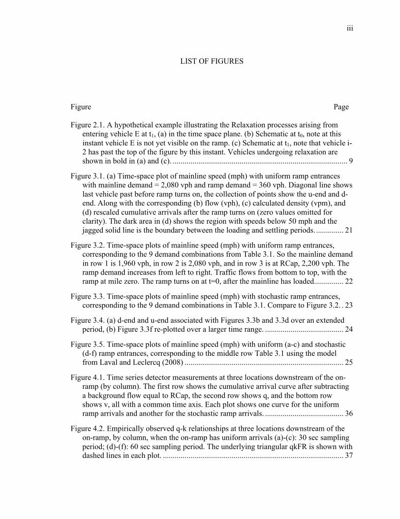
Figure 2.1. A hypothetical example illustrating the Relaxation processes arising from entering vehicle E at t1, (a) in the time space plane. (b) Schematic at t0, note at this instant vehicle E is not yet visible on the ramp. (c) Schematic at t1, note that vehicle i-2 has past the top of the figure by this instant. Vehicles undergoing relaxation are shown in bold in (a) and (c). ......................................................................................... 9  

Figure 3.1. (a) Time-space plot of mainline speed (mph) with uniform ramp entrances with mainline demand = 2,080 vph and ramp demand = 360 vph. Diagonal line shows last vehicle past before ramp turns on, the collection of points show the u-end and d-end. Along with the corresponding (b) flow (vph), (c) calculated density (vpm), and (d) rescaled cumulative arrivals after the ramp turns on (zero values omitted for clarity). The dark area in (d) shows the region with speeds below 50 mph and the jagged solid line is the boundary between the loading and settling periods. .............. 21  

Figure 3.2. Time-space plots of mainline speed (mph) with uniform ramp entrances, corresponding to the 9 demand combinations from Table 3.1. So the mainline demand in row 1 is 1,960 vph, in row 2 is 2,080 vph, and in row 3 is at RCap, 2,200 vph. The ramp demand increases from left to right. Traffic flows from bottom to top, with the ramp at mile zero. The ramp turns on at t=0, after the mainline has loaded. .............. 22  

Figure 3.3. Time-space plots of mainline speed (mph) with stochastic ramp entrances, corresponding to the 9 demand combinations in Table 3.1. Compare to Figure 3.2. . 23  

Figure 3.4. (a) d-end and u-end associated with Figures 3.3b and 3.3d over an extended period, (b) Figure 3.3f re-plotted over a larger time range. ........................................ 24  

Figure 3.5. Time-space plots of mainline speed (mph) with uniform (a-c) and stochastic (d-f) ramp entrances, corresponding to the middle row Table 3.1 using the model from Laval and Leclercq (2008) ................................................................................. 25  

Figure 4.1. Time series detector measurements at three locations downstream of the on-ramp (by column). The first row shows the cumulative arrival curve after subtracting a background flow equal to RCap, the second row shows q, and the bottom row shows v, all with a common time axis. Each plot shows one curve for the uniform ramp arrivals and another for the stochastic ramp arrivals. ........................................ 36  

Figure 4.2. Empirically observed q-k relationships at three locations downstream of the on-ramp, by column, when the on-ramp has uniform arrivals (a)-(c): 30 sec sampling period; (d)-(f): 60 sec sampling period. The underlying triangular qkFR is shown with dashed lines in each plot. ............................................................................................ 37

iv

LIST OF TABLES

Table Page

Table 3.1. Combined demand from mainline and ramp flow. .......................................... 19  

1

CHAPTER 1. INTRODUCTION

Empirical bottleneck studies are encumbered with the difficult challenge of

simultaneously measuring bottleneck capacity (BCap), identifying the time that the

bottleneck becomes active (i.e., starts restricting flow), and establishing where the

bottleneck actually forms. In this report we show that an on-ramp bottleneck's activation

may occur several minutes earlier than conventional bottleneck models would detect, and

that unsustainably high flows after the true activation time could easily be mistaken for

BCap, leading to an overestimate of capacity. In the present case these discrepancies arise

due to driver relaxation, whereby a driver will accept a short headway for some time

(often 20 sec or more, e.g., Smith, 1985) so that they can enter a lane that is constrained

by downstream conditions and then will slowly "relax" to their preferred headway (e.g.,

Newman, 1963; Cohen, 2004; Leclercq et al., 2007; Wang and Coifman, 2008; Xuan and

Coifman, 2012). Likewise, the driver immediately behind an entrance will slowly relax in

response to their newly shortened headway. Of course average headway is the reciprocal

of flow, q, so as drivers relax q should drop.

Typically BCap is defined as the highest sustained throughput and it is usually

observed immediately prior to activation. Many researchers have observed a capacity

drop where discharge flow drops immediately after the bottleneck becomes active (e.g.,

Banks, 1990; Hall and Agyemang-Duah, 1991; Persaud et al., 1998; Cassidy and Bertini,

1999; Zhang and Levinson, 2004; Chung et al., 2007; Duret et al., 2010; Leclercq et al.,

2011). Several studies have stressed the importance of measuring BCap downstream of

the bottleneck to avoid including demand in excess of capacity upstream of a growing

queue and doing so without any intervening ramps to ensure that the entire throughput is

measured (e.g., Hurdle and Datta, 1983; Hall and Agyemang-Duah, 1991, Cassidy and

2

Bertini, 1999). Most contemporary studies employ the point bottleneck model, wherein

the bottleneck process is assumed to occur over a negligible distance along the roadway

(e.g., Daganzo, 1997; Zhang and Levinson, 2004). In this case an active bottleneck is

defined as a point on the network with queuing upstream and unqueued conditions

downstream (see, e.g., Bertini and Leal, 2005). A few studies model the bottleneck

process over space, either by assuming multiple point bottlenecks (e.g., Banks 1989; Hall

and Hall, 1990) or that the bottleneck process itself occurs over an extended distance

(e.g., Hurdle and Datta, 1983; Hall et al., 1992; Coifman and Kim 2011). There are also

many different techniques used to determine when a bottleneck is active:

[a1] some studies look for a speed drop upstream of the bottleneck, indicative of

queuing (e.g., Banks, 1990; Hall and Agyemang-Duah, 1991);

[a2] some look for a positive correlation between flow and occupancy, indicative of

the traffic state falling in the unqueued regime of the fundamental relationship

(e.g., Hall and Agyemang-Duah, 1991). Both a1 and a2 have latency, requiring

the queue to grow back to the detection location before the queuing can be

detected.

[a3] More recently Cassidy and Bertini, (1999) used rescaled cumulative arrival

curves to construct a queuing diagram and measure accumulation between

detector stations (thus identifying queuing before the queue reaches a detector

station) and verified that the locally observed conditions at the stations were

consistent with a1 and a2.

Most bottleneck studies do not account for driver relaxation and this report seeks

to demonstrate that driver relaxation is an important factor that can confound the results

of empirical studies if it is not accounted for. We argue that if drivers are perpetually

entering the freeway from an on-ramp, then the maximum sustainable throughput should

drop as a function of distance downstream of the on-ramp due to driver relaxation.

Although throughput becomes more constrained as drivers relax, traffic downstream of

the on-ramp should be traveling at or near free speed, vf, even after this relaxation starts

limiting throughput. The simulations presented herein show that this relaxation process

3

can extend at least 1.8 mi downstream of the on-ramp, much further beyond the ramp

than most empirical studies contemplate. The initial period of activation is characterized

by very minor accumulations downstream of the on-ramp that are below the sensitivity of

a1-a3. Then as congestion worsens, these downstream accumulations dissipate as the

queue moves largely upstream of the on-ramp. A detailed discussion of these impacts will

be presented in Section 3. Needless to say, this view implicitly assumes that the on-ramp

bottleneck process occurs over an extended distance and should not be modeled as a

single point bottleneck.

A few empirical studies have explicitly considered driver relaxation at on-ramps

and support the general need to account for driver relaxation. Cohen (2004) demonstrated

that applying different sensitivity values into the existing FRESIM model to account for

the relaxation process can yield better consistency with field data compared to the un-

relaxed procedure. Leclercq et al. (2007) studied an on-ramp that was subject to queuing

from a downstream bottleneck and found impacts from driver relaxation similar to those

that we find herein when the on-ramp is the source of the bottleneck (Laval and Leclercq,

2008, subsequently developed a model of Leclercq et al's observations). Daamen et al.

(2010) found evidence of driver relaxation at an on-ramp bottleneck, but only undertook

a detailed study of the vehicles in the merge area while the relaxation process extended

beyond the downstream end of their study segments.

1.1 Overview

The remainder of this report is as follows. Section 2 reviews the underlying

models used in the study. We seek the simplest model that can demonstrate the effects,

and to this end we extend the lower order car following model by Newell (2002) to

include driver relaxation for those affected drivers directly involved with an entrance

maneuver (an entering driver or the driver immediately behind an entering vehicle).

Section 3 uses simulation to investigate the systematic impact of driver relaxation at an

on-ramp bottleneck on a one-lane freeway. As such, we explicitly exclude other

important factors, e.g., lane change maneuvers within the bottleneck (Coifman et al.,

4

2003; Laval and Daganzo, 2006; Duret et al., 2010; Coifman and Kim, 2011). So the

present work should not be viewed as a complete model of the very complicated

bottleneck process, rather, these results are intended to highlight the impacts of what we

believe to be an important factor that has previously gone largely overlooked. The report

closes with a discussion in Section 4 and conclusions in Section 5.

5

CHAPTER 2. MODELING THE CAR FOLLOWING AND DRIVER RELAXATION

PROCESSES

This study uses microscopic simulation to provide insight into empirically

observed macroscopic phenomena. This section presents the details of the microscopic

car following and relaxation models used in this study. After the bottleneck activates all

vehicles passing the on-ramp will spend a portion of time car following. While all of

these vehicles will be delayed by downstream conditions, only a few affected vehicles

will be impacted directly by the entrances: an entering vehicle and the vehicle

immediately behind an entering vehicle (e.g., vehicles E and i, respectively, in Figure

2.1). The remainder of this section briefly reviews key terminology used in this report,

the car following model, and then the relaxation model used for the affected vehicles.

2.1 Terminology

Before proceeding, it is important to define several key terms. The traffic state

(flow, q, density, k, and space mean speed, v) is commonly assumed to fall on some

fundamental relationship, FR, that may vary over time and space. However, perturbations

can cause the traffic state to deviate from the underlying FR, e.g., the shock due to the

arrival of a queue from downstream. The FR is commonly characterized in terms of a

bivariate relationship between two of the three parameters1. In our discussion, we will

refer to the flow-density curve, qkFR, one of the three commonly used bivariate

realizations of the FR. We assume a triangular qkFR (e.g., as found in Munjal et al.,

1971; Hall et al., 1986; Banks, 1989), which has several key parameters: the wave speed,

w, corresponding to the slope of the queued regime, the free speed, vf, corresponding to

1 In each case the third parameter can be calculated from the fundamental equation.

6

the slope of the unqueued regime, and capacity. Unfortunately, capacity means several

different things in the context of freeway flow. On the one hand, there is the maximum

throughput that an infinitesimally short segment of road can accommodate if provided

sufficient demand from upstream and no queuing downstream. This parameter

corresponds to q at the apex of the qkFR and we call it the roadway capacity, RCap,

since it characterizes the particular point along the roadway. Although RCap exists at all

locations, at most locations one should rarely see q that high (see, e.g., Figure 6 in Hall et

al., 1992). On the other hand, in Section 1 we spoke strictly of BCap, the maximum

sustainable throughput past a bottleneck. In a point bottleneck model BCap would simply

be the smallest RCap over many successive infinitesimally short segments, and this

minimum RCap would occur at the assumed point bottleneck location. In an extended

bottleneck model we use BCap as shorthand to capture all of the factors that contribute to

the bottleneck capacity.

2.2 Car following model

This study uses Newell's lower order car following model, which implicitly

assumes an underlying triangular qkFR (Newell, 2002). Ultimately, the following vehicle

replicates the lead vehicle's trajectory, shifted in time and space by w. Under this model a

driver is in car following mode whenever speed is below vf, otherwise they travel at vf if

the spacing is Scrit = vf / RCap or larger. Although the model has few parameters, it has

proven to be very robust, e.g., Ahn et al. (2004), while Coifman (2002) used the same

shifting technique to accurately estimate vehicle trajectories and travel times over

extended links within a queue.

2.3 Driver relaxation model

Consider vehicle i at t0 in Figure 2.1, this vehicle is traveling at vf and spacing in

excess of Scrit. Thus, at this instant the driver is not car following and the local,

macroscopic traffic state is unqueued. Then at t1 vehicle E enters the freeway from an on-

ramp, immediately ahead of i. Both vehicles are now below their preferred spacing for

the given speed. The drivers will change speed to correct their spacing and slowly relax

7

back to their preferred speed-spacing relationship over time (often 20 sec or more) and

space.

In our study, whenever a following vehicle's spacing is shorter than preferred, the

vehicle will respond depending on the relative spacing. If the spacing is increasing over

time because the lead vehicle is traveling faster, then the follower will maintain its initial

speed until achieving the desired spacing and then will resume conventional car

following (e.g., vehicle E from t1 to tn in Figure 2.1). Otherwise, if the lead vehicle is

traveling slower than the following vehicle, the follower will decelerate until they reach a

speed such that the relative spacing is increasing and then they will maintain that speed

until they reach their preferred speed-spacing relationship, e.g., vehicle i in Figure 2.1.

The simulation checks the spacing, Si(t), for vehicle i and finds that it decreases from

time step t1 to time step t2, i.e., Si(t2) < Si(t1). At this point the vehicle starts decelerating

at a fixed rate, dcc, i.e., ai(t2) = -dcc. If in the next time step the spacing continues to

decrease, then the vehicle increases its deceleration rate by another dcc, ai(t3) = ai(t2)-dcc.

This deceleration is repeated each time step until either the spacing starts increasing or

the vehicle reaches its preferred speed-spacing relationship. In the case of vehicle i, the

spacing starts to increase at tm, so the vehicle stays at a constant speed from tm until

reaching its preferred speed-spacing relationship at tk, and then the vehicle will begin car

following. The portions of the trajectories subject to the relaxation process are shown

with bold curves in Figure 2.1a. Equation 1 shows the process of updating the speed and

position during the relaxation process for some simulated vehicle k. Finally, for this

simulation the vehicles enter from the on-ramp anticipating the fact that they are

beginning the relaxation process, so they enter the mainline at a speed that is a fixed

amount, dv, slower than their new leader, with zero acceleration, e.g., in Figure 2.1, vE(t1)

= vi-1(t1)-dv and aE(t1)=0.

8

𝑥! 𝑡 + 𝑑𝑡 = 𝑥! 𝑡 + 𝑣! 𝑡 𝑑𝑡 + !!𝑎! 𝑡 𝑑𝑡

!

𝑣! 𝑡 + 𝑑𝑡 = 𝑣! 𝑡 + 𝑎! 𝑡 𝑑𝑡 (1)

𝑎! 𝑡 + 𝑑𝑡 = 0, 𝑆! 𝑡 + 𝑑𝑡 > 𝑆! 𝑡𝑎! 𝑡 − 𝑑𝑐𝑐, 𝑜𝑡ℎ𝑒𝑟𝑤𝑖𝑠𝑒

Where, 𝑥! 𝑡 = the position of the kth vehicle at time t 𝑣! 𝑡 = the speed of the kth vehicle at time t 𝑎! 𝑡 = the acceleration of the kth vehicle at time t 𝑆! 𝑡 = the spacing from the kth vehicle to its leader at time t 𝑑𝑡 = time step of the simulation 𝑑𝑐𝑐 = unit rate of deceleration

Note that except for the entering vehicles and those immediately behind an

entering maneuver, by definition the car following model from Section 2.2 ensures the

drivers will maintain their preferred headway, and thus, will not be subject to this

relaxation process. Although there are only a few affected vehicles that undergo the

relaxation process, during queued conditions each affected vehicle defines a new

"prototype" trajectory for all subsequent vehicles to follow, as per Section 2.2. For

example, vehicle i+1 in Figure 2.1a starts out in unqueued conditions, but it catches up to

vehicle i at tb. At this point vehicle i+1 begins car following, i.e., it follows the same

trajectory as vehicle i, shifted in time and space by w. Vehicle i+1 ceases car following

when it finally returns to vf, and it does so at Scrit.

9

Figure 2.1. A hypothetical example illustrating the Relaxation processes arising from

entering vehicle E at t1, (a) in the time space plane. (b) Schematic at t0, note at this instant

vehicle E is not yet visible on the ramp. (c) Schematic at t1, note that vehicle i-2 has past

the top of the figure by this instant. Vehicles undergoing relaxation are shown in bold in

(a) and (c).

  (a)

Time  

W  

W  vf  

W  

at  t0   at  t1  

i  

E  

i-­‐1  

Direction  of  travel  

i-­‐2  

i-­‐1  

i  

(b) (c) Vehicle  i  Vehicle  i-­‐2  Distance  

On-­‐ramp  

t0  

Trajectories  undergoing  relaxation    

t2   tk  

vf  

tm  

Vehicle  E   Vehicle  i+1  

tb  

Trajectory  derived  by    leader    

tn  t1  

Vehicle  i-­‐1  

10

CHAPTER 3. NUMERICAL ANALYSIS

This section simulates traffic past an on-ramp using the models from Section 2

applied to a one-lane freeway section with vf = 60 mph, RCap = 2,200 vph, and w = -12

mph. There is an on-ramp at mile 0 and the mainline segment is long enough to ensure

that no queuing reaches either end. Point queues are allowed to form on the ramp

whenever the ramp demand cannot be met. All vehicles are homogeneous, with identical

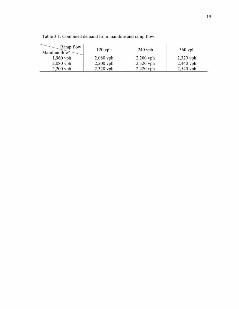
driving characteristics (vf, dcc, etc.). The model is tested under nine combinations of

mainline and ramp flow: (1,960 vph, 2,080 vph, 2,200 vph) x (120 vph, 240 vph, 360

vph), as shown in Table 3.1. Note that the largest mainline demand is equal to RCap, and

that the combined demand is below RCap in one case, equal to RCap in two, and above

RCap in the remaining six. For the sake of clarity (i.e., limiting extraneous noise) the

mainline has strictly uniform arrivals in the presented results, a point we will revisit in

Section 4.3. The ramp is evaluated both with uniform and stochastic arrivals. When

vehicles enter from the ramp, they do so at the midpoint between two mainline vehicles,

thus, the two affected vehicles initially have the same spacing. Due to a lack of empirical

calibration data, we are forced to use a heuristic method to set dv and dcc for the affected

vehicles. This section presents the results for dv = 1 mph and dcc = 2 ft/sec2, though we

considered other values for each parameter, as summarized in Section 3.5. Each

simulation includes 4,000 mainline vehicles. The on-ramp flow is held at zero until 100

sec after the first mainline vehicle passes the on-ramp, allowing the mainline to stabilize

before any on-ramp vehicles enter. Then at t=0 the on-ramp abruptly begins flowing at

the set rate. First we present the results for uniform arrivals on the ramp, and then for

stochastic arrivals. The simulation time step, dt, is 0.2 sec.

11

3.1 Queue formation near the on-ramp

Figure 3.1a shows a gray scale plot of the mainline speed (from the individual

vehicle trajectories) in the time-space plane with mainline demand of 2,080 vph and

uniform ramp arrivals at 360 vph. Traffic flows from bottom to top. Each measurement is

calculated from the individual vehicle trajectories using a moving average every 5 sec

over a time window of 31.1 sec2 at every 0.1 mile. In this case v is the harmonic average

of the individual vehicle speeds passing the given location. As shown in the color bar, the

lighter the color the faster the speed, and the white region corresponds to vf. The plot also

shows two points from each delayed trajectory, indicating the location where the vehicle

first drops below vf and then the location where the vehicle first returns to vf. Taken

collectively, these two groups of points respectively define the envelope of the upstream

end of the queue, u-end, and downstream end of the queue, d-end (avoiding the more

common, but ambiguous terms, "head" and "tail"). The straight line passing through the

origin is the trajectory of the last mainline vehicle before the on-ramp starts flowing.

Figures 3.1b-c show the corresponding q, and k, respectively, where q comes from the

number of vehicles per sample and k is calculated via the fundamental equation, k = q/v.3

Starting at t=0 the combined ramp and mainline demand exceeds RCap and the

bottleneck becomes active, but because of the driver relaxation process the first several

minutes of activation does not exhibit any clear indicators of queuing. Flows in excess of

RCap are common during these first few minutes after activation and the labels are

shown with a dark background in Figure 3.1b (some flows are 250 vph over RCap, i.e.,

11% above RCap). Over this region q and k remain positively correlated (as will be

shown in Section 4.2), thus, precluding timely detection via a2 from Section 1. The

shaded area in Figure 3.1d shows the region where speeds are below 50 mph. Speeds

remain above 50 mph everywhere until 3.3 min after the bottleneck activates and the first

location where speed drops below 50 mph is downstream of the ramp. It takes several

2 This unusual period is used simply to prevent aliasing in the flow at RCap due to samples with partial headways. 3 The moving average is centered on the reported time, as a result the plots are non-causal, the impacts of an event start

becoming evident 15.5 sec before the event; which is why q starts increasing shortly before the on-ramp starts flowing.

12

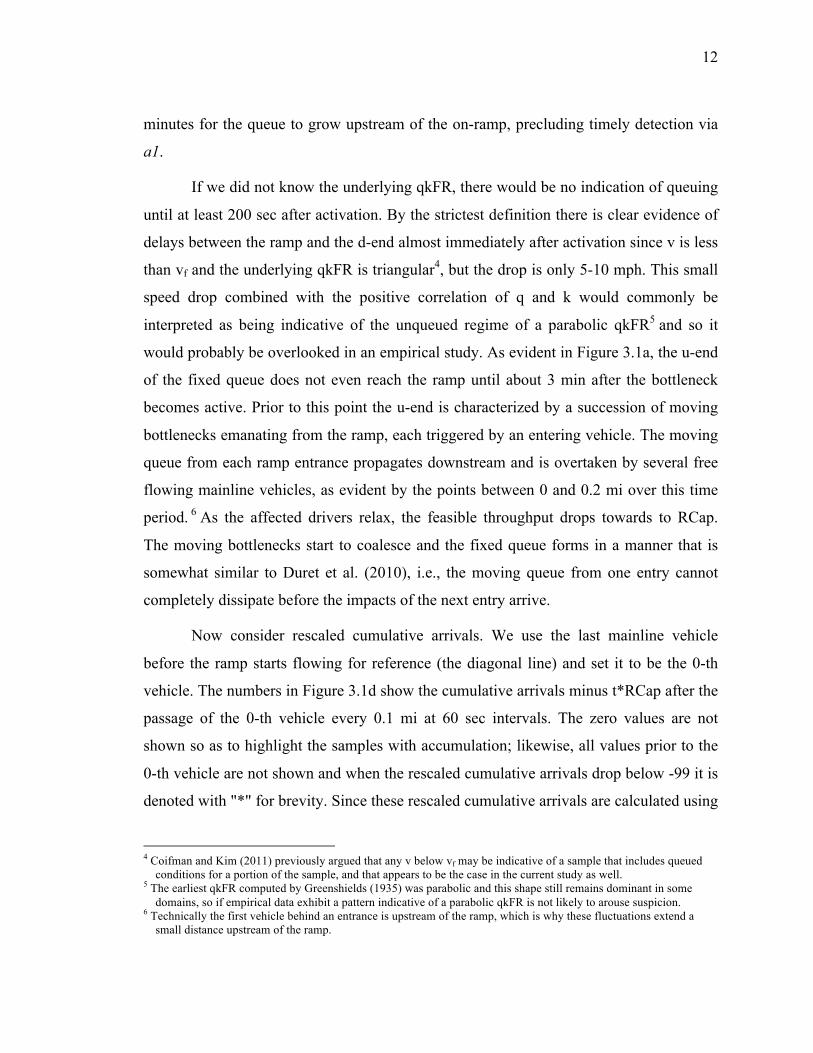
minutes for the queue to grow upstream of the on-ramp, precluding timely detection via

a1.

If we did not know the underlying qkFR, there would be no indication of queuing

until at least 200 sec after activation. By the strictest definition there is clear evidence of

delays between the ramp and the d-end almost immediately after activation since v is less

than vf and the underlying qkFR is triangular4, but the drop is only 5-10 mph. This small

speed drop combined with the positive correlation of q and k would commonly be

interpreted as being indicative of the unqueued regime of a parabolic qkFR5 and so it

would probably be overlooked in an empirical study. As evident in Figure 3.1a, the u-end

of the fixed queue does not even reach the ramp until about 3 min after the bottleneck

becomes active. Prior to this point the u-end is characterized by a succession of moving

bottlenecks emanating from the ramp, each triggered by an entering vehicle. The moving

queue from each ramp entrance propagates downstream and is overtaken by several free

flowing mainline vehicles, as evident by the points between 0 and 0.2 mi over this time

period. 6 As the affected drivers relax, the feasible throughput drops towards to RCap.

The moving bottlenecks start to coalesce and the fixed queue forms in a manner that is

somewhat similar to Duret et al. (2010), i.e., the moving queue from one entry cannot

completely dissipate before the impacts of the next entry arrive.

Now consider rescaled cumulative arrivals. We use the last mainline vehicle

before the ramp starts flowing for reference (the diagonal line) and set it to be the 0-th

vehicle. The numbers in Figure 3.1d show the cumulative arrivals minus t*RCap after the

passage of the 0-th vehicle every 0.1 mi at 60 sec intervals. The zero values are not

shown so as to highlight the samples with accumulation; likewise, all values prior to the

0-th vehicle are not shown and when the rescaled cumulative arrivals drop below -99 it is

denoted with "*" for brevity. Since these rescaled cumulative arrivals are calculated using

4 Coifman and Kim (2011) previously argued that any v below vf may be indicative of a sample that includes queued

conditions for a portion of the sample, and that appears to be the case in the current study as well. 5 The earliest qkFR computed by Greenshields (1935) was parabolic and this shape still remains dominant in some

domains, so if empirical data exhibit a pattern indicative of a parabolic qkFR is not likely to arouse suspicion. 6 Technically the first vehicle behind an entrance is upstream of the ramp, which is why these fluctuations extend a

small distance upstream of the ramp.

13

a moving time frame, the columns exhibit the same slope, vf. For example, take the fourth

column starting at the ramp and moving downstream, we see that 18 vehicles in excess of

RCap have passed 0.1 mi since the bottleneck activated, and this quantity drops to 12 veh

at 0.5 mi. Taking the difference between these two values we see an accumulation of 6

vehicles between 0.1 and 0.5 mi. Given the fact that 153 vehicles passed over this time,

even when using a3 from Section 1 it would be easy to miss this accumulation of 6

vehicles. Downstream of the ramp the rescaled cumulative arrivals are strictly non-

decreasing over time until reaching the black jagged line. This line denotes the first

instance when the rescaled cumulative arrivals decrease at the given location, and thus, q

drops below RCap for a short period before subsequently returning to RCap. The

numbers on the far right side of Figure 3.1d show the rescaled cumulative arrivals at the

given location at the end of the time window. Except for 0.1 mi, there are no more

vehicles stored downstream of the ramp. Also note that there was never any accumulation

past the d-end, but one would have to go more than 1.8 mi downstream of the ramp to

find this case over all times.

Without the driver relaxation of Section 2.3, the entire bottleneck collapses to a

point bottleneck at the on-ramp (as illustrated in Kim, 2013). The system stabilizes after a

few seconds, with the d-end remaining at the same location throughout, falling within 0.1

mi of the on-ramp from the moment the bottleneck became active (the d-end is slightly

past the on-ramp because drivers are accelerating past the point bottleneck). Queuing is

immediately evident upstream of the on-ramp, and the u-end slowly grows. In fact one

could derive the same state diagram directly using Lighthill Whitham and Richards'

macroscopic traffic flow theory (Lightthill and Whitham, 1955; Richards, 1956) with a

triangular qkFR.

3.2 Defining the loading and settling periods

Formalizing the analysis from Section 3.1, the inclusion of driver relaxation leads

to several important findings. We call the first several minutes immediately after demand

exceeds RCap the loading period. During the loading period, upstream of the on-ramp

14

there is little or no speed drop, and no evidence of queuing. Downstream of the on-ramp

q is supersaturated and in excess of RCap due to driver relaxation; however, q and k

remain positively correlated while v only drops slightly below free speed, vf. These

supersaturated conditions are actually the initial formation of the queue, storing the

demand in excess of RCap. These vehicles must be delayed while awaiting their turn to

pass the d-end, hence the slight drop in speed. Past the d-end q never exceeded RCap. In

the above example the fixed queue formed around 0.2 mi and then grew in both

directions. The d-end eventually extended more than 1.8 mi downstream of the ramp due

to the segment saturating and the relaxing drivers having to travel further before reaching

vf. The u-end took several minutes to reach the ramp, after which point, delays and

queuing first become evident upstream of the on-ramp. The loading period ends shortly

after u-end passes the on-ramp because the on-ramp vehicles enter directly into the queue

at lower speeds than before and thus, the relaxation distance shrinks. These results are

consistent with Cassidy and Bertini (1999) who found the initial queue formation 1 km

downstream of an on-ramp bottleneck.

With the shorter relaxation distance, the storage downstream of the ramp

collapses and the d-end recedes back to about 0.4 miles downstream of the on-ramp. We

refer to this interval as the settling period. During the settling period q between the ramp

and the d-end drops below RCap for a few minutes while the excess vehicles that were

stored further downstream dissipate at RCap, consuming capacity that would otherwise

be available at the on-ramp. 7 This dissipation manifests as an upstream moving

disturbance, within which both flow and speed drop to their lowest values for the given

location. The settling period ends when flow downstream of the ramp recovers to RCap.

After the settling period, the d-end stabilizes, as does the bottleneck process overall for

this case with uniform arrivals, e.g., speeds within the queue are roughly constant after

the settling period. Of course the u-end continues to grow upstream, storing the demand

in excess of capacity.

7 After a period of q above RCap, this drop below RCap should not be surprising since the long-term average q cannot

exceed RCap.

15

3.3 Alternative scenarios

Figure 3.2 repeats the simulation from Figure 3.1a for all nine scenarios listed in

Table 3.1, with uniform ramp arrivals. Comparing these nine plots, it should be clear that

the shape of the queue depends on the combination of demands from the ramp and the

mainline. For the three cases where the combined demand remains at or below RCap:

Figures 3.2a, b, and d; no fixed queue forms, one only sees evidence of moving

bottlenecks that quickly dissipate after each entrance. These moving bottlenecks are

similar to those seen during the earliest part of the loading period for the u-end in Section

3.1, except demand is not high enough for the individual disturbances to coalesce into a

fixed queue.

In the remaining six plots a fixed queue forms, the darker shading shows reduced

speeds downstream and upstream of the on-ramp. For the three queued cases with

mainline demand below RCap, Figures 3.2c, e, and f, the first 10-30 sec after demand

first exceeds capacity are seemingly indistinguishable from the moving bottlenecks of the

three cases in which no fixed queue formed. For the next 150 to 300 sec the fixed queue

remains exclusively downstream of the on-ramp, with the only sign of delay at the on-

ramp being the moving bottlenecks emanating downstream from the entering vehicles. As

in Section 3.1, within the fixed queue the supersaturated q is above RCap, but past the d-

end, q does not exceed RCap. Speeds remain above 50 mph during the loading period,

making this queuing very difficult to detect empirically. For the three cases with mainline

demand at RCap, Figures 3.2g, h, and i, the very first entering vehicle causes a fixed

queue to propagate upstream of the ramp, rather than the downstream moving bottlenecks

seen in the other six plots. As a result, there is virtually no loading period in these plots.

Finally, in all nine plots the system stabilizes by the end of the first 1,300 sec.

3.4 Stochastic ramp arrivals

Figure 3.3 repeats the same nine scenarios from Figure 3.2 using stochastic times

between individual ramp arrivals, though the ramp arrivals still have an average flow

equal to the respective column in Table 3.1. Only one set of stochastic arrivals was

16

generated for a given ramp flow and then applied to all three mainline demands to

generate a column in this figure. The basic findings from Section 3.1 remain, but the

stochasticity from the ramp introduces noise that permeates the entire bottleneck process.

The most notable difference from Figure 3.2 is in plots b and d, where the combined

demand is exactly RCap, in Figure 3.3 a standing queue forms in both cases, complete

with a loading and settling period. The queue grows when the short term demand exceeds

RCap, but when demand falls below RCap, the excess capacity can only be used if there

is already a queue, resulting in a standing queue. Unlike plots c, and e-i, the u-end does

not grow indefinitely, it stops growing after 0.5-2 miles and then fluctuates, as illustrated

in Figure 3.4a. Across the six cases with queuing in Figure 3.2, the duration of the

loading and settling periods differ in Figure 3.3 due to the short-term ramp flow

fluctuations (e.g., the loading period in Figure 3.3e is now shorter than in Figure 3.3f

even though the latter has larger combined demand). Rather than stabilizing after the

initial settling period, in Figure 3.3 the queues continue to cycle through smaller loading

and settling periods in response to the fluctuating ramp demand. As result, one now sees

upstream moving disturbances and the d-end fluctuating after the initial settling period, as

illustrated in Figure 3.4b, showing a larger portion of the data from Figure 3.3f.

Compared to Figure 3.2, the moving bottlenecks are less pronounced during the early

portion of the loading period in Figures 3.3c, e, and f.

3.5 Model calibration and other models

There are two entering vehicle parameters in the relaxation model: dcc and dv.

Lacking calibration data, we repeated the analysis in this section using several values for

these parameters. The general relationships from Section 3.2 remain, though the

relaxation distance increases as the magnitude of dcc decreases (lower deceleration rate-

less responsive) or dv decreases (entering at higher speed- requiring greater response). As

a result, the d-end and u-end both move downstream, and the duration of the loading and

settling periods increase. The reverse is true for increased dcc or dv. The magnitude of w

used in this section is typical of empirically observed values (e.g., Coifman and Wang,

2005). We have evaluated the results using a range of w and here too, the general

17

relationships presented in Section 3.2 hold over the entire range. As the magnitude of w

increases, queuing shrinks and generally both the loading and settling periods have a

shorter duration due to quicker driver response8.

Obviously the results presented herein should depend on the choice of the car

following model. Newell’s car following model is a linear form of the commonly used

GM car following model (e.g., Chandler et al., 1958; Herman et al., 1958; Herman and

Potts, 1959; Gazis et al., 1959; Gazis et al., 1961). We repeated the analysis from Section

3.1 after replacing Newell’s car following model with the model from Gazis et al. (1959),

and separately Ozaki (1993) while retaining the driver relaxation process from Section

2.3. Both of these car following models are non-linear variants of the GM models. Details

of these results are illustrated in Kim (2013). Although the shape of the queue changes

slightly, the general trends remain unchanged with a clear loading and settling period

characterized by initial queue formation downstream of the on-ramp, high v and

supersaturated q during the loading period, q drops below RCap during the settling period

and finally the traffic state stabilizes after the d-end receded upstream towards the on-

ramp.

As noted earlier, the present work seeks to use the simplest model to illustrate the

impacts of driver relaxation. However, given the potential calibration issues with our

model, we also implemented the analysis using the more complicated car following

model from Laval and Leclercq (2008) that was developed to account for lane change

maneuvers within a queue and incorporates driver relaxation. Figure 3.5a-c shows the

results for mainline demand of 2,080 vph and uniform ramp arrivals (compare to Figure

3.2d-f). While Figure 3.5d-f show the corresponding results for stochastic ramp arrivals

(compare to Figure 3.3d-f). The basic results were similar to those from our relaxation

process, as follows. Using Laval and Leclercq, when the mainline demand was below

RCap and the combined demand exceeded RCap we saw supersaturated states with q

above RCap downstream of the on-ramp. Queues were not evident upstream of the on-

ramp until several minutes after demand exceeded capacity (i.e., until after the loading

8 See Kim (2013) for more details on the evolution with different settings

18

period), in the interim, v remained at or close to vf throughout the study area (as with our

relaxation model, the traffic states looked as if they came from the unqueued regime of a

parabolic qkFR). The extent of the affected region differed slightly when using Laval and

Leclercq's model- typically it only reached a mile downstream of the on-ramp during

loading, but the d-end stayed further downstream during the settling period and beyond.

The behavior with uniform ramp arrivals once queuing set in from Laval and Leclercq

was slightly different than our model. Our model results in a single loading period and

single settling period before stabilizing at RCap. Laval and Leclercq's relaxation process

leads to a damped oscillation that cycles through loading and settling several times before

stabilizing at RCap. In any event, both models provide evidence suggesting that q

exceeds RCap during the loading period and this supersaturated q lasts for several

minutes with only subtle indications that the queue has started forming.

19

Table 3.1. Combined demand from mainline and ramp flow.

Ramp flow Mainline flow 120 vph 240 vph 360 vph

1,960 vph 2,080 vph 2,200 vph 2,320 vph 2,080 vph 2,200 vph 2,320 vph 2,440 vph 2,200 vph 2,320 vph 2,420 vph 2,540 vph

20

Figure 3.1, continued next page

21

continued from previous page

Figure 3.1. (a) Time-space plot of mainline speed (mph) with uniform ramp entrances

with mainline demand = 2,080 vph and ramp demand = 360 vph. Diagonal line shows

last vehicle past before ramp turns on, the collection of points show the u-end and d-end.

Along with the corresponding (b) flow (vph), (c) calculated density (vpm), and (d)

rescaled cumulative arrivals after the ramp turns on (zero values omitted for clarity). The

dark area in (d) shows the region with speeds below 50 mph and the jagged solid line is

the boundary between the loading and settling periods.

22

Figure 3.2. Time-space plots of mainline speed (mph) with uniform ramp entrances,

corresponding to the 9 demand combinations from Table 3.1. So the mainline demand in

row 1 is 1,960 vph, in row 2 is 2,080 vph, and in row 3 is at RCap, 2,200 vph. The ramp

demand increases from left to right. Traffic flows from bottom to top, with the ramp at

mile zero. The ramp turns on at t=0, after the mainline has loaded.

23

Figure 3.3. Time-space plots of mainline speed (mph) with stochastic ramp entrances,

corresponding to the 9 demand combinations in Table 3.1. Compare to Figure 3.2.

24

Figure 3.4. (a) d-end and u-end associated with Figures 3.3b and 3.3d over an extended

period, (b) Figure 3.3f re-plotted over a larger time range.

25

Figure 3.5. Time-space plots of mainline speed (mph) with uniform (a-c) and stochastic

(d-f) ramp entrances, corresponding to the middle row Table 3.1 using the model from

Laval and Leclercq (2008)

26

CHAPTER 4. DISCUSSION

Empirical bottleneck studies have to simultaneously deduce the bottleneck

capacity, identify the instant that the bottleneck becomes active, and where the bottleneck

actually forms. Furthermore, the low number of conventional vehicle detectors typically

precludes detailed spatial information. The detector stations used in an empirical study

could be over a mile apart. As shown in Section 3, queuing during the loading period

occurred further downstream than conventionally thought and the impacts are diffused

over such a large distance that it is very difficult to detect the early queuing.

There are many commonly held biases that make it that much more difficult to

recognize the faint evidence of queue formation during the loading period. First, the

supersaturated loading period data seemingly come from the unqueued regime of a

parabolic qkFR even though in this case the underlying qkFR was triangular. Second, the

commonly used point bottleneck model simply does not apply to the underlying

bottleneck mechanism. With driver relaxation, the bottleneck process is extended over

space. Drivers pass the on-ramp at flows above RCap and are subject to delays further

downstream, but these delays arise because drivers cannot sustain the short headways

exhibited immediately after an entrance from the on-ramp. In the remainder of this

section we discuss the specific impacts of these findings on empirical studies of

bottlenecks and the FR. At the end of this section we briefly discuss the impacts of

simulating more realistic scenarios.

4.1 Bottleneck capacity

To gain insight into empirical studies of bottleneck capacity, the three columns of

Figure 4.1 respectively show the time series detector data that would be measured 0.1,

27

0.2, and 0.6 miles downstream of the on-ramp using the data underlying the uniform

arrival scenario in Figure 3.1 and corresponding stochastic arrival scenario in Figure 3.3f.

Each plot in Figure 4.1 has one curve for the uniform ramp arrivals (via Figure 3.1) and

another curve for the stochastic ramp arrivals (via Figure 3.3f). The top row of Figure 4.1

shows the rescaled cumulative arrival curve from the individual vehicle arrivals after

subtracting a background flow equal to RCap, 2,200 vph (see, e.g., Cassidy and

Windover, 1995). Typically one does not know RCap a priori and some other convenient

background flow is used. However, in this case we do know RCap and use it as the

background flow to highlight the boundary when flow is above or below RCap. So in

Figure 4.1a the resulting curve from this background subtraction technique will be

horizontal when q is equal to the background flow. The middle row shows the time series

q for the given location using the same time axis as the top row (recall that q is the

derivative of the cumulative arrivals). Unlike Figures 3.1 and 3.3f, we use a conventional

30 sec sampling period for the moving average in Figure 4.1, and thus, some aliasing is

evident in the middle row after 800 sec, where the measured flow fluctuates about RCap.

This aliasing arises because RCap falls between resolvable values of flow and thus the

samples include a non-integer number of headways, i.e., it reflects the limitations of

sampling rather than an actual instability.9 As can be seen in the top row, the flow is

actually at RCap after 800 sec. The bottom row shows the 30 sec space mean speed at the

given location, again using the same time axis as the top row.

Now consider these measurements in the context of the so-called capacity drop if

we did not know RCap a priori. Many researchers have empirically observed the highest

q through a bottleneck just prior to the assumed activation. This high q is commonly

taken to be the bottleneck's capacity. Once the bottleneck becomes active in the reported

studies, q drops from the assumed capacity by 1% to 18% (Banks, 1991; Cassidy and

Bertini, 1999; Hall and Agyemang-Duah, 1991; Hall and Hall, 1990; Persaud and Hurdle,

1991; Zhang and Levinson, 2004, Chung et al., 2007). Most of these studies rely on either

9 This aliasing is another confounding factor that is often overlooked in the empirical studies. Care must be taken to

control for these sampling issues (e.g., by using the background subtraction technique of Cassidy and Windover, 1995), otherwise, the unbiased measurement error could be as much as 120 vph for a 30 sec sample.

28

on q or cumulative arrival curves to reach this conclusion. Unfortunately, most of these

studies also employ the conventional point bottleneck model to determine when the

subject bottleneck becomes active. Recall from Section 3 that there is no sign of queuing

or delay upstream of the on-ramp during the loading period. A conventional point

bottleneck model would not indicate that the bottleneck was active until queuing and

delays are observed upstream, i.e., sometime after the settling period has begun. By this

instant demand has exceeded capacity for some time- at least 300 sec after the bottleneck

actually activated in the case of Figure 4.1. Meanwhile, the supersaturated q downstream

of the ramp during the loading period superficially appears to be unqueued due to the fact

that the drop in speed is so small and the relationship between q and k are consistent with

a parabolic qkFR. Even if one constructed a queuing diagram to catch delays between

detectors like Cassidy and Bertini (1999), as noted in Section 3.1, the amount of

accumulation is so small that it would be hard to detect. As a result, there is no clear

indicator in the empirical data that these unsustainably high flows are in fact transient.

With the benefit of knowing RCap, return to the top row of Figure 4.1; a clear

pattern is evident at all three locations regardless of whether uniform or stochastic

arrivals on the ramp. Prior to t=0 there is no ramp flow, so the combined demand is

below RCap and the slope is negative. When the ramp begins flowing at 360 vph, the

combined demand exceeds RCap (positive slope), but the excess vehicles are being

stored further downstream, so even at mile 0.6 we see a supersaturated q in excess of

RCap. After the settling period begins, the d-end recedes upstream and many of the

vehicles stored downstream of the on-ramp dissipate, consuming some of the RCap that

would otherwise be available at the given location. So q drops below RCap (negative

slope) during the settling period. Then q stabilizes at RCap (zero slope). What's more, the

net accumulation after the settling period appears to be very small since the rescaled

cumulative arrival curve returns to almost the same value it had when the on-ramp

demand first arrived at the given location. The magnitude of the loading period

displacement decreases the further downstream one looks, reflecting the fact that vehicles

are being stored throughout the segment between the on-ramp and the d-end.

29

In the very likely scenario where one fails to recognize that the bottleneck

activates at t=0 in an empirical study, the high q of the loading period will erroneously be

assumed to be capacity leading to an overestimate of capacity. In reality the q above

RCap is simply indicative of the vehicle accumulation between the on-ramp and the d-

end, but that is very hard to detect in an empirical study. Then when the q drops at the

start of the settling period and the active bottleneck is finally detected, of course it would

look like there is a drop from capacity. On the other hand, if one were somehow able to

properly assign the activation time to t=0, when the supersaturated flow drops around 300

sec, we actually see a drop to capacity, i.e., RCap.

The true BCap cannot exceed RCap even though one should expect to measure

sustained q in excess of RCap at some locations. To avoid the impacts of the loading

period one can go beyond the d-end to measure the bottleneck's capacity, but the d-end

can extend over 1.8 miles downstream of the on-ramp. Unfortunately it is quite rare for a

bottleneck to be that isolated; often the impacts of one geometrical or operational feature

collide with the next. For example, in studying an on-ramp bottleneck Cassidy and

Rudjanakanoknad (2005) found capacity dropped due to lane change maneuvers

immediately downstream of the on-ramp.

The fact that q is at its lowest during the settling period is particularly noteworthy.

Several empirical studies show similar trends, with q dropping to its lowest value

immediately after bottleneck activation is detected and then subsequently recovering to a

higher value. In the context of Figure 4.1, this trend may be indicative of the empirical

study location actually being upstream of the d-end for a portion of time. Examples

include Persaud et al. (1998) [their Figure 1 between 75-87 min] and Cassidy and Bertini

(1999) [their Figure 5 between 6:30-6:37]. In fact Cassidy and Bertini also found cyclical

surges with a frequency comparable to those in our Figure 3.4b. Careful inspection of

their Figure 2 appears to show accumulation of about 10 vehicles on a segment thought to

be downstream of the bottleneck process, several minutes prior to the reported bottleneck

activation time. This accumulation is similar to the accumulation of 6 vehicles that we

see during the loading period in Figure 3.1d, over the same distance downstream of the

30

on-ramp. If so, then the high q observed before breakdown in these studies may actually

be supersaturated q from the loading period. However, these similarities may also simply

be by chance, since the empirical studies include many other factors not found in our

study, e.g., lane change maneuvers as per Cassidy and Rudjanakanoknad (2005). In any

event, these ambiguities highlight the need for microscopic empirical data collected at the

right locations to tease out the individual contributing factors and the present study

underscores the fact that such data collection may have to cover several miles.

4.2 The fundamental relationship

The FR is the foundation for much of traffic flow theory, yet over the past several

decades debate continues about the shape of the FR.10 Most FR's were derived from

empirical data and in this section we consider the impacts of the supersaturated states on

the observed FR. Out of convenience the discussion focuses on the qkFR.11 Once more

using the trajectories underlying Figure 3.2f with uniform ramp arrivals, Figure 4.2

shows the observed flow versus density at the three locations used in Figure 4.1. The top

row uses a 30 sec moving average and the bottom row uses a 60 sec moving average.

Recall that the underlying qkFR is triangular with vf = 60 mph, RCap = 2,200 vph, and w

= -12 mph (shown with dashed lines in the plots), yet the measured q climbs more than

10% above RCap due to the supersaturated states. If one strictly used the recorded data,

the unqueued regime of the qkFR appears to trace out a straight line with slope vf from

the origin to RCap (following the underlying triangular qkFR). Then as the

supersaturated q increases above RCap to the "apparent capacity" (i.e., the maximum

supersaturated q erroneously taken as capacity, as per Section 4.1) the empirical qkFR

bends to the right, with v dropping to 50 mph. As discussed in Section 3, the flow above

RCap is actually measured within the bottleneck process and represents the fact that

vehicles are being stored downstream.

The empirical qkFR distorted by the driver relaxation process should be

reproducible as long as demands are roughly similar from day to day on the mainline and

10 See Coifman and Kim (2011) for a review of the literature. 11 The findings translate to the other two bivariate realizations of the FR via the fundamental equation.

31

ramp. So here lies a reproducible mechanism that can pull the empirical qkFR above the

underlying qkFR, i.e., shifting away from the origin. This effect can be stable in time

because the drivers entering from the on-ramp are constantly being replenished.

However, it remains transient in space, after some distance the drivers do relax to their

preferred headways, at which point the supersaturated states disappear on the one-lane

freeway. The distortion can yield a nearly complete parabolic curve over the entire

unqueued regime, making such a location superficially look attractive for empirical

study; but because the supersaturated portion of the curve arises from the relaxation

process, the resulting qkFR is not representative of most roadway segments.

When taking the measurements from Figure 4.2 in temporal order, the traffic state

progresses in a clockwise sequence, starting from near the apex of the underlying

triangular qkFR. As one would expect, the progression is cleaner in the 60 sec data, but

the story is the same in the 30 sec data. In either case, the data progresses through the

loading period yielding most of the measurements above RCap, then q remains

supersaturated but drops below RCap during the settling period. Finally, the sequence

returns to RCap with a speed at or near vf after the vehicles stored downstream

discharge.12 Without recognizing the fact that the states are supersaturated, the apparent

capacity is higher than the real capacity, and the peak q occurs after the bottleneck has

become active. This cycle yields several values of q for a given k, likely one of the

sources of the noise in empirical qkFR.

This analysis was repeated for stochastic arrivals on the ramp with very similar

results (not shown). The one key difference is that rather than stabilizing at the apex of

the underlying qkFR after the first settling period, at mile 0.1 and 0.2 the traffic state

continued to cycle through loading and settling periods with smaller displacements from

RCap than the first cycle. These smaller perturbations did not reach mile 0.6 (see, e.g.,

Figure 3.4b), and so at that location the traffic state remained at the apex of the

underlying qkFR.

12 If the location is upstream of the d-end, speeds will be slightly below vf because traffic is still accelerating at that

location, otherwise, the final state will be at the apex of the underlying qkFR.

32

One should see similar cycles below RCap at on-ramps within the queue further

upstream, contributing noise throughout the entire queued regime of an empirical qkFR.

For example, Leclercq et al. (2007) studied an on-ramp within a queue from a

downstream bottleneck and examined the impact of driver relaxation from vehicles

entering from the ramp on the q and k measurements. In the context of the present work,

their plots clearly show supersaturated states immediately downstream of the on-ramp,

though they merely referred to these points as being "nonequilibrium". Since their study

was strictly within a queue, few of the supersaturated flows were above RCap and they

did not consider the implications on an empirically measured qkFR at the bottleneck.

4.3 More realistic details

Our objective in this report is to present a very simple model that shows beyond a

doubt that driver relaxation is an important factor that could very easily have confounded

prior empirical studies. The spatio-temporal range and magnitude of the results certainly

depend on the uncalibrated model from Section 2. This omission is due to a lack of

microscopic data for calibration. So likewise, one should not depend upon the precise

values reported herein, rather, the general trends, including:

• the loading period superficially appears to be unqueued even though it actually

occurs after the bottleneck has activated,

• the initial queue formation appears to happen downstream of the on-ramp,

• the d-end can extend over a mile downstream of the on-ramp, and

• the bottleneck process appears to occur over an extended distance that is poorly

captured with the point bottleneck model.

There were many other assumptions, in this work, discussed below, that should

also be accounted for. It is our intent that future research will address these factors and

add greater precision to refine these theories. As a first step in this direction, we relaxed

one of our assumptions in Section 3.4 and used stochastic arrivals on the ramp. We found

that the results are noisier than they are for uniform arrivals. This noise permeates to the

33

entire time-space plane, but does not disrupt the basic relationships described in Section

3.2. We suspect the same would be true if we added stochastic arrivals to the mainline, an

inhomogeneous vehicle fleet, or simulated a merge lane where vehicles were allowed to

enter the freeway over a range of distances. The results without the stochastic effects

represent a best-case scenario, adding in the stochasticity, the basic findings remain, e.g.,

the long duration of the loading period where no queues are evident upstream of the on-

ramp and q downstream of the on-ramp is supersaturated. The stochasticity introduces

large fluctuations throughout the segment that make the key transitions harder to

recognize unless you know to look for them. In the present work we are trying to tease

out the subtle phenomena at the earliest stages of bottleneck activation- so we skim away

many of these distractors.

The one-lane freeway is another such simplification, excluding the possibility for

lane change maneuvers, in part so that we can highlight the impacts of driver relaxation at

an on-ramp without the confounding effects of secondary lane change maneuvers. On a

real freeway one should see several mainline drivers change lanes to avoid the on-ramp

flow and thus, carry the driver relaxation process to the inside lanes (see, e.g., Newman,

1963). While the basic process should be similar for lane change maneuvers, the impacts

become harder to track because the maneuvers are not constrained to a specific location.

Chung et al. (2007) showed that ramp metering can reduce the number of lane change

maneuvers and thus increase queue discharge flows, i.e., the maximum sustainable

throughput depends on driver behavior. In the context of Coifman and Kim (2011) the

lane change maneuvers may preclude observing the true capacity altogether (both BCap

and RCap). If the freeway segment is operating near RCap, each lane change maneuver

sends a "hole" downstream in the exited lane and a brief delay upstream in the entered

lane.13 Combined, these two waves reduce the flow everywhere on the freeway, but they

are not a reduction in RCap, instead, they simply represent a brief departure from RCap.14

13 The "hole" propagates downstream in the exited lane because that lane is already near vf and the following vehicles

cannot close the gap. The brief delay propagates upstream in the entered lane because that lane is already at RCap, so all vehicles upstream of the maneuver must be delayed by one headway for this vehicle to enter the lane.

14 Alternatively, in this context each lane change maneuver represents a transient point bottleneck that lasts only a few seconds.

34

Since the disturbances are very small (one headway of delay per maneuver) and the lane

change maneuvers are distributed over space, the impacts of these maneuvers are very

hard to isolate. Of course lane change maneuvers are also subject to driver relaxation

(e.g., Cohen, 2004; Wang and Coifman, 2008; Leclercq et al., 2007; Xuan and Coifman,

2012). So the impacts of driver relaxation that we find in the context of an on-ramp are

also likely to translate to lane change maneuvers where drivers enter the new lane at

random locations. The above discussion of lane change maneuvers in the context of

Coifman and Kim (2011) assumed instantaneous driver relaxation. If one used more

realistic driver relaxation, the delay and the associated upstream moving wave would not

start until the affected drivers began relaxing. Very similar to what we found at the on-

ramp, the supersaturated q in the entered lane would propagate downstream with the

vehicles. As the drivers relax back to normal headways, q drops, a small delay wave

forms (one headway of delay) in the entered lane at some point downstream of the lane

change maneuver location, and then propagates upstream past the lane change maneuver

location.

Our simulations also used an abrupt change when the ramp flow switches on and

the combined demand instantaneously jumps above RCap. We would expect a slower,

more continuous demand increase at a real bottleneck, which should extend the duration

of the loading period. The long-term combined average demand might not even exceed

RCap at the onset of queuing, with minor fluctuations occasionally pushing demand

above RCap, e.g., Figures 3.3b and d. Simulation also let us study networks that were not

encumbered by confounding downstream features. All of these factors that were

simplified in the present work make it that much harder to pinpoint exactly when demand

exceeds capacity in empirical studies.

While we believe the overall findings of this work are accurate, the exact form is

highly sensitive to several factors, e.g., using Laval and Leclercq (2008) in place of our

relaxation model, we found the affected range dropped by 43%. So we feel one should

resist the temptation to build detailed models until the details of the process can be

measured empirically. The objective of this report is to document the previously

35

overlooked phenomena and associated impacts, as well as motivating future research into

the nuances of these issues.

36

Figure 4.1. Time series detector measurements at three locations downstream of the on-

ramp (by column). The first row shows the cumulative arrival curve after subtracting a

background flow equal to RCap, the second row shows q, and the bottom row shows v,

all with a common time axis. Each plot shows one curve for the uniform ramp arrivals

and another for the stochastic ramp arrivals.

37

Figure 4.2. Empirically observed q-k relationships at three locations downstream of the

on-ramp, by column, when the on-ramp has uniform arrivals (a)-(c): 30 sec sampling

period; (d)-(f): 60 sec sampling period. The underlying triangular qkFR is shown with

dashed lines in each plot.

38

CHAPTER 5. CONCLUSIONS

This simulation study examined traffic behavior in the vicinity of an on-ramp

bottleneck, revisiting commonly held assumptions and uncovering systematic biases that

likely have distorted empirical studies of bottleneck formation, capacity drop, and the

fundamental relationship. We modify Newell's car following model to include the driver

relaxation process. At the macroscopic scale the traffic state for any sample containing

one or more of these relaxing vehicles will be supersaturated. So here is a reproducible

mechanism that can pull the empirical qkFR above the underlying qkFR, i.e., shifting

away from the origin, and in some cases, above RCap.

As an on-ramp bottleneck becomes active, the entering drivers are constantly

being replenished, and keep the traffic state supersaturated. After the combined demand

first exceeds capacity in our simulations, the bottleneck activation progresses through the

following steps: (1) 10-30 sec of moving bottlenecks downstream of the on-ramp,

superficially indistinguishable from high flow, non-active conditions, but the

supersaturated q is above RCap. (2) A fixed queue forms some distance downstream of

the on-ramp and eventually extends up to 1.8 miles beyond the ramp. Between the on-

ramp and d-end, the supersaturated q remains above RCap (beyond the d-end, q never

exceed RCap). (3) The u-end grows upstream, eventually reaching the on-ramp 200-300

sec after demand first exceeded capacity. (4) With the ramp drivers now entering at lower

speeds, the relaxation distance shrinks, and thus, the d-end recedes upstream. The number

of vehicles stored downstream drops, and as they dissipate, they consume some RCap

that would otherwise be available at the ramp, i.e., q drops below RCap upstream of the

d-end. (5) Finally the system stabilizes at RCap (or near RCap in the presence of

stochastic ramp arrivals). Steps 1-3 are termed the loading period and step 4 the settling

period; both of these periods exhibit supersaturated traffic states downstream of the on-

ramp, though during the settling period q is below RCap. As noted in Section 4.3, the

time scales for these events are likely to be longer in more realistic scenarios.

39

Reinterpreting many empirical studies in the context of our results, during the

loading period a conventional point bottleneck model would erroneously indicate that the

bottleneck is inactive. In fact during the loading period most of the bottleneck activity

actually occurs downstream of the on-ramp, which is inconsistent with a simple point

bottleneck model. The bottleneck process occurs over an extended distance, in excess of

1 mile. If one fails to recognize the fact that the bottleneck is already active during the

loading period, one would overestimate the bottleneck capacity due to the supersaturated

q and the recorded activation time will be too late. Only after the settling period is over

does q return to the actual bottleneck capacity, which is equal to RCap. Instead of q

dropping "from capacity", we see q drop "to capacity" from supersaturation. If proven

empirically, this finding has important implications for traffic flow theory and traffic

control, e.g., understanding the bottleneck process and applying traffic responsive ramp

metering, respectively.

We suspect these confounding effects have largely gone unnoticed due to the

ambiguity in defining exactly what constitutes "unqueued" conditions. In fact, measuring

q, k, v from our simulation results we see a seemingly parabolic qkFR more than a mile

downstream of the on-ramp due to the driver relaxation, with the parabolic portion

coming from the supersaturated states above RCap, i.e., these locations are not strictly

downstream of the bottleneck process, and v is only slightly below vf. However, as

previously argued by Coifman and Kim (2011) any v below vf may be indicative of a

sample that includes queued conditions for a portion of the sample and that appears to be

the case in the current study as well: as long as a driver is traveling below vf they are

constrained by downstream conditions. Thus, using a strict vf criteria for unqueued states

would ensure the downstream observation site was past the entire bottleneck process, but

it would also put this site at least a mile past the on-ramp in many of our simulations- a

distance that is often infeasible due to extraneous features downstream of the on-ramp

that likely impact the measurements in empirical studies.

The driver relaxation process is a confounding factor far below the resolution of

conventional macroscopic data, and empirical studies usually fail to account for it. One

40

thing is clear, however, the bottleneck process appears to occur over a much longer

distance than previously thought, with subtle influences arising miles beyond the

apparent point bottleneck location. To advance the understanding of the bottleneck

mechanisms, our community needs to devise ways to better handle multiple interacting

features rather than assuming a simple point bottleneck. Right now we are faced with the

very daunting challenge that there are few data sources with high enough resolution to

tease out the individual contributing factors and enable such advances. So the present

work is also meant to help focus future data collection in such a way that these necessary

data will be collected from the right locations, and ultimately, so that more robust models

can eventually developed. None of the existing publicly available, microscopic, empirical

traffic data sets span the necessary region (up to two miles downstream of the apparent

bottleneck).15

15 While there are a handful of publicly available empirical microscopic data, e.g., Smith (1985), Kovvali et al. (2007),

none of them span the actual bottleneck and thus, these data sets provide little insight into the problem at hand.

41

REFERENCES

Ahn, S., Cassidy, M., Laval, J., 2004. Verification of a simplified car-following theory.

Transportation Research: part B 38(5), 431-440.

Banks, J.H., 1989. Freeway speed–flow–concentration relationships: more evidence and

interpretations. Transportation Research Record No. 1225, 53–60.

Banks, J.H., 1990. Flow processes at a freeway bottleneck. Transportation Research

Record No. 1278, 20-28.

Banks, J.H., 1991. Two capacity phenomenon at freeway bottlenecks: a basic for ramp

metering?. Transportation Research Record No. 1320, 234-241.

Bertini, R.L., Leal, M.T., 2005. Empirical study of traffic features at a freeway lane drop.

Journal of Transportation Engineering 131(6), 397-407.

Cassidy, M. J., Windover, J. R., 1995. A methodology for assessing the dynamics of

freeway traffic flow. Transportation Research Record No. 1484, 73-79.

Cassidy, M.J., Bertini, R. L., 1999. Some traffic features at freeway bottlenecks.

Transportation Research: Part B 33(1), 25-42.

Cassidy, M.J., Rudjanakanoknad, J., 2005. Increasing the capacity of an isolated merge

by metering its on-ramp. Transportation Research: Part B 39(10), 896-913.

Chandler, R. E., Herman R., and Montroll, E. W., 1958. Traffic dynamics: studies in car

following, Operations Research, 6(2), 165-184.

Chung, K., Rudjanakanoknad, J., Cassidy, M. J., 2007. Relation between traffic density

and capacity drop at three freeway bottlenecks. Transportation Research: Part B

41(1), 82-95.

42

Cohen, S.L., 2004. Application of relaxation procedure for lane changing in microscopic

simulation models. Transportation Research Record No. 1883, 50-58.

Coifman, B., 2002. Estimating travel times and vehicle trajectories on freeways using

dual loop detectors. Transportation Research: Part A 36(4), 351-364.

Coifman, B., Krishnamurthy, S., Wang, X., 2003. Lane change maneuvers consuming

freeway capacity. Proc. of the Traffic and Granular Flow 2003 Conference,

October 3, 2003, Delft, Netherlands, 3-14.

Coifman, B., and Wang, Y., 2005. Average velocity of waves propagating through

congested freeway traffic. Proc. of The 16th International Symposium on

Transportation and Traffic Theory, July 19-21, 2005, College Park, MD. 165-179.

Coifman, B., Kim, S., 2011. Extended bottlenecks, the fundamental relationship and

capacity drop. Transportation Research: Part A 45(9), 980-991.

Daganzo, C. F., 1997. Fundamentals of transportation and traffic operations. Elsevier

Science Inc., New York.

Daamen, W., Loot, M., Hoogendoorn, Serge O., 2010. Empirical analysis of merging

behavior at freeway on-ramp. Transportation Research Record No. 2188, 108-118.

Duret, A., Bouffier, J., Buisson, C., 2010. Onset of congestion due to low speed merging

maneuvers within a free-flow traffic stream: analytical solution. Transportation

Research Record No. 2188, 96-107.

Gazis, D. C., Herman, R. and Potts, R. B., 1959. Car following theory of steady state

traffic flow. Operations Research, 7(4), 499-505.

Gazis, D. C., Herman, R. and Rothery, R. W., 1961. Nonlinear follow the leader models

of traffic flow, Operations Research, 9(4), 545-567.

Greenshields, B., 1935. A study of traffic capacity. Highway Research Board Proc. 14,

448-477.

Hall, F.L., Allen, B.L., Gunter, M.A., 1986. Empirical analysis of freeway flow–density

relationships. Transportation Research: Part A 20(3), 197–210.

Hall, F.L., Agyemang-Duah, K., 1991. Freeway capacity drop and the definition of

capacity. Transportation Research Record No. 1320, 91-98.

43

Hall, F.L., Hall L,M., 1990. Capacity and speed-flow analysis of the Queen Elizabeth

way in Ontario. Transportation Research Record No. 1287, 108-118.

Hall, F. L., Hurdle, V.F., Banks, J.H., 1992. Synthesis of recent work on the nature of

speed-flow and flow-occupancy (or density) relationships on freeways.

Transportation Research Record No. 1365, 12-18.

Herman, R., Montroll, E. W., Potts, R. B. and Rothery, R. W., 1958. Traffic dynamics:

analysis of stability in car following, Operations Research, 7(1), 86-106.

Herman, R., Potts, R. B., 1959. Single Lane Traffic Theory and Experiment, Proceedings

Symposium on Theory of Traffic Flow, pp. 120-146.

Hurdle, V.F., Datta, P. K., 1983. Speeds and flows on an urban freeway: some

measurements and a hypothesis. Transportation Research Record No. 905, 127-

137.

Kim, S., (2013) Freeway on-ramp bottleneck activation, capacity, and the fundamental

relationship. PhD dissertation, the Ohio State University.

Kovvali, V., Alexiadis, V., Zhang, L., 2007. Video-based vehicle trajectory data

collection. Proc. of the 86th Annual TRB Meeting, TRB.

Laval, J.A., Daganzo, C.F., 2006. Lane-changing in traffic streams. Transportation

Research: Part B 40(3), 251-64.

Laval, J.A., and Leclercq, L., 2008. Microscopic modeling of the relaxation phenomenon

using a macroscopic lane-changing model. Transportation Research: Part B 42(6),

511-522.

Leclercq, L., Chiabaut, N., Laval, J., Buisson, C., 2007. Relaxation phenomenon after

lane changing: experimental validation with NGSIM data set. Transportation

Research Record No. 1999, 79-85.

Leclercq, L., Laval, J., Chiabaut, N., 2011. Capacity drops at merges: an endogenous

model. Transportation Research: Part B 45(9), 1302-1313.

Lighthill, M.J., Whitham, J. B., 1955. On kinematic waves. I. Flow movement in long

rivers. II. A Theory of traffic flow on long crowded roads. Proc. of Royal Soc.,

A229, 281-345.

44

Munjal, P.K., Hsu, Y.S., Lawrence, R.L., 1971. Analysis and validation of lane-drop

effects on multi-lane freeways. Transportation Research, 5(4), 257–266.

Newell, G. F., 2002. A simplified car-following theory: a lower order model.

Transportation Research: Part B 36(3), 195–205.

Newman, L., 1963. Traffic operation at two interchanges in California. Highway

Research Record No. 27, 14-43.

Ozaki, H., 1993. Reaction and anticipation in the car-following behavior. Proc. of the

12th International Symposium on Transportation and Traffic Theory, 349-362.

Persaud, B.N., Hurdle , V. F., 1991. Freeway capacity: definition and measurement

issues. Proc. of the International Symposium on Highway Capacity, Germany, 289-

307.

Persaud, B., Yagar, S., Brownlee, R., 1998. Exploration of the breakdown phenomenon

in freeway traffic. Transportation Research Record No. 1634, 64-69.

Richards, P. I., 1956. Shockwaves on the highway. Operation Research, 4, 42-51.

Smith, S.A., 1985. Freeway data collection for studying vehicle interaction. Technical

Report FHWA/RD-85/108, FHWA, USDOT.

Wang, C., Coifman, B., 2008. The effect of lane change maneuvers on a simplified car-

following theory. IEEE Transactions on Intelligent Transportation Systems, 9(3),

523-535.

Xuan, Y., Coifman, B., 2012. Identifying lane change maneuvers with probe vehicle data

and an observed asymmetry in driver accommodation. ASCE Journal of

Transportation Engineering, 138(8), 1051-1061.

Zhang, L., and Levinson, D., 2004. Some properties of flows at freeway bottlenecks.

Transportation Research Record No. 1883, 122-131.