Traditional theories of integration such as the optimum

econstorMake Your Publications Visible.

A Service of

zbwLeibniz-InformationszentrumWirtschaftLeibniz Information Centrefor Economics

Beine, Michel; Bourgeon, Pauline; Bricongne, Jean-Charles

Working Paper

Aggregate Fluctuations and International Migration

CESifo Working Paper, No. 4379

Provided in Cooperation with:Ifo Institute – Leibniz Institute for Economic Research at the University of Munich

Suggested Citation: Beine, Michel; Bourgeon, Pauline; Bricongne, Jean-Charles (2013) :Aggregate Fluctuations and International Migration, CESifo Working Paper, No. 4379, Center forEconomic Studies and ifo Institute (CESifo), Munich

This Version is available at:http://hdl.handle.net/10419/84177

Standard-Nutzungsbedingungen:

Die Dokumente auf EconStor dürfen zu eigenen wissenschaftlichenZwecken und zum Privatgebrauch gespeichert und kopiert werden.

Sie dürfen die Dokumente nicht für öffentliche oder kommerzielleZwecke vervielfältigen, öffentlich ausstellen, öffentlich zugänglichmachen, vertreiben oder anderweitig nutzen.

Sofern die Verfasser die Dokumente unter Open-Content-Lizenzen(insbesondere CC-Lizenzen) zur Verfügung gestellt haben sollten,gelten abweichend von diesen Nutzungsbedingungen die in der dortgenannten Lizenz gewährten Nutzungsrechte.

Terms of use:

Documents in EconStor may be saved and copied for yourpersonal and scholarly purposes.

You are not to copy documents for public or commercialpurposes, to exhibit the documents publicly, to make thempublicly available on the internet, or to distribute or otherwiseuse the documents in public.

If the documents have been made available under an OpenContent Licence (especially Creative Commons Licences), youmay exercise further usage rights as specified in the indicatedlicence.

www.econstor.eu


Michel Beine Pauline Bourgeon

Jean-Charles Bricongne

CESIFO WORKING PAPER NO. 4379 CATEGORY 4: LABOUR MARKETS

AUGUST 2013

An electronic version of the paper may be downloaded • from the SSRN website: www.SSRN.com • from the RePEc website: www.RePEc.org

• from the CESifo website: Twww.CESifo-group.org/wp T

http://www.ssrn.com/

http://www.repec.org/

http://www.cesifo-group.de/

CESifo Working Paper No. 4379


Abstract

Traditional theories of integration such as the optimum currency area approach attribute a prominent role to international labour mobility in coping with relative economic fluctuations between countries. However, recent studies on international migration have overlooked the role of short-run factors in explaining international migration flows. This paper aims to fill that gap. We first derive a model of optimal migration choice based on an extension of the traditional Random Utility Model. Our model predicts that an improvement in the economic activity in a potential destination country relative to any origin country may trigger some additional migration flows on top of the impact exerted by long-run factors such as the wage differential or the bilateral distance. Compiling a dataset with annual gross migration flows between 30 developed origin and destination countries over the 1980-2010 period, we empirically test the magnitude of the effect of short-run factors on bilateral flows. Our econometric results indicate that relative aggregate fluctuations and employment rates affect the intensity of bilateral migration flows. We also provide compelling evidence that the Schengen agreements and the introduction of the euro significantly raised the international mobility of workers between the member countries.

JEL-Code: F220, O150.

Keywords: international migration, business cycles, OECD countries, income maximization.

Michel Beine

CREA / University of Luxembourg [email protected]

Pauline Bourgeon

Bank of France & Paris University 1 [email protected]

Jean-Charles Bricongne

Bank of France [email protected]

This version: August 2013 This paper has benefitted from comments from the audience at various seminars held in Paris at Banque de France (internal seminar and CEPR Global Spillovers and Business Cycles conference), Moscow (HSE), Paris (Paris 1 Macro Workshop), Aix (AFSE conference). We thank in particular Simone Bertoli, Jean-François Carpantier, Xavier Chojnicki, Nicolas Coeurdacier, Frédéric Docquier, Lionel Fontagné, Jean Imbs, Daniel Mirza, Henri Pagès, Chris Parsons, Gilles Saint-Paul, Wessel Vermeulen for helpful comments on a previous version. The help of Jean-Marc Thomassin is gratefully ackowledged.

1 Introduction

International movements of workers between OECD countries have steadily increased over thelast 50 years. According to OECD data, this trend clearly intensified as of the early 1980s.1Historically, migration has always been a labor market alternative for economic agents. Inthe face of adverse economic developments, households or workers may choose to migrate toa particular external country (from a set of alternative destinations) based on considerationsthat are essentially related to expectations regarding future income. Such decisions are gen-erally based on their perceptions of current and future economic conditions both within theircountry of origin and in a number of potential destinations. Although many other factors arerelevant for migration decisions, this paper focuses on the role of short-run economic factorsin shaping the migration choice, and in particular on the role of business cycle fluctuationsand employment prospects.For many years, economists have considered labour mobility as an important macroeconomicadjustment mechanism. The literature on optimum currency areas pioneered by RobertMundell in 1961, has underscored the role of labor mobility as an adjustment mechanismwithin a currency union in the face of asymmetric shocks between the participating countriesor regions. The criterion of labour mobility has been used as a key measure in assessingwhether or not a particular area represents a so-called optimum currency area. Indeed, duringthe 90s, numerous studies disqualified Europe as an optimum currency area because of its lackof labour mobility. In contrast, Blanchard and Katz (1992) argued that labour mobility couldbe seen as a dominant adjustment mechanism in reaction to transitory fluctuations in theUnited States. In the absence of reliable data on labour movements, the supporting evidencewas however obtained via an indirect analysis based on a VAR approach involving price, wageand unemployment dynamics. One of the underlying assumptions used to infer the degree oflabour mobility is that labor mobility will induce wage and employment adjustment. This is adebatable assumption in the light of recent literature on the impact of immigration on wages(Borjas et al. (1996), Card (2001), Docquier et al. (2011)). As an alternative to this indirectapproach, this paper proposes a direct analysis of the relationship between labour mobilityand business cycle fluctuations, taking advantage of new data on migration flows and buildingon recent developments in microfounded estimable gravity models. In other words, our aim isto tackle an old problem with a fresh approach.In particular, we test how international migration flows react to economic fluctuations in asample of mostly OECD countries. To do so, we build and use data of annual migration flowsbetween 30 countries over the 1980-2010 period. We also focus on the European MonetaryUnion and in particular on the impact of the Schengen agreements and the EMU itself on thedegree of labour mobility between European countries. Such an investigation might be usefulin assessing whether Europe may be more of an OCA ex-post rather than ex-ante.2 If theintegration process itself leads to a change in the sensitivity of labour mobility to asymmetricshocks, this in turn lowers the need to rely on alternative adjustment mechanisms within amonetary union.Our analysis belongs to the extensive literature on the determinants of migration. Up to now,this literature has mostly focused on long-run factors of an economic, geographic, cultural anddemographic nature.3 We build on this extensive literature and extend it by looking at the

1Cf. OECD, International Migration Outlook 2007.2Work in this area was primarily conducted in the 90s, but using different criteria. See for instance Frankel

and Rose (1998) relating trade integration to the asymmetry in business cycle fluctuations.3Since the early work of Mayda (2010), empirical literature on the determinants of migration has developed

rapidly. For instance, among many others, Chiquiar and Hanson (2005) focus on the role of education. Grogger

2

specific marginal role of short-run factors such as the business cycle and the employment rate.In doing so, we integrate the traditional impact of long-run factors identified in the previousliterature in order to isolate the specific role of the short-run variables.There is, however, a body of recent literature acknowledging the importance of short-runfactors. Coulombe (2006) empirically investigates the determinants of internal labor mobilityin Canada. He finds an important role for the wage differentials between Canadian provincesbut finds no impact from business cycle fluctuations. Simpson and Sparber (2012) disentanglethe reaction of immigrant inflows to short-run and long-run factors between American States.Other papers also consider these short-run factors in an international perspective. Mc Kenzie,Thoharrides and Yang (2010) focus on the impact of economic fluctuations in destinations onthe intensity of emigration from the Philippines. Bertoli et al. (2013b) analyze the reactionof German immigration flows to the onset of the economic crisis in Europe. We contribute tothis literature by generalizing this type of approach to a large set of origin and destinationcountries over a period including various episodes of macroeconomic fluctuations. In turn, theuse of a large pool of origin and destination countries observed over a relatively long periodgives additional flexibility in the empirical identification of the factors. One important elementis our use of relative measures of business cycle fluctuations and employment rates allowingthe capture of situations in both origin and destination countries.Our empirical strategy directly results from the derivation of a random utility model commonlyused in the literature of determinants of migration (Borjas (1987), Grogger and Hanson (2011),Beine et al. (2011)). The income maximization framework allows the capture of migrants’choices of destination from a set of alternative destinations. The traditional benchmark modelis extended to allow some role for short-run factors. In the model, business cycles and currentemployment rates exert an ultimate role on migration as they signal the evolution of futureemployment opportunities for economic agents. The theoretical equilibrium then leads to apseudo-gravity model of international migration which can be readily estimated (Anderson,(2011)).To sum up, our contribution is thus fourfold. First, we look at the importance of cyclical shocksin explaining international migration flows in a cross-country perspective. Second, we derivean empirical specification with theoretical microfoundations. Third, we compile a completedataset of annual gross bilateral flows covering a large set of countries over 1980-2010 andincluding macroeconomic indicators both at origin and at destination. Fourth, this overallframework allows us to account for short-run and long-run factors within the same model.Our results suggest that short-run economic developments (business cycles fluctuations andemployment prospects) both at origin and at destination affect the level of bilateral migrantflows on top of the long-run factors such as the wage differential. As a by-product of theempirical analysis, we also provide evidence that the Schengen agreements and the introductionof the euro significantly raised international mobility between the countries.The remainder of the paper is organized as follows. Section 2 presents the theoretical founda-tions of our empirical model. Section 3 describes in detail the data used, thereby providing anumber of stylized facts on migration flows. Section 4 outlines the econometric model(s) andpresents the main empirical results and section 5 concludes.

and Hanson (2011) look at the role of wages while Rosenzweig (2006) focuses on skill prices. Other paperssuch as Beine et al. (2011) or McKenzie and Rapoport (2010) look at the role of networks. Clark, Hatton andWilliamson (2007) investigate the role of distance in a broad sense. Beine and Parsons (2012) focus on pushfactors like climatic shocks and natural disasters. Bertoli and Fernandez-Huerta Moraga (2012) investigatethe role of bilateral migration policies.

3

2 Theoretical background: the income maximization ap-proach

Our theoretical foundation is derived from the income maximization framework, which is usedto identify the main determinants of international migration and to pin down our empiricalspecification. The income maximization approach was first introduced by Roy (1951) andBorjas (1987) and further developed by Grogger and Hanson (2011) and Beine et al. (2011).It is also directly related to the extensive literature dealing with discrete choice models initi-ated by the seminal work of McFadden (1974). This approach allows the capture of migrants’choices of destination from a set of alternative destinations. The theoretical equilibrium leadsto the use of pseudo-gravity models of international migration which can be readily estimated(on this point, see Anderson (2011)). One of the main strengths of the income maximizationapproach is its ability to generate predictions in line with the recent (macro-economic) litera-ture on international migration. By grounding our empirical specification in a theory with awell-established track record, we try to eliminate any ad-hoc specifications and to rationalizethe obtained empirical relationships. This model has been successfully applied to analysis ofthe impact of various determinants of international migration. For instance, it has been usedto capture the specific role of wage differentials (Grogger and Hanson (2011)), the significanceof social networks (Beine et al. (2011 a and b)), the "brain-drain" phenomenon (Gibson andMcKenzie, (2011)) and the impact of climatic factors (Beine and Parsons (2012)).Our model considers homogeneous agents who decide whether or not to migrate, and then theiroptimal destination in the event they should decide to move. Agents therefore maximize theirexpected utility across the full set of possible destinations which includes the home countryas well as all possible foreign countries globally. In this study, we analyze migrations amongdeveloped countries. All included countries are therefore considered as potential origin anddestination countries. Time is included and the model is estimated over a period rangingfrom 1980 onwards using annual data. In contrast with the benchmark model of RandomUtility Maximisation used by McFadden (1974), we do not assume full employment at originand destination. In the traditional model, agents do not face any uncertainty about futureemployment, so that what matters for their optimal decision is only the amplitude of wagedifferential and the level of migration costs. In a world with unemployment rates closer to 10%rather than to what can be viewed as the natural unemployment rate, this assumption maywell be too strong. We have therefore extended the traditional RUM approach and assumedthat agents will form expectations of future employment based on information provided bythe current state of the economy. This involves the current level of economic dynamism (here,the business cycle) and the current employment rate.

2.1 Utility, income, unemployment and expectations

An individual’s utility is log-linear in expected income (E(yi,t)) and depends on the charac-teristics of his country of residence, the characteristics of any particular destination amongthe set of potential destinations, and the costs of moving between the origin and the selecteddestination.4 The utility of an individual born in country i and staying in country i at time t

4The assumption of a log-linear utility function is discussed in Anderson (2011). Note that in contrast withutility linear in income, the log-linear utility implies constant relative risk aversion (with a degree of relativerisk aversion equal to 1). Endogeneizing the wages, Anderson (2011) derives a pseudo-gravity model includinginward and outward multilateral resistance for a degree of relative risk aversion equal to 2.

4

is given by:uii,t = ln(E(yi,t)) + Ai,t + εi,t (1)

where Ai,t denotes country i’s characteristics (amenities, public expenditures,social benefitsand other push or pull factors) and εi,t is a iid extreme-value distributed random term. Theutility related to migration from country i to country j at time t is given by:

uij,t = ln(E(yj,t)) + Aj,t − Cij,t(.) + εj,t (2)

where Cij,t(.) denotes the migration costs of moving from i to j at time t. In this framework,εi,t satisfies the hypothesis of the independence of irrelevant alternatives (IIA) (see McFadden,1984).5

Agents form expectations regarding the future incomes prevailing in all possible destinationsincluding their country of origin. Expected incomes in country i and country j are given by theexpected income conditional upon being employed (the average wage level) times the expectedprobability of being employed in that country. We suppose that each individual receives someunemployment benefits in his/her native country denoted by B but not abroad. For the sakeof simplicity, B is supposed to be the same across countries, across individuals and over time,i.e. Bi,t = B. For country i, expected income is given by:

E(yi,t) = E(yi,t|ei,t = 1).E(ei,t) +B.(1− E(ei,t)) = wi,t.E(ei,t) +B.(1− E(ei,t)). (3)

where ei,t = 1 if the individual is employed in country i at time t, 0 otherwise. Expectedincome under employment E(yi,t|ei,t = 1) is given by the average level wi,t. For country j, wehave:

E(yj,t) = E(yj,t|ej,t = 1).E(ej,t) = wj,t.E(ej,t). (4)We suppose that when migrating to a new country, the migrant is not immediately eligiblefor unemployment benefits. Hence we suppose that Bj,t = 0.In turn, agents form expectations regarding the probability of being employed in the future.Given that there is uncertainty about the future stance of the economy, the expected proba-bility of employment is supposed to be given by a mixture of the current level of employmentin the economy and its current cyclical state. Migrants use both types of information sincethey encompass different types of information, both in terms of economic mechanisms and interms of forecast horizon of the employment rate in the country.The current employment rate is supposed to exert some signal to the migrants about thefuture rate of employment in the economy through extrapolative expectations. Migrants candirectly observe the current employment rate which provides a good prediction of the nextperiod employment rate for a given level of business cycle. The current level of employment rateintegrates to a certain extent the impact of past business cycles and some structural effect of thelabour market. The current business cycle provides some information which is more forwardlooking in terms of future employment rates. The rationale behind such a signalling processrefers to the feedback mechanisms from output changes to unemployment as captured forinstance by Okun’s law. This law relates the business cycle and future labour market tightnessat the aggregate level. Empirical literature has shown the relevance of this law in manydeveloped countries and has also documented that there are lags in the transmission of the

5This hypothesis implies a constant rate of substitution between alternative destinations. In the econometricframework which is derived from this model, deviations from the IIA hypothesis might lead to inconsistentestimators. Therefore, we check after estimation that our estimates are robust to the successive drop of thevarious destination countries included in the sample.

5

cycle to the labour market.6 While positive, the correlation between the current employmentrate and the business cycle is far from 1, reflecting the complex dynamics between the currentemployment rate and the business cycle. 7

Based on these assumptions, the expected probability of employment in country i is given by:

E(Prob(ei,t = 1)) = (1− uri,t)θ(bci,t)λ. (5)

where uri,t denotes the unemployment rate and bci,t is a business cycle indicator. This indicatormay be expressed on a 0 − 100% scale to match the metric in the employment rate. θ is aparameter capturing the importance of current employment rate for predicting unemploymentwhile λ captures the importance of business cycles in the expectation process.

2.2 Equilibrium migration rate

Let Ni,t be the size of the native population in country i at time t. When the random termfollows an iid extreme-value distribution, we can apply the results in McFadden (1974) towrite the probability that an agent born in country i will move to country j as:

Pr[uij,t = max

kuik,t

]=Nij,t

Ni,t

where Nij,t is the number of migrants in the i-j migration corridor at time t. Similarly, Nii,t

stands for the proportion of workers remaining in their country of origin during period t. Thisgives:

Nij,t

Ni,t

=exp [ln(wj,t) + θln(1− urj,t) + λln(bcj,t) + Aj,t − Cij,t]∑

k exp [ln(wk,t) + θln(1− urk,t) + (λln(bck,t) + ln(B ∗ urk,t) + Ak,t − Cik,t](6)

Likewise we may compute the equilibrium rate of stayers over natives, giving the equilibriumprobability for a native to stay in his or her own country rather than emigrating as:

Nii,t

Ni,t

=exp [ln(wi,t) + θln(1− uri,t) + (λ)ln(bci,t) + ln(B ∗ uri,t) + Ai,t]∑

k exp [ln(wk,t) + θln(1− urk,t) + (λ)ln(bck,t) + ln(B ∗ urk,t) + Ak,t − Cik,t](7)

The equilibrium bilateral migration rate between i and j is obtained by taking the ratio(Nij,t/Nii,t) at equilibrium :

Nij,t

Nii,t

=exp [ln(wj,t) + θln(1− urj,t) + (λ)ln(bcj,t) + Aj,t − Cij,t]

exp [ln(wi,t) + θln(1− uri,t) + (λ)ln(bci,t) + ln(B ∗ uri,t) + Ai,t](8)

Taking logs, we obtain an expression giving the log of the bilateral migration rate between i6Early estimates of the transmission lags in the Okun’s law amount to about 6 to 8 quarters, i.e. 1.5 to

2 years. For some recent evidence on Okun’s law in OECD countries, see among others Ball et al. (2013)Gordon (2010) and Lee (2000). In general the empirical literature points to the relevance of Okun’s law for alldeveloped countries, although with different sensitivities of unemployment rate to output fluctuation. Thereis also a general controversy on whether there has been a shift in the average key elasticity and on whetherthere are asymmetries in the response of unemployment to output shocks.

7Depending on the measure of the business cycle, the correlation between the relative employment rate andthe relative business cycle is comprised between 0.02 and 0.24.

6

and j over stayers at time t:

ln(Nij,t

Nii,t

) = ln(wj,twi,t

)+θln(1− urj,t1− uri,t

)+(λ)ln(bcj,tbci,t

)− ln(B)− ln(uri,t)+Aj,t−Ai,t−Cij,t(.) (9)

Expression (9) allows us to identify the main components of the aggregate bilateral migrationrate:(i) the wage differential in the form of the wage ratio (wj,t

wi,t), (ii) differential in employment

rates, (iii) differential in business cycles; (iv) differential in pull and push factors at destinationAj,t, and at origin (Ai,t); (v) the level of unemployment benefits in the origin country; (vi) theunemployment rate in the country of origin and (vii) finally the bilateral migration costs be-tween i and j, Cij,t. It should be emphasized that in that framework, a rise in unemploymentin the origin country exerts two separate effects. The first one is that in presence of unem-ployment benefits, an increase in unemployment rate might reduce the propensity to migrate.This effect is stronger the higher the average level of unemployment benefits paid to nativeworkers. If the native is not eligible for unemployment benefits or if the origin country doesnot pay benefits (B = 0), then this effect does not exist and only the second effect prevails.8Second, an increase in current unemployment lowers the probability of employment for theindividual and increases the differential with respect to the potential destinations. This favorsemigration from country i.Note that by construction, the impact of the relative business cycle on the bilateral migrationrate is proportional to its importance for building expectations of future employment rate. Thisreflects the theoretical channel that is favored in the model. Nevertheless, in the empiricalpart, the estimated value of λ could be also driven by alternative channels.

2.3 Migration costs

Putting everything together, our cost function may be expressed as:

Cij,t = c(xi, xj, xij, xit, xjt, xt, xijt) (10)

The cost function is supposed to be separable (i) into time-invariant origin country factors(xi) such as being an island, being landlocked, time-invariant destination country factors (xj)such as being an island, being landlocked (ii) country pair specific time-invariant (xij) thatinclude for instance linguistic proximity or bilateral migration policies that are constant overthe period under investigation, (iii) time-varying origin country factors (xit) that include forinstance unemployment benefits at origin or human capital level of the country, (iv) time-varying destination specific factors (xjt) such as unilateral immigration policies and finally(v) time-varying pair-specific factors xijt such as diasporas at destination or time-varyingbilateral policies between the origin and the destination, such as the Schengen agreementsin Europe. Given the data dimension, all those cost components, except one can be eitherdirectly observed or captured by the relevant combination of fixed effects. The main exceptionis of course the last component which requires only observable variables for that componentto be explicitly accounted for, otherwise, it would encompass all other variables.

8Note however that our framework does not account for liquidity constraints in the migration process. Ifunemployment at origin makes those constraints more binding, this could lead to an additional decrease in thebilateral migration flows. We do not account explicitely for such a possibility but this could be done easily bymaking the bilateral migration costs Cij,t to depend on uri,t. In that case, the estimated coefficient of uri,twill capture the joint effect due to unemployment benefits and liquidity constraints.

7

3 Data

The estimation of the equilibrium condition (9) requires the collection of data relative to inter-national migration, relative to economic outcomes such as aggregate wage, GDP, employmentrates and relative to relationships between countries such as bilateral agreements or geographicdistance.

3.1 Migration and population data

The key data needed to estimate equation (9) is about international migration. From equation(9), we can identify three important and desirable features for this data. First, the data mustcapture flows of international migration between countries. Second, the dimension must bedyadic, i.e. the data must capture flows between country pairs. Furthermore, the internationalmigration data must have a large enough time dimension. Finally, given the focus on the roleof economic fluctuations in explaining international migration flows, the migration flows mustbe observed at a business cycle frequency. To the best of knowledge, there is no ready-to-usedataset combining those desirable features.9

To estimate equation (9), we also need to know the population of native workers Nii,t. Sincethis data is not available and cannot be computed on an annual basis, we proxy it by Ni,t.This latest data of total population in a given country i at year t is obtained from the WorldPopulation Prospects (2010 revision database). This database is produced by the Popula-tion Division (Department of Economic and Social Affairs) of the United Nations. Datacover total populations (both genders combined) of major countries, on an annual basis, from1950 to 2010. The corresponding data can be found on http://esa.un.org/unpd/wpp/Excel-Data/population.htm.As a result, following number of previous authors who have studied migration flows, we builtour own dataset combining different sources of information.10 Our migration data displayimportant features in terms of cross-country coverage and in terms of time span. First, ourbilateral migration flows cover 30 origin and destination countries.11 Overall, our data capturesan important share of total international migration to and from OECD countries.12 Second,

9For instance, two well-known cross-country data on international migration, namely Docquier and Marfouk(2007) on the one hand and Ozden et al. (2011) on the other hand are suited more for capturing the long-rundeterminants of international migration. Docquier, Marfouk and Lowell (2009) provide bilateral migrationstocks with information about education levels (as well as gender) for two years only, 1990 and 2000. Ozdenet al. (2011) provide a complete coverage at the global level of bilateral stocks for 5 years (1960, 1970, 1980,1990 and 2000) by gender only.

10For instance, Belot and Ederveen (2012) build their own dataset to analyse the role of cultural barriersbetween 22 OECD countries over the 1990-2003 period. Pedersen et al. (2008) build migration flows for27 OECD countries and more than 120 origin countries for the 1990-2000 period. They combine informationprovided by the national statistical offices of the destination countries with OECD data extracted from "Trendsin International Migration".

11The list of countries is: Australia, Austria, Belgium, Canada, Croatia, Czech Republic, Denmark, Finland,France, Germany, Greece, Hungary, Iceland, Ireland, Israel, Italy, Luxembourg, the Netherlands, New Zealand,Norway, Portugal, Romania, Russia, Slovakia, Slovenia, Sweden, Switzerland, the United States, Spain andthe UK.

12Comparing our data with the most comprehensive data provided by Docquier, Marfouk and Lowell (2007),we cover most of the migration process between OECD countries. Our data does not include 6 destination

8

we capture annual migration flows over a period of 30 years, from 1980 to 2010. Our sampleperiod therefore covers a number of major episodes of economic fluctuations in the modernera, such as the recession following the second oil shock in the early 80’s, the recovery of thelate eighties in many OECD countries, the US recession in the early nineties, the Europeanrecession of the mid-nineties, the US expansion in the late nineties and last but not least thefinancial crisis in 2008.Appendix A gives the details of the collected migration data in terms of definitions, sourcesand available information.We combine two sources, the international migration flows datasetfrom the UN 13 and the OECD International Migration database.14 These two databasesgive us, for all destination countries, migrant inflows by origin country. They both aggregateinformation registered at the country level. Since the national authorities use different datacollection processes and because we associate two different sources, we face some potentialproblems of data comparability. The first one is geographic and time coverage. Only a fewcountries provide data for all origin countries over the whole period (1980-2010). In order tokeep a sufficiently balanced panel data set, we retained in our final selection only countrieswhich provided data on a substantial number of origins and over a long enough period oftime. Another issue relates to the definition of migrant flows because national authoritiesuse three distinct criteria to register immigrants. We tried to keep the same criterion for allcountries to obtain as harmonized a sample as possible. Most countries in our sample use theresidence criterion, others use the citizenship criterion and only one country uses the countryof birth criterion.15 The last issue refers to particular migrant groups. Some countries registeronly foreigners migrants and do not consider citizens who migrate back to their country oforigin.16 The residence criterion allows us to capture better short-term mobility since it coversthe last origin of migrants, while citizenship and birth criteria capture respectively long-termimmigrants and immigrants from a permanent origin. The residence criterion involves thedelivery of a residence permit, the duration of stay considered varies among countries.17 Inaddition, it is important to remember that the date of a residence permit may or may notcoincide with the date of arrival of a migrant.In spite of a strong selection of countries, our panel data set remains quite unbalanced in termsof migration flows. Overall, we have a significant number of missing observations but very fewzero values. For all years, all origins and destination countries, we have 11816 missing values,i.e. 43.8% of all potential observations. In contrast, we have only 206 zero flows, i.e. lessthan 1% of our observations. These 206 zero flows represent less than 1.5% of the non-missingobservations. In terms of econometric implications, the low occurrence of zeros allows us to usethe traditional panel data methods as opposed to the alternative techniques such as Poisson

countries (out of 31) covered by Docquier et al. (2007): Japan, Korea, Mexico, Poland, Turkey and SouthAfrica. Still, the 25 common destination countries represent respectively 90 and 91% of total migration stockscaptured in Docquier et al. (2007) respectively for 1990 and 2000; and it represents 96% of skilled migrantsobserved in 1990 and 2000. With respect to Docquier et al. (2007), we capture 4 additional destinationcountries, namely Romania, Russia, Slovakia and Croatia.

13This dataset is provided by United Nations Population division. More information may be found onhttp://www.un.org/esa/population/migration/ .

14Downloadable on http://stats.oecd.org/15For countries for which it was possible, we checked the correlation between alternative criteria. We get

quite a positive correlation in the range of 0.8.16We also checked that this, in terms of migrant definition, would not be an issue for our analysis.17More information is available on http://www.un.org/esa/population/migration/CD-

ROM%20DOCUMENTATION_UN_Mig_Flow_2010.pdf

9

Maximum likelihood or hurdle models.18

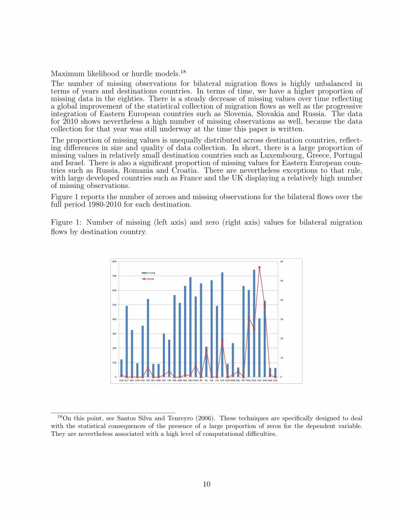
The number of missing observations for bilateral migration flows is highly unbalanced interms of years and destinations countries. In terms of time, we have a higher proportion ofmissing data in the eighties. There is a steady decrease of missing values over time reflectinga global improvement of the statistical collection of migration flows as well as the progressiveintegration of Eastern European countries such as Slovenia, Slovakia and Russia. The datafor 2010 shows nevertheless a high number of missing observations as well, because the datacollection for that year was still underway at the time this paper is written.The proportion of missing values is unequally distributed across destination countries, reflect-ing differences in size and quality of data collection. In short, there is a large proportion ofmissing values in relatively small destination countries such as Luxembourg, Greece, Portugaland Israel. There is also a significant proportion of missing values for Eastern European coun-tries such as Russia, Romania and Croatia. There are nevertheless exceptions to that rule,with large developed countries such as France and the UK displaying a relatively high numberof missing observations.Figure 1 reports the number of zeroes and missing observations for the bilateral flows over thefull period 1980-2010 for each destination.

Figure 1: Number of missing (left axis) and zero (right axis) values for bilateral migrationflows by destination country.

30

40

50

60

400

500

600

700

800

missing

zeroes

0

10

20

0

100

200

300

AUS AUT BEL CAN CHE CZE DEU DNK ESP FIN FRA GBR GRC HRV HUN IRL ISL ISR ITA LUX NLD NOR NZL PRT ROU RUS SVK SVN SWE USA

18On this point, see Santos Silva and Tenreyro (2006). These techniques are specifically designed to dealwith the statistical consequences of the presence of a large proportion of zeros for the dependent variable.They are nevertheless associated with a high level of computational difficulties.

10

3.2 Wages, business cycles, employment rates and bilateral migra-tion costs

Our key equilibrium equation (9) implies that we also need data on wages, business cycles,employment and unemployment rates at origin and destination. Many cross-country analy-ses of migration flows face issues in finding comparable measures of wages across countries.Grogger and Hanson (2011) definitely provide the best approach with respect to this issue,recovering wages by education level from the observed wage distribution in microeconomicdatabases specific to each destination country. This is made possible however by the relativelylow number of countries (only 13) considered in their analysis. Some studies capture wages byproxies such as GDP per capita, which might imply significant measurement errors in somecases. 19 Other analyses do not directly observe wage data but capture their role through theuse of fixed effects. 20

In this paper, in contrast to those previous studies, we use explicit measures of wages at originand destination (see Appendix A for more detail).We extract cyclical stance from GDP data and use two different measures. The first onerelies on the deviation from GDP trend and uses the traditional Hodrik-Prescott filter for thatpurpose. Given the annual frequency, we extract the trend based on a value of the smoothingparameter λ equal to 400. As an alternative, we use a more simple measure based on theannual growth rate of GDP. We also rely on the standardized unemployment rates providedby the OECD. These are used to build differential in employment rates and unemploymentrates at origin as identified in equation (11). The exact data sources are also provided inAppendix A.In addition to these measures, we also capture time-varying dyadic variables (xijt in termsof equation (10)) thought to affect bilateral migration costs. We use three main measures totackle integration between countries: (i) Schengen agreements between (a subset of) Europeancountries, (ii) other bilateral agreements favouring the international mobility of workers and(iii) joint membership of the European Monetary Union. These measures are explained belowin more details when discussing the benchmark econometric specification (see section 4.1.).The exact construction and sources of the bilateral agreements are also described more indetails in Appendix B.

19See for instance Beine and Parsons (2012) who capture wage differentials by differences in GDP per capitafor all origin and destination countries.

20See for instance Beine et al. (2011) and Bertoli and Fernandez-Huerta Moraga (2013a).

11

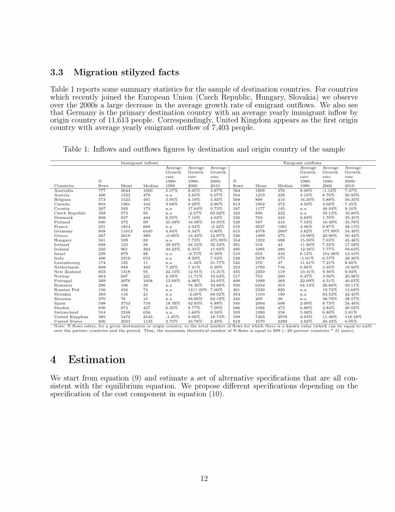
3.3 Migration stilyzed facts

Table 1 reports some summary statistics for the sample of destination countries. For countrieswhich recently joined the European Union (Czech Republic, Hungary, Slovakia) we observeover the 2000s a large decrease in the average growth rate of emigrant outflows. We also seethat Germany is the primary destination country with an average yearly immigrant inflow byorigin country of 11,613 people. Correspondingly, United Kingdom appears as the first origincountry with average yearly emigrant outflow of 7,403 people.

Table 1: Inflows and outflows figures by destination and origin country of the sample

Immigrant inflows Emigrant outflows

CountriesNflows Mean Median

AverageGrowthrate1980-1990



Nflows Mean Median




Australia 777 4644 1000 5.57% 8.65% 3.87% 564 1909 376 8.00% -1.12% 7.47%Austria 406 1322 479 n.a 3.83% 6.07% 564 1219 228 4.16% 8.70% 20.93%Belgium 573 1523 491 3.95% 4.19% 5.93% 568 899 410 16.20% 5.88% 50.35%Canada 803 1361 442 3.68% 9.29% 2.86% 614 1802 372 4.50% 4.66% 7.45%Croatia 207 393 173 n.a 17.64% 0.73% 347 1177 145 n.a 48.04% 9.10%Czech Republic 358 572 93 n.a -2.57% 69.02% 322 839 222 n.a 33.13% 16.80%Denmark 808 937 444 6.55% 7.10% 4.92% 526 763 343 6.69% 1.70% 35.45%Finland 640 372 99 35.09% 16.98% 10.95% 539 567 216 7.53% 10.49% 35.76%France 331 1854 668 n.a 4.34% -2.42% 516 3027 1361 3.06% 8.87% 48.15%Germany 808 11613 6445 4.84% 0.34% 0.80% 615 4578 2667 3.82% 177.99% 34.49%Greece 267 2019 289 -0.66% 14.43% 12.87% 520 1489 275 10.99% 20.90% 56.44%Hungary 341 509 82 n.a 7.72% 475.99% 554 1202 698 15.00% 7.62% 45.46%Iceland 688 122 28 39.92% 24.52% 35.34% 391 218 44 11.80% 7.32% 17.58%Ireland 250 961 302 34.23% 6.35% 17.83% 495 1085 280 12.56% 7.77% 59.63%Israel 229 879 88 n.a -6.75% 6.39% 510 653 216 6.12% 101.06% 13.10%Italy 406 3319 653 n.a 8.29% 7.52% 528 3478 575 -1.01% 6.57% 38.26%Luxembourg 174 125 11 n.a -1.34% 21.77% 542 270 37 11.61% 7.21% 8.60%Netherlands 808 949 402 7.26% 7.41% 6.39% 552 1760 716 0.96% 5.95% 18.56%New Zealand 833 1318 93 22.10% 12.91% 15.31% 435 2350 119 10.41% 9.56% 9.92%Norway 664 687 221 2.59% 11.71% 10.64% 517 753 260 9.47% 3.90% 20.96%Portugal 269 3076 1058 13.69% 4.98% 24.65% 499 1999 369 22.09% 4.51% 40.65%Romania 296 106 29 n.a 74.36% 33.88% 500 6334 353 64.12% 26.66% 32.11%Russian Fed. 156 434 74 n.a 1411.00% 7.00% 361 5330 920 n.a 19.73% 14.68%Slovakia 493 116 21 n.a -2.00% 68.02% 354 1104 190 n.a 63.53% 42.43%Slovenia 370 78 15 n.a 58.66% 62.19% 345 209 38 n.a 38.79% 38.57%Spain 598 3753 718 18.76% 42.83% 6.88% 540 2084 608 2.09% 8.73% 24.44%Sweden 836 972 427 6.35% 9.77% 7.99% 566 1066 473 6.86% 2.84% 30.03%Switzerland 544 2248 656 n.a 1.60% 6.59% 593 1490 358 5.00% 6.80% 5.81%United Kingdom 385 5473 2545 -1.35% 9.06% 18.74% 558 7403 2978 3.94% 11.49% 118.58%United States 836 2933 1135 3.70% 16.78% 2.49% 619 4570 2289 4.82% 40.43% 6.05%Note: N flows refers, for a given destination or origin country, to the total number of flows for which there is a known value (which can be equal to null)over the partner countries and the period. Thus, the maximum theoretical number of N flows is equal to 899 (=29 partner countries * 31 years).

4 Estimation

We start from equation (9) and estimate a set of alternative specifications that are all con-sistent with the equilibrium equation. We propose different specifications depending on thespecification of the cost component in equation (10).

12

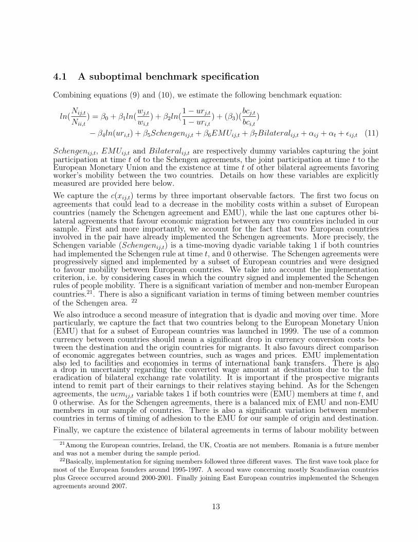
4.1 A suboptimal benchmark specification

Combining equations (9) and (10), we estimate the following benchmark equation:

ln(Nij,t

Nii,t

) = β0 + β1ln(wj,twi,t

) + β2ln(1− urj,t1− uri,t

) + (β3)(bcj,tbci,t

)

− β4ln(uri,t) + β5Schengenij,t + β6EMUij,t + β7Bilateralij,t + αij + αt + εij,t (11)

Schengenij,t, EMUij,t and Bilateralij,t are respectively dummy variables capturing the jointparticipation at time t of to the Schengen agreements, the joint participation at time t to theEuropean Monetary Union and the existence at time t of other bilateral agreements favoringworker’s mobility between the two countries. Details on how these variables are explicitlymeasured are provided here below.We capture the c(xij,t) terms by three important observable factors. The first two focus onagreements that could lead to a decrease in the mobility costs within a subset of Europeancountries (namely the Schengen agreement and EMU), while the last one captures other bi-lateral agreements that favour economic migration between any two countries included in oursample. First and more importantly, we account for the fact that two European countriesinvolved in the pair have already implemented the Schengen agreements. More precisely, theSchengen variable (Schengenij,t) is a time-moving dyadic variable taking 1 if both countrieshad implemented the Schengen rule at time t, and 0 otherwise. The Schengen agreements wereprogressively signed and implemented by a subset of European countries and were designedto favour mobility between European countries. We take into account the implementationcriterion, i.e. by considering cases in which the country signed and implemented the Schengenrules of people mobility. There is a significant variation of member and non-member Europeancountries.21. There is also a significant variation in terms of timing between member countriesof the Schengen area. 22

We also introduce a second measure of integration that is dyadic and moving over time. Moreparticularly, we capture the fact that two countries belong to the European Monetary Union(EMU) that for a subset of European countries was launched in 1999. The use of a commoncurrency between countries should mean a significant drop in currency conversion costs be-tween the destination and the origin countries for migrants. It also favours direct comparisonof economic aggregates between countries, such as wages and prices. EMU implementationalso led to facilities and economies in terms of international bank transfers. There is alsoa drop in uncertainty regarding the converted wage amount at destination due to the fulleradication of bilateral exchange rate volatility. It is important if the prospective migrantsintend to remit part of their earnings to their relatives staying behind. As for the Schengenagreements, the uemij,t variable takes 1 if both countries were (EMU) members at time t, and0 otherwise. As for the Schengen agreements, there is a balanced mix of EMU and non-EMUmembers in our sample of countries. There is also a significant variation between membercountries in terms of timing of adhesion to the EMU for our sample of origin and destination.Finally, we capture the existence of bilateral agreements in terms of labour mobility between

21Among the European countries, Ireland, the UK, Croatia are not members. Romania is a future memberand was not a member during the sample period.

22Basically, implementation for signing members followed three different waves. The first wave took place formost of the European founders around 1995-1997. A second wave concerning mostly Scandinavian countriesplus Greece occurred around 2000-2001. Finally joining East European countries implemented the Schengenagreements around 2007.

13

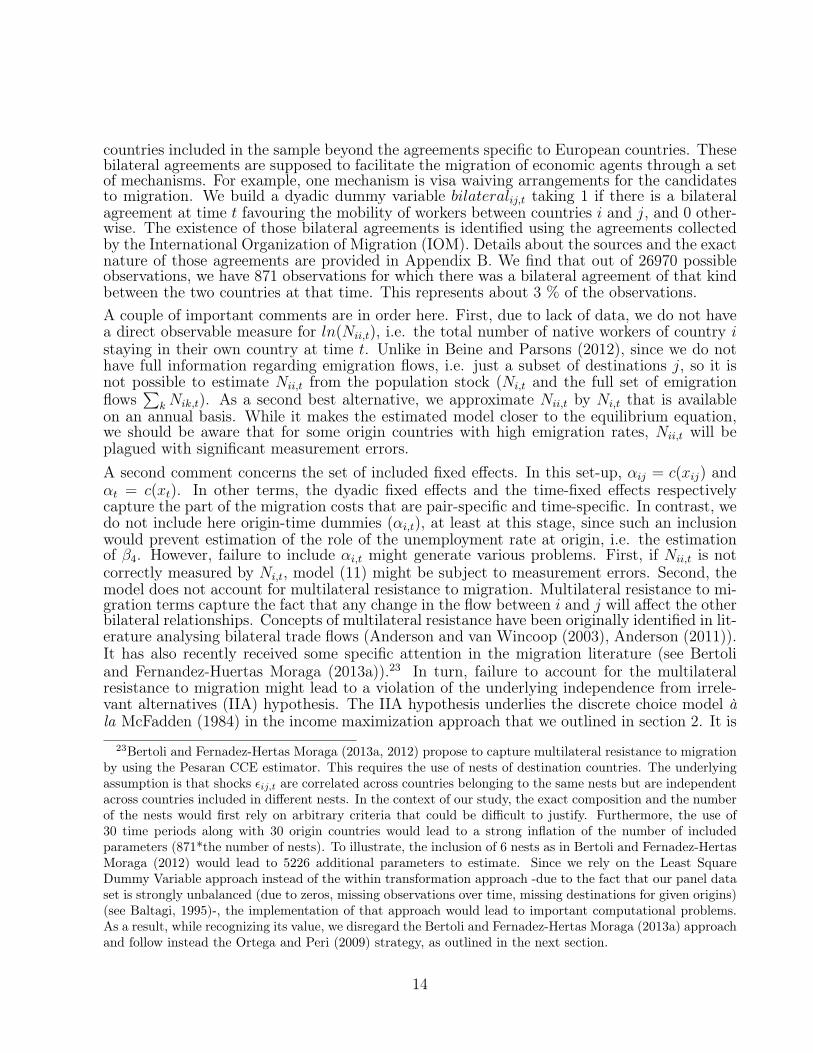
countries included in the sample beyond the agreements specific to European countries. Thesebilateral agreements are supposed to facilitate the migration of economic agents through a setof mechanisms. For example, one mechanism is visa waiving arrangements for the candidatesto migration. We build a dyadic dummy variable bilateralij,t taking 1 if there is a bilateralagreement at time t favouring the mobility of workers between countries i and j, and 0 other-wise. The existence of those bilateral agreements is identified using the agreements collectedby the International Organization of Migration (IOM). Details about the sources and the exactnature of those agreements are provided in Appendix B. We find that out of 26970 possibleobservations, we have 871 observations for which there was a bilateral agreement of that kindbetween the two countries at that time. This represents about 3 % of the observations.A couple of important comments are in order here. First, due to lack of data, we do not havea direct observable measure for ln(Nii,t), i.e. the total number of native workers of country istaying in their own country at time t. Unlike in Beine and Parsons (2012), since we do nothave full information regarding emigration flows, i.e. just a subset of destinations j, so it isnot possible to estimate Nii,t from the population stock (Ni,t and the full set of emigrationflows

∑kNik,t). As a second best alternative, we approximate Nii,t by Ni,t that is available

on an annual basis. While it makes the estimated model closer to the equilibrium equation,we should be aware that for some origin countries with high emigration rates, Nii,t will beplagued with significant measurement errors.A second comment concerns the set of included fixed effects. In this set-up, αij = c(xij) andαt = c(xt). In other terms, the dyadic fixed effects and the time-fixed effects respectivelycapture the part of the migration costs that are pair-specific and time-specific. In contrast, wedo not include here origin-time dummies (αi,t), at least at this stage, since such an inclusionwould prevent estimation of the role of the unemployment rate at origin, i.e. the estimationof β4. However, failure to include αi,t might generate various problems. First, if Nii,t is notcorrectly measured by Ni,t, model (11) might be subject to measurement errors. Second, themodel does not account for multilateral resistance to migration. Multilateral resistance to mi-gration terms capture the fact that any change in the flow between i and j will affect the otherbilateral relationships. Concepts of multilateral resistance have been originally identified in lit-erature analysing bilateral trade flows (Anderson and van Wincoop (2003), Anderson (2011)).It has also recently received some specific attention in the migration literature (see Bertoliand Fernandez-Huertas Moraga (2013a)).23 In turn, failure to account for the multilateralresistance to migration might lead to a violation of the underlying independence from irrele-vant alternatives (IIA) hypothesis. The IIA hypothesis underlies the discrete choice model àla McFadden (1984) in the income maximization approach that we outlined in section 2. It is

23Bertoli and Fernadez-Hertas Moraga (2013a, 2012) propose to capture multilateral resistance to migrationby using the Pesaran CCE estimator. This requires the use of nests of destination countries. The underlyingassumption is that shocks εij,t are correlated across countries belonging to the same nests but are independentacross countries included in different nests. In the context of our study, the exact composition and the numberof the nests would first rely on arbitrary criteria that could be difficult to justify. Furthermore, the use of30 time periods along with 30 origin countries would lead to a strong inflation of the number of includedparameters (871*the number of nests). To illustrate, the inclusion of 6 nests as in Bertoli and Fernadez-HertasMoraga (2012) would lead to 5226 additional parameters to estimate. Since we rely on the Least SquareDummy Variable approach instead of the within transformation approach -due to the fact that our panel dataset is strongly unbalanced (due to zeros, missing observations over time, missing destinations for given origins)(see Baltagi, 1995)-, the implementation of that approach would lead to important computational problems.As a result, while recognizing its value, we disregard the Bertoli and Fernadez-Hertas Moraga (2013a) approachand follow instead the Ortega and Peri (2009) strategy, as outlined in the next section.

14

therefore important to check after estimation that the IIA hypothesis holds given the adoptedspecification.These concerns shed some doubts on the validity of the estimates of model (11). This is whywe report the full results in Appendix C and give here only a quick summary of the mainresults. The main value added of model 11 is that it allows identification of the marginalimpact of unemployment at origin. Overall, the estimation results support a negative impactof unemployment on the bilateral emigration rate on top of the impact of the differential inemployment opportunities. This result is consistent with the one considered in the model. Ifunemployment benefits are only available for native workers and not for migrants (at leastshortly after arrival) and in the presence of uncertainty of being employed in the destina-tion, an increase in unemployment might reduce the propensity to emigrate. This marginalnegative impact offsets at least partly the positive impact of the differential in employmentrates between the origin and the destination, so that the net total effect of unemployment isuncertain. A second mechanism, not considered in our theoretical model, might also generatethe negative marginal impact of unemployment, namely the presence of liquidity constraints.If unemployment raises the number of people subject to liquidity constraints, this would de-crease the number of potential migrants able to cover the migration costs, which in turn wouldlead to a decrease in the emigration rates.Beyond the impact of unemployment, we find some support for the key mechanisms identifiedin equation (11). In particular, we find a positive impact of the wage differential, the businesscycle differential and employment opportunities. Results also support a significant impact ofSchengen agreements and EMU participation in terms of lowering migration costs betweencountries. Nevertheless, given the reservations mentioned above, these results should be com-pleted with other models taking into account the influence of countries other than the originand the destination countries. These models are considered in the next sections.The results in Table 6 and 7 yield some interesting insights. First, we find some support forthe key mechanisms identified in equation (11). In particular, we find a positive impact ofthe wage differential, the business cycle differential and employment opportunities. Resultsalso support a significant impact of Schengen agreements and EMU participation in terms oflowering migration costs between countries. Nevertheless, given the reservations mentionedabove, these results should be completed with other models taking into account the influenceof countries other than the origin and the destination countries. The main value added ofmodel (11) is that it allows for the identification of the marginal impact of unemployment atorigin.Nevertheless, overall those results should be treated with caution, to the extent that model(11) might suffer from mis-specification problems. By way of a straightforward illustrationthe results relative to the bilateral agreements cast some doubts on the estimation properties.The impact is found to be significantly negative while we would expect either a positive ora negligible impact. One reason might be that model (11) fails to include some multilateralresistance terms that might be correlated with the bilateral agreements. In that case, it wouldgenerate a bias in the estimation due to omitted variables. The negative elasticity obtainedin columns (1) and (5) suggests that this might be the case here. In turn, failure to integratethose terms might lead to a violation of the IIA assumption. The inclusion of time-originfixed effects αit in a slightly modified specification (see next section) will capture the outwardmultilateral resistance to migration.

15

4.2 Accounting for origin-time fixed effects

In order to take into account important elements like the outward multilateral resistance tomigration, we modify model (11) and consider an alternative specification that specificallyincludes αit fixed effects. The specification takes the following form:

ln(Nij,t) = β0 + β1(ln(wj,twi,t

)) + β2ln(1− urj,t1− uri,t

) + β3(bcj,tbci,t

) + β4Schengenij,t

+ β5EMUij,t + β6bilateralij,t[+β7xij + αj][+αij] + αit + εij,t (12)

In terms of the equilibrium equation (9), αit = ln(Nii,t)−ln(B)−ln(uri,t)+c(xit)+c(xi)+c(xt).This specification therefore also explicitly accounts for the size of the native population. Italso captures the impact of unobserved migration costs which are origin specific and thatmove over time. These include the push factors such as international violence or demographicshocks as well as domestic barriers to movement such as passport costs. It also incorporatesthe role of origin specific time-invariant factors such as geographic factors. On top of that,the inclusion of the αit fixed effects allows to migration (see Anderson, 2011) to be taken intoaccount.24. The price to pay for using specification (12) instead of specification (11) is thatwe are no longer able to have an explicit estimation of the marginal impact of unemploymentrates at origin.We use two alternative specifications with respect to the role of time-invariant dyadic factors.In a first estimation, we include dyadic fixed effects of type αij. The inclusion of thesefixed effects allows accounting for the impact of time-invariant dyadic non-included factorssuch as distance, common language or colonial links.25 However, since we are interested inuncovering the impact of some of those factors (for instance when both countries belong tothe EMU), we use an alternative specification including explicit variables such as xij. Inthis alternative specification, we include αj that capture the role of time-invariant destinationspecific unobserved factors. In other terms, in this latter specification, αij is replaced by(β7xij + αj). While interesting, this latter specification should yield inferior results in termsof goodness-of-fit since the observed set of dyadic variables xij captures only part of thevariation with respect to the one captured by the αij fixed effects. 26 The results based onthis specification should therefore be regarded with much caution and are provided here onlyfor the sake of capturing the possible impact of those time-invariant dyadic observed factors.We consider four pair-specific factors of that kind: geographic distance, contiguity, existenceof a common official language and location on the European continent.Table 2 reports the estimates with the business cycle being measured using the deviation ofGDP from the trend extracted using the HP filter. Table 3 reports exactly the same infor-

24A similar strategy has been used by Ortega and Peri (2009). While the inclusion of the αit fixed effectsde facto allows them to account for outward multilateral resistance to migration, their initial motivation wasto capture the heterogeneity between stayers and migrants at origin.

25Note that the joint inclusion of αit and αij fixed effects makes the inclusion of monodic fixed effects (suchas αo for o = i, j or t) unnecessary since these are embedded in the first ones.

26For instance, one type of factor that is clearly omitted in this specification are bilateral explicit or implicitagreements based on historical links or colonial links. One obvious example is relationships between countriesbelonging to the Commonwealth. These agreements are implicit and are therefore not reported in the IOMdatabase of bilateral agreements. Nevertheless, since they are in place for the whole period of estimation(1980-2010), they are well captured by the αij fixed effects.

16

mation, but using the annual growth rate of GDP as an alternative measure of the economiccycle. We use two different measures for the numerator of the dependent variable ln(Nij,t

Nii,t).

The first one takes the log of 1 + Nij,t in the numerator in order to keep the country pairswith zero observations for Nij,t in the estimation sample. This is sometimes called ScaledOLS estimation (Simpson and Sparber, 2012). The second one uses simply ln(Nij,t) in thenumerator as in the equilibrium condition, which leads to a modest decrease in the samplesize.27 Columns (1) and (2) give the estimates using ln(1+Nij,t

Nii,t) as our dependent variable

while Columns (3) and (4) give the estimates based on ln(Nij,t

Nii,t) .

27Actually, we have only a reduction of 43 data points, which reflects that the proportion of (true) zeroesfor the bilateral flows in our dataset is negligible. This further justifies the use of OLS estimators instead ofthe Poisson Pseudo Maximum Likelihood estimators advocated by Santos Silva and Tenreyro (2006).

17

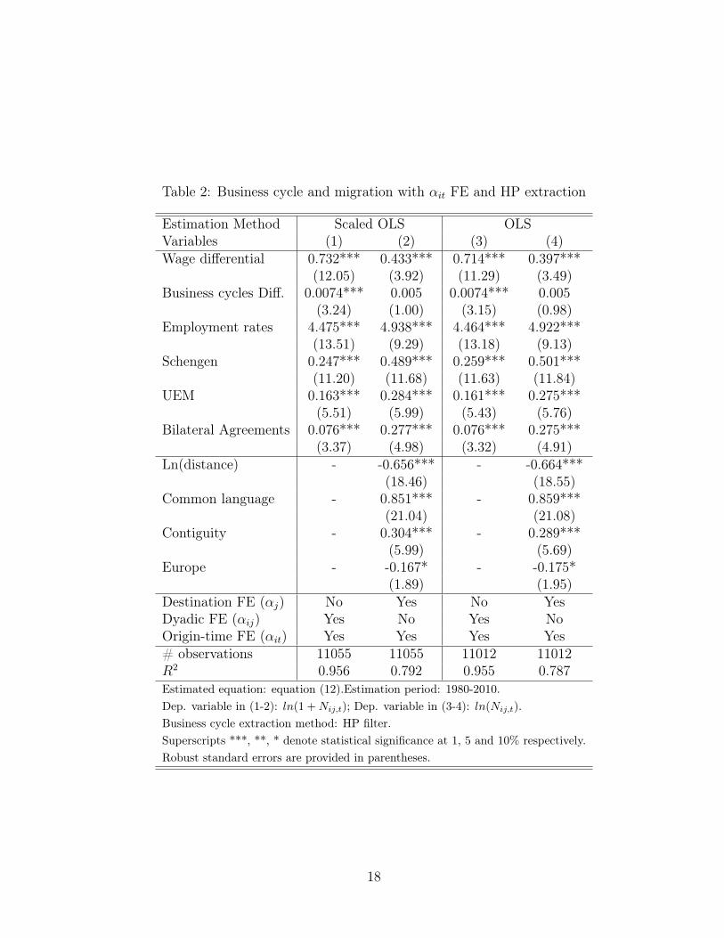
Table 2: Business cycle and migration with αit FE and HP extraction

Estimation Method Scaled OLS OLSVariables (1) (2) (3) (4)Wage differential 0.732*** 0.433*** 0.714*** 0.397***

(12.05) (3.92) (11.29) (3.49)Business cycles Diff. 0.0074*** 0.005 0.0074*** 0.005

(3.24) (1.00) (3.15) (0.98)Employment rates 4.475*** 4.938*** 4.464*** 4.922***

(13.51) (9.29) (13.18) (9.13)Schengen 0.247*** 0.489*** 0.259*** 0.501***

(11.20) (11.68) (11.63) (11.84)UEM 0.163*** 0.284*** 0.161*** 0.275***

(5.51) (5.99) (5.43) (5.76)Bilateral Agreements 0.076*** 0.277*** 0.076*** 0.275***

(3.37) (4.98) (3.32) (4.91)Ln(distance) - -0.656*** - -0.664***

(18.46) (18.55)Common language - 0.851*** - 0.859***

(21.04) (21.08)Contiguity - 0.304*** - 0.289***

(5.99) (5.69)Europe - -0.167* - -0.175*

(1.89) (1.95)Destination FE (αj) No Yes No YesDyadic FE (αij) Yes No Yes NoOrigin-time FE (αit) Yes Yes Yes Yes# observations 11055 11055 11012 11012R2 0.956 0.792 0.955 0.787Estimated equation: equation (12).Estimation period: 1980-2010.Dep. variable in (1-2): ln(1 +Nij,t); Dep. variable in (3-4): ln(Nij,t).Business cycle extraction method: HP filter.Superscripts ***, **, * denote statistical significance at 1, 5 and 10% respectively.Robust standard errors are provided in parentheses.

18

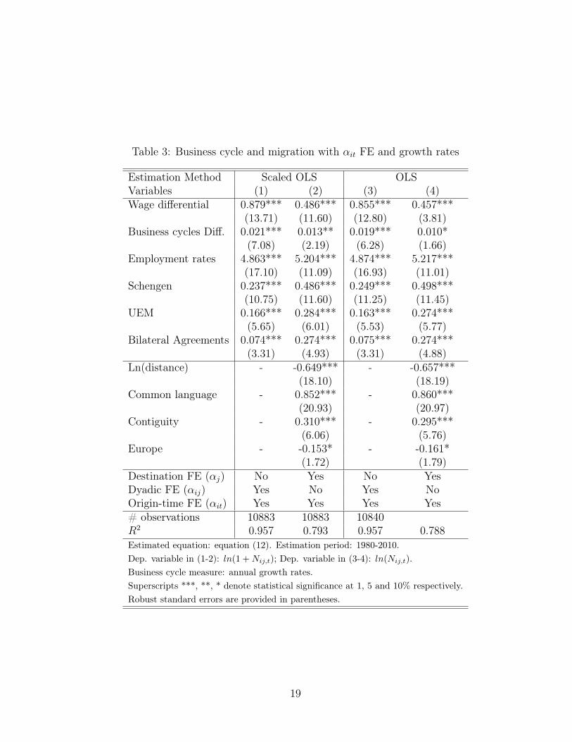
Table 3: Business cycle and migration with αit FE and growth rates

Estimation Method Scaled OLS OLSVariables (1) (2) (3) (4)Wage differential 0.879*** 0.486*** 0.855*** 0.457***

(13.71) (11.60) (12.80) (3.81)Business cycles Diff. 0.021*** 0.013** 0.019*** 0.010*

(7.08) (2.19) (6.28) (1.66)Employment rates 4.863*** 5.204*** 4.874*** 5.217***

(17.10) (11.09) (16.93) (11.01)Schengen 0.237*** 0.486*** 0.249*** 0.498***

(10.75) (11.60) (11.25) (11.45)UEM 0.166*** 0.284*** 0.163*** 0.274***

(5.65) (6.01) (5.53) (5.77)Bilateral Agreements 0.074*** 0.274*** 0.075*** 0.274***

(3.31) (4.93) (3.31) (4.88)Ln(distance) - -0.649*** - -0.657***

(18.10) (18.19)Common language - 0.852*** - 0.860***

(20.93) (20.97)Contiguity - 0.310*** - 0.295***

(6.06) (5.76)Europe - -0.153* - -0.161*

(1.72) (1.79)Destination FE (αj) No Yes No YesDyadic FE (αij) Yes No Yes NoOrigin-time FE (αit) Yes Yes Yes Yes# observations 10883 10883 10840R2 0.957 0.793 0.957 0.788Estimated equation: equation (12). Estimation period: 1980-2010.Dep. variable in (1-2): ln(1 +Nij,t); Dep. variable in (3-4): ln(Nij,t).Business cycle measure: annual growth rates.Superscripts ***, **, * denote statistical significance at 1, 5 and 10% respectively.Robust standard errors are provided in parentheses.

19

Before looking specifically at the key parameters estimates we should look at a comparisonbetween the two alternative specifications, i.e. on the one hand the specification with αij fixedeffects and on the other hand the model with αj fixed effects and observable time-invariantfactors. A straightforward comparison reveals that the share of explained variability by thefirst specification significantly outperforms the second one, with R2 close to 0.96 instead of0.80. This suggests that there are many other unobserved time-invariant dyadic factors thatare not accounted for in the second specification but which are captured in the first. Again,this suggests that interpretations based on results reported in columns (1) and (3) of tables 3and 4 are the most reliable.Overall, we find evidence in favour of long-run and short-run factors on the bilateral migra-tion flows. First, and importantly, we find a very robust and stable elasticity for the wagedifferential. An increase of around 10% in the wage ratio leads on average to an increase inthe bilateral migration flows of about 8.5% (see Table 4). Nevertheless, on top of that, we findsupport for a role of short-run factors, i.e. of business cycles and employment rates. Startingwith the specification including the αij fixed effects, the positive impact of the relative busi-ness cycles is observed regardless of the business cyclical stance measure. The same holds forthe differential employment rates. These results are consistent with the idea developed in ourtheoretical framework that the cyclical stance provides an additional signal to the candidatesto migration for choosing the optimal destination. According to this interpretation, this sig-nal is in terms of the future probability of employment for those migrants, which ultimatelyaffects the expected wage at destination and in turn the net gain derived from moving to thatdestination.The estimation results suggest that short-run factors contribute to the understanding of thevariability of bilateral migration flows. Depending on the estimation method, the decreasein the Root Mean Square Error when adding those factors is around 3.5%. While this cansound as a modest contribution, one should not forget that the model accounts for manyunobserved factors through the set of fixed effects. While the business cycle seems to enterin migrants’ expectations of future employment rates, the relative contribution seems to comemostly from the current employment rates. In terms of economic magnitudes, a rise of 1% inthe ratio of employment rates between the destination and the origin leads to a 5% increasein the bilateral migration rates. The estimated business cycle elasticities suggest that a 1%differential in growth rates between the origin and the destination countries leads to a 0.02%increase in the bilateral migration flow. Even though these orders of magnitude seem to bemodest, the cumulated effects over the whole business cycle can be substantial, especially formigration corridors that are already important.To give a more tangible assessment of the impact of employment rates, one may for instanceconsider the flows from Germany to Italy, which represented between 8,000 and 14,000 mi-grants over the considered period. Using the fact that a 1% increase in the ratio of employmentrates leads to a 5% increase in bilateral migrations rates, we find that the rise of the ratio ofemployment rates, cumulated between 2000 and 2005 (+6.5 points) contributed to a supple-mentary cumulated flow of immigrants from Germany of 3,740 persons (620 in average peryear). Conversely, when the situation reversed between 2006 and 2008, with a cumulated de-crease of the ratio of employment rates of -3 points, this contributed to a cumulated decreaseof immigration flows from Germany to Italy of 1,800 persons (600 persons in average peryear). Yet, the contribution of the differential in growth rates between the two countries wasnegligible for this couple of partners. To get more substantial contributions of the differentialin growth rates, we can take for example the flows from Romania to Spain, which rose up toaround 174,000 in 2007. Between 2001 and 2008, with growth rates that were significantlymore important in Romania than in Spain, the differential in growth rates contributed to a

20

cumulated diminution of around 500 immigrants. To take another case, the contribution ofthe differential in growth rates between Germany and Poland, which was in favor of Polandbetween 2002 and 2009, contributed to a cumulated diminution of around 800 immigrantsfrom Poland to Germany, to be compared with annual flows representing between 100,000 and160,000 immigrants a year: the comparison between the two shows a contribution which isnot negligible in absolute terms, but remains limited in proportion of the magnitude of annualflows.An important by-product of our estimation is the impact of the time-varying dyadic factorsaffecting the migration costs. We find a positive impact on mobility for the Schengen agree-ments between European countries, a positive role for currency unification as well as a positiveimpact for the other bilateral agreements. The first two results are important in terms of ourdiscussion about the optimal nature of the European Monetary Union. The traditional Opti-mum Currency Area literature (Mundell, 1961; De Grauwe, 2009) emphasized the importantrole of labour mobility in coping with asymmetric business cycle shocks. Our estimation resultsshow that with respect to labour mobility, the Schengen agreement as well as the inception ofthe Euro made Europe closer to an Optimum currency area. This of course does not mean thatEurope is or has become an OCA. Nevertheless it shows that integration measures increasedthe net gains (or decreased the net costs) derived from introduction of the Euro. For example,migration flows from the Netherlands to Belgium, which amounted to around 6,000 in thenineties rose to 12,000 in 2007. The corresponding impact of the euro area, equal to 17.4%(Cf. tables 3 and 4), would thus represent around 1,000 migrants .28 Also, the results are inline with the new OCA literature that shows that the optimal nature of a monetary unionis itself endogenous with the monetary unification process (Frankel and Rose, 1998; Beetsmaand Giuliodori, 2010). Frankel and Rose (1998) show that the optimality of a currency uniondepends on the degree of asymmetric shocks within the union, which itself depends on themonetary unification process. The same holds for the intensity of trade flows. Related to thosefindings, we show that currency unification decreases the costs of moving between Euro areacountries, and therefore increases the scope of labour mobility as an alternative adjustmentmechanism to the flexibility in exchange rates.The estimates relating to the bilateral agreement in columns (1) and (3) of Tables 2 and 3 areall found positive, which is more in line with the expected impact of bilateral agreements on themigration costs. We find that the existence of bilateral agreements favouring worker mobilitybetween two countries raises the bilateral migration flow by 7 to 8 %. The positive semi-elasticity obtained in this specification, as opposed to the negative elasticity yielded by theformer model, suggests that the current model does a better job in accounting for importantdeterminants. We will further assess the relevance of the model, particularly regarding thevalidity of the IIA assumption.Turning to the specification involving time-invariant dyadic observable variables (columns 2and 4 of Tables 2 and 3), we find evidence in favour of a role of the usual determinants suchas distance, contiguity and common language. The insignificant impact of Europe is moresurprising but might be rationalized at least in two ways. First, the role of European integra-tion is already captured by the Schengen agreements and the EMU membership. Second, theresults should be viewed with caution for the reasons mentioned above, namely, the obviousscope for a mis-specified model due to omitted time invariant dyadic factors.

28Since the coefficient of the euro area variable is related to a dummy, the corresponding elasticity cannot beused directly and is equal to (exp(0.16)-1)=0.174.To take another case, flows from Germany to Italy, between8,000 and 10,000 in the nineties, rose up to 14,000 in 2004, with a contribution of the euro area that wouldthus represent around 1,500 migrants.

21

An indirect way of testing for the validity of the IIA assumption is to look at the stability ofestimated coefficients when some destinations are dropped from the estimation sample. Thismethod was used, for example, by Head et al. (1995) for an analysis of location choices inthe US by Japanese manufacturing firms during the 1980’s. We implement this method bydropping one destination at a time and by plotting the estimated coefficients. Before examiningthe patterns of coefficients, two comments are in order. First, we rely on visual examinationonly rather than on a formal test because our sample is strongly unbalanced. It is unbalancedin several ways. For some country pairs, there may be missing years. For some origins, theremight be missing destinations for the whole time period, and for some destinations, there mightalso be missing origins. Therefore, the removal of different destinations might lead to quitedifferent subsamples. For instance, since the US is the most important destination, removingthe US reduces the sample by a maximum number of observations (30*29=870 data points).In contrast, removing Romania has little impact on the sample as the Romanian destinationis widely unavailable for most origins. Tests of equality of estimates with different subsamplesare therefore difficult to implement. Second, the fact that removing different destinations leadsto different subsamples means that our evaluation of the IIA assumption is done assumingthat there is no selection issue here. This late assumption might of course be too strong.Figures 5, 6, 7 and 8 reported in Appendix C plot the evolution of the estimated key coefficientsof equation (12) when dropping successively one destination country from the regression.29

Overall, with few exceptions in terms of destinations (Spain) and in terms of coefficients (β̂2)of equation (12), the rolling estimates display quite stable estimated coefficients.30 Comparingthe key estimated coefficients of Table 3 with the range displayed in those figures, we find thatin general the estimated impact is robust to the exclusion of alternative destinations. Theestimate of the wage differential elasticity (0.88) lies in the middle of the range in terms of thecoefficients displayed in Figure 5. The same basically holds for the other coefficients of interest,particularly those related to the employment rate differential, the business cycle differentialand the Schengen agreements.

4.3 Focusing on destination driven shocks

While specification (12) yields better estimation results, the inclusion of the αit raises a numberof statistical issues. One of them is the high degree of collinearity between the αit and thetime-varying dyadic variables such as the wage differential, the differential in business cyclesand the differential in employment opportunities. In other terms, while accounting for manyunobserved factors, the inclusion of αit eliminates much of the variability of those variablesdue to the fact that they are built using time-varying origin specific variables. This mightresult in a magnification of the standard errors of those variables and, in turn, a decrease inthe significance of the variables. A second aspect is that the business cycle considerations andemployment prospects that agents take into account could be essentially destination specific.It is possible that agents will consider migrating to destination countries with higher wagesif the employment prospects are good enough, regardless of the cyclical stance of the origineconomy. If so, what matters are destination-specific shocks. The specification implied by

29The measure of the cycle differential is given by the differential in growth rate.30More precisely, the removal of Spain from the sample tends to decrease the magnitude of the impact of the

employment differential (but not its statistical significance). This can be rationalized by the fact that Spainis precisely a country having attracted a lot of migrants due to the economic boom and an improving labourmarket, especially in the 90’s and the years prior to the financial crisis. This is well documented in Bertoliand Fernandez-Huerta Moraga (2013a).

22

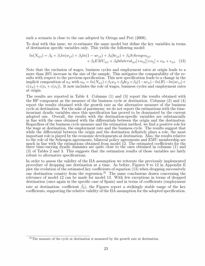
such a scenario is close to the one adopted by Ortega and Peri (2009).To deal with this issue, we re-estimate the same model but define the key variables in termsof destination specific variables only. This yields the following model:

ln(Nij,t) = β0 + β1ln(wj,t) + β2ln(1− urj,t) + β3(bcj,t) + β4Schengenij,t+ β5EMUij,t + β6bilateralij,t[+αij][+αj] + αit + εij,t (13)

Note that the exclusion of wages, business cycles and employment rates at origin leads to amore than 20% increase in the size of the sample. This mitigates the comparability of the re-sults with respect to the previous specification. This new specification leads to a change in theimplicit composition of αit with αit = ln(Nii,t)+β1wit+β2bcit+β3(1−urit)−ln(B)−ln(uri,t)+c(xit) + c(xi+ c(xt)). It now includes the role of wages, business cycles and employment ratesat origin.The results are reported in Table 4. Columns (1) and (3) report the results obtained withthe HP component as the measure of the business cycle at destination. Columns (2) and (4)report the results obtained with the growth rate as the alternative measure of the businesscycle at destination. For the sake of parsimony, we do not report the estimations with the time-invariant dyadic variables since this specification has proved to be dominated by the currentadopted one. Overall, the results with the destination-specific variables are substanciallyin line with the ones obtained with the differentials between the origin and the destination.Regardless of the business cycle measure and the estimation method, we find a positive role forthe wage at destination, the employment rate and the business cycle. The results suggest thatwhile the differential between the origin and the destination definitely plays a role, the mostimportant role is played by the economic developments at destination. Also, the results relativeto the role of the Schengen agreements, bilateral policy agreements and EMU membership aremuch in line with the estimations obtained from model 12. The estimated coefficients for thethree time-varying dyadic dummies are quite close to the ones obtained in columns (1) and(3) of Tables 2 and 3. This suggests that the estimation results of those variables are fairlyrobust to alternative specifications.In order to assess the validity of the IIA assumption we reiterate the previously implementedprocedure of dropping one destination at a time. As before, Figures 9 to 12 in Appendix Eplot the evolution of the estimated key coefficients of equation (13) when dropping successivelyone destination country from the regression.31 The same conclusions drawn concerning therelevance of model 12 can be made for model 13. With few exceptions in terms of droppeddestination (once again in the specific case of Spain) and in terms of coefficients (employmentrate at destination- coefficient β̂2), the Figures report a strikingly stable range of the keycoefficients, supporting the relative validity of the IIA assumption for the adopted specification.

31The measure of the cycle at destination is measured by the growth rate at destination.

23

Table 4: Business cycles and migration: destination specific variables

Estimation Method Scaled OLS OLSVariables (1) (2) (3) (4)Wage 0.766*** 0.903*** 0.736*** 0.872***

(13.40) (15.04) (12.45) (13.99)Business cycle 0.0067*** 0.019*** 0.0068*** 0.018***

(2.91) (6.77) (2.91) (6.11)Employment rate 5.250*** 5.614*** 5.223*** 5.611***

(14.52) (18.32) (14.37) (10.70)Schengen 0.252*** 0.243*** 0.262*** 0.252***

(11.66) (11.25) (12.03) (11.63)UEM 0.137*** 0.139*** 0.139*** 0.140***

(4.88) (4.99) (4.94) (5.03)Bilateral 0.097*** 0.095*** 0.094*** 0.094***

(4.36) (4.27) (4.22) (4.20)Destination FE (αj) No Yes No YesDyadic FE (αij) Yes No Yes NoOrigin-time FE (αit) Yes Yes Yes Yes# observations 13483 13277 13416 13211R2 0.952 0.952 0.951 0.951Estimated equation: equation (13).Estimation period: 1980-2010.Dep. variable in (1-2): ln(1 +Nij,t); Dep. variable in (3-4): ln(Nij,t).Business cycle measure: (1) and (3): HP filter.Business cycle measure: (2) and (4): Annual growth rates.Superscripts ***, **, * denote statistical significance at 1, 5 and 10% respectively.Robust t-stats are provided in parentheses.

24

4.4 Caveats: endogeneity and network effect

4.4.1 Endogeneity

One traditional concern in terms of estimation of models such as models 12 and 13 is theoccurrence of endogeneity. In particular, given the focus of the paper, the potential endogeneityof the aggregate fluctuations should be assessed with great care. For the sake of understanding,it is nevertheless important to identify the sources of endogeneity in this context. Basically,two traditional sources can be considered : (i) reverse causality from international migrationto aggregate fluctuations and employment rates and (ii) endogeneity due to omission of factorsthat could be correlated with aggregate fluctuations, namely unilateral immigration policies.

4.4.2 Reverse Causality

One particular concern is whether international migration can affect the economic conditions,i.e. whether there is a reverse causal relationship from international migration to economicfluctuations and employment rates. One important reason for which this concern is mitigatedhere is that we rely on bilateral migration flows. Migration flows at the bilateral level remainquite modest with respect to the size of the labour market and the goods market, either atorigin and at destination. To illustrate, in our sample, only 7 bilateral flows out of 870 are overthe 50000 threshold. Out of those 7 flows, 4 flows concern Germany as the destination country,with obviously one outlier in the case of Polish migrants in 1989 after the fall of the Berlinwall. Only 37 country pairs involve flows that are over 20000 migrants. Those figures suggestthan even if economic migration can affect economic outcomes in general, the bilateral natureof our analysis makes this concern much less serious than in unilateral analysis of migration.Even in the unilateral case, the literature is in general very mixed about the potential effect ofimmigration. To illustrate, the huge literature about the impact of immigration on domesticwages (Borjas, 2006; Card, 2005, Ottaviano and Peri, 2012) is divided about the exact natureof that effect. When conclusions in favour of some effects are drawn, the expected magnitudeon domestic wages remains quite modest in economic terms.

4.4.3 Omission of unilateral immigration policies

In the estimation of models 12 and 13, immigration policies are explicitly accounted by theSchengen agreements among European countries as well as by the additional bilateral agree-ments captured by the IOM database. These variables refer to bilateral policies, i.e. policiesthat are specific to a particular migration corridor. They include preferential treatments oftengranted by the host country. Due to absence of data, we do not capture explicitly the otherdimension of immigration policies, i.e. the unilateral dimension. These include immigrationpolicies that are conducted towards all the partner countries. Models 12 and 13 include αitand αij fixed effects but these do not capture the role of immigration policies conducted atdestination. One legitimate concern is that the omitted variable can lead to biased estimates.The discussion is about the expected magnitude and size of that possible bias.The bias related to the omission of immigration policies arises if these immigration policiesare contemporaneously correlated with our business cycle measures. While one can expect anegative correlation of liberal immigration policies and the business cycle over time, the tim-ing of that correlation is more debatable. A contemporaneous correlation which is needed togenerate such a bias requires that the immigration policy and its implementation reacts withina year to adverse or positive economic developments at the country level. While it might be

25

the case for some particular episodes, on average, the design and the implementation of suchimmigration policies takes time. In other terms, an underlying assumption in our estimates isthat the contemporaneous correlation between unilateral immigration policies and the cycle isquite low and requires more than a year to be of significant magnitude. Since this assumptionis important, we further assess its validity by focusing on a set of specific cases. More precisely,we focus on the cases of four important countries: United States, Canada, Spain and France.We adopt two complementary perspectives in that respect. We first consider national acts(laws, decrees, ministries’ decisions...) related to immigration that are considered in the lit-erature as potentially reactive to business cycles. We then conduct a complementary analysisof national acts concerning visas, registered in the International Organization for Migrationdatabase, and compare the dates at which these rules were passed along with peaks and toughsof economic cycles. This comparison remains qualitative since it is very difficult to numeri-cally code those acts (this depends among other things on the impact of their contents). Thisanalysis is fully detailed in the Appendix D.The analysis leads us to conclude that the contemporaneous correlation of business cyclesand unilateral immigration policies is quite low. Appendix D illustrates from case studies thevarious reasons of this low correlation. Among those reasons, even if policies account for theeconomic cycle, there is clearly a time lag needed to pass the immigration laws. Also, whilebusiness cycles might be a concern, a lot of immigration acts target non economic goals. Thisis for instance the case for family reunification policies which affect a significant proportion ofmigrants. From the whole analysis, we conclude therefore that the omission of immigrationpolicies should not invalidate the results of our empirical exercise.

4.4.4 Migrants Networks

A second source of concerns is that specifications 12 and 13 do not account for the effect ofmigrants network. Diasporas at destination are known to generate mechanisms that lower themigration costs of the natives of their countries of origin. This effect has been documented invarious papers dealing with macroeconomic data (Beine et al., 2011 among others). In thosemodels, the network is often captured by the size of the bilateral migration stock at the startof the migration period. Most of the papers consider migration periods of ten years and useeither cross sectional data (Beine et al. 2011; Bertoli and Fernandez-Huertas Moraga, 2012)or panel data (Beine and Parsons, 2012). In the context of this paper, bilateral migrationstocks are unavailable at an annual frequency, which explains the omission of the network inspecifications 12 and 13. One question is whether this is detrimental for the estimations ofour models. In that respect, some comments are in order here.First, the empirical literature emphasizes the variation of network elasticities across types ofmigration process. The network effect is obviously more important for unskilled migrants andfor South-North migration. While it is not negligible for North-North migration and skilledmigrants, the fact that we focus on migration flows among OECD countries makes the omissionof the network less important. Second, at the annual frequency, migration stocks are quitestable over time. These are for a lot of country pairs quite collinear to some fixed effects,and in particular with the dyadic ones (αij). This implies that models with αij fixed effectspartly account for some implicit network effect. Finally, our observable variable capturing thebilateral agreements is likely to be highly correlated with some of the bilateral stocks. In thatsense, part of the effect associated to the migrants networks is also reflected in the elasticityof that variable. All in all, while the inclusion of the network variables should be desirable ifdata were available, the specifications of our models and the sample of countries over whichestimations are conducted makes the omission of those effects less concerning.

26

5 Conclusion

In this paper, we empirically test the impact of macroeconomic fluctuations on migrationflows. We revisit an old issue but with a fresh approach building the recent advances inthe empirical literature on international migration. By contrast with some previous macroe-conomic approaches evaluating the degree of labour mobility through indirect evidence, weadopt a more direct approach relating gross migration flows and macroeconomic fluctuations.In particular, we rely on micro-founded gravity models that include the traditional long-rundeterminants and take into account important concepts such as the multilateral resistanceterms. Our analysis looks specifically at the sensitivity of gross migration flows to relativebusiness cycles and relative employment rates. These variables act as signals in the formationof expectations about future employment probabilities among prospective agents.In particular we find evidence that relative business cycles and employment rates affect theintensity of gross bilateral flows. We also find that the destination-specific variables such asthe business cycle or the growth rate at destination are particularly important for prospectivemigrants in choosing their optimal destination. As a by-product of this analysis, we also showthat the introduction of Schengen agreement and the inception of the common currency inEurope significantly raised the international mobility of workers between the relevant countries.These results are important as they show that compared to previous studies conducted inthe 90’s, labour mobility in Europe seems to have increased and has become more reactiveto asymmetric shocks. This dimension is key in the traditional definition of an OptimumCurrency Area. This of course does not mean that Europe has become an Optimum CurrencyArea but suggests that labour mobility as an adjustment mechanism is more a reality thanin the past. A caveat of this analysis is that we consider only homogeneous labour. Due todata constraints, we are unable to evaluate the sensitivities of agents per skills or educationlevel to business cycles. Such an investigation would indeed be a natural direction for futureresearch agenda.

27

6 References

Anderson, J. E. (2011), "The Gravity Model", Annual Review of Economics, vol. 3, pp.133-160.Anderson, J. E. and E. Van Wincoop (2003),"Gravity with Gravitas: A Solution to the BorderPuzzle", American Economic Review, vol. 69 (1), pp. 106-116.Ball, L.M., D. Leigh and P. Loungani (2013), Okun’s Law: Fit at Fifty?, NBER WorkingPaper No. 18668Baltagi, B.H. (1995), Econometric Analysis of Panel Data, Wiley, London.Beetsma, R. and M. Giuliodori (2010), The Macroeconomic Costs and Benefits of the EMU andOther Monetary Unions: An Overview of Recent Research, Journal of Economic Literature,48, 603-641.Beine, M., F. Docquier and C. Ozden (2011), "Diasporas", Journal of Development Economics,95(1), 30-41.Beine, M. and C. Parsons (2012), Climatic Factors as Determinants of International Migration,CES-IFO Working paper no. 3747.Bertoli, S. and J. Fernandez-Huerta Moraga (2013a), Multilateral Resistance to Migration,Forthcoming in Journal of Development Economics.Bertoli, S. and J. Fernandez-Huerta Moraga (2012), Visas Policies, Networks and the Cliff atthe Border, IZA Discussion Paper 2012, December.Bertoli, S., H. Brücker and J. Fernandez-Huerta Moraga (2013b), The European Crisis andMigration to Germany: Expectations and the Diversion of Migration Flows, mimeo, CERDI,University of Auvergne.Borjas, G (1987), “Self-selection and the earnings of migrants”, American Economic Review,77 (4), 531-53.Borjas, G. J, Freeman, R. B and Katz, L., 1996. "Searching for the Effect of Immigration onthe Labor Market", American Economic Review, American Economic Association, vol. 86(2),pages 246-51, May.Borjas, G.J. (2006), "Native Internal Migration and the Labor Market Impact of Immigration",Journal of Human Resources, 41(2), 221-258.Card, D., 2005. "Is the New Immigration Really so Bad?" The Economic Journal, 115, 300-323.Card, D., 2001. "Immigrant Inflows, Native Outflows, and the Local Labor Market Impactsof Higher Immigration," Journal of Labor Economics, University of Chicago Press, vol. 19(1),pages 22-64, January.Chiquiar, D. and G. Hanson (2005), "International Migration, Self-Selection, and the Distri-bution of Wages: Evidence from Mexico and the United States", Journal of Political Economy,113(2), 239-281Coulombe, S. (2006), Internal Migration, Asymmetric Shocks, and Interprovincial EconomicAdjustments in Canada, International Regional Science Review, 29(2), 199-223.De Grauwe, P. (2009), Economics of Monetary Union, 8th edition, Oxford University Press,

28

Oxford, UK.Docquier, F., A. Marfouk and B.L. Lowell (2007), a Gendered Assessment of Highly SkilledEmigration, Population and Development Review, 35, 297-322.

Docquier, F., Özden, Caglar and Peri, Giovanni, 2011. "The Labor Market Effects of Immi-gration and Emigration in OECD Countries," IZA Discussion Papers 6258, Institute for theStudy of Labor (IZA).Feenstra, R. (2004), "Advanced International Trade: Theory and Evidence", Princeton Uni-versity Press, Princeton, NJ.Frankel, J. A and Rose, A. K, 1998. "The Endogeneity of the Optimum Currency AreaCriteria", Economic Journal, Royal Economic Society, vol. 108(449), pages 1009-25, July.Green, A. G. and Green, D. (2004) "The goals of Canada’s immigration policy: a historicalperspective", Canadian Journal of Urban Research, Vol. 13(1): 102-139.Gordon, R.J. (2010), "Revisiting and Rethinking the Business Cycle, Okun’s Law and Pro-ductivity Innovations", American Economic Review, 11-15.Grogger, J., and G.H. Hanson, (2011), "Income Maximization and the selection and sortingof international Migrants, Journal of Development Economics, 95(1), 42-54.Hatton, T. J. and J. G., Williamson, (2002) "What Fundamentals Drive World Migration?".NBER Working Paper Series, Vol. w9159, 2002.Head, K., J. Ries and D. Swenson (1995), Agglomeration Benefits and Location Choice: Evi-dence from Japanese manufacturing investments in the United States, Journal of InternationalEconomics, 38, 223-247.Head, K., T., Mayer and J., Ries, (2010). "The erosion of colonial trade linkages after inde-pendence," Journal of International Economics, Elsevier, vol. 81(1), pages 1-14, May.Heston, A., R., Summers and B., Aten, (2011), "Penn World Table Version 7.0", Center forInternational Comparisons of Production, Income and Prices at the University of Pennsylvania.Lee J. (2000), The Robustness of Okun’s law: Evidence from OECD countries, Journal ofMacroeconomics, 22, 331-356Martin, S. and Lowell B. L., (2005), "Competing for skills: US immigration policy since 1990",Law and Business Review of the AmericasMayda, A. M., (2008), "International migration: A panel data analysis of the determinants ofbilateral flows", Journal of Population Economics.McFadden, D. (1984), “Econometric analysis of qualitative response models”, in: Z. Grilichesand M. Intriligator, eds., Handbook of Econometrics, Volume 2, Amsterdam. Elsevier/North-Holland.McKenzie, D., C. Theoharides and D. Yang (2010), How Important are Macro Shocks inDetermining Migration Flows? Evidence from Filipino Migration. Paper presented at the 2ndMigration and Development Conference, Paris School of Economics, June 2010.McKenzie, D. and H. Rapoport (2010), “Self-selection patterns in Mexico-US migration: therole of migration networks”, Review of Economics and Statistics, 92(4), 811-821.OECD (2009), "Migrations internationales et crise économique, comprendre les liens et éla-borer des politiques appropriées"

29

OECD (2007), International Migration Outlook 2007. Paris: Organisation for Economic Co-operation and DevelopmentO’Rourke, K. and Sinnott, R. (2006), "The determinants of individual attitudes towardsimmigration"’, European Journal of Political Economy, 22 838-861.Ortega, F., and G., Peri, (2009), "The Causes and Effects of International Migrations: Evi-dence from OECD Countries 1980-2005". NBER Working Paper Series, w14833.Ottaviano, G. and Peri, G. (2012), "Rethinking the Impact of Immigration on Wages", Journalof the European Economic Association, 10(1), 152-197.

Özden, C., C. Parsons, M. Schiff, and T. Walmsley, (2011) "Where on Earth is Everybody?",World Bank Economic Review, vol. 25(1), 13-58.Pedersen, P.J., Pytlikova M. and Smith N. (2008),. "Selection and network effects-Migrationflows into OECD countries 1990-2000", European Economic Review, 52 (7), 1160-1186.Roy, A.D. (1951), “Some thoughts on the distribution of earnings”, Oxford Economic Papers,3 (2), 135-46.Rosenzweig, M. R. (2006), The Circulation Migration of the Skilled and Economic Develop-ment, Proceedings Federal Reserve Bank of Dallas, 147-170.Santos Silva, J.M.C. and S. Tenreyro (2006), "The Log of Gravity", Review of Economics andStatistics, 88 (4): 641-658.Simpson, N. and C. Sparber (2012), The Short- and Long-Run Determinants of Less-EducatedImmigrant Flows into U.S. States, Colgate University, Mimeo.

30

Appendix A: Data sources and details

Two sources are used: the international migration flows dataset from the UN 32 and the OECDInternational Migration database.33 These two databases give us, for all destination countries,migrant inflows by origin country. They both aggregate information registered at countrylevel. The fact that national authorities use different processes of data collection and that wehave associated two different sources of data naturally raises a number of data comparabilityproblems.The first is geographic and time coverage. Few countries provide data for all origincountries over the whole period (1980-2010); however in our final selection we retained onlycountries that provided data on a substantial number of destinations and over a significantperiod. Another issue relates to the definition of migrant flows because national authoritiesuse three distinct criteria to register immigrants. We tried to keep the same criterion for allcountries in order to obtain as harmonized a sample as possible.Most countries in our sample use the residence criterion, others use the citizenship criterionand only one country uses the birth-place criterion.34 The last issue refers to particular migrantgroups. Some countries register only foreign migrants and do not count citizens who migrateback.35 The residence criterion gives us a better appreciation of short-term mobility since itcaptures migrants’ last country of residence, while citizenship and birth-place criteria capturerespectively long-term immigrants and their country of origin. The residence criterion involvesthe delivery of a residence permit, and the duration of that permit varies between countries.36

However, it is important to remember that the date of a residence permit may or may notcoincide with a migrant’s date of arrival in a country.Total population Ni,t in a given country i at year t is obtained from the World PopulationProspects: the 2010 Revision database. This database is produced by the Population Division(Department of Economic and Social Affairs) of the United Nations. Data cover total popula-tions (both sexes combined) of major countries, on an annual basis, from 1950 to 2010. The cor-responding data can be viewed at http://esa.un.org/unpd/wpp/Excel-Data/population.htmAnnual data relating to GDP, unemployment and wages (more precisely hourly wages in themanufacturing sector) are taken from the World Economic Outlook data of the InternationalMonetary Fund. Wages series most often start from the beginning of the period under review(1980) but are sometimes available later (for the Czech Republic, Slovenia or even UnitedKingdom) or may be missing completely (Russia). Unemployment data are more complete,but may also begin after 1980 in the case of Eastern European countries.Before merging migration series and other data, we applied statistical controls on migrationsto search for potential problems. In particular, we checked the years in which there was astrong increase or decrease compared to data in the rest of the period, for most significantflows (above 1,000 migrants on average). Indeed, flows may possibly increase from 1 migrantto 10 migrants in the following year; but an increase from 10,000 to 100,000 migrants for acouple of countries and over two consecutive years is far more unlikely. Having identified a few

32This dataset is provided by United Nations Population division. More information may be found onhttp://www.un.org/esa/population/migration/ .

33Downloadable on http://stats.oecd.org/34For countries for which it was possible, we checked the variation between alternative criteria. This was

acceptable for the countries of the sample.35We also checked that this, in terms of migrant definition, would not be an issue for our analysis.36More information is available on http://www.un.org/esa/population/migration/CD-

ROM%20DOCUMENTATION_UN_Mig_Flow_2010.pdf

31

cases, we have checked for possible political or economic reason to retain the data. In cases ofdoubt, we have replaced the series by missing data. Conversely, when a series was very stablewith a missing point during the period, we have interpolated the values of the preceding andthe following year. We have also checked for the comparability of migrations flows betweenthe different concepts (residence, birth-place and citizenship).

Data sources and detailsDestinationCountry Sources Period Origin Countries

Migration criterion & cat-egory

Australia UN 1980-2008 All origin countriesResidence, foreigners andcitizens

Austria UN 1996-2009 All origin countries Residence, foreignersBelgium UN 1980-2007 All origin countries Citizenship, foreignersCanada UN 1980-2009 Other origin countries Residence, foreigners

1992-2009 Croatia, Russian Federation, Slovenia1993-2009 Slovakia

Croatia UN 1992-2009 Other origin countries Residence, foreigners and citizens1999-2009 New Zealand2002-2009 France, Hungary, Netherlands

2008-2009Belgium, Czech Republic, Russian Federation, Slo-vakia, United Kingdom

Not available

Denmark, Finland, Greece, Iceland, Ireland, Israel,Luxembourg, Norway, Portugal, United Kingdom,United States

Czech Republic UN 1993-2007 Other origin countries Residence, foreigners and citizens1994-2007 Croatia, Slovenia, Israel2001-2007 Ireland2004-2007 Iceland, Luxembourg, New Zealand, Portugal

Denmark UN 1980-2009 Other origin countries Residence, foreigners and citizens1992-2009 Croatia, Russian Federation, Slovenia1993-2009 Czech Republic, Slovakia

Finland UN 1987-2009 Other origin countries Residence, foreigners and citizens1992-2009 Croatia, Russian Federation, Slovenia, Slovakia1993-2009 Czech Republic

France UN 1994-2003 Other origin countries Citizenship, foreigners

1994-2006

Australia, Canada, Czech Republic, Croatia, Hun-gary, Israel, New Zealand, Romania, Russian Federa-tion, Slovakia, Slovenia, United States

1994-2008 SwitzerlandGermany UN 1980-2009 Other origin countries Residence, foreigners and citizens

1992-2009 Croatia, Russian Federation, Slovenia1993-2009 Czech Republic, Slovakia

Greece OECD 1985-2001; 2006 United Kingdom Residence, foreigners1988-2009 Belgium, Germany, Sweden1995-2009 Hungary, Norway1996-2009 Canada, Luxembourg

1997-2009Australia, Denmark, Finland, Spain, Switzerland,United States

1998-2000 Italy1998-2009 Austria, Israel2000-2009 Netherlands2003-2009 Slovakia2006-2009 New Zealand

Not availableCroatia, Czech Republic, France, Iceland, Ireland,Portugal, Romania, Slovenia

Hungary UN 1995-2008 Other origin countries Citizenship, foreigners

2008Australia, Czech Republic, Iceland, New Zealand,Slovenia

Iceland UN 1986-2010 Other origin countries Residence, foreigners and citizens1993-2010 Russian Federation, Slovenia1995-2010 Slovakia

Ireland OECD 1982-2009 United States Residence, foreigners1985-2001; 2009 United Kingdom1990-2009 Belgium1991-2009 Australia1995-2009 Germany, Hungary, Norway1996-2009 Canada, Luxembourg1997-2009 Denmark, Finland, Spain, Switzerland1998-2009 Austria2000-2009 Netherlands, Sweden2003-2009 Slovakia2006-2009 New Zealand

Not available

Croatia, Czech Republic, France, Greece, Iceland,Israel, Italy, Portugal, Russian Federation,Romania,Slovenia

Israel UN 1995-2009 Other origin countries Residence, foreigners1995-2001; 2009 Russian Federation2000 Ireland, Norway2000-2001 Australia, Denmark, Finaland, New Zealand, Sweden

Not availableCroatia,Czech Republic, Iceland, Luxembourg, Por-tugal, Slovakia, Slovenia

Italy UN 1995-2008 All origin countriesResidence, foreigners andcitizens

Luxembourg OECD 1995-2009 Germany, Hungary Residence, foreigners1996-2009 Canada1997-2008 Denmark

1997-2009Australia, Finland, Norway, Spain, Switzerland,United States

1998-2009 Austria2000-2009 Netherlands, Sweden2005-2009 Slovakia2006-2009 New Zealand2008-2009 Belgium

Not available

Croatia, Czech Republic, France, Greece, Ireland,Italy, Portugal, Romania, Russian Federation, Slove-nia, United Kingdom

Netherlands UN 1980-2009 Other origin countries Citizenship, foreigners1992-2009 Croatia, Russian Federation, Slovenia

32

1993-2009 Czech Republic, SlovakiaNew Zealand UN 1980-2010 Other origin countries Residence, foreigners and citizens

1993-2010Croatia, Czech Republic, Russian Federation, Slove-nia

1993-2010 SlovakiaNorway UN 1986-2009 Other origin countries Residence, foreigners and citizens

1992-2009 Croatia, Russian Federation, Slovenia1993-2009 Czech Republic, Slovakia

Portugal OECD 1985-1989; 1995-2001 United Kingdom37 Residence, foreigners1986-2009 United States1988-2009 Belgium, Germany, Luxembourg, Switzerland1991-2009 Australia1995-2009 Hungary, Norway1996-2009 Canada, Finland1997-2008 Denmark1997-2009 Spain2000-2009 Netherlands2003-2009 Slovakia2006-2009 New Zealand

Not available

Croatia, Czech Republic, France, Greece, Ireland,Iceland, Israel, Italy, Romania, Russian Federation,Slovenia

Romania UN 1994-2009Canada, France, Germany, Hungary, Israel, Italy, Ro-mania Residence, foreigners and citizens

2001-2008 Other origin countries

Russian Federation UN 1991-2009Australia, Canada, Germany, Greece, Finland, Swe-den Residence, foreigners and citizens

1991-2010 Israel, United StatesNot available Other origin countries

Slovakia UN 1993-2009 All origin countriesResidence, foreigners andcitizens

Slovenia UN 1996-2009 Austria Citizenship, foreigners

1998-2008Ireland, Iceland, Israel, Luxembourg, Norway, NewZealand, Portugal, Spain, Slovakia

1998-2009 Other origin countriesSpain UN 1983-2010 Other origin countries Residence, foreigners and citizens

1985-2010 Italy1983-84; 2005-10 Norway1985-1987; 1995-2010 Finland1988-2010 Greece1992-2010 Romania1994-2000; 2005-2010 Croatia1994-2010 Czech Republic, Slovakia, Slovenia1996-2010 Russian Federation2001-2010 Hungary2006-2010 Iceland, Israel, New Zealand

Sweden UN 1980-201038 Other origin countries Residence, foreigners and citizens1991-2010 Russian Federation1992-2010 Croatia, Czech republic, Slovenia1994-2010 Slovakia

Switzerland UN 1991-2009 Other origin countries Citizenship, foreigners1992-2009 Croatia, Russian Federation, Slovenia1993-2009 Slovakia

United Kingdom OECD 1980-2009 Canada, United States Residence, Foreigners1986-2003 Netherlands, Norway1988-2009 Sweden, Switzerland1991-2009 Australia, Belgium1992-2009 Finland, Portugal1994-2008 Denmark1994-2009 Ireland, New Zealand1995-2009 Germany, Hungary1996-2009 Luxembourg1997-2009 Spain1998-2004 Italy1998-2009 Austria, Israel, Slovenia2003-2009 Czech Republic, Slovakia

Not availableFrance, Greece, Ireland, Romania, Russian Federa-tion

United States UN 1980-2010 Other origin countries Birth, foreigners1992-2010 Croatia, Russian Federation, Slovenia1993-2010 Slovakia1994-2010 Czech Republic

Sources: United Nations Population division, OECD international migration database.

37We also have available data for years 1993 and 2004.38Year 1982 is not available for Greece and United Kingdom.

33

Figure2:

Total

emigrant

flowsby

coun

try

203040506070Total emigrant flow (in thousands)

1980

1990

2000

2010

Yea

rs

Aus

tral

ia


1980

1990

2000

2010

Yea

rs

Aus

tria


1980

1990

2000

2010

Yea

rs

Bel

gium


1980

1990

2000

2010

Yea

rs

Can

ada010203040

Total emigrant flow (in thousands)

1980

1990

2000

2010

Yea

rs

Cro

atia


1980

1990

2000

2010

Yea

rs

Cze

ch R

epub

lic


1980

1990

2000

2010

Yea

rs

Den

mar

k


1980

1990

2000

2010

Yea

rs

Fin

land


1980

1990

2000

2010

Yea

rs

Fra

nce


1980

1990

2000

2010

Yea

rs

Ger

man

y


1980

1990

2000

2010

Yea

rs

Gre

ece


1980

1990

2000

2010

Yea

rs

Hun

gary


1980

1990

2000

2010

Yea

rs

Icel

and


1980

1990

2000

2010

Yea

rs

Irel

and


1980

1990

2000

2010

Yea

rs

Isra

el


1980

1990

2000

2010

Yea

rs

Italy


1980

1990

2000

2010

Yea

rs

Luxe

mbo

urg


1980

1990

2000

2010

Yea

rs

Net

herla

nds


1980

1990

2000

2010

Yea

rs

New

Zea

land


1980

1990

2000

2010

Yea

rs

Nor

way


1980

1990

2000

2010

Yea

rs

Por

tuga

l


1980

1990

2000

2010

Yea

rs

Rom

ania


1980

1990

2000

2010

Yea

rs

Rus

sian

Fed

erat

ion


1980

1990

2000

2010

Yea

rs

Slo

vaki

a


1980

1990

2000

2010

Yea

rs

Slo

veni

a


1980

1990

2000

2010

Yea

rs

Spa

in


1980

1990

2000

2010

Yea

rs

Sw

eden


1980

1990

2000

2010

Yea

rs

Sw

itzer

land


1980

1990

2000

2010

Yea

rs

Uni

ted

Kin

gdom


1980

1990

2000

2010

Yea

rs

Uni

ted

Sta

tes

34

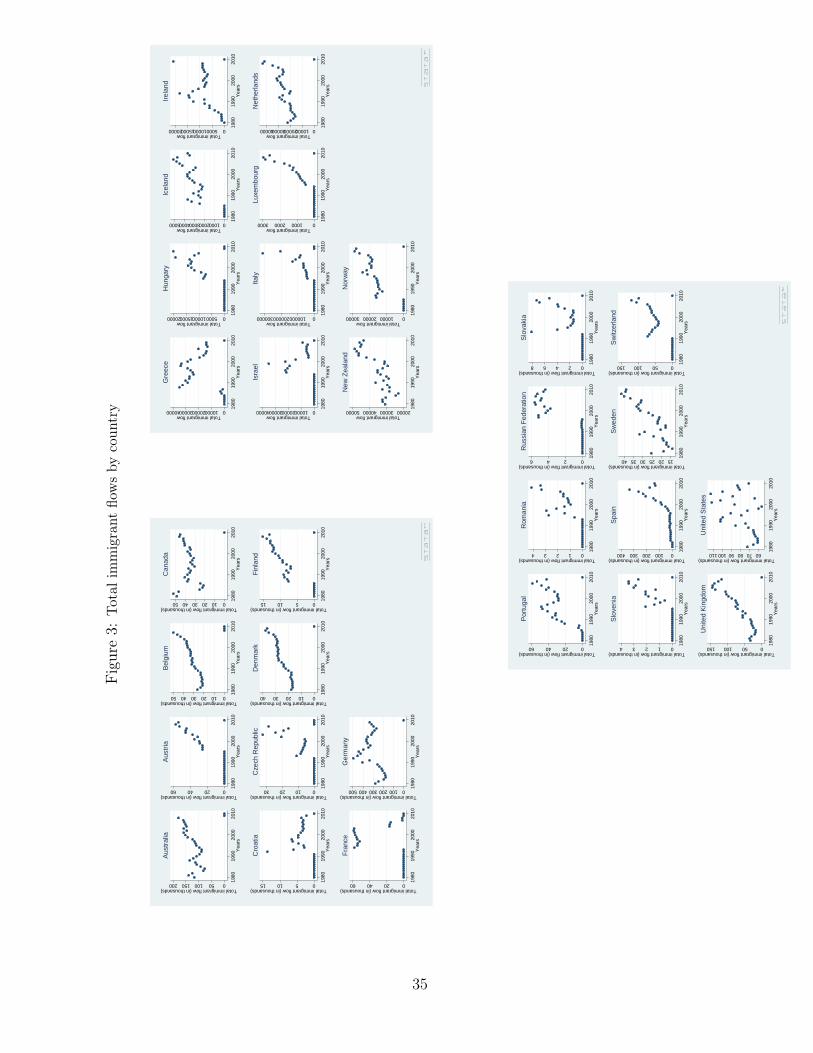
Figure3:

Total

immigrant

flowsby

coun

try

050100150200Total immigrant flow (in thousands)

1980

1990

2000

2010

Yea

rs

Aus

tral

ia


1980

1990

2000

2010

Yea

rs

Aus

tria


1980

1990

2000

2010

Yea

rs

Bel

gium


1980

1990

2000

2010

Yea

rs

Can

ada051015

Total immigrant flow (in thousands)

1980

1990

2000

2010

Yea

rs

Cro

atia


1980

1990

2000

2010

Yea

rs

Cze

ch R

epub

lic


1980

1990

2000

2010

Yea

rs

Den

mar

k


1980

1990

2000

2010

Yea

rs

Fin

land


1980

1990

2000

2010

Yea

rs

Fra

nce


1980

1990

2000

2010

Yea

rs

Ger

man

y

010000200003000040000Total immigrant flow

1980

1990

2000

2010

Yea

rs

Gre

ece


1980

1990

2000

2010

Yea

rs

Hun

gary


1980

1990

2000

2010

Yea

rs

Icel

and


1980

1990

2000

2010

Yea

rs

Irel

and


1980

1990

2000

2010

Yea

rs

Isra

el


1980

1990

2000

2010

Yea

rs

Italy


1980

1990

2000

2010

Yea

rs

Luxe

mbo

urg


1980

1990

2000

2010

Yea

rs

Net

herla

nds


1980

1990

2000

2010

Yea

rs

New

Zea

land


1980

1990

2000

2010

Yea

rs

Nor

way


1980

1990

2000

2010

Yea

rs

Por

tuga

l


1980

1990

2000

2010

Yea

rs

Rom

ania


1980

1990

2000

2010

Yea

rs

Rus

sian

Fed

erat

ion


1980

1990

2000

2010

Yea

rs

Slo

vaki

a


1980

1990

2000

2010

Yea

rs

Slo

veni

a


1980

1990

2000

2010

Yea

rs

Spa

in


1980

1990

2000

2010

Yea

rs

Sw

eden


1980

1990

2000

2010

Yea

rs

Sw

itzer

land


1980

1990

2000

2010

Yea

rs

Uni

ted

Kin

gdom


1980

1990

2000

2010

Yea

rs

Uni

ted

Sta

tes

35

Appendix B: Sources of data capturing the bilateral agree-mentsSignatory country A Signatory country B Date of

effectivenessTitle of the agreement

Switzerland Spain 1961 Accord entre la Suisse et l’Espagne sur l’engagement des travailleursespagnols en vue de leur emploi en Suisse

Switzerland Spain 1990 Echange de lettres des 9 août/31 octobre 1989 entre la Suisse etl’Espagne concernant le traitement administratif des ressortissants d’unpays dans l’autre après une résidence régulière et ininterrompue de cinqans

Switzerland France 1947 Traité de travail entre la Suisse et la FranceSwitzerland France 1958 Accord entre la Suisse et la France relatif aux travailleurs frontaliersSwitzerland Italy 1965 Accord entre la Suisse et l’Italie relatif à l’émigration de travailleurs

italiens en SuisseSwitzerland Portugal 1990 Echange de lettres du 12 avril 1990 entre la Suisse et le Portugal con-

cernant le traitement administratif des ressortissants d’un pays dansl’autre après une résidence régulière et ininterrompue de cinq ans

Switzerland 27 European members 2002 Accord entre la Confédération suisse, d’une part, et la Communautéeuropéenne et ses Etats membres, d’autre part, sur la libre circulationdes personnes

Switzerland Law concerning all foreigncountries

2006 Loi fédérale sur les étrangers

Austria Law concerning all foreigncountries

2006 Federal Act concerning settlement and residence in Austria (the Settle-ment and Residence Act-SRA)

Italy Legislative Decree con-cerning all foreigncountries

1998 Combined text of measures governing immigration and norms on thecondition of foreign citizens

United States Canada 1994 North America Free Trade Agreement

To complement international texts such as the Schengen agreements, which legally facilitatemigrations, we build a variable taking a value of 1 for a couple of countries when a bilaterallabour agreement exists between these two countries, or when a general law easing foreigners’entrance is passed. When no agreement or law exists, the variable is equal to zero.The main source is the International Organization for Migrations. The corresponding list ofagreements can be consulted at the following link: http://www.imldb.iom.int/changeLocale.doThis main source has been complemented with the information from the North America FreeTrade Agreement, which to a certain extent, facilitated labour migrations between the UnitedStates and Canada after 1994.On the other hand, important migrations exist between the members of the Commonwealth,but without any formal agreement, as confirmed in an OECD source:http://www.oecd-ilibrary.org/fr/social-issues-migration-health/migration-et-emploi_9789264108707-frIn this latter case, the variable taking into account bilateral agreements does not take thevalue of one because these agreements are only implicit and, as this situation existed alreadybefore the beginning of the period under review in our article, there is no time variance. Thus,these implicit agreements are absorbed by dyadic fixed effects.

36

Appendix C: Results from the suboptimal benchmark spec-ification.

Table 6 reports the estimates of model (11). The business cycle is measured using the de-viation of GDP from the trend extracted using the HP filter. Table 7 reports exactly thesame information, but using the annual growth rate of GDP as an alternative measure ofthe economic cycle. In each table, we use two different measures for the numerator of thedependent variable ln(Nij,t

Nii,t). The first one takes the log of 1 +Nij,t in the numerator in order

to keep the country pairs with zero observations for Nij,t in the estimation sample. This issometimes called Scaled OLS estimation (Simpson and Sparber, 2012). The second one usessimply ln(Nij,t) in the numerator as in the equilibrium condition, which leads to a modestdecrease in the sample size.39 Columns (1-4) give the estimates using ln(1+Nij,t

Nii,t) as our de-

pendent variable while Columns (5-8) give the estimates based on ln(Nij,t

Nii,t) . Columns (1) and

(5) report estimates based on the full model as given in equation (11). In columns (3) and (7)the cycle is measured only at destination while in columns (4) and (8), the business cycle andthe employment rate are both measured at the destination only.

39Actually, we have only a reduction of 43 data points, which reflects that the proportion of (true) zeroesfor the bilateral flows in our dataset is negligible. This further justifies the use of OLS estimators instead ofthe Poisson Pseudo Maximum Likelihood estimators advocated by Santos Silva and Tenreyro (2006).

37

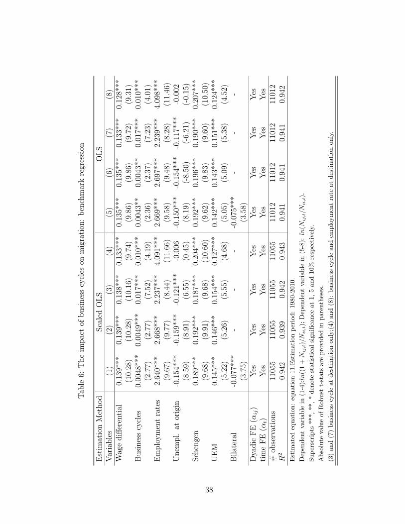
Table6:

The

impa

ctof

business

cycles

onmigration

:be

nchm

arkregression

Estim

ationMetho

dScaled

OLS

OLS

Variables

(1)

(2)

(3)

(4)

(5)

(6)

(7)

(8)

Wag

ediffe

rential

0.13

9***

0.13

9***

0.13

8***

0.13

3***

0.13

5***

0.13

5***

0.13

3***

0.12

8***

(10.28

)(10.28

)(10.16

)(9.74)

(9.86)

(9.86)

(9.72)

(9.31)

Businesscycles

0.00

48**

*0.00

49***

0.01

7***

0.010*

**0.00

43**

0.00

43**

0.01

7***

0.01

0***

(2.77)

(2.77)

(7.52)

(4.19)

(2.36)

(2.37)

(7.23)

(4.01)

Employ

mentrates

2.64

0***

2.66

8***

2.23

7***

4.09

1***

2.66

9***

2.69

7***

2.23

9***

4.09

8***

(9.67)

(9.77)

(8.44)

(11.66

)(9.58)

(9.48)

(8.28)

(11.46

)Unempl.at

origin

-0.154

***

-0.159

***

-0.121

***

-0.006

-0.150

***

-0.154

***

-0.117

***

-0.002

(8.59)

(8.91)

(6.55)

(0.45)

(8.19)

(-8.50)

(-6.21

)(-0.15

)Scheng

en0.18

9***

0.19

2***

0.18

7***

0.20

4***

0.19

2***

0.19

6***

0.19

0***

0.20

7***

(9.68)

(9.91)

(9.68)

(10.60

)(9.62)

(9.83)

(9.60)

(10.50

)UEM

0.14

5***

0.14

6***

0.15

4***

0.12

7***

0.14

2***

0.14

3***

0.15

1***

0.12

4***

(5.22)

(5.26)

(5.55)

(4.68)

(5.05)

(5.09)

(5.38)

(4.52)

Bila

teral

-0.077

***

--

--0.075

***

--

-(3.75)

(3.58)

Dya

dicFE

(αij)

Yes

Yes

Yes

Yes

Yes

Yes

Yes

Yes

timeFE

(αt)

Yes

Yes

Yes

Yes

Yes

Yes

Yes

Yes

#ob

servations

1105

511

055

1105

511

055

1101

211

012

1101

211

012

R2

0.94

20.93

90.94

20.94

30.94

10.941

0.94

10.94

2Estim

ated

equa

tion

:equa

tion

11.Estim

ationpe

riod

:1980-2010.

Dep

endent

variab

lein

(1-4):ln((1+N

ij,t)/N

ii,t);Dep

endent

variab

lein

(5-8):ln(N

ij,t/N

ii,t).

Supe

rscripts

***,

**,*

deno

testatisticals

ignifican

ceat

1,5an

d10%

respectively.

Absolutevalueof

Rob

ustt-statsareprovided

inpa

rentheses.

(3)an

d(7)bu

siness

cycleat

destinationon

ly;(4)

and(8):

business

cyclean

dem

ploymentrate

atdestinationon

ly.

38

Table7:

The

impa

ctof

business

cycles

onmigration

:grow

thrate

asameasure

ofcyclical

stan

ce

Estim

ationMetho

dScaled

OLS

OLS

Variables

(1)

(2)

(3)

(4)

(5)

(6)

(7)

(8)

Wag

ediffe

rential

0.16

6***

0.16

6***

0.16

8***

0.15

7***

0.15

0***

0.16

0***

0.16

1***

0.15

0***

(9.37)

(9.37)

(9.44)

(8.85)

(8.43)

(8.93)

(9.01)

(8.41)

Businesscycles

0.01

3***

0.01

3***

0.01

8***

0.01

5***

0.01

4***

0.01

2***

0.01

6***

0.01

3***

(6.18)

(6.08)

(7.52)

(5.07)

(4.52)

(5.38)

(5.13)

(4.35)

Employ

mentrates

2.90

0***

2.93

72.93

7***

4.634*

**4.61

7***

2.94

4***

2.94

7***

4.65

7***

(11.83

)(11.99

)(11.93

)(15.30

)(15.01

)(11.82

)(11.77

)(15.15

)Unempl.at

origin

-0.162

***

-0.167

***

-0.159

***

-0.003

0.00

5-0.162

***

-0.155

***

0.00

17(8.64)

(9.01)

(6.55)

(0.19)

(0.33)

(8.59)

(8.17)

(0.11)

Scheng

en0.18

5***

0.18

9***

0.19

0***

0.20

5***

0.20

4***

0.19

2***

0.19

3***

0.20

9***

(9.49)

(9.73)

(9.78)

(10.68

)(10.33

)(9.66)

(9.69)

(10.57

)UEM

0.14

7***

0.14

8***

0.15

0***

0.12

3***

0.11

9***

0.14

5***

0.14

6***

0.12

0***

(5.30)

(5.34)

(5.38)

(4.52)

(4.31)

(5.17)

(5.20)

(4.35)

Bila

teral

-0.086

***

--

--0.082

***

--

-(4.16)

(3.96)

Dya

dicFE

(αij)

Yes

Yes

Yes

Yes

Yes

Yes

Yes

Yes

timeFE

(αt)

Yes

Yes

Yes

Yes

Yes

Yes

Yes

Yes

#ob

servations

1088

310

883

1088

310

883

1084

010

840

1084

010

840

R2

0.94

30.943

0.94

30.944

0.94

20.941

0.94

10.942

Estim

ated

equa

tion

:equa

tion

(11).Estim

ationpe

riod

:1980-2010.

Dep

endent

variab

lein

(1-4):ln((1+N

ij,t)/N

ii,t);Dep

endent

variab

lein

(5-8):ln(N

ij,t/N

ii,t).

Supe

rscripts

***,

**,*

deno

testatisticals

ignifican

ceat

1,5an

d10%

respectively.

Absolutevalueof

Rob

ustt-statsareprovided

inpa

rentheses.

(3)an

d(7)bu

siness

cycleat

destinationon

ly;(4)

and(8):

business

cyclean

dem

ploymentrate

atdestinationon

ly.

39

Appendix D: Analysis of legal acts related to immigrationand visas

In order to analyze the impact of business cycles on migrations acts among the countries inour sample, we focus on the cases of four important countries, namely the United States,Canada, Spain and France. With this sample, two non-European and two European countriesare covered and they all have a sufficient size and/or large enough immigrations flows to besomewhat representative, though having their own characteristics.

To that purpose, we use two complementary perspectives. We first consider national acts(laws, decrees and ministerial decisions) related to immigration that are considered in theliterature as reactions to business cycles.

We also make a complementary analysis of national acts concerning visas, registered in theInternational Organization for Migration database, and compare the dates at which theserules were passed with the economic cycles. This comparison remains qualitative: we havechosen not to give a value to these rules to include them in regressions because numerical val-ues are difficult to be coded (this depends among other things on the impact of their contents).

A. Analysis of legal acts in the literatureWe first consider legal acts passed by the four countries under review, in reaction to the eco-nomic cycle, as recorded in the literature.

According to Martin and Lowell (2005), the "Canadian policy [...], relative to the U.S., favorsselection of skilled migrants and varies levels to immigration according to economic cycle."Moreover, "Unlike the U.S., where changes in admissions occur every few decades, Canadianadmission levels change following ministerial consultations. The goal historically has been toset numerical targets that vary with the economic cycle. The numbers grew toward 200,000in the 1970s only to be reduced to just over 100,000 in the mid-1980s, followed by a robustgrowth to just shy of 250,000 in the mid-1990s. Family immigrants made up an increasingshare over that time period being about half of all admissions by 1994 and the independentstream about four tenths (balance refugee). It can be argued that a 50/50 balance of skilledand family admission will yield a net benefit, or at least minimize any potential adverse impactby balancing economically versus non-economically selected immigrants [...]".40

It thus appears that Canada and United States have very different approaches: more immi-grants selection and more quantitative limits that are likely to change merely by ministerialdecisions in Canada. It does not mean that United States do not change their rules over time(Cf. graph in the following part showing national acts linked to visas recorded by the Inter-national Organization for Migration), but it is not as systematically linked to the economiccycle and not so easy to pass.

Indeed, although the United States have also set numerical limitations for employment-basedlegal permanent residents, this objective has been set by the Congress in 1990 at 140,000 immi-grants a year, and this number has not fluctuated since then. Yet, there are more fluctuationsin the United States for specific cases like temporary admissions. As stated in Martin andLowell (2005), in the Immigration Act of 1990, Congress imposed restrictions on the growing

40See also Green and Green, 2004 for a thorough analysis of the Canadian immigration policy over a longperiod of time.

40

use of the H visa, a visa originally set for temporary workers, and that concerned later onworkers with a dual intent to stay either temporarily or permanently (H- 1B visa). Theserestrictions intended to protect domestic workers. Originally, the visa had no numerical lim-itations and few labor protections. In 1990, a numerical cap of 65,000 new H- 1Bs per yearwas imposed. Yet, this limit was increased several times, especially as the result of lobbyingby the information technology industry: from 65,000 per year to 115,000 per year in 1999 and2000, and 107,500 in 2001, and then decreased later on, but not only for economic reasons(Cf. the events of 11th September 2001).

Concerning Spain, it was only in July 1985 that the government passed a law aimed at reg-ulating immigration, as it was needed before the incorporation of Spain into the EuropeanCommunity in 1986. Up to the early 1990s, Spain maintained a relatively flexible stand onthe implementation of effective policies of border closure while, simultaneously developing arestrictive legal framework in accordance with the requirements of its partners in the EuropeanUnion. This attitude changed in 1991, coinciding with the expiration of the 1964 agreementwith Morocco, and the 1966 agreement with Tunisia for the mutual suppression of visas, whenthe Spanish government reintroduced the requirement of visas for nationals of countries fromNorth Africa, as a precondition for the incorporation of Spain into the Schengen agreement.Over latest years, a sizeable part of immigration has been non qualified, especially directedtowards sectors such as construction. If Spain has decided to reduce its contingent of non-seasonal workers in 2009 (Cf. OECD (2009)), it concerned workers recruited anonymouslyabroad, thus rather non qualified workers. Thus, globally, we may say that Spanish legal acts,coming late, were rather directed towards countries mostly out of our sample, as confirmed inthe analysis of acts related to visas recorded by the International Organization for Migration(see hereafter).

France is among the countries (it is also the case in the United Kingdom for instance) thatuse lists of workforce shortage, to regulate economic immigration. These lists are based ondata related to job vacancies: if the ratio between jobs offers and available workers exceedsa certain level for more than one year (initially equal to 1, and then decreased to 0.9), theprofession is included in a regional yearly list of jobs under tension. Yet, because of this timelag of one year, this list cannot fit the economic situation in real time (Cf. OECD (2009)).France has also established lists of jobs under tension in bilateral agreements, but rather withcountries out of our sample (for example the agreement with Gabon in 2007). This policyis quite different from the one in "settlement countries" where long term needs contribute todetermine the content of these lists (like New-Zealand or to a lesser extent Canada). Fromthis point of view, France appears as adapting partly (because many immigrants still come fornon economic reasons, including from countries in our sample), though with delay, its legalframework to the economic conditions.

B. Analysis of legal acts related to visas for four countries in the database of theInternational Organization for MigrationConsidering the legal acts related to visas for four countries in the database of the InternationalOrganization for Migration, we find that national laws about visas are not changed at regularintervals and that these changes do not always take place at the same stage of the cycle. Thisis due to a large extent to time lags between an economic downturn and the moment whenpolicies are decided and voted, which may last for some time.

41

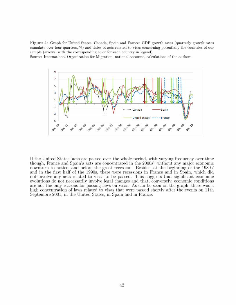
Figure 4: Graph for United States, Canada, Spain and France: GDP growth rates (quarterly growth ratescumulate over four quarters, %) and dates of acts related to visas concerning potentially the countries of oursample (arrows, with the corresponding color for each country in legend)Source: International Organization for Migration, national accounts, calculations of the authors

If the United States’ acts are passed over the whole period, with varying frequency over timethough, France and Spain’s acts are concentrated in the 2000s’, without any major economicdownturn to notice, and before the great recession. Besides, at the beginning of the 1980s’and in the first half of the 1990s, there were recessions in France and in Spain, which didnot involve any acts related to visas to be passed. This suggests that significant economicevolutions do not necessarily involve legal changes and that, conversely, economic conditionsare not the only reasons for passing laws on visas. As can be seen on the graph, there was ahigh concentration of laws related to visas that were passed shortly after the events on 11thSeptembre 2001, in the United States, in Spain and in France.

42

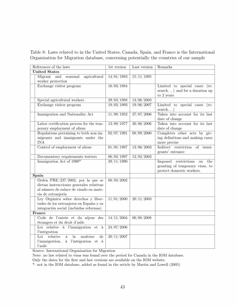
Table 8: Laws related to in the United States, Canada, Spain, and France is the InternationalOrganization for Migration database, concerning potentially the countries of our sample

References of the laws 1st version Last version RemarksUnited States

Migrant and seasonal agriculturalworker protection

14/01/1983 15/11/1995

Exchange visitor program 16/03/1984 Limited to special cases (re-search. . . ) and for a duration upto 2 years

Special agricultural workers 29/03/1988 13/06/2003Exchange visitor program 19/03/1993 19/06/2007 Limited to special cases (re-

search. . . )Immigration and Nationality Act 11/09/1952 27/07/2006 Taken into account for its last

date of changeLabor certification process for the tem-porary employment of aliens

13/09/1977 30/06/2006 Taken into account for its lastdate of change

Regulations pertaining to both non im-migrants and immigrants under theINA

02/07/1991 08/09/2000 Completes other acts by giv-ing definitions and making casesmore precise

Control of employment of aliens 01/05/1987 13/06/2003 Indirect restriction of immi-grants’ entrance

Documentary requirements waivers 06/03/1997 13/03/2003Immigration Act of 1990* 29/11/1990 Imposed restrictions on the

granting of temporary visas, toprotect domestic workers.

SpainOrden PRE/237/2002, por la que sedictan instrucciones generales relativasal número de enlace de visado en mate-ria de extranjería

08/03/2002

Ley Orgánica sobre derechos y liber-tades de los extranjeros en España y suintegración social (incluidas reformas)

11/01/2000 20/11/2003

FranceCode de l’entrée et du séjour desétrangers et du droit d’asile

14/11/2004 06/08/2008

Loi relative à l’immigration et àl’intégration

24/07/2006

Loi relative à la maîtrise del’immigration, à l’intégration et àl’asile

20/11/2007

Source: International Organization for MigrationNote: no law related to visas was found over the period for Canada in the IOM database.Only the dates for the first and last versions are available on the IOM website.*: not in the IOM database, added as found in the article by Martin and Lowell (2005)

43

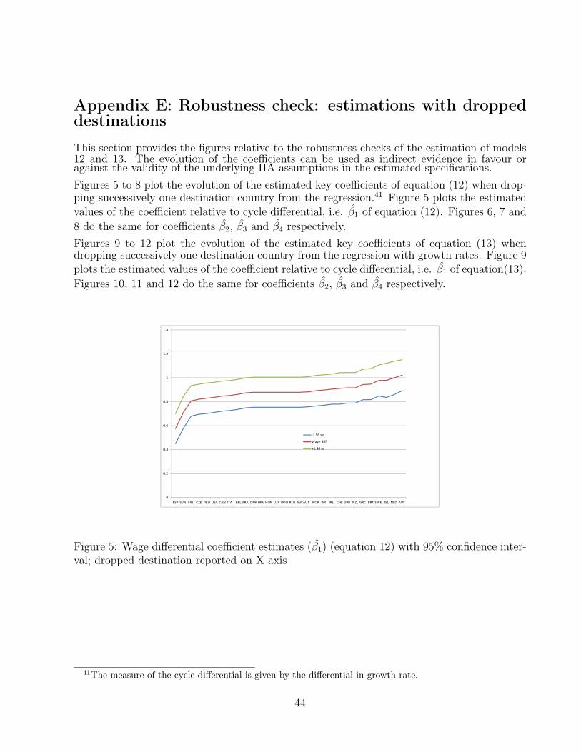
Appendix E: Robustness check: estimations with droppeddestinations

This section provides the figures relative to the robustness checks of the estimation of models12 and 13. The evolution of the coefficients can be used as indirect evidence in favour oragainst the validity of the underlying IIA assumptions in the estimated specifications.Figures 5 to 8 plot the evolution of the estimated key coefficients of equation (12) when drop-ping successively one destination country from the regression.41 Figure 5 plots the estimatedvalues of the coefficient relative to cycle differential, i.e. β̂1 of equation (12). Figures 6, 7 and8 do the same for coefficients β̂2, β̂3 and β̂4 respectively.Figures 9 to 12 plot the evolution of the estimated key coefficients of equation (13) whendropping successively one destination country from the regression with growth rates. Figure 9plots the estimated values of the coefficient relative to cycle differential, i.e. β̂1 of equation(13).Figures 10, 11 and 12 do the same for coefficients β̂2, β̂3 and β̂4 respectively.

0 6

0.8

1

1.2

1.4

0

0.2

0.4

0.6

ESP SVN FIN CZE DEU USA CAN ITA BEL FRA DNK HRV HUN LUX ROU RUS SVK AUT NOR ISR IRL CHE GBR NZL GRC PRT SWE ISL NLD AUS

‐1.96 se

Wage diff

+1.96 se

Figure 5: Wage differential coefficient estimates (β̂1) (equation 12) with 95% confidence inter-val; dropped destination reported on X axis

41The measure of the cycle differential is given by the differential in growth rate.

44

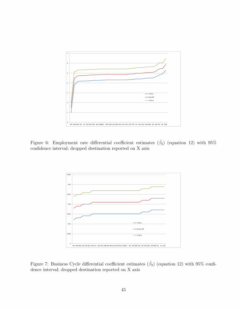
3

4

5

6

7

0

1

2

3

ESP DEU NOR ISR ISL SVN NLD GRC BEL DNKAUT HRV HUN LUX ROU RUS SVK FRA CHE PRT ITA NZL AUS USA GBR CZE CAN FIN IRL SWE

‐1.96 se

empl diff

+1.96 se

Figure 6: Employment rate differential coefficient estimates (β̂2) (equation 12) with 95%confidence interval; dropped destination reported on X axis

0.015

0.02

0.025

0.03

0.035

0

0.005

0.01

0.015

FIN SVN SWE USA PRT NLD CAN ITA BEL FRA DNKHRV HUN LUX ROU RUS SVK AUT ISR CHE GBR NZL CZE DEUGRC ESP NOR IRL ISL AUS

‐1.96 se

Growth diff

+1.96 se

Figure 7: Business Cycle differential coefficient estimates (β̂3) (equation 12) with 95% confi-dence interval; dropped destination reported on X axis

45

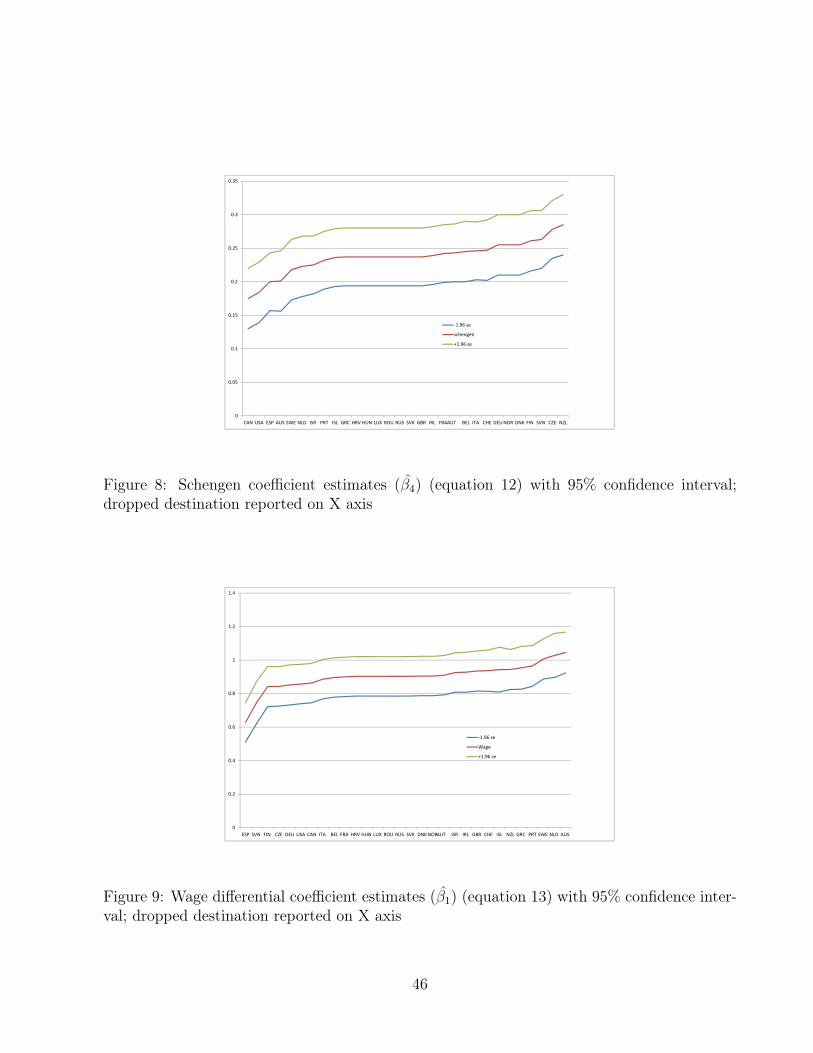
0.15

0.2

0.25

0.3

0.35

0

0.05

0.1

0.15

CAN USA ESP AUS SWE NLD ISR PRT ISL GRC HRV HUN LUX ROU RUS SVK GBR IRL FRA AUT BEL ITA CHE DEUNOR DNK FIN SVN CZE NZL

‐1.96 se

schengen

+1.96 se

Figure 8: Schengen coefficient estimates (β̂4) (equation 12) with 95% confidence interval;dropped destination reported on X axis

0.6

0.8

1

1.2

1.4

0

0.2

0.4

0.6

ESP SVN FIN CZE DEU USA CAN ITA BEL FRA HRV HUN LUX ROU RUS SVK DNKNOR AUT ISR IRL GBR CHE ISL NZL GRC PRT SWE NLD AUS

‐1.96 se

Wage

+1.96 se

Figure 9: Wage differential coefficient estimates (β̂1) (equation 13) with 95% confidence inter-val; dropped destination reported on X axis

46

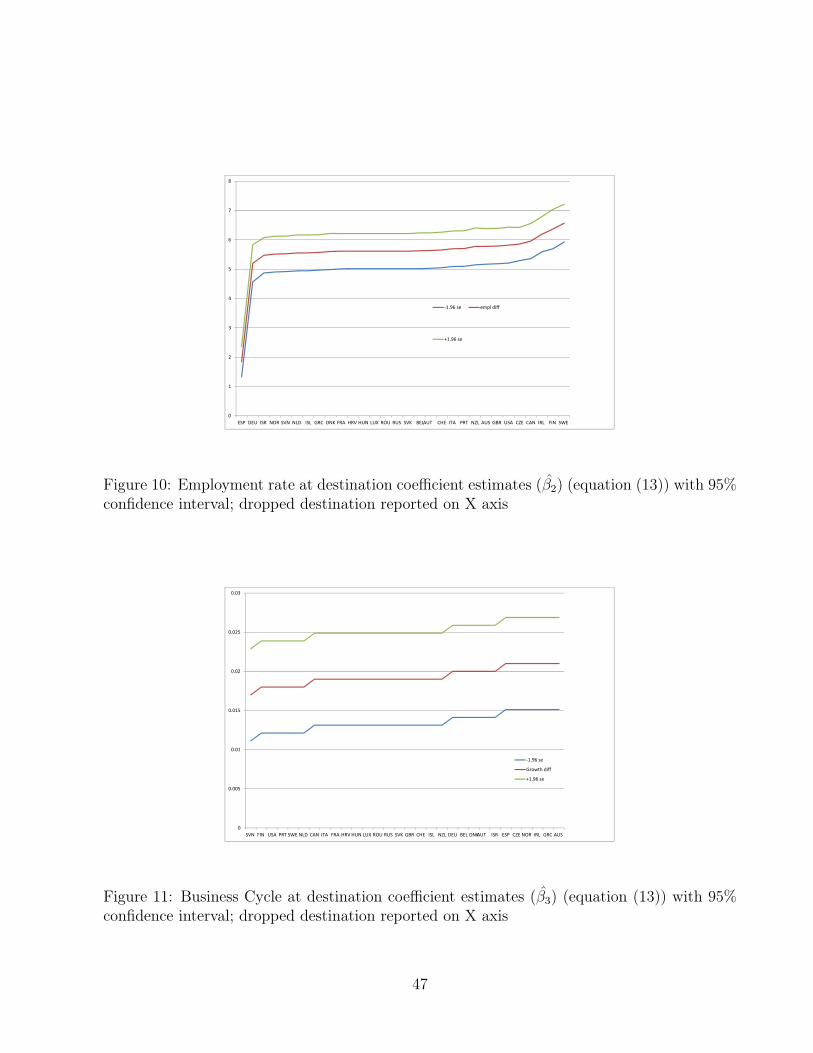
4

5

6

7

8

‐1.96 se empl diff

0

1

2

3

ESP DEU ISR NOR SVN NLD ISL GRC DNK FRA HRV HUN LUX ROU RUS SVK BELAUT CHE ITA PRT NZL AUS GBR USA CZE CAN IRL FIN SWE

+1.96 se

Figure 10: Employment rate at destination coefficient estimates (β̂2) (equation (13)) with 95%confidence interval; dropped destination reported on X axis

0.015

0.02

0.025

0.03

0

0.005

0.01

SVN FIN USA PRT SWE NLD CAN ITA FRA HRV HUN LUX ROU RUS SVK GBR CHE ISL NZL DEU BEL DNKAUT ISR ESP CZE NOR IRL GRC AUS

‐1.96 se

Growth diff

+1.96 se

Figure 11: Business Cycle at destination coefficient estimates (β̂3) (equation (13)) with 95%confidence interval; dropped destination reported on X axis

47

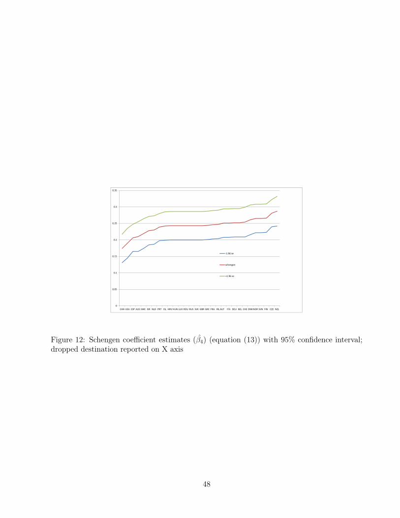
0.15

0.2

0.25

0.3

0.35

‐1.96 se

0

0.05

0.1

0.15

CAN USA ESP AUS SWE ISR NLD PRT ISL HRV HUN LUX ROU RUS SVK GBR GRC FRA IRL AUT ITA DEU BEL CHE DNKNOR SVN FIN CZE NZL

schengen

+1.96 se

Figure 12: Schengen coefficient estimates (β̂4) (equation (13)) with 95% confidence interval;dropped destination reported on X axis

48