Trade and the Diffusion of the Industrial

Revolution

Robert E. Lucas, Jr.∗

The University of Chicago

July, 2007

∗This paper is a version of the Frank D. Graham Memorial Lecture, which I gave at Princeton

in March, 2007. I thank Nancy Stokey, Sam Kortum, Gene Grossman, and Esteban Rossi-Hansberg

for their comments.

1

1. Introduction

The industrial revolution–the modern era of sustained growth in living standards–

has been underway in the most successful societies for more than two centuries. This

event followed centuries over which the annual incomes of ordinary working people

remained within a range of, say, $500-$800 (in today’s U.S. prices). Growth rates

in the leading economies have remained close two percent percent per year since the

19th century. Over two centuries, this adds up to a more than 40-fold increase in

GDP per capita. Since some countries have remained at or near Malthusian income

levels, this growth has given rise to an enormous and historically unprecedented level

of cross-country inequality.

In such a context, a study of economic growth in the world as a whole must be

a study of the diffusion of the industrial revolution across economies, a study of the

cross-country flows of production-related knowledge from the successful economies to

the unsuccessful ones. These flows are the main force for the reduction of income

inequality, for the convergence of incomes to a common, growing level. In this paper

I will show that these flows, when unimpeded by what Parente and Prescott (2002)

call “barriers to riches,” follow simple laws that can be described with a few para-

meters, parameters that have remained stable over time and can be estimated with

some accuracy from historical data. In carrying out this program, I use an empirical

definition of what it means for an economy to be “unimpeded” or “open,” based on

the work of Sachs and Warner (1995) and make use of the large body of evidence

on countries that have successfully made the transition from stagnation to sustained

growth.

The model itself is a modified version of the model I used in Lucas (1993, 2000),

closely related to Rodriguez (2006), and based on the earlier work of Tamura (1991)

and Barro and Sala-i-Martin (1992). Section 2 reviews Sachs and Warner’s definition

2

of “openness” and uses the 1960-2000 GDP per capita data from the Maddison (2003)

data set to calibrate a “spillover” parameter that describes technology flows among all

but the poorest of the open economies. Section 3 shows that the same, one parameter

model describes the way the pace of early development has accelerated over the last

two centuries, as documented by Parente and Prescott (2000), also using Maddison’s

data.

The aim of this model-construction is to use the abundant evidence on economies

that have successfully industrialized to learn about the possibilities for the poor

economies that have only begun to do so, or those where growth has slowed after

promising beginnings. But the model of Section 2 does not describe the growth be-

havior of the predominantly agricultural economies of Southeast Asia, even when they

have pursued open economic policies. Section 4 introduces a traditional agriculture

sector into the spillover model, in a way that is consistent with evidence on the differ-

ential effects of technology flows on agricultural production and production in other

sectors. Section 5 adds a third parameter to capture possible “agglomeration” effects

of concentrating people in the urban, non-agricultural sector. Section 6 applies the

model, so elaborated, to the very different experiences of four open Asian economies:

South Korea, Hong Kong, Thailand, and Indonesia. Section 7 contains concluding

remarks.

2. Post-1960 Evidence

The end of European colonial age in the 1960s gave rise to a host of new nations,

creating an invaluable laboratory for the study of comparative economic performance.

Figure 1 plots the average, annual growth rates of per capita production (real GDP)

over the 40 years 1960-2000 against the 1960 per capita GDP levels for 112 countries.

The data are taken from Maddison (2003). I have avoided labelling the countries on

the figure in an attempt to resist anecdotal digressions, but any regular reader of the

3

Economist will recognize many of them and come close to the rest. The triangular

pattern in this scatter is familiar to students of growth. The rich countries–mainly

Europe, North America, and Japan–all have growth rates close to two percent.

The poorest countries–mainly Africa and Asia–show extreme variety in growth

rates, ranging from the miraculous growth of South Korea, Taiwan, Hong Kong and

Singapore to the stagnation and even negative growth of some African and Asian

countries.

In their 1995 paper, Sachs and Warner classified all the countries on Figure 1 into

open and closed economies, based on a country-by-country survey of trade and other

policies over the period 1970-1990. I applied the Sachs-Warner classification to the

entire 1960-2000 period. Figure 2 repeats Figure 1 with the economies classified as

open indicated by solid dots and the closed economies by circles. One is struck by the

fact that most of the open economies line up on the line that forms the upper edge of

the triangle. I want to develop the idea that this line represents the possibilities for

economic growth that were available to any economy over the 1960-2000 period under

the economic policies that Sachs and Warner summarize in the term “openness.” (It

is clear from Figure 2 that this hypothesis does not quite work for all of the open

countries that were poorest in 1960: This exception is important, and I will come

back to it later on.)

Sachs and Warner are explicit about the definition of openness they use, but it is

a complicated one. To be classed as open, an economy must pass five tests. It must

(1) have effective protection rates less than 40 percent, (2) have quotas on less than

40 percent of imports, (3) have no currency controls or black markets in currency, (4)

have no export marketing boards, and (5) not be socialist (using the Kornai (1992)

definition). Clearly these standards do not hold an economy to a Smithian ideal of

laissez faire: There is plenty of room for Japanese or Korean mercantilism. The

4

0 2000 4000 6000 8000 10000 12000 14000-0.04

-0.02

0

0.02

0.04

0.06

FIGURE 1 : INCOME AND GROWTH RATES, 112 COUNTRIES

1960 Per Capita Income (1990 $)

Ann

ual G

row

th R

ate,

196

0-20

00

0 2000 4000 6000 8000 10000 12000 14000-0.04

-0.02

0

0.02

0.04

0.06

FIGURE 2 : INCOME AND GROWTH RATES, 112 COUNTRIES

1960 Per Capita Income (1990 $)

Ann

ual G

row

th R

ate,

196

0-20

00

= open= closed

currency control test is, I think, just a way of tagging governments that cannot keep

their hands to themselves. The export marketing boards are an African device (carried

over from colonial times) requiring farmers to sell export crops to the government

at a low price set by the latter, which then resells them abroad at world prices.

Kornai’s “socialist” countries are the communist dictatorships. The focus of the

Sachs-Warner classification is thus on the abilities of individuals to engage fairly

freely in international trade. High trade volumes–think of the oil exporters or barter

deals within the old Soviet bloc–are not accepted as proof of openness.1

Sachs and Warner provide a detailed, country-by-country appendix describing the

way their criteria are applied over the 20 year period their study covers. An evident

limitation of their definition of openness is its zero-one character: A country is labelled

either open or closed for the entire period. The problems this raises are even more

serious in my application, which covers the 40 year period up to 2000. Thus my Figure

2 classifies all of Eastern Europe as closed, even though must of these countries opened

after 1990 and many are now members of the European Union. Many other countries

have undertaken major policy reforms. A replication that reclassifies all the countries

based on the criteria (1)-(5) to the entire period would be an important improvement.2

There is controversy over whether the superior growth performance of the countries

classified as open by Sachs andWarner arises from differences in trade policies or from

other factors. This is unavoidable. Figure 3 breaks out 25 European countries, open

and closed, from Figure 2. The open economies are simply western Europe; the closed

ones are the former communist countries of eastern Europe. The information in the

1McGrattan and Prescott (2007) propose a definition of “openness” based on receptivity to foreign

direct investment. It would be useful to incorporate this criterion into the Sach-Warner classification

scheme, but my guess is that few countries would be re-classified if this were done.2See Wazciarg and Welch (2003) for an interesting follow-up paper that also uses post-1990

evidence, and exploits the panel character of the data set to examine the growth effects of within-

period changes in trade policies.

6

figure is not enough to let us separate the effects of trade policy from the effects of

central planning, followed in many countries by the chaotic transitions of the 1990s.

The other striking feature of Figure 3 is the regularity of the behavior of the open,

western economies. These points on the graph trace out a downward sloping curve

that illustrates the equalizing forces operating within the set of market economies.

The poorer a western European country was in 1960, the faster it grew between

1960 and 2000. This equalizing, which could have taken place in the first half of the

century but did not, is widely attributed to the formation and gradual expansion of

the European Union over these 40 years.3 Morever, going back to Figure 2, we can see

that a curve fit to the open Europeans will also fit the fast growing Asian economies.

In order to interpret and quantify this relation, I will use a mechanical model of

catch-up growth based on technology spillovers.4 We consider a world of one-sector

“AK” economies in which an economy’s GDP per capita is proportional to its stock

of human capital, or knowledge capital, or whatever term you like. There is a leading

economy or group of economies in which this stock of knowledge follows

H(t) = H0eµt. (1)

The stock of any other, poorer, economy follows

dh

dt= µh1−θHθ. (2)

In terms of GDP growth rates, these equations imply that the leader grows at a

constant rate µ while a follower grows at the rate

µ

µH

h

¶θ

.

3Ben David (1993) documented the role of the EEC in equalizing incomes among the original

six members. His conclusions would certainly be strengthened by including Spain and other later

entrants.4See Tamura (1991), Lucas (1993), Rodriguez (2006).

7

Since H > h, the follower grows faster than the leader, at a rate that depends on the

size of the GDP gap, H/h, and the size of the spillover parameter, θ. I want to see

how well a constant-θ model fits the evidence on open economies in Figures 2 and 3,

and find the particular θ value that fits best.

The solution to the differential equation for h(t) is

h(t) = H0eµt£1− (1− z0) e

−µθt¤1/θ (3)

where z0 = (h0/H0)θ . To use this solution to interpret the Sachs-Warner plots, we

write the implied average growth rate over a T year period as

g =1

T[log(h(T, h0))− log(h0)] ,

where h0 is (proportional to) per capita GDP at the beginning of the period. The

figures to follow plot g against h0, using the values µ = .02, T = 40, H0 = 12, 000,

and various θ values as indicated.

Figure 4 fits this curve to the western European data, using the spillover parameter

θ = 0.67. Figure 5 fits the same curve to all 39 open economies. Figure 6 indicates

that θ values ranging from 0.5 to 0.83 will fit this evidence about as well as the

value 0.67. The U.S. and Canada, Australia, and New Zealand fall more or less

right on the European curve, as do the fast-growing Asian economies: Japan, South

Korea, Taiwan, Hong Kong, and Singapore. It is worth repeating, though, that

many of the poorer, open Asian economies fall well below the curve, their openness

notwithstanding.

8

0 2000 4000 6000 8000 10000 12000 140000

0.01

0.02

0.03

0.04

0.05

0.06

0.07FIGURE 3 : 25 EUROPEAN COUNTRIES

1960 Per Capita Income (1990 $)

Ann

ual G

row

th R

ate,

196

0-20

00

-- western Europe-- eastern Europe

0 2000 4000 6000 8000 10000 12000 140000

0.01

0.02

0.03

0.04

0.05

0.06

0.07FIGURE 4 : 17 OPEN EUROPEAN COUNTRIES

1960 Per Capita Income (1990 $)

Ann

ual G

row

th R

ate,

196

0-20

00 Parameter Valuesθ = .67µ = .02

0 2000 4000 6000 8000 10000 12000 140000

0.01

0.02

0.03

0.04

0.05

0.06

0.07FIGURE 5 : 39 OPEN ECONOMIES

1960 Per Capita Income (1990 $)

Ann

ual G

row

th R

ate,

196

0-20

00 Parameter Valuesθ = .67µ = .02

0 2000 4000 6000 8000 10000 12000 140000

0.01

0.02

0.03

0.04

0.05

0.06

0.07FIGURE 6 : 39 OPEN ECONOMIES

1960 Per Capita Income (1990 $)

Ann

ual G

row

th R

ate,

196

0-20

00 Parameter Valuesθ = .5, .67, .83µ = .02

To sum up, I interpret the 1960-2000 evidence on comparative production and

growth as consistent with the hypothesis that an open economy, in the sense of Sachs

and Warner, will have an income growth path described by equations (1) and (2). If

so, the growth rate of per capita GDP in an open economy is equal to

.02×µH

h

¶2/3,

where H/h is the ratio of U.S. GDP to the home economy’s. For Poland or Uruguay

or Mexico, for example, where per capita GDP is something like 0.3 times the U.S.

level, this implies a potential growth rate of about 4.5 percent.5

3. Post-1820 Evidence

The Industrial Revolution did not begin in 1960. It began in Britain in the 18th

century and was spreading rapidly to other European countries by the early 19th

century. If this diffusion model I have applied to the postwar period is accurate, it

should be consistent with evidence from the 200 years prior to 1960 as well. To see

if this is so, I will use Figure 7, taken from Parente and Prescott (2002). The figure

is based on Maddison’s data for 50 countries in which per capita GDP had reached

$4000 (1990 U.S.) by 1990. Each point on the figure plots the number of years it took

for that country’s income to grow from $2000 to $4000 against the date that country

reached $2000. As one can see from the figure, the early leaders in industrialization

(the U.K, the Netherlands) needed over 50 years for income to double from 2000 to

4000. Countries that only reached 2000 after 1950 needed from 10 to 20 years.

This finding is clearly consistent qualitatively with the model (1) and (2). To check

the quantitative performance of the model, we use the same solution (3) to calculate

5This usage has the limitation that a country may exceed its “potential” even over long periods

and it is easy to think of specific cases where this has occurred.

11

the prediction

D =hθ(t+D)− hθ(t)

µθHθ(t)= ke−µθt,

where k is a constant to be determined, for the relation between a country’s doubling

time D and the date t when 2000 was reached. I used µ = .02 to draw these curves,

and tried different values for k and the spillover parameter θ. To my eye, θ = 0.5

gives the best fit, but from Figure 8 one can see that the long term data are about

as well described using the postwar estimate of θ = .67.

The graphical displays of Sachs and Warner and Parente and Prescott are com-

pletely different in their construction. Sachs and Warner’s is based on a painstaking

classification of countries based on a specific definition of their openness. In my

calibration, all the evidence from countries classified as closed is simply discarded.

Parente and Prescott do not mention openness in connection with their figure, and

indeed do not explain their 2000/4000 selection criterion at all. But in practice

the two selection procedures have similar effects. Excluding countries that had not

reached the 4000 level of income by 1990 rules out all of Africa and the large Asian

economies, nearly all of which are also closed according to Sachs and Warner. Parente

and Prescott’s neglect of evidence on countries’ growth performance after passing 4000

excludes the poor postwar performance of eastern Europe and Latin America, areas

that were economically similar to southern Europe until the 1930s and the postwar

years. These countries, too, are closed by the Sachs-Warner criteria.

In my interpretation of this evidence, the theoretical model is understood as a

description of potential economic growth, and shortfalls from this potential are im-

plicitly treated as the result of bad policies, wars, and the like. I have not spelled out

the details of these exceptions and do not intend to do so here, but it is fair to ask

how tenable this view is as a working hypothesis. With respect to eastern Europe

and Latin America, I find it very plausible. Certainly I share the widely held view

that the poor postwar economic performance of eastern Europe can be attributed to

12

1820 1840 1860 1880 1900 1920 1940 1960 19800

10

20

30

40

50

60

70

80FIGURE 7: INCOME DOUBLING TIMES, 50 COUNTRIES

Year income reached 2000 (1990 U.S. $)

Yea

rs fo

r inc

ome

to d

oubl

e to

400

0

Source: Parente and PrescottBarriers to RichesTable A.1, pp. 31-32

1820 1840 1860 1880 1900 1920 1940 1960 19800

10

20

30

40

50

60

70

80FIGURE 8: INCOME DOUBLING TIMES, 50 COUNTRIES

Year income reached 2000 (1990 U.S. $)

Yea

rs fo

r inc

ome

to d

oubl

e to

400

0

Parameter Values:µ = .02θ = 0.3, 0.5, 0.7

the deficiencies of socialist central planning. For Latin America, Figure 9 contrasts

the postwar economic growth of southern Europe (solid lines) and the four Latin

American countries that are largely populated by southern European peoples (dashed

lines). These culturally similar societies had similar income levels in 1950. Since

1950, the southern Europeans have joined in, and contributed to, the prosperity of the

European union. With the exception of Chile, the south Americans have continued to

follow the protectionist policies of the interwar years. The two groups have steadily

diverged (and Chile is now the richest of the four Americans). The figure is only

suggestive, but it is surely plausible that, as is the case with eastern Europe, the poor

economic performance of Latin America is a policy-induced failure to reach economic

potential and does not indicate any deficiency in the model (1)-(3) as a description

of potential growth.

For the poor economies of Asia and Africa, in contrast, the diffusion model needs

basic modification, even as as description of an ideal of behavior. Figure 10 isolates

the open Asian economies from Figure 2, including Japan, South Korea, and the

overseas Chinese. (Mainland China is, of course, closed under the Sachs-Warner

criteria.) But there are four relatively slow growing exceptions, labelled on the figure,

also classed as open. All four were very poor in 1960, and in common with all other

very poor economies, their labor force was mainly engaged in traditional agriculture.

Compared with the rest of Asia and Africa the economic performance of these open

exceptions was well above average–see Figure 2–but their growth rates were far

below the curve I have tentatively proposed to describe potential growth.

This should be no surprise. The formula g = θ(H/h) implies that as h → 0,

given the position H of the leader, potential growth becomes infinite. The very

poorest countries should have the highest growth rates. But who, in these poor,

largely illiterate feudal societies is available to absorb and internalize this inflow of

new technology, even under the best economic policies? In effect, equations (1)-(3)

14

1950 1955 1960 1965 1970 1975 1980 1985 1990 1995 20000

2

4

6

8

10

12

14

16

18

20FIGURE 9: SOUTHERN CONE AND SOUTHERN EUROPE

GD

P P

ER

CA

PIT

A, T

HO

US

AN

DS

OF

1990

DO

LLA

RS Dashed lines: Argentina, Brazil, Chile, Uruguay

Solid lines: Italy, Spain, Portugal

0 2000 4000 6000 8000 10000 12000 140000

0.01

0.02

0.03

0.04

0.05

0.06

0.07FIGURE 10: 16 ASIAN COUNTRIES

1960 Per Capita Income (1990 $)

Ann

ual G

row

th R

ate,

196

0-20

00

Indonesia

Sri Lanka

Malaysia

Thailand

-- open

-- closed

represent an attempt to model the flow of ideas without taking into account the

ability of recipients to absorb and make productive use of these ideas.

4. A Dual Economy Model

In order to construct a model that is capable of describing the growth possibilities

open to poor economies, we would like to have a direct measure of an economy’s ability

to absorb technology, to participate in the conversations that technology transfer

requires. Certainly comparative schooling levels are important, observable, and much

studied. I will focus here, however, on an indirect but related measure: the fraction

of an economy’s employment that is in agriculture. The idea is certainly not that

human capital is not useful in agriculture–we have much evidence to the contrary

from the advanced economies–but that in poor economies with a high fraction of

employment in agriculture, the agricultural sector tends to be low skilled. Schultz

(1964) used the term traditional agriculture for farm technologies carried over from

the feudal era, many of which are still in use in poor countries today. Migration out

of traditional agriculture is a central element of growth, both as a consequence and,

I believe, as a cause.

Empirically, the share of agriculture in employment has a systematic connection

to GDP per capita. We will see this in a 1980 cross-section of countries. It can also

be seen in long time series, using selected countries from Kuznets (1971). Figure 11

plots the share of employment in agriculture against an economy’s per capita GDP

(in logs), for 112 countries. The wealthy economies all have shares under 10%, the

poorest as high as 90%. For employment, I used the 1984 World Development Report;

for real income, I used Maddison.

In Figure 12, I plotted the time paths of employment shares for four countries,

using Kuznets (1971), Table 21, plus the 2004 Pocket World in Figures put out by

the Economist magazine. By the early 19th century, much of the U.K.’s migration

17

5.5 6 6.5 7 7.5 8 8.5 9 9.5 10 10.50

10

20

30

40

50

60

70

80

90

100FIGURE 11: AGRICULTURAL EMPLOYMENT SHARES, 1980

LOG PER CAPITA GDP, 1990 DOLLARS

EM

PLO

YM

EN

T S

HA

RE

OF

AG

RIC

ULT

UR

E

112 COUNTRIES

1800 1820 1840 1860 1880 1900 1920 1940 1960 1980 20000

10

20

30

40

50

60

70

80

90FIGURE 12: EMPLOYMENT SHARES IN AGRICULTURE

EM

PLO

YM

EN

T S

HA

RE

, PE

RC

EN

T

U.K.

U.S.

Japan

India

6 6.5 7 7.5 8 8.5 9 9.5 10 10.50

10

20

30

40

50

60

70

80

90FIGURE 13: EMPLOYMENT SHARES IN AGRICULTURE

LOG PER CAPITA GDP

EM

PLO

YM

EN

T S

HA

RE

, PE

RC

EN

T

U.K.

U.S.Japan

India

out of agriculture had already taken place. The other three were then still predom-

inantly agricultuiral, as India is today.

To compare the historical evidence to the 1980 cross section, I used Maddison’s

data for years chosen to correspond as closely as possible to Kuznets’ and plotted the

agricultural employment shares against the log of GDP rather than time. This plot

is shown in Figure 13.

To interpret this evidence and summarize it in an analytically useful way, I will

use a two sector, “dual economy” model. Call the two sectors “farm” and “city.” A

fraction 1 − x of each unit of labor in the economy is allocated to the city sector,

where it produces

yc = h(1− x).

Here h denotes the economy’s knowledge level, as in the earlier model. The remaining

fraction x is allocated to the farm sector, where it produces

yf = Ahξxα

units of the same, single output good. Here land per person is taken as fixed and in-

corporated into the intercept A. The parameter ξ will be calibrated using the evidence

in Figures 12 and 13; it cannot be taken equal to 0 to fit this evidence. I interpret ξ

as reflecting a spillover effect of city knowledge on agricultural productivity.6

Following Hansen and Prescott (2002), I assume that labor is mobile so that the

equilibrium and optimal allocations x coincide. There is a good case that migration

to the city requires human capital accumulation (before or just after the move). This

6By assuming a single output good, I am neglecting the effects of a low income elasticity of food

demand in accounting for the relative slow growth of the agricultural sector. This low elasticity

plays an important role in the accounts of the British industrial revolution of Laitner (2000) and

Stokey (2001). See Shin (1990) for a careful atempt to identify the separate effects of differential

technological change (which I emphasize) and the low income elasticity, using U.S. and Korean time

series. He finds that both effects are important.

19

possibility is emphasized in Lucas (2004). There may be other barriers or costs to

migration as well. But let us see what we can learn from the mobile labor model.

In this case, equilibrium output is given by

y(h) = maxx

£Ahξxα + h(1− x)

¤. (4)

If

αAhξxα−1 > h

then x = 1. Otherwise x is given by

x(h) =

µαA

h1−ξ

¶1/(1−α). (5)

When h → ∞, as will be the case for any industrializing economy, x(h) → 0: The

traditional agriculture sector eventually empties out.

The two functions, x(h) and y(h) defined by this model have implications for the

way the employment share in agriculture should vary with GDP per capita. Evi-

dence on this relation can provide information on the parameter ξ. In Figure 14, the

theoretical curve (y(h), x(h)) implied by (4) and (5) is superimposed on the 1980

cross-section plot. I used the labor share parameter α = 0.6 and chose the intercept

A and the spillover parameter ξ = 0.75 to get the figure shown. Figure 15 uses the

same model with the same parameter values to fit the time series evidence from four

countries. The cross-section and time-series evidence agree completely: Both indicate

that a 10 percent increase in non-farm productivity is associated with a 7.5 percent

increase in farm productivity.

20

5.5 6 6.5 7 7.5 8 8.5 9 9.5 10 10.50

10

20

30

40

50

60

70

80

90

100FIGURE 14: AGRICULTURAL EMPLOYMENT SHARES, 1980

112 COUNTRIES

LOG PER CAPITA GDP

EM

PLO

YM

EN

T S

HA

RE

OF

AG

RIC

ULT

UR

E

Parameter Values:α = 0.6ξ = 0.75

5.5 6 6.5 7 7.5 8 8.5 9 9.5 10 10.50

10

20

30

40

50

60

70

80

90

100FIGURE 15: EMPLOYMENT SHARES IN AGRICULTURE

LOG PER CAPITA GDP

EM

PLO

YM

EN

T S

HA

RE

, PE

RC

EN

T

U.K.

U.S.Japan

India

Parameter Values:α = 0.6ξ = 0.75

5. Dual Economy Dynamics

The use of the dual economy model to estimate the parameter ξ was a static

exercise. Now we reintroduce some dynamics. One way to do this would be to repeat

the formula (2), but this would not solve the problem that led us to formulate a dual

economy model in the first place. The intention was to incorporate the economies

dominated by traditional agriculture into the model by adding a feature that slows

down the transmission of technology to these economies. With ξ < 1, the agriculture

sector does act as a drag, but not a large enough one to reverse the prediction of

unrealistically high growth rates in very poor, open economies..

We need to add a second feature, focusing on the role of cities as centers of intel-

lectual interchange, as the recipients of technological inflows. Scale or agglomeration

effects are central to this role.7 I will treat these as external effects, and modify (2)

to the formdh

dt= µ [1− x(h)]ς h1−θHθ. (6)

Think of the new term [1− x(h)]ς as a kind of agglomeration effect, according to

which the rate of technology inflow to any individual is an increasing function of the

city population. Why the fraction of people in the city, as opposed simply to the

number? Because large scale economies at the economy-wide level are untenable.8

Combining (5) and (6) yields a modified model

dh

dt= µ

"1−

µαA

h1−ξ

¶1/(1−α)#ςh1−θHθ, (7)

provided the expression in brackets is positive. (Otherwise, knowledge growth is zero

and the economy never industrializes.) If the knowledge level h is large enough to

7See, for example, Baldwin and Martin (2006) and references therein.8See Henderson and Ioannides (1981) and, in a context closer to this analysis, Rossi-Hansberg

and Wright (2007) for models in which countries with large populations have more cities, but not

larger cities, than do small countries.

22

induce any growth, then (7) implies that h will grow forever. The added agglomer-

ation or urban spillover term will approach one (whatever the value of the positive

parameter ζ) and the economy will ultimately behave exactly as in the model (1)-(3):

Both the level of GDP and the growth rate will approach the values of the leading

economy.

For small values of h, however, the growth rate of h approaches zero. The modi-

fication of the model was designed to eliminate the growth “advantage” of extreme

poverty and it achieves this in what I think is a realistic way. As we will see, the para-

meter ζ can be chosen to give good quantitative agreement to the growth performance

of predominantly agricultural economies.

The solution to (7) cannot be written out as a formula like (3), but it can be solved

numerically. Given initial values H(0) and h(0) for the rich and poor economies, (2)

and (7) give paths for H(t) and h(t). Given these solutions, we can get the labor

allocation x(h) and per capita GDP y(h) from (4) and (5). We know where these

variables are headed in the long run but we want to understand how they get there,

and how these dynamics depend on the added parameter ζ.

In the simulations reported next, the model is parameterized as follows. The be-

havior of the leading, rich economy is described by its constant growth rate µ = .02

and an initial H0 of 12000 1990 dollars (as in Figures 3-6). For all simulations, I set

labor’s share in farm production equal to α = 0.6. The technology spillover parameter

was set at θ = .65, consistent with the Sachs-Warner and Parente-Prescott evidence.

The city/farm spillover parameter was set at ξ = 0.75, consistent with the Kuznets

and World Bank evidence on employment shares in agriculture.

The local city spillover parameter ζ was added to the model because, without it,

the theory predicts unrealistically high growth rates for the poorest economies. There

is no information on these economies in the Parente-Prescott diagram, which has a

$4000 entry cost. The only information in the Sachs-Warner figures that potentially

23

bear on the value of ζ are the observations on the four predominantly agricultural

Asian economies highlighted in Figure 10. Accordingly I experimented with different

values of ζ using the initial values y0 = 830 for per capita GDP and x0 = 0.8 for the

employment share of agriculture, numbers which approximately describe Indonesia

or Thailand in 1960. I used these values to calibrate the agricultural production

intercept A and the initial human capital h0 of a fictional home economy. Figures

16 and 17 illustrate the behavior of this economy for the values ζ = 0, 1, 2, and 3 of

the local spillover parameter.

One can see that at ζ = 0 the initial growth rate is unrealistically high. (In

the simulation shown on Figure 16, it is 11 percent in the initial year.) As ζ is

increased (as local externalities become stronger) the country’s growth “miracle” is

postponed. Postponement implies a bigger miracle when in happens, due to the larger

technology gap. The migration from agriculture and the convergence of income levels

are postponed as well. In the rest of the simulations reported below, I will use the

value ζ = 1, which is roughly consistent with the average growth rates in Indonesia

or Thailand over the period 1960-2000.

The average growth rate of the ζ = 1 economy over the first 40 years is 4.4 percent,

but it is far from constant over these years. After five years of falling further behind

the leader, it undergoes something of a growth miracle, peaking at a rate just over

5 percent after 25 years. Thereafter, growth declines toward 2 percent forever. This

economy reaches $2000 per capita GDP level in year 24, and $4000 in year 38: a

doubling time of 14 years. It takes over 100 years for the GDP level to reach half of

the U.S. level, and after 200 years its relative income has reached 80%, comparable to

the relative positions of Europe or Japan today. Economic growth, even under ideal

conditions, is a slow process.

All of this behavior is pure economics: indeed, almost pure technology. The illus-

trated thought experiments hold policy fixed and “open.” The long run behavior

24

0 20 40 60 80 100 120 140 160 180 2000

0.01

0.02

0.03

0.04

0.05

0.06

0.07

0.08

0.09

0.1FIGURE 16: GDP GROWTH RATES, DIFFERENT ζ VALUES

AN

NU

AL

GR

OW

TH R

ATE

ζ = 0

ζ = 1 ζ = 2

ζ = 3

0 20 40 60 80 100 120 140 160 180 2000

0.1

0.2

0.3

0.4

0.5

0.6

0.7

0.8

0.9

1FIGURE 17: RELATIVE GDP, DIFFERENT ζ VALUES

GD

P P

ER

CA

PIT

A, R

ELA

TIV

E T

O U

S

ζ = 0

ζ = 1

ζ = 2ζ = 3

of the hypothetical economy is completely determined a priori, to be the same as the

long run behavior of U.S. There is a given initial technology gap; diffusion continues

until income equality is reached; annual growth rates converge to 2 percent. The only

unresolved questions are how long it will take, what the timing will be, and what will

be the peak growth rate.

6. Asian Growth: Four Case Studies

The modified theory (1) and (7) can accommodate some of the variety of experience

of the open Asian economies. For a given initial level of GDP, economies differ in

their observed initial fractions of employment in the farm sector, and in fact we

see that the fastest growing Asian economies had the smallest 1960 farm shares.

In my formulation of the dual economy model, x is not a second state variable so

such differences must be viewed as reflections of differences in the farm intercept

parameter A (or in some other parameter). That is to say, we can use the theory

to map an economy’s observed initial (x0, y0) pair into a pair (h0, A). The model

has the implication, noted by Matsuyama (1992) in a similar context, that high farm

productivity retards initial growth. In this section, I apply this idea to the 1960-2000

growth performance of four Asian economies: Hong Kong, South Korea, Indonesia,

and Thailand, all of which were classed as open by Sachs and Warner.

The data used to construct Figures 18-21 are Maddison’s estimates of real per

capita GDP for these four countries, plus World Bank data on the 1960 employment

shares of agriculture. The dotted lines on the figures are the actual 1960-2000 growth

rates. For all four Asian economies, these series are highly erratic compared to the

U.S. or Europe over this period. It is clear that the model I have developed here

has nothing to say about these high frequency movements. Acordingly, I used a

Hodrick-Prescott filter (with parameter 100), based on 1950-2000 data, to remove

high frequency components. The resulting smoothed series in each country are the

26

dashed lines on the figures. Finally, the smooth curve is the simulated series based

on each country’s initial pair (y0, x0). Let’s go through these in order.

In 1960, the Hong Kong GDP level was already at $2220 per person and the

fraction of employment in agriculture was only 8 percent. In the context of the

model, we interpret this combination as arising from a high (by 1960 Asian standards)

level of city human capital and (with obvious realism!) an extremely unproductive

agriculture. The dual economy elaborations of the basic model (1)-(3) thus contribute

nothing to explaining Hong Kong growth. Predicted growth rates decline steadily

from an initial peak level of 5.5 percent. This is the same model we would apply–

successfully–to postwar Spain, Italy, or Japan.

South Korea in 1960 was in a quite different situation, with a $770 income level

and 66 percent of employment in agriculture. The prediction of the model is that an

open economy in this situation such have a growth rate that increases from 4 percent

to nearly 6 percent in 15 years, and declines thereafter. Notice that actual growth in

both Hong Kong and South Korea was faster than “potential” growth as defined by

the model, especially so in Korea.

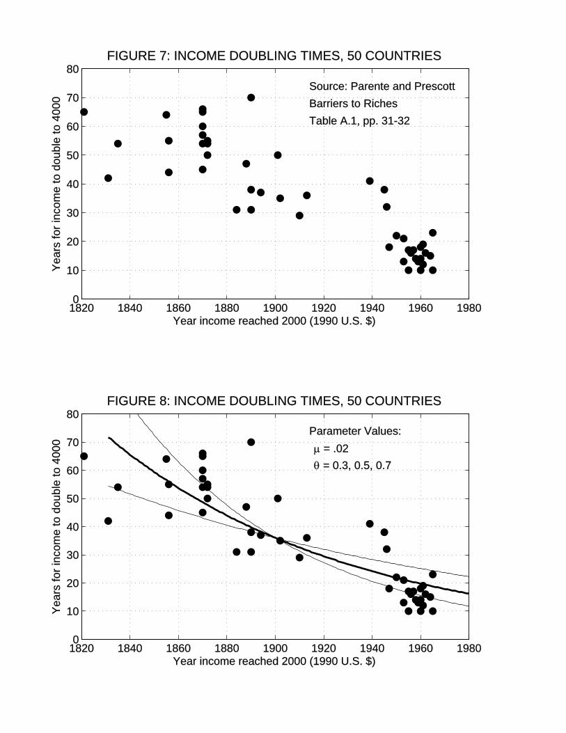
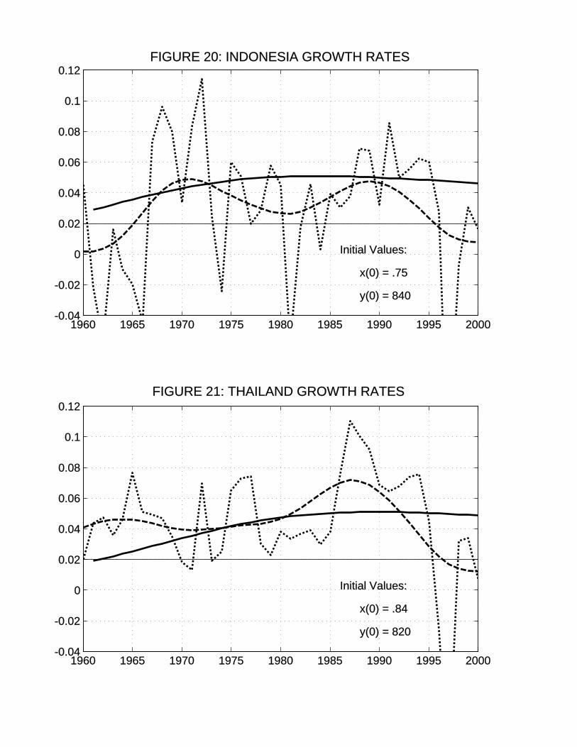
Figures 20 and 21 illustrate the economies of Indonesia and Thailand, both very

poor in 1960 and with very large agricultural sectors. In the model, these initial

conditions are interpreted as implying a relatively rich agricultural endowment, re-

tarding migration and hence growth for a time. Initial predicted growth in both is

near 2 percent in both, rising to 5 percent in 20 years in Indonesia and in 30 years in

Thailand.

I interpret these figures as a success for the dual economy model. The model

requires open economies to differ according to their initial human capital and their

agricultural wealth. These differences involve different rural-urban migration patterns

and different time patterns in growth rates. As compared to suitably smoothed actual

growth rate patterns, the predicted and actual behaviors look very similar. Of course,

27

1960 1965 1970 1975 1980 1985 1990 1995 2000-0.04

-0.02

0

0.02

0.04

0.06

0.08

0.1

0.12FIGURE 18: HONG KONG GROWTH RATES

Initial Values:

x(0) = .08

y(0) = 2220

1960 1965 1970 1975 1980 1985 1990 1995 2000-0.04

-0.02

0

0.02

0.04

0.06

0.08

0.1

0.12FIGURE 19: SOUTH KOREA GROWTH RATES

Initial Values:

x(0) = .66

y(0) = 770

1960 1965 1970 1975 1980 1985 1990 1995 2000-0.04

-0.02

0

0.02

0.04

0.06

0.08

0.1

0.12FIGURE 20: INDONESIA GROWTH RATES

Initial Values:

x(0) = .75

y(0) = 840

1960 1965 1970 1975 1980 1985 1990 1995 2000-0.04

-0.02

0

0.02

0.04

0.06

0.08

0.1

0.12FIGURE 21: THAILAND GROWTH RATES

Initial Values:

x(0) = .84

y(0) = 820

the theory does not contribute anything to our understanding of the high-frequency

movements in GDP and GDP growth rates. But thinking about political and financial

events in these four countries over the last 50 years will, I think, be more productive

if we can use economic theory to provide a benchmark of the economic growth that

would have occurred under conditions that are closer to “ideal.”

7. Concluding Remarks

The theory developed above has no explicit role for international trade, and the only

evidence on trade that I used was simply taken without modification from the Sachs-

Warner classication. But since I calibrated θ using data from the open economies only,

there is some logic in regarding reductions in the spillover parameter θ as representing

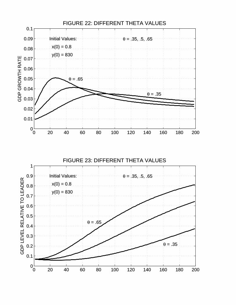
restrictive trade policies. Figures 22 and 33 describe simulations of otherwise identical

economies with θ values of 0.65 (representing openness) and 0.5 and 0.35 (representing

different deviations fron openness). The initial conditions resemble those of Thailand

and Indonesia in 1960. The most closed of these three economies reaches $2000 per

capita GDP level in year 85, and $4000 in year 109: a doubling time of 24 years. Its

average growth rate over the first 40 years is 7/10 of a percent.

These are enormous effects relative to available estimates of gains from trade.9

But they are computed under the assumption that trade restrictions are the only

explanation for poor growth performances. It would add credibility if one could use

economic theory and evidence to trace the quantitative connections of this spillover

parameter θ to specific trade policies, but this has not yet been done. Without this,

we cannot be sure what the “openness” measured by Sachs and Warner means, or

how much of observed growth rate differentials can be accounted for by differences in

openness.

I began this paper with Figure 1, an illustration of the enormous variety of economic

9See for example Alvarez and Lucas (2007) and other estimates cited there.

30

0 20 40 60 80 100 120 140 160 180 2000

0.01

0.02

0.03

0.04

0.05

0.06

0.07

0.08

0.09

0.1FIGURE 22: DIFFERENT THETA VALUES

GD

P G

RO

WTH

RA

TE

Initial Values:

x(0) = 0.8

y(0) = 830

θ = .35, .5, .65

θ = .65

θ = .35

0 20 40 60 80 100 120 140 160 180 2000

0.1

0.2

0.3

0.4

0.5

0.6

0.7

0.8

0.9

1FIGURE 23: DIFFERENT THETA VALUES

GD

P L

EV

EL

RE

LATI

VE

TO

LE

AD

ER

Initial Values:

x(0) = 0.8

y(0) = 830

θ = .35, .5, .65

θ = .35

θ = .65

performance observed in the post-World War II, post-colonial world. In part, as

everyone knows, this variety arose from wars, breakdowns of internal order, and mis-

guided ventures into centralized economic planning. But among the subset of coun-

tries that can be classed as predominantly “open,” a subset including countries that

were very rich in 1960 and some that were very poor, GDP levels and growth rates

can be well described by a very simple differential equation. This equation depends

on but five parameters, common to all economies, which can be estimated from avail-

able evidence, plus country-specific parameters describing land and other features

of agricultural endowments and the initial levels of countries’ productivities. Only

one of these parameters–the spillover parameter θ—plays an important role in the

growth behavior of economies that have reached, say, 25 percent of the current U.S.

per capita GDP level.

One can think of several economic forces beside trade policies that may have con-

tributed to the cross-country effects described by this parameter θ, including char-

itable transfers from rich to poor countries, lending by the rich to the poor, and

migration from poor to rich countries. But historically, direct transfers have been

neglible and the role of mortgaged capital flows has been minor. Migration has been

a very important force for equalization in the past (as it is for any species), but as

income gaps widened in the last century migration flows were drastically limited by

the wealthy countries. What is left but the flow of ideas, and how can idea flows not

be closed linked to the economic interactions involved in trade?

REFERENCES

[1] Alvarez, Fernando, and Robert E. Lucas, Jr. 2007. “General Equilibrium Analysis

of the Eaton-Kortum Model of International Trade.” Journal of Monetary Eco-

nomics, 54: forthcoming.

32

[2] Baldwin, Richard E. and Philippe Martin. 2006. “Agglomeration and Regional

Growth,” in J.Vernon Henderson and Jacques-Francois Thisse, eds., Handbook

of Regional and Urban Economics, vol. 4: Cities and Geography.

[3] Barro, Robert J., and Xavier Sala-i-Martin. 1992. “Technological Diffusion, Conver-

gence, and Growth.” Journal of Economic Growth, 2: 1-26.

[4] Ben David, Dan. 1993. “Equalizing Exchange: Trade Liberalization and Income Con-

vergence.” Quarterly Journal of Economics, 108: 653-679.

[5] Hansen, Gary D., and Edward C. Prescott. 2002. “Malthus to Solow.” American

Economic Review, 92: 1205-1217.

[6] Henderson, J. Vernon, and Yannis M. Ioannides. 1981. “Aspects of growth in a system

of cities.” Journal of Urban Economics, 10: 117-139.

[7] Kornai, Janos. 1992. The Socialist System: The Political Economy of Communism.

Princeton: Princeton University Press.

[8] Kuznets, Simon. 1971. Economic Growth of Nations: Total Output and Production

Structure. Cambridge: Harvard University Press.

[9] Laitner, John. 2000. “Structural Change and Economic Growth.” Review of Economic

Studies, 67: 545-561.

[10] Lucas, Robert E., Jr. 1993. “Making a Miracle.” Econometrica, 61: 251-272.

[11] Lucas, Robert E., Jr. 2000. “Some Macroeconomics for the 21st Century.” Journal of

Economic Perspectives, 14: 159-168.

[12] Lucas, Robert E., Jr. 2004. “Life Earnings and Rural-Urban Migration.” Journal of

Political Economy, 112: S29-S59.

33

[13] Maddison, Angus. 2003. The World Economy: Historical Statistics. Paris: OECD

Development Centre.

[14] Matsuyama, Kiminori. 1992. “Agricultural productivity, comparative advan-

tage, and economic growth.” Journal of Economic Theory, 58: 317-

334.

[15] McGrattan, Ellen, and Edward C. Prescott. 2007. “Openness, technology capital, and

development.” Federal Reserve Bank of Minneapolis Working Paper #651.

[16] Parente, Stephen L., and Edward C. Prescott. 2000. Barriers to Riches. Cambridge:

MIT Press.

[17] Rodriguez, Alejandro. 2006. “Learning Externalities, Human Capital and Growth.”

University of Chicago doctoral dissertation.

[18] Rossi-Hansberg, Esteban, and Mark L.J. Wright. 2007. “Urban Structure and

Growth.” Review of Economic Studies, 74: 597-624.

[19] Sachs, Jeffrey D. and Andrew Warner. 1995. “Economic Reform and the Process of

Global Integration.” Brookings Papers on Economic Activity, 1995: 1-118.

[20] Schultz, Theodore W. 1964. Transforming Traditional Agriculture. New Haven: Yale

University Press.

[21] Shin, Do Chull. 1990. “Economic Growth, Structural Transformation, and Agricul-

ture: The Cases of the United States and South Korea.” University of Chicago

doctoral dissertation.

[22] Stokey, Nancy L. 2001. “A Quantitative Model of the British Industrial Revolution,

1780-1850," Carnegie-Rochester Conference Series on Public Policy, 55: 55-109.

34

[23] Tamura, Robert. 1991. “Income Convergence is an Endogenous GrowthModel.” Jour-

nal of Political Economy, 99: 522-540.

[24] Wacziarg, Romain and Karen Horn Welch. 2003. “Trade Liberalization and Growth:

New Evidence.” NBER Working Paper No. 10152.

35