The Diffusion of Wal-Mart and Economies of Density

Thomas J. Holmes∗†

July 16, 2009

Abstract

The roll-out of Wal-Mart store openings followed a pattern that radiated from the center

outward with Wal-Mart maintaining high store density and a contiguous store network all

along the way. This paper estimates the benefits of such a strategy to Wal-Mart, focusing

on the savings in distribution costs afforded by a dense network of stores. The paper takes a

revealed preference approach, inferring the magnitude of density economies from how much

sales cannibalization of closely-packed stores Wal-Mart is willing to suffer to achieve density

economies. The model is dynamic with rich geographic detail on the locations of stores

and distribution centers. Given the enormous number of possible combinations of store-

opening sequences, it is difficult to directly solve Wal-Mart’s problem, making conventional

approaches infeasible. The moment inequality approach is used instead and it works well.

The estimates show the benefits to Wal-Mart of high store density are substantial and likely

extend significantly beyond savings in trucking costs.

∗University of Minnesota, Federal Reserve Bank, and the National Bureau of Economic Research.†The views expressed herein are solely those of the author and do not represent the views of the Federal

Reserve Banks of Minneapolis or the Federal Reserve System. I am grateful to for NSF Grant 0551062 for

support of this research. I have benefited from the comments of many seminar participants. In particular,

I thank Glenn Ellison, Gautam Gowrisankaran and Avi Goldfarb for their comments as discussants and

Kyoo-il Kim for comments and Ariel Pakes for advice on how to think about this problem. I thank Junichi

Suzuki, Julia Thornton Snider, David Molitor, and Ernest Berkas for research assistance. I thank Emek

Basker for sharing data.

1 Introduction

Wal-Mart opened its first store in 1962, and today there are over 3,000 Wal-Mart stores in

the United States. The roll-out of stores illustrated in Figure 1 displays a striking pattern.

(See also a movie of the roll-out posted on the web.1) Wal-Mart started in a relatively

central spot in the country (near Bentonville, Arkansas) and store openings radiated from

the inside out. Wal-Mart never jumped to some far off location to later fill in the area in

between. With the exception of store number one at the very beginning, Wal-Mart always

placed new stores close to where it already had store density.

This process was repeated in 1988 when Wal-Mart introduced the supercenter format.

(See Figure 2.) With this format, Wal-Mart added a full-line grocery store alongside the

general merchandise of a traditional Wal-Mart. Again, the diffusion of the supercenter

format began at the center and radiated from the inside out.

This paper estimates the benefits of such a strategy to Wal-Mart, focusing on the logis-

tic benefits afforded by a dense network of stores. Wal-Mart is vertically integrated into

distribution: general merchandise is supplied by Wal-Mart’s own regional distribution cen-

ters, groceries for supercenters through its own food distribution centers.2 When stores are

packed close together, it is easier to set up a distribution network that keeps stores close to

a distribution center. And when stores are close to a distribution center, Wal-Mart can save

on trucking costs. Moreover, such proximity allows Wal-Mart to respond quickly to demand

shocks. The ability of Wal-Mart to quickly respond to demand shocks is widely considered

to be a key aspect of the Wal-Mart model. (See Holmes (2001) and Ghemawat, Mark, and

Bradley (2004).) Wal-Mart famously was able to restock it shelves with American flags on

the very day of 9/11.

A challenge in estimating the benefits of density is that Wal-Mart is notorious for being

secretive–I cannot access confidential data on its logistics costs. So it is not possible to

conduct a direct analysis relating costs to density. And even if Wal-Mart were to cooperate

and make its data available, the benefits of being able to quickly respond to demand shocks

might be difficult to quantify with standard accounting data. Instead, I pursue an indirect

approach that exploits revealed preference. While density has a benefit, it also has a cost,

and I am able to pin down the cost. By examining Wal-Mart’s choice behavior of how it

trades off the benefit (not observed) versus the cost (observed with some work), it is possible

to draw inferences about how Wal-Mart values the benefits.

The cost of high store density is that when stores are close together their market areas

overlap and new stores cannibalize sales from existing stores. The extent of such canni-

1A video of Wal-Mart’s store openings can be seen at www.econ.umn.edu/~holmes/research.html.2According to Ghemawat, Mark, and Bradley (2004), over 80 percent of what Wal-Mart sells goes through

its own distribution network.

1

balization is something I can estimate. For this purpose, I bring together store-level sales

estimates from ACNeilsen and demographic data from the Census at a very fine level of

geographic detail to estimate a model of demand in which consumers choose among all the

Wal-Mart stores in the general area where they live. The demand model fits the data well,

and I am able to corroborate its implications for the extent of cannibalization with certain

facts Wal-Mart discloses in its annual reports. Using my sales model, I determine that

Wal-Mart has encountered significant diminishing returns in sales as it has packed stores

close together in the same area.

I write down a dynamic structural model of how Wal-Mart rolled out its stores over the

period 1962-2005. The model is quite detailed and distinguishes the exact location of each

individual store, the location of each distribution center, the type of store (regular Wal-Mart

or supercenter) and the kind of distribution center (general merchandise or food). The

model takes into account wage and land price differences across locations. The model takes

into account that while there might be benefits of high store density to Wal-Mart, there also

might be disadvantages of high population density–beyond high wages and land prices–as

the Wal-Mart model might not work so well in very urban locations.

Given the enormous number of different possible combinations of store-opening sequences,

it is difficult to directly solve Wal-Mart’s optimization problem. This leads me to con-

sider a perturbation approach that rules out deviations from the chosen policy as being

non-optimal. When the choice set is continuous, a perturbation approach typically implies

equality constraints (i.e., first-order conditions). Here, with discrete choice, the approach

yields inequality constraints. To average out measurement error, I aggregate the inequalities

into moment inequalities, and for inference follow Pakes, Porter, Ho, and Ishii (2006).

Identification is partial, i.e., there is a set of points satisfying the moment inequalities,

rather than just a single point. There have been significant developments in the partial

identification literature. (See Manski (2003) for a monograph treatment.) Much of the

recent interest is driven by its application to game-theoretic models with multiple equilibria,

e.g., Ciliberto and Tamer (forthcoming). The possibility of multiple equilibria is not an issue

in the decision-theoretic environment considered here. Nevertheless, the moment inequality

approach is useful because of the discrete choice nature of the problem. A concern with

any partial identification approach is the identified set may potentially be so wide as to be

relatively uninformative. In practice, this concern should be ameliorated if a large number

of constraints are imposed that narrow the identified set to a tight region. This is the case

here.

For my baseline specification with the full set of constraints imposed, I estimate that

when a Wal-Mart store is closer by one mile to a distribution center, over the course of a

year Wal-Mart enjoys a benefit that lies in a tight interval around $3,500. This estimate

2

extends significantly beyond likely savings in trucking costs alone. Given the many miles

involved in Wal-Mart’s operations and its thousands of stores, the estimate implies that

economies of density are a substantial component of Wal-Mart’s profitability.

An economy of density is a kind of economy of scale. Over the years various researchers

have made distinctions among types of scale economies and noted the role of density. For the

airline industry, Caves, Christensen, and Tretheway (1984) distinguish an economy of density

from traditional economies of scale as arising when an airline increases the frequency of flights

on a given route structure (as opposed to increasing the size of the route structure, holding

fixed the flight frequency per route). (See also Caves, Christensen, and Swanson (1981)).

The analogy here would be Wal-Mart expanding by adding more stores in the same markets

it already serves (as opposed to expanding its geographic reach and keeping store density

the same). Roberts (1986) makes an analogous distinction in the electric power industry.

This paper differs from the existing empirical literature in three ways. First, there is rich

micro modeling with an explicit spatial structure. I don’t have lumpy market units (e.g. a

metro area) within which I count stores; rather I employ a continuous geography. Second, I

explicitly model the channel of the density benefits through the distribution system, rather

than leaving them as a “black box.” Third, rather than directly relate costs to density, I

use a revealed preference approach as explained above.

There is a large literature on entry and store location in retail.3 There is also a growing

literature on Wal-Mart itself.4 This paper is most closely related to the recent parallel work

of Jia (2008).5 Jia estimates density economies by examining the site selection problem of

Wal-Mart as the outcome of a static game with K-Mart. Jia’s paper features interesting

oligopolistic interactions that my paper abstracts away from. My paper highlights (1)

dynamics and (2) cannibalization of sales by nearby Wal-Marts that Jia’s paper abstracts

away from.

2 Model

A retailer (Wal-Mart) has a network of stores supported by a network of distribution cen-

ters. The model specifies how Wal-Mart’s revenues and costs in a period depend on the

configuration of stores and distribution centers that are open in the period. It also specifies

how the networks change over time.

There are two categories of merchandise: general merchandise (abbreviated by ) and

3See, for example, Bresnahan and Reiss (1991) and Toivanen and Waterson (2005).4Recent papers on Wal-mart include: Basker (2005), Basker (2007), Stone (1995), Hausman and Leibtag

(2005), Ghemawat, Mark, and Bradley (2004)), and Neumark, Zhang, and Ciccarella (2008).5See also Andrews, Berry, and Jia (2004).

3

food (abbreviated by ). There are two kinds of Wal-Mart stores. A regular store sells only

general merchandise. A supercenter sells both general merchandise and food.

There is a finite set of locations in the economy. Locations are indexed by = 1 .

Let 0 denote the distance in miles between any given pair of locations and 0. At any

given period , a subset B of locations have a Wal-Mart. Of these, a subset B

⊆ B

are supercenters, and the rest are regular stores. In general, the number of locations with

Wal-Marts will be small relative to the total set of locations, and a typical Wal-Mart will

draw sales from many locations.

Sales revenues at a particular store depend on the store’s location and its proximity to

other Wal-Marts. Let (B

) be general merchandise sales revenue of store at time

given the set of Wal-Mart stores open at time . If store is a supercenter, then its food

sales (B

) analogously depend upon the configuration of supercenters. The model

of consumer choice from which this demand function will be derived will be specified below

in Section 4. In this demand structure, Wal-Mart stores that are near each other will be

regarded as substitutes by consumers. That is, increasing the number of nearby stores will

decrease sales at a particular Wal-Mart.

I abstract from price variation and assume Wal-Mart sets constant prices across all stores

and over time. In reality, prices are not always constant acrossWal-Marts, but the company’s

Every Day Low Price (EDLP) policy makes this a better approximation for Wal-Mart than

it would be for many retailers. Let denote the gross margin. Thus for store at time ,

(B

) is sales receipts less the cost of goods sold for general merchandise.

In the analysis there will be three components of cost that will be relevant besides the

cost of goods sold: (1) distribution costs, (2) variable store costs, and (3) fixed costs at the

store level. I describe each in turn.

Distribution Cost

Each store requires distribution services. General merchandise is supplied by a General

Distribution Center (GDC) and food by a Food Distribution Center (FDC). For each store,

these services are supplied by the closest distribution center. Let be the distance in

miles from store to the closest GDC at time and analogously define . If store is a

supercenter, its distribution cost at time is

DistributionCost = +

.

where the parameter is the cost per mile per period per merchandise segment (general or

food) of servicing this store.6 If carries only general merchandise the cost is .

6More generally, the distribution costs for the two segments might differ. I constrain them to be the

4

The distribution cost is a fixed cost that does not depend upon the volume of store

sales. This would be an appropriate assumption if Wal-Mart made a single delivery run

from the distribution center to the store each day. The driver’s time is a fixed cost and the

implicit rental on the tractor is a fixed cost that must be incurred regardless of the size of

the load. To keep a tight rein on inventory and to allow for quick response, Wal-Mart aims

to have daily deliveries even for its smaller stores. So there clearly is an important fixed

cost component to distribution. Undoubtedly there is a variable cost component as well,

but for simplicity I abstract from it.

Variable Costs

The larger the sales volume at a store, the greater the number of workers needed to

staff the checkout lines, the larger the parking lot, the larger the required shelf space, and

the bigger the building. All of these costs are treated as variable in this analysis. It may

seem odd to treat building size and shelving as a variable input. However, Wal-Mart very

frequently updates and expands its stores. So in practice, store size is not a permanent

decision that is made once and for all but is rather a decision made at multiple points over

time. Treating store size as a variable input simplifies the analysis significantly.

Assume that the variable input requirements at store are all proportionate to sales

volume ,

=

=

= .

Wages and land prices vary across locations and across time. Let and Rent denote

the wage and land rental rate that store faces at time . Other consists of everything

left out so far that varies with sales, including the rental on structure and equipment in the

store (the shelving, the cash registers, etc.) The other cost component of variable costs is

assumed to be the same across locations and the price is normalized to one.

Fixed Cost

We might expect there to be a fixed cost of operating a store. To the extent the fixed

cost is the same across locations, it will play no role in the analysis of where Wal-Mart places

a given number of stores. We are only interested in the component of fixed cost that varies

across locations.

same as it greatly facilitates my estimation procedure later in the paper.

5

FromWal-Mart’s perspective, urban locations have some disadvantages compared to non-

urban locations. These disadvantages go beyond higher land rents and higher wages that

have already been taken into account above. The Wal-Mart model of a big box store at a

convenient highway exit is not applicable in a very urban location. Moreover, Sam Walton

was very concerned about the labor force available in urban locations, as he explained in his

autobiography (Walton (1992)).

To capture potential disadvantages of urban locations, the fixed cost of operating store

is written as a function () of the population density of the store’s location. The

functional form is quadratic in logs,

() = 0 + 1 ln() + 2 ln()2. (1)

A supercenter is actually two stores, a general merchandise store and a food store, so the

fixed cost is paid twice. It will be with no loss of generality in our analysis to assume that

the constant term 0 = 0 since the only component of the fixed cost that will matter in the

analysis is the part that varies across locations.

Dynamics

Everything that has been discussed so far considers quantities for a particular time period.

I turn now to the dynamic aspects of the model. Wal-Mart operates in a deterministic

environment in discrete time where it has perfect foresight. The general problem Wal-Mart

faces is to determine for each period:

1. How many new Wal-Marts and how many new supercenters to open?

2. Where to put the new Wal-Marts and supercenters?

3. How many new distribution centers to open?

4. Where to put the new distribution centers?

The main focus of the paper is on part 2 of Wal-Mart’s problem. The analysis conditions

on 1, 3, and 4 being what Wal-Mart actually did, and solves Wal-Mart’s problem of getting

2 right. Of course, if Wal-Mart’s actual behavior solves the true problem of choosing 1

through 4, then it also solves the constrained problem of choosing 2, subject to 1, 3, and 4

fixed at what Wal-Mart did.

Getting at part 1 of Wal-Mart’s problem–how many new stores Wal-Mart opens in a

given year–is far afield from the main issues of this paper. In its first few years, Wal-Mart

added only one or two stores per year. The number of new store openings has grown

6

substantially over time and in recent years they sometimes number several stores in one

week. Presumably capital market considerations have played an important role here. This

is an interesting issue, but not one I will have anything to say about in this paper.

Problems 3 and 4 regarding distribution centers are closely related to the main issue of

this paper. I will have something to say about this later in Section 7.

Now for more notation. To begin with, the discount factor each period is . The period

length is a year, and the discount factor is set to = 95.

As defined earlier, B is the set of Wal-Mart stores in period , and B

⊆ B

is the set of supercenters. Assume that once a store is opened, it never shuts down.

This assumption simplifies the analysis considerably and is not inconsistent with Wal-Mart’s

behavior as it rarely closes stores.7 Then we can write B = B

−1 +A , where A

is

the set of new stores opened in period . Analogously, a supercenter is an absorbing state,

B = B

−1 + A , for A

, the set of new supercenter openings in period . A

supercenter can open two ways. It can be a new Wal-Mart store that opens as a supercenter

as well. Or it can be a conversion of an existing Wal-Mart store.

Let and

be the number of new Wal-Marts and supercenters opened at ,

i.e., the cardinality of the sets A and A

. Choosing these values is defined as part 1

of Wal-Mart’s problem. These are taken as given here. Also taken as given is the location

of distribution centers of each type and their opening dates (parts 3 and 4 of Wal-Mart’s

problem).

There is exogenous productivity growth of Wal-Mart according to a growth factor in

period . If Wal-Mart were to hold fixed the set of stores and demographics also stayed the

same, then from period 1 to period revenue and all components of costs would grow by (an

annualized) factor . As will be discussed later, the growth of sales per store of Wal-Mart

has been remarkable. Part of this growth is due the gradual expansion of its product line,

from initially hardware and variety items to food, drugs, eye glasses and tires, etc. The part

of growth due to food through the expansion into supercenters is explicitly accounted for

here. But expansion into drugs, eye glasses, tires, etc., is not modeled explicitly. Instead

this growth is implicitly picked up through the exogenous growth parameter . The role

plays in Wal-Mart’s problem is like a discount factor.

A policy choice of Wal-Mart is a vector = (A1 A

1 A2 A

2 A A

)

specifying the locations of the new stores opened in each period . Define a choice vector to

be feasible if the number of store openings in period under policy equals what Wal-Mart

actually did, i.e. new stores in a period and

supercenter openings. Wal-Mart’s

problem at time 0 is to pick a feasible to maximize

7Wal-Mart’s annual reports disclose store closings that are on the order of two a year.

7

max

∞X=1

()−1

⎡⎣ X∈B

£ −

−

¤+

X∈B

h −

−

i⎤⎦ , (2)

where the operating profit for merchandise segment ∈ { } at store in time is

= −

−Rent −

and where is the distance to the closest segment distribution center at time .

No explicit mention has been made about the presence of sunk costs. Implicitly, sunk

costs are large and that is why no store is ever closed once opened. Sunk costs can easily

be worked into the model by having some portion of the present value of the fixed cost in

Equation (1) paid at entry rather than in perpetuity each period. This leaves the objective

in Equation (2) unchanged.

3 The Data

There are five main data elements used in the analysis. The first element is store-level data

on sales and other characteristics. The second is opening dates for stores and distribution

centers. The third is demographic information from the Census. The fourth is data on

wages and rents across locations. The fifth is other information about Wal-Mart from annual

reports.

The first data element comprising store-level variables was obtained from TradeDimen-

sions, a unit of ACNeilsen. This data provides estimates of store-level sales for all Wal-Marts

open at the end of 2005. This data is the best available and is the primary source of market

share data used in the retail industry. Ellickson (2007) is a recent user of this data for the

supermarket industry.

Table 1 presents summary statistics of annual store-level sales and employment for the

3,176 Wal-Marts in existence in the contiguous part of the United States as of the end of

2005. (Alaska and Hawaii are excluded in all of the analysis.) Almost two thirds of all Wal-

Marts (1,980 out of 3,176) are supercenters carrying both general merchandise and food.

The remaining 1,196 are regular Wal-Marts that do not have a full selection of food. The

average Wal-Mart has annual sales of $70 million. The breakdown is $47 million per regular

Wal-Mart and $85 million per supercenter. The average employment is 255 employees.

The second data element is opening dates of the four types of Wal-Mart facilities. The

table treats a supercenter as two different stores: a general merchandise store and a food

8

store. There are two kinds of distribution centers, general (GDC) and food (FDC). Table 2

tabulates opening dates for the four types of facilities by decade. The appendix explains how

this information was collected. Note that if a regular store is later converted to a supercenter,

it has an opening date for its general merchandise store and a later opening date for its food

store. This is called a conversion.

The third data element, demographic information, comes from three decennial censuses:

1980, 1990, and 2000. The data is at the level of the block group, a geographic unit finer

than the Census tract. Summary statistics are provided in Table 3. In 2000, there were

206,960 block groups with an average population of 1,350. I use the geographic coordinates

of each block group to draw a circle of radius five miles around each block group. I take

the population within this five mile radius and use this as my population density measure.

Table 3 reports that the mean density in 2000 across block groups equals 219,000 people

within a five-mile radius. The table also reports mean levels of per capita income, share old

(65 or older), share young (21 or younger), and share black. The per capita income figure

is in 2000 dollars for all the Census years using the CPI as the deflator.8

The fourth data element is information about local wages and local rents. The wage

measure is the average retail wage by county from County Business Patterns. This is payroll

divided by employment. I use annual data over the period 1977 to 2004. It is difficult to

obtain a consistent measure of land rents at a fine degree of geographic detail over a long

period of time. To proxy land rents, I use information about residential property values from

the 1980, 1990, and 2000 decennial censuses. For each Census year and each store location,

I create an index of property values by adding up the total value of residential property

within two miles of the store’s location and scaling it so the units are in inflation adjusted

dollars per acre. See the appendix for how the index is constructed. Interpolation is used to

obtain values between Census years. The Census data is supplemented with property tax

data on property valuations of actual Wal-Mart store locations in Iowa and Minnesota. As

discussed in the appendix, there is a high correlation between the tax assessment property

valuations of a Wal-Mart site and the property value index.

The fifth data element is information from Wal-Mart’s annual reports including infor-

mation about aggregate sales for earlier years. I also use information provided in the

“Management Discussion” section of the reports on the degree to which new stores canni-

balize sales of existing stores. The specifics of this information are explained below when

the information is incorporated into the estimation.

8Per capita income is truncated from below at $5,000 in year 2000 dollars.

9

4 Estimates of Operating Profits

This section estimates the components of Wal-Mart’s operating profits. Part 1 specifies

the demand model and Part 2 estimates it. Part 3 treats various cost parameters. Part 4

explains how estimates for 2005 are extrapolated to other years.

4.1 Demand Specification

A discrete choice approach to demand is employed, following common practice in the lit-

erature. I separate the general merchandise and food purchase decisions and begin with

general merchandise. A consumer at a particular location chooses between shopping at

the “outside option” and shopping at any Wal-Mart located within 25 miles. Formally, the

consumer’s choice set for Wal-Marts is

B =

© ∈ B and Distance ≤ 25

ª,

where Distance is the distance in miles between location and store location . (The time

subscript is implicit throughout this subsection.)

If the consumer chooses the outside alternative 0, utility is

0 = () + + 0. (3)

The first term is a function (·) that depends upon the population density at the

consumer’s location . Assume 0() ≥ 0; i.e., the outside option is better in higher

population density areas. This is a sensible assumption as we would expect there to be

more substitutes for a Wal-Mart in larger markets for the usual reasons. A richer model of

demand would explicitly specify the alternative shopping options available to the consumer.

I don’t have sufficient data to conduct such an analysis so instead account for this mechanism

in a reduced-form way.9 The functional form used in the estimation is

() = 0 + 1 ln() + 2 (ln())2

where

= max {1} . (4)

9This is in the spirit of recent work like Bajari, Benkard, and Levin (2007) that estimates policy functions

and equilibrium relalationships directly.

10

The units of the density measure are thousands of people within a five mile radius. By

truncating at one, ln() is truncated at zero. All locations with less than one thousand

people within five miles are grouped together.10

The second term of Equation (3) allows demand for the outside good to depend on a

vector of location characteristics that impact utility through the parameter

vector . In the empirical analysis, a location is a block group. The characteristics will

include the demographic and income characteristics of the block group.

The third term of the outside good utility in Equation (3) is a logit error term. Assume

this is drawn i.i.d. across all consumers living in block group .

Next consider the utility from buying at a particular Wal-Mart ∈ B . It equals

= − ()Distance + + , (5)

for () parameterized by

() = 0 + 1 ln()

The first term of Equation (5) is the disutility of commuting Distance miles to the store

from the consumer’s home. The second term of Equation (5) allows utility to depend on an

additional characteristic of store . In the empirical analysis, this characteristic

will be store age. In this way, the demand model will capture that brand new stores have

less sales, everything else the same. The last term is the logit error .

The probability a consumer at location shops at store can be derived from the

above using the standard logit formula. The model’s predicted general merchandise revenue

for store is then

=

X{|∈B}

× × (6)

where is spending per consumer. In words, there are consumers at location and a

fraction of them are shopping at store where they will each spend dollars.

Spending on food is modeled the same way. The parameters are the same except for the

spending per consumer. The formula for food revenue at store is analogous to (6).

Note that when calculating food revenue, it is necessary to take into account that the the

set of alternatives for food B is in general different from the set of alternatives B

for

general merchandise.

10This same truncation is applied throughout the paper.

11

4.2 Demand Estimation

Recent empirical papers on demand typically use data sets with quantities directly deter-

mined from sales records. In these analyses, quantities are treated as being measured without

error. Following Berry, Levinsohn and Pakes (1995), demand models are estimated to per-

fectly fit these sales data, with unobserved product characteristics soaking up discrepancies.

In contrast, the store-level sales information used here is estimated by TradeDimensions,

using proprietary information it has acquired. There is certainly measurement error in

these estimates that needs to be incorporated in the demand estimation. For simplicity, I

attribute all of the discrepancies between the model and the data to classical measurement

error.

Given a vector of parameters from the demand model, we can plug in the demographic

data and obtain predicted values of general merchandise sales () for each store from

Equation (6) and predicted values of food sales (). Let

be the sales volume in

the data. Let be the discrepancy between predicted log sales and measured log sales.

For a regular store, this equals

= ln( )− ln(

()).

For a supercenter, this equals

= ln( )− ln(

() + ()).

Assume the are i.i.d. normally distributed. The model is estimated using maximum

likelihood and the coefficients are reported in Table 4 in the column labeled “Unconstrained

Model.”

Getting right the extent new stores cannibalize sales of existing stores is crucial for the

subsequent analysis. Fortunately, Wal-Mart has provided information that is helpful in this

regard. Wal-Mart’s annual report for 2004 disclosed (Wal-Mart Stores, Inc. (2004, p. 20)),

“As we continue to add new stores domestically, we do so with an understanding

that additional stores may take sales away from existing units. We estimate that

comparative store sales in fiscal year 2004, 2003, 2002 were negatively impacted

by the opening of new stores by approximately 1%.”

This same paragraph was repeated in the 2006 annual report with regards to fiscal year 2005

and 2006. This information is summarized in Table 5.11

11Wal-Marts fiscal year ends January 31. So the fiscal year corresponds (approximately) to the previous

12

To define the model analog of cannibalization, first calculate what sales would be in a

particular year for preexisting stores if no new stores were opened in the year and if there

were no new supercenter conversions. Next calculate predicted sales to pre-existing stores

when the new store openings and supercenter conversions for the particular year take place.

Define the percentage difference to be the cannibalization rate for that year. This is the

model analog of what Wal-Mart is disclosing.

Table 5 reports the cannibalization rate for various years using the estimated demand

model. The parameter vector is the same across years. What varies over time are the

new stores, the set of pre-existing stores and the demographic variables. The demand

model–estimated entirely off of the 2005 cross-section store-level sales data–does a very

good job fitting the cannibalization rates reported byWal-Mart. For the years thatWal-Mart

disclosed that the rate was “approximately one,” the estimated rates range from .67 to 1.43.

It is interesting to note the sharp increase in the estimated cannibalization rate beginning

in 2002. Evidently, Wal-Mart reached some kind of saturation point in 2001. Given the

pattern in Table 5, it is understandable that Wal-Mart has felt the need to disclose the extent

of cannibalization in recent years.

In what follows, the estimated upper bound on the degree of density economies will be

closely connected to the degree of cannibalization. The more cannibalization Wal-Mart is

willing to tolerate, the higher the inferred density economies. The estimated cannibalization

rates of 1.38, 1.43, and 1.27 for 2003, 2004, 2005 qualify as “approximately one” but one

may worry that these rates are on the high end of what would be consistent with Wal-

Mart’s reports. To explore this issue further, I estimate a second demand model where the

cannibalization rate for 2005 is constrained to be exactly one. The estimates are reported

in the last column of Table 4. The goodness of fit under the constraint is close to the

unconstrained model, although a likelihood ratio test leads to a rejection of the constraint.

In the interests of being conservative in my estimate of a lower bound on density economies,

I will use the constrained model throughout as the baseline model.

The parameter estimates reveal that, as hypothesized, the outside good is better in more

dense areas and that utility decreases in distance traveled to a Wal-Mart. To get a sense

of the magnitudes, Table 6 examines how predicted demand in a block group varies with

population density and distance to the closest Wal-Mart, with the demographic variables in

Table 3 set to their mean values, and with only one Wal-Mart (two or more years old) in the

consumer choice set. Consider the first row, where the distance is zero and the population

density is varied. The negative effect of population density on demand is substantial. A

rural consumer right next to a Wal-Mart shops there with a probability that is essentially

calendar year. For example, the 2006 fiscal year began February 1, 2005. In this paper, I aggregate years

like Wal-Mart (February through January), but I use 2005 to refer to the year begining February 2005.

13

one. At a population density of 50,000 this falls to .72 and falls to only .24 at 250,000.

The model captures in a reduced form way that in a large market there tend to be many

substitutes compared to a small market. A rural consumer who happens live one mile from

a Wal-Mart is unlikely to have many other choices. In contrast, an urban consumer living

one mile from a Wal-Mart is likely to have many nearby discount-format stores to choose

among, and in addition to have nearby substitute formats like a Best Buy, Home Depot, or

shopping mall.

Next consider the effect of distance holding fixed population density. In a very rural

area, increasing distance from 0 to 5 miles has only a small effect on demand. This is exactly

what we would expect. Raising the distance further from 5 to 10 miles has an appreciable

effect, .98 to .57, but still much demand remains. Contrast this with higher density areas.

At a population density of 250,000 an increase in distance from 0 to 5 miles reduces demand

on the order of 80 percent.12 A higher distance responsiveness in urban areas is just what

we would expect.

A few remarks about the remaining parameter estimates. Recall that and are

spending per consumer in the general merchandise and food categories. The estimates can

be compared to aggregate statistics. For 2005, per capita spending in the U.S. was 1.8 in

general merchandise stores (NAICS 452) and 1.8 in food and beverage stores (NAICS 445)

(in thousands of dollars). The aggregate statistics match well the model estimates ( = 19

and = 19 in the constrained model, = 17, = 16 in the unconstrained model),

though for various reasons we would not expect them to match exactly. The only store

characteristic used in the demand model (besides location) is store age. This is captured

with a dummy variable for stores that have been open two or more years. This variable

enters positively in demand. So everything else the same, older stores attract more sales.

4.3 Variable Costs at the Store Level

In the model, required labor input at the store level is assumed to be proportionate to sales.

In the data, on average there are 3.61 store employees per million dollars of annual sales. I

use this as the estimate of the fixed labor coefficient, = 361. In the empirical work

below, I examine the sensitivity of the results to this calibrated parameter and to the other

calibrated parameters.

To determine the cost of labor at a particular store, the coefficient is multiplied

by average retail wage (annual payroll per worker) in the county where the store is located.

12The reader may note the distance coefficient 1 on ln() in Table 4 is actually slightly negative. This

effect is overwhelmed by the nonlinearity in the logit model combined with the impact of density on the

outside utility. It is possible to rescale units so distance cost is constant or increasing in density and get the

same implied demand structure.

14

Table 7 reports information about the distribution of labor costs across the 2005 set of Wal-

Mart stores. The median store faces a labor cost of $21,000 per worker. Given = 361,

this translates into a labor cost of 361×21 000 per million in sales or equivalently 7.5 percentof sales. The highest labor costs can be found at stores in San Jose, California where wages

are almost twice as high as they are for the median store.

An issue that needs to be raised about the County Business Patterns wage data is mea-

surement error. Dividing annual payroll by employment is a crude way to measure labor

costs because it doesn’t take into account potential variations in hours per worker (e.g. part-

time versus full-time) or potential variations in labor quality. The empirical procedure used

below explicitly takes into account measurement error.

Turning now to land costs, the appendix describes the construction of a property value

index for each store through the use of Census data. As discussed in the appendix, this

index along with property tax data for 46 Wal-Mart locations in Minnesota and Iowa are

used to estimate a land-value-to-sales ratio for each store. The distributions of this index

and ratio are reported in Table 7. Perhaps not surprisingly, the most expensive location is

estimated to be the Wal-Mart store in Silicon Valley (in Mountain View, California) where

the ratio of the land value for the store relative to store sales is estimated to be 65 percent.

The rental cost of the land, including any taxes that vary with land value, is assumed to be 20

percent of the land value. So for the median store from Table 7 (the Wal-Mart in Cleburne,

Texas), this implies annual land costs of about half a percent of sales (5 ≈ 2 × 24). It

is important to emphasize that this rental cost is for the land, not structures. (Half of a

percent of sales would be a very low number for the combined rent on land and structures

and equipment.) The rents on structures and equipment are separated out because these

should be approximately the same across locations, as least as compared to variations across

stores in land rents. The cost of cinderblocks for walls, steel beams for roofing, shelving,

cash registers, asphalt for parking lots, etc., are all assumed to be the same across locations.

So I now turn to those aspects of variable costs that are the same across locations. I

begin with cost of goods sold. Wal-Mart’s gross margin over the years has ranged from .22

to .26. (See Wal-Marts annual reports.) To be consistent with this, the gross margin is set

equal to = 24.

Over the years Wal-Mart has reported operating selling, general and administrative ex-

penses that are in the range of 16 to 18 percent of sales. Included in this is the store-level

labor cost discussed above that is on the order of 7 percent of sales and has already been

taken account of. Also included in this cost is the cost of running the distribution system,

the fixed cost of running central administration and other costs I don’t want to include as

variable costs. I set the residual variable cost parameter = 07. Netting this out of

the gross margin yields a net margin − = 17. In the analysis, the breakdown

15

between and is irrelevant, only the difference.

The analysis so far has explained how to calculate the operating profit of store in 2005

as

2005 =¡−

¢ ³2005 +

2005

´− LaborCost 2005 − LandRent2005 (7)

where the sales revenue comes from the 2005 demand model and labor cost and land rent

are explained above. The next step is to extrapolate this model to earlier years.

4.4 Extrapolation to Other Years

We have a demand model for 2005 in hand but need models for earlier years. To get them,

assume demand in earlier years is the same as in 2005 except for the multiplicative scaling

factor introduced above in the definition of Wal-Mart’s problem in Equation (2). For

example, the 2005 demand model with no rescaling predicts that, at the 1971 store set and

1971 demographic variables, average sales per store (in 2005 dollars) is $31.5 million. Actual

sales per store (in 2005 dollars) for 1971 is $7.4 million. The scale factor for 1971 adjusts

demand proportionately so that the model exactly matches aggregate 1971 sales. Over the

1971 to 2005 period, this corresponds to a compound annual real growth rate of 4.4 percent.

Wal-Mart significantly widened the range of products it sold over this period (to include

tires, eyeglasses, etc.). The growth factor is meant to capture this. The growth factor

calculated in this manner has leveled off in recent years to around one percent a year. Wal-

Mart has also been expanding by converting regular stores to supercenters. This expansion

is captured explicitly in the model rather than indirectly though exogenous growth.

Demographics change over time and this is taken into account. For 1980, 1990, and 2000,

I use the decennial census for that year.13 For years in between I use a convex combination

of the censuses.14

5 Preliminary Evidence of a Tradeoff

This section provides some preliminary evidence of an economically significant tradeoff to

Wal-Mart. Namely, the benefits of increased economies of density come at the cost of

cannibalization of existing stores. This section puts to work the demand model and other

components of operating profits compiled above.

13I use 1980 for years before 1980 and 2000 for years after 2000.14For example, for 1984 there is .6 weight on 1980 and .4 weight on 1990, meaning 60 percent of the people

in each 1980 block group are assumed to be still around as potential Wal-Mart customers and 40 percent of

the 1990 block group consumers have already arrived. This procedure keeps the geography clean, since the

issue of how to link block groups over time is avoided.

16

Consider some Wal-Mart store that first opens in time . Define the incremental sales

of store to be what the store adds to total Wal-Mart sales in segment ∈ { }in its opening year , relative to what sales would otherwise be across all other stores open

that year. The incremental sales of store number 1 opening in 1962 equals 1962 that year.

For a later store , however, the incremental sales are in general less than store ’s sales,

≤

, because some part of the sales may be diverted from other stores. Using the

demand model, we can calculate for each store.

Table 8 reports that the average annual incremental sales at opening in general merchan-

dise across all stores equals $36.3 million (in 2005 dollars throughout). Analogously, average

incremental sales in food from new supercenters is $40.2 million. (Note conversions of exist-

ing Wal-Marts to supercenters count as a store openings here.) To make things comparable

across years, the 2005 demand model is applied to the store configurations and demographics

of the earlier years with no multiplicative scale adjustment . In an analogous manner, we

can use Equation (7) to determine the incremental operating profit of each store at the time

it opens. The average incremental profit in general merchandise from a new Wal-Mart is

$3.1 million and in food from new supercenters is $3.6 million. Finally, we can ask how far

a store is from the closest distribution center in the year it is opened. On average a new

Wal-Mart is 168.9 miles from the closest regular distribution center when it opens and a new

supercenter is 137.0 miles from the closest food distribution center.

Incremental sales and operating profit can be compared to what sales and operating

profit would be if a new store were a stand-alone operation. That is, what would sales and

operating profits be at a store if it were isolated so that none of its sales are diverted to or

from other Wal-Mart stores in the vicinity? Table 8 shows for the average new Wal-Mart,

there is a big difference between stand-alone and incremental values, implying a substantial

degree of market overlap with existing stores. Average stand-alone sales is $41.4 million

compared to an incremental value of $36.3 million, approximately a 10 percent difference.

Two considerations account for why the big cannibalization numbers found here are not

inconsistent with the one percent cannibalization rates reported earlier in Table 5. First,

the denominator of the cannibalization rate from Table 5 includes all pre-existing stores,

including those areas of the country where Wal-Mart is not adding any new stores. Taking

an average over the country as a whole understates the degree of cannibalization taking place

where Wal-Mart is adding new stores. Second, stand-alone sales include sales that a new

store would never get because the sales would remain in some existing store (but would be

diverted to the new store if existing stores shut down).

Define the Wal-Mart Age of a state to be the number of years that Wal-Mart has been

in the state.15 The remaining rows in Table 8 classify stores by the Wal-Mart age of their

15For the purposes of this analysis, the New England states are treated as a single state. Maryland,

17

state at the store’s opening. Those stores in the row labeled “‘1-2” are the first stores in

their respective states. Those stores in the row labeled “21 and above” are opened when

Wal-Mart has been in their states for over 20 years.

Table 8 shows that incremental operating profit in a state falls over time as Wal-Mart

adds stores to a state and the store market areas increasingly begin to overlap. Things

are actually flat the first five years at 3.5 million in incremental operating profit for general

merchandise. But it falls to 3.3 million in the second five years and then to 2.9 million

and lower beyond that. An analogous pattern holds for food. This pattern is a kind of

diminishing returns. Wal-Mart is getting less incremental operating profit from the later

stores it opens in a state.

The table also reveals a benefit from opening stores in a state where Wal-Mart has been

for many years. The incremental distribution center distance is relatively low in such states.

It decreases substantially as we move down the table and to states with higher Wal-Mart

ages. The very first stores in a state average about 300 miles from the closest distribution

center. This falls to less than 100 miles when the Wal-Mart age of the state is over 20 years.

There is a tradeoff here: the later stores deliver lower operating profit but are closer to a

distribution center. The magnitude of the tradeoff is on the order of 200 miles for one

million in operating profit. This tradeoff is examined in a more formal fashion in the next

section, and the result is roughly of this order of magnitude.

6 Bounding Density Economies: Method

It remains to pin down the parameters relating to density. There are three such parameters,

= ( 1 2). The parameter is the coefficient on distance between a store and its

distribution center. It captures the benefit of store density. The parameters 1 and 2

relate to how fixed cost varies with population density in Equation (1).

The estimation task is spread over three sections. This section lays out the set identifi-

cation method. The next section (Section 7) presents the baseline estimates and interprets

them. After that, Section 8 tackles the issue of inference, addressing the specific complica-

tions that arise here. Section 8 also discusses the robustness of the findings to alternative

specifications and assumptions.

Delaware and the District of Columbia are also aggregated.

18

6.1 The Linear Moment Inequality Framework

My approach follows the partial identification literature initiated by Manski. The contribu-

tions to this literature have been extensive. In my application, I follow Pakes, Porter, Ho,

and Ishii (2006) (hereafter PPHI). In the first part of this section, I lay out the general linear

moment inequality framework. In the second part, I map Wal-Mart’s choice problem into

the framework.

Let there be a set of linear inequalities, with each inequality indexed by ,

≥ 0, ∈ {1 2 } (8)

for scalar , 3 × 1 vector , and parameter vector ∈ Θ ⊆ 3. It is known that at the

true parameter = ◦, the above holds for all . In what follows, will index deviations

from the actual policy ◦ that Wal-Mart chose, will be the incremental operating profit

from doing ◦ rather than , and 0 the incremental cost. The revealed preference that

Wal-Mart chose ◦ implies Equation (8) must hold at the true parameter ◦ for all deviations

.

Let { = 1 2 } be a set of instruments for each . Assume the instruments

are nonnegative, ≥ 0. Hence at the true parameter = ◦,

≥ 0, for all and

Suppose the observations {( 1 2 ) = 1 } are drawn randomly froman underlying population and that the population averages [] and [] are well

defined.

Assume and are directly observed, but there is measurement error on . In

particular, we observe

= +

where [| ] = 0. Taking expectations, we obtain a set of moment inequalities

that are satisfied at the true parameter ◦, i.e.,

() ≥ 0 for ∈ {1 2 } (9)

for () defined by

() ≡ []− [0] .

19

The identified set Θ is the subset of points satisfying the linear constraints in Equation

(9). Defining () by

() =

X=1

(min{0()})2 , (10)

the identified set can equivalently be written as the points ∈ Θ solving

0 = min∈Θ

().

(As an aside, taking the square in Equation (10) is common in the literature but I also

consider an alternative formulation that leaves out the square, summing the absolute value

of any deviations. An attractive feature of this linear version is that it can be minimized

through linear programming. See footnote 23 in the Section 8.)

Let () and () be the sample analogs of () and ()

() ≡X=1

−

X=1

0

, (11)

() ≡X=1

(min{0 ()})2 .

We can define an analog estimate of the identified set Θ as the set of solving

Θ = argmin∈Θ

(). (12)

If the sample moments are consistent estimates of the population moments, then Θ is a

consistent estimate of the identified set Θ .

If there were no measurement error, = 0, a preferable estimation strategy would

be to use the information content in the disaggregated inequalities in Equation (8),

rather than aggregate to the moment inequalities and lose the individual information.

Bajari, Benkard, and Levin (2007) consider just such an environment. There is an error

term in the first stage of their procedure but not in the second stage where they exploit

inequalities derived from choice behavior. Their method minimizes the analog of Equation

(10) applied to the disaggregated inequalities in Equation (8). Here, with measurement

error in the second stage, a disaggregated approach like this runs into problems. Consider

a simple example where the right-hand side variable is just a constant and it is known that

≥ (where is a scaler for the example). Suppose we observe = + (i.e. there is

20

measurement error on the left-hand side variable). If we pick to minimize the disaggregated

analog of Equation (11), the solution is the set of satisfying

n| ≤ min

{ + }

o. (13)

That is, we require each individual inequality to hold. This works fine with no measurement

error. If there is measurement error with full support, then asymptotically the estimated set

goes to minus infinity. In large samples, significantly negative outlier draws of pin down

the estimate. In contrast, by aggregating to moment inequalities, the measurement error

averages out in large samples.

6.2 Applying the Approach To Wal-Mart

Looking again at Wal-Mart’s objective function in Equation (2), and noting the log-linear

form in Equation (1) of how the fixed cost varies with population density, we can readily

see that Wal-Mart’s objective is linear in the parameters and 1 and 2, consistent with

the structure above. Define by

≡ Π(◦)−Π()

for

Π() ≡∞X=1

()−1

⎛⎝ X∈B

()

() +

X∈B ()

()

⎞⎠ . (14)

Thus is the increment in the present value of operating profit from implementing the chosen

policy ◦ instead of a deviation . (Note Equation (14) includes periods into the distant

future I won’t have information on. In calculating , these future terms are differenced

out, because the deviations considered involve past behavior, not future.) Define the three-

element vector by

1 ≡ ∆

2 ≡ ∆1

3 ≡ ∆2.

The first element is the present value ∆ of the difference in distribution-distance miles

between the two policies. This is calculated by substituting () for () in Equation

21

(14). The second and third elements are the analogous summed present value differences of

(log) population density and its square. Since ◦ solves the problem in Equation (2), at the

true parameter ◦ = ( ◦ ◦1 ◦2),

≥ 0,

must hold for each deviation , just as in Equation (8) above.

There are two categories of error in the analysis. The first comes from the demand

estimation in the first stage. The second arises from measurement error on the wages and

land-rent measures discussed in Section 4. Call this the second-stage error.

To begin to account for these two sources of error, let () be the sales revenue

under policy at store at time for segment at policy , evaluated at the true demand

parameter vector ◦. Let () be the estimated value using from the first stage. It

is useful to initially isolate the second-stage error and then account for the first-stage error

later. Evaluating at the true demand parameter ◦, the observed operating profit at a

particular segment, store, and time, equals

() =¡−

¢()−

³ +

´

()−¡Rent + Rent

¢

(),

(15)

where and Rent are the measurement errors on wages and the rents alluded to earlier.

The present value of the measurement error, analogous to (14), equals

≡∞X=1

()−1

⎛⎜⎝ P∈B

()

³ + Rent

´()

+P

∈B ()

³ + Rent

´()

⎞⎟⎠ . (16)

Define the differenced measurement error associated with deviation to be

≡ ◦ − .

Finally, let

≡ +

be the observed differenced operating profits at deviation , evaluated at the true demand

vector ◦. Assume the underlying second-stage measurement errors and Rent are mean

zero and independent of the other variables in the analysis. Then [|] = 0, so that withthe first-stage error ignored, the analysis maps directly into the linear moment inequality

framework outlined above, for now putting aside the selection of instruments. In order that

22

the set estimate Θ defined by Equation (12) be a consistent estimate of Θ, it is necessary

that the differenced measurement error entering in the moment equalities average out

when the number of stores is large. Assuming the underlying store-level measurement

errors and

are independent across stores is sufficient but not necessary for this

to be true.

To take into account the first-stage error, let b be defined the same way as , but usingthe estimated demand parameter vector instead of the true value ◦. We can write it as

b = +hb −

i. (17)

The error term in brackets arises on account of the measurement error in store-level sales

encountered in the demand estimation. It was assumed earlier that this store-level mea-

surement error is drawn i.i.d. across stores. Hence, taking asymptotics with respect to the

number of stores , the estimate is a consistent estimate of ◦ and b is a consistentestimate of . Then Θ constructed by using b instead of is a consistent estimate ofΘ .

It remains to describe the choice of deviations to consider and the selection of the in-

struments. Like Bajari and Fox (2005) and Fox (2005), I restrict attention to pairwise

resequencing, i.e., deviations in which the opening dates of pairs of stores are reordered.

For example, store number 1 actually opened in 1962 and number 2 opened in 1964. A

pairwise resequencing would be to open store number 2 in 1962, store number 1 in 1964 and

to leave everything else the same.

I define groups of deviations that share characteristics. An indicator variable for mem-

bership in the group plays the role of an instrument, so taking means over inequalities within

each group creates a moment inequality for each group. The groups are chosen to be infor-

mative about the parameters and thus narrow the size of the identified set Θ . There are

twelve different groups and they are formally defined in Table 9. Summary statistics for

each group are reported in Table 10.

Each of the twelve deviation groups is in one of three broad classifications. The first

broad classification is Store-Density Decreasing deviations. To construct these deviations,

I find instances where Wal-Mart at some relatively early time period (call it ) is adding

another store (call it ) near where it already has a large concentration of stores and there

is some other store location 0 opened at a later period 0 , that would have been far

from Wal-Mart’s store network if it had opened at time instead. In the deviation, Wal-

Mart opens the further-out store sooner (0 at ), and the closer-in store later ( at 0),

and this decreases store density. Analogously, the second broad classification consists of

Store-Density Increasing deviations that go the other way. The third broad classification,

23

Population-Density Changing deviations, holds store density roughly constant by flipping

stores opened in the same state. For these, the stores involved in the flip come from

different population density locations.

Let be an indicator variable equal to one if deviation is in group defined in Table

9 and equal to zero otherwise. The group definitions depend only on store locations and

opening dates and these are all assumed to be measured without error, i.e. there is no

measurement error in . Moreover, the error is mean zero conditional on , given

the independence assumption already made about and Rent . Hence is a valid

instrument.

Let the set of basic instruments be defined by

= × ,

for a weighting variable

=1P

=1 ()−1 ,

where is the first period that deviation is different from ◦. This rescales things to

the present value at the point when the deviation actually begins.

Additional instruments are obtained by interacting the basic instruments with positive

transformations of the . Define + ≡ − min , where is the -th element of

and min = min . Analogously, − ≡ max − for max = max . Level-one

interaction instruments are obtained by multiplying the + and −, of which there are six,

by each of the 12 basic moments for a total of 72 = 6 × 12 level-one interaction moments.Analogously, we can take the various second-order combinations, such as +1

+1

+1

+2,

etc., and multiply them times the basic instruments to create level-two interaction moments

of which there are 252 = 21 × 12. In the full set of all three types of moment inequalities

there are 336 = 12 + 72 + 252 restrictions.

7 Bounding Density Economies: Baseline Results

This section presents the baseline density economy estimates and provides a discussion of

the results. The next section addresses issues of confidence intervals and robustness.

The complete set of all deviations in the 12 groups defined above consists of 522,967

deviations. Table 10 presents summary statistics by deviation group. In particular, it

reports means of ∆Π (the variable) as well as the means of ∆, ∆1, and ∆2

(which make up the vector). The variables are all rescaled by before taking

24

means, so present values are taken as of the point when the deviations begin.

Consider the store-density decreasing deviations, groups 1 through 3. These deviations

open further-out stores sooner and closer-in stores later. Thus distribution miles are less

when the actual policy is chosen instead of deviations in these groups, i.e., ∆ 0. We also

see that by choosing the actual policy rather than these deviations, Wal-Mart is sacrificing

operating profit. These losses average −$27, −$36, and −$47, in millions of 2005 dollars,for groups 1, 2, and 3. We can see evidence of a tradeoff across groups 1, 2, and 3 as

the absolute value of mean ∆Π increases (the sacrifices in operating profit) as the absolute

value of mean ∆ increases (the savings in miles).

For the sake of illustration, suppose we only consider the deviations in group 1. Also,

temporarily zero out the 1 and 2 coefficients on population density. Then using the

information in Table 10, the moment inequality for group 1 reduces to

[∆Π1]− [∆1] = −27 + 04 ≥ 0.

or ≥ $675, where the units are in thousands of 2005 dollars per mile year. Freeing up 1

and 2 loosens the constraint. For example, suppose we plug in 1 = 428 and 2 = −50(this choice is explained shortly). Then the moment inequality from group 1 is instead

[1] = [∆Π1]− [∆1]− 1[∆1]− 2[∆2]

= −27 + 04− 428(−6)− (−50) (−30)= −14 + 04 ≥ 0

or ≥ $333.16 This is substantially looser than when 1 = 2 = 0 is imposed.

Now turn to the general problem of bounding . Let and be the lower and upper

bounds of in the identified set Θ . When a solution satisfying all of the sample moment

inequalities exists, as is the case here, the estimates of these bounds are obtained through

linear programs that impose the moment inequalities and the a priori restrictions 1 ≥ 0and 2 ≤ 0. Table 11 presents the results.The first set of estimates impose only the 12 basic moment inequalities. Table 10 contains

all the information needed to do this. The estimated lower bound is in fact = $333 and

this is obtained when 1 = 428 and 2 = −50, the values used above. In the solution tothe linear programming problem, moment 1 is binding, as are moments 9 and 12, and the

remaining inequalities have slack. The estimated upper bound is $4.92.

By adding in interaction moments, additional restrictions are imposed, narrowing the

16On account of rounding, there is a slight discrepancy in these two inequalities.

25

identified set. The additional moments created when the basic moments []− [0] ≥ 0are multiplied by positive transformations of the are analogous to the familiar moment

conditions for OLS, ( − )0 = 0. With both level-one and level-two interactions included,

the estimate of the identified set is narrowed to the extremely tight range of $3.50 to $3.67.

This case with the full set of interactions will serve as my baseline estimate.

7.1 Discussion of Estimates

The parameter represents the cost savings (in thousands of dollars) when a store is closer

to its distribution center by one mile over the course of a year. At the baseline estimate of

in a tight range at $350, if all 5,000 Wal-Mart stores (here supercenters are counted as two

stores) were each 100 miles further from their distribution centers, Wal-Mart’s costs would

increase by almost two billion dollars per year.

To get a sense of the direct cost of trucking, I have talked to industry executives and

have been quoted marginal cost estimates of $1.20 per truck mile for “in house” provision.

If a store is 100 miles from the distribution center (200 miles round trip) and if there is a

delivery every day throughout the year, then trucking cost is $1.20×200×365=$85,400, or$0.85 in thousands of dollars per mile year. Thus the baseline estimated cost saving in a

tight range around $3.50 is approximately four times as large as the savings in trucking costs

alone.17 The difference includes the valuations Wal-Mart places on the ability to quickly

respond to demand shocks. My industry source on trucking costs emphasized the value of

quick turnarounds as an important plus factor beyond savings in trucking costs.

A second perspective on the parameter can be obtained by looking at Wal-Mart’s choice

of when to open a distribution center (DC). An in-depth analysis of this issue is beyond the

scope of this paper but some exploratory calculations are useful. Recall that problem in

Equation (2) held fixed DC opening dates and considered deviations in store opening dates.

Now hold fixed store opening dates and consider deviations in DC openings. Denote

to be the year DC opens. Define to be DC ’s incremental contribution in year to

reduction in store-distribution miles. This is how much higher total store-distribution miles

would be in year if distribution center were not open in that year. Assume there is a

fixed cost of operating distribution center in each year. Optimizing behavior implies

that the following inequalities must hold for the opening year = ,

≤ (18)

≥ −1

17My distances are calculated “as the crow flies,” while the industry trucking estimate is based on the

highway distance, which is longer. The discrepancy is small relative to the magnitudes discussed here.

26

The first inequality says that the fixed cost of operating the distribution center in year

must be less than the distribution cost savings from it being open.18 Otherwise, Wal-Mart

can increase profit by delaying the opening by a year. The second inequality states that the

fixed cost exceeds the savings of opening it the year before (otherwise it would have been

opened a year earlier). Now if changes gradually over time then Equation (18) implies

≈ holds approximately at the date of opening. (Think of this as a first-order

condition.)

Table 12 reports the mean values of the statistic across distribution centers. The

statistic is reported for the year the distribution center opens, as well as the year before

opening and the two years after opening. For example, to calculate this statistic in the year

before opening, the given DC is opened one year early, everything else the same, and the

incremental reduction in store miles is determined. I also report how the mean number of

stores served varies when the DC opening date is moved up or pushed back. At opening, the

mean incremental reduction in store miles of a distribution center is 5.8 thousand miles and

the DC serves 52.1 stores. The later the DC opens, the higher the incremental reduction in

store miles and the more stores served. This happens because more stores are being built

around it.

If we knew something about the fixed cost, then the condition ≈ provides an

alternative means of inferring . A very rough calculation suggests a “ballpark” fixed cost

of $18 million per year.19 Since the mean value of when DCs open equals 5.8 thousand

miles, we back out an estimate of equal to

=

=$18 ($million per year)

58 (thousands of miles)= $310.

This estimate is close to the baseline estimate from above on the order of $3.50. It is

encouraging that these two approaches–coming from two very different angles–provide

similar results.

18There is also a marginal cost involved with distribution. But assume this is the same across distribution

centers. So shifting volume across distribution centers doesn’t affect marginal cost.19Distribution centers are on the order of one million square feet. Annual rental rates including mainte-

nance and taxes are on the order of $6 per square foot, so $6 million a year is a rough approximatation for

the rent of such a facility. A typical Wal-Mart DC has a payroll of $36 million. If a third of labor is fixed

cost, then we have a total fixed cost of $18=$6+$12 million.

27

8 Bounding Density Economies: Confidence Intervals

and Robustness

To apply the PPHI method of inference to this application, two issues need to be confronted.

First, there is correlation in the error terms across deviations when two deviations involve

the same store. Second, first-stage demand estimation error needs to be taken into account.

Part one of this section explains how the two issues are addressed. Part two discusses the

confidence intervals for the baseline estimates. Part three examines the robustness of the

baseline results to alternative assumptions.

8.1 Procedures

To explain the PPHI method, it is useful to introduce additional notation.20 Let be

a vector that stacks the moment inequality variables for deviation into a column vector

that is ( + 3) × 1. The first elements contain the and the remaining 3

elements the 0 in vectorized form, where again is the number of moment inequalities.

PPHI assume the are drawn independently and identically. (This won’t be true here, but

ignore this for now to explain what they do.) Let Σ be the variance covariance matrix of

the distribution of . The sample mean of over the deviations equals

=

X=1

, (19)

and it has variance-covariance matrix equal to Σ . Take the sample variance covariance

matrix Σ as a consistent estimate of Σ.

PPHI propose a way to simulate inner and outer confidence intervals that asymptoti-

cally bracket the true confidence interval for . Begin with the inner approximation first.

Consider a set of simulations of the moment inequality exercise indexed by from = 1 to

. For each simulation , draw a random column vector with + 3 elements from

the normal distribution with mean zero and variance covariance Σ . Then define

= +.

20There are now a variety of different alternative approaches for inference, including Imbens and Manski

(2004), Chernozhukov, Hong, Tamer (2007), and Romano and Shaikh (2008). This paper has mainly

focused on the sample analog estimates of the identified set. PPHI complements this focus, as it simulates

the construction of sample analogs. See also Luttmer (1999).

28

Put into moment inequality form, letting the first elements be 1 and reshaping the

remaining elements into a × 3 matrix 2. Analogous to Equation (9), we then have

moment inequalities for each simulation ,

1 − 2 ≥ 0. (20)

Define () to be the analog of () in Equation (11). Define by

≡ inf{ , ( 1 2) ∈ argmin ()},

which produces the analog estimate of in the simulation. The inner -percent confidence

interval for is obtained by taking the 2and 1 −

2percentiles of the distribution of the

simulated estimates, { = 1 }.The construction of the outer approximation is same with one difference. For each simu-

lation , reformulate the set of moment inequalities in Equation (20) by adding a nonnegative

vector ,

1 − 2 + ≥ 0,

for defined by

≡ max{0 1 − 2}.

The vector is the “slack” in the non-binding moment inequalities evaluated at the actual

data (as opposed to the simulated data) and at the estimate in the identified set ∈ Θ

containing the lower bound . Adding the slack term makes it easier for any given point

to satisfy the inequalities. PPHI show that, asymptotically, the distribution of is

stochastically dominated by the distribution of , and that the distribution of lies in

between.

Two issues arise in applying the method here. First, PPHI’s assumption of independence

does not hold here. There are = 523 000 deviations used in the analysis, but these are

derived from only = 3 176 different store locations. If Σ is used to estimate the vari-

ance of as in PPHI, the amount of averaging that is taking place is exaggerated, since the

measurement error is at the store level. The issue is addressed by the following subsampling

procedure (see Politis, Romano, and Wolf (1999)). Draw a store-location subsample of size

from the store locations. (Here = 3.) The deviation subsample consists of

those deviations where both stores being flipped are in the store-location subsample. Next

calculate mean in the deviation subsample. Repeat, subsampling with replacement,

and use the different subsamples to estimate (). Next use (see Appendix B1 for a

29

discussion)

() =

()

to rescale the estimate of () into an estimate of (). Use this rather than

Σ to draw normal random variables in the PPHI procedure.

The second issue is variance from the first-stage demand estimation. Using Equation

(17), the left-hand side term of the -th moment inequality can be written as

1 =

X=1

+

X=1

hb −

i

. (21)

The second term is in general not zero because the first-stage estimate of demand is

different from the true parameter ◦. Thus, the second term is an additional source of

variance. To take this into account, I use a simulation procedure that is valid based on the

following asymptotic argument. Appendix B2 shows, first, that for large , the covariance

between the two terms goes to zero relative to the variances of the two terms. Hence the

covariance can be ignored in large samples. It shows, second, that for large , the variance

of the second term is approximately what it would be with only first-stage variation in

and no second-stage variation. In the simulation procedure, for each subsample , I take

the subsample mean as above and plug this in for the first term. To get a draw for the

second term, let Σ be the estimated variance covariance matrix from the first-stage demand

estimation. For each subsample (again of size ), take a normal draw centered at

with variance Σ and use this to construct a b. Then take an estimate of the mean of

hb − bi to plug in for the second term of Equation (21), where b uses and

b uses. Finally, use the different subsamples to estimate () as above. The advantage

of splitting Equation (21) into two pieces this way is that it makes it possible to economize

on deviations used to construct the second term.21 (These deviations are expensive because

varies.)

21To estimate the second term, a fixed set of 100 deviations is used for each of the 12 basic groups and

all variation is driven by differences in . It would have been infeasible to calculate this term for all the

different deviations associated with subsample , so the asymptotic argument making it valid to vary only

is very useful.

30

8.2 Estimates of Confidence Thresholds

Table 11 reports confidence thresholds for the baseline estimates. One set of estimates takes

into account first-stage demand error and the second set does not.22 The left-side 95 percent

confidence thresholds of the lower bounds are reported (the 2.5 percentile points) and the

right-side thresholds of the upper bound are reported (i.e., the 97.5 percentile points.) The

first thing to note is that the inner and outer PPHI thresholds (which asymptotically bracket

the true thresholds) are similar. Henceforth, I focus on the “outer” threshold, the conserv-

ative choice. The second thing to note is that, like the point estimates, the PPHI thresholds

narrow as we move across the table and add more constraints from interactions. Third, the

point estimates of the bounds are relatively precise. For example, take specification 3 where

the point estimate of the lower and upper bounds are $3.50 and $3.67. The corresponding

confidence thresholds are $2.97 and $5.04.23 Fourth, taking account the first-stage demand

error makes a difference, particularly in specification 1.

8.3 Robustness Results

I turn now to the robustness of the results to alternative assumptions and samples. The

results are reported in Table 13. All specifications in the table impose the full set of moment

conditions (basic plus level-one plus level-two). The top row is the baseline from Table 11.

The first exercise partitions the perturbations based on the opening date of the first store

in the deviation pair. The first sample contains the deviations where the first store of the

pair opens before 1990, the second sample where it opens 1990 and later. One thing to note

is that for the later time period is point identified. That is, there exists no vector that

simultaneously solves the full set of 336 empirical moment inequalities and in such a case,

the point estimate of the lower and upper bounds minimizes the squared deviations in (11).

The main take-away quantitative point here is that the estimate for the first time period

∈ [351 481] is very similar to the estimate for the second time period = 343 and to thebaseline estimate ∈ [350 367].As already explained, the confidence intervals reported here incorporate error from the

first-stage estimate of demand parameters. But there are other parameters estimated in the

first stage that are not incorporated into the confidence intervals. A particularly important

parameter is the net margin − that equals variable profit per dollar of sale, excludinglabor costs and land rents. It was argued that a plausible estimate for this is − = 17

22For the second set, the simulated draws over the demand parameter are shut down that add to the

variance in the second term of Equation (21).23I also have also experimented by seeing how the results change if I leave the square out of the criterion

function in Equation (10). The results are very similar and are not reported.

31

and this is used in the baseline. Table 13 shows what happens when instead the estimate

is lowered to .15 or raised to .19. Significant changes in this key parameter do lead to

significant changes in the estimates. For example, when the parameter is lowered from 17

to 15, the estimated lower bound on falls from $3.50 to $2.62. Nevertheless, even this

low-end estimate for is quite large relative to the $0.85 industry estimate discussed above

that would be based purely on trucking considerations. Analogous to changes in − ,

Table 13 also reports the results with alternative labor cost and rental cost assumptions

(increasing or decreasing each by a factor of twenty percent). The results for alternative

labor costs are similar to the results for alternative − . The results for alternative

rental costs are not much different from the baseline, because rents are a relatively small

share of costs.

An issue that has been ignored up to this point is how to treat the distribution of groceries

during the early phase of Wal-Mart’s entry into the grocery business. Wal-Mart initially

outsourced grocery wholesaling and then later built up its own grocery distribution system.

In particular, it opened its first supercenter selling groceries in 1988, but did not open its

first food distribution center until 1993, five years later, and likely did not become fully

integrated until several years beyond that. For the baseline estimates, for lack of a better

alternative, I assume that food distribution costs are constant before 1993 (i.e., invariant

to store locations) and as of 1993 Wal-Mart is fully integrated with distances calculated

according to Wal-Mart’s own internal network. I expect there is some measurement error

for grocery distribution distances during the early phase of Wal-Mart’s supercenter business.

This is a concern because my procedure yields inconsistent estimates of the identified set Θ

when there is measurement error in the variables.

To examine the robustness of the results to this issue, I first exclude all deviations that

impact grocery distribution (i.e. any deviations involving supercenter opening dates). This

eliminates 157,000 deviations. Estimating the model on the remaining 366,000 deviations,

this “supercenter-excluded” estimate is = 378, consistent with the baseline. Next I

consider those deviations that do include changes in supercenter opening dates. The result

of = 379 is also similar to the baseline. Differences emerge when this subsample is broken

up by opening date. In the later period whenWal-Mart is completely integrated into grocery

wholesaling the results are similar to the baseline. But for the early period when Wal-Mart

was building its network the point estimate is only = 070. The measurement error during

this period noted above is one potential explanation for this discrepancy. Also, the sample

is small and the PPHI confidence bounds are relatively far apart, 0 at the bottom and 3.48

at the top.

32

9 Concluding Remarks

This paper examines the dynamic store-location problem of Wal-Mart. Using the moment

inequality approach, the paper is able to bound a preference parameter relating to the benefits

Wal-Mart obtains when stores are close to distribution centers. The paper illustrates the

power of this type of approach in getting a sensible analysis out of what would otherwise be

complex and likely intractable.

Wal-Mart has attracted much attention and various interest groups have attempted to

slow its growth, e.g. by trying to get local governments to use zoning restrictions to block

entry of stores. These kinds of policies limit store density. The analysis here is not at

the stage where it is possible to run a policy experiment to evaluate the welfare effects of

limiting Wal-Mart’s growth. Among other things, that would require uncovering how such

limits would impact Wal-Mart’s DC network and (except briefly at the end of the paper)

this has been held fixed in the analysis. Nevertheless, the estimates of this paper suggest

any policy that would substantially constrain store density would result in significant cost

increases.

While the analysis is rich in many dimensions–notably in its fine level of geographic

detail and in the way it incorporates numerous data objects–it has limitations. One is

that all economies of density are channeled through the benefits of stores being close to

distribution centers. Benefits can potentially emerge through other channels, including:

management (it is easier for upper-level management to oversee a given number of stores

when the stores are closer together) and marketing (satisfied Wal-Mart customers might tell

their friends and relatives on the other side of town about Wal-Mart–this benefits Wal-Mart

only if it has a store on the other side of town).24 A caveat then is that my estimate of may

be picking up some economies of density from management and marketing. I have chosen

to focus on distribution both because (1) I can measure it (i.e. the locations of distribution

centers) but can’t measure management and marketing activities and (2) my priors tell me

distribution is very important for Wal-Mart. My findings in the previous section with DC

opening dates that are consistent with my baseline findings are particularly helpful here.

DC openings should be unrelated to management and marketing sources of economies of

density.

While the analysis allows for several varieties of measurement error, it simplifies by leaving

out a structural error, i.e., location-specific factors that influence Wal-Mart’s behavior but

are not in the data. For example, an alternative explanation to density economies for the

pattern of Wal-Mart’s rollout is that there is simply something good about the Wal-Mart

model in Bentonville, Arkansas that deteriorates away from this point for whatever reason.

24Neumark, Zhang, and Ciccarella (2008) quote Sam Walton on the importance of the marketing benefit.

33

This isn’t plausible, but an alternative possibility of unobserved heterogeneity across store

locations within markets is plausible. In such a case, the diminishing returns from adding

additional stores to the same market exhibited in Table 8 may be understated. (Locations

picked last in a market may be worse in unobservable ways.) In this way, my results

potentially underestimate density economies.

The analysis does not take explicit account of the location of competitors. If one region

is empty of competition, while other regions are crowded with competitors, a chain might

concentrate its stores in the empty region first and the crowded regions later. This is not

a plausible explanation for the qualitative pattern of Wal-Mart’s rollout, of starting in the

center and going to the outside later. As of 1977, when Wal-Mart was still a regional

operation with only 181 stores, the national leader K-Mart had over 1,000 stores distributed

across all of the contiguous states. While K-Mart’s stores didn’t uniformly follow population,

it is a good first approximation and K-Mart continued its relatively uniform coverage as it

doubled its store count over the next five years.25 There was no void in the discount industry

in the middle of the United States.

Even if the location of rivals is not the primary driver of the overall qualitative pattern,

keeping track of competitor locations matters for the quantitative analysis, as it impacts the

relative profitability of different sites. The analysis accounts for the presence of rivals only

implicitly, allowing the outside alternative to get better in denser areas in a reduced form

way. Following the logic of Bresnahan and Reiss (1991), there tend to be more rivals in larger

markets. To the extent the reduced form doesn’t fully capture differences in rival presence

across store locations, there is unobserved heterogeneity and the comments just made above

apply. Finally, the analysis ignores the issue of preemption. This is a particularly interesting

area for future research, as large density economies suggest possibilities for preemption might

extend beyond the store level to the regional level.

25A regression of K-Mart store counts and population at the state level (in logs and weighted by log

population) has a slope of 9 and 2 = 86, for both 1977 and 1983. This is a period of which the total

store count increased from 1,089 to 1,941.

34

Appendix A: Data

The selected data and programs used in the paper are posted at

www.econ.umn.edu/~holmes/research.html. In particular, data on facility locations and

opening dates are posted there. The store-level sales and employment data used in this

paper can be obtained from TradeDimensions.

Facility Locations and Opening Dates

The data on facility locations and opening dates and other data for the project is posted

at www.econ.umn.edu/~holmes/research.html.

The data for Wal-Mart stores were constructed as follows. In November 2005, Wal-Mart

made public a file which listed for each Wal-Mart store the address, store number, store type

(supercenter or regular store) and opening date. This data was combined with additional

information posted at Wal-Mart’s web site about openings through January 31, 2006 (the

end of fiscal year 2006). The opening date mentioned above is the date of the original store

opening, not the date of any later conversion to a supercenter. To get the date of supercenter

conversions, I used two pieces of information. Wal-Mart’s website posts information about

store openings 2001 and after and conversions are announced as store openings. To get the

dates of conversions taking place before 2001, I used data collected by Emek Basker (see

Basker (2005)) based on published directories.

The data on Wal-Mart’s food distribution centers (FDC) are based on reports that Wal-

Mart is required to file with the EPA, as part of a Risk Management Plan.26 (The freezers

at FDCs use chemicals that are potentially hazardous.) Through these reports, all FDCs

are identified. The opening dates of most of the FDCs were obtained from the reports.

Remaining opening dates were obtained through a search of news sources.

Data on Wal-Mart general distribution centers (GDC) that handle general merchandise

were cobbled together from various sources including Wal-Mart’s annual reports and other

direct Wal-Mart sources, Mattera and Purinton (2004), and various web and news sources.

Great care was taken to distinguish GDCs from other kinds of Wal-Mart facilities such as

import centers and speciality distribution centers such as facilities handling internet pur-

chases.

The longitude and latitude of each facility was obtained from commercial sources and

manual methods.

In the analysis, I aggregate time to the year level, where the year begins February 1

and ends January 31 to follow the Wal-Mart fiscal year. January is a big month for new

store openings (it is the modal month) and February and March are the main months for

distribution center openings. New January-opened stores soon obtain distribution services

26The EPA data is distributed by the "Right-to-Know Network" at http://www.rtknet.org/.

35

from new February-opened DCs. To be conservative in not overstating the number of

distribution store miles, I assume that the flow of services at a DC begins the year prior to

the opening year. Put differently, in my analysis I shift down the opening year of each DC

by one year.

Wage Data

The wages are average retail wage in the county containing the store. (Payroll divided

by March employment.) The source is County Business Patterns (1977, 1980, 1985, 1990,

1995, 1997, 2000, 2002, 2004) with interpolation in intervening years and years with missing

values. For 2000 and beyond the NAICS definition of the retail sector does not include

eating and drinking establishments. For 1997 and earlier, the SIC code definition of retail

does include eating and drinking and these are subtracted out for these years.

Property Value Data

For each store location and each Census year, I created an index of residential property

value as follows. I identified the block groups within a two-mile radius of the store and

called this the neighborhood. Total property value in the neighborhood was calculated as

the aggregate value of owner-occupied property plus one hundred times monthly gross rents

of renter-occupied property. This was divided by the number of acres in a circle with radius

two miles and the CPI was used to convert it into 2005 dollars.

County property tax records were obtained from the web for 46 Wal-Mart locations in

Minnesota and Iowa. (All stores in these states were searched, but only for these locations

could the records be obtained.) Define the land-value/sales ratio to be land value from

the tax records as a percent of the (fitted) value of 2005 sales for each store. For these 46

stores, the correlation of this value with the 2000 property value index is .71. I regressed

the land-value/sales ratio on the 2000 property value index without a constant term and

obtained a slope of .036 (standard error of .003). The regression line was used to obtain

fitted values of the land-value/sales ratio for all Wal-Mart stores.

Appendix B1: Variance/Covariance of the Subsample

To discuss how () varies with , for simplicity consider the following simple

case. Suppose there are only two periods, = 1 2 and that Wal-Mart has chosen to open

2 stores in period 1, with store numbers 1 = {1 2 2 }, and the remaining 2 stores

in period 2, with store numbers 2 = {2 + 1 }. Consider all deviations where Wal-Mart instead opens store ∈ 2 in period 1 and delays the opening of a store ∈ 1 until

period 2. There are =¡2

¢2deviations and let = ( ) index them.

36

It is sufficient to look the component of that is the mean of the , i.e.

1 =X

=X

+

where is the difference in store-level measurement errors,

= − .

We can write the measurement error component of the above as

X

=

P2

=1

P

=2+1 [ − ]¡2

¢2 .

It is straightforward to calculate that the variance is

ÃX

!=1

42.

The component is analogous, so 1 holds for the variance of 1.

Appendix B2: The Variance/Covariance Related Tothe First Stage

I show here that: (1) The variance of each of the two terms of (21) goes to zero at rate

1 , while the covariance goes to zero at a faster rate. (2) For large , the variance of

the second term is approximately equal to what the variance would be with just first-stage

error.

To simplify the exposition, assume for each deviation we can write () as

() = 1() (1 + 1)−2() (1 + 2)

where 1() is the revenue of the store whose opening is being delayed on account of

deviation and2() is the revenue of the store being opened early. This is a simplification

of Equation (15), but it is sufficient. For now assume there there are only = 2

deviations (where again is the number of stores) and that each store only appears in

one deviation. (I address the general case below.) The are all independent classical

measurement error, across and ∈ {1 2}, that combine the measurement error of the

37

wages and rents of the given store into one place. For each ( ) there is a corresponding

store and I make the substitution shortly.

Define by

=

2X

=1

(◦)

2+

2X

=1

()− (◦)

2. (22)

I need to show that for large , the covariance of these two terms goes to zero relative to

their variances. Note first that

⎛⎝X 1(◦)1 −2(

◦)22

Xh

1()−2()i

2

⎞⎠ = 0,

given independence of the 1 and 2 from the measurement error in store sales. Hence,

we can write the covariance between the two terms of as

⎡⎣X 1(◦)1 −2(

◦)22

Xh1()1 −2()2

i− [1(

◦)1 −2(◦)2]

2

⎤⎦=

⎡⎣2X=1

h1()1(

◦)21 +2()2(◦)22

i− £1(

◦)221 −2(◦)22

¤24

⎤⎦=

1

⎡⎣P

=1

h()−(

◦)i(

◦)42

⎤⎦ ,where I have substituted for ( ) in the last step. The estimate is a consistent estimate

of ◦ which implies the covariance above goes to zero at a faster rate than 1 .

It is immediate that the first term of (22) is of order 1 , so now turn to the variance

of the second term. Straightforward calculations using the fact that the variable is

mean zero and independent of the variableh()−(

◦)i h

()−(◦)iimply that

the variance of the second term of (22) equals

⎡⎢⎣⎡⎣

2X=1

1()−2()

2

⎤⎦2 + X=1

h()−(

◦)i22

2

⎤⎥⎦ .The first term, which contains the variance just from the first stage, is of order 1 . The

38

second term goes to zero faster than 1 .

Now return to the issue that an individual store may appear in multiple deviations.

This won’t change the argument, as all of the terms involving a given store can be grouped

together and this will show up in the final terms as a scaling coefficient for store .

39

References

Andrews, Donald W.K., Steven Berry, and Panle Jia, (2004) “Confidence Regions for Pa-

rameters in Discrete Games with Multiple Equilibria, with an Application to Discount

Chain Store Location,” Yale University working paper.

Bajari, Patrick, Benkard, C. Lanier., and Jonathin. Levin, “Estimating Dynamic Models of

Imperfect Competition” Econometrica, Vol. 75, No. 5, 1331—1370 (September, 2007).

Bajari, Patrick, and Jeremy Fox (2005), “Complementarities and Collusion in an FCC

Spectrum Auction,” University of Chicago Working Paper

Basker, Emek,“Job Creation or Destruction? Labor-Market Effects of Wal-Mart Expan-

sion” Review of Economics and Statistics 87:1 (February 2005) 174-183

Basker, Emek, “The Causes and Consequences of Wal-Mart’s Growth, Journal of Economic

Perspectives, 21:3 (Summer 2007) 177-198.

Berry, Steven, James Levinsohn, and Ariel Pakes, “Automobile Prices in Market Equilib-

rium,” Econometrica, Vol. 63, No. 4. (Jul., 1995), pp. 841-890

Bresnahan and Reiss, "Entry and Competition in Concentrated Markets" Journal of Polit-

ical Economy v99, n5 (Oct 1991):977-1009.

Caves, Douglas W, Laurits R. Christensen, Joseph A. Swanson, “Productivity Growth,

Scale Economies, and Capacity Utilization in U.S. Railroads, 1955-74,” The American

Economic Review, Vol. 71, No. 5 (Dec., 1981), pp. 994-1002.

Caves, Douglas W. ; Laurits R. Christensen; Michael W. Tretheway, “Economies of Density

versus Economies of Scale: Why Trunk and Local Service Airline Costs Differ,” The

RAND Journal of Economics, Vol. 15, No. 4. (Winter, 1984), pp. 471-489.

Chernozhukov, V., H. Hong, and E. Tamer, “Estimation and Con dence Regions for Para-

meter Sets in Econometric Models,” Econometrica, Vol 75. No. 5, 2007, pp. 1243-1284.

Ciliberto, F. and E. Tamer, “Market Structure and Multiple Equilibria in Airline Markets,"

forthcoming Econometrica.

Ellickson, Paul E., “Does Sutton Apply to Supermarkets?" Rand Journal of Economics.

Spring, 2007

Fox, Jeremy, (2005), “Semi and Nonparametric Estimation of Multinomial Discrete Choice

Models Using a Subset of Choices,” University of Chicago Working Paper

40

Ghemawat, Pankaj, Ken A. Mark, Stephen P. Bradley,(2004) “Wal-Mart Stores in 2003,”

Harvard Business School Case Study 9-704-430.

Hausman, Jerry and Ephraim Leiptag, (2005) "Consumer Benefits from Increased Compe-

tition in Shopping Outlets: Measuring the Effect of Wal-Mart,” MIT working paper.

Holmes, Thomas J., "Barcodes lead to Frequent Deliveries and Superstores," Rand Journal

of Economics Vol. 32, No. 4, Winter 2001, pp 708-725.

Imbens, Guido W. and Charles F. Manski, “Confidence Intervals for Partially Identified

Parameters,” Econometrica, Vol. 72, No. 6 (Nov., 2004), pp. 1845-1857.

Jia, Panle, (2008) “What Happens WhenWal-Mart Comes to Town: An Empirical Analysis

of the Discount Retailing Industry" Econometrica Volume 76 Issue 6, Pages 1263-1316.

Luttmer, Erzo G.J., “What Level of Fixed Costs Can Reconcile Consumption and Stock

Returns?," Journal of Political Economy, 1999, Vol. 107, No. 5, pp. 969-997

Mattera, Philip and Anna Purinton, (2004) “Shopping for Subsidies: How Wal-Mart Uses

Taxpayer Money to Finance Its Never-Ending Growth,” manuscript, Good Jobs First

Manski, Charles F (1989), “Anatomy of the Selection Problem,” Journal of Human Re-

sources, Vol. 24 Issue 3, p343-360.

Manski, C (2003), Partial Identification of Probability Distributions, Springer: New York

Neumark, David, Junfu Zhang, and Stephen M. Ciccarella, Jr. (2008) "The Effects of Wal-

Mart on Local Labor Markets" Journal of Urban Economics, 2008, Vol. 63, No. 2, pp.

405-430

Pakes, Ariel, Jack Porter, Kate Ho, and Joy Ishii, “Moment Inequalities and Their Appli-

cation,” Harvard working paper, November, 2006.

Politis, Dimitris N., Joseph P. Romano, Michael Wolf (1999), Subsampling, Springer Verlag

Roberts, Mark J. “Economies of Density and Size in the Production and Delivery of Electric

Power Mark, Land Economics, Vol. 62, No. 4. (Nov., 1986), pp. 378-387.

Romano, J. P. and Shaikh, A. M. (2008). Inference for identifiable parameters in partially

identified econometric models. Journal of Statistical Planning and Inference

Stone, Kenneth E., “Impact of Wal-Mart Stores on Iowa Communities: 1983-93,” Economic

Development Review, Spring 1995, p. 60-69.

41

Toivanen, Otto and Michael Waterson (2005), "Market Structure and Entry: Where’s the

Beef?" Rand Journal of Economics, Vol 36, No. 3,

U.S. Bureau of the Census, County Business Patterns, (1977, 1980, 1985, 1990, 1995, 1997,

1998, 2000, 2002, 2004).

U.S. Bureau of the Census, Summary File 3, Census of Population and Housing, (1980,

1990, 2000).

Vance, Sandra S. and Roy Scott,Wal-Mart: A History of SamWalton’s Retail Phenomenon,

Simon and Schuster Macmillan: New York, 1994.

Wal-Mart Stores, Inc. (1971-2006). Annual Report.

Walton, Sam (1992) Made in America: My Story New York: Doubleday

42

""

"

"

"

""

""

"

""

""

"

"

"

"

"

" "

"

"

"

""

"

"

"

""

"

"

"

""

"

"

"

"

"

"

"

! !

!

!

!!

!

!

!

!!

!

!

!

!

!

!

!

!

!

!

!

!

!!

!

!

!

!

!

!

!

!

!

!

!

!

!

!

!!

!

!

!

!

!

!

!

!

!

!

!

!

!

!

!

!

!!

!!!

!

!

!

!

!

!

!

!

! !

!

!

!

!!

!

!

!

!

!!

!

!

!

!

!

!

!

!!

!

!

!

!

!

!

!

!

!

!

!

!!

!

!

!

!

! !

!

!

!!

!!

!

!

!

!

!

!

!

!

!

!

!

!

!

!

!

!

!

!

!

!

!

!

!

!

!

!

! !

!

!

!

!

!!

!

!

!

!

! !

!

!

!

!

!

!

!

!

!

!

!

!

!

!!

!!

!

!

! ! !

!

!

!!

!

!

!

!

!

!

!

!

!

!

!

!

!

!!

!

!

!

!

!

!

!

!

!

!

!

!

!

!

!

!!

!

!

!

!

!

!

!

!

!

!

!

!

!

!

!!

!!

!

!

!

!

!

!

!

!

!!!

!

!

!

!

!

!

!

!!

!

!

!

!

!

!

!

!

!

!!

!

!

!

!

!

!

!

!

!

!

!

!

!!

!

!

!

!

!

!

!

!!

!

!

!

!

!

!

!

!!

!

!

!

!

!!

!

!

!

!

!

!

!

!

!!

!

!

!

!

!

!

!

!

!

!

!!

!

!

! ! !

!

!

!

!!!

!

!

!

!

!!

!

!

!!

!

!

!

!

!

!

!!!

!

!

!!

!

!!

!

!

!

!

!

!!

!

!

!!

!

!

!

!!

!

!

!

!

!!

! !!

!

!

!

!

!

!

!

!

!

!

!

!

!

!

!

!

!

!

!

!

!!! !

!

!

!!

!

!!

!!

!

!

!

!

!

!

!

!

!

!

!

!

!

!

!

!

!

!

!

!

!

!

!

!

!

!

!

!!

!

!

!

!

!

!

!

!

!

!

!

! !

!

!

!

!

!

!

!

!

!

!

!!

!!

!

!

!

!

!

!!

!

!

!

!

!

! !

! !

!

!

!

!

!

!

!

!

!

!

!

!

!

!

!

!

! !!

!

!!

!

!

!

!

!

!

!

!

!

!

!

!

!

!

!

!

!

!

!

!

!!

!

!

!

!

!

!

!

!

!

!

!

!

!

!

!!

!

!

!

!

!

!

!

!

!

!

!

!

!

!

!

!

!

!

!

!

!

!

!

!

!

!

!

!

!

!!

!

!

!

!

!

!

!

!

!!

!

!

!

!

!

!

!

!

!

!

!

!

!!

!

!

!

!

!

!

!

!

!

!!!

!!

!!

!

!

!

!

!

!

!

!

!

!

!

!

! !!

!

!

!

!

!!

!

!

!!

!!!

!!

!!

!

!

!!

!

!

!!

!

!

!

! !!

!

!

!

!

!

!

!

!

!!

!

!

!

!

!

!

!

!

!

!!

!

!!

!

!

!

!

!

!

!

!

!

!

!

!

!

!

!

!

!

!

!

!

!

!

!

!

!

!

!!

!

!

!

!

!

!!

!

!

!

!

!

!!!

!

!

!

!

!

!

!!

!

!!

!

!

!

!

!

!

!

!

!

!

!

!

!

!

!

!

!

!

!

!

!

!

!

!

!

!

!

!

!

!

! !

!

!

!

!

!

!

!

!

!

!

!

!

!

!

!

!

!

!

!

!

!

!

!

!

!

!

!

!

!

!

!

!

!

!

!

!

!

!

!

!

!

!

!

!

!

!!

!

!

!

!

!

!

!

!

!

!

!

!

!

!

!

!

!

!

!

!

!

!

!

!

!

!

!

!

!

!

!

!

!

!

!!

!

!

!

!

!

! !

!

!

!

!

!

!

!

!

!

!

!

!!

!

!

!

!!

!

!

!!

!

!

!

!

!

!

!

!

!

!

!!

!

!

!

!

!

!

!!

!

!

!

!

!

!

!

!

!

!

!

!

!

!

!

!!

!

!

!

!

!

!

!!

!!

!

!

!

!

!

!

!

!

!

!

!

!

!

!

!

!

!

!

!

!!

!

!

!

!!

!

!

!

!

!

!

!

!

!

!

!

!

!

!

!

!

!

!

!

!

!

!

!

!

!

!

!

!

!

!

!

!

!

!

!

!

!

!

!

!

!

!

!

!

!

!

!

!

!

!

!!

!

!

!

!

!

!

!

!

!

!

!

!

!

!

!

!

!

!

!

!

!

!

!

!

!

!

!

!

!

!!

!

!!

!

!

!

!

!

!

!

!

!

!

!

!

!

!

!

!

!!

!

!

!

!

!!

!

!

!

! !

!

!!

!

!

!

!!

!

!

!

!

!

!

!

! !

!

!

!

!

!

!

!!

!

!

!

!

!

!

!!

!

!

!

!

!

!

!

!

!

!

!

! !

!

!

!

!

!

!

!

!

!

!!

!

!

!

!

!

!

!

!

!

!

!

!!

!

!

!

!

!

!

!

!

!!

!

!

!

!

!

!

!

!

!

! !

!

!

!

!

!

!

!

!

!

!

!

!

!

!

!!

!!

!

!

!

!

!

!

!

!

!

!

!!

!

!

!

!

!

!

!

!

!

!

!

!

!

!

!

!

!

!

!

!

!

!

!

!

!

!

!

!

!

!

!!

!

!

!

!

!

!

!

!

!

!

!

!

!

!

!

!

!

!

!

!

!

!

!

!

!

!

!

!

!

!

!

!

!

!

!

!

!

!

!

!

!

!

!

!

!!!!

!!

!

!

!

!

!

!

!!

!

!

!

!

!

!

!

!

!

!

!

!

!

!

!

!

!

!

!!

!

!

!

!

!

!

! !

!

!

!

!

!

!!

!

!

!

!

!

!

!

!

!

!

!

!

!

!

!

!

!

!

!

!

!

!!

!

!

!

!

!

!

!

!

!

!

!

!

!

!

!

!

!

!

!

!

!

!

!

!

!

!

!

!

!

!

!

!

!

!

!

!

!

!

!

!

!

!

!

!

!

!

!

!

!

!

!

!

!

!

!

!

!

!

!

!

!

!

!

!

!

!

!

!

!

!

!

!

!

!

!

!!

!

!

!

!!

!

!

!

!

!!

!

!

!

!

!

!

!

!

!

!

!!

!

!

!

!

!

!

!

!

!

!

!

!

!!

!

!

!

!

!

!

!

!

!

!

!

!

!

!

!

!

!!

!!!

!

!

!

!

!

!

!!

!

!

!

!

!

!

!

!

!

!

!

!

!

!!

!

!

!

!

!

!

!

!

!

!!!

!

!

!

!

!

!

!

!

!

!

!

!

!

!

!!

!

!

!

!

!

!

!

!

!

!

!

!

!

!

!

!

!!

!

!

!

!

!

!

!

!

!

!

!

!

!

!

!

!

!

!!

!

!

!

!

!

!

!

!

!

!

!

!

!

!

!

!

!

!!

!

!

!

!

!

!

!

!

!

!

!

!

!

!!

!

!

!

!

!

!

!

!

!

!

!

! !!

!

!

!

!

!

!

!

!

!

!

!

!

!!

!

!

!

!

!

!

!

!

!

!

! !

!!

!

!!

!

!

!

!

!

!

! !

!

!!

!

!

! !

!

!

!

!! !

!!

!

!

!

!

!

!!

!

!

!

!!

!

!

!

!

!

!

!

!

!

!

!

!

!

!

!

!

!

!

!

!

!

!

!

!

!

!

!

!

!

!

!

!

!

!

!

!

!

!

!

!

!

!

!

!

!

!

!

!

!

!

!

!

!

!

!

!!

!

!

!

!

!

!

!

!

!

!

!

!

!

!!

!

!

!

!

!

!

!

!

!

!

!

!

!

!

!

!

!

!

!

!

!

!

!

!

!

!

!!

!

!

!

!

!

!

!

!

!

!

!

!

!

!

!

!

!

!

!

!

!

!

!

!

!

!

!

!

!

!

!

!

!

!

!

!

!

!

!

!

!

!

!

!

!

!

!

!

!

!

!

!

!!

!!

!

!

!

!

!

!!

!

!!

!

!

!

!

!

!

! !

!!

!

!

!

!

!

! !

!

!

!

!

!

!

!

!

!

!

!

!

!

!

!

!

!

!

!

!

!

!

!

!

!

!

!

!

!

!

!

!

!

!

!

!

!

!

!

!

!

!

!

!

!

!

!

!

!

!!

!

!

!

!

!

!

!

!

!

!!!

!

!

!

!

!

!

!

!

!

!

!

!

!

!

!

!

!

!

!

!

!

!!

!

!

!

!

!

!

!

!

!

!

!

!!

!!

!

!

!

!

!

!

!!

!

!

!

!

!

!

!

!

!

!

!

!

!

!

!

!

!

!!

!

!

! !

!

!

!

!

!

!

!

!

!

!

!

!

!

!

!

!

!

!

!

!

!

!

!

!

!

!

!

!

!

!

!

!

!

!

!

!

!

!!

!

!

!

!

!!

!

!

!!

!

!

!

!

!

!

!

!

!

!

!!

!

!

!

!

!

!!

!

!

!

!

!

!

!

!

!

!

!

!

!

!

!

!

!

!

!

!

!

!

!

!

!

!

!

!!

!

!

!

!

!

!

!

!

!

!

!

!

!

!

!

!

!

!

!

!

!

!

!

!

!

!

!

!

!

!

!

!

!

!

!

!

!

!

!

!

!

!

!

!

!

!

!!!

!

!

!

!

!

!

!

!

!

!

!

!

!

!

!

!

!

!

!

!

!

!

!

!

!

!

!

!

!!

!

!

!

!

!

!

!

!

!

!

!

!

!

!

!

!

!

!

! !

!

!

!

!

!

!

!

!

!

!

!

!

!

!

!

!

!

!

!

!

!

!

!

!

!

!

!

!

!

!

!

!

!

!

!

!

!

!

!

!

!

!

!

!

!

!

!

!

!

!

!

!

!

!

!

!

!

!

!

!

!

!

!

!

!

!

!!

!

!

!

!

!

!

!

!

!

!

!

!

!

!

!

!

!

!

!

!!

!!

!

!

!

!!

!

!

!

!

!

!

!

!

!

!

!

!

!

!

!

!

!

!

!

!

!

!

!

!

!

!

!

!

!

!

!

!

!

!

!

!

!

!

!

!

!

!

!

!

!

!

!

!

!

!

!

!

!

!

!

!

!

!

!

!

!

!

!

!

!

!

!

!!

!

!

!

!

!

!

!

!

!

!

!

!

!

! !

!!

!

!

!

!

!

!

!

!

!

!

!

!

!

!

!

!

!

!

!

!

!!

!

!

!

!

!

!

!!

!!

!

!

!

!

!

!

!

!

!

!

!

!

!

!

!

!

!

!

!

!!

!

!

!

!

!

!

!

!

!

!

!

!

!

!

!

!

!

!!

!

!!

!

!

!

!

!

!

!

!

!

!

!

!

!

!

!

!

!

!

!

!

!

!!!!

!!

!

!

!

!

!

!

!!

!

!

!

!

!

!

!

!

!

!

!

!

!

!

!

!

!

!

!

!

!

!

!!

!

!

!

!

!

!

!

!

!

!

!

!

!

!!

!

!

!

!

!

!

!!

!

!!!

!

!

!

!

!!

!

!

!!!!

!

!

!

!

!

!

!

!

!

!!

!

!

!

!

!!

!

!

!

!

!!

!!

!

!

!

!

!

!

!

!

!

!

!

!

!

!!

!

!

!

!

!

!

!

!

!!

!

!

! !!

!

!

!!

!

!

!!!

!

!!

!

!

!

!

!

!

!

!!

!

!

!

!

!

!!

!

!!

!!!

!

! !

!

!

!

!

!

!

!

!!!

!

!

!

!

!

!

!

!

!

!

!

!

!

!

!

!

!

!

!

!

!

!

!!

!!

!

!

!

!

!

!

!

!

!

!!

!

!

!

!

!!

!

!

!

!

!

!

!

!

!

!

!

!!

!

!

!

!

!

!

! !

!

!

!

!

!

!

!

!!

!

!

!

!

!

!

!

!

!

!

!

!

!

!

!

!

!

!

!

!

!

!

!

!

!

!

!

!

!

!

!

!

!

!

!

!

!

!

!

!

!

!

!

!

!

!

!

!

! !

!

!

!!

!

!

!

!!

!

!

!

!!

!

!

!

!

!

!

!

!

!

!

!

!

!

!!

!

!!

!

!

!

!

!

!

!

!

!

!

!

!

!!

!

!

!

!

!

!

!

!

!

!

!

!

!

!

!

!

!

!

!

!

!

!!

!

!

!

!

!

!

!

!

!

!

!

!

!

!

!

!

!

!

!

!

!

!

!

!

!

!

!

!

!

!

!

!

!

!

! !!!

!

!

!

! !

!

!

!!

!

!

!

!

!

!

!

!!

!

!

!

!

!

!

!

!

!

!!!

!

!

!

!

!

!

!

!

!

!

!

!

!

!

!

!!!

!

!

!

!

!!

!

!

!

!

!

!

!

!

!

!

!

!

!

!

!

!!

!

!

!!

!

!!

!

!

!

!

!

!

!

!

!

!!

!

!!

!

!

!!

!

!

!

!

!

!

!

!

!

!

!

! !

!

!!!

!

!

!

!

!

!!!

!

!

!

!

!

!

!

!

!

!

!

!

!

!

!

!

!

!

!

!

!

!!

!!!

!

!

! !

!

!

!

!!

!

!!

!

!

!

!

!

!

!

!

!

!

!

!

!

!

!

!

!

!

!

!!

!

!

!

!

!

!

!

!

!

!!

!

!

!

!

!

!

!

!

!

!

!

!

!

!

!

!

!

!

!

!!!

!

!

! !

!

!

!

!

!

!

!

!! !

!

!

!

!

!

!

!

!

!

!

!

!

!

!

!

!

!

!

!

!

!

!

!

!

!

!

!

!

!!

!

!

!

!

!

!

!

!

!

!

!!

!

!

!

!

!

!

!

!

!

!

!

!!

!

!

!

!

! !

!

!

!

!

!!

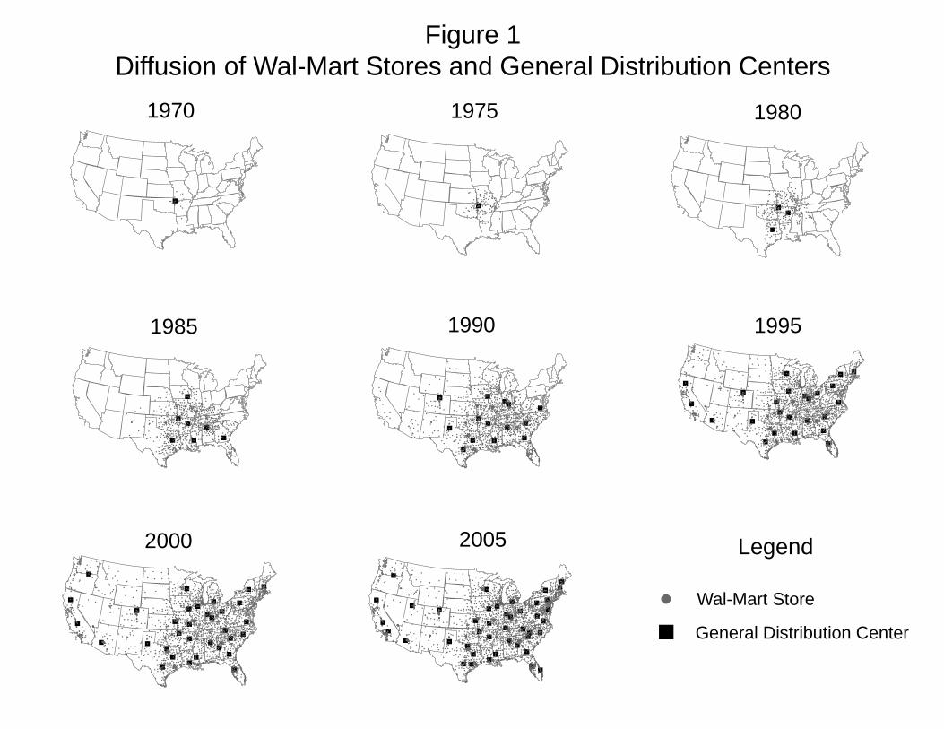
2005

""

"

"

"

""

""

"

""

""

"

"

"

"

"

" "

"

"

"

""

"

"

"

""

"

"

! !

!

!

!!

!

!

!

!!

!

!

!

!

!

!

!

!

!

!

!

!

!!

!

!

!

!

!

!

!

!

!

!

!

!

!

!

!!

!

!

!

!

!

!

!

!

!

!

!

!

!

!

!

!

!!

!!!

!

!

!

!

!

!

!

!

! !

!

!

!

!!

!

!

!

!

!

!

!

!

!

!

!

!

!

!!

!

!

!

!

!

!

!

!

!

!

!

!!

!

!

!

!

! !

!

!

!!

!!

!

!

!

!

!

!

!

!

!

!

!

!

!

!

!

!

!

!

!

!

!

!

!

!

!

!

! !

!

!

!

!

!!

!

!

!

!

! !

!

!

!

!

!

!

!

!

!

!

!

!

!

!!

!!

!

!

! !!

!

!

!!

!

!

!

!

!

!

!

!

!

!

!

!

!

!!

!

!

!

!

!

!

!

!

!

!

!

!

!

!

!

!!

!

!

!

!

!

!

!

!

!

!

!

!

!

!

!!

!!

!

!

!

!

!

!

!

!

!!!

!

!

!

!

!

!

!

!!

!

!

!

!

!

!

!

!

!

!!

!

!

!

!

!

!

!

!

!

!

!

!

!!

!

!

!

!

!

!

!

!!

!

!

!

!

!

!

!

!!

!

!

!

!

!!

!

!

!

!

!

!

!

!

!!

!

!

!

!

!

!

!

!

!

!

!!

!

!

! ! !

!

!

!

!!!

!

!

!

!

!!

!

!

!!

!

!

!

!

!

!

!!!

!

!

!!

!

!!

!

!

!

!

!

!!

!

!

!!

!

!

!

!!

!

!

!

!

!!

! !!

!

!

!

!

!

!

!

!

!

!

!

!

!

!

!

!

!

!

!

!

!!! !

!

!

!!

!

!!

!!

!

!

!

!

!

!

!

!

!

!

!

!

!

!

!

!

!

!

!

!

!

!

!

!

!

!

!

!!

!

!

!

!

!

!

!

!

!

!

!

! !

!

!

!

!

!

!

!

!

!

!

!!

!!

!

!

!

!

!

!!

!

!

!

!

!

! !

! !

!

!

!

!

!

!

!

!

!

!

!

!

!

!

!

!

! !!

!

!!

!

!

!

!

!

!

!

!

!

!

!

!

!

!

!

!

!

!

!

!

!

!

!

!

!

!

!

!

!

!

!

!

!

!

!

!

!!

!

!

!

!

!

!

!

!

!

!

!

!

!

!

!

!

!

!

!

!

!

!

!

!

!

!

!

!

!

!!

!

!

!

!

!

!

!

!

!!

!

!

!

!

!

!

!

!

!

!

!

!

!!

!

!

!

!

!

!

!

!

!

!!!

!!

!!

!

!

!

!

!

!

!

!

!

!

!

!

! !!

!

!

!

!

!!

!

!

!!

!!!

!!

!!

!

!

!!

!

!

!!

!

!

!

! !!

!

!

!

!

!

!

!

!

!!

!

!

!

!

!

!

!

!

!

!!

!

!

!

!

!

!

!

!

!

!

!

!

!

!

!

!

!

!

!

!

!

!

!

!

!

!

!

!

!

!!

!

!

!

!

!

!!

!

!

!

!

!

!!!

!

!

!

!

!

!

!!

!

!

!

!

!

!

!

!

!

!

!

!

!

!

!

!

!

!

!

!

!

!

!

!

!

!

!

!

!

!

!

!

!

! !

!

!

!

!

!

!

!

!

!

!

!

!

!

!

!

!

!

!

!

!

!

!

!

!

!

!

!

!

!

!

!

!

!

!

!

!

!

!

!

!

!

!

!

!

!

!!

!

!

!

!

!

!

!

!

!

!

!

!

!

!

!

!

!

!

!

!

!

!

!

!

!

!

!

!

!

!

!

!

!

!

!!

!

!

!

!

!

! !

!

!

!

!

!

!

!

!

!

!

!

!!

!

!

!

!!

!

!

!!

!

!

!

!

!

!

!

!

!

!

!!

!

!

!

!

!

!

!!

!

!

!

!

!

!

!

!

!

!

!

!

!

!

!

!!

!

!

!

!

!

!

!!

!!

!

!

!

!

!

!

!

!

!

!

!

!

!

!

!

!

!

!

!

!!

!

!

!

!!

!

!

!

!

!

!

!

!

!

!

!

!

!

!

!

!

!

!

!

!

!

!

!

!

!

!

!

!

!

!

!

!

!

!

!

!

!

!

!

!

!

!

!

!

!

!

!

!

!

!

!!

!

!

!

!

!

!

!

!

!

!

!

!

!

!

!

!

!

!

!

!

!

!

!

!

!

!

!

!

!

!!

!

!!

!

!

!

!

!

!

!

!

!

!

!

!

!

!

!

!

!!

!

!

!

!

!!

!

!

!

! !

!

!!

!

!

!

!!

!

!

!

!

!

!

!

! !

!

!

!

!

!

!

!!

!

!

!

!

!

!

!!

!

!

!

!

!

!

!

!

!

!

!

! !

!

!

!

!

!

!

!

!

!

!!

!

!

!

!

!

!

!

!

!

!

!

!!

!

!

!

!

!

!

!

!

!!

!

!

!

!

!

!

!

!

!

! !

!

!

!

!

!

!

!

!

!

!

!

!

!

!

!!

!!

!

!

!

!

!

!

!

!

!

!

!!

!

!

!

!

!

!

!

!

!

!

!

!

!

!

!

!

!

!

!

!

!

!

!

!

!

!

!

!

!

!

!!

!

!

!

!

!

!

!

!

!

!

!

!

!

!

!

!

!

!

!

!

!

!

!

!

!

!

!

!

!

!

!

!

!

!

!

!

!

!

!

!

!

!

!

!

!!!!

!!

!

!

!

!

!

!

!!

!

!

!

!

!

!

!

!

!

!

!

!

!

!

!

!

!

!

!!

!

!

!

!

!

!

! !

!

!

!

!

!

!!

!

!

!

!

!

!

!

!

!

!

!

!

!

!

!

!

!

!

!

!

!

!!

!

!

!

!

!

!

!

!

!

!

!

!

!

!

!

!

!

!

!

!

!

!

!

!

!

!

!

!

!

!

!

!

!

!

!

!

!

!

!

!

!

!

!

!

!

!

!

!

!

!

!

!

!

!

!

!

!

!

!

!

!

!

!

!

!

!

!

!

!

!

!

!

!

!

!

!!

!

!

!

!!

!

!

!

!

!!

!

!

!

!

!

!

!

!

!

!

!!

!

!

!

!

!

!

!

!

!

!

!

!

!!

!

!

!

!

!

!

!

!

!

!

!

!

!

!

!

!

!!

!!!

!

!

!

!

!

!

!!

!

!

!

!

!

!

!

!

!

!

!

!

!

!!

!

!

!

!

!

!

!

!

!

!!!

!

!

!

!

!

!

!

!

!

!

!

!

!

!

!!

!

!

!

!

!

!

!

!

!

!

!

!

!

!

!

!

!!

!

!

!

!

!

!

!

!

!

!

!

!

!

!

!

!

!

!!

!

!

!

!

!

!

!

!

!

!

!

!

!

!

!

!

!

!!

!

!

!

!

!

!

!

!

!

!

!

!

!

!!

!

!

!

!

!

!

!

!

!

!

!

! !!

!

!

!

!

!

!

!

!

!

!

!

!

!!

!

!

!

!

!

!

!

!

!

!!

!!

!

!!

!

!

!

!

!

!

! !

!

!!

!

!

! !

!

!

!

!! !

!!

!

!

!

!

!

!!

!

!

!

!

!

!

!

!

!

!

!

!

!

!

!

!

!

!

!

!

!

!

!

!

!

!

!

!

!

!

!

!

!

!

!

!

!

!

!

!

!

!

!

!

!

!

!

!

!

!

!

!

!

!

!

!

!

!

!

!

!!

!

!

!

!

!

!

!

!

!

!

!

!

!

!!

!

!

!

!

!

!

!

!

!

!

!

!

!

!

!

!

!

!

!

!

!

!

!

!

!

!

!!

!

!

!

!

!

!

!

!

!

!

!

!

!

!

!

!

!

!

!

!

!

!

!

!

!

!

!

!

!

!

!

!

!

!

!

!

!

!

!

!

!

!

!

!

!

!

!

!

!

!

!

!

!!

!!

!

!

!

!

!

!!

!

!!

!

!

!

!

!

!

! !

!!

!

!

!

!

!

!!

!

!

!

!

!

!

!

!

!

!

!

!

!

!

!

!

!

!

!

!

!

!

!

!

!

!

!

!

!

!

!

!

!

!

!

!

!

!

!

!

!

!

!

!

!

!

!

!

!

!!

!

!

!

!

!

!

!

!

!

!!!

!

!

!

!

!

!

!

!

!

!

!

!

!

!

!

!

!

!

!

!

!

!!

!

!

!

!

!

!

!

!

!

!

!

!!

!

!

!

!

!

!

!

!

!!

!

!

!

!

!

!

!

!

!

!

!

!

!

!

!

!

!

!!

!

!

! !

!

!

!

!

!

!

!

!

!

!

!

!

!

!

!

!

!

!

!

!

!

!

!

!

!

!

!

!

!

!

!

!

!

!

!

!

!

!!

!

!

!

!

!!

!

!

!!

!

!

!

!

!

!

!

!

!

!

!!

!

!

!

!

!

!!

!

!

!

!

!

!

!

!

!

!

!

!

!

!

!

!

!

!

!

!

!

!

!

!

!

!

!

!!

!

!

!

!

!

!

!

!

!

!

!

!

!

!

!

!

!

!

!

!

!

!

!

!

!

!

!

!

!

!

!

!

!

!

!

!

!

!

!

!

!

!

!

!

!!!

!

!

!

!

!

!

!

!

!

!

!

!

!

!

!

!

!

!

!

!

!

!

!

!

!

!

!

!

!!

!

!

!

!

!

!

!

!

!

!

!

!

!

!

!

!

!

!

! !

!

!

!

!

!

!

!

!

!

!

!

!

!

!

!

!

!

!

!

!

!

!

!

!

!

!

!

!

!

!

!

!

!

!

!

!

!

!

!

!

!

!

!

!

!

!

!

!

!

!

!

!

!

!

!

!

!

!

!

!

!

!

!

!

!

!

!

!

!

!

!

!

!

!

!

!

!

!

!

!

!

!

!

!!

!!

!

!

!

!!

!

!

!

!

!

!

!

!

!

!

!

!

!

!

!

!

!

!

!

!

!

!

!

!

!

!

!

!!

!

!

!

!

!

!

!

!

!

!

!

!

!

!

!

!

!

!

!

!

!

!

!

!

!

!

!

!

!

!

!

!

!

!!

!

!

!

!

!

!

!!

!

!

!

! !

!!

!

!

!

!

!

!

!

!

!

!

!

!

!

!

!

!

!

!

!

!!

!

!

!

!

!

!!

!

!

!

!

!

!

!

!

!

!

!

!

!

!

!

!

!

!

!

!

!

!

!

!

!

!

!

!

!

!

!

!

!

!

!

!

!!

!

!!

!

!

!

!

!

!

!

!

!

!

!

!

!

!

!

!

!

!

!

!!!!

!!

!

!

!

!

!

!

!

!

!

!

!

!

!

!

!

!

!

!

!

!

!

!

!

!

!!

!

!

!

!

!

!

!

!

!

!!

!

!

!

!

!!

!

!!

!

!

!

!

!!

!

!

! !!

!

!

!

!

!

!

!

!!

!

!

!

!

!!

!

!

!

!

!!

!!

!

!

!

!

!

!

!

!

!

!

!

!!

!

!

!

!

!

!

!

!

! !

!

!

!

!

!!

!

!

!

!

!

!

!

!

!!!!

!

!

!

! !

!

!

!

!

!

!

!

!

!

!

!

!

!

!

!

!

!

!

!

!

!

!

!

!

!

!

!

2000

""

"

"

"

""

""

"

""

""

"

"

"

"

"

" "

"

"

"

! !

!

!

!!

!

!

!

!!

!

!

!

!

!

!

!

!

!

!

!

!

!!

!

!

!

!

!

!

!

!

!

!

!

!

!

!

!!

!

!

!

!

!

!

!

!

!

!

!

!

!

!

!

!

!!

!!!

!

!

!

!

!

!

!

!

! !

!

!

!

!!

!

!

!

!

!!

!

!

!

!

!

!

!

!!

!

!

!

!

!

!

!

!

!

!

!

!!

!

!

!

!

! !

!

!

!!

!!

!

!

!

!

!

!!

!

!

!

!

!

!

!

!

!

!

!

!

!

!

!

!

!

!

!

! !

!

!

!

!

!!

!

!

!

!

! !

!

!

!

!

!

!

!

!

!

!

!

!

!

!!

!!

!

!

! ! !

!

!

!!

!

!

!

!

!

!

!

!

!

!

!

!

!

!!

!

!

!

!

!

!

!

!

!

!

!

!

!

!

!

!!

!

!

!

!

!

!

!

!

!

!

!

!

!

!

!!

!!

!

!

!

!

!

!

!

!

!!!

!

!

!

!

!

!

!

!!

!

!

!

!

!

!

!

!

!

!!

!

!

!

!

!

!

!

!

!

!

!

!

!!

!

!

!

!

!

!

!

!!

!

!

!

!

!

!

!

!!

!

!

!

!

!!

!

!

!

!

!

!

!

!

!!

!

!

!

!

!

!

!

!

!

!

!!

!

!

! ! !

!

!

!

!!!

!

!

!

!

!!

!

!

!!

!

!

!

!

!

!

!!!

!

!

!!

!

!!

!

!

!

!

!

!!

!

!

!!

!

!

!

!!

!

!

!

!

!!

! !!

!

!

!

!

!

!

!

!

!

!

!

!

!

!

!

!

!

!

!

!

!!! !

!

!

!!

!

!!

!!

!

!

!

!

!

!

!

!

!

!

!

!

!

!

!

!

!

!

!

!

!

!

!

!

!

!

!

!!

!

!

!

!

!

!

!

!

!

!

!

! !

!

!

!

!

!

!

!

!

!

!

!!

!!

!

!

!

!

!

!!

!

!

!!

!

! !

! !

!

!

!

!

!

!

!

!

!

!

!

!

!

!

!

!

! !!!

!!

!

!

!

!

!

!

!

!

!

!

!

!

!

!

!

!

!

!

!

!

!!

!

!

!

!

!

!

!

!

!

!

!

!

!

!

!!

!

!

!

!

!

!

!

!

!

!

!

!

!

!

!

!

!

!

!

!

!

!

!

!

!

!

!

!

!

!!

!

!

!

!

!

!

!

!

!!

!

!

!

!

!

!

!

!

!

!

!

!

!!

!

!

!

!

!

!

!

!

!

!!!

!!

! !

!

!

!

!

!

!

!

!

!

!

!

!

! !!

!

!

!

!

!!

!

!

!!

! !!!

!!!

!

!

!!

!

!

!!

!

!

!

! !!

!

!

!

!

!

!

!

!

!!

!

!

!

!

!

!

!

!

!

!!

!

!!

!

!

!

!

!

!

!

!

!

!

!

!

!

!

!

!

!

!

!

!

!

!

!

!

!

!

!!

!

!

!

!

!

!!

!

!

!

!

!

!!!

!

!

!

!

!

!

!!

!

!!

!

!

!

!

!

!

!

!

!

!

!

!

!

!

!

!

!

!

!

!

!

!

!

!

!

!

!

!

!

!

! !

!

!

!

!

!

!

!

!

!

!

!

!

!

!

!

!

!

!

!

!

!

!

!

!

!

!

!

!

!

!

!

!

!

!

!

!

!

!

!

!

!

!

!

!

!

!!

!

!

!

!

!

!

!

!

!

!

!

!

!

!

!

!

!

!

!

!

!

!

!

!

!

!

!

!

!

!

!

!

!

!

!!

!

!

!

!

!

! !

!

!

!

!

!

!

!

!

!

!

!

!!

!

!

!

!!

!

!

!!

!!

!

!

!

!

!

!

!

!

!!

!

!

!

!

!

!

!!

!

!

!

!

!

!

!

!

!

!

!

!!

!

!

!!

!

!

!

!

!

!

!!

!!

!

!

!

!

!

!

!

!

!

!

!

!

!

!

!

!

!

!

!

!!

!

!

!

!!

!

!

!

!

!

!

!

!

!

!

!

!

!

!

!

!

!

!

!

!

!

!

!

!

!

!

!

!

!

!

!

!

!

!

!!!

!

!

!

!

!

!

!

!

!

!

!

!

!

!!

!

!

!

!

!

!

!

!

!

!

!

!

!

!

!

!

!

!

!

!

!

!

!

!

!

!

!

!

!

!!

!! !

!

!

!

!

!

!

!

!

!

!

!

!

!

!

!

!

!!

!

!

!

!

!!

!

!

!

! !

!

!!

!

!

!

!!

!

!

!

!

!

!

!

! !!

!

!

!

!

!

!!

!

!

!

!

!

!

!!

!

!

!

!

!

!

!

!

!

!

!

! !

!

!

!

!

!

!

!

!

!

!!

!

!

!

!

!

!

!

!

!

!

!

!!

!

!

!

!

!

!

!

!

!!

!

!

!

!

!

!

!

!

!

! !

!

!

!

!

!

!

!

!

!

!

!

!

!

!

!!

!!

!

!

!

!

!

!

!

!

!

!

!!!

!

!

!

!

!

!

!

!

!

!

!

!

!

!

!

!

!

!

!

!

!

!

!

!

!

!

!

!

!

!!

!

!

!

!!

!

!

!

!

!

!

!

!

!

!!

!

!

!

!

!

!

!

!

!

!

!

!

!

!

!

!

!

!

!

!

!

!

!

!

!

!

!

!

!!!!

!!

!

!

!

!

!

!

!!

!

!

!

!

!

!

!

!

!

!

!

!

!

!

!

!

!

!

!!

!

!

!

!

!

!

! !

!

!

!

!

!

!!

!

!

!

!

!

!

!

!

!

!

!

!

!

!

!

!

!

!

!

!

!

!!

!

!

!

!

!

!

!

!

!

!

!

!

!

!

!

!

!

!

!

!

!

!

!

!

!

!

!

!

!

!

!

!

!

!

!

!

!

!

!

!

!

!

!

!

!

!

!

!

!

!

!

!

!

!

!

!

!

!

!

!

!

!

!

!

!

!

!

!

!

!

!

!

!

!

!

!!

!

!

!

!!

!

!

!

!

!!

!

!

!

!

!

!

!

!

!

!

!!

!

!

!

!

!

!

!

!

!

!

!

!

!!

!

!

!

!

!

!

!

!

!

!

!

!

!

!

!

!

! !

!!!

!

!

!

!

!

!

!!

!

!

!

!

!

!

!

!

!

!

!

!

!

!!

!

!

!

!

!

!

!

!

!

!!!

!

!

!

!

!

!

!

!

!

!

!

!

!

!

!!

!

!

!

!

!

!

!

!

!

!

!

!

!

!

!

!

!!

!

!

!

!

!

!

!

!

!

!

!

!

!

!

!

!

!

!!

!

!

!

!

!

!

!

!

!

!

!

!

!

!

!

!

!

!!

!

!

!

!

!

!

!

!

!

!

!

!

!

!!

!

!

!

!

!

!

!

!

!

!

!

! !!

!

!

!

!

!

!

!

!

!

!

!

!

!!

!

!

!

!

!

!

!

!

!

! !

!!

!

!!

!

!

!

!

!

!

! !

!

!!

!

!

! !

!

!

!

!! !

!!

!

!

!

!

!

!!

!

!

!

!!

!

!

!

!

!

!

!

!

!

!

!

!

!

!

!

!

!

!

!

!

!

!

!

!

!

!

!

!

!

!

!

!

!

!

!

!

!

!

!

!

!

!

!

!

!

!

!

!

!

!

!

!

!

!

!

!!

!

!

!

!

!

!

!

!

!

!

!

!!

!!

!

!

!

!

!

!

!

!

!

!

!

!

!

!

!

!

!

!

!

!

!

!

!

!

!

!

!!

!

!

!

!

!

!

!

!

!

!

!

!

!

!

!

!

!

!

!

!

!

!

!

!

!

!

!

!

!

!

!

!

!

!

!

!

!

!

!

!

!

!

!

!

!

!

!

!

!

!

!!

!

!!

!

!

!

!

!

!!

!

!!

!

!

!

!

!

!

! !

!!

!

!

!

!

!

! !

!

!

!

!

!

!

!

!

!

!

!

!

!

!

!

!

!

!

!

!

!

!

!

!

!

!

!

!

!

!

!

!

!

!

!

!

!

!

!

!

!

!

!

!

!

!

!

!

!

!!

!

!

!

!

!

!

!

!

!

!!!

!

!

!

!

!

!

!

!

!

!

!

!

!

!

!

!

!

!

!

!

!

!!

!

!

!

!

!

!

!

!

!

!

!

!!

!!

!

!

!

!

!

!

!!

!

!

!

!

!

!

!

!

!

!

!

!

!

!

!

!

!

!!

!

!

! !

!

!

!

!

!

!

!

!

!

!

!

!

!

!

!

!

!

!

!

!

!

!

!

!

!

!

!

!

!

!!

!

!

!

!

!!

!

!

!

!

!!

!

!

!!

!

!

!

!

!

!

!

!

!

!

!!

!

!

!

!

!!

!

!

!

!

!

!

!

!

!

!

!

!

!

!

!

!

!

!

!

!

!

!

!

!

!

!

!

!

!

!

!

!

!

!

!

!

!

!

!!

!

!

!

!

!

!

!

!

!

!

!

!

!

!

!

!

!

!

!

!

!

!

!

!!!

!

!

!

!

!

!

!

!

!

!

!

!

!

!

!

!

!

!

!

!

!

!

!

!

!

!

!

!

!

!

!

!

!

!

!

!

!

!

!

!

!

!

!

!

!

!

!

!

!

!

!

!

!

!

!

!

!

!

!

!

!

!

!

!

!

!

!

!

!

!

!

!

!

!

!

!

!

!

!

!

!

!

!

!

!

!!

1995

""

"

"

"

""

""

"

""

""

! !

!

!

!!

!

!

!

!!

!

!

!

!

!

!

!

!

!

!

!

!

!!

!

!

!

!

!

!

!

!

!

!

!

!

!

!

!!

!

!

!

!

!

!

!

!

!

!

!

!

!

!

!

!

!!

!!!

!

!

!

!

!

!

!

!

! !

!

!

!

!!

!

!

!

!

!!

!

!

!

!

!

!

!

!!

!

!

!

!

!

!

!

!

!

!

!

!!

!

!

!

!

! !

!

!

!!

!!

!

!

!

!

!

!!

!

!

!

!

!

!

!

!

!

!

!

!

!

!

!

!

!

!

!

! !

!

!

!

!

!!

!

!

!

!

! !

!

!

!

!

!

!

!

!

!

!

!

!

!

!!

!!

!

!

! ! !

!

!!

!

!

!

!

!

!

!

!

!

!

!

!

!

!!

!

!

!

!

!

!

!

!

!

!

!

!

!

!

!

!!

!

!

!

!

!

!

!

!

!

!

!

!

!

!

!!

!!

!

!

!

!

!

!

!

!

!!!

!

!

!

!

!

!

!

!!

!

!

!

!

!

!

!

!

!

!!

!

!

!

!

!

!

!

!

!

!

!

!

!!

!

!

!

!

!

!

!

!!

!

!

!

!

!

!

!

!!

!

!

!

!

!!

!

!

!

!

!

!

!

!

!!

!

!

!

!

!

!

!

!

!

!

!!

!

!

! ! !

!

!

!

!!!

!

!

!

!

!!

!

!

!!

!

!

!

!

!

!

!!!

!

!

!!

!

!!

!

!

!

!

!

!!

!

!

!!

!

!

!

!!

!

!

!

!

!!

! !!

!

!

!

!

!

!

!

!

!

!

!

!

!

!

!

!

!

!

!

!

!!! !

!

!

!!

!

!!

!!

!

!

!

!

!

!

!

!

!

!

!

!

!

!

!

!

!

!

!

!

!

!

!

!

!

!

!

!!

!

!

!

!

!

!

!

!

!

!

!

! !

!

!

!

!

!

!

!

!

!

!

!!

!!

!

!

!

!

!

!!

!

!

!!

!

! !

! !

!

!

!

!

!

!

!

!

!

!

!

!

!

!

!

!

! !!!

!!

!

!

!

!

!

!

!

!

!

!

!

!

!

!

!

!

!

!

!

!

!!

!

!

!

!

!

!

!

!

!

!

!

!

!

!

!!

!

!

!

!

!

!

!

!

!

!

!

!

!

!

!

!

!

!

!

!

!

!

!

!

!

!

!

!

!

!!

!

!

!

!

!

!

!

!

!!

!

!

!

!

!

!

!

!

!

!

!

!

!!

!

!

!

!

!

!

!

!

!

!!!

!!

!!

!

!

!

!

!

!

!

!

!

!

!

!

! !!

!

!

!

!

!!

!

!

!!

!!!

!!

!!

!

!

!!

!

!

!!

!

!

!

! !!

!

!

!

!

!

!

!

!

!!

!

!

!

!

!

!

!

!

!

!!

!

!!

!

!

!

!

!

!

!

!

!

!

!

!

!

!

!

!

!

!

!

!

!

!

!

!

!

!

!!

!

!

!

!

!

!!

!

!

!

!

!

!!!

!

!

!

!

!

!

!!

!

!!

!

!

!

!

!

!

!

!

!

!

!

!

!

!

!

!

!

!

!

!

!

!

!

!

!

!

!

!

!

!

! !

!

!

!

!

!

!

!

!

!

!

!

!

!

!

!

!

!

!

!

!

!

!

!

!

!

!

!

!

!

!

!

!

!

!

!

!

!

!

!

!

!

!

!

!

!

!!

!

!

!

!

!

!

!

!

!

!

!

!

!

!

!

!

!

!

!

!

!

!

!

!

!

!

!

!

!

!

!

!

!

!

!!

!

!

!

!

!

! !

!

!

!

!

!

!

!

!

!

!

!

!!

!

!

!

!!

!

!

!!

!

!

!

!

!

!

!

!

!

!

!!

!

!

!

!

!

!

!!

!

!

!

!

!

!

!

!

!

!

!

!!

!

!

!!

!

!

!

!

!

!

!!

!!

!

!

!

!

!

!

!

!

!

!

!

!

!

!

!

!

!

!

!

!!

!

!

!

!!

!

!

!

!

!

!

!

!

!

!

!

!

!

!

!

!

!

!

!

!

!

!

!

!

!

!

!

!

!

!

!

!

!

!

!

!

!

!

!

!

!

!

!

!

!

!

!

!

!

!

!!

!

!

!

!

!

!

!

!

!

!

!

!

!

!

!

!

!

!

!

!

!

!

!

!

!

!

!

!

!

!!

!

!!

!

!

!

!

!

!

!

!

!

!

!

!

!

!

!

!

!!

!

!

!

!

!!

!

!

!

! !

!

!!

!

!

!

!!

!

!

!

!

!

!

!

! !

!

!

!

!

!

!

!!

!

!

!

!

!

!

!!

!

!

!

!

!

!

!

!

!

!

!

! !

!

!

!

!

!

!

!

!

!

!!

!

!

!

!

!

!

!

!

!

!

!

!!

!

!

!

!

!

!

!

!

!!

!

!

!

!

!

!

!

!

!

! !

!

!

!

!

!

!

!

!

!

!

!

!

!

!

!!

!!

!

!

!

!

!

!

!

!

!

!

!!

!

!

!

!

!

!

!

!

!

!

!

!

!

!

!

!

!

!

!

!

!

!

!

!

!

!

!

!

!

!

!!

!

!

!

!!

!

!

!

!

!

!

!

!

!

!!

!

!

!

!

!

!

!

!

!

!

!

!

!

!

!

!

!

!

!

!

!

!

!

!

!

!

!

!

!!!!

!!

!

!

!

!

!

!!

!

!

!

!

!

!

!

!

!

!

!

!

!

!

!

!

!

!

!

!

!

!

!

!

!

! !

!

!

!

!

!

!!

!

!

!

!

!

!

!

!

!

!

!

!

!

!

!

!

!

!

!

!

!!

!

!

!

!

!

!

!

!

!

!

!

!

!

!

!

!

!

!

!

!

!

!

!

!

!

!

!

!

!

!

!

!

!

!

!

!

!

!

!

!

!

!

!

!

!

!

!

!

!

!

!

!

!

!

!

!

!

!

!

!

!

!

!

!

!

!

!

!

!

!

!

!

!!

!

!

!

!!

!

!

!

!

!

!

!

!

!

!

!

!

!

!!

!

!

!

!

!

!

!

!

!

!

!!

!

!

!

!

!

!

!

!

!

!

!

!

!

!

!

!

!!

!!

!

!

!

!

!

!!

!

!

!

!

!

!

!

!

!

!

!

!

!!

!

!

!

!

!

!

!

!!!

!

!

!

!

!

!

!

!

!

!

!

!

!!

!

!

!

!

!

!

!

!

!

!

!

!

!

!!

!

!

!

!

!

!

!

!

!

!

!

!

!

!

!

!

!

!

!

!

!

!

!!

!

""

"

"

"

""

! !!

!!

!

!

!

!!

!

!

!

!

!

!

!

!

!

!

!

!!

!

!

!

!

!

!

!

!

!

!

!

!

!

!

!!

!

!

!

!

!

!

!

!

!

!

!

!

!

!

!

!

!!

!!!

!

!

!

!

!

!

!

!

! !

!

!

!

!!

!

!

!

!

!!

!

!

!

!

!

!

!

!!

!

!

!

!

!

!

!

!

!

!

!

!!

!

!

!

!

! !

!

!

!!

!!

!

!

!

!

!

!!

!

!

!

!

!

!

!

!

!

!

!

!

!

!

!

!

!

!

!

! !

!

!

!

!

!!

!

!

!

!

! !

!

!

!

!

!

!

!

!

!

!

!

!

!

!!

!!

!

!

! ! !

!

!!

!

!

!

!

!

!

!

!

!

!

!

!

!

!!

!

!

!

!

!

!

!

!

!

!

!

!

!

!

!

!!

!

!

!

!

!

!

!

!

!

!

!

!

!

!

!!

!!

!

!

!

!

!

!

!

!

!!

!

!

!

!

!

!

!

!!

!

!

!

!

!

!

!

!

!

!!

!

!

!

!

!

!

!

!

!

!

!

!

!!

!

!

!

!

!

!

!

!!

!

!

!

!

!

!

!

!!

!

!

!

!

!!

!

!

!

!

!

!

!

!

!!

!

!

!

!

!

!

!

!

!

!

!!

!

!

! ! !

!

!

!

!!!

!

!

!

!

!!

!

!

!!

!

!

!

!

!

!

!!!

!

!

!!

!

!!

!

!

!

!

!

!!

!

!

!!

!

!

!

!!

!

!

!

!

!!

! !!

!

!

!

!

!

!

!

!

!

!

!

!

!

!

!

!

!

!

!

!

!!! !

!

!

!!

!

!!

!!

!

!

!

!

!

!

!

!

!

!

!

!

!

!

!

!

!

!

!

!

!

!

!

!

!

!

!

!!

!

!

!

!

!

!

!

!

!

!

! !

!

!

!

!

!

!

!

!

!

!

!!

!!

!

!

!

!

!

!!

!

!

!!

!

! !

! !

!

!

!

!

!

!

!

!

!

!

!

!

!

!

!

!

! !!!

!!

!

!

!

!

!

!

!

!

!

!

!

!

!

!

!

!

!

!

!

!

!!

!

!

!

!

!

!

!

!

!

!

!

!

!

!

!!

!

!

!

!

!

!

!

!

!

!

!

!

!

!

!

!

!

!

!

!

!

!

!

!

!

!

!

!

!!

!

!

!

!

!

!

!

!

!!

!

!

!

!

!

!

!

!

!

!

!

!

!!

!

!

!

!

!

!

!

!

!

!!!

!!

!!

!

!

!

!

!

!

!

!

!

!

!

! !!

!

!

!

!

!!

!

!

!!

!!!

!!!

!

!

!!

!

!

!!

!

!

!

! !!

!

!

!

!

!

!

!

!

!!

!

!

!

!

!

!

!

!

!

!!

!

!!

!

!

!

!

!

!

!

!

!

!

!

!

!

!

!

!

!

!

!

!

!

!

!

!

!

!

!!

!

!

!

!

!

!!

!

!

!

!

!

!!!

!

!

!

!

!

!

!!

!

!!

!

!

!

!

!

!

!

!

!

!

!

!

!

!

!

!

!

!

!

!

!

!

!

!

!

!

!

!

!

! !

!

!

!

!

!

!

!

!

!

!

!

!

!

!

!

!

!

!

!

!

!

!

!

!

!

!

!

!

!

!

!

!

!

!

!

!

!

!

!

!

!

!!

!

!

!

!

!

!

!

!

!

!

!

!

!

!

!

!

!

""

"

! !!

!!

!

!

!

!!

!

!

!

!

!

!

!

!

!

!

!

!!

!

!

!

!

!

!

!

!

!

!

!

!

!

!

!!

!

!

!

!

!

!

!

!

!

!

!

!

!

!

!

!

!!

!!!

!

!

!

!

!

!

!

!

! !

!

!

!!

!

!

!

!

!!

!

!

!

!

!

!

!

!!

!

!

!

!

!

!

!

!

!

!

!

!!

!

!

!

!

! !

!

!

!!

!!

!

!

!

!

!

!!

!

!

!

!

!

!

!

!

!

!

!

!

!

!

!

!

!

!

!

! !

!

!

!

!

!!

!

!

!

!

! !

!

!

!

!

!

!

!

!

!

!

!

!

!!

!!

!

!

! ! !

!

!!

!

!

!

!

!

!

!

!

!

!

!

!!

!

!

!

!

!

!

!

!

!

!

!

!

!

!

!

!!

!

!

!

!

!

!

!

!

!

!

!

!

!

!

!!

!!

!

!

!

!

!

!

!

!

!!

!

!

!

!

!

!

!!

!

!

!

!

!

!

!

!

!

!

!

!

!

!

!

!

!

!

!

!

!!

!

!

!

!

!

!

!!

!

!

!

!

!

!!

!

!

!

!!!

!

!

!

!

!!

!

!

!

!

!

!

!!

!

! !

!

!!

!

!

!!!

"! !!

!!

!

!

!

!!

!

!

!

!

!

!

!

!

!

!

!

!!

!

!

!

!

!

!

!

!

!

!

!

!

!

!

!!

!

!

!

!

!

!

!

!

!

!

!

!

!

!

!

!

!!

!!!

!

!

!

!

!

!

!

!

! !

!

!!

!

!

!

!

!!

!

!

!

!

!

!

!

!!

!

!

!

!

!

!

!

!

!

!!

!

!

!

!

! !

!

!

!

!

!

!

!

!

!

!

"! !!

!!

!

!

!!

!

!

!

!

!

!

!

!

!

!

!

19901985

198019751970

Diffusion of Wal-Mart Stores and General Distribution CentersFigure 1

Legend

! Wal-Mart Store

" General Distribution Center

"

"

"

"

""

"

"

"

"

"

"

"

"

"

"

"

"

"

"

""

"

""

"

"

"

" "

"

"

"

"

"

! !

!

!

!!

!

!

!!

!

!

!

!

! !

!

!

!

!

!

!

!

!

!

!

!

!

!

!

!

!

!

!

!

!

!

!

!

!

!

!

!

!

!

!

!

!

!!

!!

!

!

!

!

!

!

!

!

!

!

!

!

!

!

!

!

!

!

!

!

!

!

!

!

!

!

!

!

!

!

!

!!

!

!

!

!

!

!

!!

!

!

!

!

!

!

!

!

!

!

!

!

!

!

!

!

! !

!

!

!

!

!!

!

!

!

! !

!

!

!

!

!

!

!

!

!

!

!

!!

!

!

! !!

!

!

!

!

!

!

!

!

!

!

!

!

!!

!

!

!

!

!

!

!

!

!

!!

!

!

!

!

!

!

!

!

!

!!

!

!

!

!

!

!

!

!

!!

!

!

!

!

!

!

!

!!

!

!

!

!

!

!

!

!

!

!

!

!

!

!

!

!

!

!

!

!

!

!

!

!

!!

!

!

!

!

!

!

!!

!

!

!!

!

!

!

!

!

!

!

!

!

!

!

!

!

!!

! !

!

!

!!

!

! !!

!

!

!

!

!

!

!

!

!

!

!

!! !

!

!

!

!

!

!

!

!!

!

!

!

!

!

!

!

!

!

!

!

!

!

!

!

!! !

!

!

!!

!

!!

!

!

!

!

!

!

!

!

!

!

!

!

!

!

!

!

!!

!

!

!

!

!

!

!

!

!

!

!

!

!

!

!

!

!!

!

!

!

!

!!

!

!

! !

! !

!

!

!

!

!!

!

!

!

!

!

!

!

! !!

!

!!

!

!

!

!

!

!

!

!

!

!

!!

!

!

!

!

!

!

!

!

!

!

!

!

!

!

!!

!

!

!

!

!

!

!

!

!

!

!

!

!

!

!

!

!

!

!

!

!

!

!

!

!

!

!

!

!

!

!

!

!

!

!!!

!

!

!

!

!

!

!

!

!

!

!

!

!

!

!!

!!

!

!

!

!

!

!

!

!

!

!

! !!

!

!

!

!

!

!

!

!

!!

!!

!!

!

!!

!

!

!!

!

!

!

!

!

!

!

!

!

!

!

!

!

!!

!

!

!

!

!

!

!

!

!

!

!

!

!

!

!

!

!

!

!

!

!

!

!

!

!

!

!

!

!

!

!

!

!

!

!

!

!

!

!

!!

!

!

!

!!

!

!

!

!

!

!

!!

! !

!

!

!

!

!

!

!

!

!

!

!

!

!

!

!

!

!

!

!

!! !

!

!

!

!

!

!

!

!

!

!

!

!

!

!

!

!

!

!

!

!

!

!

!

!

!

!

!

!

!

!

!

!

!

!

!!

!

!

!

!

!

!

!

!

!

!

!

!

!

!

!

!

!

!

!

!

!

!

!

!

!

!

!

! !

!

!!

!

!

!

!

!

!

!

!

!

!

!

!

!

!

!

!

!!

!

!

!

!

!

!

!

!!

!

!

!

!

!!

!

! !

!

!

!

!

!

!!!

!

!

!

!

!

!

!

!!

!

!

!

!

!

!

!

!

!

!

!

!

!!

!

!

!

!

!

!

!

!

!

!

!

!

!

!

!

!

!

!

!

!

!

!

!

!

!

!

!

!

!

!

!

!

!

!

!

!

!

!

!!

!

!

!

!

!

!

!

!

!

!

!

!

!

!

!

!

!

!

!

!

!!

!

!

!

!

!

!

!

!

!!

!!

!

!

!

!

!

!

!!

!

!

!

!

!

! !

!

!

!

!

!

!

!

!

!

!

!

!

!

!

!

!

!

!

!

!

!!

!

!

!

!

!

!

!

!

!

!

!

!

!

!

!

!

!

!

!

!! !

!

!

!

!

!

!

!

!

!

!!

!

!

!

!

!

!

!

!

!!

!

!

!

!

!

!

!

!

!

!

!

!

!

!

!

!

!

!

!

!

!

!

!

!

!

!

!

!

!

!

!

!

!

!

!

!

!

!

!

!

!

!

!

!

!

!

!

!

!!!

!!

!

!

!

!

!

!

!

!

!

!

!

!

!

!

!

!!

!

!

!

!

!

! !

!

!

!

!

!

!

!

!

!

!

!

!

!

!

!

!

!

!

!

!

!

!

!

!

!

!

!

!

!

!

!

!

!

!

!

!

!

!

!

!

!

!

!

!

!

!

!

!

!

!

!

!

!

!

!

!

!

!

!

!

!

!

!

!

!

!

!

!

!

!

!

!

!

!

!

!

!

!

!

!

!!

!

!

!

!

!

!

!

!

!

!

!

!

!

!

!

!

!

!

!

!!

!!!

!

!

!

!

!

!

!

!

!

!

!

!

!

!

!

!

!

!

!

!

!

!

!

!

!

!

!

!

!

!

!

!

!

!

!

!

!

!

!

!

!

!

!

!!

!

!

!

!

!

!

!

!

!!

!

!

!

!

! !!!

!

!

!

!

!

!

!

!

!

!

!!

!

!

!

!

! !

!

!

!

!

!

!!

!!

!

!

!

!

!

!

!

!

!

!

!

!

!

!

!

!

!

!

!

!

!

!

!

!

!

!

!

!

!

!

!

!

!

!

!!

!

!

!

!

!

!

!

!

!

!

!!

!

!

!

!

!

!

!

!

!

!

!

!

!

!

!

!

!

!

!

!

!

!

!!

!

!

!

!

!

!

!

!

!

!

!

!

!

!

!

!

!

!

!

!

!

!

!

!

!

!

!

!

!

!

!

!

!

!

!

!

!

!

!

!

!

!

!

!

!

!

!

!

!

!

!!

!

!

!

!

!

!

!

!

!

!

!

!

!

!

!

!

!

!

!

!

!

!

!

!

!

!

!

!

!

!

!

!

!

!

!

!

!

!

!

!

!

!

!

!

!

!

!

!

!

!

!

!

!

!

!

!

!

!

!

!

!

!

!

!

!

!

!!

!

!

!

!

!

!

!

!

!

!

!

!

!

!

!

!

!

!

!

!

!

!

!

!

!

!

!

!

! !!

!

!

!

!

!

!

!

!

!

!

!

!

!

!

!

!

!

!

!

!

!

!

!

!

!

!

!

!

!

!

!

!

!

!

!

!

!

!

!

!

!

!

!

!

!

!!

!

!

!

!

!

!

!

!

!

!

!

!

!

!

!

!

!

!

!!

!

!

!

!

!

!

!

!

!

!

!

!

!

!

!

!

!

!

!!

!

!

!

!

!

!

!

!

!

!

!

!

!

!

!

!!!!

!

!

!

!

!

!

!

!

!

!

!

!

!

!

!

!

!

!

!

!

!

!!

!

!

!

!

!

!

!

!

!

!

!

!

!

!

!

!

!

!!

!

!!!

!

!

!

!

!!

!

!

!!!!

!

!

!

!

!

!

!

!!

!

!

!

!

!!

!

!

!

!

!

!

!

!

!

!

!

!

!

!

!!

!

!

!

!

!

!

!

!

! !!

!

!

!!

!

!

!

!

!

!

!!

!

!

!

!

!

!

!

!

!

!

!

!

!

!

!

!

!

!

!

!

!

!

!

!

!

!

!

!

!

!

!

!

!

!!

!

!

!

!!

!

!

!

!

!

!

!

!

!!

!

!

!

!

!

!

! !

!

!

!

!

!

!

!!

!

!

!

!

!

!

!

!

!

!

!

!

!

!

!

!

!

!

!

!

!

!

!

!

!

!

!

!

!

!

!

!

!

!

!

!

!

!

!

!

!

!

!

!

!!

!

!

!

!!

!

!

!

!

!

!

!

!

!

!

!

!

!

!

!

!!

!

!!

!

!

!

!

!

!

!

!

!

!

!!

!

!

!

! !

!

!

!

!

!

!

!

!

!

!

!

!

!

!

!

!

!

!

!

!

!

!

!

!

!

!!

!

!

!

!

!

!

!

!

!!

!

!

!

!

!

!

!

!!

!

!

!

!

!

!

!

!

!

!

!

!

!

!

!

!

!

!!

!

!

!

!

!

!

!

!

!

!

!!

!

!

!

!

!

!

!

!

!

!

!

!

!

!

!

!

!

!

!

!

! !

!

!

!

! !

!!!

!

!

!

!

!

!

!

!

!

!

!

!

!

!

!

!!

!!!

!

! !

!

!

!!

!

!!

!

!

!

!

!

!

!

!

!

!

!

!

!

!

!!

!

!

!

!

!

!

!

!

!

!

!

!

!

!

!

!

!

!

!

!

!

!

!

!!!

!!

!

!

!

!

!! !

!

!

!

!

!

!

!

!

!

!

!

!

!

!

!

!

!

!

!

! !

!

!

!

!!

!

!

!

!

!

!

!

!

!

!

!

!

!

!

!

!

!

!

!

!!

!

!

!

!!

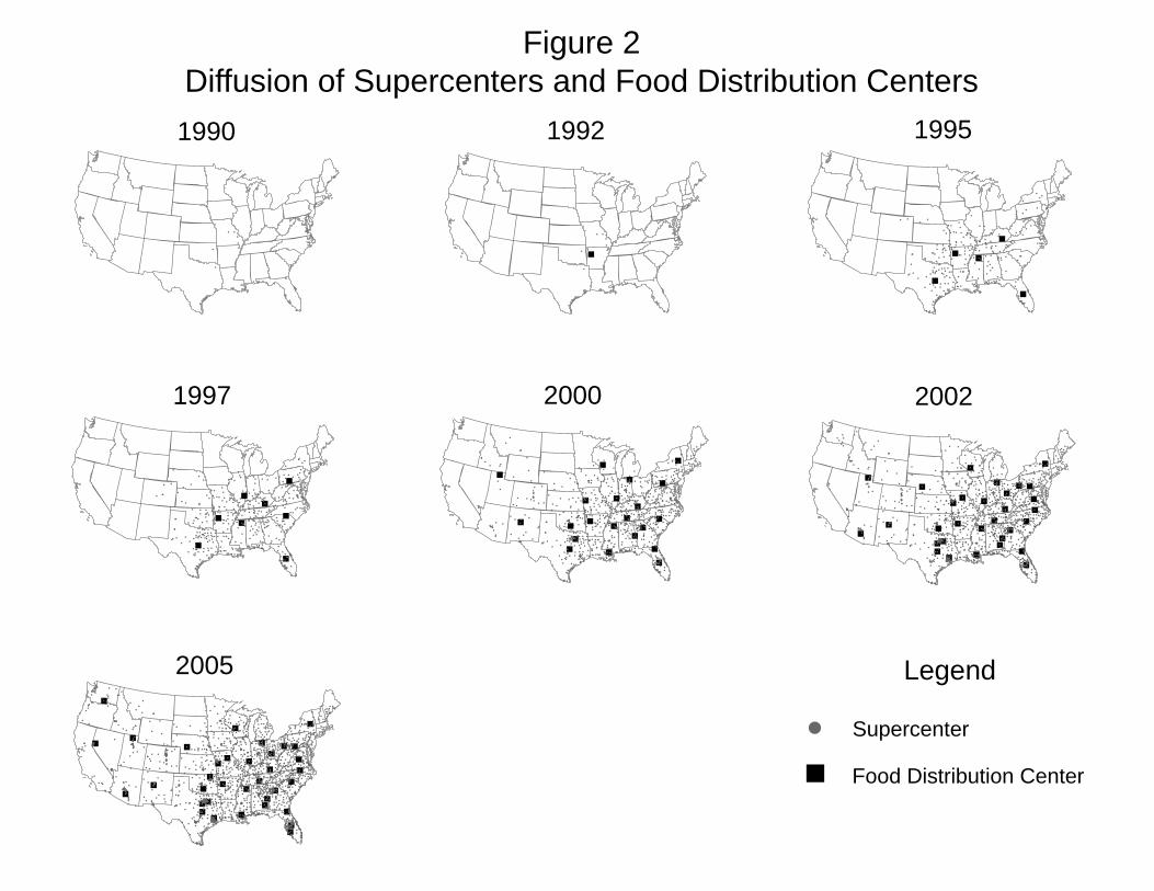
2005

"

"

"

"

""

"

"

"

"

"

"

"

"

"

"

"

"

"

"

"

! !

!!!

!

!

!

!

!

!

!

! !

!

!

!

!

!

!

!

!

!

!

!

!

!

!

!

!

!

!

!!

!!

!

!

!

!

!

!

!

!

!

!

!

!

!

!

!

!

!

!

!

!

!

!

!

!

!

!

!

!!

!

!

!

!

!

!

!

!

!

!

!

! !

!

!

!!!

!

!

!

!

!

!

!

!

!

!

!

!!

!

!

!

!

!

!

!

!

!

!

!

!

!

!

!

!

!!

!

!

!

!

!

!

!

!!

!

!!

!

!

!

!!

!

!

!

!

!

!

!

!!

!

!

!

!

!

!

!

!

!

!

!

!

!!

!

!

!!

!

!

!

!

!

!

!

!

!

!

!

!

!

!

!

!

!

!

!

!

!

!

!

!

!

!

!

!

!

!

!

!

!

!

!

!

! !! !

!

!

!!

!

!

!

!

!

!

!

!

!

!

!

!

!

!

!

!

!!

!

!

!

!!

!

!

!

!

!

!

!

!

!

!

!

!

!!

!

!

!

!

!

!!

!

!

!

!

!

!

!

!

!

!!

!

!

!

!

!

!

!

!

!

!

!

!

!

!

!

! !

!

!!!

!

!

!

!

!

!

!

!

!

!!

!!

!

!

!

!

!

!

!

!

!

! !!

!

!

!

!!

!

!!

!!!

!

!

!

!

!

!

!

!

!

!

!

!

!

!!

!

!

!

!

!

!

!

!

!

!

!

!!

!

!

!

!

!

!

!

!

!

!

!

!

!

!

!

!

!

!

!

!

!

!

!

!

!

!

!

! !

!

!

!

!

!

!

!

!

!

!

!

!

!

!

!

!

!

!

!

!

!

!!

!

!

!

!

!

!

!

!

!

!

!

!

!!

!

!

!

!

!!

!

!

!

!!

!

!

!

!

!!

!

!

! !

!

!

!

!

!

!

!!

!

!

!

!

!

!

!

!

!

!

!

!

!

!

!

!

!

!

!

!

!

!

!

!

!

!!

!

!

!

!

!

!

!

!

!

!

!

!

!

!

!

!!

!

!

!

!

!

!

!

!

!

!

!

!

!

!

!

!

!

!

!

!

!

!

!

!

!

!

!

!

!

!

!

!

!

!

!

!

!

!

!

!

!

!

!

!

!

!

!

!

!

!

!

!!

!

!

!

!!

!

!

!

!

!

!

!

!

!

!

!

!

!

!

!

!

!

!

!

!

!

!

!

!

!

!

!

!

!

!

!

!

!

!

!

!

!

!

!

!

!

!

!

!

!

!!!

!

!

!

!

!

!

!

!

!

!

!

!

!

!

!

!

!

!

!!

!

!

!

!

!

!

!

!

!

!

!

!

!

!

!

!

!

!

!!

!

!

!

!

!

!

!

!

!

!

!

!

!

!

!

!

!

!

!

!

!

!

!

!

!

!

!

!

!

!

!

!

!

!

!

!

!

!

!

!!

!

!

!

!

!

!

!

!

!

!

!

!

!

! !

!

!

!!

!

!

!

!

!

!

!

!

!

!

!

!

!

!

!

!

!

!

!

!

!

!

!

!

!

!!

!

!

!

!

!

!

!

!

!

!

!

!

!

!

!

!

!

!

!

!

!

!

!

!

!

!

!

!

!

!!

!

!

!

!

!

!

!

!

!

!

!

!

!

!!!!

!

!

!

!

!

!

!

!

!

!

!

!

!

!

!

!

!

!

!!

!

!

!

!

!

!

!

!

!

!

!

!

!

!

!!

!

!!

!

!

!

!

!!

!

!

! !!

!

!

!

!

!

!!

!

!

!

!

!!

!

!

!

!

!

!

!

!

!

!

!

!

!

!!

!

!

!

!

!

! !

!

!

!

!

!

!

!

!

!

!

!

!

!

!

!

!

!

!

!

!

!

!

!

!

!

!

!

"

"

"

"

"!!

!

!! !

!

!

!

!

!

!

!!

!

!

!

!

!

!

!

!

! !

!

!

!

!

!

!

!

!

!

!

!

!!

!

!

! !

!

!!!

!

!

! !

!

!

!

!

!

!

!

!

!

!

!!

!

!

!

!

!

!

!

!

!

!

!

!

!

!

!

!

!

!

!

!

!

!

!

!

!

!

!

!

!! !!

!

!

!

!!

!

!

!

!

!!

!

!

!

!

!

!

!

!

!

!

!

!

!!

!

!

!

!

! !

!!

!

!

!

!

!

!!

!

!!

!

!

!

!

!

!

!

!

!

!

!

!

!

!

!

!

!

!

!

!

!

!

!

! !

!

!

!

!

!

!

!

!

!

!

!!

! !

!

!

!

!

!

!

!

!!

!

!

!

!!

!

!

!

!

!

!

!

!!

!!

!

!

!

!

!

!

!

!

!

!

!

!

!

!

!

!

!

!

!

!

!

!

!

!

!

2000

19951990

Figure 2Diffusion of Supercenters and Food Distribution Centers

Legend

! Supercenter

" Food Distribution Center

"

!

!

!

!!

!

!

!

"

"

"

"

""

"

"

! !

!!

!

!

!! !

!

!

!

!

!

!

!

!!

!

!!

!

!

!

!

!

!

!

!

!

! !

!

!

!

!

!

!

!

!

!

!

!

!

!!

!

!

!

!

!

!

! !

!!!

!

!

!

!

!

!!

!

!

!!

!

!

!

!

!

!

!

!

!

!

!!

!

!

!

!

!

!

!

!

!

!

!

!

!

!

!

!

!

!

!

!

!

!

!

!

!

!

!

!

!

!

!

!

!

!

!

!

!

!

!

!

!

!

!

!

!

!

!! !!

!

!

!!

!

!

!

!

!

!

!

!

!

!

!

!

!

!

!

!!

!

!

!

!

!

!

!

!

!

!

!

!

!

!

!

!!

!

!

!

!

!

!!

!

!

!

!

!

!

!

!

!

! !

!

!!!

!

!

!

!

!

!

!

!

!

!

!

!! !

!

!!

!

!!

!!!

!

!

!

!

!

!

!

!

!

!

!

!

!

!

!

!

!

!

!

!

!!

!

!

!

!

!

!

!

!

!

!

!

!

!

!

!

!

!

!

!

!

!

!

!

!

!

!

!

!

!

!

!

!

!

!

!

!!

!

!

!

!

!

!!

!

!

!!

! !

!

!

!!

!

!

!

!

!

!

!

!

!

!

!

!

!

!

!

!

!

!

!

!

!

!

!

!

!

!

!

!

!

!

!

!

!

!

!

!

!

!

!

!

!

!

!

!

!

!

!

!

!

! !

!

!

!

!

!

!

!

!

!

!

!

!

!!

!

!!!

!

!

!

!

!

!

!

!

!!

!

!

!

!

!

!

!

!

!

!

!

!

!

!

!

!

!

!

!

!

!

!

!

!

! !

!

!

!

!

!

!

!

!

!

!

!

!

!

!

!

!

!

!

!

!

!!

!

!!

!

!

!

!!

!

!

"

"

"

"

""

"

"

"

"

"

"

"

"

"

"

"

"

"

"

""

"

""

"

"

"

" "

"

! !

!

!

!!

!

!

!!

!

!

!

!

! !

!

!

!

!

!

!

!

!

!

!

!

!

!

!

!

!

!

!

!

!

!

!

!

!!

!!

!

!

!

!

!

!

!

!

!

!

!

!

!

!

!

!

!

!

!

!

!

!

!

!

!

!

!

!

!

!!

!

!

!

!

!

!

!

!

!

!

!

!

! !

!

!

!!!

!

!

!

! !

!

!

!

!

!

!

!

!

!!

!

!

!!

!

!

!

!

!

!

!

!

!

!

!

!

!

!

!

!

!

!!

!

!

!

!

!

!

!

!!

!

!!

!

!

!

!!

!

!

!

!

!

!

!

!

!

!

!

!

!

!

!

!

!

!

!

!

!

!

!

!

!

!

!!

!

!!

!

!!

!

!

!

!

!

!

!

!

!

!

!

!

!

!!

!

!

!

!

!

!

!

!

!

!

!

!

!

!

!

!

!

!

!

!

!

!

!

!

! !! !

!

!

!!

!

!

!

!

!

!!

!

!

!

!

!

!

!!

!

!

!

!

!

!

!

!

!

!

!

!

!

!!

!

!

!

!!

!

!

!

!

!

!

!

!!

!

!

!

!

! !!

!

!

!

!

!

!

!

!

!

!

!

!

!

!

!

!

!

!

!

!

!!

!

!

!

!

!

!

!

!

!

!

!

!

!

!

!

!

!

!

!

!

!!

!

!

!

!

!

!!!

!

!

!

!

!

!

!

!

!

!

!

!!

!!

!

!

!

!

!

!

!

!

!

! !!

!

!

!

!

!

!

!

!!

!!!

!!

!

!

!

!!

!

!

!

!

!

!

!

!

!

!

!

!!

!

!

!

!

!

!

!

!

!

!

!

!

!!

!

!

!

!

!

!

!

!

!

!

!

!

!

!

!

!

!

!

!

!

!

!

!

!

!

!

!

!

!

!

!

!

!

!

!

!

!

! !

!

!

!

!

!

!

!

!

!

!

!

!

!

!

!

!

!

!

!

!

!

!

!

!

!

!

!

!!

!

!

!

!

!

!

!

!

!

!

!

!

!

! !

!

!!

!

!

!

!

!

!

!!

!

!

!

!!

!

!

!

!

!

!

!!

!

!

!

!

!

! !

!

!

!

!!!

!

!

!

!

!!

!

!

!

!

!

!

!

!

!

!

!

!!

!

!

!

!

!

!

!

!

!

!

!

!

!

!

!

!

!

!

!

!!

!

!

!

!

!

!

!

!

!

!

!

!

!

!

!

!

!

!

!!

!

!

!

!

!

!

!

!

!

!

!

! !

!

!

!

!

!

!

!

!

!

!

!

!

!

!

!

!

!

!

!

!

!

!

!

!

!

!

!

!

!

!

!

!

!

!

!

!!

!

!

!

!

!

!

!

!

!

!

!

!

!

!

!

!

!

!

!

! !

!

!

!

!

!

!

!

!

!

!

!

!

!

!

!

!

!

!

!

!

!

!

!

!

!

!

!!

!

!

!

!

!

!

!

!

!

!

!

!

!

!

!

!

!

!

!

!

!

!

!

!

!

!

!

!

!

!

!

!

!

!

!

!

!!

!

!

!

!

!

!

!

!

!

!

!

!

!

!

!

!

!

!

!

!

!

!

!

!

!

!

!

!

!!!

!

!

!

!

!

!

!

!

!

!

!

!

!

!

!

!

!

!

!

!

!

!

!

!

!

!

!

!

!

!

!!!

!

!

!

!

!!

!!

!

!

!

! !

!

!

!

!

!!

!

!

!

!!

!

!

!

!

!

!

!

!

!

!

!

!

!

!

!!

!

!

!

!

!

!

!

!

!

!

!

!

!

!

!

!

!

!

!

!

!

!

!

!

!

!

!

!

!

!

!

!

!

!

!

!

!

!

!

!

!

!

!

!

!

!

!

!

!

!

!

!

!

!

!

!

!

!

!

!

!

!

!

!

!

!

!

!

!

!

!

!

!

!

!

!

!

!

!

!

!

!

!

!

!

!

!

!

!

!

!

!

! !

!

!

! !

!!

!

!

!

!

!

!

!

!

!

!

!

!

!

!

!

!

!

!

!

!

!

!

!

!

!

!

!

!

!

!!

!!

!

!

!

!

!

!

!

!

!

!

!

!

!

!

!

!

!

!

!

!

!

!

!

!

!

!

!

!

!

!

!

!

!

!!

!

!

!

!

!

!

!

!

!

!

!

!

!

!

!!!!

!

!

!

!

!

!

!

!

!

!

!

!

!

!

!

!

!

!

!

!!

!

!

!

!

!

!

!

!

!

!

!

!

!

!

!

!

!!

!

!!

!

!

!

!

!!

!

!

! !!

!

!

!

!

!

!

!!

!

!

!

!

!!

!

!

!

!

!

!

!

!

!

!

!

!

!

!

!!

!

!

!

!

!

!

!

! !!

!

!

!!

!

!

!

!

!

!!

!

!

!

!

!

!

!

!

!

!

!

!

!

!

!

!

!

!

!

!

!

!

!

!

!

!

!

!

!

!

!!

!

!

!

!

!

!

!

!

!

!!

!!

!

!

! !

!

!

!

!

!!

!

!

!

!

!

!

!

!

!

!

!

!

!

!

!

!

!

!

!

!

!

!

!

!

!

!

!

!

!

!

!

!

!

!

!

!!

!

!

!

!

!

!

!

!

! !

!

!

!

!

!

!

!

!

!

!

!

!

!

!

!

!

!

!

!

!

!

!

!

!

!

!

!

1997

1992

2002

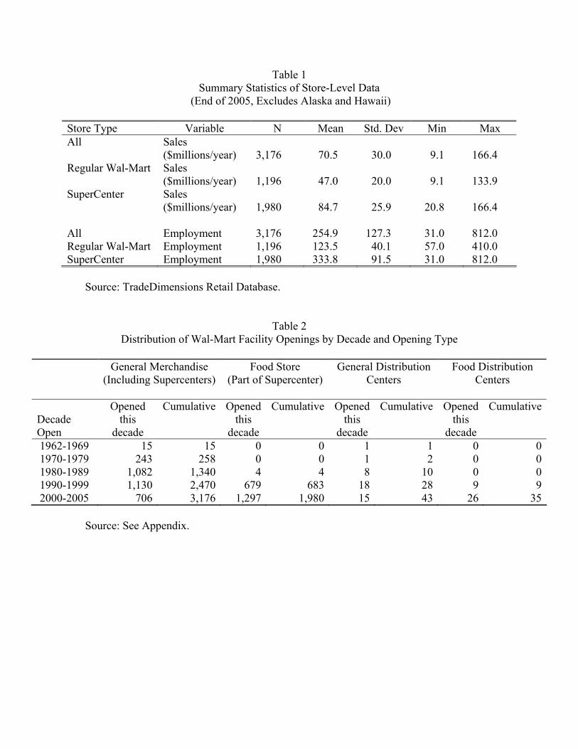
Table 1 Summary Statistics of Store-Level Data

(End of 2005, Excludes Alaska and Hawaii)

Store Type Variable N Mean Std. Dev Min Max All Sales

($millions/year) 3,176 70.5 30.0 9.1 166.4 Regular Wal-Mart Sales

($millions/year) 1,196 47.0 20.0 9.1 133.9 SuperCenter Sales

($millions/year) 1,980 84.7 25.9 20.8 166.4 All Employment 3,176 254.9 127.3 31.0 812.0 Regular Wal-Mart Employment 1,196 123.5 40.1 57.0 410.0 SuperCenter Employment 1,980 333.8 91.5 31.0 812.0

Source: TradeDimensions Retail Database.

Table 2 Distribution of Wal-Mart Facility Openings by Decade and Opening Type

General Merchandise (Including Supercenters)

Food Store (Part of Supercenter)

General Distribution Centers

Food Distribution Centers

Decade Open

Opened this

decade

Cumulative Opened this

decade

Cumulative Opened this

decade

Cumulative Opened this

decade

Cumulative

1962-1969 15 15 0 0 1 1 0 0 1970-1979 243 258 0 0 1 2 0 0 1980-1989 1,082 1,340 4 4 8 10 0 0 1990-1999 1,130 2,470 679 683 18 28 9 9 2000-2005 706 3,176 1,297 1,980 15 43 26 35

Source: See Appendix.

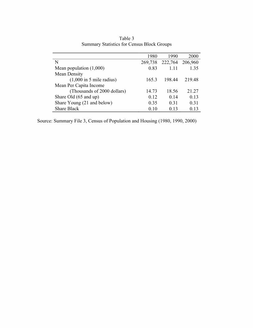
Table 3

Summary Statistics for Census Block Groups

1980 1990 2000 N 269,738 222,764 206,960 Mean population (1,000) 0.83 1.11 1.35 Mean Density (1,000 in 5 mile radius) 165.3 198.44 219.48 Mean Per Capita Income (Thousands of 2000 dollars) 14.73 18.56 21.27 Share Old (65 and up) 0.12 0.14 0.13 Share Young (21 and below) 0.35 0.31 0.31 Share Black 0.10 0.13 0.13

Source: Summary File 3, Census of Population and Housing (1980, 1990, 2000)

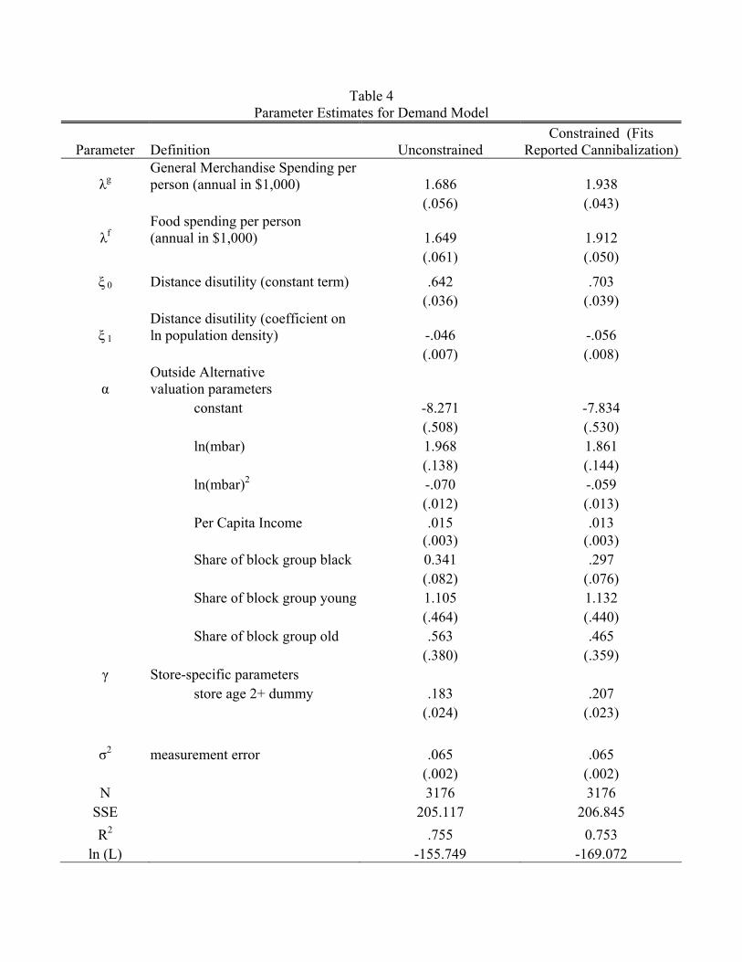
Table 4 Parameter Estimates for Demand Model

Parameter Definition Unconstrained Constrained (Fits

Reported Cannibalization)

λg General Merchandise Spending per person (annual in $1,000) 1.686 1.938

(.056) (.043)

λf Food spending per person (annual in $1,000) 1.649 1.912

(.061) (.050)

ξ 0 Distance disutility (constant term) .642 .703 (.036) (.039)

ξ 1 Distance disutility (coefficient on ln population density) -.046 -.056

(.007) (.008)

α Outside Alternative valuation parameters

constant -8.271 -7.834 (.508) (.530) ln(mbar) 1.968 1.861 (.138) (.144) ln(mbar)2 -.070 -.059 (.012) (.013) Per Capita Income .015 .013 (.003) (.003) Share of block group black 0.341 .297 (.082) (.076) Share of block group young 1.105 1.132 (.464) (.440) Share of block group old .563 .465 (.380) (.359) γ Store-specific parameters store age 2+ dummy .183 .207 (.024) (.023)

σ2 measurement error .065 .065 (.002) (.002) Ν 3176 3176

SSE 205.117 206.845

R2 .755 0.753 ln (L) -155.749 -169.072

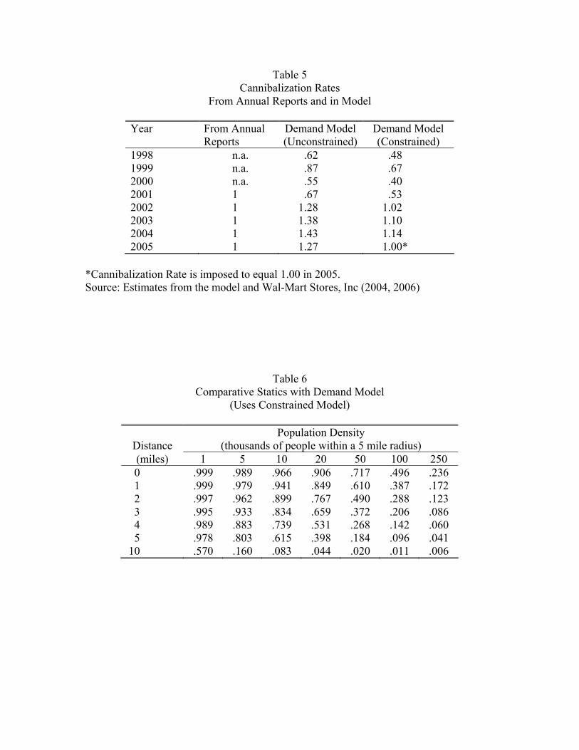
Table 5 Cannibalization Rates

From Annual Reports and in Model

Year From Annual Reports

Demand Model (Unconstrained)

Demand Model (Constrained)

1998 n.a. .62 .48 1999 n.a. .87 .67 2000 n.a. .55 .40 2001 1 .67 .53 2002 1 1.28 1.02 2003 1 1.38 1.10 2004 1 1.43 1.14 2005 1 1.27 1.00*

*Cannibalization Rate is imposed to equal 1.00 in 2005. Source: Estimates from the model and Wal-Mart Stores, Inc (2004, 2006)

Table 6 Comparative Statics with Demand Model

(Uses Constrained Model)

Distance Population Density

(thousands of people within a 5 mile radius) (miles) 1 5 10 20 50 100 250 0 .999 .989 .966 .906 .717 .496 .236 1 .999 .979 .941 .849 .610 .387 .172 2 .997 .962 .899 .767 .490 .288 .123 3 .995 .933 .834 .659 .372 .206 .086 4 .989 .883 .739 .531 .268 .142 .060 5 .978 .803 .615 .398 .184 .096 .041

10 .570 .160 .083 .044 .020 .011 .006

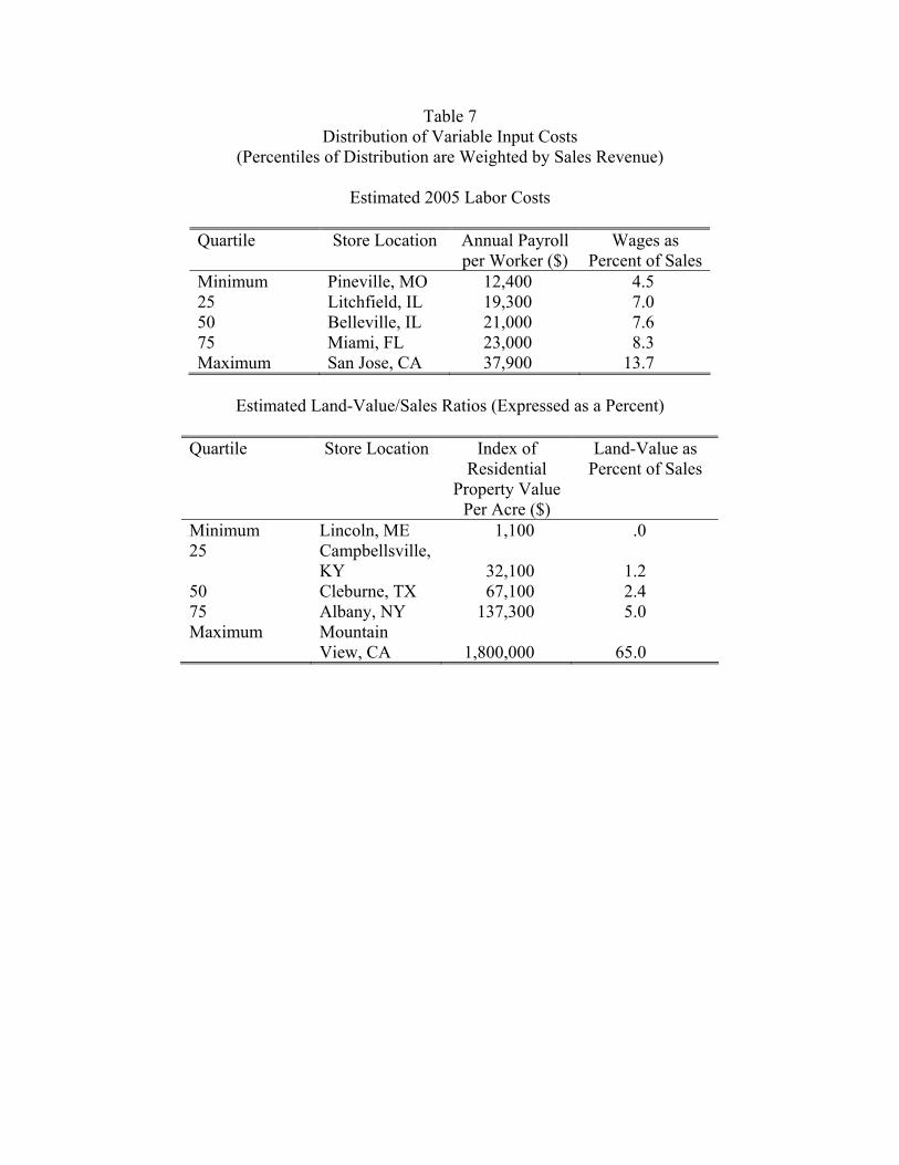
Table 7 Distribution of Variable Input Costs

(Percentiles of Distribution are Weighted by Sales Revenue)

Estimated 2005 Labor Costs

Quartile Store Location Annual Payroll per Worker ($)

Wages as Percent of Sales

Minimum Pineville, MO 12,400 4.5 25 Litchfield, IL 19,300 7.0 50 Belleville, IL 21,000 7.6 75 Miami, FL 23,000 8.3 Maximum San Jose, CA 37,900 13.7

Estimated Land-Value/Sales Ratios (Expressed as a Percent)

Quartile Store Location Index of

Residential Property Value

Per Acre ($)

Land-Value as Percent of Sales

Minimum Lincoln, ME 1,100 .0 25 Campbellsville,

KY 32,100 1.2 50 Cleburne, TX 67,100 2.4 75 Albany, NY 137,300 5.0 Maximum Mountain

View, CA 1,800,000 65.0

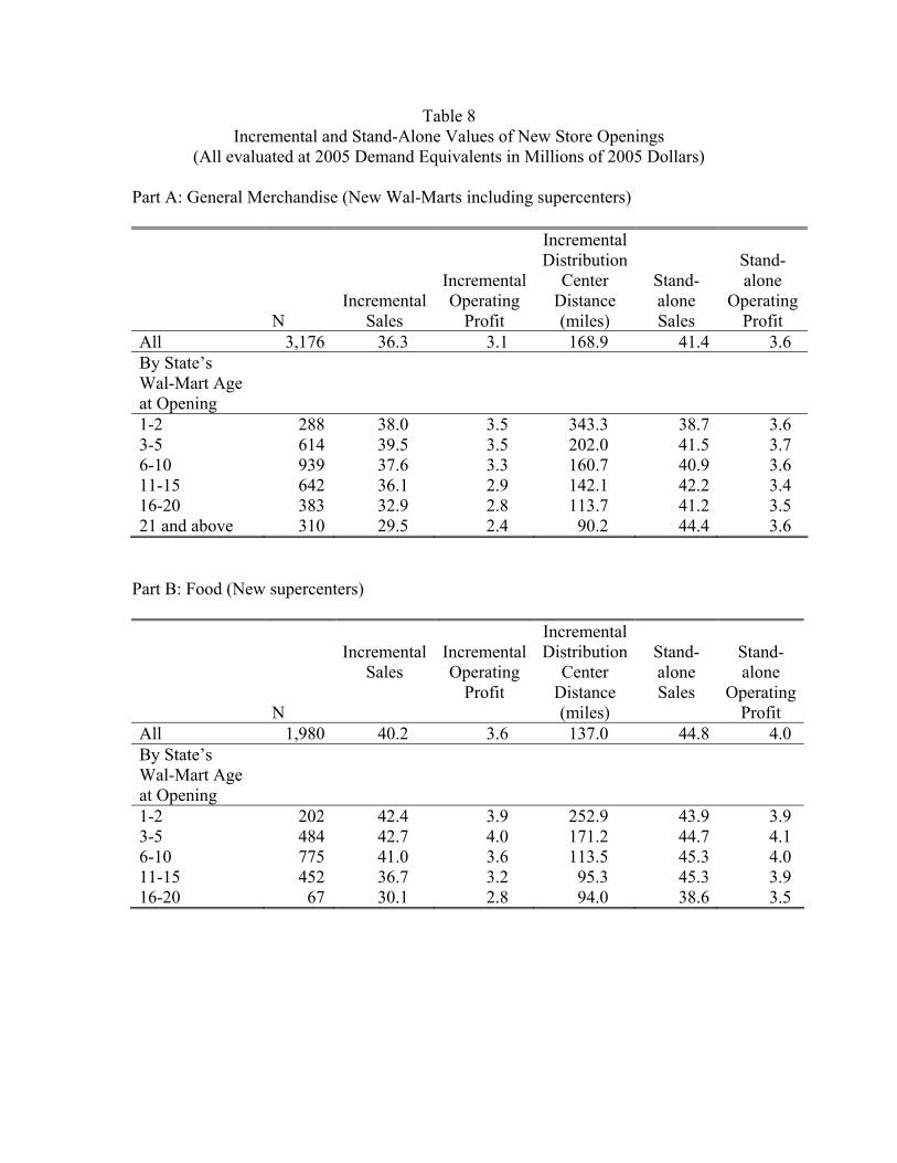
Table 8 Incremental and Stand-Alone Values of New Store Openings

(All evaluated at 2005 Demand Equivalents in Millions of 2005 Dollars)

Part A: General Merchandise (New Wal-Marts including supercenters)

N Incremental

Sales

Incremental Operating

Profit

Incremental Distribution

Center Distance (miles)

Stand-alone Sales

Stand-alone

Operating Profit

All 3,176 36.3 3.1 168.9 41.4 3.6 By State’s Wal-Mart Age at Opening

1-2 288 38.0 3.5 343.3 38.7 3.6 3-5 614 39.5 3.5 202.0 41.5 3.7 6-10 939 37.6 3.3 160.7 40.9 3.6 11-15 642 36.1 2.9 142.1 42.2 3.4 16-20 383 32.9 2.8 113.7 41.2 3.5 21 and above 310 29.5 2.4 90.2 44.4 3.6

Part B: Food (New supercenters)

N

Incremental Sales

Incremental Operating

Profit

Incremental Distribution

Center Distance (miles)

Stand-alone Sales

Stand-alone

Operating Profit

All 1,980 40.2 3.6 137.0 44.8 4.0 By State’s Wal-Mart Age at Opening

1-2 202 42.4 3.9 252.9 43.9 3.9 3-5 484 42.7 4.0 171.2 44.7 4.1 6-10 775 41.0 3.6 113.5 45.3 4.0 11-15 452 36.7 3.2 95.3 45.3 3.9 16-20 67 30.1 2.8 94.0 38.6 3.5

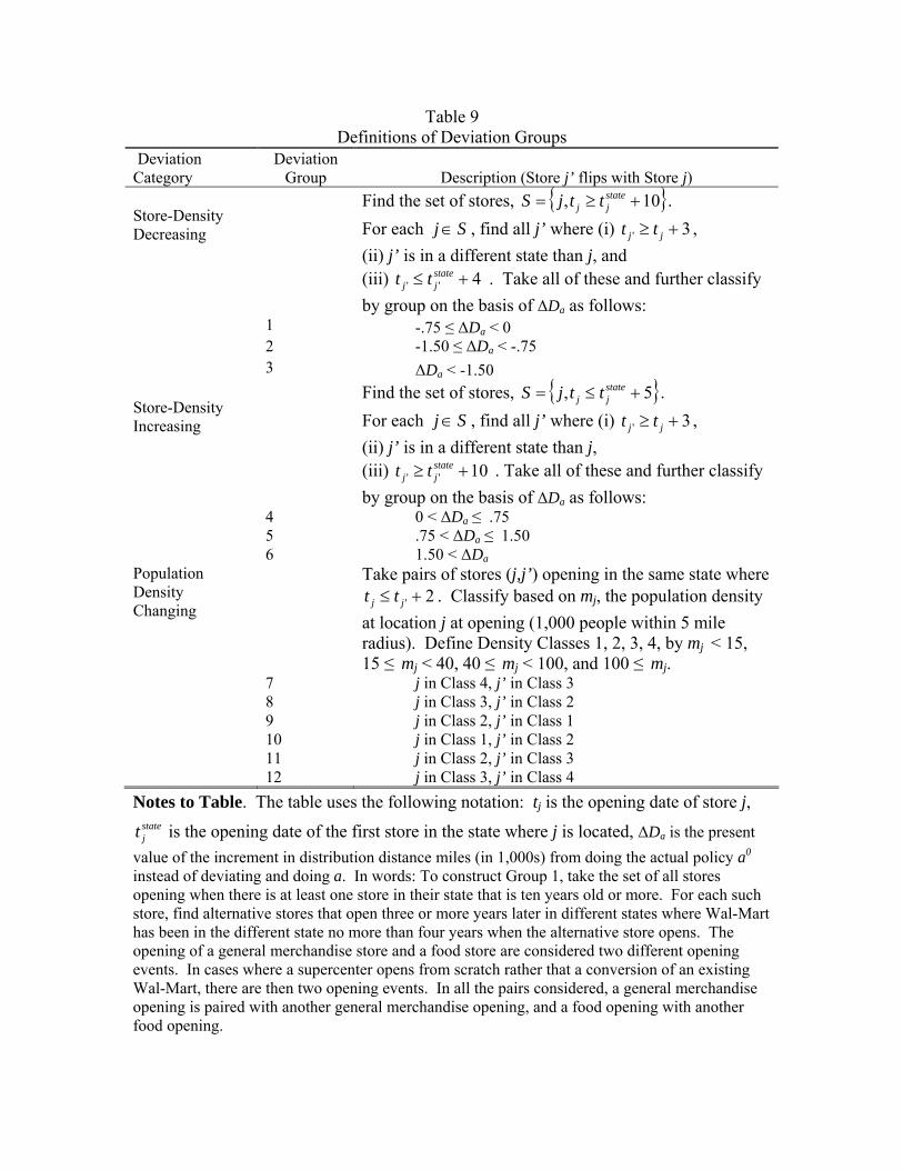
Table 9 Definitions of Deviation Groups

Deviation Category

Deviation Group Description (Store j’ flips with Store j)

Store-Density Decreasing

Find the set of stores, 10, statejj ttjS .

For each Sj , find all j’ where (i) 3' jj tt ,

(ii) j’ is in a different state than j, and (iii) 4'' state

jj tt . Take all of these and further classify

by group on the basis of ΔDa as follows: 1 -.75 ≤ ΔDa < 0 2 -1.50 ≤ ΔDa < -.75 3 ΔDa < -1.50

Store-Density Increasing

Find the set of stores, 5, statejj ttjS .

For each Sj , find all j’ where (i) 3' jj tt ,

(ii) j’ is in a different state than j, (iii) 10'' state

jj tt . Take all of these and further classify

by group on the basis of ΔDa as follows: 4 0 < ΔDa ≤ .75 5 .75 < ΔDa ≤ 1.50 6 1.50 < ΔDa Population Density Changing

Take pairs of stores (j,j’) opening in the same state where 2' jj tt . Classify based on mj, the population density

at location j at opening (1,000 people within 5 mile radius). Define Density Classes 1, 2, 3, 4, by mj < 15, 15 ≤ mj < 40, 40 ≤ mj < 100, and 100 ≤ mj.

7 j in Class 4, j’ in Class 3 8 j in Class 3, j’ in Class 2 9 j in Class 2, j’ in Class 1 10 j in Class 1, j’ in Class 2 11 j in Class 2, j’ in Class 3 12 j in Class 3, j’ in Class 4

Notes to Table. The table uses the following notation: tj is the opening date of store j, statejt is the opening date of the first store in the state where j is located, ΔDa is the present

value of the increment in distribution distance miles (in 1,000s) from doing the actual policy a0 instead of deviating and doing a. In words: To construct Group 1, take the set of all stores opening when there is at least one store in their state that is ten years old or more. For each such store, find alternative stores that open three or more years later in different states where Wal-Mart has been in the different state no more than four years when the alternative store opens. The opening of a general merchandise store and a food store are considered two different opening events. In cases where a supercenter opens from scratch rather that a conversion of an existing Wal-Mart, there are then two opening events. In all the pairs considered, a general merchandise opening is paired with another general merchandise opening, and a food opening with another food opening.

Table 10 Summary Statistics of Deviations by Deviation Group

Deviation Group

Brief Description of Group

Number of

Deviations Mean Values Δ~

(millions of 2005 dollars)

ΔD (thousands

of miles)

ΔF1 (log

popden)

ΔF2

(log popden2)

Store-Density Decreasing

1 -750 ≤ ΔD < 0 64,920 -2.7 -0.4 -0.6 -3.02 -1500 ≤ ΔD < -750 61,898 -3.6 -1.1 -1.5 -9.03 ΔD<-1500 114,588 -4.7 -3.0 -3.4 -22.2

Store-Density Increasing

4 0 < ΔD ≤ 750 158,208 3.0 0.3 -1.9 -17.25 750 < ΔD ≤ 1500 34,153 3.7 1.0 -3.6 -28.96 1500 <ΔD 16,180 5.9 2.1 -4.8 -37.7

Population-Density Changing

7 Class 4 to Class 3 7,048 1.2 0.0 3.2 31.18 Class 3 to Class 2 10,435 3.7 0.0 3.4 25.79 Class 2 to Class 1 14,399 5.3 -0.1 3.5 19.310 Class 1 to Class 2 12,053 -2.4 0.0 -3.4 -19.311 Class 2 to Class 3 14,208 0.6 -0.1 -3.9 -29.412 Class 3 to Class 4 14,877 2.5 0.0 -4.6 -44.9 All

Weighted Mean 522,967 -0.2 -0.6 -2.1 -15.6

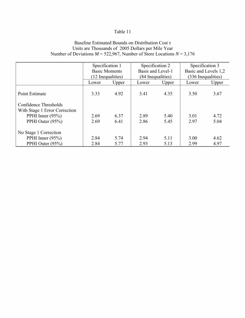
Table 11

Baseline Estimated Bounds on Distribution Cost τ Units are Thousands of 2005 Dollars per Mile Year

Number of Deviations M = 522,967, Number of Store Locations N = 3,176

Specification 1 Basic Moments (12 Inequalities)

Specification 2 Basis and Level-1 (84 Inequalities)

Specification 3 Basic and Levels 1,2

(336 Inequalities) Lower Upper Lower Upper Lower Upper

Point Estimate 3.33 4.92 3.41 4.35 3.50 3.67 Confidence Thresholds

With Stage 1 Error Correction PPHI Inner (95%) 2.69 6.37 2.89 5.40 3.01 4.72 PPHI Outer (95%) 2.69 6.41 2.86 5.45 2.97 5.04 No Stage 1 Correction PPHI Inner (95%) 2.84 5.74 2.94 5.11 3.00 4.62 PPHI Outer (95%) 2.84 5.77 2.93 5.13 2.99 4.97

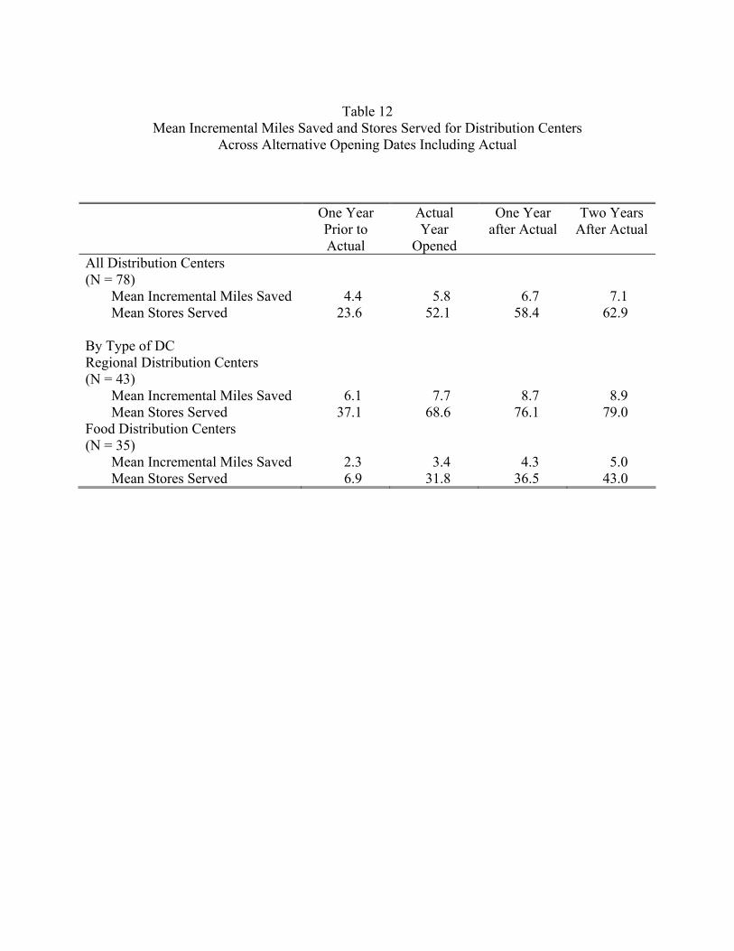
Table 12

Mean Incremental Miles Saved and Stores Served for Distribution Centers Across Alternative Opening Dates Including Actual

One Year Prior to Actual

Actual Year

Opened

One Year after Actual

Two Years After Actual

All Distribution Centers (N = 78) Mean Incremental Miles Saved 4.4 5.8 6.7 7.1 Mean Stores Served 23.6 52.1 58.4 62.9 By Type of DC Regional Distribution Centers (N = 43) Mean Incremental Miles Saved 6.1 7.7 8.7 8.9 Mean Stores Served 37.1 68.6 76.1 79.0 Food Distribution Centers (N = 35) Mean Incremental Miles Saved 2.3 3.4 4.3 5.0 Mean Stores Served 6.9 31.8 36.5 43.0

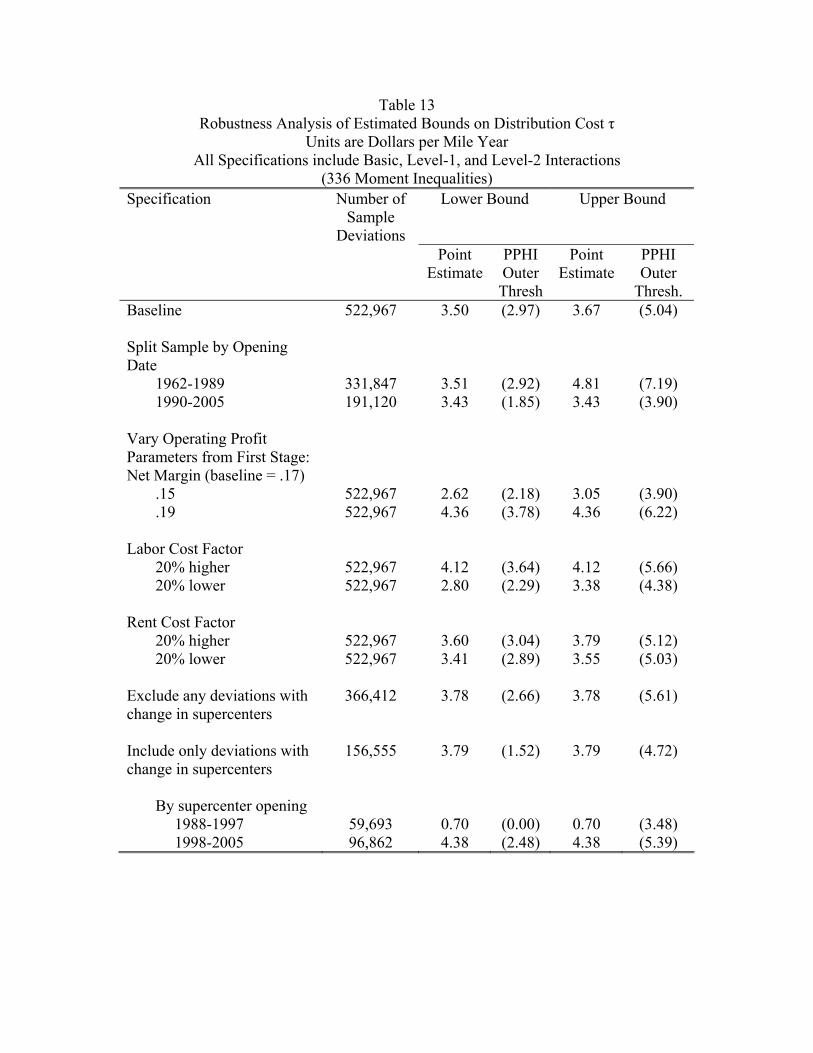
Table 13 Robustness Analysis of Estimated Bounds on Distribution Cost τ

Units are Dollars per Mile Year All Specifications include Basic, Level-1, and Level-2 Interactions

(336 Moment Inequalities) Specification

Number of Sample

Deviations

Lower Bound Upper Bound

Point Estimate

PPHI Outer Thresh

Point Estimate

PPHI Outer

Thresh. Baseline

522,967 3.50 (2.97) 3.67 (5.04)

Split Sample by Opening Date

1962-1989 331,847 3.51 (2.92) 4.81 (7.19) 1990-2005 191,120 3.43 (1.85) 3.43 (3.90) Vary Operating Profit Parameters from First Stage:

Net Margin (baseline = .17) .15 522,967 2.62 (2.18) 3.05 (3.90) .19 522,967 4.36 (3.78) 4.36 (6.22) Labor Cost Factor 20% higher 522,967 4.12 (3.64) 4.12 (5.66) 20% lower 522,967 2.80 (2.29) 3.38 (4.38) Rent Cost Factor 20% higher 522,967 3.60 (3.04) 3.79 (5.12) 20% lower 522,967 3.41 (2.89) 3.55 (5.03) Exclude any deviations with change in supercenters

366,412 3.78 (2.66) 3.78 (5.61)

Include only deviations with change in supercenters

156,555 3.79 (1.52) 3.79 (4.72)

By supercenter opening 1988-1997 59,693 0.70 (0.00) 0.70 (3.48) 1998-2005 96,862 4.38 (2.48) 4.38 (5.39)