TRADE VOLATILITY AND THE GATT/WTO:

DOES MEMBERSHIP MAKE A DIFFERENCE?

Abdur Chowdhury Department of Economics

College of Business Administration Marquette University

Xuepeng Liu Department of Economics & Finance

Kennesaw State University

Miao Wang Department of Economics

College of Business Administration Marquette University

M. C. Sunny Wong Department of Economics

University of San Francisco

TRADE VOLATILITY AND THE GATT/WTO:

DOES MEMBERSHIP MAKE A DIFFERENCE?

Using bilateral trade data for 210 countries over the period 1948-2003, this paper attempts to shed some light on the relationship between the WTO and members’ trade volatilities. We find that the trade among WTO members tends to be more stable than the trade outside the WTO, and there is strong evidence of interdependence of trade volatilities. The results show comovement of trade volatilities across all dyads in general, and much stronger comovement among WTO members than between WTO and non-WTO members. Such strong comovement implies that WTO member countries not only share the benefits of having an interdependent and more predictable trade system, but also share the risks of contagious world trade collapse as evidenced by the 2008 global financial crisis. In addition, we find that larger economies and countries covered by other types of integration agreements can do better in coping with such a type of contagion. Key words: trade volatility, WTO, gravity model, contagion, dyadic spatial volatility JEL classification: F02, F13, F14

1

1. Introduction

Globalization in the last few decades has generated an unprecedented increase in international

trade flows.1 While the advantages to this process are many, the rise in economic openness that

has accompanied globalization has also made countries more vulnerable to international

economic volatility, and to trade volatility in particular (see Rodrik, 1998, among others). Such

instability is a major cause for concern because in an open economy, volatility of trade can have

various adverse consequences. Specifically, such volatility can retard economic growth, deter

trade and investment, raise the cost of external borrowing, aggravate budget deficits, decrease

personal income security, and reduce public support for integration in the global economy.

These potential misfortunes have led policy makers around the globe to sound the alarm

against rising trade volatility. In this regard, researchers have recently recognized that

international organizations possess a number of unique features that work together to help states

manage international volatility (see, e.g., Marting and Simmons, 1998; Braumoeller, 2006). On

trade agreements in particular, Mansfield and Reinhardt (2008) find that the World Trade

Organization (WTO) and its predecessor, the General Agreement on Tariffs and Trade (GATT),

as well as preferential trading agreements (PTAs) 2 reduce trade volatility by constraining

member-states from introducing new trade barriers, diversifying the composition of trade and

foreign direct investment flows, and increasing transparency in policy, expectations and trade

standards and policy instruments. Rose (2005), on the other hand, shows that membership in the

GATT/WTO has no dampening effect on trade volatility.

Given the lack of a clear consensus on this important trade policy issue, our paper aims to

take this research forward by addressing several fundamental questions. First, does the

GATT/WTO reduce the bilateral trade volatility among WTO members? Second, how does the

bilateral trade volatility of WTO members co-vary with the volatilities of their trading partners,

depending on partners’ WTO membership? Third, how countries can cope with the contagion?

Only a few existing studies directly address the relationship between international

organization membership and trade volatility (Rose, 2005; Mansfield and Reinhardt, 2008), but

none of them analyzes the comovement of the trade among WTO members to our best

knowledge. Bilateral trade volatility between an importer and an exporter may depend not only

1 Between 1950 and 2005, the average annual growth rate of the volume of world exports was 6.2% (7.5% for manufacturers), compared with a GDP growth of 3.8% (WTO, 2007). 2 We use PTAs interchangeably with regional trade agreements (RTAs) in this paper.

2

on bilateral characteristics, but also on trade volatilities of other dyads. For example, volatility of

trade between the U.S. and Thailand depends not only on the GDP per capita of the U.S. and

Thailand (and other country level characteristics specific to this pair of countries), but also on

trade volatility between the U.S. and South Korea and the trade volatility between the Thailand

and Japan. In this paper, we include other dyads’ trade volatility as an additional determinant of

the trade volatility of a dyad of interest, along with other factors considered by previous studies.

If bilateral trade volatility is affected by trade volatility between other dyads (which is very

likely), omitting a measure of the multilateral dependence of trade volatility can lead to biased

estimated coefficients and invalid statistical inferences.

Our sample includes bilateral trade data for 210 countries over the period 1948-2003.

This is the most complete country coverage among available bilateral trade datasets. We link

different dyads by WTO membership, geographical distance between countries, and trade

relationship and create a spatial term of other dyads’ trade volatility, which is described in detail

in Section 3. We find that, with a spatial term of trade volatility in regressions, a dyad’s trade

volatility is lower when both partners are WTO members. More importantly, our results provide

strong evidence for interdependence of trade volatilities. We find comovement of trade

volatilities across all dyads in general, and such comovement is much stronger among WTO

members than that between WTO and non-WTO members. Our results are robust to different

measures of trade volatilities and different subsamples. The comovement of trade volatilities

among WTO members implies that member countries not only share the benefits of having an

interdependent and more predictable trade system, but also share the risks of contagious world

trade collapse as evidenced by the 2008 world financial crisis. Finally, we show that countries of

larger economic sizes can do better in coping with the contagion. Regional trade agreements

(RTAs), currency unions (CUs), and the General System of Preferences (GSP) among WTO

members help to diversify the risks and alleviate the contagion sourced from other WTO

members.

The rest of the paper is organized as follows. A review of the existing literature and the

theoretical underpinning of the two hypotheses considered in this paper are presented in Section

2. The methodology is presented in Section 3, and the regression results are discussed in Sections

4 and 5. The paper ends with concluding policy remarks in Section 6.

3

2. Literature Review and Theoretical Issues

The GATT/WTO is often recognized as among the most successful multilateral institutions in

the last six decades (Bagwell and Staiger, 2002; Bhagwati, 1999). The impressive annual growth

in world trade of 6.2% between 1950 and 2005 is often attributed to the visible role played by the

WTO in reducing barriers to trade through eight successive rounds of negotiations. In the

following, we review briefly the literature on the effects of trade and trade agreements on the

level and volatility of bilateral trade, as well as the adverse impact of trade volatility on

economic development.

Somewhat surprisingly, however, when Rose (2004) sets out to quantify the trade-

enhancing role of WTO membership in an econometric study of world trade based on the gravity

equation, he concludes that GATT/WTO has a limited role in the promotion of world trade. His

findings have sparked a growing body of literature. In response to Rose’s conclusions,

Subramanian and Wei (2007) show that the impact differs across countries and sectors because

of asymmetries within the GATT/WTO system. They demonstrate that the growth in trade flows

of the industrialized countries is higher than that in the developing countries that are also part of

the system, and the trade promoting effect of the GATT/WTO is stronger for some sectors than

others. Taking into account both formal GATT/WTO members and non-member participants,

Tomz et al. (2007) find that the GATT/WTO has had substantial positive effects on trade.3 All of

these papers cover only positive bilateral trade flows to study the trade effect of the WTO at the

intensive margin. Helpman et al. (2008) and Liu (2009) include both positive and zero bilateral

trade flows and show that the WTO has a strong effect at the extensive margin by creating new

trading relationship. A number of papers address Rose’s WTO puzzle from other aspects, but we

do not intend to be exhaustive here. Overall, these papers take a more optimistic view of the

WTO in promoting bilateral trade.

It is now generally accepted that the boost in international trade in the last several

decades has also led to more volatility and uncertainty in trade. A number of distinct economic

mechanisms are at play in the relationship between openness to trade and trade volatility

(Haddad et al. 2012). The overall effect is, however, ambiguous and needs to be identified

empirically. On one hand, as export earnings increase, the terms of trade can directly affect

3Tomz et al. (2007) argue that Rose’s analysis overlooks a large group of countries to which the trade agreement applied and classified them incorrectly as nonparticipants (non-member participants). This causes a downward bias in the estimated effect of GATT/WTO on trade.

4

output and growth in a major way. Declining demand overseas not only reduces export

shipments and harms producer revenues, but also can lead to falling prices and worsening terms

of trade. On the other hand, as a country’s export sector responds to overseas market conditions,

it becomes relatively less correlated with home market conditions. Because demand shocks at

home and overseas are only imperfectly correlated, this force tends to reduce overall volatility in

output. Moreover, outward orientation means that a country is more likely to export more

products to more markets – an international diversification. A country’s exports are similar to an

investment portfolio. Exporting one product to one foreign market is a very risky endeavor

because the exporting country is completely dependent on demand conditions in that one

importing country. Exporting multiple products to a range of foreign markets reduces this risk

through a diversification effect. However, there is a tension between international diversification

from outward orientation and the specialization that trade induces (Kellman and Shachmurove,

2011). Evidence suggests that specialization does not dominate until countries are well into the

high-income group. Although these mechanisms apply to trade in general, they also apply to

trade agreements such as the WTO with trade liberalization being their primary objective.

In comparison to the growing literature on the trade impact of WTO membership, the

number of papers looking at the impact of membership on trade volatility is scant. Rose (2005)

examines the hypothesis that membership in the GATT/WTO has increased the stability and

predictability of trade flows. Using a large data set covering bilateral trade flows between over

175 countries between 1950 and 1999, he finds little evidence that membership in the

GATT/WTO has a significant dampening effect on trade volatility. Mansfield and Reinhardt

(2008), on the other hand, assume that exposure to global markets increases terms of trade

volatility. Governments seek to insulate their economies from such instability through

membership in international trade institutions, particularly the WTO and PTAs. They

hypothesize that international institutions reduce trade volatility through three related

mechanisms. First, trade agreements reduce future volatility in trade-flows by ‘locking-in’ states’

existing trade commitments and deterring the erection of new protectionist barriers. Second,

trade-agreements increase policy transparency and promote policy convergence among member

states, which they argue reduces trade volatility by stabilizing the expectations of traders,

providing these actors with clearer avenues for trade dispute resolution and settlement. Third,

international trade institutions signal long-term predictability and low credit-risk environments to

5

international investors. This, in turn, reassures investors that governments will not engage in

predatory behaviors, increases FDI flows and shifts FDI composition more towards vertical and

export-platform FDI, and helps to diversify export portfolios, all of which decrease international

economic volatility. Using bilateral export data from 1951 through 2001, they provide support

for their arguments: PTAs and the WTO regime significantly reduce export volatility.

Finally, recent empirical studies have established that trade volatility harms countries

through several interrelated channels, justifying the importance of understanding the sources of

the volatility and policy instruments to cope with the volatility. Perhaps most notably, volatile

trade flows can significantly undermine a country’s domestic economic stability. In this regard,

trade volatility has been found to threaten workers’ employment and wages (Scheve and

Slaughter, 2004), reduce firm profits and market competitiveness (Aizenman, 2003), and depress

or destabilize economic growth (Rodrik, 1998, 1999; Kim, 2007).

The latter effect - that of trade volatility on aggregate economic growth - has been found

to be especially acute (Rodrik, 1998, 1999; Grimes, 2006). For example, in a multi-decade study

of New Zealand, Grimes reports that “approximately half the variance in annual GDP growth

over 45 years can be explained by the level and volatility of the terms of trade”, while others find

that these adverse effects of trade volatility may be even more severe for developing countries

(Blattman, Hwang and Williamson, 2007; Razin, Sadka and Coury, 2003). Second, in part as a

result of its harmful economic effects, trade volatility can also increase civil conflict. The harm

done to growth, investment, and employment by trade volatility lead to increased social and

distributional conflicts between groups and governments, especially in countries with weak

domestic institutions (Rodrik, 1999; Miguel et al., 2008; Hidalgo et al., 2010). Finally, because

trade volatility increases uncertainty, it also threatens the profitability of international commerce,

and hence, reduces the actual size of trade flows between countries (Mansfield and Reinhardt,

2008). Thus, trade instability poses a multitude of political and economic threats to societies and

governments.

Building on the existing literature, the goal of the current paper is to show that WTO

members not only benefit from growing international trade, but also share the risks and

volatilities. Specifically, we show that trade volatility co-moves among the dyads within the

WTO, but not so strongly between dyads within the WTO and those outside the WTO. This

finding can be driven by, but not limited to, the following factors. First, similar to Mansfield and

6

Reinhardt (2008), we find that the WTO reduces the volatility of the bilateral trade. If all the

bilateral trade within the WTO becomes less volatile, we should observe a comovement of trade

volatility under the WTO. In this case, our previous discussion on how trade openness and trade

agreements reduce trade volatility also applies. Second, if a WTO member lowers its MFN

tariffs, the lower tariffs should apply to all of the other WTO members according to the non-

discrimination clause, but not to non-WTO members. This may lead to a comovement within the

WTO, but not for the bilateral trade between members and non-members. Third, with increasing

global outsourcing and production fragmentation, the production can be more vertically

integrated among WTO members, which can in turn lead to the comovement of production and

trade volatility among WTO members.

3. Empirical Methodology

3.1 Baseline Empirical Specification and Data

Our empirical analysis uses a gravity model, which has been widely used to study the

determinants of bilateral trade volume. We start with a basic gravity-type specification as

follows:

Vol Mijt 0 1Bothinijt 'Z ijt, (1)

where Mijt represents the value of c.i.f. imports of country i from country j; Vol Mijt is the

volatility of Mijt, measured as a standardized deviation of imports from its predicted value.

Specifically,

Vol Mijt absln Mijt ln Mijt trend

ln Mijt trend

(2)

where ln Mijt trend is a predicted value of import of country i from country j modeled as a third

order polynomial in time trend and abs represents absolute value. Rose (2005) uses the standard

deviation of imports over mean value of imports over a certain period of time to measure trade

volatility. By comparison, our measure in equation (2) has a number of advantages. First, a de-

trended measure is more appropriate than a simple standard deviation when a country’s import

experiences a growing or a declining trend as the standard deviation can be large due to either a

volatile trade pattern or a large and steady growth or decline. Empirical studies need to capture

7

the former, not the latter. Second, our measure is less sensitive to missing observations. For

example, even if a country’s trade follows a smooth growth trajectory over time, the calculated

standard deviation can be large if many years of trade data are missing in between and only the

trade data of the very first years (of small values) and that of very last several years (of large

values) are observed. Third, our measure better preserves time variations in the sample, while the

standard deviation, if calculated over the entire sample period, has only one observation for a

dyad. For robustness checks, in addition to the volatility measure in equation (2), we also adopt

other measures including one similar to that in Rose (2005).

Following Tomz et al. (2007), Bothinijt is a dummy variable taking the value of one if

both importing (i) and exporting (j) countries are de facto WTO members (either formal

members or non-member participants) in year t and zero otherwise.; Z is a vector of other control

variables commonly chosen in a gravity model, including log value of real GDP of i and j

(lnGDPit and lnGDPjt), log value of real GDP per capita of i and j (lnGDPPCit and lnGDPPCjt ),

log value of the great-circle distance between i and j (lnDistij), log value of the geographical area

of i and j (lnAreai and lnAreaj), the number of landlocked countries in a pair (Landlockij = 0, 1,

or 2), the number of island nations in a pair (Islandij = 0, 1, or 2), whether the pair of countries

share a border (Borderij), whether i and j share a common language (ComLangij), whether i and j

share a common religion (ComReligij), whether country i has ever been a colony of j (Colonyij),

whether country i has ever been a colonizer of j (Colonizerij), whether i was currently a colony of

j in year t (CurColonyijt), whether i was currently a colonizer of j in year t (CurColonizerijt),

whether i and j belong to the same regional trading agreement in year t (RTAijt) or the same

currency union (CUijt), whether j offered GSP to i in year t (GSPijt), whether i and j are in a

formal alliance in year t (Allianceijt) and the military conflict intensity between i and j

(Hostilityij), and a remoteness measure. Country i’s remoteness is defined as the distance of

country i to the rest of the world weighted by all the other countries’ GDPs in year t (Remotejt).

The remoteness of a dyad ij (Remoteijt) is simply the sum of Remoteit and Remotejt.

In the following, we discuss the general and dyadic spatial lag models and a gravity

specification augmented with spatial terms.

3.2 Spatial Lag Model in General and Dyadic Spatial Effects

8

Spatial analysis recognizes the importance of geographical locations and distance in social

economic activities. Often, two spatial effects are tested - spatial dependence and spatial

heterogeneity. Spatial dependence occurs when the observation in location i is correlated with

observations in other locations j while spatial heterogeneity indicates that the functional form of

a model as well as coefficients in a regression can vary across different locations in space. As our

main interest is the comovement of trade volatilities, we will focus on spatial dependence,

specifically the spatial lag model, rather than spatial heterogeneity.

The essence of a basic spatial lag model is reflected in the first law of geography,

“[e]verything is related to everything else, but near things are more related than distant things”

(Tobler, 1970). Formally, we can state:

Y = Xβ + ρWY + ε (3)

where Y is an 1 vector of observations for a monadic cross-sectional sample with N units

(or across N locations); X is an matrix of explanatory variables; is a vector of M

coefficients. The term WY in equation (3) is called the spatially lagged dependent variable, with

W as an N N matrix measuring the connectivity between N number of yi and N number of yj .

For any yi , WY is a weighted average of all yj 's in neighboring locations or a lag of yi over

space. Consequently, equation (3) suggests that the variation in each observation of y is

explained by its dependence on the others. The sign and magnitude of ρ illustrate the impact of

the spatial lag on the dependent variable. If ρ is positive, an increase in spatially weighted y in all

other locations j (for all j ≠ i) is associated with an increase in yi . Conversely, if ρ is negative,

then an increase in spatially weighted y in all other locations j is associated with a decrease in yi .

For panel data with N units and T time periods, the weight matrix W becomes a block

diagonal matrix of NT NT with each block capturing a single year’s observations. With T time

periods, the weight matrix can be expressed as equation (4):4

(4)

4 The weight matrix W is also row-standardized so that each row sums to unity.

9

where Wt

0 wt ij wt ik wt ji 0 wt jk wt ki wt kj 0

with wt being a weight function for Tt ,,1 .

Each block matrix Wt is an N N symmetric matrix and entries of Wt connect two units among

i, j and k in year t. The diagonal elements of Wt are zeros to ensure that no observation of Y

predicts itself.

Dyadic Spatial Model

In our study, we have directed dyadic data with a source country and a target country in a dyad,

in which imports of country i from country j are treated differently from imports of country j

from country i.5 In a dyadic framework, spatial dependence implies that the interaction between

two units in a pair is explained by interactions between units in other pairs and such

interdependence becomes more complicated than in the monadic case. Neumayer and Plümper

(2010) systematically categorize the complex ways of modeling dependence with dyadic data.6

Following Neumayer and Plümper, we express a generic form of dyadic spatial lag model

(ignoring other explanatory variables in the model) in equation (5),

yijt wpqykmt ijt,ijkm (5)

where yijt is an observation with source country i and target country j at time t. For instance, yijt

can represent import of country i from country j in year t. Note that in this case the words

“source” and “target” are used to simply suggest that yij and yji are not identical and they do not

necessarily represent the direction of trade flows. To avoid confusion, we will use

importer/exporter rather than source/target country in most places in this paper. The wpq in

equation (5) is a weight determining the connectivity between dyads km and ij at time t, with

row-standardization where wpq 1 . Neumayer and Plümper (2010) have presented all

variations of equation (5) in their paper. We will describe two of the specifications applicable to

our study, namely the exporter specific contagion and the importer specific contagion. Interested

5 Distance between two countries is an example of undirected dyad information since distance from i to j is the same as distance from j to i. 6 In the trade literature, Egger and Larch (2008) is one of the earliest studies to consider a spatial relationship in the context of the contagion effects of RTA formation.

10

readers are referred to Neumayer and Plümper (2010) for an extensive discussion of all possible

specifications.

3.3 Augmented Specification with Spatial Measures of Trade Volatilities

We now include four spatial measures (Vs) in our model as controls to consider both the demand

and supply side of trade volatilities of “other pairs” as follows:

,04130211 ' ijtjtjttitiijt ZVVVVMVol (6)

where:

.

and,

,

,

0

1

0

1

ikkjtWTOnonjt

ikkjtWTOjt

jmimtWTOnonti

jmimtWTOti

MVolV

MVolV

MVolwV

MVolwV

These four measures on the right-hand side of equation (6) represent spatially lagged

import volatilities for any dyad ij the weighted average of import volatilities from other pairs

based on WTO membership. The first two measures of spatial lags, tiV 1 and tiV 0 , are importer

specific contagion spatial lag terms, representing the average volatility of i-m when the exporters

( ) are WTO and non-WTO members (represented by the subscripts 1 and 0), respectively.

They allow us to analyze how the volatility of imports of country i from country j is related to

the volatility of imports of country i from other exporting countries m, where m j . For

example, the volatility of imports of the U.S. from Thailand is correlated with the volatility of

imports of the U.S. from India or with the volatility of imports of the U.S. from Germany. The

weight wWTO equals one if country m is a WTO member and zero otherwise, and the weight

wnonWTO takes the value of one if country m is not a WTO member. As a result, Vi1t shows the

average volatility of imports of country i from other WTO member exporters (excluding j) in

year t. The term Vi0 t is an average volatility of imports of country i from other non-WTO

exporters (excluding j) in year t.

The next two spatial lags, V1 jt and V0 jt are exporter specific contagion terms,

representing the average trade volatility between k-j when the importers ( ) are WTO and

jm

ik

11

non-WTO members (represented by the subscripts 1 and 0), respectively. They allow us to

analyze how the volatility of imports of country i from country j may be influenced by the

volatility of imports of other importing countries k from the same exporting country j. This

suggests, for example, the volatility of imports of the U.S. from Thailand is influenced by the

volatility of imports of Germany from Thailand or by the volatility of imports of India from

Thailand. The weight WTO is one when the importing country k is a WTO member and zero if

not. The weight nonWTO equals one when the importing country k is a non-WTO member and

zero otherwise. As a result, the coefficient on V1 jt gives the average impact of volatility of

imports of WTO member importers from the exporter j on volatility of imports of i from j. The

coefficient on V0 jt shows the average impact of volatility of imports of non-WTO member

importers from the exporter j on the volatility of imports of i from j.

To better explore whether WTO members experience a convergence in trade volatility

among themselves, we restrict our sample to observations with both the exporter and the

importer being WTO members. Note that the exporter and importer specific contagion spatial

lags are still calculated based on all dyads in the whole sample and then we run regressions

including only dyads with both countries being de facto WTO members. As both the importer

and exporter are WTO members, the variable Bothin is dropped from the regressions based on

equation (6).7

7We note that one might attempt to include all the dyads in the regressions, and redefine the four spatial lag terms in theory as follows: (7)

where

Although it seems that we can estimate the coefficient of Bothin as well using the full sample, this specification in practice is equivalent to the WTO subsample regressions we run for Table 3. For example, the first term in

equation (7) takes a positive value only when all three countries (i, j, and m) are WTO members. For any dyad ij with neither i nor j being a WTO member, will have a missing value. As a result, all dyads with i and j not being

WTO members will be dropped from the estimation.

12

Figure 1 illustrates graphically how we define these spatial terms for dyad ij. Note that

when WTO membership is the sole weight to construct the spatial lags, and both countries i and j

are WTO members, the value of the exporter specific contagion term Vi0 t will be the same for an

importer (i) for a given year, not varying with exporting countries. Similarly, the importer

specific contagion term V0 jt will be the same for an exporter (j), regardless the exporters.

However, term is not importer i-specific for a given year because we leave country j out for

each dyad ij (i.e., m j). Similarly, V1 jt is not exporter j-specific either for a given year because

we leave country i out for each dyad ij ( k i).

4. Empirical Results

The data used in our analysis are from Liu (2009). As mentioned earlier, this sample covers 210

countries over the period 1948-2003 and, to the best of our knowledge, has the most complete

country coverage among available bilateral trade datasets. Summary statistics of the variables in

our model are provided in Table 1.

4.1 Baseline Regressions without Spatial Measures

Our baseline regression results on the effect of WTO membership on trade volatility without

spatial measures are reported in Table 2. The three columns in Table 2 represent OLS regression,

regression with importer and exporter fixed effects (denoted as “Ctry FE” in the second column

of the table), and regression with dyad fixed effects (Dyad FE), respectively. Time fixed effects

are included in all regressions.

The coefficient on Bothin in Table 2 is consistently negative across all regressions and

significant at the 1% level. These results suggest that if both trade partners are de facto WTO

members, they tend to have more stable trade. The negative and significant coefficients on RTA,

GSP, and CU also indicate more stable trade of the dyads covered by these trade agreements or

currency unions.

4.2 Regressions with Spatial Measures, Using Trade between WTO Members

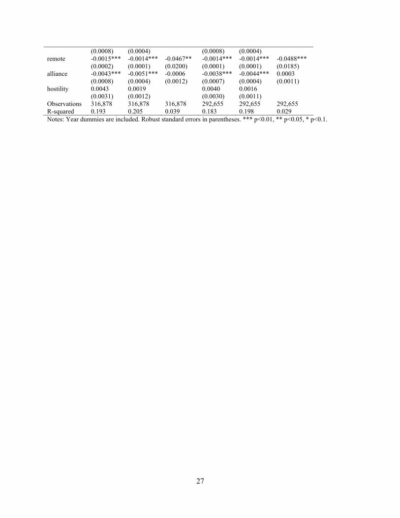
The results from regressions with spatial measures are reported in Table 3. The first three

columns use the current spatial measures, while the last three columns use lagged ones. Looking

tiV 1

13

across columns in Table 3, different specifications give qualitatively similar results. Coefficients

on measures of spatial volatilities are positive and significant at the 1% level in all regressions,

indicating a general synchronization of trade volatilities. The positive coefficient on the term Vi1t

shows that for dyad ij with both partners as WTO members, an increase in the volatility of

imports of i from other WTO exporters is associated with an increase in the volatility of import

in i from j. In other words, trade between WTO members i and j is more stable if trade between

the same country i and other WTO exporters m is more stable. Similarly, the positive coefficient

on V1jt implies that imports of WTO member country i from WTO member country j are more

stable if trade between other WTO importers and the same exporting country j is more stable.

These results suggest that for WTO members, there is a strong interdependence or comovement

of their trade volatilities with other WTO members.

The estimated coefficients on Vi0 t and V0 jt are also positive and significant at the 1%

level, implying a synchronization of trade volatilities between WTO members and non-WTO

members as well. However, the strength of the comovement of trade volatilities among WTO

members and the strength of the comovement between WTO and non-WTO members are

considerably different. The estimated coefficients on Vi1t and V1 jt range between 0.346-0.657

and between 0.285-0.612, respectively. In contrast, the estimated coefficients on Vi0 t and V0 jt

range between 0.037-0.069 and between 0.048-0.083, respectively. So the clustering of trade

volatilities between WTO members and non-WTO members is much weaker than that among

WTO members.

4.3 Robustness Checks

In this section, we provide a number of robustness checks to ensure an appropriate interpretation

of our results. We begin by adopting two alternative weight matrices to calculate spatial

volatilities. We first incorporate geographical distance in the weight matrix. To be specific, we

replace the weight wWTO in the contagion spatial term Vi1 by wWTO 1/ dist jm , with dist jm

representing the distance between countries j and m. An inverse distance weight is applied to

assign a larger weight to those dyads with exporters geographically closer to country j. For

example, this suggests we would expect the volatility of imports of Thailand (i) from the U.S. (j)

may be influenced more by the volatility of imports of Thailand from Canada (m) than the

14

volatility of imports of Thailand from the U.K. (m) as Canada is closer to the U.S. than the U.K.

Similarly, for the second importer contagion, Vi0, the weight wnonWTO is replaced by

wnonWTO 1/ dist jm . We also apply the same technique to generate the new weight in the two

exporter contagion terms: WTO 1/ distik and nonWTO 1/ distik . For the dyad ij of interest, a

larger weight is assigned to those pairs located closer to country i or j, holding WTO

membership constant. This larger weight would imply, for instance, the interdependence of

volatility of imports of Thailand (i) from the U.S. (j) and the volatility between the imports of

Malaysia (k) from the U.S. should be stronger than the interdependence between the import

volatility in Thailand from the U.S. and the import volatility of South Africa (k) from the U.S. as

Malaysia is closer to Thailand than South Africa.

The second alternative weight matrix measures the connectivity among countries based

on their “economic distance.” Countries can be geographically far apart while sharing a strong

economic bond and in turn experience a strong synchronization of trade volatilities (Clark and

van Wincoop, 2001; Baxter and Kouparitsas, 2005). Countries are considered economically

closer if they conduct a large volume of trade with each other, ceteris paribus. In particular, we

replace 1/ dist jm in the spatial weight by tradejm to construct the new importer specific contagion

terms, and 1 / distik by tradeik for new exporter specific contagion terms, where tradejm is the

log value of total trade between countries j and m, and tradeik the log value of total trade

between countries i and k. Hence, the weights in exporter specific contagion terms become

wWTO tradejm and wnonWTO tradejm , and the weights in importer specific contagion terms

become WTO tradeik and nonWTO tradeik .

In addition, we estimate regressions without the U.S., the world leading economy, to

make sure that the comovement of trade volatilities is not driven simply by a dominant country.

The OPEC countries are also excluded from the sample to alleviate influences from global oil

supply shocks. To eliminate these countries completely, we drop them not only from our final

data sample for regressions, but also from the data we use to reconstruct the spatial lag measures.

Results including distance- and trade-weighted spatial volatility measures are provided in

panel (A) in Table 4. Results for subsamples excluding the U.S. or the OPEC countries are

presented in panel (B) in Table 4. For the purpose of brevity, we only report estimated

15

coefficients on contemporaneous importer and exporter specific contagions and the estimated

coefficients on RTA, GSP, and CU. Other results, including regressions with lagged spatial

volatilities, are available upon request.

As we can see, results in Table 4 are in general consistent with results in Table 3.

Estimated coefficients on all spatial lag terms are positive and significant. Panel (A) suggests

clustering of trade volatilities among geographical neighbors and among those who have strong

economic ties with each other. This is especially true for WTO members as the coefficients on

WTO specific exporter and specific importer contagion terms are significantly larger than the

coefficients on non-WTO specific exporter and specific importer contagion terms. Panel (B)

indicates that our findings are robust to different subsamples with or without the U.S. or the

OPEC countries.

Next, we conduct additional robustness checks with alternative measures of trade

volatilities and report results from 18 regressions in Table 5. Again, to save space, we only

present the coefficients on spatial measures with other results available upon request. Three

alternative measures of trade volatilities are used for Table 5 regressions. We start with the

volatility measure used in Rose (2005), which is the coefficient of variation of imports:8

Vol Mij T Mijt

T

Mijt T (8)

where Mijt T

is the standard deviation of imports of country i from j over a time period T, and

Mijt T

denotes the mean value of imports over the same period. We construct the other two

alternative measures based on popular methods used to construct macroeconomic volatilities.

Our second measure of trade volatility for robustness checks is the standard deviation of the

difference between actual and Hodrick-Prescott (HP) filtered imports as represented in equation

(9) below:

Vol Mij T

eijt2

T 1 (9)

8 Rose (2005) uses exports from i to j to construct the volatility measure.

16

where eijt Mijt MijtHP is the difference between actual imports of i from j and the HP-filtered

series ( ).9 The third alternative measure of trade volatility is the standard deviation of

imports growth in country i from country j over a certain period (Bullard, 1998), shown as

follows:

Vol Mij T

gijt gijt / T 2

T 1

(10)

where gijt is the growth of imports of i from j in year t.

Since the volatilities in equations (8)-(10) are measured by standard deviations, we will

have one observation for each dyad over a certain time period T. As a result, control variables in

the regressions for Table 6 are all averaged over the same time period T. We run three sets of

regressions, changing number of years included in a period T. To be more specific, the first set of

regressions cover pre- and post-Uruguay rounds of GATT (T1=1948-1985 and T2=1986-2003).

Following Kose et al. (2008), the second set of regressions cover the post WWII and Breton

Woods era of 1948-1972 (T1), the common international shock period of 1973-1986 (T2), and the

globalization era of 1987-2003 (T3). The last set of regressions cover different stages of

GATT/WTO: pre-Kennedy round of 1948-1967 (T1), Kennedy to Tokyo round of 1968-1978

(T2), Tokyo to Uruguay round of 1979-1994 (T3), and post Uruguay round (WTO) of 1995-2003

(T4) (Felbermayr and Kohler, 2010).10

Table 5 in general presents a similar picture as previous tables with respect to qualitative

results concerning trade volatilities among WTO members. The estimated coefficients on

exporter and importer specific contagion terms based on WTO membership are positive and

significant in all regressions. Interestingly, non-WTO exporter contagion terms are negative in

9 The Hodrick-Prescott (HP) filter is a filter for trend and business cycle estimation. Assume a variable yt can be decomposed into a trend and a business cycle component. The HP filter finds a trend estimate by solving a penalized optimization problem. The business cycle component is the difference between actual yt and the HP filter trend estimate. 10 Regressions in Table 5 are estimated using instrumental variables (IV) estimation to control for potential endogeneity of the spatial terms, which is typically used in the literature. Following Kelejian et al. (2004), instruments for spatial volatilities are WX and WWX, where W is the WTO weight matrix used to create the exporter and importer specific contagion terms in Table 3, and X is the vector of control variables used in our regressions. The number of observations in Table 5 regressions is about one tenth or one fifth of the number of observations in previous tables. Constructing the instruments WX and WWX for regressions in Table 5 is computational intensive but still feasible. In previous regressions with 60 years of data, however, calculating WX and WWX is computationally unfeasible.

17

13 out of 18 regressions and are statistically significant in 10 regressions. Non-WTO importer

specific contagion terms are negative in 14 regressions and statistically significant in six of them.

Table 5 seems to present even stronger results than Tables 3 and 4. The results support

synchronization of trade volatilities among WTO member trade partners. In contrast, volatility of

trade between WTO members either is not strongly correlated with or diverges from the trade

volatility between WTO and non-WTO members.

Finally, time-varying country fixed effects (TVCFEs) can be used in a gravity regression

to capture the “multilateral resistance”.11 However, Vi0 and V0j will be dropped when TVCFEs

are included, so we can no longer see the different effects of the spatial lags based on countries’

WTO membership. This is also why we choose to use the measure of remoteness for multilateral

resistance.12 Without TVCFEs, we might observe a spurious correlation between our dependent

variable and our spatial trade volatility terms. However, the spurious correlation alone could not

explain why the coefficients on Vi1 and V1j are much larger than those on Vi0 and V0j. In other

words, WTO membership must play a role.

5. How to Cope with Contagion?

If countries under the WTO share the risk of trade volatility, one natural question is what we can

do to alleviate this problem. Are there specific policy instruments countries can use to cope with

contagion? In this paper, we examine specifically whether some country or dyad characteristics,

such as country size and policies related to signing other types of integration agreements, can

help in this regard. To answer this question, we add to our baseline regressions some interaction

terms between the spatial lag measures and country’s GDP and indicators for RTAs, CUs, and

GSP. Our results in the previous section show a statistically and economically similar effect of 11 In bilateral trade analysis, to obtain consistent results, a measure reflecting trade frictions between a specific country pair and all other trade partners in addition to trade frictions between i and j needs to be included, addressed as the “multilateral resistance effect” in Anderson and van Wincoop (2003). As discussed in the literature, however, accounting for the multilateral resistance term is challenging. For example, Hummels (2007) use country-fixed effects for importers and exporters to control for the multilateral resistance while Baldwin and Taglioni (2006) point out that those fixed effects should be time-varying. As we have a large sample covering 210 countries over the period 1948-2003, time-varying country fixed effects could be computationally impractical. 12 As previously mentioned, including time-varying country fixed effects may be computationally impractical in our study. In addition, the variations in in Vi1 and V1j measures may be small in later years when there are many WTO members. Not much information will be left once TVCFEs are included and the coefficients of Vi1 and V1j may not be estimated precisely. We recognize that without including time-varying country dummies, our results may be driven by country-year specific unobserved heterogeneity. For example, an economic boom in country i could lead to higher trade with all trading partners, and in turn a positive association between Vol(Mij) and the spatial lag terms. Including ln(GDP) can help to control for economic booms or recessions and alleviate such a concern.

18

Vi1 and V1j, and of Vi0 and V0j. To avoid adding too many interaction terms and ease the

interpretation, we combine Vi1 and V1j into one term named V1, and also combine Vi0 and V0j into

one term named V0. For a similar reason, we also combine log value of GDP for the two

countries in a dyad into lgdpsum, defined as the sum of ln GDPi and ln GDPj in a dyad. The

results are reported in Table 6.

First, the negative coefficients of V1*lgdpsum and V0*lgdpsum suggest that larger

economic size can help to alleviate the contagion, especially the contagion within the WTO. This

is not surprising because larger countries, which usually rely more on domestic markets, are

more resilient to external risks. The weaker effect of V0*lgdpsum than that of V1*lgdpsum may

result from the much smaller level effect of V0 (i.e., the smaller coefficient on V0 as compared to

the coefficient of V1). RTAs and CUs between two WTO members also help to alleviate the

contagion within the WTO as suggested by the negative and significant coefficients of V1*RTA

and V1*CU. Their effects on the contagion from outside the WTO are much weaker as shown by

the insignificant and much smaller coefficients of V0*RTA and V0*CU, which can also be

partially driven by the much smaller level effect of V0. But this is unlikely the only reason

because estimated coefficients on V1*GSP and V0*GSP are both negative and significant, with a

similar magnitude. Another possible interpretation is that, in our restricted sample with both

countries in a dyad being WTO members, V0 is based on the trade between WTO members and

non-WTO members which usually constitutes a small portion of the trade of WTO members,

while trade within the WTO and covered by RTAs or CUs are usually among major or natural

trading partners. In other words, the trade flows related to V0 and those related to RTAs/CUs are

not very relevant to each other, which may explain the insignificant interaction effect between

RTAs (CUs) and V0.

Overall, results in Table 6 point out a benign role of other types of trade and common

currency agreements that can help a country to diversify its trade, and hence make it less

vulnerable to external trade volatility. However, a country can only alleviate the contagion

problem to some extent. This problem cannot be completely eliminated as suggested by the

smaller coefficients of the interaction terms relative to the much larger coefficient of V1, with the

only exception of V0*GSP. This is true even for U.S.-China, the country pair with the largest

combined GDP in logarithms in our sample at a value of 31.56 in 2002. Taking the third

regression in Table 6 as an example, the overall effect of V1 is still positive for U.S.-China in

19

2002 (i.e., 1.287-0.038*33.56 = 0.012). The corresponding estimated effect of V1 for a dyad with

an average combined ln(GDP) at a value of 21.49, our sample average, is 0.47, ceteris paribus.

6. Conclusions

Several studies have suggested that exposure to global markets increases terms of trade volatility

and governments try to insulate their economies from such instability through membership in

international trade institutions like the WTO and preferential trading arrangements. Research

exploring the relationship between WTO and trade volatility is rather scarce, and the existing

studies on this topic do not focus on the interdependence of trade volatilities across dyads. In

fact, it is possible that bilateral trade volatility is affected by trade volatility between other dyads.

Omitting such a measure of the interdependence of trade volatility can lead to biased estimates

and invalid statistical inferences.

Using bilateral trade data for 210 countries over the period 1948-2003, this paper

attempts to shed some light on the WTO and its members’ trade volatilities by concentrating on

three questions: (i) does the GATT/WTO reduce the bilateral trade volatility? (ii) how does the

bilateral trade volatility of WTO members co-vary with the volatilities of their trading partners,

depending on partners’ WTO membership? and (iii) how countries can cope with the contagion?

The initial results suggest that if both trade partners are de facto WTO members, they

tend to experience more stable trade. After controlling for spatial trade volatilities, we find that

trade volatilities commove among different dyads. Such a comovement is more evident between

two dyads within the WTO than between a dyad within the WTO and another dyad with at least

one country outside the WTO. RTAs, GSP, and currency unions not only contribute to more

stable trade of a dyad, but also help to alleviate the contagion by diversifying a country’s trade

risks and reducing trade volatility. A large economic size is also found to be able to help a

country cope with the contagion.

Recent empirical research about the impact of international trade organizations highlights

the increase in the level of trade without taking trade volatility into account. Once that is done,

the beneficial impact of trade organizations and trade agreements becomes clearer.

For policy purposes, it is important to note that the comovement of trade volatilities

among WTO members implies that member countries share the benefits of having an

interdependent and more predictable trade system. However, they also share the risks of

20

contagious world trade crisis. Nevertheless, a better understanding of this interdependence can

enhance our awareness so that countries are more cautious when implementing policies that

might affect adversely other countries and are more prepared to cope with these risks. Our results

indicate that signing other types of integration agreements can help in this regard.

References

Aizenman, J., 2003. “Volatility, Employment, and the Patterns of FDI in Emerging Markets.” Journal of Development Economics 72(2): 585-601. Bagwell, K., and R.W. Staiger, 2002. The Economics of the World Trading System. MIT Press, Cambridge, Massachusetts and London, England. Baier, S.L., and J.H. Bergstrand, 2007. “Do Free Trade Agreements Actually Increase

Members’International Trade?” Journal of International Economics 71(1): 72‐95.

Balding, C., 2010. “Joining the World Trade Organization: What is the Impact?” Review of

International Economics 18(1): 193‐206.

Baldwin, R., and D. Taglioni, 2006. "Gravity for Dummies and Dummies for Gravity Equations." NBER Working Papers 12516. Baxter, M., and M. Kouparitsas, 2005. “Determinants of Business Cycle Comovement: A Robust Analysis.” Journal of Monetary Economics 52(1): 113-157. Bhagwati, J., 1991. The World Trading System at Risk. Princeton, N.J.: Princeton University Press. Blattman, C., J. Hwang, and J. Williamson. 2007. “Winners and Losers in the Commodity Lottery: The Impact of Terms of Trade Growth and Volatility in the Periphery 1870-1939.” Journal of Development Economics 82(1): 152-179. Braumoeller, B., 2006. “Explaining Variance: Or, Stuck in a Moment We Can’t Get Out Of.” Political Analysis 14: 268–290. Bullard, J. 1998. “Trading Trade-Offs?” National Economic Trends. St. Louis: Federal Reserve Bank of St. Louis. December. Clark, T., and E. van Wincoop, 2001. “Borders and Business Cycles.” Journal of International Economics 55(1): 59-85.

21

Egger, P., and M. Larch,2008. “Interdependent preferential trade agreement member-ships: An empirical analysis.” Journal of International Economics 76: 384–399. Felbermayr, G., and W. Kohler, 2010. "Modelling the ExtensiveMargin ofWorldTrade:NewEvidenceonGATTandWTOMembership." TheWorldEconomy 33(11): 1430-1469. Grimes, A., 2006. “A Smooth Ride: Terms of Trade, Volatility and GDP growth.” Journal of Asian Economics 17(4): 583–600. Haddad, M., J. Lim, C. Pancaro, and C. Saborowski, 2012. “Trade Openness Reduces Growth Volatility When Countries are Well Diversified.” European Central Bank Working Paper Series No. 1491, November. Helpman, E., M. Melitz, and Y. Rubinstein, 2008. “Estimating trade Flows: Trading Partners and

Trading Volumes.” Quarterly Journal of Economics 123(2): 441‐487.

Hidalgo, D., S. Naidu, S. Nichter, and N. Richardson, 2010. “Economic Determinants of Land Invasions.” The Review of Economics and Statistics 92(3): 505–523. Hummels, D., 2007. “Transportation costs and international trade in the second era of globalization.” Journal of Economic Perspective 21(3): 131–154. Kellman, M., and Y. Shachmurove, 2011. “Diversification and Specialization paradox in Developing Country Trade.” Review of Development Economics 15(2): 212-222. Kim, S.Y., 2007. “Openness, External Risk, and Volatility: Implications for the Compensation Hypothesis.” International Organization 62(3):477–505. Kose, M.A., C. Otrok and C.H. Whiteman, 2008. “Understanding the Evolution of World Business Cycles.” Journal of International Economics 75 (1): 110–130. Liu, X., 2009. “GATT/WTO Promotes Trade Strongly: Sample Selection and Model Specification.” Review of International Economics 17(3): 428‐446. Mansfield, E., and E. Reinhardt, 2008. “International Institutions and the Volatility of International Trade.” International Organization 62(4): 621-652. Marting, L., and B. Simmons. 1998. “Theories and Empirical Studies of International Institutions.” International Organization 52(4): 729-757.

22

Miguel, E., S. Satyanath, and E. Sergenti, 2008. “Economic Shocks and Civil Conflict: An Instrumental Variables Approach.” Journal of Political Economy 112(4): 725-753. Neumayer, E., and P. Thomas, 2010. “Spatial effects in dyadic data.” International organization 64 (1): 145-166. Nielsen, R., M. Findley, Z. Davis, T. Candland, and D.. Nielson, 2011. “Foreign Aid Shocks as a Cause of Violent Armed Conflict.” American Journal of Political Science 55(2): 219-232. Razin, A., E. Sadka, and T. Coury, 2003. “Trade Openness, Investment Instability and Terms-of-Trade Volatility.” Journal of International Economics 61(2): 285–306. Rodrik, D., 1998. “Why Do More Open Economies Have Bigger Governments.” Journal of Political Economy 106(5): 997–1032. Rodrik, D., 1999. “Where Did All the Growth Go? External Shocks, Social Conflict, and Growth Collapses.” Journal of Economic Growth 4(4): 385–412. Rose, A., 2004. “Do We Really Know That the WTO Increases Trade?” American Economic

Review 94(1): 8‐114.

Rose, A., 2005. “Does the WTO Make Trade More Stable?” Open Economies Review 16(1): 7-22. Scheve, K. and M. Slaughter, 2004. “Economic Insecurity and the Globalization of Production.” American Journal of Political Science 48(4): 662-674. Subramanian A. and S.J. Wei. 2007, “The WTO Promotes Trade Strongly but Unevenly.”

Journal of International Economics 72(1): 151‐175.

Tobler, W., 1970. “A Computer Movie Simulating Urban Growth in the Detroit Region.” Economic Geography 46(2): 234-240. Tomz, M., J. Goldstein, and D. Rivers, 2007. “Do We Really Know that the WTO Increases Trade? Comment.” American Economic Review 97(5): 2005‐2018. WTO, 2007. World Trade Report 2007. Six Decades of Multilateral Trade Cooperation: What have we Learnt? WTO Document WT/REG/E/37, March.

23

Figure 1: Spatial measures for dyad ij, with arrows denoting the directions of trade

24

Table 1. Descriptive statistics Variables Mean Standard Deviation Minimum Maximum Observations

Vol(Mijt) 0.0441 0.0584 0 3.0229 556182

Bothin 0.6185 0.4858 0 1 556182

Vi1t 0.0392 0.0184 0.0001 0.2787 555896

Vi0t 0.0541 0.0274 2.53E-05 0.4008 552665

V1jt 0.0416 0.0227 1.35E-05 0.2751 555797

V0jt 0.0479 0.0278 1.39E-05 0.7776 550541

RTA 0.1083 0.3107 0 1 556182

GSP 0.1610 0.3676 0 1 556182

CU 0.0311 0.1737 0 1 556182

ln(GDPi) 10.5362 2.1580 0.8154 16.0953 533895

ln(GDPj) 10.9315 1.9988 0.8154 16.0953 536734

ln(GDPPCi) 1.6076 1.0767 -1.9700 3.9010 533895

ln(GDPPCj) 1.6667 1.0482 -1.9700 3.9010 536734

ln(AREAi) 11.8180 2.5502 1.9459 16.9247 556182

ln(AREAj) 12.1019 2.4111 1.9459 16.9246 556182

border 0.0339 0.1811 0 1 556182

landlock 0.2612 0.4805 0 2 556182

island 0.3580 0.5583 0 2 556182

samelang 0.1255 0.3313 0 1 556182

samerelig 0.5620 0.4961 0 1 556182

colony 0.0137 0.1161 0 1 556182

colonizer 0.0131 0.1135 0 1 556182

curcolony 0.0026 0.0507 0 1 556182

curcolonizer 0.0024 0.0493 0 1 556182

comcol 0.1568 0.3636 0 1 556182

remote 0.9374 1.7841 0 4.5095 556182

alliance 0.1016 0.3022 0 1 556182

hostility 0.0176 0.1100 0 2.5179 556182

Note: See Section 3.1 for the definitions of these variables.

25

Table 2. Results of WTO membership and trade volatility 2.1 2.2 2.3 VARIABLES OLS Ctry FE Dyad FE Bothin -0.0033*** -0.0054*** -0.0051*** (0.0004) (0.0003) (0.0004) RTA -0.0041*** -0.0070*** -0.0052*** (0.0006) (0.0003) (0.0006) GSP -0.0109*** -0.0093*** -0.0041*** (0.0005) (0.0003) (0.0005) CU -0.0064*** -0.0072*** -0.0100*** (0.0015) (0.0006) (0.0024) ln(GDPi) -0.0044*** -0.0002 -0.0047*** (0.0002) (0.0005) (0.0009) ln(GDPj) -0.0089*** -0.0058*** -0.0038*** (0.0002) (0.0005) (0.0010) ln(GDPPCi) -0.0060*** -0.0083*** -0.0042*** (0.0003) (0.0004) (0.0009) ln(GDPPCj) -0.0014*** -0.0078*** -0.0088*** (0.0003) (0.0005) (0.0011) ln(AREAi) 0.0015*** 0.0024*** (0.0001) (0.0007) ln(AREAj) 0.0030*** (0.0001) border -0.0104*** -0.0089*** (0.0012) (0.0004) landlock -0.0034*** 0.0131*** (0.0004) (0.0032) island 0.0026*** 0.0769*** (0.0004) (0.0083) samelang -0.0018** -0.0058*** (0.0009) (0.0004) samerelig -0.0014*** -0.0024*** (0.0004) (0.0002) colony -0.0097*** -0.0086*** (0.0012) (0.0004) colonizer -0.0178*** -0.0114*** (0.0017) (0.0005) curcolony -0.0040 0.0012 0.0045** (0.0025) (0.0008) (0.0019) curcolonizer -0.0011 -0.0027** 0.0077** (0.0037) (0.0012) (0.0032) comcol -0.0029*** -0.0045*** (0.0008) (0.0003) remote -0.0017*** -0.0013*** -0.0290* (0.0001) (0.0001) (0.0173) alliance -0.0035*** -0.0043*** 0.0016* (0.0007) (0.0003) (0.0009) hostility 0.0074*** 0.0015** (0.0019) (0.0007) Observations 521,852 521,852 521,852 R-squared 0.121 0.171 0.017 Notes: Year dummies are included. Robust standard errors in parentheses. *** p<0.01, ** p<0.05, * p<0.1.

26

Table 3. Results with spatial dyadic trade volatility for WTO countries 3.1 3.2 3.3 3.4 3.5 3.6

VARIABLES OLS Ctry FE Dyad FE OLS lag Ctry FE lag Dyad FE lag Vi1t 0.6572*** 0.5199*** 0.4996*** (0.0154) (0.0116) (0.0139) Vi0t 0.0694*** 0.0846*** 0.0541*** (0.0085) (0.0064) (0.0070) V1jt 0.6122*** 0.3800*** 0.4141*** (0.0175) (0.0128) (0.0165) Vj0t 0.0831*** 0.0684*** 0.0624*** (0.0079) (0.0066) (0.0068) Vi1,t-1 0.5469*** 0.3821*** 0.3485*** (0.0148) (0.0112) (0.0130) Vi0,t-1 0.0675*** 0.0751*** 0.0372*** (0.0082) (0.0061) (0.0066) V1j,t-1 0.5452*** 0.2848*** 0.2997*** (0.0171) (0.0126) (0.0161) Vj0,t-1 0.0802*** 0.0588*** 0.0482*** (0.0079) (0.0070) (0.0068) RTA -0.0042*** -0.0051*** -0.0043*** -0.0035*** -0.0046*** -0.0042*** (0.0007) (0.0003) (0.0007) (0.0006) (0.0003) (0.0006) GSP -0.0077*** -0.0108*** -0.0041*** -0.0064*** -0.0094*** -0.0030*** (0.0006) (0.0003) (0.0006) (0.0006) (0.0003) (0.0005) CU -0.0066*** -0.0064*** -0.0063** -0.0059*** -0.0059*** -0.0062** (0.0016) (0.0006) (0.0027) (0.0015) (0.0006) (0.0026) ln(GDPi) -0.0029*** 0.0027*** -0.0027** -0.0029*** 0.0017*** -0.0052*** (0.0002) (0.0006) (0.0011) (0.0002) (0.0006) (0.0011) ln(GDPj) -0.0039*** -0.0063*** -0.0040*** -0.0040*** -0.0064*** -0.0056*** (0.0002) (0.0007) (0.0014) (0.0002) (0.0007) (0.0014) ln(GDPPCi) -0.0028*** -0.0078*** -0.0026** -0.0027*** -0.0066*** -0.0002 (0.0003) (0.0006) (0.0010) (0.0003) (0.0006) (0.0010) ln(GDPPCj) -0.0002 -0.0015** -0.0024* -0.0003 -0.0018** -0.0007 (0.0003) (0.0008) (0.0015) (0.0003) (0.0008) (0.0014) ln(AREAi) 0.0008*** -0.0044*** 0.0008*** -0.0043*** (0.0001) (0.0007) (0.0001) (0.0008) ln(AREAj) 0.0013*** 0.0013*** (0.0001) (0.0001) border -0.0068*** -0.0063*** -0.0061*** -0.0056*** (0.0016) (0.0006) (0.0015) (0.0006) landlock -0.0008 -0.0121*** -0.0006 -0.0020 (0.0005) (0.0046) (0.0005) (0.0047) island 0.0015*** 0.0047** 0.0014*** 0.0054** (0.0005) (0.0022) (0.0005) (0.0022) samelang -0.0030*** -0.0056*** -0.0034*** -0.0060*** (0.0010) (0.0005) (0.0010) (0.0004) samerelig -0.0018*** -0.0025*** -0.0016*** -0.0021*** (0.0005) (0.0003) (0.0005) (0.0003) colony -0.0073*** -0.0083*** -0.0067*** -0.0076*** (0.0014) (0.0005) (0.0013) (0.0005) colonizer -0.0150*** -0.0136*** -0.0142*** -0.0125*** (0.0016) (0.0006) (0.0016) (0.0006) curcolony 0.0008 0.0025*** 0.0031 0.0002 0.0018** 0.0019 (0.0020) (0.0008) (0.0019) (0.0019) (0.0008) (0.0019) curcolonizer 0.0045 0.0002 0.0114*** 0.0041 -0.0012 0.0094*** (0.0034) (0.0013) (0.0032) (0.0029) (0.0013) (0.0028) comcol -0.0046*** -0.0052*** -0.0043*** -0.0045***

27

(0.0008) (0.0004) (0.0008) (0.0004) remote -0.0015*** -0.0014*** -0.0467** -0.0014*** -0.0014*** -0.0488*** (0.0002) (0.0001) (0.0200) (0.0001) (0.0001) (0.0185) alliance -0.0043*** -0.0051*** -0.0006 -0.0038*** -0.0044*** 0.0003 (0.0008) (0.0004) (0.0012) (0.0007) (0.0004) (0.0011) hostility 0.0043 0.0019 0.0040 0.0016 (0.0031) (0.0012) (0.0030) (0.0011) Observations 316,878 316,878 316,878 292,655 292,655 292,655 R-squared 0.193 0.205 0.039 0.183 0.198 0.029 Notes: Year dummies are included. Robust standard errors in parentheses. *** p<0.01, ** p<0.05, * p<0.1.

28

Table 4. Robustness checks, WTO sample (A). Alternative weights for spatial lags

WTO and distance weight for spatial lags WTO and trade weight for spatial lags 4.A.1 4.A.2 4.A.3 4.A.4 4.A.5 4.A.6

Variables OLS Ctry FE Dyad FE OLS Ctry FE Dyad FE Vi1t 0.455*** 0.424*** 0.341*** 0.541*** 0.414*** 0.433*** (0.013) (0.010) (0.012) (0.018) (0.017) (0.016) Vi0t 0.053*** 0.047*** 0.033*** 0.041*** 0.030*** 0.022*** (0.005) (0.004) (0.005) (0.006) (0.006) (0.005) V1jt 0.570*** 0.464*** 0.332*** 0.682*** 0.412*** 0.395*** (0.014) (0.010) (0.013) (0.021) (0.020) (0.019) Vj0t 0.049*** 0.046*** 0.036*** 0.039*** 0.038*** 0.025*** (0.005) (0.004) (0.004) (0.006) (0.005) (0.005) RTA -0.002*** -0.004*** -0.004*** -0.003*** -0.004*** -0.004*** (0.001) (0.000) (0.001) (0.001) (0.001) (0.001) GSP -0.006*** -0.008*** -0.003*** -0.009*** -0.010*** -0.003*** (0.001) (0.000) (0.001) (0.001) (0.001) (0.001) CU -0.005*** -0.004*** -0.005* -0.005*** -0.004** -0.005 (0.002) (0.001) (0.003) (0.002) (0.002) (0.003) Observations 288,951 288,951 288,951 227,580 192,962 227,580 R-squared 0.211 0.227 0.038 0.198 0.218 0.033

(B) Without the U.S. or the OPEC countries

Excluding the U.S. Excluding OPEC Countries 4.B.1 4.B.2 4.B.3 4.B.4 4.B.5 4.B.6 Variables OLS Ctry FE Dyad FE OLS Ctry FE Dyad FE Vi1t 0.6240*** 0.5145*** 0.4928*** 0.628*** 0.499*** 0.476*** (0.0151) (0.0145) (0.0141) (0.0158) (0.0123) (0.0147) Vi0t 0.0637*** 0.0705*** 0.0425*** 0.0515*** 0.0604*** 0.0342*** (0.0077) (0.0066) (0.0062) (0.00753) (0.00595) (0.00614) V1jt 0.6661*** 0.4075*** 0.4519*** 0.642*** 0.388*** 0.436*** (0.0188) (0.0181) (0.0177) (0.0193) (0.0147) (0.0184) Vj0t 0.0482*** 0.0517*** 0.0434*** 0.0452*** 0.0446*** 0.0379*** (0.0064) (0.0057) (0.0055) (0.00639) (0.00561) (0.00561) RTA -0.0037*** -0.0047*** -0.0042*** -0.0045*** -0.0054*** -0.0041*** (0.0007) (0.0007) (0.0007) (0.00069) (0.00036) (0.00071) GSP -0.0072*** -0.0104*** -0.0035*** -0.0077*** -0.0111*** -0.0032*** (0.0006) (0.0007) (0.0006) (0.00062) (0.00035) (0.00059) CU -0.0061*** -0.0056*** -0.0065** -0.0072*** -0.0069*** -0.0077*** (0.0017) (0.0017) (0.0028) (0.00160) (0.000697) (0.00297) Observations 299,497 299,497 299,497 282,161 282,161 282,161 R-squared 0.189 0.202 0.039 0.194 0.208 0.036

Notes: Year dummies are included. Robust standard errors in parentheses. *** p<0.01, ** p<0.05, * p<0.1.

29

Table 5. Robustness checks with alternative measures of trade volatilities, WTO Sample Rose (2005) Measure Import Growth Measure HP-filter Measure

SUBSAMPLES VARIABLES Ctry FE Dyad FE Ctry FE Dyad FE Ctry FE Dyad FE Pre-Kennedy round of 1948-196, Kennedy to Tokyo round of 1968-1978, Tokyo to Uruguay round of 1979-1994, and post Uruguay round (WTO) of 1995-2003.

Vi1t 0.86148** 0.91336*** 0.85096*** 0.80429*** 1.11073*** 1.12253*** (0.102) (0.080) (0.084) (0.068) (0.090) (0.079)

Vi0t -0.18581*** -0.30039*** -0.16530*** -0.22932*** -0.34989*** -0.38081*** (0.062) (0.050) (0.054) (0.044) (0.067) (0.060)

V1jt 0.95311*** 0.77529*** 0.86710*** 0.63564*** 1.09687*** 1.12880*** (0.093) (0.075) (0.091) (0.075) (0.082) (0.073)

Vj0t 0.00709 0.08364 0.02967 0.15814** -0.10059 -0.09426 (0.085) (0.069) (0.082) (0.067) (0.074) (0.066)

Observations 24,136 24,136 23,079 23,079 25,001 25,001 R-squared 0.3402 0.3432 0.3568 0.3289 0.3021 0.3113

Post WWII and Breton Woods era of 1948-1972, the common international shock period of 1973-1986, and the globalization era of 1987-2003.

Vi1t 0.57269*** 0.85792*** 0.47904*** 0.60978*** 1.18510*** 1.22754*** (0.126) (0.100) (0.120) (0.096) (0.098) (0.090)

Vi0t -0.02273 -0.25016*** 0.04523 -0.07349 -0.39090*** -0.44855*** (0.081) (0.064) (0.083) (0.065) (0.075) (0.069)

V1jt 0.94924*** 0.89642*** 0.98638*** 0.80067*** 1.20489*** 1.20076*** (0.096) (0.078) (0.095) (0.080) (0.091) (0.086)

Vj0t -0.17952* -0.17138** -0.11741 -0.04147 -0.29481*** -0.30010*** (0.097) (0.078) (0.090) (0.076) (0.091) (0.086)

Observations 15,756 15,756 15,128 15,128 16,259 16,259R-squared 0.3921 0.3936 0.3928 0.3812 0.3216 0.3324

Pre- and post-Uruguay rounds of GATT (1948-1985, 1986-2003)

Vi1t 0.67207*** 0.97739*** 0.91554*** 0.79179*** 1.65789*** 0.29509*** (0.189) (0.209) (0.200) (0.212) (0.169) (0.187)

Vi0t 0.06504 -0.02695 0.07285 0.1976 -0.61584*** -0.18502 (0.117) (0.125) (0.139) (0.145) (0.135) (0.146)

V1jt 0.80723*** 0.98688*** 0.84042*** 0.84266*** 1.69377*** 1.19779*** (0.152) (0.161) (0.140) (0.153) (0.178) (0.189)

Vj0t 0.10793 -0.12676 -0.13473 -0.11773 -0.64828*** -0.22299 (0.140) (0.148) (0.137) (0.142) (0.174) (0.185

Observations 11,209 11,209 10,733 10,733 11,414 11,414 R-squared 0.3684 0.3567 0.3791 0.3449 0.3071 0.311

Notes: Robust standard errors in parentheses. *** p<0.01, ** p<0.05, * p<0.1.

30

Table 6: Interactions between spatial lags and dyadic characteristics Weighted by

WTO membershipWeighted by

WTO membership & distance Weighted by

WTO membership & trade 6.1 6.2 6.3 6.4 6.5 6.6 6.7 6.8 6.9 OLS Ctry FE Dyad FE OLS Ctry FE Dyad FE OLS Ctry FE Dyad FE V1 1.436*** 1.478*** 1.287*** 1.422*** 1.460*** 1.279*** 1.403*** 1.476*** 1.221*** (0.082) (0.051) (0.075) (0.081) (0.050) (0.075) (0.093) (0.057) (0.083) V1*RTA -0.154*** -0.180*** -0.041* -0.167*** -0.189*** -0.048** -0.151*** -0.185*** -0.024 (0.025) (0.016) (0.022) (0.025) (0.016) (0.022) (0.029) (0.019) (0.025) V1*CU -0.177*** -0.148*** -0.086** -0.183*** -0.158*** -0.086** -0.209*** -0.171*** -0.102** (0.044) (0.027) (0.041) (0.044) (0.026) (0.041) (0.048) (0.029) (0.045) V1*GSP -0.090*** -0.057*** -0.084*** -0.085*** -0.050*** -0.079*** -0.090*** -0.046*** -0.084*** (0.023) (0.014) (0.020) (0.023) (0.014) (0.019) (0.026) (0.016) (0.022) V1*lgdpsum -0.035*** -0.047*** -0.038*** -0.035*** -0.046*** -0.038*** -0.028*** -0.043*** -0.030*** (0.004) (0.002) (0.003) (0.004) (0.002) (0.003) (0.004) (0.003) (0.004) V0 0.139*** 0.170*** 0.091*** 0.140*** 0.176*** 0.091*** 0.138*** 0.165*** 0.081** (0.039) (0.030) (0.030) (0.039) (0.030) (0.030) (0.042) (0.033) (0.033) V0*RTA 0.009 0.009 0.003 0.014 0.012 0.005 0.006 0.006 0.007 (0.013) (0.010) (0.011) (0.013) (0.010) (0.011) (0.014) (0.011) (0.012) V0*CU -0.006 0.000 0.023 -0.005 0.002 0.022 -0.010 -0.003 0.024 (0.022) (0.016) (0.018) (0.022) (0.016) (0.018) (0.023) (0.017) (0.019) V0*GSP -0.126*** -0.108*** -0.045*** -0.125*** -0.109*** -0.045*** -0.130*** -0.114*** -0.044*** (0.011) (0.008) (0.008) (0.011) (0.008) (0.008) (0.012) (0.009) (0.009) V0*lgdpsum -0.003* -0.005*** -0.002 -0.003* -0.005*** -0.002 -0.003 -0.004*** -0.002 (0.002) (0.001) (0.001) (0.002) (0.001) (0.001) (0.002) (0.002) (0.002) RTA 0.010*** 0.012*** -0.000 0.011*** 0.012*** 0.000 0.008*** 0.010*** -0.003 (0.002) (0.001) (0.002) (0.002) (0.001) (0.002) (0.002) (0.001) (0.002) CU 0.011*** 0.008*** -0.001 0.012*** 0.009*** -0.001 0.013*** 0.009*** -0.001 (0.003) (0.002) (0.004) (0.003) (0.002) (0.004) (0.003) (0.002) (0.004) GSP 0.013*** 0.008*** 0.008*** 0.013*** 0.008*** 0.008*** 0.011*** 0.006*** 0.007*** (0.002) (0.001) (0.001) (0.002) (0.001) (0.001) (0.002) (0.001) (0.001) lgdpsum -0.000 0.004*** -0.000 -0.000 0.004*** -0.000 -0.001*** 0.004*** -0.000 (0.000) (0.001) (0.001) (0.000) (0.001) (0.001) (0.000) (0.001) (0.001) Observations 309,874 309,874 309,874 309,874 309,874 309,874 309,874 309,874 309,874 R-squared 0.198 0.211 0.041 0.198 0.211 0.041 0.197 0.209 0.040 Notes: Year dummies are always included. Robust standard errors in parentheses. *** p<0.01, ** p<0.05, * p<0.1.