Job Shop Scheduling

Job Shop

A work location in which a number of general purpose work stations exist and are used to perform a variety of jobsExample: Car repair – each operator (mechanic) evaluates plus schedules, gets material, etc. – Traditional machine shop, with similar machine types located together, batch or individual production

Factors to Describe Job Shop Scheduling Problem

1. Arrival Pattern2. Number of Machines (work stations)3. Work Sequence4. Performance Evaluation Criterion

Two Types of Arrival Patterns

• Static - n jobs arrive at an idle shop and must be scheduled for work

• Dynamic – intermittent arrival (often stochastic)

Two Types of Work Sequence

• Fixed, repeated sequence - flow shop• Random Sequence – All patterns possible

Some Performance Evaluation Criterion

• Makespan – total time to completely process all jobs (Most Common)

• Average Time of jobs in shop• Lateness• Average Number of jobs in shop• Utilization of machines• Utilization of workers

Gantt Chart

• Simple graphical display technique – suitable for less complex situations

• This does not provide any rules for choosing but simply presents a graphical technique for displaying results (and schedule) and for evaluating results (makespan, idle time, waiting time, machine utilization, etc.)

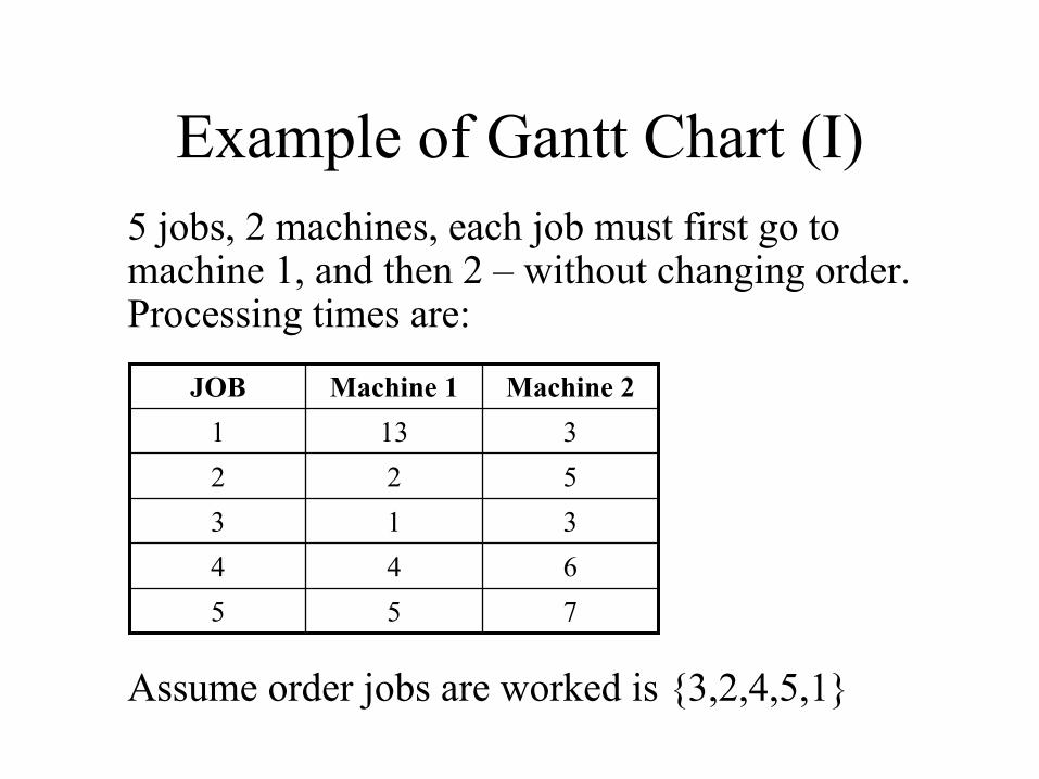
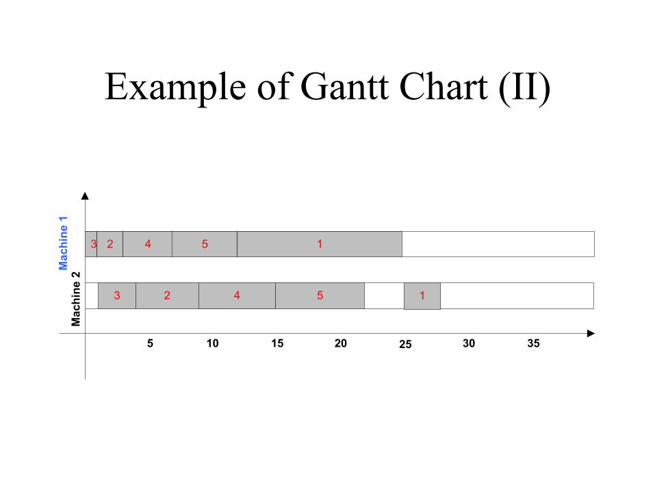
Example of Gantt Chart (I)5 jobs, 2 machines, each job must first go to machine 1, and then 2 – without changing order. Processing times are:

Assume order jobs are worked is {3,2,4,5,1}

7556443135223131

Machine 2Machine 1JOB

Example of Gantt Chart (II)

5 10 15 20 25 30 35

3

3

2 4 5 1

2 4 5 1

Mac

hine

1M

achi

ne 2

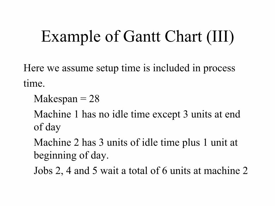
Example of Gantt Chart (III)

Here we assume setup time is included in processtime.

Makespan = 28Machine 1 has no idle time except 3 units at end of dayMachine 2 has 3 units of idle time plus 1 unit at beginning of day.Jobs 2, 4 and 5 wait a total of 6 units at machine 2

Scheduling Solutions

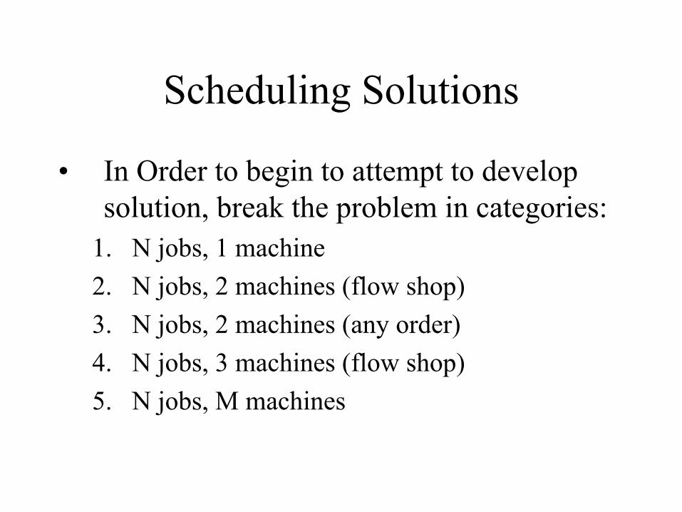
• In Order to begin to attempt to develop solution, break the problem in categories:

1. N jobs, 1 machine2. N jobs, 2 machines (flow shop)3. N jobs, 2 machines (any order)4. N jobs, 3 machines (flow shop)5. N jobs, M machines

Scenario 1 – n jobs, 1 machine (I)

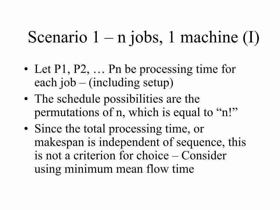
• Let P1, P2, … Pn be processing time for each job – (including setup)

• The schedule possibilities are the permutations of n, which is equal to “n!”

• Since the total processing time, or makespan is independent of sequence, this is not a criterion for choice – Consider using minimum mean flow time

Scenario 1 – n jobs, 1 machine (II)

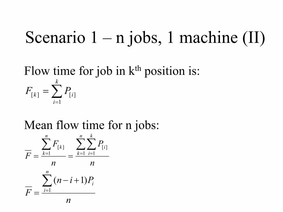
Flow time for job in kth position is:

Mean flow time for n jobs:

∑=

=k

iik PF

1][][

n

P

n

FF

n

k

k

ii

n

kk ∑∑∑

= == == 1 1][

1][

n

PinF

n

ii∑

=

+−= 1

)1(

Scenario 1 – n jobs, 1 machine (III)

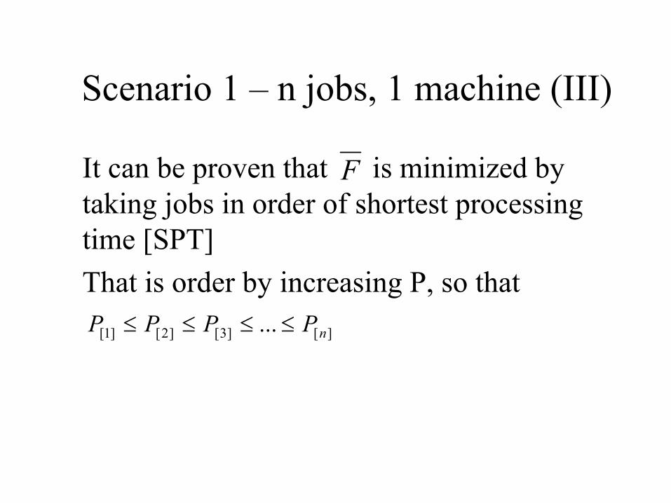
It can be proven that is minimized by taking jobs in order of shortest processing time [SPT]That is order by increasing P, so that

F

][]3[]2[]1[ ... nPPPP ≤≤≤≤

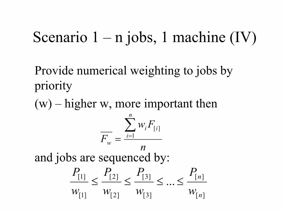
Scenario 1 – n jobs, 1 machine (IV)

Provide numerical weighting to jobs by priority(w) – higher w, more important then

and jobs are sequenced by:n

FwF

n

iii

w

∑== 1

][

][

][

]3[

]3[

]2[

]2[

]1[

]1[ ...n

n

wP

wP

wP

wP

≤≤≤≤

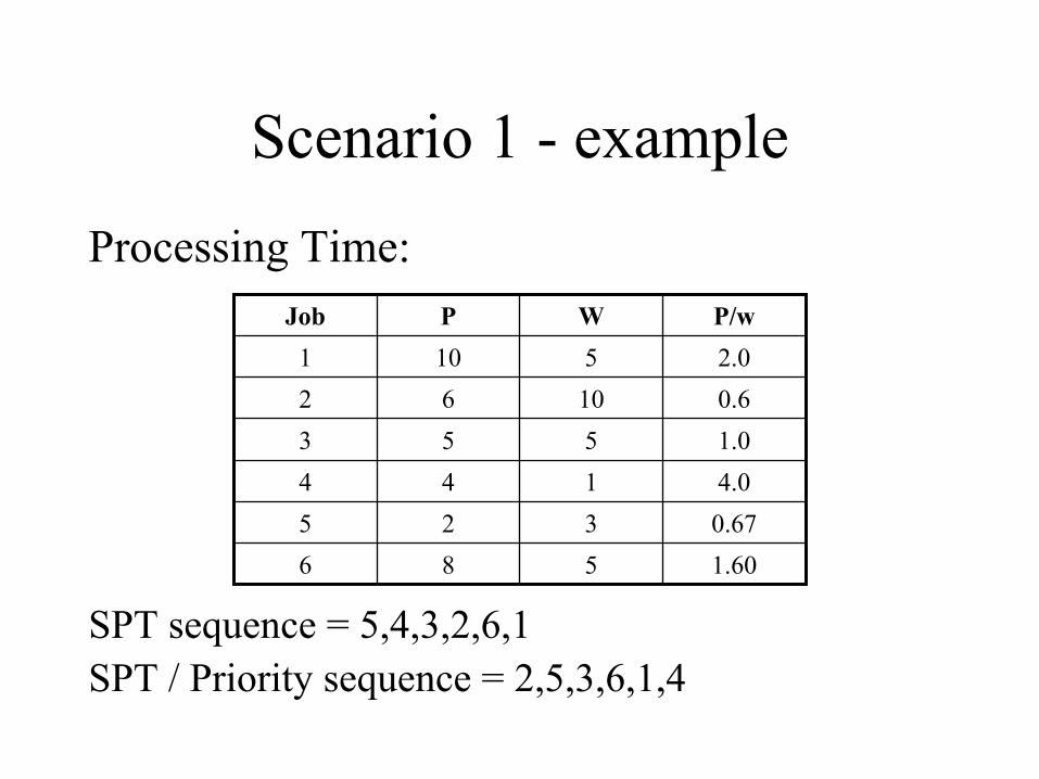
Scenario 1 - example

SPT sequence = 5,4,3,2,6,1SPT / Priority sequence = 2,5,3,6,1,4

1.605860.673254.01441.05530.610622.05101P/wWPJob

Processing Time:

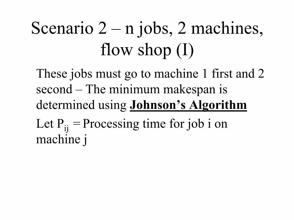
Scenario 2 – n jobs, 2 machines, flow shop (I)

These jobs must go to machine 1 first and 2 second – The minimum makespan is determined using Johnson’s AlgorithmLet Pij = Processing time for job i on machine j

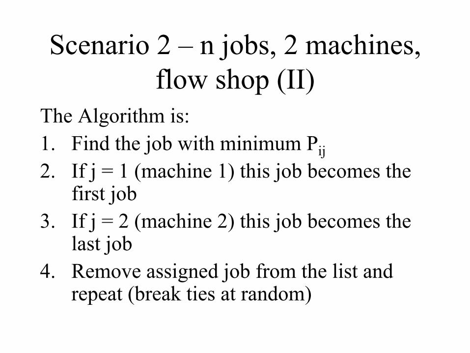
Scenario 2 – n jobs, 2 machines, flow shop (II)

The Algorithm is:1. Find the job with minimum Pij2. If j = 1 (machine 1) this job becomes the

first job3. If j = 2 (machine 2) this job becomes the

last job4. Remove assigned job from the list and

repeat (break ties at random)

Scenario 2 – n jobs, 2 machines, flow shop (III)

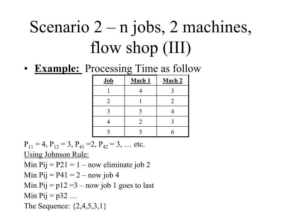
• Example: Processing Time as follow

655

324

453

212

341

Mach 2Mach 1Job

P11 = 4, P12 = 3, P41 =2, P42 = 3, … etc.Using Johnson Rule:Min Pij = P21 = 1 – now eliminate job 2Min Pij = P41 = 2 – now job 4Min Pij = p12 =3 – now job 1 goes to lastMin Pij = p32 …The Sequence: {2,4,5,3,1}

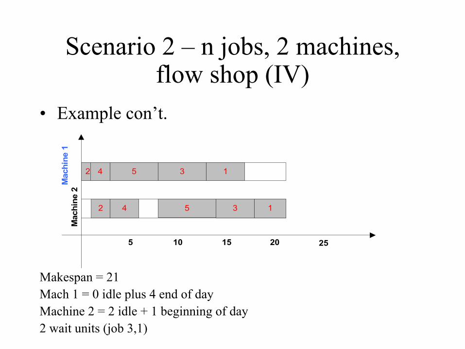
• Example con’t.

Scenario 2 – n jobs, 2 machines, flow shop (IV)

5 10 15 20 25

2

2

4 5 3 1

4 5 3 1

Mac

hine

1M

achi

ne 2

Makespan = 21Mach 1 = 0 idle plus 4 end of dayMachine 2 = 2 idle + 1 beginning of day2 wait units (job 3,1)

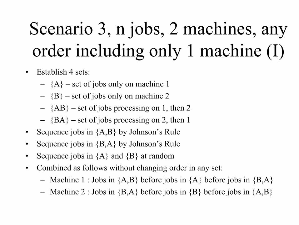
Scenario 3, n jobs, 2 machines, any order including only 1 machine (I)

• Establish 4 sets:– {A} – set of jobs only on machine 1– {B} – set of jobs only on machine 2– {AB} – set of jobs processing on 1, then 2– {BA} – set of jobs processing on 2, then 1

• Sequence jobs in {A,B} by Johnson’s Rule• Sequence jobs in {B,A} by Johnson’s Rule• Sequence jobs in {A} and {B} at random• Combined as follows without changing order in any set:

– Machine 1 : Jobs in {A,B} before jobs in {A} before jobs in {B,A}– Machine 2 : Jobs in {B,A} before jobs in {B} before jobs in {A,B}

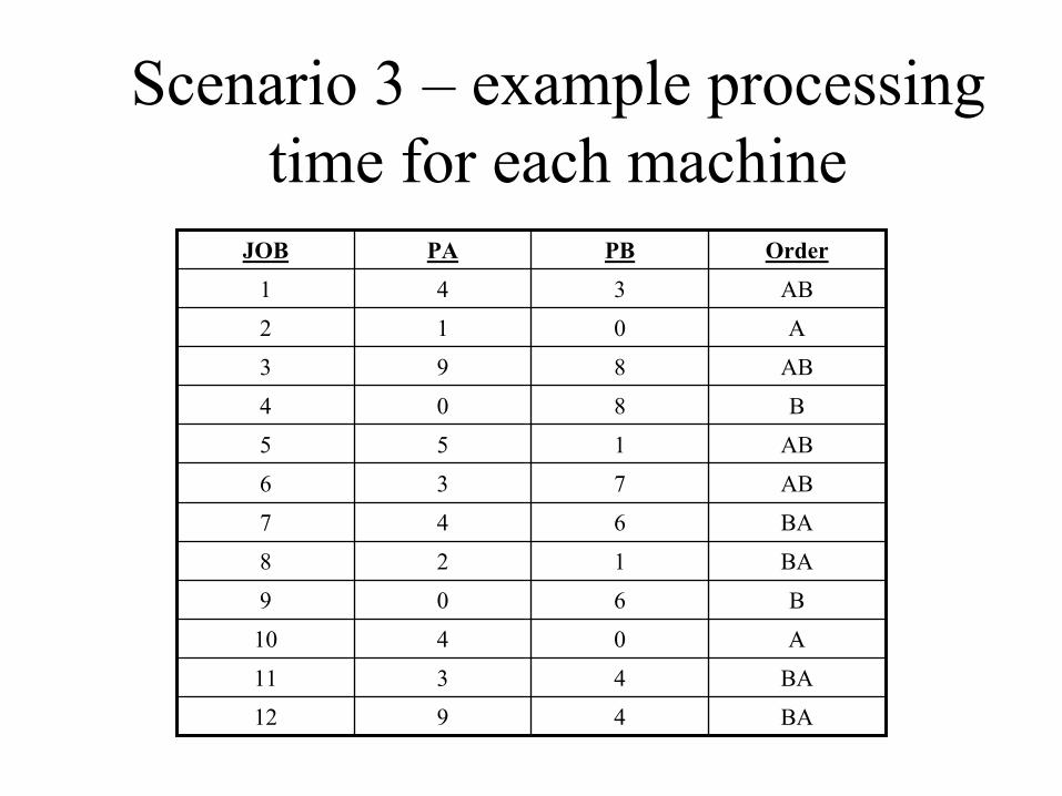
Scenario 3 – example processing time for each machine

BA4912

BA4311

A0410

B609

BA128

BA647

AB736

AB155

B804

AB893

A012

AB341

OrderPBPAJOB

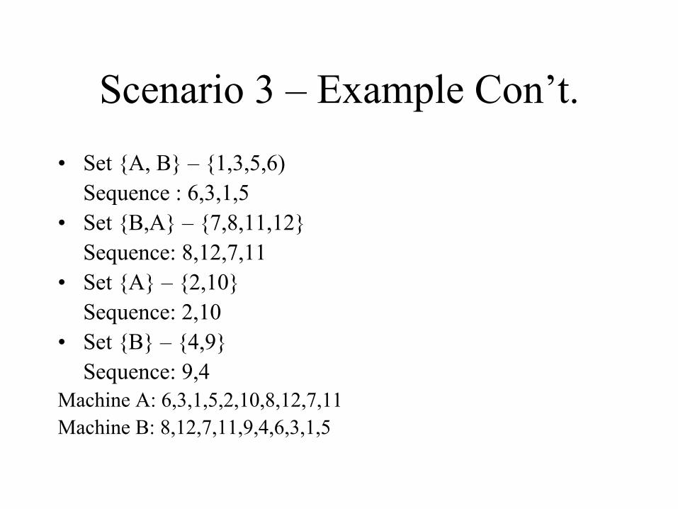
Scenario 3 – Example Con’t.• Set {A, B} – {1,3,5,6)

Sequence : 6,3,1,5• Set {B,A} – {7,8,11,12}

Sequence: 8,12,7,11• Set {A} – {2,10}

Sequence: 2,10• Set {B} – {4,9}

Sequence: 9,4Machine A: 6,3,1,5,2,10,8,12,7,11Machine B: 8,12,7,11,9,4,6,3,1,5

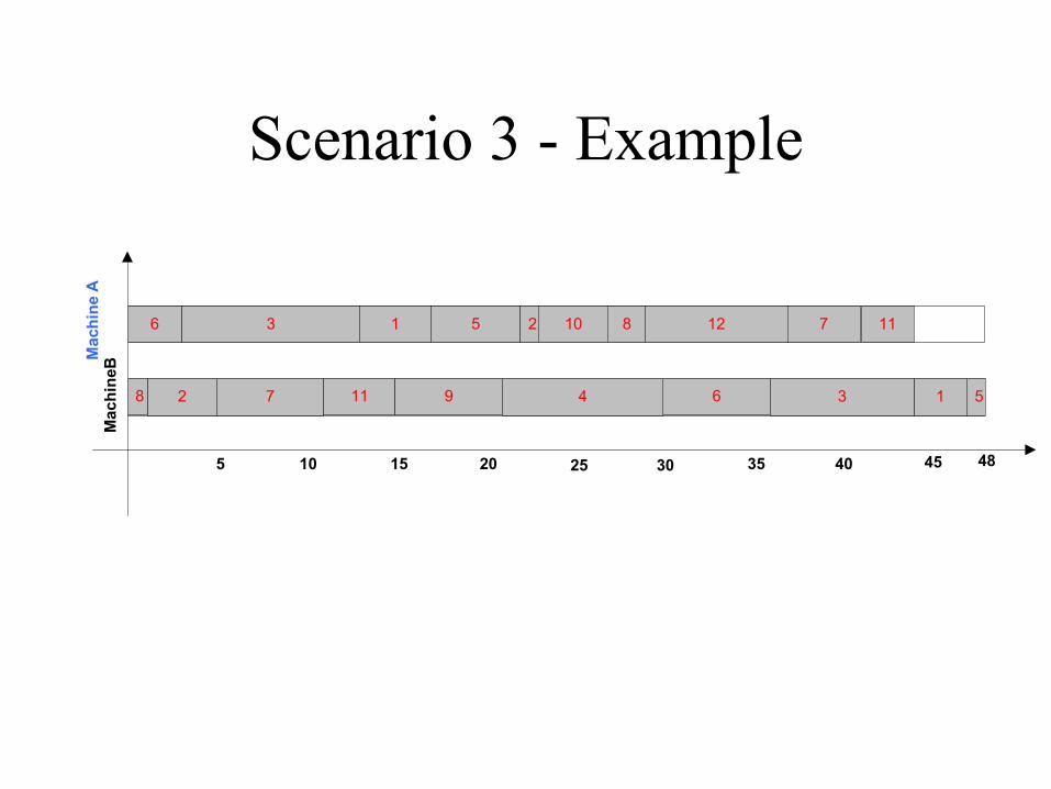
Scenario 3 - Example

5 10 15 20 25

6

2

3 1 5 2

7 11 9 1

30 35 40 45

53

11

48

712

648

810

Mac

hine

AM

achi

neB

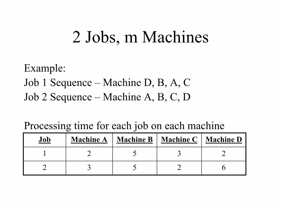
2 Jobs, m Machines

Example:Job 1 Sequence – Machine D, B, A, CJob 2 Sequence – Machine A, B, C, D

Processing time for each job on each machine

62532

23521

Machine DMachine CMachine BMachine AJob

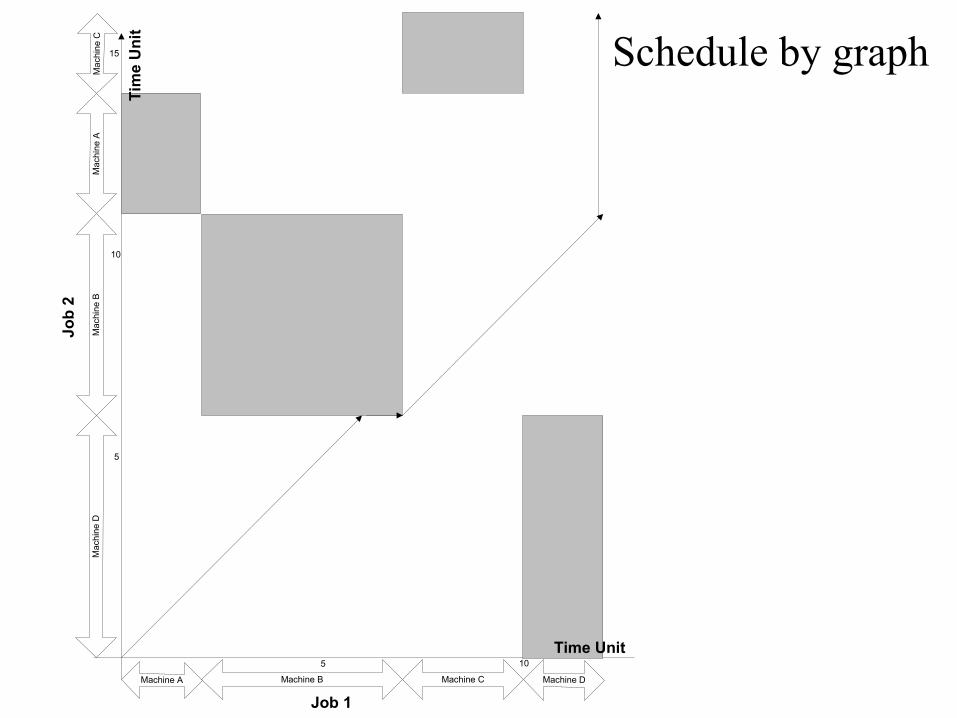
Job 1Machine A Machine B Machine C Machine D

5 10

Mac

hine

DM

achi

ne B

Mac

hin e

AM

achi

n e C

5

10

15

Job

2

Time Unit

Tim

e U

nit

Schedule by graph

N Jobs, M Machines

Number of possible schedules is extremely large, (n!)m

Almost all solved by heuristics which are based on sequencing or dispatching rules.

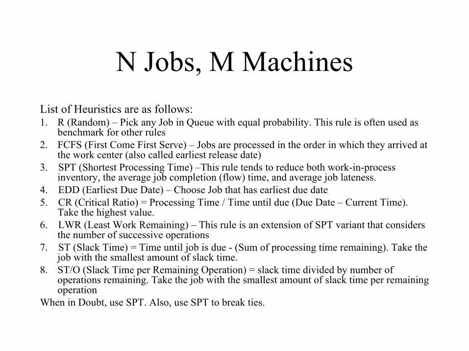
N Jobs, M MachinesList of Heuristics are as follows:1. R (Random) – Pick any Job in Queue with equal probability. This rule is often used as

benchmark for other rules2. FCFS (First Come First Serve) – Jobs are processed in the order in which they arrived at

the work center (also called earliest release date)3. SPT (Shortest Processing Time) –This rule tends to reduce both work-in-process

inventory, the average job completion (flow) time, and average job lateness.4. EDD (Earliest Due Date) – Choose Job that has earliest due date5. CR (Critical Ratio) = Processing Time / Time until due (Due Date – Current Time).

Take the highest value.6. LWR (Least Work Remaining) – This rule is an extension of SPT variant that considers

the number of successive operations7. ST (Slack Time) = Time until job is due - (Sum of processing time remaining). Take the

job with the smallest amount of slack time.8. ST/O (Slack Time per Remaining Operation) = slack time divided by number of

operations remaining. Take the job with the smallest amount of slack time per remaining operation

When in Doubt, use SPT. Also, use SPT to break ties.