Trade Liberalization and Unemployment:

Theory and Evidence from India

Rana Hasan

Asian Development Bank rhasan@adb.org

Devashish Mitra Syracuse University

dmitra@maxwell.syr.edu

Priya Ranjan University of California - Irvine

pranjan@uci.edu

Reshad N Ahsan University of Melbourne rahsan@unimelb.edu.au

December, 2010

Abstract

A widely held view among the public is that trade liberalization increases unemployment. In this paper we use state- and industry-level data on unemployment rates and trade protection from India to examine what the data say. We find little evidence to support the view that unemployment rises with trade liberalization. On the contrary, our analysis suggests that to the extent there is a statistically significant relationship, unemployment declines with trade liberalization in certain contexts. In particular, our state-level analysis reveals that urban unemployment declines with liberalization in states with more flexible labor markets and larger employment shares in net exporter industries. Moreover, our industry-level analysis indicates that workers in industries experiencing greater reductions in trade protection were less likely to become unemployed, especially in net export industries. There is some weak evidence that the short-run impact of a tariff reduction may be a quick increase in unemployment prior to reduction to a lower steady-state unemployment rate. Our results can be explained using a theoretical framework incorporating trade and search-generated unemployment and some institutional features of the Indian economy.

# We thank seminar particiapants at the University of Adelaide, the University of Auckland, the University of Melbourne, the University of New South Wales, the University of Otago and the University of Sydney for very useful comments and suggestions. J. Salcedo Cain provided excellent research assistance on this project. We also thank Deb Kusum Das for developing some of the data on trade protection used by us. The work of both was supported by an ADB technical assistance project (RETA 6364: Measurement and Policy Analysis for Poverty Reduction). The paper represents the views of the authors and does not necessarily represent those of the Asian Development Bank, its Executive Directors, or the countries that they represent. The standard disclaimer applies. Corresponding author: Department of Economics, The Maxwell School, Syracuse University, Eggers Hall, Syracuse, NY 13244. Phone: (315) 443-6143, Fax: (315) 443-3717.

1

1. Introduction

There now exists a small but growing literature on the relationship between trade and unemployment.1 Most

of this literature is theoretical with some exceptions. One exception is Dutt, Mitra and Ranjan (2009).2 Using

cross-country data on trade policy, unemployment, and various controls, and controlling for endogeneity and

measurement-error problems, they find that unemployment and trade openness are negatively related. Using

panel data, they find an unemployment-increasing short-run impact of trade liberalization, followed by an

unemployment-reducing effect leading to the new steady state. While that paper finds interesting empirical

regularities that can be explained using plausible models of trade and search unemployment, the standard

criticisms of cross-country regressions apply to that study as well. Countries differ from each other in very

important ways that cannot always be controlled for by variables we use in such regressions. Therefore, we

begin our analysis by going down to the next level from cross-country analysis – i.e., to an intra-country

analysis of state-level and industry-specific unemployment derived from "employment-unemployment"

surveys carried out by India's National Sample Survey Organisation (NSSO). India is a developing country

that has, in the last couple of decades, experienced major trade reforms and where a significant proportion of

the population lives below the poverty line. This makes such a study potentially quite useful for policy

analysis.

Importantly, constitutional arrangements which give India’s states considerable regulatory power

over economic matters and the large size of India’s states – many of which have populations larger than the

vast majority of countries and possess unique ethno-linguistic characteristics – make such an analysis

meaningful. In particular, interstate variations in labor regulations (see Besley and Burgess, 2004) and low

mobility across Indian states (see Dyson Cassen, and Visaria, 2004 and Topalova, 2010) suggest that treating

1 The most prominent contributors to this literature are Carl Davidson and Steve Matusz. See Davidson et al. (1999) for a representative work and Davidson and Matusz (2004) for a survey. Also see Moore and Ranjan (2005) and Mitra and Ranjan (2010) for recent contributions to this literature. 2 Another exception is some analysis of the correlation between job destruction and net exports across sectors in chapter 4 of the book by Davidson and Matusz (2004). They find a negative correlation between the two (equivalent to a positive correlation between net imports and job destruction), and perform some further regressions to look deeper into this correlation. See Davidson and Matusz (2005) for a more detailed empirical analysis.

2

each state as an independent labor market is a reasonable approximation. Additionally, we adopt broadly the

strategy of Topalova (2007) and Hasan, Mitra, and Ural (2007) and exploit variations in industrial

composition across Indian states (districts in the case of Topalova) around the time of the major trade

liberalization of the early 1990s, and the variation in the degree of liberalization across industries over time to

construct state-specific measures of protection. This allows us to determine whether states more exposed to

reductions in protection experienced increases or decreases in unemployment rates.

We then complement our cross-state analysis of the relationship between unemployment and

liberalization with a detailed analysis based purely on changes in industry-level variations in protection over

time. More specifically, we examine whether workers in industries experiencing greater reductions in trade

protection were more or less likely to become unemployed. We also check what this relationship looks like in

the presence of controls for other elements of India’s policy reforms.

Insofar as our state-level analysis is concerned, we find that overall (rural plus urban) unemployment

on average does not have any relationship with average protection (weighted average with 1993 sectoral

employment as weights) over time and across states. However, there are some conditional relationships

between the two variables in certain types of states. In states with more flexible labor markets, there is

evidence that on average overall and urban unemployment are positively related to protection. In other

words, trade liberalization there can reduce unemployment. We also find that reductions in protection reduce

unemployment in the urban sectors of states with large employment shares in net exporter industries. Across

such states and within such states over time, the employment-weighted protection and unemployment are

positively correlated. This is true across all the three measures of protection we use.

Turning to our analysis based purely on industry-level protection, we find hardly any evidence that

workers in industries that experienced larger reductions in protection were more likely to be unemployed. In

fact, there seems to be some evidence to the contrary that such workers could actually have been less likely to

become unemployed, a result that is stronger in net exporter industries. There is some weak evidence that the

immediate short-run effect of a tariff reduction may be an increase in unemployment prior to reduction to a

lower steady-state unemployment rate (long-run fall in the unemployment rate).

3

We show how our empirical results are consistent with the impact of trade liberalization in a two

sector model, with labor being the only factor of production and where unemployment arises due to search

frictions.3 We discuss two extreme cases: (a) perfect labor mobility (the Ricardian case), where comparative

advantage is exclusively productivity-driven and (b) no intersectoral labor mobility (where labor becomes

sector-specific), where comparative advantage, while still dependent on productivity, is also driven by relative

sectoral labor force size. Our empirical results fall in between the two extremes, depending on the flexibility

of labor markets. The results get closer to the predictions of the model with perfect intersectoral labor

mobility as we move from states with rigid labor laws to those with labor laws that lead to more flexible labor

markets.

It must be pointed out here that our empirical results can also be related to the predictions of some

other theoretical models in the trade and unemployment literature. While an unemployment reducing effect

of trade liberalization, through an aggregate productivity effect based on firm selection, is obtained in the

theoretical work of Felbermayr, Prat and Schmerer (2008), the opposite result is possible in Helpman and

Itskhoki (2010). To the extent that trade, in the two-sector model by Helpman and Itskhoki, leads to higher

aggregate productivity in their differentiated products sector subject to search frictions, this sector expands in

size and the other sector, which is frictionless and has zero unemployment as a result, shrinks. A similar result

is also obtained in Janiak (2007). There are other papers in the literature, such as Davidson, Martin and

Matusz (1999) and Moore and Ranjan (2005) where the effect of trade on overall unemployment is

ambiguous.4

In the next section (section 2), we present a theoretical framework to guide us in our empirical

analysis. In section 3, we discuss the Indian policy framework. This is followed by our empirical strategy in

section 4, the data in section 5 and the empirical results in section 6. We finally end with some concluding

remarks in section 7.

3 It is also shown that the theoretical results are robust to modeling unemployment through efficiency wages as in Shapiro and Stiglitz (1984). 4 In Davidson, Martin and Matusz the results depend on intersectoral and international differences in labor-market frictions. In Moore and Ranjan, there are two kinds of labor (skilled and unskilled) and the effects of trade on the unemployment of these two kinds of workers go in opposite directions, making the impact on overall unemployment ambiguous.

4

2. Trade and Unemployment: Theoretical Framework

Production Structure

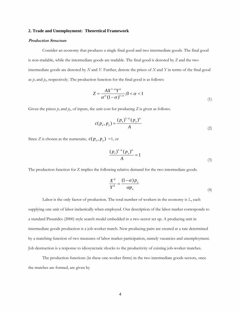
Consider an economy that produces a single final good and two intermediate goods. The final good

is non-tradable, while the intermediate goods are tradable. The final good is denoted by Z and the two

intermediate goods are denoted by X and Y. Further, denote the prices of X and Y in terms of the final good

as px and py, respectively. The production function for the final good is as follows:

10;

)1( 1

1

YAXZ

(1)

Given the prices px and py, of inputs, the unit cost for producing Z is given as follows.

A

ppppc yx

yx

)()(),(

1

(2)

Since Z is chosen as the numeraire, ),( yx ppc =1, or

1

)()( 1

A

pp yx

(3)

The production function for Z implies the following relative demand for the two intermediate goods.

x

y

d

d

p

p

Y

X

)1(

(4)

Labor is the only factor of production. The total number of workers in the economy is L, each

supplying one unit of labor inelastically when employed. Our description of the labor market corresponds to

a standard Pissarides (2000) style search model embedded in a two sector set up. A producing unit in

intermediate goods production is a job-worker match. New producing pairs are created at a rate determined

by a matching function of two measures of labor market participation, namely vacancies and unemployment.

Job destruction is a response to idiosyncratic shocks to the productivity of existing job-worker matches.

The production functions (in these one-worker firms) in the two intermediate goods sectors, once

the matches are formed, are given by

5

yyxx lhylhx ; (5)

If Li is the total number of workers affiliated with sector-i, ui the unemployment rate in sector-i, then the

number of employed in sector-i is (1- ui) Li. The aggregate production in each sector is given by

LLLLuhYLuhX yxyyyxxx ;)1(;)1( (6)

The relative supply of the two intermediate goods is

yyy

xxxs

s

Luh

Luh

Y

X

)1(

)1(

(7)

The total number of matches in the labor market is determined by the matching technology given as

follows. Let vi be the vacancy rate (i.e., the number of vacancies divided by the labor force) in sector-i. Define

θi= vi/ui as a measure of market tightness, and let mi be a scale parameter in the matching function. Then,

write the flow of matches in each sector per unit time as follows:

10;)()()(),( 1 iiiiiiiiiiiii LumLuvmLuLvM (8)

where γ is a parameter capturing the vacancy intensity of this Cobb-Douglas matching function. Then, the

exit rate (from unemployment) for an unemployed searcher in sector-i is iiii

i mLu

M , and the rate at which

vacant jobs are filled is 1 iiii

i mLv

M. The former is an increasing function of market tightness, and the

latter is a decreasing function of market tightness. Assume that the matches in sector-i are broken at an

exogenous rate of λi per period. λi can be viewed as an arrival rate of a shock that leads to job destruction.

Given the above description of labor market, the net flow into unemployment per period of time is

iiiiii umuu )1( (9)

In the steady-state the rate of unemployment is constant. Therefore, the steady-state unemployment in sector-

i is given by

iii

ii m

u

(10)

6

Denote the recruitment cost in sector-i in terms of the final good by δi , the firing cost by Fi and the

exogenous discount factor by ρ. The asset value of a vacant job, Vi is characterized by the following Bellman

equation

)(1iiiii VJmV (11)

where Ji is the value of an occupied job. Free entry in job creation implies Vi = 0, which we set from now on.

Denoting the wage of workers in sector-i by wi in terms of the numeraire, the asset value of an occupied job,

Ji satisfies the following Bellman equation

)( iiiiiii FJwhpJ (12)

Note that when the job is destroyed, the firm not only loses Ji but also has to pay the firing cost Fi.

Free entry in job creation (Vi = 0) implies the following from (11) above.

1

i

ii m

J (13)

Equations (12) and (13) imply

1

)(

i

iiiiiii m

Fwhp (14)

The above is also a zero profit condition which says that the value of a match equals the wage plus the

expected hiring and firing costs.

Wage Determination

On the worker side, unemployed workers in each sector receive a flow benefit of b in units of the

final good. This "benefit" includes the value of leisure as well as unemployment insurance payments. Let Wi

denote the present discounted value of employment in sector i and Ui the present discounted value of

unemployment. The Bellman equations governing Wi and Ui are given by:

)( iiiii WUwW (15)

)( iiiii UWmbU (16)

Wage is determined through a process of Nash bargaining between the worker and the entrepreneur where

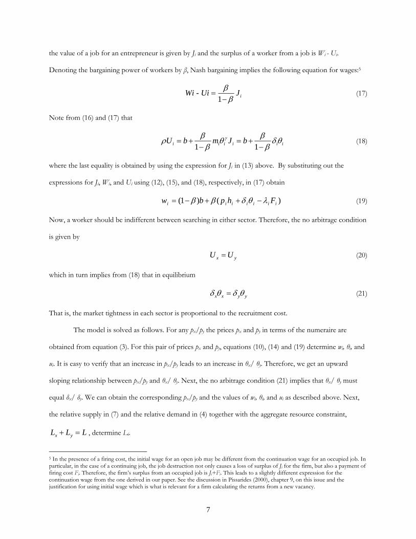
7

the value of a job for an entrepreneur is given by Ji and the surplus of a worker from a job is Wi - Ui.

Denoting the bargaining power of workers by β, Nash bargaining implies the following equation for wages:5

iJWi - Ui

1

(17)

Note from (16) and (17) that

iiiiii bJmbU

11 (18)

where the last equality is obtained by using the expression for Ji in (13) above. By substituting out the

expressions for Ji, Wi, and Ui using (12), (15), and (18), respectively, in (17) obtain

)()1( iiiiiii Fhpbw (19)

Now, a worker should be indifferent between searching in either sector. Therefore, the no arbitrage condition

is given by

yx UU (20)

which in turn implies from (18) that in equilibrium

yyxx (21)

That is, the market tightness in each sector is proportional to the recruitment cost.

The model is solved as follows. For any px/py the prices px and py in terms of the numeraire are

obtained from equation (3). For this pair of prices px and py, equations (10), (14) and (19) determine wi, θi, and

ui. It is easy to verify that an increase in px/py leads to an increase in θx/ θy. Therefore, we get an upward

sloping relationship between px/py and θx/ θy. Next, the no arbitrage condition (21) implies that θx/ θy must

equal δx/ δy. We can obtain the corresponding px/py and the values of wi, θi, and ui as described above. Next,

the relative supply in (7) and the relative demand in (4) together with the aggregate resource constraint,

LLL yx , determine Li.

5 In the presence of a firing cost, the initial wage for an open job may be different from the continuation wage for an occupied job. In particular, in the case of a continuing job, the job destruction not only causes a loss of surplus of Ji for the firm, but also a payment of firing cost Fi. Therefore, the firm’s surplus from an occupied job is Ji+Fi. This leads to a slightly different expression for the continuation wage from the one derived in our paper. See the discussion in Pissarides (2000), chapter 9, on this issue and the justification for using initial wage which is what is relevant for a firm calculating the returns from a new vacancy.

8

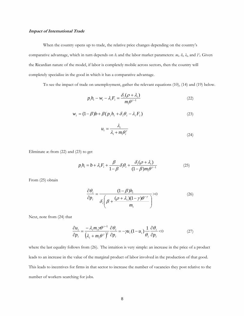
Impact of International Trade

When the country opens up to trade, the relative price changes depending on the country’s

comparative advantage, which in turn depends on hi and the labor market parameters: mi, δi, λi, and Fi. Given

the Ricardian nature of the model, if labor is completely mobile across sectors, then the country will

completely specialize in the good in which it has a comparative advantage.

To see the impact of trade on unemployment, gather the relevant equations (10), (14) and (19) below.

1

)(

i

iiiiiii m

Fwhp (22)

)()1( iiiiiii Fhpbw (23)

iii

ii m

u

(24)

Eliminate wi from (22) and (23) to get

1)1(

)(

1

i

iiiiiiii m

Fbhp (25)

From (25) obtain

i

ii

i

i

i

m

h

p

)1)((

)1(>0 (26)

Next, note from (24) that

i

i

iii

i

i

ii

ii

i

i

puu

pm

m

p

u

1)1(

2

1

<0 (27)

where the last equality follows from (26). The intuition is very simple: an increase in the price of a product

leads to an increase in the value of the marginal product of labor involved in the production of that good.

This leads to incentives for firms in that sector to increase the number of vacancies they post relative to the

number of workers searching for jobs.

9

Without loss of generality, suppose the country has a comparative advantage in good X. Trade in

this case will raise the relative price of X, which implies an increase in px and a decrease in py. Given the

Ricardian nature of the model, the no-arbitrage condition cannot be satisfied anymore and all labor will move

to sector X. It is clear from (27) above that the post-trade unemployment in sector X is lower than before.

The impact on the economy-wide unemployment depends on whether the X sector had higher or lower

unemployment to begin with. If the Y sector had lower unemployment to begin with, then the impact of

trade on economy-wide unemployment is ambiguous. Otherwise, trade reduces unemployment, including in

the neutral case with symmetric search friction across sectors (δx = δy), in which case under autarky both

sectors have the same unemployment rate.

In the more likely case of costly labor mobility (which could be due to loss of skills in moving from

one sector to another or some other idiosyncratic costs due to heterogeneity of preferences),6 the country

may remain incompletely specialized even after opening to trade and the no-arbitrage condition is satisfied for

the marginal worker. In this case, the unemployment rate decreases in sector X and increases in sector Y. The

net impact on economy-wide unemployment is going to be ambiguous, as the overall unemployment will be a

labor-force weighted average of the two sector-specific unemployment rates.

Using the logic we have developed so far, it is easy to see that in a multisectoral model, a tariff

reduction in an import competing sector, as long as that sector exists, will lead to an increase in the

unemployment rate within that sector. The reason is that a tariff reduction leads to a reduction in the

domestic price of that good and therefore to a reduction in the value of the marginal product of labor within

that sector.

In our empirical analysis, sectoral employment-unemployment status is available for all the rounds of

the survey we use only at the two-digit level. At this coarse level of disaggregation, it is difficult to

differentiate between import tariffs on output and inputs. The reason is that at this level of (dis)aggregation,

a high fraction of the input into a sector comes from itself. While we have not modeled the interaction

between labor working in a sector in combination with a complementary input being used in the same sector,

6 See Mitra and Ranjan (2010) for the impact of offshoring on unemployment in a search model with mobility cost.

10

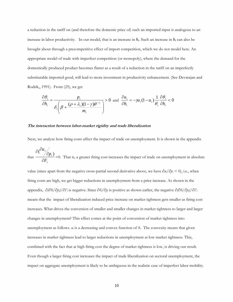
a reduction in the tariff on (and therefore the domestic price of) such an imported input is analogous to an

increase in labor productivity. In our model, that is an increase in hi. Such an increase in hi can also be

brought about through a precompetitive effect of import competition, which we do not model here. An

appropriate model of trade with imperfect competition (or monopoly), where the demand for the

domestically produced product becomes flatter as a result of a reduction in the tariff on an imperfectly

substitutable imported good, will lead to more investment in productivity enhancement. (See Devarajan and

Rodrik,, 1991). From (25), we get

0)1)((

i

ii

i

i

i

m

p

h

and 0

1)1(

i

i

iii

i

i

huu

h

u

The interaction between labor-market rigidity and trade liberalization

Next, we analyze how firing costs affect the impact of trade on unemployment. It is shown in the appendix

that i

i

i

F

pu

)(<0. That is, a greater firing cost increases the impact of trade on unemployment in absolute

value (since apart from the negative cross-partial second derivative above, we have ∂ui/∂pi < 0), i.e., when

firing costs are high, we get bigger reductions in unemployment from a price increase. As shown in the

appendix, ∂(∂θi/∂pi)/∂Fi is negative. Since ∂θi/∂pi is positive as shown earlier, the negative ∂(∂θi/∂pi)/∂Fi

means that the impact of liberalization induced price increase on market tightness gets smaller as firing cost

increases. What drives the conversion of smaller and smaller changes in market tightness to larger and larger

changes in unemployment? This effect comes at the point of conversion of market tightness into

unemployment as follows. ui is a decreasing and convex function of θi. The convexity means that given

increases in market tightness lead to larger reductions in unemployment at low market tightness. This,

combined with the fact that at high firing cost the degree of market tightness is low, is driving our result.

Even though a larger firing cost increases the impact of trade liberalization on sectoral unemployment, the

impact on aggregate unemployment is likely to be ambiguous in the realistic case of imperfect labor mobility.

11

This is because a higher F should cause a larger increase in unemployment in the import competing sector

and a larger decrease in unemployment in the export sector. Thus the effect of firing costs on how

unemployment responds to trade liberalization is an empirical one. In our empirical work in this paper, this is

related to the issue of the variation in labor market rigidity coming from the variation in labor laws across the

different Indian states. The states with more pro-employee labor laws are the ones that are considered to have

more rigid labor laws where we can think of firms face higher firing costs. In addition, these pro-employee

laws increase bargaining power of workers, which increases wage, but that reduces labor market tightness and

increases sectoral unemployment. Furthermore, we can show in our model (where the rate of job destruction

is exogenous) that ∂(∂θi/∂pi)/∂β < 0, but because unemployment is convex and decreasing in market

tightness ∂(∂ui/∂pi)/∂β can be shown to have an ambiguous sign in our model.

Short-run effects

Even though we discuss only the steady-state implication of trade liberalization on unemployment, we can get

some idea of the impact effect by looking at equation (9) which gives the expression for the change in

unemployment over time which we recall is

iiiiii umuu )1(.

Trade liberalization in our set up affects unemployment mainly through changes job creation captured by the

second term on the right hand side in the above expression. In one sector , job creation goes up and in the

other sector it goes down (with the market tightness being a jump variable). This leads to the possibility of the

overall unemployment rate adjusting non-monotonically even if it increases monotonically in the import

competing sector and decreases monotonically in the export sector.

Going beyond the model, if job creation takes time while job destruction is instantaneous, then

following trade liberalization the unemployment in the export sector will decrease gradually, while the

unemployment in the import competing sector will increase rapidly. Because of this asymmetry in the time

taken in job creation and job destruction, it is possible for unemployment to increase in the short run, and

decrease in the long run. As well, in the case of costly labor mobility, less workers are likely to move from the

12

contracting sector to the expanding sector in the short run than in the long run. This would be another force

creating an increase in unemployment in the short run followed by a decrease in the long run.

3. The Indian Policy and Institutional Framework

We next provide an overview of the Indian regulatory and institutional framework, an understanding of

which is important for the analysis we undertake in this paper. There are two features of the Indian policy

landscape that have an important bearing on the strategy we adopt for estimating the impact of trade

protection on unemployment rates. First, notwithstanding some earlier efforts, India undertook a dramatic

liberalization of trade policies in 1991. Thus, for example, mean tariffs, which were 128 percent before July

1991, had fallen to roughly 35 percent by 1997-98 and the standard deviation of tariffs during this period

went down from 41 percentage points to roughly 15. Significantly, the trade liberalization was unanticipated.

It was the result of strong conditionality imposed by the International Monetary Fund (IMF) in return for

IMF assistance for dealing with a balance of payments crisis. Given several earlier attempts to avoid IMF

loans and the associated conditionalities, the liberalization came as a surprise.7 Given its large and

unanticipated nature, the trade liberalization of 1991 presents researchers an excellent opportunity to examine

the effects of trade using data on trade protection and variables whose relationship with trade we are

interested in examining spanning the years prior to 1991 and later.8

Second, the impact of India's trade liberalization on unemployment can be expected to vary across

Indian states. One reason is that the degree to which states are exposed to trade protection is unlikely to be a

constant. In particular, the composition of employment across industries will typically vary across states

7 In addition to the reduction of tariff levels and their dispersion, trade liberalization involved the removal of most licensing and other non-tariff barriers on all imports of intermediate and capital goods, the broadening and simplification of export incentives, the removal of export restrictions, the elimination of the trade monopolies of the state trading agencies, and the simplification of the trade regime. Trade liberalization was also accompanied by full convertibility of the domestic currency for foreign exchange transactions. See Hasan, Mitra, and Ramaswamy (2007) and the sources cited therein for more details. 8 See also the discussion in Topalova (2007) and (2004a) on the extent to which India's trade liberalization was an endogenous outcome of political and economic processes. In particular, Topalova’s analysis indicates that at least until 1996 , the variation in reductions in protection across industries was unlikely to be driven by economic and political factors that would give rise to concerns about trade policy variables being endogenous in our empirical analysis.

13

thereby leading states to be differentially exposed to trade liberalization. Another reason has to do with the

fact that the regulatory environment varies across India's states.9 To the extent that the effects of trade

liberalization are influenced by the nature of the regulatory environment in which economic activity takes

place, the impact of trade liberalization on unemployment can be expected to vary across India's states.

An element of regulation that is especially relevant for the analysis of this paper is labor market

regulation. Under the Indian constitution, both the central (federal) government as well as individual state

governments have the authority to legislate on labor related issues. In fact, the latter have the authority to

amend central legislations or to introduce subsidiary legislations. In addition, the enforcement of many labor

regulations, even those enacted by the central government, lies with the state governments.10 Thus, the

placement of labor issues in the Indian constitution suggests variation in labor regulations and/or their

enforcement across India’s states. It is important to take into account this variation in assessing the impact of

trade liberalization on unemployment given the considerable debate among analysts regarding the effects of

labor market regulations, especially certain elements of the Industrial Disputes Act (IDA) which makes it

necessary for firms employing more than 100 workers to obtain the permission of state governments in order

to retrench or lay off workers -- permission which some analysts argue is rarely forthcoming and thereby ends

up raising the effective cost of labor usage in production.11

4. Empirical Strategy

We analyze the relationship between trade protection and unemployment using two empirical strategies. A

first strategy is along the lines of Topalova (2007) and Hasan, Mitra, and Ural (2007)- both of which examine

the relationship between trade liberalization and poverty- and exploits variation in the extent of openness

across India's states to identify the effects of trade liberalization on unemployment rates. A second strategy

exploits variation in the extent of protection across industries and over time to determine whether industries 9 This is because India's constitution gives its states control over various areas of regulation. In these areas, states have the authority to enact their own laws and amend legislations passed by the Central (federal) government. Typically, states also have the authority to decide on the specific administrative rules and procedures for enforcing legislations passed by the center. 10 See Anant et al (2006) for a detailed discussion of India’s labor-market regulations. 11 A similar case could be made for other types of regulation -- for example, product market regulations. We discuss this possibility in more detail later.

14

experiencing greater reductions in protection saw greater unemployment among their workers. This strategy

closely follows that of Attanasio, Goldberg, and Pavcnik (2004) and is also related to the approach of

Menezes-Filho and Muendler (2006).

4.1 State-Level Analysis

In the context of the foregoing discussion, our strategy for estimating the impact of trade protection on state

unemployment relies on estimating variants of the following basic regression specification:

ittii

jit

jit

jit regulationprotectionprotectiony *ln 1211 (33)

where yjit is the natural logarithm of the unemployment rate in state i and sector j (i.e., for the state as a whole

or a state's rural sector or its urban sector), protectionjit-1 refers to a measure of state-level trade protection

(explained later) lagged once per state i and sector j in order to alleviate concerns about endogeneity and for

allowing time for unemployment to respond to protection, and regulationi is a time-invariant variable capturing

the stance of regulations across states. i represents fixed state effects, t represents year dummies, and εit

represents an identically and independently distributed error term.

The effect of trade liberalization on unemployment can be gauged by considering the marginal effect

of protection on unemployment. This is the sum of two terms: β1 + β2 · regulation. The first-term represents

the direct effect of trade protection on unemployment. Ignoring the second term, a positively signed estimate

of β1 implies that reductions (increases) in protection are associated with reductions (increases) in the

unemployment rate. However, the nature of regulations may influence how protection affects

unemployment. The term β2 -- the coefficient on the interaction between our measures of protection and

state-level regulations -- is designed to capture this. Suppose, for example, that regulation is a dummy variable

capturing whether or not labor market regulations are flexible (pro-business) or not across Indian states. A

positively signed estimate of β2 implies that reductions (increases) in protection are associated with bigger

reductions (smaller increases) in unemployment in states with flexible (inflexible) labor market regulations.

Of course, the total effect of trade liberalization will depend on the sum of the two terms and vary across

states.

15

It needs to be acknowledged that the validity of the above inferences would weaken in the face of interstate

migration of workers. For example, unemployed individuals in states with flexible labor regulations and

experiencing large declines in trade protection, may move out of such states. A positively signed estimate of

β2 may then be at least partly driven by such movements of workers.12 Fortunately for our analysis, India is a

country with relatively low migration rates. As borne out by the detailed work of Dyson Cassen, and Visaria

(2004) using decennial population census data, the bulk of migration in India occurs among women on

account of marriage; mobility for economic reasons is limited. Moreover, the migration that occurs, does so

mostly within and across districts and very seldom across states. In fact, interstate migration has been

declining in recent decades.13 These considerations strongly suggest that our results are unlikely to be driven

by changes in the composition of the workforce at the state level.

4.2 Industry-Level Analysis

We next turn to our industry-level analysis. While the data available to us does not describe the industry in

which unemployed workers are seeking employment, they do inform us about their most recent previous

industry of employment (if any). This allows us to focus on the effect of trade protection on the probability

that a worker with previous work experience in a given industry has become unemployed. To do so we

employ the two-stage approach used by Attanasio, Goldberg, and Pavcnik (2004) and Goldberg and Pavcnik

(2005). This approach is based on the industry wage premium methodology used in the labor literature. In the

First stage, we estimate the following equation:

3it i it s k itunemployed a X e (34)

where unemployedjt is an indicator variable that is 1 for workers with previous experience who have been

become unemployed and 0 otherwise. Xjt captures individual characteristics such as age, age squared,

dummies for male workers, rural workers, and indicator variables for educational status. γs are state dummies

12 We are grateful to a referee for not only pointing this out, but also for directing us to some of the relevant literature. 13 Admittedly, the low estimates of migration reported in the decennial census may underestimate economic migration of shorter duration, as well as circulatory migration between rural and urban areas. Recent surveys by the NSSO have sought to capture some of these dimensions by applying a tighter definition than that allowed by census data. According to these surveys, the levels of migration are going up, but it is hard to discern an acceleration in migration in recent decades, especially across states (Anant et al, 2006). Low labor mobility across Indian states is also clearly pointed to in the work of Munshi and Rosenzweig (2007) and Topalova (2010).

16

while γk are industry dummies. For unemployed workers γk captures the immediate past industry in which

they worked. Finally eit is an identically and independently distributed error term.

The industry dummy variable coefficients represent the part of the probability of unemployment that

cannot be explained by individual characteristics and are instead due to a worker’s industry affiliation.

Obtaining industry measures of the probability of unemployment in this manner is advantageous since the

individual characteristics above control for composition differences (based on age, education etc) across

industries. This ensures that the relationship between the probability of unemployment and trade protection

in the second stage are not driven by such compositional differences.

As is the case in the previous literature (see Attanasio, Goldberg, and Pavcnik, 2004 and Goldberg

and Pavcnik, 2005), we normalize our industry coefficients by converting them to a deviation from an

employment-weighted average industry probability of unemployment. The normalized industry coefficients

thus represent the probability of becoming unemployed in an industry relative to that probability in an

average industry. The normalized industry unemployment probabilities and their standard errors are

calculated using the Haisken-DeNew and Schmidt (1997) approach. The first-stage regressions are estimated

separately for each year in our sample.

In the second stage, we estimate the following equation:

kt 2 4 1 t ktktprotection (35)

where ΔΨkt is the one-period change in the normalized industry unemployment probability for industry k at

time t. Δprotectionkt-1 is the one-period change in industry-level trade protection. λt are time dummies that

capture the role of macroeconomic factors that may be driving the changes in unemployment probabilities

across time. Finally, Δηkt is the one-period change in the identically and independently distributed error term.

We run (35) in one-period changes following the preferred specification of Attanasio, Goldberg, and Pavcnik

(2004). Note here that “period” refers to a round of the survey and the time difference between two such

consecutive rounds is usually 6 years. Thus our estimation is effectively done in long differences and perhaps,

given data constraints (the time duration between rounds), captures only steady-state effects. However, we

also try long differences in four different time lags simultaneously in the hopes of capturing some of the

17

transitional dynamics (short-run and long-run effects). Note also that time t is measured in years and so t-1

refers to a one-year lag.

The effect of trade protection on the relative probability of becoming unemployed is determined by

the sign of β4. A positively signed estimate of β4 implies that reductions (increases) in protection are associated

with reductions (increases) in the relative probability of becoming unemployed. While the overall relationship

between trade protection and the probability of becoming unemployed is ambiguous in theory, based on the

discussion in Section 2, we expect that trade liberalization overall will lead to a decline in the relative

probability of becoming unemployed in comparative advantage industries. Also, an output tariff in such an

industry will affect unemployment only if this industry is a differentiated products industry (and not if the

product of that industry is homogeneous). Thus, it is unlikely then that purely the own output tariff of an

industry will have an impact on that industry’s unemployment that is qualitatively uniform across all export or

comparative-advantage industries. The input tariff will certainly have a productivity-enhancing and therefore

an unemployment reducing impact also in an export industry, irrespective of whether its product is

homogeneous or differentiated. Thus, given the strong positive correlation between output and input tariffs,

it is more likely that any systematic relationship in the data between the industry’s own tariff and

unemployment in the case of comparative-advantage sectors may actually be capturing the relationship

between the input tariff and unemployment, possibly to a greater extent than in comparative-disadvantage

industries. Thus we interact Δprotectionkt-1 with an indicator variable for net export industries as well as with an

industry-level measure of labor intensity. We expect the coefficient of the interaction terms to be positive to

caputure the productivity enhancing effect of an input tariff reduction.

Since the dependent variable in equation (35) is estimated it induces additional noise in the error

term. As the measurement error is in the left-hand side variable, the coefficients in the second stage will be

consistently estimated. However, the second stage estimates will have a higher estimated variance due to this

reason. To account for this we estimate equation (35) using weighted least squares (WLS) where the inverse

of the variance of the industry unemployment probabilities estimated in the first stage will act as weights. We

also correct for general forms of heteroskedasticity by computing Huber-White robust standard errors.

18

The industry-level measures of trade protection are also particularly susceptible to endogeneity bias.

This is because trade policy can be used to protect declining industries that are driving large increases in

unemployment. To the extent that such political economy factors are time varying, they will not be removed

by the first-differencing in equation (35). In addition, while the trade reforms of 1991 were conducted under

external pressure and can thus be considered exogenous, the same cannot be said of the latter periods in our

sample. Topalova (2010) argues that after 1996 the external pressure that led to the initial reforms had abated

and thus trade policy was more likely to be driven by political economy factors.

To address such concerns for endogeneity we employ the approach used by Goldberg and Pavcnik

(2005). This methodology involves instrumenting the differenced protection term in equation (35) using the

following instruments: (a) two-period lagged protection data, and (b) protection data from the initial year of

the sample. This instrumental variable strategy rests on the assumption that while past protection levels

determine current changes in protection they are less likely to be correlated with current changes in the error

term.

5. Data

5.1 State-Level Unemployment

State- and sector-specific unemployment rates – i.e., unemployment rates for the state as a whole as well as its

rural and urban subcomponents – were computed using data from the "employment-unemployment" surveys

carried out by India's National Sample Survey Organisation (NSSO). The employment-unemployment

surveys are the most comprehensive source for computing unemployment rates in India; accordingly, we

utilize the four most recent quinquennial rounds of the surveys covering the years 1987-88, 1993- 94, 1999-

2000, and 2004-05 – years which enable our analysis to span a period that starts approximately three years

prior to the trade liberalization of 1991 and ends fairly recently.14, 15 The quinquennial round surveys are

14 Survey work in each of the rounds was carried out between July and June. For example, the 1987-88 survey is based on data collected between July 1987 and June 1988. In the remainder of this paper, we refer, for simplicity, to each of the four survey years in terms of the first year of the survey. For example, we refer to 1987-88 as 1987. 15 NSS released two types of datasets for Round 55: Schedule 10 (basic) and Schedule 10.1 (revisit). Our analysis uses data from Schedule 10; however, official reports from NSSO use results from combined Schedule 10/ 10.1.

19

often referred to as large sample rounds of the NSSO's surveys (as distinct from smaller sample annual

rounds that may or may not include the employment-unemployment survey), given that they entail surveys of

well over a hundred thousand households involving a multi-stage stratified sampling strategy over a full year.

The employment- unemployment surveys collect information on demographic characteristics of all

household members as well as information on their participation in economic activities based on three

reference periods, 365 days prior to the survey (or "usual status"), one week prior to the survey (or "current

weekly status") and each day of the 7 days prior to the survey (or "current daily status"). The information on

participation in economic activities can be used to infer labor force status of an individual; i.e., whether they

are in the labor force or not, and in case they are, whether they are employed or unemployed. For a subset

of individuals – those engaged in wage employment in the week prior to the survey – information is also

collected on wage earnings.

It is useful to briefly go over the concepts and definitions adopted by the NSSO for determining

labor force status based on the employment - unemployment surveys for the two reference periods used to

compute unemployment rates in this paper: 365 days and one week prior to the survey.16 For any given

reference period, an individual can be engaged in one or more of the following three activities: working; not

working, but either making tangible efforts to seek work or being available for work if it is available; and

neither engaged in work nor available for work. A unique labor force status for each individual can be arrived

at by adopting a major time or priority criterion.

The time criterion is used for determining the labor force status of individuals based on the 365 day

reference period. An individual is first assigned to be either in the labor force or out of it depending on

which activity dominated in terms of the time spent. They are then assigned to be either employed or

unemployed depending on which of the two accounted for more of their time over 365 days. Turning to the

current week reference period, an individual's labor force status is based on the priority criterion, whereby the

status of working is given primacy. Specifically, a person is considered employed if they had worked for at

least one hour on at least one day during the seven days preceding the survey. If a person had not done so,

16 For more details on the employment-unemployment surveys and the various concepts and definitions used, see NSSO (2000).

20

but had made efforts to get work or had been available for work, they are considered unemployed. A person

who had neither worked nor was available for work any time of the reference week is considered as outside of

the labor force. For both the reference periods, the unemployment rate is easily arrived at by computing the

ratio of the number of unemployed to the size of the labor force.

We followed the above for computing unemployment rates for 15 major states of India using both

the 365 day reference period as well as the one-week reference period.17, 18 In addition to considering

unemployment rates at the state level as a whole, we also consider unemployment rates separately for the

rural and urban sectors within states. Our empirical results for the state-level analysis were qualitatively very

similar across unemployment rates based on a reference period of 365 days or the week prior to the survey.

Also the two unemployment series are highly correlated. We therefore limit our discussion to unemployment

rates based on the seven-day reference period. A few of our unemployment numbers deviate sometimes just

a little from those reported in the NSSO's official publications mainly on account of the fact that we restrict

at the outset attention to individuals aged between 15 and 65. There are only very few cases of such

deviations.19

5.2 Industry-Specific Unemployment

Beginning with the 1993-1994 round the NSSO surveys asked follow-up questions to individuals that were

unemployed during the previous week. These follow-up questions asked unemployed workers whether they

had worked previously and the industry of their previous employment. This information was used to

17 We deviate from the NSSO's procedures on one account and that is to treat individuals categorized as casual wage workers who did not work during the week prior to the survey due to temporary illness as employed. (The NSSO treats such individuals as out of the labor force.) Since such individuals are very few in numbers, their treatment does not make any material difference to estimates of the unemployment rate. 18 After 2000, three new states were formed: Chattisgarh, formerly part of Madhya Pradesh; Jharkhand, formerly part of Bihar; and, Uttaranchal, formerly part of Uttar Pradesh. In order to maintain consistency across years, we do not consider these new states separately and instead consider the earlier state boundaries. 19 For the most part, deviations between our numbers and those reported in NSSO publications are trivial. The only exception is for 1999 (round 55). This is mainly due to the fact that the unemployment rates reported by the NSSO for round 55 are based on including information from revisits to some sample households. It is unclear why the NSSO followed this procedure. In any case, we did not use data from the revisits in order to maintain consistency across years (data from revisits either does not exist, or has not been provided in public use files for any other round). Personal communication with some NSSO staff indicates that omitting information from the revisits is appropriate for our purposes.

21

construct the industry-specific unemployment variable used in the paper. In particular, unemployed workers

who had worked previously were assigned a value of 1 and were considered “unemployed” while all other

employed individuals were assigned a value of 0. Unemployed workers were then assigned the industry in

which they were previously employed. Note that unemployed individuals who had never worked were

excluded from this analysis as they could not be assigned to a particular industry.

One complication with the industry data in the various NSSO surveys is that the industrial

classification changed starting with the 1999-2000 round. In particular, while the 1993-1994 round used the

1987 National Industrial Classification (NIC), the 1999-2000 and 2004-2005 rounds used the 1998 NIC. To

ensure that the industry data in all three rounds were comparable, we converted all of the industry data to the

two-digit 1987 NIC level. Finally, note that since the industry-level analysis starts with the 1993-1994 round, it

does not cover the period prior to the trade reforms of 1991.

5.3 Protection

We use information on commodity-specific tariff rates and NTB coverage rate from Pandey (1999)

and Das (2008) to construct industry-specific tariff rates and non-tariff coverage rates at the 2-digit industry

level for each year relevant to our analysis.20 There are 32 such industries spanning agriculture, mining, and

manufacturing industries. A multicollinearity problem arises when tariffs and non-tariff barriers are

simultaneously used on the right-hand side of our regressions. This is due to the strong correlation between

the two protection measures and it prevents the precise estimation of their individual effects. To get around

this problem, a combined measure of tariffs and non-tariff barriers is calculated using principal component

analysis (PCA). PCA is commonly used to reduce the dimension of a matrix of correlated variables by

combining them into a smaller set of variables that contains most of the variation in the data. In our case, the

20 Pandey reports commodity-specific tariff rates and NTB coverage rate for various years over the period 1988 to 1998. Das (2008) updates these for various years up to 2003 using the methodology of Pandey. We use simple linear interpolation to account for the fact that there are some years between 1988 and 2003 for which we do not have information on trade protection. Additionally, as is explained below, our estimation strategy requires that we also have protection related data for 1986. We estimate these by assuming that tariff and NTB coverage rates grew at the same annual rate between 1986 and 1988 as they did between 1988 and 1989. The NTB coverage rates estimated for 1986 are bounded at 100%.

22

first principal component contains approximately 90% of the variation in the protection data for all industry

groups, and hence is used as a combined measure.

As for state-level trade protection used in our state-level analysis, we follow Topalova (2007) and

Hasan, Mitra, and Ural (2007) and construct state- specific measures of trade protection at three levels of

aggregation -- i.e., the state as a whole, as well as for urban and rural sectors within states. In particular, we

weight industry level tariff rates and NTB coverage rates for agricultural, mining, and manufacturing

industries by state and sector specific employment shares as follows:

k

ktj

ikj

it TariffIndTariff _*1993, (36)

k

ktj

ikj

it NTBIndNTB _*1993, (37)

where jik 1993, is the employment share of industry k in broad sector j (urban, rural or overall) of state i

derived from the 1993 employment-unemployment survey.21 ktTariffInd _ and ktNTBInd _ are 2-digit

industry specific tariff rates and non-tariff coverage rates for each year t. 11993, mk

jik where k represents

tradable 2-digit industries (comprising agricultural, mining, and manufacturing industries). Non-tradable

industries were excluded from the calculations.22 As in the case of industry-specific measures of protection, a

combined measure of tariffs and non-tariff barriers is calculated specific to each state using PCA.

5.4 Labor-Market Flexibility

As noted in Section 3, India’s states can be expected to vary in terms of the flexibility of their labor markets.

We use two approaches to partition states in terms of whether they have flexible labor markets or not. A first 21 1993-94 is one of the middle years in our data and we thus treat this as the base (reference) year in the construction of our state-level openness index. Like in the case of any good index, the weights therefore are not allowed to change from one year to another. One potential drawback of using 1993-94 as the base year is that although close to the dramatic trade liberalization of 1991, it is still approximately 2 years after that event. It is possible that employment in states with large concentration of protected industries prior to the 1991 liberalization may have already declined by 1993-94. In this case, using 1993-94 is the base year may understate the impact of liberalization on unemployment. 22 Similar employment-weighted protection measures have been used in other recent studies. One such example is Edmonds, Pavcnik and Topalova (2008). The idea here is that there is an interaction between the industry-level tariff vector and the employment vector in the determination of various outcomes. This measure of state-level protection has been theoretically justified by Kovak (2010) using a multi-region, multi-industry trade model with sector-specific factors and labor that is mobile across sectors, with all factors being totally immobile across regions.

23

approach starts with Besley and Burgess’ (2004) coding of amendments to the Industrial Disputes Act (IDA)

between 1958 and 1992 as pro-employee, anti-employee, or neutral, and extends it to 2004.23 Five states are

found to have had anti-employee amendments (in net year terms, as defined in Besley and Burgess, 2004):

Andhra Pradesh, Karnataka, Kerala, Rajasthan, and Tamil Nadu.24 Since anti-employee amendments are

likely to give rise to flexible labor markets, a natural partition of states would be to treat these five states as

having flexible labor markets. 25 These states are termed Flex states in our empirical analysis. For these states

the variable Flex equals 1, while it takes the value of 0 for other states.

This partition has some puzzling features, however. Maharashtra and Gujarat, two of India’s most

industrialized states, are categorized as having inflexible labor markets on account of having passed pro-

employee amendments to the IDA. However, Indian businesses typically perceive these states to be good

locations for setting up manufacturing plants. It is questionable whether Indian businesses would consider

Maharashtra and Gujarat to be especially good destinations for their capital if their labor markets were very

rigid. Conversely, Kerala is categorized as having a flexible labor market despite an industrial record which is

patchy in comparison with that of Maharashtra and Gujarat. Moreover, few Indian businesses would

consider it a prime location for setting up manufacturing activity.

An alternative partition of states arises by including Maharashtra and Gujarat in the list of states with

flexible labor markets while dropping Kerala. A World Bank research project on the investment climate faced

by manufacturing firms across ten Indian states lends strong support to such a switch (see Dollar, Iarossi, and

Mengistae (2002) and World Bank (2003)).26 First, rankings by managers of surveyed firms lead Maharashtra

23 Besley and Burgess (2004) consider each state-level amendment to the IDA between 1958 and 1992 and code it as a 1, -1, or 0 depending on whether the amendment in question is deemed to be pro-employee, anti-employee, or neutral. The scores are then cumulated over time with any multiple amendments for a given year coded to give the general direction of change. See Besley and Burgess (2004) for details. (The Besley and Burgess coding is available at http://econ/lse/ac.uk/staff/rburgess/#wp.) 24 With the exception of Karnataka these anti-employee amendments took place in 1980 or earlier. For Karnataka the anti-employee amendments take place in 1988. 25 An alternative measure of labor-market flexibility/rigidity would have been to use the cumulative scores on amendments. This is the approach of Besley and Burgess (2004). Using these scores in place of our labor-market flexibility dummy variable leaves our results qualitatively unchanged. 26 Over a thousand firms were surveyed across ten states. Over nine hundred belong to the manufacturing sector.

24

and Gujarat to be the two states categorized as “Best Investment Climate” states; Kerala was one of the three

“Poor Investment Climate” states. Second, the study reports that small and medium sized enterprises receive

twice as many factory inspections a year in poor climate states (of which Kerala is a member) as in the two

best climate states of Maharashtra and Gujarat. This suggests that even if IDA amendments have been pro-

employee in the Maharashtra and Gujarat, their enforcement may be weak. Finally, a question on firms’

perceptions about “over-manning” – i.e., how the optimal level of employment would differ from current

employment given the current level of output – indicate that while over-manning is present in all states, it is

lowest on average in Maharashtra and Gujarat.27 Thus, we consider a modified partition in which

Maharashtra and Gujarat are treated as states with flexible labor markets while Kerala is treated as a state with

inflexible labor markets. The six states with flexible labor markets as per this modification are termed Flex2

states (i.e., Andhra Pradesh, Gujarat Karnataka, Maharashtra, Rajasthan, and Tamil Nadu). For these states

the variable Flex2 equals 1, while it takes the value of 0 for other states.

We also consider a final alternative partition of states that has recently been used by Gupta, Hasan,

and Kumar (2009). This partition is based on combining information from Besley and Burgess (2004),

Bhattacharjea (2008), and OECD (2007).28 Bhattacharjea focuses his attention on characterizing state level

differences in Chapter VB of the IDA (which relates specifically to the requirement for firms to seek

government permission for layoffs, retrenchments, and closures). However, Bhattacharjea considers not only

the content of legislative amendments, but also judicial interpretations to Chapter VB in assessing the stance

of states vis-à-vis labor regulation. He also carries out his own assessment of legislative amendments as

opposed to relying on that of Besley and Burgess. The OECD study uses a very different approach and relies

on a survey of key informants to identify the areas in which states have made specific changes to the

implementation and administration of labor laws (including not only the IDA but other regulations as well).

27 A supplement to the original World Bank survey carried out in two good investment climate states and one poor investment climate state was aimed at determining the reasons behind over-manning. The results indicated that over-manning was partially the result of labor hoarding in anticipation of higher growth in the future in the good investment climate states but hardly so in the poor investment climate state. In fact, labor regulations were noted as a major reason for over-manning in the latter. This lends indirect support to the notion that given Maharashtra and Gujarat’s ranking as best investment climate states, labor regulations have in effect been less binding on firms than the amendments to the IDA may suggest. 28 See also Bhattacharjea (2006) for a critique of the Besley-Burgess coding.

25

The OECD study aggregates the responses on each individual item across the various regulatory and

administrative areas into an index that reflects the extent to which procedural changes have reduced

transaction costs vis-à-vis labor issues. Gupta et al take each of the three studies, partition states into those

with flexible, neutral, or inflexible labor regulations and then finally come up with a composite labor market

regulation indicator variable using a simple majority rule across the different partitions. Based on their work,

we define Flex3 which takes a value of 1 for five states deemed to have flexible labor regulations (Andhra

Pradesh, Karnataka, Rajasthan, Tamil Nadu, and Uttar Pradesh) and 0 for the remaining states.29

5.5 Other Variables

Employment share of net exporter industries and of net importer industries: Since trade liberalization is bound

to affect net exporting/importing industries in different ways, we construct the share of employment in net

exporting/importing industries for each state. First, we use information on exports and imports for 1989-90

to categorize industries as either a net exporting industry if net exports are greater than zero, or a net

importing industry, if net exports are less than zero. We then compute state-specific employment shares for

the urban sector for each of our years using the employment-industry information contained in the NSSO

employment-unemployment survey data for that year. We limit our attention to the urban sector because at

the 2-digit industry level at which we work, trade volumes can vary significantly within the 2-digit 'agricultural

production' industry. For example, important subcomponents of this industry include wheat and rice. While

protection patterns for the two are very similar over the years, one is a net exporting industry while the other

is a net importing industry. On aggregate, the agricultural production industry is a net importer. Since both

wheat and rice account for large shares of employment in rural areas, we think it unadvisable to classify the

entire industry as a net importer.

Product market regulations: We also use in some of our empirical analysis a time invariant measure of

product market regulations across Indian states. As with labor market regulations, some aspects of India's

29 While, as is obvious from our discussion above, we believe Gujarat and Maharashtra are most likely states with relatively flexible labor markets and labor laws, there are some ongoing debates on coding of some states including these two. We therefore use the third measure to show the robustness of our results to using all existing measures, allowing the reader to pick his or her preferred measure.

26

product market regulations are determined at the state-level; moreover, it is the state which is responsible for

their enforcement. Our measure of state-level product market regulations (PMR) is that created by Gupta,

Hasan, and Kumar (2009) using a survey of product market regulations across Indian states carried out by

OECD (2007) and results from an investment climate survey of Indian states carried out by the World Bank.

The PMR variable takes the value of 1 for states which have relatively competitive product market regulations

(Haryana, Karnataka, Maharashtra, Punjab, and Tamil Nadu). PMR for the remaining states takes a value of

zero.

The upper two panels of Table 1 provide summary statistics for protection and unemployment rates

for the 15 states and years our empirical analysis is based on. As can be seen quite clearly, India experienced a

fairly remarkable reduction in tariffs and non-tariff barriers over the period covered in our paper. There has

been some increase in tariffs between 1998 and 2003, however, driven largely by industries prevalent in rural

employment (i.e., agricultural products). As for the reported unemployment rates, it may be noted from the

reported variances that there is considerable variation in these across states and over time . The last panel of

Table 1 describes the percentage of unemployed workers previously employed in an industry relative to all

employed workers in the industry. This is done for each year for which the data is available. The data suggests

that the average percentage of unemployed workers across all 32 industries we work with increased from

1.31% in 1993 (the first year for which we have such information) to 3.6% in 2004. This increase is by no

means uniform, with there being tremendous variation in the change of unemployment probabilities across

the 32 industries. The last three rows, which describe the 10th, 50th, and 90th percentile values of the

percentage of unemployed workers previously employed in an industry relative to all employed workers in

that industry, indicate this quite clearly.

Table 2 provides more details on our trade protection variables by state and subsector (i.e., overall,

rural, and urban) for the initial and final years of our data. It also describes how states are coded in terms of

the labor market and product market regulation variables.

27

6. Results

6.1 State Unemployment

In Table 3, we present results using the natural logarithm of the state unemployment rates as the dependent

variable. In all our regressions presented in this table and all subsequent state-level ones, we use state-level

fixed effects and year dummies. The primary state-level protection measure used is tariffs. The results in

columns 1-5 in Table 3 indicate that there is no evidence of any effect of protection on unemployment for

the overall sample. The coefficient of tariffs is mostly positive but insignificant. This is also true when we use

NTB and the principal component combination of tariffs and NTB as our measure of protection.30 . When

an additional variable, namely an interaction of these protection measures with the state-level labor-market

flexibility measure (either Flex1 or Flex2 or Flex3) or product market regulation (PMR), is introduced, we find

that this variable is positive but in most cases only mildly statistically insignificant. The protection variable, by

itself, still remains positive and insignificant.

However, taking into account the overall effects of protection on unemployment -- i.e., incorporating

not only the own protection terms but also the interactions terms -- we find that in states with more flexible

labor markets as measured through either Flex2 or Flex3, unemployment is positively and significantly related

to protection. In other words, we find evidence that trade liberalization can reduce unemployment in states

with flexible labor markets. Consider the estimates reported in column 3 of Table 3. In states with flexible

labor markets, a one percentage point increase in the employment-weighted tariff rate leads to a 0.75 percent

increase in the unemployment rate (0.00388+0.00361).31 A Wald test reveals this effect to be statistically

significant at the 10% level. Since tariff rates declined by an average of 21% in states with flexible labor

markets between 1987 and 1993, this reduction in protection translates into a decline in the unemployment

rate of approximately 16%. The average unemployment rate in states with flexible labor markets was 4.75%

in 1987. A 16% decline would mean an unemployment rate of 3.99% by 1993. Given that the actual

unemployment rate in 1993 was 2.94% in these states our estimates suggest that trade liberalization had an 30 The results with NTBs and the principal components measure for overall and rural state-level unemployment are not presented here but are available upon request. 31 Note here that the dependent variable is the logarithm of unemployment rate and employment-weighted protection is obtained by computing the employment-weighted average of protection measured in percentage points.

28

economically significant impact on reducing unemployment rates in these states. Qualitatively similar results

are obtained when using the principal-components combination of the employment-weighted tariffs and

NTBs.

In columns 6-10 in Table 3 we repeat the above analysis on rural workers. The results are somewhat

similar to what we found for overall unemployment. However, the significance of the interaction terms

involving protection and the Flex variables is particularly weak. This suggests that a positive relationship

between protection and unemployment may be stronger in urban areas. This is indeed what we find in

columns 11-15 in Table 3. Here, the various estimates provide strong evidence across all protection and labor

market flexibility measures that in the states with flexible labor markets, protection and unemployment are

positively related. For example, in states with flexible labor markets the estimates reported in column 13

indicate that a one percentage point increase in the employment-weighted tariff rate leads to a 1.1 percent

increase in the unemployment rate (0.00788+0.00321). Since average employment-weighted tariff rates in

the urban sectors of states with flexible labor markets declined from 131% to 93.6% (i.e., a decline of

approximately 37 percentage points) between 1987 and 1993, the estimates of column 13 suggest a 41.5%

decline in the urban unemployment rate in such states. With an average urban unemployment rate of 6.62%

in the states in 1987, the tariff reductions would imply unemployment rates to fall to 3.87% in 1993. The

actual average unemployment rate in 1993 was 4.72%.

While these results are consistent with the notion that the benefits of trade liberalization will

outweigh its costs in environments characterized by a high degree of factor mobility (labor mobility in this

case), alternative interpretations of these results are possible. Perhaps the most relevant one is the possibility

that the positive interaction involving protection and flexible labor regulations we find is capturing the

beneficial effects of the latter on state’s economic growth.32 As found by Besley and Burgess using data from

1957 to 1997, states with flexible labor regulations tended to grow faster. A regression of the log of GSDP

32 Another alternative possibility is that our results are being driven by trends in unemployment that depend on the importance of traded industries in state employment. However, introducing the 1993 employment shares for nontradables in interaction with protection terms as an additional regressor in the models estimated in Table 3 do not change the results too dramatically. In particular, all interactions between protection and FLEX2 remain positive and statistically significant. And while those involving FLEX1 and FLEX3 do not, several of the direct protection terms remain positive and statistically significant (namely tariff rates in the regressions involving both FLEX1 as well as FLEX3, and the first principal component in the regression involving FLEX3).

29

per capita on year dummies and our FLEX dummies for the four years being considered here (1987, 1993,

1999, and 2004) is only partly supportive of this. In particular, only the coefficient on FLEX2 is positive and

statistically significant (while that on FLEX3 is negative but insignificant). Nevertheless, when we introduce

the log of gross state domestic product (GSDP) per capita as an additional regressor in the models estimated

in Table 3, all of our protection terms, including those involving interactions with the flexibility measures,

become statistically insignificant. However, they remain positively signed. As for the GSDP terms, the

coefficients on these are negative and statistically significant coefficients so that states which grow faster

experience negative and significant reductions in unemployment. Of course, given that economic growth is

probably the single most important correlate of unemployment rates, these results should not be too

surprising. They do, however, suggest some caution in interpreting the results of Table 3.

In Table 4, we consider another control, namely the employment share of net exporter industries

denoted by ENX (or of the net importer industries denoted by ENM) interacted with protection, in addition

to labor-market flexibility.33 There is fairly strong evidence across all three measures of state-level protection

from columns 1, 4 and 7 that in states with labor laws that make for a more flexible labor market, urban

unemployment is positively related to employment-weighted protection and trade liberalization in such states

reduces unemployment. There is also fairly strong evidence from columns 2, 5 and 8 that in states with a high

employment share of net exporter industries, urban unemployment is positively related to employment-

weighted protection and trade liberalization in such states reduces unemployment. We have not found any

evidence though that such effects conditional on the employment share of net exporter industries additionally

vary between rigid and flexible labor market states. This is explained by the fact that ENX and ENM for

urban areas are highly correlated with labor market flexibility. In fact, looking at the data we find that ENX

on average is about 18 percent higher for the more flexible labor market states (as measured by our Flex2

variable) than the remaining states. While ENM is also higher for the flexible states, the differential is much

smaller (only 8 percent). Therefore, once we control for the ENX or ENM interactions, there is nothing

remaining to be explained by labor market flexibility.

33 Our discussion is based on the Flex2 measure of labor market flexibility. Using Flex3 does not change our key results.

30

6.2 Industry-Specific Unemployment

We next move to the impact of trade protection on the relative probability of becoming unemployed in a

particular industry. Recall that the dependent variable here represents the probability of becoming

unemployed in an industry relative to that probability in an average industry. Table 5 presents the estimation

results for equation (34), using more than a hundred thousand observations for each survey year, which were

used to calculate the industry unemployment probabilities.34 The results suggest that the probability of

becoming unemployed is higher among younger, urban, and less educated workers. In the interest of space

we did not report the actual industry coefficients. These results are available upon request.

Table 6 presents the results with the relative probability of becoming unemployed in a particular

industry as the dependent variable. All regressions are in first differences and include year dummies. In

addition, because the dependent variable is estimated we will use weighted least squares (WLS) where the

inverse of the variance of the industry unemployment probabilities estimated in the first stage will act as

weights. Finally, due to the data limitations discussed in Section 5.2, the industry-level analysis starts with the

1993-1994 round and does not cover the period prior to the trade reforms of 1991. The results in columns 1-

3 do not suggest that trade protection has a statistically significant effect on the probability of becoming

unemployed. In fact, the positive coefficient on all three protection measures suggest that lower trade

protection is associated with lower probabilities of becoming unemployed.

The industry-level protection measures used in columns 1-3 are particularly susceptible to

endogeneity bias. This is because trade policy can be used to protect declining industries that are driving large

increases in unemployment. To the extent that such political economy factors are time varying, they will not

be removed by the first-differencing used in columns 1-3. To address such endogeneity concerns we follow

the strategy used by Goldberg and Pavcnik (2005). In particular, we instrument the differenced protection

term in the baseline specification using the following instruments: (a) two-period lagged protection data, and

34 Survey weights have been taken into account in our estimation.

31

(b) protection data from the initial year of the sample. This instrumental variable (IV) strategy rests on the

assumption that while past protection levels determine current changes in protection they are less likely to be

correlated with current changes in the error term.

Columns 4-6 in Table 6 present the IV results. The coefficients for the one-period change in output

tariffs and the principal component between tariffs and NTB’s suggest that lower protection leads to lower

probabilities of becoming unemployed. These results are significant at the 5% level. However, when we use

output NTB’s to capture protection we find no evidence of an effect of protection on the probability of

becoming unemployed. The instruments themselves comfortably pass the over-identification test, while the

first-stage F-statistic suggests that the instruments have adequate strength. Nonetheless, given the small

sample sizes and the fact that the IV coefficients are larger than their OLS counterparts, the reader should

interpret the IV results with caution.

We next turn to the question of whether the flexibility of labor markets in a state affects the industry-

level relationship between trade protection and unemployment. Based on the results in Table 3 we expect the

unemployment reducing effects of trade liberalization to be stronger for individuals in states with flexible

labor markets. To examine this question we conduct the procedure described in Section 4.2 first for

individuals in flexible labor law states and then for individuals in rigid labor law states. Thus, for each industry

we obtain two unemployment probabilities.35 Columns 1-3 in Table 7 list the results with the unemployment

probabilities for individuals in flexible labor law states as the dependent variable. The coefficients suggest that

lower trade protection is associated with lower unemployment, with the relationship being statistically

significant in the case of the principal component between tariffs and NTB’s. Columns 4-6 repeats this

analysis with the unemployment probabilities for individuals in rigid labor law states as the dependent

variable. In this case the coefficients suggest that lower trade protection has weaker unemployment reducing

effects compared to states with flexible labor laws. Thus, the results in columns 1-6 of Table 7 confirm the

35 It is important to note here that for the overall sample we were not able to find the effect of protection on industry-level unemployment for the flexible labor market states to be significantly different from that in the rigid labor market states. Therefore, for the flexible-rigid comparisons in Table 7, we restrict ourselves to the urban subsample. Our significant differential effects of trade liberalization in the urban case of state-level analysis guided us towards looking at this restricted subsample.

32

previous finding that the unemployment reducing effects of trade liberalization are stronger for individuals in

states with flexible labor markets.

Our analysis in Section 2 suggested that industry characteristics may have an important role in the

relationship between trade protection and the probability of becoming unemployed. In particular, we expect

that lower trade protection should reduce unemployment probabilities in comparative advantage sectors,

which are expected to expand after trade liberalization. We examine this in columns 7-9 in Table 7 by

interacting our protection measures in the baseline specification with an indicator for net export industries.

The coefficient for the interaction term in column 7 suggests that lower protection leads to a statistically

significant decrease in the probability of becoming unemployed in net export industries. The result is

qualitatively unchanged when we use alternate measures of protection.

In the period examined is this paper, India undertook several other reforms aimed at liberalizing the

economy. Such reforms included the removal of strict licensing requirements that, among other things,

dictated the size of firms as well as the removal of restrictions on foreign-direct investment (FDI). In results

not reported here, we find that even after controlling for de-licensing and FDI liberalization, the relationship

between trade protection and industry unemployment probabilities remain unchanged.

Finally, we introduce additional lags of the protection measures in Table 8 in the hopes of separating

the short-run effects of trade liberalization from its long-run effects. We do so by first adding the lags

separately and then jointly in one regression. As mentioned before, the long time interval between any two

consecutive rounds of the data poses a serious challenge in this regard. When the various lags of protection

are introduced separately, as in columns 1 through 4, we find that they are all positive. Except for the first lag,

the others are also highly significant. It is important to note that the various lags of protection are highly

correlated with each other. Thus, a simple interpretation of these results is that trade liberalization reduces

industry-specific unemployment but with a lag. In column 5 when all the lags are simultaneously introduced,

we find that while the first lag is negative and significant at the 10 percent level, the second and third lags are

positive, with second lag being significant at the 10 percent level. Also, the coefficients of the second and

third lags add up to much more than the first lag, indicating that the long-run effect of trade liberalization is

33

unemployment reducing even though the immediate impact can be unemployment increasing. An explanation

for this is that in the short-run a reduction in the tariff on inputs (captured by our industry tariff measure as

explained earlier) straightaway leads to imported inputs to substitute for domestic labor but in the longer run

the complementarity effects of this increased use of cheaper input could lead to an increase in labor

productivity, which in turn could reduce unemployment.

7. Concluding Remarks

In this paper, we have empirically examined the relationship between trade protection and unemployment

using data from Indian states. We find that trade liberalization has an unemployment reducing effect in states

with flexible labor markets, and in states with a high employment share in the net export sectors. In addition

to the state-level findings, we also find that workers in industries experiencing greater trade liberalization were

less likely to become unemployed, especially in net export industries. There is some evidence that this effect

probably works with a small lag and in the short-run there is the possibility of an unemployment increasing

effect of trade liberalization in the case of industry-specific unemployment.

These results can be explained using a theoretical framework incorporating trade and search-

generated unemployment and institutional features of the Indian economy such as limited or no intersectoral

mobility and labor-market rigidities. In doing our analysis, we follow some of the recent literature on cross-

regional analysis of the impact of trade liberalization on poverty, child labor, human capital etc to construct

state-level protection measures as the employment weighted-averages of industry-level protection measures

such as tariffs or alternatively NTBs.36 These measures of state-level protection are inverse measures of the

degree to which a state is exposed to globalization. It could also be viewed as the interaction between a state’s

vector of sectoral employment shares and the vector of industry-level protection. In other words, there is an

implicit assumption in using this measure that the state-level responses to reductions in the various industry-

level tariffs will depend on how employment is distributed across sectors. This assumption seems to be

reasonable, especially in our context. Finally, we complement this analysis with industry-level analysis, which

36 See for instance Edmonds, Pavcnik and Topalova (2008) and Topalova (2010).

34

involves the generation of industry-level unemployment measures from unemployment premium regressions

that involve more than a hundred thousand observations for each year (with survey weights taken into

account), capturing individuals surveyed in each survey round. Changes in industry-level unemployment are

regressed on lagged changes in industry-level protection

In conclusion, the empirical results in this paper provide support for trade liberalization along with

complementary reforms in domestic policy, i.e., the full benefits of trade reforms cannot be reaped without

domestic labor market reforms. We also see that states with a bigger share of the urban population in net-

export sectors are ones where trade reforms are more effective in reducing urban unemployment. While this

is certainly a function of comparative advantage, certain export-promotion strategies also might be useful.

Exporting also has to do with search for and matching with buyers abroad. This is an area where the

government may have a role to play.37

References

Aghion, P., R. Burgess, S. Redding, and F. Zilibotti (2008). “The Unequal Effects of Liberalization: Evidence from Dismantling the License Raj in India.” American Economic Review, 98(4): 1397-1412. Anant, T.C.A. (2000). “Reforming the labor market,” in: Gangopadhyay, S., Wadhwa, W. (Eds.), Economic Reforms for the Poor, Konark, Delhi. Anant, T.C.A., R. Hasan, P. Mohapatra, R. Nagaraj, and S. K. Sasikumar (2006). “Labor Markets in India: Issues and Perspectives,” in Jesus Felipe and Rana Hasan, eds., Labor Markets in Asia: Issues and Perspectives Palgrave Macmillan. Attanasio, O., Goldberg P., and Pavcnik, N. (2004): “Trade Reforms and Wage Inequality in Colombia,” Journal of Development Economics, 74(2): 331-366. Besley, T. and R. Burgess (2004). “Can regulation hinder economic performance? Evidence from India.” Quarterly Journal of Economics, 119(1): 91-134. Bhattacharjea, A. (2006). “Labour market regulation and industrial performance in India: A critical review of the empirical evidence.” The Indian Journal of Labour Economics, 49(2): 211-32. Available at http://ssrn.com/abstract=954908.

Bhattacharjea, A. (2008). "How do Indian firms respond to employment protection legislation?" Mimeo.

37 See for instance Freund and Pierola (2009) where, using data on the Peruvian “non-traditional” agricultural sector, they find considerable evidence for the role of risk taking, search and creativity on the part of what they call “export entrepreneurs” in finding export markets and the right products for those markets. One can argue here that government assistance will be useful especially in sectors where firms are small.

35

Das, D. (2008). “Trade Barriers Measurement: A Methodological Overview." Mimeo (available from Hasan/Mitra/Ranjan upon request). Davidson, C., Martin, L., and Matusz, S. (1999). "Trade and search generated unemployment," Journal of International Economics 48, 271-299. Davidson, C. and Matusz, S. (2004). International Trade and Labor Markets: Theory, Evidence, and Policy Implications, W. E. Upjohn Institute. Davidson, C. and Matusz, S. (2005). "Trade and Turnover: Theory and Evidence," Review of International Economics 13(5), 861-880. Devarajan, S. and Rodrik, D. (1991). “Pro-Competitive Effects of Trade Reforms: Results from a CGE Model of Cameroon,” European Economic Review 35, 1157-84. Dollar, D., Iarossi, G. and Mengistae, T. (2002). “Investment Climate and Economic Performance: Some Firm Level Evidence from India.” SCID Working Paper 143 Dyson, Tim, Robert Cassen, and Leela Visaria. (2004). Twenty-first Century India: Population, Economy, Human Development, and the Environment. Delhi: Oxford University Press. Edmonds, E.V., Pavcnik, N. & Topalova, P. (2007). “Trade Adjustment and Human Capital Investments: Evidence from Indian Tariff Reform.” NBER Working Paper 12884. Felbermayr, G., Prat, J. and Schmerer, H. (2008). "Globalization and Labor Market Outcomes: Wage Bargaining, Search Frictions, and Firm Heterogeneity," IZA Discussion Papers 3363, Institute for the Study of Labor (IZA). Freund, C. and Pierola, M.D. (2009). “Export Entrepreneurs: Evidence from Peru.” Mimeo, The World Bank, Washington DC. Goldberg P., and Pavcnik, N. (2005): “Trade, Wages, and the Political Economy of Trade Protection: Evidence from the Colombian Trade Reforms,” Journal of International Economics, 66(1): 75-105. Gupta, P., R. Hasan, and U. Kumar (2009). “Big Reforms but Small Payoffs: Explaining the Weak Record of Growth in Indian Manufacturing.” India Policy Forum, Volume 5 , 2008-09. Haisken-DeNew, J.P., Schmidt, C.M. (1997). “Inter-industry and Inter-region Wage Differentials: Mechanics and Interpretation. Review of Economics and Statistics, 79(3): 516–521. Hasan, R., D. Mitra, and K.V. Ramaswamy. (2007). “Trade reforms, labor regulations, and labor demand elasticities: Empirical evidence from India.” Review of Economics and Statistics, 89(3, August): 466–81. Hasan, R., D. Mitra, and B.P. Ural. (2007). Trade Liberalization, Labor-Market Institutions and Poverty Reduction: Evidence from Indian States. India Policy Forum, Volume 3, 2006-07. Helpman, E. and Itskhoki, O. (2010). "Labor market rigidities, trade and unemployment," Review of Economic Studies, 77(3):1100-1137. Kovak, B. (2010). “Regional Labor Market Effects of Trade Policy: Evidence from Brazilian Liberalization,” mimeo, Department of Economics, University of Michigan.

36

Magee, C., Davidson, C. and Matusz, S. (2005). "Trade, turnover and tithing," Journal of International Economics 66(1), 157-76. Menezes-Filho, N.A. and Muendler, M. (2007). “Labor Reallocation in Response to Trade Reform,” Mimeo, Universidade de S~ao Paulo and UC-San Diego. Mitra, D. and Ranjan, P. (2010). "Offshoring and Unemployment: The Role of Search Frictions and Labor Mobility," Journal of International Economics 81(2): 219-229. Moore, M. and Ranjan, P. (2005). "Globalization vs. skill biased technical change: Implications for unemployment and wage inequality," Economic Journal 115(503), 391-422. National Sample Survey Organisation (2000). NSS Report No.455: Employment and Unemployment in India, 1999-2000 – Key Results. Ministry of Statistics & Programme Implementation, Government of India. December 2000. Pandey, M. (1999). NCAER Report on Trade Protection in India, National Council of Applied Economic Research, New Delhi, India. OECD (2007). OECD Economic Surveys: India. Volume 2007, Issue no. 14. Pissarides, C. (2000). Equilibrium Unemployment Theory, 2nd ed.,Cambridge, MA: MIT Press. Shapiro, C. and J.E. Stiglitz, 1984. “Equilibrium Unemployment as a Worker Discipline Device,” American Economic Review, 74(3): 433-444. Sivadasan, J, 2009. “Barriers to Competition and Productivity: Evidence from India,” The B.E. Journal of Economic Analysis & Policy, 9(1). Topalova, P. (2004a). “The Effect of Trade Liberalization on Productivity: The Case of India.” IMF Working Paper No. 04/28. Topalova, P. (2007). “Trade Liberalization, Poverty and Inequality: Evidence from Indian Districts,” in: Harrison, A (Eds.), Globalization and Poverty, Chicago, llinois. Topalova, P. (2010). “Factor Immobility and Regional Effects of Trade Liberalization: Evidence on Poverty from India,” American Economic Journal: Applied Economics 2(4): 1-41. World Bank (2003). Improving the Investment Climate in India. The World Bank, Washington, D.C.

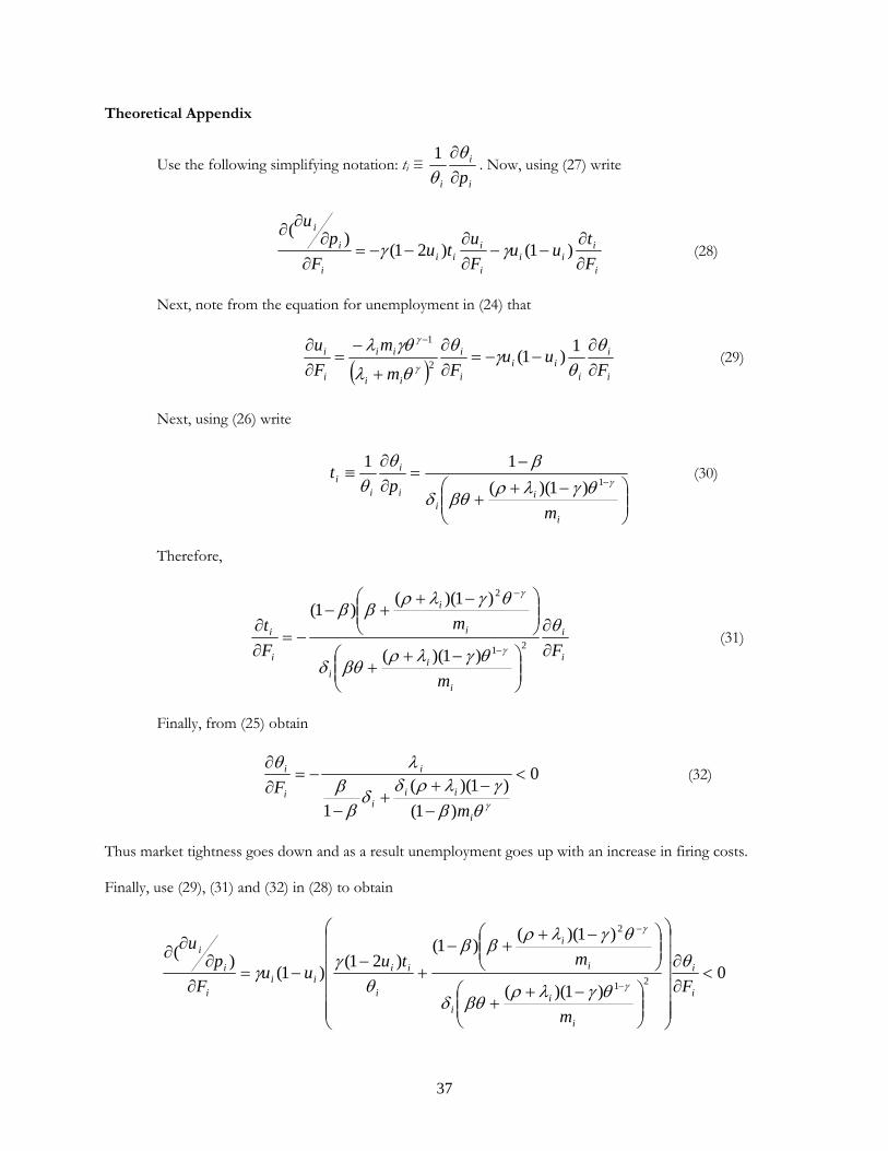
37

Theoretical Appendix

Use the following simplifying notation: ti ≡ i

i

i p

1

. Now, using (27) write

i

iii

i

iii

i

i

i

F

tuu

F

utu

F

pu

)1()21(

)( (28)

Next, note from the equation for unemployment in (24) that

i

i

iii

i

i

ii

ii

i

i

Fuu

Fm

m

F

u

1)1(

2

1

(29)

Next, using (26) write

i

ii

i

i

ii

m

pt

1)1)((

11 (30)

Therefore,

i

i

i

ii

i

i

i

i

F

m

m

F

t

21

2

)1)((

)1)(()1(

(31)

Finally, from (25) obtain

0

)1(

)1)((

1

i

iii

i

i

i

mF

(32)

Thus market tightness goes down and as a result unemployment goes up with an increase in firing costs.

Finally, use (29), (31) and (32) in (28) to obtain

0)1)((

)1)(()1(

)21()1(

)(

21

2

i

i

i

ii

i

i

i

iiii

i

i

i

F

m

mtuuu

F

pu