Trade intensity and business cycle synchronization: Are developing countries any different?

m/locate/econbase
Journal of International Economics 71 (2007) 2–21
www.elsevier.co

Trade intensity and business cycle synchronization:Are developing countries any different?☆

César Calderón a, Alberto Chong b,⁎, Ernesto Stein b

a The World Bank, 1818 H Street NW, Washington DC 20433, USAb Inter-American Development Bank, 1300 New York Avenue NW, Washington DC 20577, USA

Received 19 February 2003; received in revised form 31 May 2006; accepted 20 June 2006

Abstract

Trade intensity increases the business cycle co-movement among industrial countries. Using annualinformation for 147 countries for the period 1960–99 we find that the impact of trade intensity on businesscycle correlation among developing countries is positive and significant, but substantially smaller than thatamong industrial countries. Our findings suggest that differences in the responsiveness of cyclesynchronization to trade integration between industrial and developing countries are explained bydifferences in the patterns of specialization and bilateral trade.© 2006 Elsevier B.V. All rights reserved.

Keywords: Bilateral trade; Cycle synchronization; LDCs; Intra-industry trade; Integration

JEL classification: E32; F15; O10

1. Introduction

The recent creation of the European Monetary Union (EMU) has renewed the interest in theeconomics of currency unions. While such unions may foster trade flows among their members,

☆ Comments by Alejandro Micco, Klaus Schmidt-Hebbel, anonymous referees, the editor, Enrique Mendoza, andseminar participants at the North American Econometric Society Summer Meetings are greatly appreciated. VirgilioGaldo, Gianmarco Leon, and Josefina Posadas provided excellent research assistance. The ideas expressed in this paper arethose of the authors, and do not necessarily reflect those of the World Bank or the Inter-American Development Bank ortheir corresponding executive directors. The standard disclaimer applies.⁎ Corresponding author. Research Department, Stop B-900, Research Department, Inter-American Development Bank,

1300 New York Ave., NW, Washington, DC 20577, USA. Tel.: +1 202 623 1536; fax: +1 202 623 2481.E-mail addresses: [email protected] (C. Calderón), [email protected] (A. Chong), [email protected]

(E. Stein).

0022-1996/$ - see front matter © 2006 Elsevier B.V. All rights reserved.doi:10.1016/j.jinteco.2006.06.001

mailto:[email protected]



http://dx.doi.org/10.1016/j.jinteco.2006.06.001

3C. Calderón et al. / Journal of International Economics 71 (2007) 2–21

the sacrifice of an independent monetary policy may also pose important costs, in particular whenthe correlation between the business cycles of the different member countries is relatively low.But what factors determine such correlation? In the last several years, a number of scholars havefocused on the role of one particular such factor, namely the degree of trade integration. As arguedby Frankel and Rose (1997, 1998), if currency unions create trade, and trade increases cyclecorrelation, perhaps countries should not be so concerned with ex-ante lack of business cyclecorrelation when deciding whether to enter into a currency union.

Empirical studies for the case of industrial countries (Frankel and Rose, 1997, 1998; Fatás,1997; Clark and van Wincoop, 2001) provide evidence that higher trade integration does in factlead to more closely correlated business cycles. But are the lessons derived from the experience ofindustrial countries useful to help guide policy decisions in developing countries? We argue thatthere are reasons to believe that the link between these variables may be weaker amongdeveloping countries. The response of business cycle synchronization to trade integration maydepend on variables such as differences in structures of production among country pairs(Krugman, 1991), and the extent of intra-industry trade (Fidrmuc, 2002; Gruben et al., 2002;Imbs, 2004). Since these factors may differ for different types of country pairs, the impact tradeintegration on business cycle correlation may be different as well.

According to the literature, the impact of trade integration on business cycle correlation couldgo either way (Frankel and Rose, 1998). On the one hand, if the demand channel is the dominantforce driving business cycles, we expect trade integration to increase cycle correlation. Forinstance, positive output shocks in a country might increase its demand for foreign goods. Theimpact of this shock on the cycle of the country's trading partners should depend on the depth ofthe trade links with each of the partners. On the other hand, if industry-specific shocks are thedominant force in explaining cyclical output, the relationship would be negative if increasingspecialization in production leads to inter-industry trade (as usually observed in developingcountries). In this case, trade integration leads to specialization in different industries, which inturn leads to asymmetric effects of industry-specific shocks. In contrast, if intra-industry tradeprevails (as observed in industrial countries), specialization does not necessarily lead toasymmetric effects of industry-specific shocks, since the pattern of specialization occurs mainlywithin industries. In summary, the total effect of trade intensity on cycle correlation istheoretically ambiguous and poses a question that could only be solved empirically. However, theimportant differences in the pattern of trade and specialization among country pairs of differenttype suggest that the impact of trade integration on cycle correlation among developing countriesmay differ substantially from that among industrial countries.

Our paper extends and complements the study of Frankel and Rose (1998) in two dimensions:first, we analyze the impact of trade integration on business cycle correlation not only amongindustrial countries but also among developing countries, as well as among “mixed” (industrial-developing) country pairs. By working with a sample of 147 industrial and developing countries,we are able to test whether the links between trade intensity and business cycle correlation aredifferent depending on the nature of the countries involved. We expect the impact to differ acrossgroups of countries, due to their different patterns of trade and specialization (i.e., inter- vs. intra-industry trade patterns). Our prior is that trade intensity should have a positive effect on cyclicaloutput correlation among industrial countries, and a smaller (and ambiguous) effect among othercountry pairs. Following Frankel and Rose (1998), in studying the effects of trade intensity oncycle correlation we take into account the fact that trade intensity itself may be endogenous.

Second, we study the extent to which differences in the response of output correlation to highertrade integration among different groups of country pairs can be attributed to differences in the

4 C. Calderón et al. / Journal of International Economics 71 (2007) 2–21

structures of production and the nature of bilateral trade patterns. In analyzing the role played bythese factors, our prior is that the impact of bilateral trade intensity on output correlationwill be largerfor country pairs with similar economic structures and with a larger share of intra-industry trade.

Among our main findings, we have that:

(1) On average, higher trade integration leads to higher business cycle synchronization. Thisresult is robust to changes in the measure of bilateral trade intensity, to the detrendingtechniques used to compute cyclical output, or the estimation method (OLS or IV).

(2) Our coefficient estimates suggest that the correlation between cyclical output increasesfrom a starting mean of 0.05 to 0.085 when the bilateral trade intensity increases by onestandard deviation.

(3) The impact of trade intensity on business cycle correlation for industrial countries issignificantly higher than the one for the sample of developing countries and the sample of“mixed” country pairs. In particular, a one standard deviation increase in our coefficient ofbilateral trade leads to a surge in our business cycle correlation from a starting mean of: (a)0.25 to 0.33 for industrial countries, (b) 0.075 to 0.077 for our sample of mixed countrypairs, and (c) 0.031 to 0.052 for our sample of developing countries. Note that result in (a) issimilar to the one found by Frankel and Rose (1998) although we are working with a largersample and different time period.

(4) We find robust evidence of a negative interaction effect between trade integration and anindex of asymmetries in the structure of production (which we use as a proxy for the extentof inter-industry trade). As expected, the impact of trade intensity on cycle correlation islarger when countries have similar production structures.

(5) We also find a positive interaction between trade integration and the Grubel-Lloyd index ofintra-industry trade. This result implies that the impact of trade intensity on cyclecorrelation is larger for country pairs with a higher share of intra-industry trade.

(6) We address the issue of how much of the difference in the coefficient estimates betweenindustrial and developing country pairs is attributed to either asymmetries or intra-industrypatterns. Specifically, we find that asymmetries in the structure of production (orspecialization) explains approximately 40% of the differences in the sensitivity of cyclecorrelation to trade intensity between industrial and developing country pair groups, while30% of such differences may be attributed to intra-industry trade patterns.

The rest of the paper is organized as follows. Section 2 provides some theoretical insightsregarding the relationship between trade integration and the synchronization of business cycles.Section 3 discusses the data and presents the econometric methodology used in our empiricalevaluation. Section 4 discusses the main empirical results and relevant extensions. Finally,Section 5 concludes.

2. Some theoretical insights

In order to understand the different channels through which trade intensity can impact businesscycle synchronization, we use Stockman's (1988) decomposition of growth in country i at time t(dlnyit) into the weighted average of industry-specific shocks (ξkit) – with the weights ωki beingapproximated by the share of sector k's output in total output – and an aggregate shock (ηit).

We assume that {ξkit} is distributed independently of each other across both sector and time,with sectoral variance σk

2; industry shocks are similar across countries (ξkit =ξkjt), and have the


same variance σk2; {ηit} is distributed independently over time; and finally {ξkit} and {ηit} are

independent from each other. Hence, the covariance between the growth rates of countries i and j,σ(yi, yj), is:

rðyi;yjÞ ¼ r2kXk

xkixkj þ rðgi;gjÞ ð1Þ

where σ(ηi,ηj) is the covariance between country-specific aggregate shocks.According to the literature, the impact of greater trade integration on business cycle

synchronization is theoretically ambiguous. Standard trade theory (Heckscher-Ohlin paradigm)predicts that openness to trade would lead to an increasing specialization in production alongindustry lines, and inter-industry patterns of international trade (as typically observed amongdeveloping countries). If business cycles are dominated by industry-specific shocks, ξkit, wewould expect that higher trade integration, by bringing about deeper specialization, would lead todecreasing business cycle correlations (i.e., we expect a negative correlation between ωki andωkj). Kalemli-Ozcan, Sorensen and Yosha (2001) find another mechanism that will render anegative correlation between trade integration and business cycle correlations. With higherintegration in both international financial markets and goods markets, countries should be able toinsure against asymmetric shocks through diversification of ownership and can afford to have aspecialized production structure. In this case, better opportunities for income diversificationinduce higher specialization in production, which are associated with more asymmetric businesscycles.

On the other hand, if patterns of specialization in production and international trade aredominated by intra-industry trade (as frequently observed among industrial countries), deepertrade links will not necessarily result in deeper specialization along industry lines, as predicted bystandard trade theory. In this case, then, industry specific shocks will not necessarily affectdifferent countries more asymmetrically as they become more integrated (see Krugman, 1993). Interms of the model, deeper trade integration does not necessarily lead to a negative correlationbetween ωki and ωkj. Consistent with the intra-industry perspective, it has been shown that anincreasing amount of trade is vertical or fragmented and that more of this “back-and-forth” trademight lead to a greater response of the business cycle correlations to higher trade integration(Kose and Yi, 2001).

Finally, higher integration is likely to have an impact on the cycle synchronization by raisingthe covariance between country-specific aggregate shocks, σ(ηi,ηj). First, spillover effects fromaggregate demand shocks might increase this covariance. In this case, surges in income in onecountry might lead to higher demand for both foreign and domestic goods. This effect might beeven stronger if trade integration leads to more coordinated policy shocks (Frankel and Rose,1998).1 Second, higher trade integration might lead to a more rapid spread of productivity shocksthrough a more rapid diffusion of knowledge and technology (Coe and Helpman, 1995) or viainward FDI and technology sourcing (Lichtenberg and van Pottelsberghe, 1998).

In sum, the relationship between trade integration and business-cycle synchrony is theore-tically ambiguous. While the impact is positive if country-specific aggregate shocks dominatebusiness cycles, the effect of trade integration is not clear if industry-specific shocks are the mainsource of business cycle. In the latter case, the nature of the relationship between trade integrationand cyclical output correlations depend on the patterns of specialization in production once the

1 In the presence of fiscal consolidation or more coordinated monetary policies, the impact of spillovers from aggregatedemand is even larger.


economy is open to international markets. Given the observed patterns of specialization in theworld economy, we expect a positive correlation between trade integration and business cyclecorrelations among industrial countries, and a more ambiguous relationship (i.e., positive andsmaller than among industrial countries, and in some cases negative) among industrial-deve-loping country pairs and among developing countries.

3. Data and methodology

3.1. The data

The core of our empirical analysis lies on themeasurement of both bilateral trade intensity and thebilateral correlations of real economic activity. Our dependent variable is the degree of business cyclesynchronization between countries i and j at period τ (of length T). To measure this variable, wefollow Frankel and Rose (1997, 1998) and compute the correlation between the cyclical compo-nents of output for countries i and j. Our measure of real output is the (log of) real GDP in localcurrency at constant prices, taken from the World Bank's World Development Indicators. Thecyclical component of output in country i (yi

C) is obtained using different trend-cycle decompositiontechniques.

Given the lack of consensus about optimal detrending techniques and for robustness purposes,we use four different procedures to decompose real output into trend and cycle: (a) the quadratictrend model, (b) first differences, (c) the Hodrick-Prescott (HP) filter, and (d) the band-pass filter.For the discussion of our results the preferred detrending technique is the band-pass filterproposed by Baxter and King (1999). Unlike other trend-cycle decomposition techniques, thisfilter takes into account the statistical features of the business cycle.2

We apply the different filters on the output series over the entire sample period, 1960–99. Oncewe compute this cyclical component, we calculate the correlation between detrended output incountries i and j over the entire period (for our cross-section analysis), and correlation coefficientsfor each decade (for our panel data analysis). According to this measure, higher output correlationbetween countries i and j implies a higher degree of business cycle synchronization.

The bilateral intensity of international trade between countries i and j in period τ (of length T)is approximated with the following measures:

TFi;j;s ¼ ln

1T

Xt

1þ fi;j;tFi;t þ Fj;t

!and TY

i;j;s ¼ ln1T

Xt

1þ fi;j;tYi;t þ Yj;t

!ð2Þ

where fi,j,t denotes the amount of bilateral trade flows (exports and imports in US dollars) betweencountries i and j. Also, Fkt represents total (multilateral) trade –exports and imports – of country k(with k= i,j) in period t (also in US dollars). Note that the numerator in (2) is (1+ fi,j,τ) in order todeal with zero-trade observations, which would otherwise be dropped by taking logs. This is not aproblem in studies which focus on industrial countries, since in that case bilateral trade flows arenon-zero. In our case, nearly 20% of the observations in our panel data set which includes 147countries have zero trade flows. In order to prevent the loss of these observations, which may

2 Note that although we used the band-pass filter as our preferred detrending technique, the results that we will presentin Section 4 are robust to any of the four trend-cycle decomposition techniques used in this paper. Results are availablefrom the authors upon request.


contain important information, we add one to the bilateral trade flows, which is one of thestandard ways to deal with this problem in the context of gravity models of bilateral trade.3

In Eq. (2), we compute Ti,j,τF as the ratio of bilateral trade flows between countries i and j

divided by the sum total trade flows (exports and imports) of countries i and j. Our secondmeasure, Ti,j,τ

Y , is the ratio of bilateral trade flows between countries i and j to output in bothcountries (Yi,t and Yj,t, respectively). The bilateral trade data are taken from the InternationalMonetary Fund's Direction of Trade Statistics, whereas nominal and real GDP data are taken fromthe World Bank's World Development Indicators. We gather annual data for the 1960–99 periodon bilateral trade flows for the 147 countries in our sample (see Appendix I for our list ofcountries), and we used exports FOB and imports CIF in order to construct the measures specifiedin Eq. (2).4

A typical problem of bilateral trade data is that export flows from country i to country j are notnecessarily equal to import flows of country j from country i. In this case, we have always reliedon the data reported by the country with higher income in the country pair. Since it is not clearwhether it is more appropriate to build the measures of trade intensity normalizing by trade ortotal output, we conduct our econometric tests using both. Hence, we compute averages over theannual data for the 1960–99 period (for our cross-sectional analysis) and for each decade (for ourpanel data analysis). Our discussion of the results will mainly focus on the bilateral trade figuresnormalized by output since it captures with more accuracy the effective degree of integrationbetween two countries.5

In order to extend and complement the evidence presented by Frankel and Rose (1998), wealso analyze the impact of intra-industry trade intensity on business cycle synchronization byconstructing the Grubel and Lloyd (1975) measure of intra-industry trade between countries i andj, GLIi,j:

GLIi;j ¼ 1−Xk

jxki;j−mki;jj=Xk

ðxki;j þ mki;jÞ

!ð3Þ

where xi,jk and mi,j

k are exports from country i to country j and imports from country i to country j,respectively, and k represents an index over industries. Our data on intra-industry trade have beenobtained from the World Trade Analyzer assembled by Statistics Canada compiled anddocumented by Feenstra (2000). Here, we use the SITC 4-digit level bilateral exports and importsfor our sample of 147 countries. For a more detailed description of the data, see Feenstra (2000).We should note that we only have annual data for our Grubel-Lloyd measure of intra-industrytrade for the 1980–98 period. Hence, we compute averages for the almost 20 years of data for ourcross-section sample and decade averages for our panel data sample.

Finally, to test the robustness of coefficient estimate of trade intensity to the inclusion ofpossible omitted variables, we include a proxy of differences in the economic structures of thedifferent economies. Similarities in the structure of production imply that industry-specificshocks tend to have similar effects on aggregate fluctuations across national borders. Evidence

3 See, for example, Eichengreen and Irwin (1998). We should note, however, that dropping the zero observations (i.e.,not adding unity to the bilateral trade flow) does not change the results in any significant way.4 Although there were data for imports FOB on the IMF's Direction of Trade Statistics, the data availability were more

limited. That is, they represent at most 20% of the coverage with imports CIF.5 For example, the share of bilateral trade to total trade between countries i and j could be very high (say, for a pair of

remote countries). However, both could have a small external sector and, therefore, the share of bilateral trade to theiroutputs could be very small.


shows that these shocks will generate higher degree of business cycle synchronization amongregions with similar production structures rather than among regions with asymmetric structures(Imbs, 2001; Kalemli-Ozcan et al., 2001; Imbs, 2004).

Similarities in the structure of production are approximated using the absolute value indexsuggested by Krugman (1991). Letting Sk,i and Sk,j denote the GDP shares for industry k incountries i and j (k=1, 2,…, N industries), we compute an index of asymmetries in structures or

production ASPi,j,τ (averaged over period τ of length T) as ASPi;j;s ¼ 1T

Pt

PNk¼1

jSki−Skjj. Thehigher the value of ASPi,j,τ, the greater the difference in industry shares between countries i and jand, therefore, the greater the differences in structures or production. We measure industryspecialization using the 9-sector classification from the 1-digit level ISIC code and the data wereobtained from the World Bank and UNIDO. The ASP index is computed over the 1960–99period, however, due to the lack of availability for some countries, the panel data information onthis variable is not balanced — especially for developing countries.

3.2. Empirical strategy

We have collected annual data for 147 countries over the 1960–99 period on both real GDPand bilateral trade. Using the annual data for the 1960–99 period, we compute the cyclicalcomponent of real output. Then we compute the (detrended) output correlation between countriesi and j over period τ of length T. We analyze two samples: First, a cross-sectional sample ofcountry pairs for the period 1960–99. There, we compute the correlation coefficient over thewhole sample period and we averaged our annual data on bilateral trade intensity over the40 years of data. Second, we analyze a panel data sample where we split our 40 years of data intofour equally sized parts: 1960–69, 1970–79, 1980–89, and 1990–99. There, we compute theoutput correlations and average the annual data on bilateral trade over each of the decades.

3.2.1. The regression frameworkIn order to test the impact of trade integration (approximated by coefficients of bilateral trade

intensity) on business cycle synchronization (measured by the correlation between cyclicaloutputs), we run the following panel regression equation:

qðyCi ;yCj Þs ¼ ai;j þ bs þ gTKi;j;s þ uASPi;j;s þ ui;j;s ð4Þ

where ρ(yiC,yj

C) denotes the business cycle correlation between countries i and j over time periodτ (of length T=10 years), Ti,j,τ

K is the average bilateral trade intensity between countries i and jover time period τ, either normalized by trade (K=F) or output (K=Y), and ASPi,j,τ is the measureof industry specialization. In addition, αi,j represent country pair-specific effects, while βτ aretime effects which are proxied by decade dummies.

There are two reasons why we prefer this specification including country pair fixed effects. First,including country pair fixed effects allows us to control for all the time-invariant, country pair-specific variables which may have an impact on output correlation. For example, a pair of countriesmay be very proximate and subject to common natural disasters such as hurricanes or floods.Alternatively, both countries in the pair may have a very high degree of trade intensity with the samethird country, and through this channel their outputs may be highly correlated. These factors, as wellas other omitted variables, will be captured by the country pair fixed effect. But perhaps moreimportantly, including the country pair fixed effects leads us to focus on the time series dimension


and, thus, on the right policy question. What we want to know is what happens to output correlationbetween a pair of countries when bilateral trade intensity among them increases. This is not exactlythe same as asking whether country pairs with higher bilateral trade intensity have higher outputcorrelation than other country pairs, which is the question answered by the cross-section regressions.As Glick and Rose (2002) have argued convincingly in their analysis of the impact of monetaryunions on trade, the former – and not the latter – is the right policy question.

Our main interest lies on the sign and the magnitude of the slope coefficient γ. If industryshocks are the dominant source of business cycles and openness to trade leads to completespecialization (as Heckscher-Ohlin would predict), we would expect γ to be negative. On theother hand, if industry shocks lead to vertical specialization (and, therefore, more intra-industrytrade), or if global shocks dominate economic fluctuations then we would expect γ to be positive.

A problem with Eq. (4) is that, as discussed earlier, trade intensity itself may be endogenous.Higher output correlation could encourage countries to become members of a currency union,which in turn could lead to increased trade intensity (Frankel and Rose, 1998, 2002; Rose andEngel, 2002). Alternatively, both of our variables of interest, namely output correlation and tradeintensity, could be explained by a third one, such as currency union, which at the same timereduces transactions costs in trade flows, and links the macroeconomic policies of their members.Hence, countries joining a currency union might exhibit a positive correlation between tradeintegration and business cycle synchronization. In this context, running an OLS regression for Eq.(4) would yield biased and inconsistent estimates for γ. Given the problems mentioned above, weneed instruments for the bilateral trade intensity in order to estimate γ consistently. FollowingFrankel and Romer (1999), we use the gravity model of bilateral trade to motivate our choice ofinstrumental variables. Based on Wei (1996) and Deardorff (1998), we specify the followingregression for bilateral trade:

TKi;j ¼ b0 þ b1lndij þ b2Bij þ b3lnREMi þ b4lnREMj þ Z Vhþ eij

where Ti,jK is our measure of bilateral trade flows country i to country j either normalized by trade

(K=F) or output (K=Y), dij is the distance between countries i and j (in logs), and Bij is a dummyvariable equal to one for countries that share a common border. We expect that bilateral tradebetween countries i and j will increase if their outputs increase, if they are closer in distance, and ifthey share a common border. Furthermore, we include an indicator of geographical remoteness forcountries i and j that measures how far each country lies from alternative trading partners —REMi and REMj, respectively.

6

Finally, the matrix Z comprises other variables that are used in the empirical literature of thegravity equation model of trade. Here, we include other standard controls in this literature such asthe initial population and area in countries i and j, number of islands and landlocked countries inthe (i,j) country pair, dummies for common geographical region, common language, commoncolonial origin, and common main trading partner.

4. Empirical assessment

In this section, we present our empirical assessment on the relationship between tradeintegration and business cycle synchronization for the sample of all country pairs. As we stated in

6 For a given country pair (i,j), the remoteness of country i is defined as REMi ¼P

mpjðym=ywÞdim. Stein and Weinhold(1998) argue that this measure complies with several desirable properties for a measure of remoteness.


Section 3, we have annual data on output and bilateral trade for 147 countries over the 1960–99period. To measure our dependent variable, we compute the cyclical component of real GDP overour sample period using different detrending techniques, then we compute the business cyclecorrelation between countries i and j over a given span of time. In this case, we split the 1960–99period into four equally sized subperiods, and we are able to compute a total of 33,676 bilateraloutput correlations 6232 for the 1960s, 7753 for the 1970s, 10127 for the 1980s, and 9564 for the1990s). Likewise, our annual data on bilateral trade intensity is averaged over each decade to becompatible with our regression framework.

4.1. Descriptive statistics

In Table 1 we present averages and standard deviations of the variables involved in our analysis:cycle correlation, trade intensity and asymmetries in production structures. In panel I of Table 1 weshow averages of our measures of business cycle synchronization. We find that the correlation ofoutput cycles for all country pairs over the period 1960–99 is 0.05. On the other hand, outputs aremore correlated among industrial country pairs than any other group of country pairs regardless ofthe detrending technique used. For instance, band-pass filter estimates show that output correlationis 0.254 for industrial country pairs, 0.075 for mixed industrial-developing country pairs, and0.031 for developing country pairs. Note that when comparing output correlation measures, wefind that the ones obtained using the quadratic trend have a small degree of association with theones obtained with other filters (between 0.37 and 0.41). On the other hand, output correlations

Table 1Trade intensity and cycle synchronization: summary statistics 1/

Detrended output correlation using: All Countrypairs

Selected country pairs

(IND, IND) (IND, DEV) (DEV, DEV)

I. Business cycle synchronization–Quadratic trend (QT) 0.065 (0.56) 0.260 (0.56) 0.069 (0.56) 0.055 (0.56)–First differences (1D) 0.037 (0.37) 0.226 (0.39) 0.058 (0.37) 0.020 (0.37)–Hodrick–Prescott (HP) 0.059 (0.39) 0.252 (0.39) 0.086 (0.39) 0.039 (0.38)–Band-pass filter (BP) 0.050 (0.38) 0.254 (0.37) 0.075 (0.38) 0.031 (0.37)

II. Bilateral trade intensity 2/2.1. Ratios–Normalized by trade −9.12 (2.49) −5.72 (1.42) −8.73 (2.23) −9.67 (2.47)–Normalized by output −9.66 (2.36) −6.58 (1.47) −9.37 (2.12) −10.09 (2.38)

2.2. Instrumented ratios (IV) 3/–Normalized by trade −8.84 (1.60) −6.46 (1.54) −9.04 (1.41) −8.92 (1.57)–Normalized by output −9.36 (1.41) −7.33 (1.46) −9.54 (1.23) −9.41 (1.39)

III. Intra-industry trade and asymmetriesGrubel-Lloyd index of intra-industry trade 4/ 0.022 (0.07) 0.208 (0.17) 0.029 (0.06) 0.009 (0.04)Asymmetries in structures of production (9 Sector) 5/ 0.399 (0.22) 0.133 (0.07) 0.446 (0.23) 0.393 (0.21)

Full sample of country pairs, 1960–99.1/ In this table, we report the mean of the variable. The number in parentheses below the mean is the standard deviation. Onthe other hand, we denote (IND,IND) as the country pairs of industrial countries, (DEV,DEV) are the country pairs ofdeveloping countries, and (IND,DEV) represent mixed country pairs of industrial and developing countries.2/ The coefficient of bilateral trade intensity is computed according to Eq. (2), expressed in logs.3/ Instrumented averages are the adjusted values of the first stage regression presented in Table 3.4/ The Grubel and Lloyd (1975) measure of intra-industry trade computed according to Eq. (3).5/ The 9-sector index of asymmetries in the structures of production takes into account the asymmetries betweencountries.


obtained with the other filters are highly correlated among them. Specifically, the first-differencedoutput correlations has a degree of association of 0.77 and 0.78 with the Hodrick-Prescott andband-pass filtered output correlations; while the latter two measures of output synchronizationhave a correlation of 0.94. From now on, our discussion will be centered on the results using theband-pass-filtered output correlations for the reasons mentioned in Section 3.1.

In addition to more correlated outputs, industrial country pairs, not surprisingly, also exhibitmuch higher bilateral trade intensities than country pairs of mixed industrial-developing countriesor country pairs of developing economies, whether these trade intensities are normalized byoutput or by trade (see panel II of Table 1).7 They also exhibit more similar production structures,with an index of production asymmetries that is about one third of that corresponding to the othertwo country pair groups, and a much higher degree of intra-industry trade (see panel III ofTable 1).

4.2. Regression analysis

Before moving on to our regression analysis, we present simple correlations between ourmeasures of output synchronization and bilateral trade intensity for each of the country pairgroups, as well as the sample as a whole. The idea is to provide a rough first look at the mainquestion addressed in this paper: is the link between output correlation and bilateral trade intensitydifferent for different groups of countries? Whether we focus on the cross-section data, or thepooled panel data, the answer to our question seems to be a resounding yes. In the case of thepooled panel data, the correlation between our two variables of interest is about five times largerin the case of industrial countries (0.269), compared to the other two groups of country pairs(0.044 and 0.052 for mixed and developing country pairs when normalizing by output,respectively). The results suggest that, while countries with higher trade linkages tend to displaymore synchronized business cycles for all groups of countries, the association is much stronger inthe case of industrial countries.

While the results of the simple correlations support our priors, they are merely suggestive.First, the simple correlations present evidence of the association between our variables of interest,but association does not necessarily imply causality. If the arguments regarding endogenousoptimal currency areas are going to carry some weight, association is not enough, it is necessary toshow that higher trade intensity leads to higher output correlation. Second, in the simple exerciseconducted above we have not controlled for other factors that may explain the degree of businesscycle correlation such as, for example, the degree to which the production structures are similaracross countries. These issues are addressed next, when we present the results of our regressionanalysis. The discussion will focus on the estimates of our parameter of interest γ in Eq. (4). Afterpresenting results using different estimation techniques for the sample of countries as a whole(Section 4.2.1), in Section 4.2.2 we will come back to our main question: are developing countriesany different? Finally, Section 4.2.3 will explore the channels for these different results across

7 Note that the unit of increase that we will use in our economic interpretation is a one standard deviation which isconventionally used in most studies in this strand of the literature (e.g., Frankel and Rose, 1998). As we observe, thestandard deviation computed for the trade intensity indicator in the regression sample yields the following: (a) using theactual values of trade intensity ratios, we have that trade ratios among developing countries are more volatile than amongindustrial economies (2.4 vs. 1.5, when normalized by trade). (b) Using the instrumented values of the trade intensityratios (after adjusting for scale and geographic variables), the differences are smaller and the volatility of the adjustedratio for industrial country pairs (1.46) is slightly larger than the volatility of trade among developing countries (1.39).


country pair groups, emphasizing the role of production asymmetries, as well as the intra- or inter-industry nature of the countries' trade.

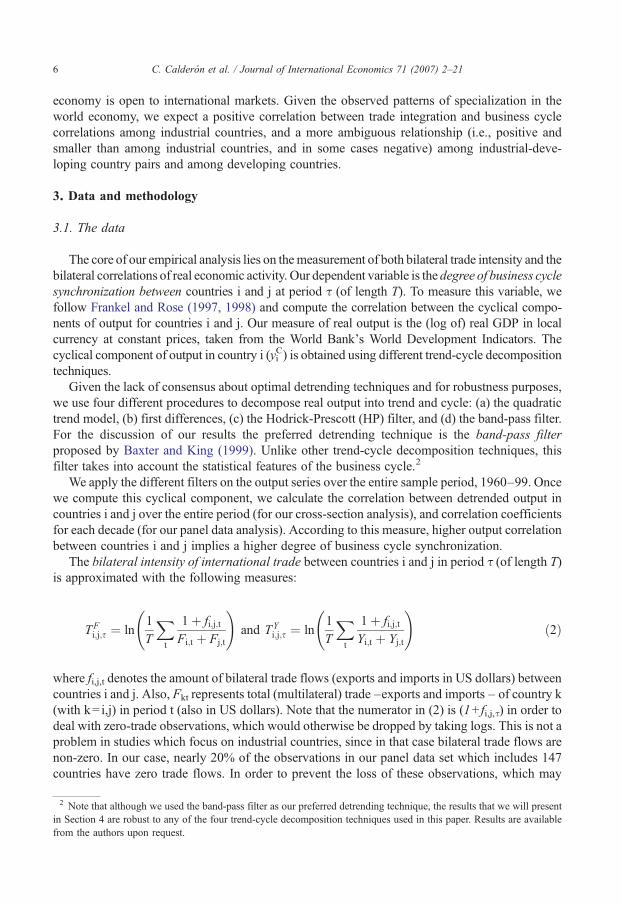
4.2.1. All country pairsIn Table 2, we start by presenting our OLS estimates of Eq. (4) for the sample of countries as a

whole. The regressions in the last two columns include a control for the index of productionasymmetries which, as expected, is negative and significant (i.e., more asymmetries implies alower output correlation). This result is similar to the one found by Imbs (2004), where patterns ofspecialization have a significant effect on cycle correlation. We want to focus our discussion onthe lower panel of the Table, where we work with panel data, and include country pair fixedeffects.

Table 2 suggests that, regardless of the model we use, there is a positive and significantrelationship between bilateral trade intensity and output correlation. The panel coefficient

Table 2Trade intensity and cycle synchronization: regression analysis

Variable Cross-section Panel data 1/

Baseline Augmented Baseline Augmented

I. Least squares1.1 Bilateral trade normalized by total tradeBilateral trade intensity 5.49E–03⁎⁎ 4.82E-03⁎⁎ 0.0142⁎⁎ 0.0123⁎⁎

(10.03) (8.50) (11.85) (8.98)Asymmetries in the structure of production … −0.0490⁎⁎ … −0.0168

4.45 (1.23)Number of observation 7993 7470 17721 14109

1.2 Bilateral trade normalized by total outputBilateral trade intensity 5.50E–03⁎⁎ 4.86E–03⁎⁎ 0.0138⁎⁎ 0.0126⁎⁎

(10.54) (8.90) (11.74) (9.15)Asymmetries in the structure of production … −0.0511⁎⁎ … −0.0260⁎⁎

(4.74) (1.96)Number of observations 8567 7781 19511 14664

II. Instrumental variables 1/ 2/2.1 Bilateral trade normalized by total tradeBilateral trade intensity 7.41E–03⁎⁎ 4.73E–03⁎⁎ 0.022⁎⁎ 0.015⁎⁎



2.2 Bilateral trade normalized by total outputBilateral trade intensity 8.17E–03⁎⁎ 6.93E–03⁎⁎ 0.025⁎⁎ 0.019⁎⁎



Full sample of country pairs, 1960–99.Numbers in parenthesis below the estimated coefficients represent their t-statistics. ⁎ (⁎⁎) Reflects significance at 10 (5)%.1/ The measures of bilateral trade intensity are instrumented with the distance between countries j and k, a dummy forcommon border, remoteness of countries j and k, population, and area in both countries, number of islands and landlockedcountries in the pair, and dummies for common geographical region, language, and colonial origin, and common tradingpartner. Note that all panel data regressions include decade dummies. 2/ See the results of the first stage regression inTable 3.


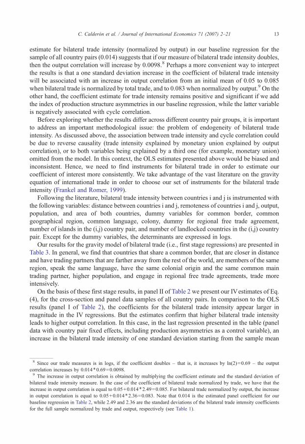
estimate for bilateral trade intensity (normalized by output) in our baseline regression for thesample of all country pairs (0.014) suggests that if our measure of bilateral trade intensity doubles,then the output correlation will increase by 0.0098.8 Perhaps a more convenient way to interpretthe results is that a one standard deviation increase in the coefficient of bilateral trade intensitywill be associated with an increase in output correlation from an initial mean of 0.05 to 0.085when bilateral trade is normalized by total trade, and to 0.083 when normalized by output.9 On theother hand, the coefficient estimate for trade intensity remains positive and significant if we addthe index of production structure asymmetries in our baseline regression, while the latter variableis negatively associated with cycle correlation.

Before exploring whether the results differ across different country pair groups, it is importantto address an important methodological issue: the problem of endogeneity of bilateral tradeintensity. As discussed above, the association between trade intensity and cycle correlation couldbe due to reverse causality (trade intensity explained by monetary union explained by outputcorrelation), or to both variables being explained by a third one (for example, monetary union)omitted from the model. In this context, the OLS estimates presented above would be biased andinconsistent. Hence, we need to find instruments for bilateral trade in order to estimate ourcoefficient of interest more consistently. We take advantage of the vast literature on the gravityequation of international trade in order to choose our set of instruments for the bilateral tradeintensity (Frankel and Romer, 1999).

Following the literature, bilateral trade intensity between countries i and j is instrumented withthe following variables: distance between countries i and j, remoteness of countries i and j, output,population, and area of both countries, dummy variables for common border, commongeographical region, common language, colony, dummy for regional free trade agreement,number of islands in the (i,j) country pair, and number of landlocked countries in the (i,j) countrypair. Except for the dummy variables, the determinants are expressed in logs.

Our results for the gravity model of bilateral trade (i.e., first stage regressions) are presented inTable 3. In general, we find that countries that share a common border, that are closer in distanceand have trading partners that are farther away from the rest of the world, are members of the sameregion, speak the same language, have the same colonial origin and the same common maintrading partner, higher population, and engage in regional free trade agreements, trade moreintensively.

On the basis of these first stage results, in panel II of Table 2 we present our IVestimates of Eq.(4), for the cross-section and panel data samples of all country pairs. In comparison to the OLSresults (panel I of Table 2), the coefficients for the bilateral trade intensity appear larger inmagnitude in the IV regressions. But the estimates confirm that higher bilateral trade intensityleads to higher output correlation. In this case, in the last regression presented in the table (paneldata with country pair fixed effects, including production asymmetries as a control variable), anincrease in the bilateral trade intensity of one standard deviation starting from the sample mean

8 Since our trade measures is in logs, if the coefficient doubles – that is, it increases by ln(2)=0.69 – the outputcorrelation increases by 0.014⁎0.69=0.0098.9 The increase in output correlation is obtained by multiplying the coefficient estimate and the standard deviation of

bilateral trade intensity measure. In the case of the coefficient of bilateral trade normalized by trade, we have that theincrease in output correlation is equal to 0.05+0.014⁎2.49=0.085. For bilateral trade normalized by output, the increasein output correlation is equal to 0.05+0.014⁎2.36=0.083. Note that 0.014 is the estimated panel coefficient for ourbaseline regression in Table 2, while 2.49 and 2.36 are the standard deviations of the bilateral trade intensity coefficientsfor the full sample normalized by trade and output, respectively (see Table 1).

Table 3First stage regressions: gravity equations dependent variable: bilateral trade intensity between countries j and k

Variable Normalized by total trade Normalized by total output

Cross-section Panel data Cross-section Panel data

Constant −20.87⁎⁎ −9.12⁎⁎ −13.84⁎⁎ −4.45⁎⁎(23.37) (6.41) (14.83) (3.25)

Distance (in logs) −2.02⁎⁎ −0.99⁎⁎ −2.07⁎⁎ −1.04⁎⁎(29.56) (30.03) (29.55) (33.88)

Border dummy −0.04 0.98⁎⁎ −0.04 0.81⁎⁎

(0.17) (9.85) (0.15) (8.83)Remoteness country j 0.79⁎⁎ −2.28⁎⁎ 1.94⁎⁎ −2.21⁎⁎

(1.95) (25.37) (4.57) (25.40)Remoteness country k −0.91⁎⁎ −1.16⁎⁎ 1.10⁎⁎ −0.80⁎⁎

(2.23) (12.92) (2.68) (9.22)Population country j (logs) 1.08⁎⁎ 7.81⁎⁎ 1.01⁎⁎ 7.61⁎⁎

(27.26) (32.21) (25.59) (32.99)Population country k (logs) 0.92⁎⁎ 7.06⁎⁎ 0.78⁎⁎ 5.53⁎⁎

(26.50) (31.50) (21.75) (25.99)Area country j (logs) −0.19⁎⁎ −0.40⁎⁎ −0.34⁎⁎ −1.56⁎⁎

(5.69) (2.77) (10.43) (11.42)Area country k (logs) −0.12⁎⁎ −0.31⁎⁎ −0.22⁎⁎ −0.71⁎⁎

(4.00) (2.34) (7.39) (5.97)#Islands (j, k) 0.42⁎⁎ 0.28⁎⁎ 0.21⁎⁎ 0.22⁎⁎

(4.07) (6.59) (2.01) (5.26)#Landlocked countries (j, k) −1.15⁎⁎ −1.00⁎⁎ −1.23⁎⁎ −0.85⁎⁎

(12.40) (28.51) (12.74) (25.46)Common region 0.06 0.49⁎⁎ −0.07 0.30⁎⁎

(0.42) (9.25) (0.48) (6.09)Common language 0.37⁎⁎ 0.30⁎⁎ 0.50⁎⁎ 0.30⁎⁎

(2.48) (5.49) (3.29) (5.75)Common colonial origin 0.82⁎⁎ 0.63⁎⁎ 0.68⁎⁎ 0.53⁎⁎

(5.77) (11.95) (4.75) (10.80)Common main trading partner 0.73⁎⁎ 0.74⁎⁎ 0.77⁎⁎ 0.73⁎⁎

(3.44) (7.41) (3.33) (7.51)Observations 7485 12575 8025 13809R⁎⁎2 0.32 0.42 0.26 0.35

Full sample of country pairs, 1960–99.Numbers in parenthesis below the estimated coefficients represent their t-statistics. ⁎ (⁎⁎) Reflects significance at 10 (5)%.


would increase the bilateral output correlation from 0.05 to 0.085 (when we normalize bilateraltrade intensity either by total trade or by total output).10

While our results suggest that the impact of trade intensity is positive and significant, it is muchsmaller than in Frankel and Rose (1998), who find that a one standard deviation increase in bilateraltrade intensity raises cycle correlation from 0.22 to 0.35. This suggests that the impact may besmaller in the case of developing or mixed country pairs, which were absent in the Frankel and Rosepaper. Next, we investigate whether the effects are different for different types of country pairs.

Finally, we find that the index of asymmetries in structures of production enter our regressionswith a negative and significant coefficient regardless of the sample of country pairs used (with the

10 Calculated as 0.05+0.0217⁎1.60=0.085 (when normalized by trade) and to 0.05+0.0248⁎1.41=0.085 (when normal-ized by output). Note that 1.6 and 1.41 are the standard deviations of the instrumented values of the bilateral trade intensityratios (see Table 1) and the panel coefficient estimates are reported in Table 2.

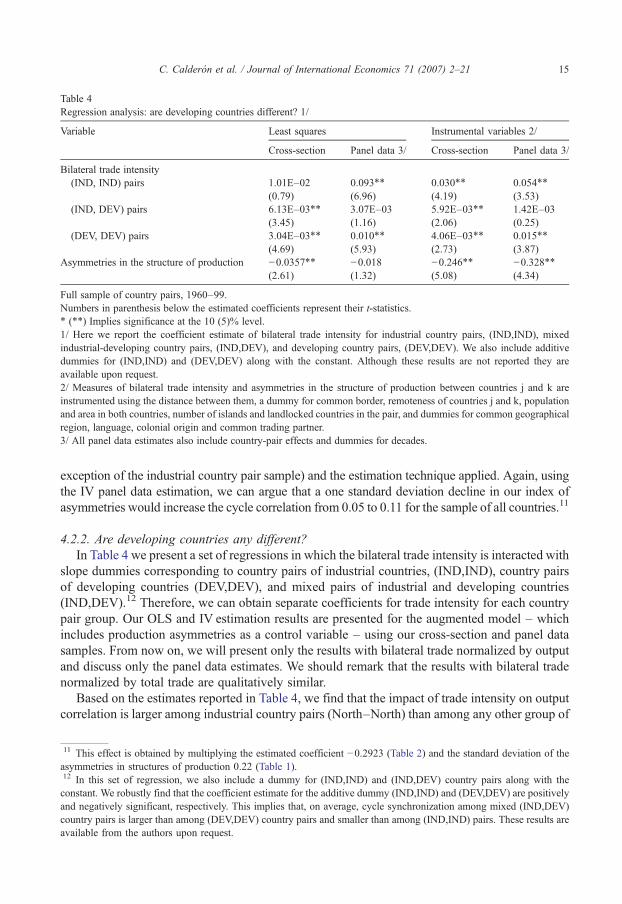
Table 4Regression analysis: are developing countries different? 1/

Variable Least squares Instrumental variables 2/

Cross-section Panel data 3/ Cross-section Panel data 3/

Bilateral trade intensity(IND, IND) pairs 1.01E–02 0.093⁎⁎ 0.030⁎⁎ 0.054⁎⁎

(0.79) (6.96) (4.19) (3.53)(IND, DEV) pairs 6.13E–03⁎⁎ 3.07E–03 5.92E–03⁎⁎ 1.42E–03

(3.45) (1.16) (2.06) (0.25)(DEV, DEV) pairs 3.04E–03⁎⁎ 0.010⁎⁎ 4.06E–03⁎⁎ 0.015⁎⁎

(4.69) (5.93) (2.73) (3.87)Asymmetries in the structure of production −0.0357⁎⁎ −0.018 −0.246⁎⁎ −0.328⁎⁎

(2.61) (1.32) (5.08) (4.34)

Full sample of country pairs, 1960–99.Numbers in parenthesis below the estimated coefficients represent their t-statistics.⁎ (⁎⁎) Implies significance at the 10 (5)% level.1/ Here we report the coefficient estimate of bilateral trade intensity for industrial country pairs, (IND,IND), mixedindustrial-developing country pairs, (IND,DEV), and developing country pairs, (DEV,DEV). We also include additivedummies for (IND,IND) and (DEV,DEV) along with the constant. Although these results are not reported they areavailable upon request.2/ Measures of bilateral trade intensity and asymmetries in the structure of production between countries j and k areinstrumented using the distance between them, a dummy for common border, remoteness of countries j and k, populationand area in both countries, number of islands and landlocked countries in the pair, and dummies for common geographicalregion, language, colonial origin and common trading partner.3/ All panel data estimates also include country-pair effects and dummies for decades.


exception of the industrial country pair sample) and the estimation technique applied. Again, usingthe IV panel data estimation, we can argue that a one standard deviation decline in our index ofasymmetries would increase the cycle correlation from 0.05 to 0.11 for the sample of all countries.11

4.2.2. Are developing countries any different?In Table 4 we present a set of regressions in which the bilateral trade intensity is interacted with

slope dummies corresponding to country pairs of industrial countries, (IND,IND), country pairsof developing countries (DEV,DEV), and mixed pairs of industrial and developing countries(IND,DEV).12 Therefore, we can obtain separate coefficients for trade intensity for each countrypair group. Our OLS and IV estimation results are presented for the augmented model – whichincludes production asymmetries as a control variable – using our cross-section and panel datasamples. From now on, we will present only the results with bilateral trade normalized by outputand discuss only the panel data estimates. We should remark that the results with bilateral tradenormalized by total trade are qualitatively similar.

Based on the estimates reported in Table 4, we find that the impact of trade intensity on outputcorrelation is larger among industrial country pairs (North–North) than among any other group of

11 This effect is obtained by multiplying the estimated coefficient −0.2923 (Table 2) and the standard deviation of theasymmetries in structures of production 0.22 (Table 1).12 In this set of regression, we also include a dummy for (IND,IND) and (IND,DEV) country pairs along with theconstant. We robustly find that the coefficient estimate for the additive dummy (IND,IND) and (DEV,DEV) are positivelyand negatively significant, respectively. This implies that, on average, cycle synchronization among mixed (IND,DEV)country pairs is larger than among (DEV,DEV) country pairs and smaller than among (IND,IND) pairs. These results areavailable from the authors upon request.

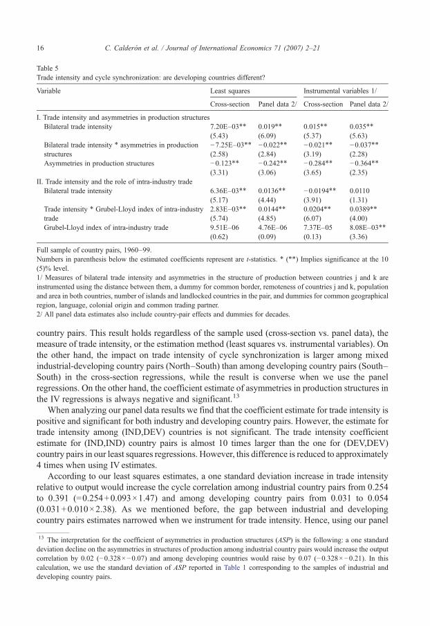
Table 5Trade intensity and cycle synchronization: are developing countries different?

Variable Least squares Instrumental variables 1/

Cross-section Panel data 2/ Cross-section Panel data 2/

I. Trade intensity and asymmetries in production structuresBilateral trade intensity 7.20E–03⁎⁎ 0.019⁎⁎ 0.015⁎⁎ 0.035⁎⁎

(5.43) (6.09) (5.37) (5.63)Bilateral trade intensity ⁎ asymmetries in productionstructures

−7.25E–03⁎⁎ −0.022⁎⁎ −0.021⁎⁎ −0.037⁎⁎(2.58) (2.84) (3.19) (2.28)

Asymmetries in production structures −0.123⁎⁎ −0.242⁎⁎ −0.284⁎⁎ −0.364⁎⁎(3.31) (3.06) (3.65) (2.35)

II. Trade intensity and the role of intra-industry tradeBilateral trade intensity 6.36E–03⁎⁎ 0.0136⁎⁎ −0.0194⁎⁎ 0.0110

(5.17) (4.44) (3.91) (1.31)Trade intensity ⁎ Grubel-Lloyd index of intra-industrytrade

2.83E–03⁎⁎ 0.0144⁎⁎ 0.0204⁎⁎ 0.0389⁎⁎

(5.74) (4.85) (6.07) (4.00)Grubel-Lloyd index of intra-industry trade 9.51E–06 4.76E–06 7.37E–05 8.08E–03⁎⁎

(0.62) (0.09) (0.13) (3.36)

Full sample of country pairs, 1960–99.Numbers in parenthesis below the estimated coefficients represent are t-statistics. ⁎ (⁎⁎) Implies significance at the 10(5)% level.1/ Measures of bilateral trade intensity and asymmetries in the structure of production between countries j and k areinstrumented using the distance between them, a dummy for common border, remoteness of countries j and k, populationand area in both countries, number of islands and landlocked countries in the pair, and dummies for common geographicalregion, language, colonial origin and common trading partner.2/ All panel data estimates also include country-pair effects and dummies for decades.


country pairs. This result holds regardless of the sample used (cross-section vs. panel data), themeasure of trade intensity, or the estimation method (least squares vs. instrumental variables). Onthe other hand, the impact on trade intensity of cycle synchronization is larger among mixedindustrial-developing country pairs (North–South) than among developing country pairs (South–South) in the cross-section regressions, while the result is converse when we use the panelregressions. On the other hand, the coefficient estimate of asymmetries in production structures inthe IV regressions is always negative and significant.13

When analyzing our panel data results we find that the coefficient estimate for trade intensity ispositive and significant for both industry and developing country pairs. However, the estimate fortrade intensity among (IND,DEV) countries is not significant. The trade intensity coefficientestimate for (IND,IND) country pairs is almost 10 times larger than the one for (DEV,DEV)country pairs in our least squares regressions. However, this difference is reduced to approximately4 times when using IV estimates.

According to our least squares estimates, a one standard deviation increase in trade intensityrelative to output would increase the cycle correlation among industrial country pairs from 0.254to 0.391 (=0.254+0.093×1.47) and among developing country pairs from 0.031 to 0.054(0.031+0.010×2.38). As we mentioned before, the gap between industrial and developingcountry pairs estimates narrowed when we instrument for trade intensity. Hence, using our panel

13 The interpretation for the coefficient of asymmetries in production structures (ASP) is the following: a one standarddeviation decline on the asymmetries in structures of production among industrial country pairs would increase the outputcorrelation by 0.02 (−0.328×−0.07) and among developing countries would raise by 0.07 (−0.328×−0.21). In thiscalculation, we use the standard deviation of ASP reported in Table 1 corresponding to the samples of industrial anddeveloping country pairs.


IV estimates and normalizing bilateral trade by total output we find that one standard deviationincrease in the measure of bilateral trade intensity from the initial mean will generate an increasein output correlation: (a) from 0.254 to 0.332 (=0.254+0.054×1.46) among industrial country pairs,(b) from 0.075 to 0.077 (=0.075+0.001×1.23) among mixed industrial-developing country pairs,and (c) from 0.031 to 0.052 (=0.031+0.015×1.39) for developing country pairs.14

From these results there are two important implications relative to previous studies. First, ourfinding for industrial countries is very similar to the results in Frankel and Rose (1998). Second,our regression results confirm our priors: The impact of trade integration among developingcountries is still positive and significant. Finally, we reject the null of equal coefficients for tradeintensity of industrial- and developing-country pairs. In fact, the coefficient for developingcountry pairs is significantly smaller.15

4.2.3. Production structure asymmetries, intra-industry trade, and the link between tradeintensity and cycle correlation

In the previous section, we presented evidence suggesting that the link between trade intensityand cycle correlation is stronger in the case of industrial countries. In the conceptual discussion in theIntroduction, we discussed some ideas regarding the reasons why the link would be weaker incountry pairs involving developing countries. Specifically, we expected the effect to depend on thepattern of trade and specialization in the country pair. Developing and mixed country pairs wereexpected to have more asymmetric production structures, and a lower degree of intra-industry trade(these expectations were confirmed by the descriptive statistics presented in Table 1). In thesecountry pairs, increased trade intensity was expected to lead to increased specialization in differentindustries, which in turn would lead to asymmetric effects of industry-specific shocks. In contrast, inthe case of industrial countries, increased trade intensity may lead to intra-industry specialization, inwhich case industry-specific shocks may affect both countries in the pair in the same way. In thissection, we will explore the role of production asymmetries, and intra-industry trade, in an explicitway. In addition, wewill discuss the extent towhich the differences found between industrial countrypairs and developing country pairs can be attributed to these factors.

4.2.3.1. Production structure asymmetries. In our previous regression analysis, we haveincluded the index of production asymmetries as a control variable. However, as argued above,similarities in the production structure may affect the nature of the impact of trade integration oncycle correlation, since similar economies are more prone to show a pattern of intra-industryspecialization. These considerations suggest the convenience of adding an interactive term, inorder to look at complementarities between production asymmetries and trade intensity. Thus, Eq.(4) is modified as follows:

qðyCi ;yCj Þ ¼ ai;j þ bs þ gT ki;j;τ þ wTi;j;s

kdASPi;j;sþ /ASPi;j;sþ ui;j;s ð5Þ

We expect the coefficient for the interaction term ψ to be negative and significant, suggestingthat the impact of trade integration should be weaker among countries with dissimilar productionstructures.

14 See the standard deviation of the instrumented bilateral trade normalized by output in Table 1 and the IV panelestimates in the last column of Table 4.15 Test results are available from the authors upon request.


The results of the regressions, in which we also include production asymmetries as a controlvariable, are reported in panel I of Table 5. Consistent with our prior, we find evidence of anegative and statistically significant interaction effect between trade intensity and asymmetries ineconomic structures. This result is robust to the bilateral trade measure used and estimationtechnique applied. Hence, the higher the extent of the asymmetries in economic structures, thelower the change in output correlation that follows a positive surge in trade. In addition, the indexof asymmetries enters separately with a negative and significant coefficient in all the regressions.

The panel IV regression estimates suggest that if the index of production asymmetries is equalto 0 (countries in the pair with identical production structures), the estimated impact will be givenby the coefficient of bilateral trade intensity, which is equal to 0.035. At the mean of productionasymmetries for the whole sample of country pairs (corresponding to an index of 0.399, accordingto Table 1), the estimated impact would be 0.021 (=0.035–0.037⁎0.399). Our results also suggestthat the impact of trade intensity on cycle correlation could even become negative for a pair ofcountries that are sufficiently dissimilar. Specifically, the impact would turn negative for countrypairs for which the index of production asymmetries is greater than 0.96. It is worth noting,however, that while the index of production asymmetries could potentially vary between 0 and 2,only 7% of the country pairs have an index above the 0.96 threshold (and none of thesecorrespond to industrial country pairs).

To what extent do differences in production asymmetries account for the differences acrosscountry groups in the impact of trade intensity on cycle correlation reported in Table 4? To answerthis question, recall from Table 1 that the mean of production asymmetries corresponding toindustrial country pairs is 0.133, while the mean corresponding to developing country pairs is0.393. This suggests that the estimated coefficient for the impact of trade intensity on cyclecorrelation would be 0.03 (=0.035–0.037⁎0.133) for industrial country pairs, and 0.021(=0.035–0.037⁎0.393) for developing country pairs. We should note that the estimate forindustrial country pairs is smaller than the one reported in Table 8 (0.035 vs. 0.054), while it isslightly larger for developing country pairs (0.021 vs. 0.015).

These simple calculations suggest that differences in production structure asymmetries seem toaccount for almost 40% of the differences between industrial country pairs and developingcountry pairs regarding the estimated impact of a given change in trade intensity on cyclecorrelation.

4.2.3.2. Intra-industry trade. The results of the previous section suggest that the differencebetween industrial and developing country pairs regarding the link between trade intensity andcycle correlation can be traced to differences in the pattern of specialization across country pairs.The 9-sector index of production asymmetries used above, however, is a very rough measure ofspecialization. In this section, we conduct a similar exercise, using the Grubel and Lloyd index ofintra-industry trade in place of the index of production asymmetries. An advantage of the index ofintra-industry trade is that it is built on the basis of much more disaggregated (4-digit SITC) tradedata.16 An important disadvantage, however, is that the index of intra-industry trade is availableonly for the last two decades of our sample. This translates into only two data points per countrypair, which limits the precision with which we estimate our panel data coefficients that, as arguedabove, are the ones that provide answers to the “right policy question”.

16 The panel correlation between the Grubel-Lloyd index of intra-industry trade and the 9-sector index of productionasymmetries is −0.20.


In order to check the role of intra-industry trade in the link between trade intensity and cyclecorrelation, we run a modified version of the model in Eq. (5), replacing the index of productionasymmetries by the index of intra-industry trade. This analysis extends and complements em-pirical evidence for industrial economies (Fidrmuc, 2002; Gruben et al., 2002) and for East Asia(Shin and Wang, 2002, 2003). These authors find that output correlation is higher in country pairswith a higher degree of intra-industry trade.

Here, we run the following regression equation:

qðyCi ;yCj Þ ¼ ai;j þ bs þ gT ki;j;s þ wTk

i;j;sd GLIi;j;s þ /GLIi;j;s þ ui;j;s ð6Þ

In contrast to the case of the production asymmetries, here we expect ψ in this framework (theparameter associated to the interaction between trade intensity and intra-industry trade) to bepositive and significant. As in the case of the analysis of production asymmetries, the modelincludes a separate intra-industry trade term, to control for the direct effect of this variable oncycle correlation. The results are presented in panel II of Table 5.

The coefficient for the interactive term, ψ, is always positive and significant; however, themagnitude of the effect varies substantially depending on the model. On the other hand, thecoefficient of bilateral trade in the IV regression – which represents the impact of inter-industrytrade for GLI equal to zero – is negative but statistically not different from zero.

Focusing on the last regression in this table (IV, panel data, using total output to normalizebilateral trade), the impact of trade intensity on cycle correlation could potentially vary between0.011 (for countries with no intra industry trade) and 0.05 (for country pairs with an GLI indexof 1).17

To what extent are differences across groups of countries explained by differences in intra-industry trade? According to Table 1, the index of intra-industry trade averages 0.208 for industrialcountry pairs, and 0.009 for developing country pairs. In the case in which total output is used tocalculate trade intensities, this translates into an estimated impact of 0.019 for industrial countrypairs, and 0.011 for developing country pairs. These coefficients are not strictly comparable to thoseof Table 4 (which are estimated for the full four-decade sample period); however, we reestimate thecorresponding equation of Table 4 for the period 1980–99 and found that the coefficient estimate forinternational trade integration was 0.015 for developing country pairs and 0.042 for industrialcountry pairs.18 These results suggest that approximately 30% of the differences between countrypair groups can be accounted for by differences in the index of intra-industry trade.

5. Conclusions

While several authors find that trade intensity increases cycle correlation among industrialcountries, there are reasons to believe that this could be different among developing countries andamong industrial-developing country pairs. Different patterns of specialization and bilateral trade

17 Note that 0.05 is the sum of the coefficient of trade intensity and that corresponding to the interactive term. Also, incontrast to the case of production asymmetries, in which the results were nearly identical, here it makes a difference if wenormalize using total trade. The impact would range between −0.003, for country pairs with no intra-industry trade to0.051, for country pairs with an index of 1.18 When reestimating the regressions in Table 4 for the period 1980–99 the results are qualitatively similar. Theregressions are not reported but are available from the authors upon request.


among country pairs involving developing countries suggest that, in these cases, the impact oftrade intensity on cycle correlation should be weaker, and of ambiguous sign.

In this paper we have attempted to provide an exhaustive analysis of the impact of tradeintegration on business cycle synchronization. We provide an efficient estimate for this effect(thanks to the use of the gravity equation for international trade). We assess the nature of therelationship between trade integration and output correlation for different samples of countrypairs and we include interaction effects between trade intensity and direct sectoral linkages.

First, looking at the whole sample, we find that countries that have closer trade linkages exhibithigher output co-movement. This result is robust to changes in our measures of bilateral trade andcyclical output, as well as the estimation method chosen. An economic interpretation of this resultyields an increase in business cycle correlations from 0.05 to 0.085 if the bilateral trade intensityincreases in one standard deviation.

Second, the impact of trade integration on cyclical output correlation among industrialcountries is higher than the impact among developing countries and the impact for industrial-developing country pairs. A one standard deviation increase in bilateral trade intensity (nor-malized by total output in countries i and j) raises cyclical output correlation from 0.25 to 0.33industrial countries, a result that is of the same order of magnitude as that found by Frankel andRose (1998). On the other hand, the same increase in bilateral trade (when normalized by output)would lead to a negligible increase in output correlation from 0.075 to 0.077 for the industrial-developing country pairs, while it increased from 0.031 to 0.052 for developing country pairs.

Third, we find robust evidence of interaction effects between trade intensity and asymmetries inthe economic structures across countries. After we account for these asymmetries, we find that a onestandard deviation increase in bilateral trade (normalized by output) would raise output correlationsfrom0.05 to 0.08 for the full sample of country pairs. Also, a similar shockwould increase the outputcorrelation from 0.25 to 0.3 among industrial countries, and from 0.03 to 0.06 among developingcountries. Fourth, we find that the response of output correlation to trade integration is higher incountry pairs with a higher degree of intra-industry trade. This result is robust to the measure,specification or estimation technique used, and it is consistent with the findings of Gruben et al.(2002) and Fidrmuc (2002). Our estimates suggest that, after accounting for the degree of intra-industry trade, a one standard deviation increase in bilateral trade (normalized by output) would raiseoutput correlations from 0.05 to 0.07. A similar shock would increase the output correlation from0.25 to 0.282 among industrial countries, and from 0.03 to 0.047 among developing countries.

Finally, we find that a significant part of the difference in the impact of trade intensity onbusiness cycle synchronization between industrial and developing-country pairs is explained bydifferences in the structures of production and the degree of intra-industry trade. When weevaluate their interaction with trade intensity separately, our results suggest that approximately40% of these differences can be attributed to asymmetries in structures of production, whereas30% can attributed to the extent of intra-industry trade.

References

Baxter, M., King, R.G., 1999. Measuring business cycles: approximate band-pass filters for economic time series. TheReview of Economics and Statistics 81, 575–593.

Clark, T.E., van Wincoop, E., 2001. Borders and business cycles. Journal of International Economics 55, 59–85.Coe, D.T., Helpman, E., 1995. International R&D spillovers. European Economic Review 39, 859–887.Deardorff, A.V., 1998. Determinants of bilateral trade: does gravity work in a neoclassical world? In: Frankel, J.A. (Ed.),

The Regionalization of the World Economy. University of Chicago Press, Chicago, IL, pp. 7–22.


Eichengreen, B., Irwin, D.A., 1998. The role of history in bilateral trade flows. In: Frankel, J.A. (Ed.), The Regionalizationof the World Economy. University of Chicago Press, Chicago, IL, pp. 33–57.

Fatás, A., 1997. EMU: countries or regions? Lessons from the EMS experience. European Economic Review 41, 743–751.Fidrmuc, J., 2002. The Endogeneity of optimum currency area criteria, intra-industry trade and EMU enlargement. Oester-

reiche Nationalbank, Mimeo. February.Frankel, J., Romer, D., 1999. “Does trade cause growth?”. American Economic Review 89 (3), 379–399.Frankel, J.A., Rose, A.K., 1997. Is EMU justifiable ex post than ex ante? European Economic Review 41, 753–760.Frankel, J.A., Rose,A.K., 1998. The endogeneity of the optimumcurrency area criteria. The Economic Journal 108, 1009–1025.Frankel, J.A., Rose, A.K., 2002. An estimate of the effect of common currencies on trade and income. Quarterly Journal of

Economics 117, 437–466.Glick, R., Rose, A.K., 2002. Does a currency union affect trade? The time-series evidence. European Economics Review

46, 1125–1151.Grubel, H.G., Lloyd, P.J., 1975. Intra-Industry Trade: The Theory and Measurement of International Trade in Differ-

entiated Products. John Wiley & Sons, London.Gruben, W.C., Koo, J., Millis, E., 2002. How much does international trade affect business cycle synchronization? Federal

Reserve Bank of Dallas Research Department Working Paper, vol. 0203. August.Imbs, J., 2001. Co-fluctuations. CEPR Discussion Paper, vol. 2267. October.Imbs, J., 2004. Trade, finance, specialization, and synchronization. The Review of Economics and Statistics 86, 723–734.Kalemli-Ozcan, S., Sorensen, B.E., Yosha, O., 2001. Economic integration, industrial specialization, and the asymmetry of

macroeconomic fluctuations. Journal of International Economics 55, 107–137.Kose, M.A., Yi, K.-M., 2001. International trade and business cycles: is vertical specialization the missing link. American

Economic Review Papers and Proceedings 371–375.Krugman, P., 1991. Geography and Trade. The MIT Press, Cambridge, MA.Krugman, P., 1993. Lesson of Massachusetts for EMU. In: Giavazzi, F., Torres, F. (Eds.), The Transition to Economic and

Monetary Union in Europe. Cambridge University Press, New York, pp. 241–261.Lichtenberg, F., van Pottelsberghe, B., 1998. International R&D spillovers: a comment. European Economic Review 42,

1483–1491.Rose, A.K., Engel, C., 2002. Currency unions and international integration. Journal of Money, Credit and Banking 34 (3),

804–826 . August.Shin, K., Wang, Y., 2002. Trade integration and business cycle comovements: the case of Korea with other Asian

countries. KIEP Working Paper, vol. 02-08. Korea Institute for International Economic Policy.Shin, K., Wang, Y., 2003. Trade integration and business cycle synchronization in East Asia. Discussion Paper, vol. 574.

The Institute of Social and Economic Research, Osaka University. March.Stein, E., Weinhold, D., 1998. Canadian–U.S. Border effects and the gravity equation model of trade. Washington, DC:

Inter-American Development Bank. Mimeo. February.Stockman, A.C., 1988. Sectoral and national aggregate disturbances to industrial output in seven European countries.

Journal of Monetary Economics 21, 387–410.Wei, S.-J., 1996. Intra-national versus international trade: how stubborn are nations in global integration? NBERWorking

Paper, vol. 5531. April.

Documents

Trade intensity and business cycle synchronization: Are developing countries any different?