Embed Size (px)
Citation preview

Faculdade de Engenharia da Universidade do Porto
Traction Control in Electric Vehicles
Tiago Oliveira Bastos Pinto de Sá
Dissertation prepared under the
Master in Electrical and Computers Engineering
Major Automation
Supervisor: Adriano Carvalho
July 2012

ii
© Tiago Sá, 2012


iii
To my mother and grandma

iv

v
Resumo
O sector dos transportes é um dos maiores setores industriais hoje em dia. Desde o
desenvolvimento do motor de combustão interna e da sua aplicação ao setor dos transportes,
as pessoas estão cada vez mais dependentes de uma forma económica e confortável de viajar.
Com o aumento do preço dos combustíveis fósseis causado pela sua procura excessiva, e
com as recentes preocupações ambientais relativas à emissão de gases poluentes gerados pela
queima do combustível, a existência de uma alternativa é fulcral. A forma de transporte
alternativo mais comum num ambiente urbano é o autocarro. É mais barato, mais
conveniente em determinados casos e produz menos poluição per capita do que um carro
próprio. No entanto, continua a poluir.
Com isto em mente, e com a recente eminência dos motores elétricos no setor dos
transportes, é analisado o controlo de motores síncronos de ímanes permanentes, em
particular a aplicação de um de 150kW num autocarro elétrico. O objetivo deste documento é
analisar o domínio do controlo na mobilidade elétrica e discutir o projeto do controlador que
alimenta o motor, permitindo o seu acionamento e travagem, com a possibilidade de
regenerar a energia da travagem, recarregando dessa forma as baterias. O sistema deverá ser
capaz de funcionar sem sensores de velocidade ou posição.
Pretende-se validar os resultados obtidos na simulação aplicando um motor menos
potente do que o objetivo final, de forma a poder validar laboratorialmente esses mesmos
resultados. O propósito final deste trabalho é ser implementado num autocarro elétrico da
empresa CaetanoBus, melhorando desta forma o sistema de tração já existente.

vi

vii
Abstract
Transportation sector is one of the biggest industrial sectors nowadays. Since the
development of the internal combustion engine and its application in the transportation
sector, people are becoming more dependent on a more economic and comfortable way of
traveling.
With the constant increase in fossil fuels’ price caused by the excessive demand, and with
recent environmental concerns relatively to toxic gases emissions, the search of alternative
ways of locomotion becomes crucial. Urban buses are the most common alternative to the
usage of own vehicle. However, they still produce toxic gases.
Having this in consideration and taking advantage of the recent eminence of electric
motors on transportation sector, it is analyzed the control of permanent magnet synchronous
motors, in particular an application of a 150kW motor on an electric bus. This document aims
at analyzing the control domain in electric mobility and discussing the design of the controller
that drives the motor, allowing its driving and braking, with the ability to regenerate braking
energy for recharging the batteries. The system should be capable of working without speed
or position sensors.
It is intended to validate the simulation results applying a less powerful motor than the
one to be used as the final objective, in order to achieve a laboratorial validation of those
results. The final purpose of this work is to be applied in an electric bus from the company
CaetanoBus, enhancing the traction control already existent.

viii

ix
Acknowledgments
I would like to express my gratitude to my supervisor Adriano da Silva Carvalho for his
guidance and suggestions along the development of this work.
I wish to thank my teammate and friend Ricardo Soares who also collaborate in the
development of the work, for his constant high motivation level and exchange of ideas.
I want to give my most special thanks to my lovely girlfriend Cátia Albergaria for being
there every time I needed and for her constant encouragement.
To all my friends and comrades for all the great moments provided all over the years, for
the help and motivation given in the worst times, for the knowledge sharing and essentially
for being part of my life. It has been a pleasure.
Finally, to my family I would like to sincerely thank, specially my brother who always
supported me, and my mother and grandmother who have always been there in every stage of
my life and made possible the journey of the last 5 years in this University. To them I
dedicate this thesis.

x

xi
Contents
RESUMO ......................................................................................................................................... V
ABSTRACT ..................................................................................................................................... VII
ACKNOWLEDGMENTS .................................................................................................................... IX
CONTENTS...................................................................................................................................... XI
LIST OF FIGURES ........................................................................................................................... XIII
LIST OF TABLES .............................................................................................................................. XV
ABBREVIATIONS AND SYMBOLS .................................................................................................. XVII
CHAPTER 1 ...................................................................................................................................... 1
INTRODUCTION ...................................................................................................................................... 1
1.1. Motivation ........................................................................................................................ 1
1.2. About the Project ............................................................................................................. 2
1.3. Document Structure ......................................................................................................... 2
CHAPTER 2 ...................................................................................................................................... 5
ELECTRICAL TRACTION IN THE POWER TRAIN ............................................................................................... 5
2.1. System Overview .............................................................................................................. 5
2.2. System Requirements ....................................................................................................... 8
2.3. Electronic Power Converters (EPC) ................................................................................... 9 2.3.1. “High Efficiency” Converters ........................................................................................................... 9 2.3.2. DC/DC ZVS Bidirectional Converter with Phase-Shift + PWM ....................................................... 11 2.3.3. Improved DC/DC buck/boost Bidirectional Converter ................................................................... 12 2.3.4. Isolated Full Bridge Converter ....................................................................................................... 12 2.3.5. Three-phase Inverter ..................................................................................................................... 13
2.4. Types of Control ............................................................................................................. 13
2.5. Market Research ............................................................................................................ 17 2.5.1. Selling of the Regenerative Braking System .................................................................................. 17 2.5.2. Electric Vehicles With Regenerative Braking ................................................................................. 17
2.6. Summary ........................................................................................................................ 18
CHAPTER 3 .................................................................................................................................... 19
PERMANENT MAGNET SYNCHRONOUS MOTOR ......................................................................................... 19
3.1. Introduction .......................................................................................................................... 19
3.2. Types of Permanent Magnet Synchronous Motors .............................................................. 20
3.3. PMSM Modeling ................................................................................................................... 22
3.4. Definitions of Torque Angle .................................................................................................. 26

xii
3.5. Relations Between Torque Angle, Current and Air-gap Flux ................................................ 28 3.5.1. Torque dependability on and ................................................................................................ 28 3.5.2. Torque dependability on .......................................................................................................... 29
3.6. Used Motor’s Parameters and Simulation ........................................................................... 29
3.7. Summary .............................................................................................................................. 30
CHAPTER 4 .................................................................................................................................... 31
CONTROL OF THE PMSM ...................................................................................................................... 31
4.1. Introduction .......................................................................................................................... 31
4.2. Control Strategy ................................................................................................................... 32 4.2.1. Control Methods ........................................................................................................................... 32 4.2.2. Control Signal Generation for the Inverter .................................................................................... 36 4.2.3. Controllers’ Tuning ........................................................................................................................ 41
4.3. Controller platform ............................................................................................................... 45
4.4. Partial Results Analysis ......................................................................................................... 47 4.4.1. Stator current vector angle ( ) at 90 degrees with sine-PWM..................................................... 48 4.4.2. Air-gap flux vector angle ( ) at 90 degrees with sine-PWM ........................................................ 49 4.4.3. MTPA with sine-PWM ................................................................................................................... 50 4.4.4. MTPA with SVM............................................................................................................................. 52
4.5. System Behavior Based on Power Balance ........................................................................... 53 4.5.1. Power definitions .......................................................................................................................... 53 4.5.2. Mathematical Expressions ............................................................................................................ 54 4.5.3. P-Q Theory .................................................................................................................................... 56 4.5.4. Power Control ............................................................................................................................... 57
4.6. Summary .............................................................................................................................. 60
CHAPTER 5 .................................................................................................................................... 63
SYSTEM SENSORLESS CONTROL ............................................................................................................... 63
5.1. Introduction .......................................................................................................................... 63
5.2. Sensorless Techniques Comparison ...................................................................................... 63 5.2.1. Back-EMF Estimator ...................................................................................................................... 64 5.2.2. State Observer ............................................................................................................................... 64 5.2.3. Sliding-mode Observer .................................................................................................................. 65 5.2.4. High-frequency Signal Injection..................................................................................................... 65 5.2.5. PLL-based Estimator ...................................................................................................................... 66
5.3. Sensorless Control Results .................................................................................................... 68
5.4. Summary .............................................................................................................................. 71
CHAPTER 6 .................................................................................................................................... 73
SYSTEM VALIDATION ............................................................................................................................. 73
6.1. Introduction .......................................................................................................................... 73
6.2. Regenerative Braking ........................................................................................................... 73
6.3. System Performance Detailed Analysis ................................................................................ 77
6.4. Hardware Implementation ................................................................................................... 81
6.5. Summary .............................................................................................................................. 83
CHAPTER 7 .................................................................................................................................... 85
CONCLUSION ....................................................................................................................................... 85
7.1. Final Conclusions .................................................................................................................. 85
7.2. Future Work ......................................................................................................................... 87
REFERENCES .................................................................................................................................. 89

xiii
List of Figures
FIG 2.1 – SCHEMATIC OF A GENERIC ELECTRIC VEHICLE’S COMPONENTS WITH POSSIBLE SOLUTIONS [1]. ............................ 5
FIG 2.2 – RELATIONAL SCHEMATIC OF GENERIC ELECTRIC VEHICLE COMPONENTS [1]. ..................................................... 6
FIG 2.3 – BLDC AND PMSM STATOR FLUX LINKAGE AND BACK-EMF WAVEFORMS [2]. ................................................ 7
FIG 2.4 – SEVERAL HIGH EFFICIENCY SWITCHING CONVERTERS’ TOPOLOGIES [3]. ......................................................... 10
FIG 2.5 – IMPROVED HIGH EFFICIENCY CONVERTERS TOPOLOGIES: UNIDIRECTIONAL (FROM A TO C) AND BIDIRECTIONAL (D)
[3]. ...................................................................................................................................................... 11
FIG 2.6 - DC/DC ZVS BIDIRECIONAL CONVERTER [4]. .......................................................................................... 11
FIG 2.7 – IMPROVED DC/DC BUCK/BOOST BIDIRECTIONAL CONVERTER [5]. .............................................................. 12
FIG 2.8 – ISOLATED FULL BRIDGE CONVERTER. ...................................................................................................... 12
FIG 2.9 - THREE-PHASE INVERTER TO BE USED, WITH BRAKING CHOPPER AND DC LINK FILTER. ....................................... 13
FIG 2.10 - REPRESENTATION OF , AND , AS THEIR DQ COMPONENTS AND ANGLES RELATIONS AT A RANDOM POINT OF
OPERATION. MODULES MUST NOT BE CONSIDERED. ....................................................................................... 15
FIG 3.1 – ROTOR ARRANGEMENTS OF PMSM: A) SURFACE MOUNTED (SPM), B) INSET SURFACE MOUNTED AND C) INTERIOR
MOUNTED (IPM) [6]............................................................................................................................... 20
FIG 3.2 – IPM ROTOR WITH FOUR POLES WITH A) TANGENTIALLY MAGNETIZED PMS AND B) RADIALLY MAGNETIZED PMS [6].
........................................................................................................................................................... 21
FIG 3.3 – MAGNETIC FLUX PATHS IN A) SPM MOTOR AND B) IPM MOTOR [7]. ......................................................... 22
FIG 3.4 – REPRESENTATION OF THE THREE REFERENCE FRAMES: THREE-PHASE, DQ AND ΑΒ. D-AXIS ALIGNED WITH ROTOR
FLUX. Α-AXIS ALIGNED WITH PHASE-A. ......................................................................................................... 24
FIG 3.5 – D AND Q REPRESENTATION CIRCUITS OF A PMSM.................................................................................... 25
FIG 3.6 – DLL MODEL OF PMSM IN PSIM SOFTWARE. ......................................................................................... 30
FIG 4.1 - PSIM CONTROL SCHEME WITH VECTOR AT 90 DEGREES METHOD. ........................................................... 34
FIG 4.2 - PSIM CONTROL SCHEME WITH AT 90 DEGREES METHOD....................................................................... 35
FIG 4.3 - PSIM CONTROL SCHEME WITH MTPA METHOD. ..................................................................................... 36
FIG 4.4 - SVM STATES ACCORDING TO INVERTER’S TRANSISTORS STATE. .................................................................... 38
FIG 4.5 - SVM SEQUENCE FOR ODD SECTOR. ....................................................................................................... 40
FIG 4.6 - SVM SEQUENCE FOR EVEN SECTOR. ...................................................................................................... 40
FIG 4.7 – SVM MODEL DESIGNED IN PSIM WITH DIFFERENT STEPS HIGHLIGHTED. ...................................................... 40
FIG 4.8 – SIMPLIFIED BLOCK DIAGRAM OF THE SYSTEM. .......................................................................................... 43
FIG 4.9 – SIMPLIFIED SYSTEM IMPLEMENTED IN SIMULINK. ..................................................................................... 43
FIG 4.10 – REPRESENTATION OF FPGA ARCHITECTURE. ......................................................................................... 46
FIG 4.11 – TORQUE REFERENCE AND LOAD TORQUE PATTERN. EXPECTED SPEED BEHAVIOR. .......................................... 47
FIG 4.12 - RESULTS FOR AT 90º WITH SINE-PWM. TOP GRAPHIC: TORQUE PRODUCED, LOAD TORQUE AND ROTOR
ANGULAR SPEED; BOTTOM GRAPHIC: AND . ........................................................................................... 48
FIG 4.13 - RESULTS FOR AT 90º WITH SINE-PWM. TOP GRAPHIC: STATOR CURRENT ANGLE AND AIR-GAP FLUX ANGLE
; BOTTOM GRAPHIC: AND MODULES. ................................................................................ 49
FIG 4.14 - RESULTS FOR AT 90º WITH SINE-PWM. TOP GRAPHIC: TORQUE PRODUCED, LOAD TORQUE AND ROTOR
ANGULAR SPEED; BOTTOM GRAPHIC: AND . ........................................................................................... 49
FIG 4.15 - RESULTS FOR AT 90º WITH SINE-PWM. TOP GRAPHIC: STATOR CURRENT ANGLE AND AIR-GAP FLUX ANGLE
; BOTTOM GRAPHIC: AND MODULES. ................................................................................ 50
FIG 4.16 - RESULTS FOR WITH SINE-PWM. TOP GRAPHIC: TORQUE PRODUCED, LOAD TORQUE AND ROTOR ANGULAR
SPEED; BOTTOM GRAPHIC: AND . ........................................................................................................ 51

xiv
FIG 4.17 - RESULTS FOR WITH SINE-PWM. TOP GRAPHIC: STATOR CURRENT ANGLE AND AIR-GAP FLUX ANGLE ;
BOTTOM GRAPHIC: AND MODULES. ...................................................................................... 51
FIG 4.18 - RESULTS FOR MTPA WITH SVM. TOP GRAPHIC: TORQUE PRODUCED, LOAD TORQUE AND ROTOR ANGULAR SPEED;
BOTTOM GRAPHIC: AND . .................................................................................................................. 52
FIG 4.19 - RESULTS FOR MTPA WITH SVM. TOP GRAPHIC: STATOR CURRENT ANGLE AND AIR-GAP FLUX ANGLE ;
BOTTOM GRAPHIC: AND MODULES. ...................................................................................... 52
FIG 4.20 – POWER TRIANGLE ........................................................................................................................... 55
FIG 4.21 – SENSORLESS CONTROL BASED ON POWER BALANCE. TOP LEFT: ELECTROMAGNETIC TORQUE CALCULUS; TOP RIGHT:
DYNAMIC FILTER GAIN; BOTTOM LEFT: ACTIVE POWER CALCULUS; BOTTOM RIGHT: REACTIVE POWER CALCULUS. ...... 58
FIG 4.22 - BODE DIAGRAM OF A FIRST-ORDER LOW-PASS FILTER. = 5HZ. .............................................................. 59
FIG 4.23 – BODE DIAGRAM OF A SECOND-ORDER LOW-PASS FILTER. = 5HZ. .......................................................... 60
FIG 5.1 – PLL-BASED ESTIMATOR LOGIC [8]. ....................................................................................................... 66
FIG 5.2 - PLL-BASED SENSORLESS SPEED AND POSITION ESTIMATOR IMPLEMENTED IN SIMULINK. ................................... 69
FIG 5.3 - SENSORLESS OPERATION. TOP GRAPHIC: TORQUE PRODUCED AND LOAD TORQUE. BOTTOM GRAPHIC: AND . 70
FIG 5.4 – SENSORLESS OPERATION. TOP GRAPHIC: ROTOR ELECTRICAL ANGULAR SPEED (WR – ESTIMATED; WR_REAL –
MEASURED); BOTTOM GRAPHIC: ROTOR ELECTRICAL POSITION (THETA – ESTIMATED; THETA_REAL – MEASURED). ..... 71
FIG 6.1 – PLL-BASED SPEED AND POSITION ESTIMATOR IMPLEMENTED IN PSIM. ........................................................ 74
FIG 6.2 - SENSORLESS OPERATION WITH REGENERATIVE BRAKING. TOP GRAPHIC: TORQUE CALCULATED AND TORQUE
PRODUCED. BOTTOM GRAPHIC: AND . .................................................................................................. 75
FIG 6.3 - SENSORLESS OPERATION. TOP GRAPHIC: ROTOR ELECTRICAL ANGULAR SPEED (WR – ESTIMATED; WR_REAL –
MEASURED); BOTTOM GRAPHIC: ROTOR ELECTRICAL POSITION (THETA – ESTIMATED; THETA_REAL – MEASURED). ..... 75
FIG 6.4 – DETAIL OF THE ESTIMATED POSITION ERROR. .......................................................................................... 76
FIG 6.5 - DC-BUS AVERAGE CURRENT IN TRACTION AND BRAKING, WITH SENSORLESS OPERATION. ............................ 76
FIG 6.6 – RIPPLE DETAIL OF (TOP) TORQUE AND (BOTTOM) STATOR CURRENT, WITH SINE-PWM AT 10KHZ. ................... 77
FIG 6.7 - RIPPLE DETAIL OF (TOP) TORQUE AND (BOTTOM) STATOR CURRENT, WITH SVM AT 10KHZ. ............................. 78
FIG 6.8 – STATOR CURRENT VECTOR ANGLE AND AIR-GAP FLUX VECTOR ANGLE . ................................................. 79
FIG 6.9 – TORQUE ANGLE DETAIL FOR POSITIVE TORQUE. ....................................................................................... 79
FIG 6.10 – TORQUE ANGLE DETAIL FOR NEGATIVE TORQUE. .................................................................................... 80
FIG 6.11 – BACK-EMF PRODUCED BY THE MOTOR. ............................................................................................... 80
FIG 6.12 – REGENERATIVE FEATURE LIKE CRUISE-CONTROL. TOP: TORQUE PRODUCED AND LOAD TORQUE; MIDDLE: ROTOR
ANGULAR SPEED; BOTTOM: DC-BUS CURRENT. ............................................................................................. 81
FIG 6.13 – BLOCK DIAGRAM OF INFINEON HYBRID KIT FOR HYBRIDPACK™1 [9]. ...................................................... 82
FIG 6.14 – INFINEON IGBT DRIVER MODULE FOR HYBRIDPACK™1. ........................................................................ 83

xv
List of Tables
TABLE 1.1 – DISSERTATION STRUCTURE ................................................................................................................ 3
TABLE 2.1 - SUBJECTIVE COMPARISON BETWEEN DIFFERENT TYPES OF MOTORS FOR ELECTRIC VEHICLES APPLICATION (0 TO 5
SCALE) [1]. .............................................................................................................................................. 6
TABLE 3.1 – NOMINAL VALUES OF THE PMSM USED IN SIMULATION. ...................................................................... 29
TABLE 3.2 – PARAMETERS OF THE PMSM USED IN SIMULATION. ............................................................................ 29
TABLE 4.1 – SWITCHING VECTORS COMBINATIONS. ............................................................................................... 38
TABLE 4.2 – EXAMPLE OF A SVM TABLE FOR TRANSISTOR T1. ................................................................................. 40
TABLE 4.3 – ZIEGLER-NICHOLS METHOD. ............................................................................................................ 42
TABLE 4.4 – INFLUENCE OF INCREASING CONTROLLER PARAMETER IN RESPONSE BEHAVIOR. .......................................... 44
TABLE 4.5 – PI GAINS. ................................................................................................................................. 44
TABLE 4.6 – TORQUE PI GAINS. ........................................................................................................................ 44
TABLE 5.1 – SENSORLESS PLL PI GAINS. ............................................................................................................. 69
TABLE 6.1 – INFINEON SINGLE DRIVER 1ED020I12-FA. ....................................................................................... 82
TABLE 6.2 - CONCEPT DUAL-CHANNEL DRIVER 2SC0108T. ................................................................................... 82

xvi

xvii
Abbreviations and Symbols
Abbreviations (alphabetical order)
ABS Anti-lock Braking System
AC Alternating Current
ADC Analog-to-Digital Converters
ANN Artificial Neural Networks
BLDC Brushless DC Motor
BMS Battery Management System
CPU Central Processing Unit
DC Direct Current
DLL Dynamic-Link Library
DSP Digital Signal Processor
DTFC Direct Torque and Flux Control
DTC Direct Torque Control
ELO Extended Luenberger Observer
EKF Extended Kalman Filter
EMF Electromotive force
EPC Electronic Power Converter
EV Electric Vehicle
FOC Field-Oriented Control
FPGA Field Programmable Gate Array
HRB Rexoroth’s Hydrostatic Regenerative Braking system
ICE Internal Combustion Engine
IGBT Insulated Gate Bipolar Transistor
INFORM Indirect Flux detection by On-line Reactance Measurement
IPM Interior mounted Permanent Magnets
MMF Magnetomotive force
MTPA Maximum Torque Per Ampere
OTD One Time Programmable
p.u. per-unit
PI Proportional Integrative Controller

xviii
PID Proportional Integrative Derivative controller
PLL Phase-Locked Loop
PM Permanent Magnet
PMSM Permanent Magnet Synchronous Motor
PWM Pulse-Width Modulation
QRAS Quasiresonant Regenerating Active Snubber
RMS Root Mean Square
SAZZ Snubber Assisted Zero Voltage and Zero Current Transition
SPM Surface mounted Permanent Magnets
SRAM Static Random-Access Memory
SRM Switched Reluctance Motors
SVM Space Vector Modulation
TCS Traction Control System
VHDL VHSIC hardware description language
VHSIC Very High Speed Integrated Circuit
ZCT Zero-Current Transition
ZVT Zero-Voltage Transition
ZCS Zero-Current Switching
ZVS Zero-Voltage Switching
Symbols
Differential operator
Rotor angular position
Stator current angle
Air-gap flux angle
Torque angle
-axis flux component
-axis flux component
Direct-axis flux component
Direct-axis flux component
Rotor magnetic flux
Quadrature-axis flux component
Quadrature-axis flux component
Air-gap flux vector
Damping factor
Saliency (or anisotropy) ratio
Power-factor angle
Cut-off frequency
Rotor electrical angular speed

xix
Rotor angular speed
Friction coefficient
Direct-axis back-EMF component
Quadrature-axis back-EMF component
Reference signal fundamental frequency
Carrier signal frequency
Power factor
Instantaneous current
Current vector on reference frame
-axis current component
-axis current component
a,b,c phase current
Stator phase a current
Stator phase b current
Stator phase c current
DC-bus current
Direct-axis stator current
Stator current flux component
Quadrature-axis stator current
Stator current torque component
Stator current vector
Normalized stator current
Moment of Inertia
Proportional gain
Derivative gain
Integral gain
Direct-axis Inductance
Quadrature-axis Inductance
Stator phase inductance
Modulation index
Frequency index
Number of poles
Instantaneous active power
Instantaneous useful power
Active power
Winding losses
Instantaneous reactive power
Reactive Power
QG Gate Charge
Stator phase resistance
Complex power

xx
td OFF Turn-OFF delay time
td ON Turn-ON delay time
tf Fall time
tr Rise time
Base (nominal) torque
Derivative time constant
Electromagnetic torque
Normalized electromagnetic torque
Integrative time constant
Load torque
SVM modulation period
Voltage vector on the reference frame
-axis voltage component
-axis voltage component
Instantaneous voltage
a,b,c phase voltages
Direct-axis stator voltage
DC-bus voltage
VGES Gate-emitter Peak Voltage
VGeth Gate Threshold voltage
Quadrature-axis stator voltage
Reference signal amplitude
Stator Voltage vector
Carrier signal amplitude
Electric energy
Synchronous reactance
Chapter 1
Introduction
This dissertation is prepared to analyze control methodologies in electric mobility and
within the scope of a project whose objective is to design an electronic power converter
control to be applied in an electric urban bus, which should be capable of driving and braking
it with the possibility of reuse the braking energy. The electric motor is a 150kW permanent
magnet synchronous motor which pulls a CaetanoBus’ electric urban bus.
The development of the work was done together with Ricardo Soares [10] whose core of
the dissertation is within the same domain but with different scopes, and with the
supervision of Adriano Carvalho.
1.1. Motivation
Transportation is one of the most important social sectors nowadays. Travelling from one
point to another is now easier than ever and in some developed countries going from home to
work every day by foot is not even a possibility. This was only possible with the invention and
development of the internal combustion engine, which provided a new perspective over the
transportation. However, besides all the benefits and comfort that it brings, the abusive use
of fossil fuels and environmental concerns led to a new form of mobility made possible
nowadays: the electric motor. This opens doors to a new era in transportation, more
efficient, cleaner and cheaper.
Being the autonomy of electric vehicles one of the biggest obstacles to their production
nowadays, an efficient regenerative braking system is an important approach to the
development of more and better economic and ecological transportation solutions. So and
motivated by the prominence and immediacy of the subject, it is proposed a work whose goal
is to model an electronic power converter control, in order to enable bidirectional power
flow, allowing the drive of an urban bus’ electric motor with the possibility of recover energy
from regenerative braking operation to recharge the batteries. The model should be later
implemented in a prototype which will prove the results obtained in simulation.

2 Introduction
With this project it is expected a contribution to the development of the traction control
system to the CaetanoBus electric urban bus, more efficient and safer, increasing the range
of the batteries and capable to satisfy CaetanoBus’ demands.
1.2. About the Project
The approach to this problem assumes that the electric motor already exists and that is a
150kW permanent magnet synchronous motor. All of the vehicle’s traction system is already
functional. However, although its functionality is unknown because it is property of
CaetanoBus, some imperfections are identified. Therefore, the proposed problem where this
project is inserted consists in developing a traction control system with capability of
regenerative breaking that would be more efficient than the actual one, with safety
warranties and whose functionality is completely transparent to the driver, allowing the
inclusion of the electric bus in any fleet already existent.
This document pretends to demonstrate the development process through modeling and
functional testing of the described system. Initially, a literature review within the scope of
energy reuse to recharging of the batteries in electric vehicles is presented. The solutions
presented are the result of a research in several scientific articles, engineering books and
Internet in general. Here, some issues beyond the specific scope of the project will be
discussed as they concern electric mobility. These issues are essential to a better
understanding of the content in which they’re inserted, but they will not be detailed for the
same reason. Among them are the power electronic converters, responsible to ensuring the
interface between batteries and DC bus. Then, a brief explanation and comparison of existing
electric motors is done, followed by the modeling and functional explanation of the motor
used. Control methods are then described where some important considerations are made.
The results of several simulations are shown and analyzed and conclusions are drawn. The
simulation software products to be used are PSIM from PowerSim and MatLab Simulink from
Mathworks. At the end, the designed controller will be prototyped and tested with a scalable
motor – 50kW motor - than the real one.
Regarding the boundaries of this project, their limits are the virtual implementation of
the traction control system for the permanent magnet synchronous motor with regenerative
breaking, with the possibility of creating its scalar prototype. The project does not include
any other sub-system of the bus power train, neither any other sub-system of the vehicle
itself. However, it is possible that some issues may be discussed in relation with the main
subject-matter, thus allowing a better understanding of this project.
1.3. Document Structure
This document is divided in 7 chapters. Chapter 2 shows an overview of what is currently
done in electric traction.

Document Structure 3
Chapter 3 describes the modulation of the motor as well as some considerations about the
types of permanent magnets synchronous motors existent.
Chapter 4 details the procedures of the control design, explaining each step and
discussing the results obtained in simulation tests.
Chapter 5 shows the sensorless position and speed control techniques known nowadays
and describes the technique used in this work, with results analysis and discussion.
In Chapter 6 the system validation is done with the detailed analysis of the motor
operation, including regenerative braking with sensorless system.
Lastly, in Chapter 7 final conclusions are drawn and some suggestions about future
developments based on the work here described are given.
Table 1.1 – Dissertation structure
Chapter 1 – Introduction
Chapter 2 – Electrical Traction in the Power Train
Chapter 3 – Permanent Magnet Synchronous Motor
Chapter 4 – Control of the PMSM
Chapter 5 – System Sensorless Operation
Chapter 6 – System Validation
Chapter 7 – Conclusions

4 Introduction

Chapter 2
Electrical Traction in the Power Train
2.1. System Overview
In this section it is pretended to summarize the components that are part of a generic
electric vehicle (EV). For each component potential implementation solutions are presented,
according to different perspectives: for the electronic controller, several software and
hardware solutions are presented; for the electronic power converter, different transistors
are described, as some topologies made with them; finally, for the electric motor, some
types of motors are shown as well as simulation possibilities. Fig 2.1 schematizes the
approach to subsystems of EV powertrain.
Fig 2.1 – Schematic of a generic electric vehicle’s components with possible solutions [1].

6 Electrical Traction in the Power Train
Fig 2.2 describes with more detail the elements that are associated to an electric vehicle,
establishing a relation among them, without any solution suggestion. This schematic pretends
to show more precisely what is involved in electric vehicles traction and the relations
between subsystems. It should be noted that the block “Auxiliary subsystem” will not be
considered in this work, however it has to be considered at designing this sort of vehicles.
Fig 2.2 – Relational schematic of generic electric vehicle components [1].
Next a table with a qualitative and comparative evaluation of five types of electric
motors is presented. It is noteworthy the Permanent Magnet Brushless Motor which, despite
not having the best grades, has two main characteristics that are important when discussing
about electric vehicles: power density and efficiency. Therefore, it would be a good choice.
Table 2.1 - Subjective comparison between different types of motors for electric vehicles application (0 to 5 scale) [1].

System Requirements 7
Permanent magnet synchronous motors can be classified according to the back
electromotive forces they generate. This differentiation is a consequence of the way the
wiring is connected, which creates sinusoidal or trapezoidal back electromotive forces. If
they’re sinusoidal the motor is called Permanent Magnet Synchronous Motor (PMSM). Against,
if they are trapezoidal the motor is called Permanent Magnet Brushless DC (BLDC) [11]. This
difference is graphically represented in Fig 2.3.
Fig 2.3 – BLDC and PMSM stator flux linkage and back-EMF waveforms [2].
Even concerning the BLDC motor, some advantages compared to the induction motors are
noteworthy. This comparison is legitimate because permanent magnet synchronous motors
have been replacing inductions motors in many applications, since they have better
efficiency, a better torque/size ratio and cover a wider range of speed and power [2].
Since magnetic field is generated by permanent magnets of high energy density,
the weight and the volume are reduced dramatically which leads to a higher
power density;
Because the rotor has no winding, there are no Joule effect losses in it, leading to
a better efficiency;
Since most of the heat is generated in the stator, it can be dissipated easily;
The excitation of the permanent magnets is almost independent from
manufacturing mistakes, overheating or mechanical damage. So, the reliability of
this type of motors is much higher.
There are many types of permanent magnet motor’s assemblies with respect to rotor
configuration. The magnets can either be mounted on the surface or inside the rotor. The
first ones have the advantage of requiring fewer magnets, reducing its weight and price. The
second ones allow higher speeds and have higher flux density. Besides that, they can be
classified by their flux direction: it can be either radial or axial. Radial flux is the most

8 Electrical Traction in the Power Train
common and axial type motors are used when a higher power density and acceleration is
required.
Combining the advantages of permanent magnets motors with induction motors it is
possible to obtain the hybrid permanent magnet motor. With a construction similar to
induction motors, this type of motors operates with less quantity of copper of the stator
windings, creating magnetic poles with less winding. This allows a reduction of the weight,
less cooling requirement and less problems related to overheating and high starting currents.
Besides that, it makes possible the ease of speed control of a DC motor without losing the
reliability and efficiency of a permanent magnet motor. However, this type of motors is
usually more expensive.
It should be emphasized the Switched Reluctance motor (SRM). This type of motors, very
little explored yet, begins to emerge in automobile market, especially but not exclusively for
in-wheel solution as presented in [12]. Its operation is similar to a step-motor’s operation:
the control is based on sequentially inject current in the correct stator winding in order to
make rotor spins. This allows a precise control over the rotor’s position. However, these
motors still have the disadvantage of high purchase price and high weight, as well as control
instrumentation, thus needing more development to become commercially interesting.
2.2. System Requirements
Nowadays, one of the biggest aspects to have in consideration when buying a new car is
its safety. However, comfort and economy are also two important aspects to take into
account. So, an electric vehicle with high autonomy and whose safety is not inferior to that in
conventional (internal combustion engine) vehicles would be the ideal solution. This may be
possible in a near future if a new technology is considered: regenerative braking.
Regenerative braking consists in reuse the energy, usually wasted in the form of heat when
the vehicle decelerates, to recharge the batteries.
In this scope some issues emerge: what happens when the batteries are full and the driver
brakes? What happens to the energy in an emergency situation, such as the need of stop the
vehicle in a very short amount of time? How will the system respond in a situation of
repeated braking and acceleration?
Briefly, a system that regenerates energy in an EV demands two main requirements:
safety and efficiency, by this order of priority:
1) It is necessary that the vehicle stops in a few seconds, if necessary, even at
high speed, independently of the battery conditions. This probably implies the
existence of an auxiliary mechanical brake.
2) It is also necessary that the energy regeneration is done in the most efficient
way, always keeping the batteries in an optimum state of charge, which can be
ensured by a good battery management system, as well as with a good traction
controller.
The system should be capable of remain in duty even if the conditions are not ideal, for
example if any dispensed component ceases to be operational. It is expectable that the

System Requirements 9
vehicle can continue to brake even if the entire electronic braking system fails. Lastly, the
usage of kinetic energy should be balanced to ensure that the energy consumed by the
braking system itself would not be higher than the energy to be stored, in the case that the
vehicle is travelling at low speeds. Besides that, there are aspects like size and weight of the
components that should be in consideration not so much by the buyer but mainly by the
producer.
2.3. Electronic Power Converters (EPC)
The main concept regarding regenerative braking in EVs is the ability of bidirectional flow
of the current. With this in mind it is easy to understand that one of the most important
elements of the system is the electronic power converter. It must have two essential
characteristics: it has to be capable of working with a control method that allows the
bidirectionality referred before, and it has to be robust enough so the vehicle does not need
more maintenance than the expected one for a normal (ICE) vehicle.
Thus, it is made a research of what is currently used in the subject of EPC applied to
electric or hybrid vehicles and the results are presented next. It is noteworthy the fact that
there are two EPCs responsible for the interface battery-motor: one that manages the
conditions and state of charge of the batteries, that would be a DC-DC converter which will
ensure the interface between batteries and the DC bus; and other that manages the power
flow to the motor, responsible for accelerate or decelerate it, which will be a DC-AC
converter because the motor works with AC current. Designing the controller for this EPC
becomes the aim of this dissertation.
2.3.1. “High Efficiency” Converters
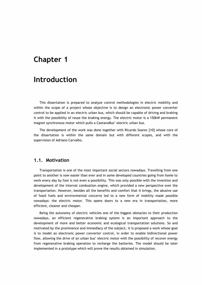
Fig 2.4 shows several topologies of converters used since the first years of development of
EPC. The circuit in a) is a buck/boost converter, which reached the operation frequency limit
in the 80’s. In order to extend the frequency range and improve its power density, it was
designed the circuit in b). However, the existence of excessive current and voltage peaks led
to the development of another topology, presented in c): ZVT (Zero Voltage Transition). After
this, it started to use “snubbers” to suppress ("snub") voltage and current transients in circuit
b) and a new topology emerged, d). To a higher boost ratio, they started to be used
topologies with coupled inductors, as shown in e). Finally, designed to be used in applications
to withstand power in the order of 100kW, the circuit in f) emerged.
10 Electrical Traction in the Power Train
Fig 2.4 – Several high efficiency switching converters’ topologies [3].
In order to improve the efficiency of the basic circuits shown before, new topologies were
designed. They are shown in Fig 2.5 and described next.
The circuit in Fig 2.5 a), “C-Bridge”, was designed to an application of 8kW and 96% of
efficiency at 25kHz of switching frequency. Later, circuit b) was obtained: “Quasiresonant
Regenerating Active Snubber (QRAS) Chopper Circuit”. It could achieve ZCS (Zero Current
Switching) at turning ON and ZVS (Zero Voltage Switching) at turning OFF and reuse the
energy of the snubber. Its efficiency is 97.5% and it was obtained for 8kW at 25kHz. This
efficiency was later improved to 98.5% using a schottky diode. The topology shown in c),
named “Snubber Assisted Zero Voltage and Zero Current Transition (SAZZ)” implements
ZVZCT (Zero-Voltage Zero-Current Transition) at turning ON and ZVS at turning OFF, using
less components than QRAS topology. It was obtained 97.8% of efficiency with 8kW at 100kHz.
The operation principle of this topology was applied to a bidirectional circuit, shown in d),
which reached 96.6% of efficiency in boost mode and 97.4% in buck mode, working with a
base power of 25kW.

Electronic Power Converters (EPC) 11
Fig 2.5 – Improved high efficiency converters topologies: unidirectional (from a to c) and bidirectional (d) [3].
2.3.2. DC/DC ZVS Bidirectional Converter with Phase-Shift + PWM
This topology consists in a DC/DC bidirectional converter, composed by a current fed half
bridge and a voltage fed half-bridge, ensuring a balance in voltage variations in the
transformer through Ca1 and Ca2 capacitors shown in Fig 2.6. Using PWM control in S1 and S2
transistors, the magnitudes of Vab and Vcd are adjusted as there are variations in the input
and output voltages, which allows to achieve ZVS in a high range of loads. The application of
Phase-Shift allows controlling the magnitude and direction of the power flow.
Fig 2.6 - DC/DC ZVS Bidirecional Converter [4].
A further analysis of this topology will not be done as it is not the aim of this document.
More information about these topologies is available in [4].
12 Electrical Traction in the Power Train
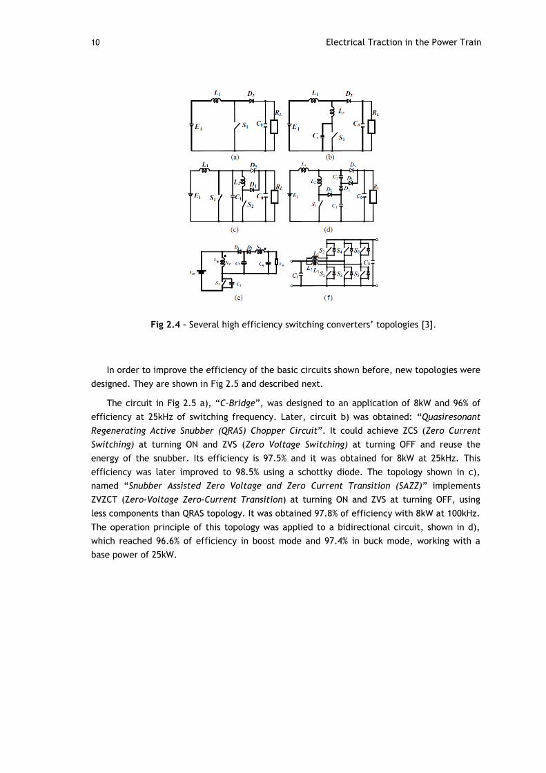
2.3.3. Improved DC/DC buck/boost Bidirectional Converter
Fig 2.7 – Improved DC/DC buck/boost bidirectional converter [5].
This converter consists in a buck/boost converter in which the inductor is divided in two,
sort of a transformer with two windings with equal number of turns. With appropriate control
it is possible to make the turns operate in parallel at the charge and in series at the
discharge, achieving a bigger step-up gain. Likewise, to buck mode, the turns operate in
series at the charge and in parallel at the discharge, achieving a bigger step-down gain. To
the same conditions, this converter has a smaller commutation current than the traditional
one [5].
There are other topologies of converters that will not be discussed in this document
because of their commonness which will not bring any added value to this document, or
because of their lack of specificity regarding the application at issue [13].
2.3.4. Isolated Full Bridge Converter
Fig 2.8 – Isolated full bridge converter.
This topology is very used in applications where bidirectional flux of energy is required
but with isolation. Having two full bridges in each side of the transformer allows more and
better types of control, permitting the usage of this topology to DC/DC, DC/AC, AC/DC and
AC/AC applications. Despite the range of possible applications, each one requires a different
and specific control. It can be either a voltage or current control, and the transistor’s signal
generation can be by hysteresis, PWM or by space vector modulation (SVM). The last one
consists in sending the signal to the transistors according to the present state of the motor

Electronic Power Converters (EPC) 13
(given by its variables) and the reference given (e.g.: State 1 -> T1 e T4 ON; T2 e T3 OFF).
More information about SVM is given in section 4.2.2.2. This topology may also be used in
three-phase applications, rather than single-phase as shown in Fig 2.8.
2.3.5. Three-phase Inverter
Considering the propose of this project, which is designing a controller for the traction of
a synchronous motor through the interface DC bus-motor, considering the freedom of control
and simplicity of the topology, a three-phase inverter will be used. It is also possible to be
used a Braking Chopper before the inverter, as shown in Fig 2.9. This chopper, composed by a
transistor and a power resistance in series, will allow the dissipation of the energy in the
form of heat if the BMS decides that the batteries could not be charged anymore and the
vehicle needs to decelerate. This heat could even be reused for the heating system of the
vehicle.
Fig 2.9 - Three-phase inverter to be used, with braking chopper and DC Link filter.
2.4. Types of Control
Motor’s control can be performed in several forms. The most common types can be
gathered in two main groups: scalar control and vector control. In permanent magnets
motors, the most used scalar control is constant V/f. However, due to the poor results
obtained in transient state, control imprecisions and phase control limitations, this type of
control is becoming less used.
To overcome the obstacles imposed by the scalar control and achieve higher
performances, vector control is adopted. Here, two main approaches are known: Direct
Torque and Flux Control (DTFC), also called Direct Torque Control (DTC), and Field-Oriented
Control (FOC). Both DTC and FOC are strategies that allow torque and flux to be decoupled
and controlled independently. Unlike FOC, in DTC there is no current loop in the control

14 Electrical Traction in the Power Train
scheme. Instead, torque and flux are measured or estimated and the control loop is closed by
the inverter’s control signals from this data [14]. Besides that, the results obtained with DTC
show that it has a better dynamic response than FOC, despite the last one having better
steady-state performance. However, DTC depends on motor parameters which, in certain
applications, is a counterpart with high relevance. [15]
Field-Oriented Control can be direct or indirect. Since there is no common agreement in
the literature in how to distinguish between them, it is assumed that indirect FOC is based on
the estimation of the flux position through stator currents and voltages and motors
parameters, whereas direct FOC measures the rotor flux position, usually by Hall sensors.
However, rotor flux cannot be sensed directly which means that some calculations must be
done after acquiring the sensor’s signal. This leads to inaccuracies, especially when the
motor’s speed is low and the stator resistance voltage drop dominates in the stator voltage
equation. It is then preferred to use a sensorless system, eliminating those inaccuracies and
providing a cheaper and more robust solution. This is the approach of the control design
developed in this work and discussed in the present document.
There are also current control strategies called Trapezoidal (Six-Step) Current Control and
Sinusoidal Current Control. These differ by the form of the current injected in the motor: the
first one tries to inject rectangular current waveforms and is usually implemented in BLDC
motors. The goal is to feed the appropriate phase of the stator in order to maintain a rotating
field. The phase shift between stator and rotor fluxes must be controlled in order to produce
the required torque. Sinusoidal Current Control is similar to the previous, except the currents
generated are sinusoidal instead of rectangular. In this type of control there is no direct
control over the torque produced making it appropriated to applications where there’s no
load variations.
In order to properly design the control over the motor, a reference frame should be
chosen. Usually the dq reference frame is chosen to apply the vector control in synchronous
machines. The dq reference frame is assumed to be rotating with an angular speed equal to
the rotor electrical angular speed (or stator rotating field angular speed, which in
synchronous machines is the same). Therefore, all the quantities represented in it are
constant at steady-state. A representation of stator voltage and current vectors as well as
rotor flux vector is shown in Fig 2.10. This situation represents a virtual motoring situation, in
which stator current vector leads the air-gap flux vector. The figure is merely representative
and intends to display the different relations between the vectors, so their modules must not
be considered.

Types of Control 15
Fig 2.10 - Representation of , and , as their dq components and angles relations at a random point of operation. Modules must not be considered.
Regarding dq frame, it is important to refer the Park Transformation, or dq0
Transformation, responsible to convert the components of a quantity (like voltage or current)
in the three-phase stationary reference frame into two-phase components in a rotating
frame. It is given by:
[
]
(2.1)
As the system is symmetric and balanced, the homopolar component given by the last line
of the matrix is not considered. So, applying the Park Transformation to the currents as an
example, the following is obtained:
[
]
[
] [
] (2.2)
Lastly, with respect to methods of electric motoring control used nowadays, five vector
control methods commonly applied to drive PMSMs are exposed, with a brief explanation of
each [15].
1. Constant Torque angle control
Torque angle is maintained at 90º turning if current component into zero.
It is used to speeds below rated speed.
Power factor decreases with the increase of rotor’s speed and stator currents.

16 Electrical Traction in the Power Train
2. Unit power factor control
Unit power factor control implies that the VA ratio of the inverter is completely
used to inject real power in the motor.
This type of control is applied controlling the torque angle as a function of
motor’s variables and is independent of motor’s speed.
The torque angle has to be higher than 90º.
3. Constant air-gap flux linkage control
The flux that results of stator current dq components and rotor flux, known as
mutual or air-gap flux, is kept constant, usually in a value that is equal to the
rotor flux.
The stator voltage requirements are kept low.
It is a simple method to apply flux-weakening, allowing the motor to operate with
speeds above the base speed.
Torque angle has to be higher than 90º.
4. Maximum Torque per Ampere control
Precious control method from machine and inverter usage point of view.
It is done controlling the torque angle.
Better performance than constant torque angle control, at the expense of higher
stator voltages.
5. Flux-Weakening control
Voltage and current limits imposed by DC bus before the inverter make the
motor’s feeding also limited. This makes the speed and torque produced by the
motor also limited. In some applications is necessary to have higher speeds than
the maxim speed permitted by the voltage and current fed to the motor
In order to increase the speed, air-gap fluxes are weakened making the
electromotive force produced by the rotor inferior to the voltage applied.
Flux-weakening is made to be inversely proportional to the stator frequency
One definition of electromagnetic torque as a function of is given by [15] and is
presented in equation (2.3).
[
( )
] (2.3)
where is the number of poles, is the d-axis inductance, is the q-axis inductance, is
the stator current vector, is the angle that stator current vector does with d-axis and is
the rotor magnetic flux.
is defined as positive to drive the motor if is positive, whereas if is negative the
torque produced is in the opposite direction of the speed, so the motor is braking. Besides
that, the two stator current components are defined as:
and .
Also, reference [15] defines as the torque angle. The author of this document gives
another definition of torque angle. This concept will be discussed in Section 4.

Types of Control 17
Through equation (2.3) it is also possible to see that if is higher than
, becomes
negative and consequently the resultant air-gap flux decreases. This is how flux-weakening
operation in permanent magnet motors is done. Furthermore, if is negative, the machine
becomes a generator. This is the main issue to the work described in this document.
2.5. Market Research
Electric and hybrid vehicles are becoming an important part of the industry nowadays.
However, they are in development stage yet and for that reason it is not easy to find many
pure electric vehicles for sale.
Concerning to the electric traction system, more specifically to regenerative braking
system, there are known two suppliers: Rexroth from Bosch group, and Continental. There
are also some electric vehicles in production that integrate this system, like Tesla, Ford,
Nissan, Mitsubishi or Renault.
2.5.1. Selling of the Regenerative Braking System
Rexoroth’s system, called Hydrostatic Regenerative Braking System (HRB), is specifically
designed to applications which, like the name indicates, are based on a hydraulic traction
system, as garbage trucks or buses. Its operation is divided in two steps: first the energy is
stored in a pressure accumulator when the vehicle brakes, converting kinetic energy into
electric energy; the energy is then restored to the transmission system, which operates
symmetrically to the step one. In order to control the charge and discharge process, and to
protect the accumulator of too much pressure, there is a set of valves that engages or
disengages this mechanism. More information about HRB is presented in [16].
Relatively to the solution provided by Continental, it is directed to any hybrid, electric or
fuel cell vehicle. When braking pedal is pressed the energy spent on the brakes is converted
in electric energy, used to charge the batteries. In addition to this brake there is a traditional
mechanical brake which is activated if the deceleration required is not enough. This decision
is made by a central controller that analyses the information from several sensors like wheel
speed, turning angle, lateral accelerations, etc. Continental also guarantees that this system,
if integrated in a vehicle with Electronic Stability Control, performs every stability functions
like ABS, TCS, etc. More information about this solution is presented in [17].
2.5.2. Electric Vehicles With Regenerative Braking
When talking about electric vehicles it is almost mandatory to talk about Tesla, the first
company to have series production of electric vehicles. Tesla started to sell electric vehicles
in a different approach: they produced an electric sport car with high performance, the
Roadster. Recently they launched another type trying to embrace other kind of buyers: the
sedan Model S. All their models (Roadster and Model S) integrate regenerative braking.
According to them, their system reuses braking energy to almost 0 Km/h, also having a

18 Electrical Traction in the Power Train
mechanism that does not let the wheels block, like ABS. It also stops regeneration if the
batteries are full charged [18].
Ford is another company that is in electric vehicles industry with Ford Focus Electric. This
car, rated as most fuel-efficient five passenger vehicle in America, also integrates
regenerative braking. Ford claim that their system regenerates up to 90% of the energy
normally lost in braking. They also say that there will be a display inside the car showing the
amount of energy being reused at each moment [19].
Nissan and Mitsubishi are in this recent market too with the same concept as Ford. Their
models, Leaf and i-Miev respectively, are city cars, small and designed to be preferentially
efficient rather than have high performances. Leaf integrates a 80kW, 280Nm motor against i-
Miev which uses a 67kW, 180Nm. Both cars are available for around 30.000€ [20].
Renault is also “in the race” with a different approach. Their vehicle, Twizy, pretends to
revolutionize the urban mobility concept. It will be available in two versions: one with a 5 CV
motor (less than 4kW) which has 45km/h of maximum speed: and another version with 20 CV
(near 15kW) that reaches 80km/h. The version with less power does not require driving
license [20].
2.6. Summary
This chapter presents the literature review within the scope of electric vehicles. First the
system overview is presented allowing a better understanding of this document purpose.
Then the requirements for the controller’s design is presented where is emphasized the
robustness of the system and the need of an auxiliary mechanical brake to assure the
vehicle’s safety. Some recent topologies of electronic power converters are presented and
briefly described, finalizing with the three-phase inverter to be used in this work. Then,
several types of control are presented and described, and the dq reference frame is
explained. It is settled that this is the reference frame to be used because in steady-state the
motor’s quantities are represented as constants. Some PMSM control methods known are then
described. Finally a market research with relation to regenerative braking system selling and
with electric vehicles in production nowadays is presented.

Chapter 3
Permanent Magnet Synchronous Motor
3.1. Introduction
With the discovery of new magnetic materials and their large availability comes the
possibility to produce new and better kinds of motor technology, making possible the
evolution in electric mobility. In an attempt to overcome the obstacles that DC motors
present, which were the most used electric motors until 1950’s, emerged the permanent
magnets synchronous motors. They do not require neither rotor windings nor external electric
sources to produce excitation in the rotor, becoming smaller, lighter and more powerful than
DC motors. They also dispense the use of brushes or slip rings, which makes them more robust
and suitable for high speed operations. Furthermore, PMSMs allow the control of their power
factor. This feature allows them to be used, for example, to make power factor correction
like capacitors.
Synchronous motors with permanent magnets are built by a rotor with permanent
magnets and a multi-phase, typically three-phase winding stator, which is fed by an external
inverter. These motors can be divided in two groups according to the type of the back
electromotive force: if it is trapezoidal one the motor is called Brushless DC (BLDC); if it is
sinusoidal it is called Permanent Magnet Synchronous Motor (PMSM), which is the object of
this thesis. Besides that, these types of motors are called synchronous because the rotor spins
at a frequency that is proportional to the rotating field created by stator currents. This leads
to the absence of slip speed which is characteristic of induction motors. The rotational force,
called torque, is achieved when the fluxes of the rotor (from the permanent magnets) and of
the stator (created by the currents) interact. It is known that when these two vectors are 90
degrees from each other, the produced torque is maximum.
In this Chapter it will be discussed the types of PMSM and their advantages and
drawbacks, how are they modeled, their operation principle and how they can be controlled,
and finally it is described the motor used in this dissertation.

20 Permanent Magnet Synchronous Motor
3.2. Types of Permanent Magnet Synchronous Motors
With respect to the direction of the flux, permanent magnets synchronous motors can be
classified as: axial flux if the air-gap flux direction is parallel to the rotor shaft or radial flux
if the air-flux direction is along the radius of the motor. Usually, axial flux motors have
advantages over radial flux motors. For the same conditions and under the purpose of the
application described in [21], axial flux motors weight less and consequently have higher
torque/mass ratio. They also can be designed to have higher power/weight ratio resulting in
less core material. They also have higher efficiency than radial flux motors [21].
Relatively to the arrangement of the permanent magnets, they can be: surface (SPM),
surface inset or interior mounted (IPM). Surface mounted permanent magnets motors have
the highest air gap flux density but lower structural integrity and robustness. Because of this
they are not used in applications that require operating speeds above 3000 rpm. Since the
permanent magnets permeability is close to the air permeability, the rotor is isotropic. The
interior mounted types of motors are the most robust which makes them preferential to very
high speed applications. Surface inset rotors are like SPM but they have an iron tooth
between each couple of adjacent PMs. This leads to a slight anisotropy which, in turn, leads
to the existence of two torque components: the permanent magnet torque and the
reluctance torque. Interior mounted rotors have several flux barriers per pole, as shown in
Fig 3.1. In this case, the rotor has three flux barriers per pole. Higher number of flux barriers
per pole leads to higher rotor anisotropy. Here, the torque reluctance component is higher,
hence the IPM rotor exhibits a high torque density and it is well-suited for flux-weakening
operations, up to very high speeds.
Fig 3.1 – Rotor arrangements of PMSM: a) surface mounted (SPM), b) inset surface mounted and c) interior mounted (IPM) [6].
Types of Permanent Magnet Synchronous Motors 21
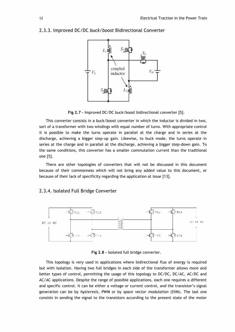
Even on the subject of IPMs, they can be distinguished according to the direction of the
magnetization of the PMs as: Tangentially magnetized and radially magnetized. An
illustration of both types is shown in Fig 3.2. Tangentially magnetized rotors create an air gap
flux as the sum of two adjacent magnets. In radially magnetized rotors, the PM surface is
lower than the pole surface, yielding a lower flux density in the air gap. This configuration
can be designed with more than one barrier per pole, which leads to high anisotropy. In both
configurations the magnets have alternating polarity. IPM motors have magnetic paths with
different permeability, through which is possible to develop a reluctance torque.
Fig 3.2 – IPM rotor with four poles with a) tangentially magnetized PMs and b) radially magnetized PMs [6].
From the stator windings point of view, as the rotor rotates the magnetic reluctance
varies continuously. It changes between two extreme values: the maximum along the d-axis
and the minimum along the q-axis. So, two corresponding winding self-inductances can be
defined as the minim inductance and the maximum.
and are two important parameters of the motor because they are used in motor
model equations in order to achieve a proper control – this will be discussed on the next
chapter. These inductances depend on the air-gap of flux paths. As said before, the
permeability of the magnets are low and approximately the same as the permeability of the
air. Thus, SPM motors have and one can consider that the air-gap thickness is bigger
in this case. Similarly, in IPM motors the PM’s have lower permeability that the iron (that is,
higher reluctance) so the effective air-gap in the magnetic flux path varies according to rotor
position. In this case the resulting d-axis inductance is lower than q-axis inductance, yielding
. Also, the saliency ratio (or anisotropy ratio) is defined as
.
The phase inductance of the motor can be calculated from and through equation
(3.1). As shown, the self-inductance of each phase can be position independent only if and
are the same, for example in SPM motors [6].
( )
[
( )
] (3.1)

22 Permanent Magnet Synchronous Motor
where is the instantaneous position of the rotor d-axis with respect to one phase. For
simplicity usually phase “a” is considered.
The concept of magnetic flux paths and d and q inductances are better understood
through the representation presented in Fig 3.3.
Fig 3.3 – Magnetic flux paths in a) SPM motor and b) IPM motor [7].
3.3. PMSM Modeling
In order to accomplish a simpler way to model the PMSM, the dq reference frame is
adopted. That is because the dq frame is rotational with an angular speed equal to the
electrical angular speed, that is
, where is the number of poles and is the
mechanical angular speed of the shaft. Two reference frames can be chosen: stator and rotor
reference frame. For simplicity, the rotor reference frame is adopted. The principle of this
model assumes that the rotor flux is aligned with the d-axis, while q-axis is in quadrature -
that is leading by 90 electrical degrees. This way there is no rotor flux along q-axis. It is also
assumed that the motor’s core losses are negligible, so are the magnets fluxes variations due
to temperature variations. A representation of the dq axis in a four-pole IPM rotor can be
found in Fig 3.2.
However, it is essential to understand where the dq frame comes from. First of all, PMSM
is a three-phase machine which is supposed to be balanced, so currents and voltages are 120º
from each other. It is much simpler to work on an orthogonal two-phase referential. That
transformation is accomplished applying the Clarke-Transformation to the three-phase units
as shown in equation (3.2).
[
]
[
√
√
]
[
] (3.2)
where could be voltage, current or any other three-phase unit.
The result is a two-phase orthogonal frame called Alpha-Beta (αβ) frame. The Clarke-
Transformation can also be found in a power invariant form, which has a √ ⁄ multiplying
factor instead of ⁄ .
PMSM Modeling 23
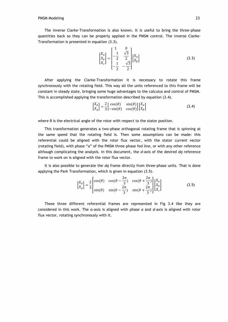
The inverse Clarke-Transformation is also known. It is useful to bring the three-phase
quantities back so they can be properly applied in the PMSM control. The inverse Clarke-
Transformation is presented in equation (3.3).
[
]
[
√
√
]
[
] (3.3)
After applying the Clarke-Transformation it is necessary to rotate this frame
synchronously with the rotating field. This way all the units referenced to this frame will be
constant in steady state, bringing some huge advantages to the calculus and control of PMSM.
This is accomplished applying the transformation described by equation (3.4).
[
]
[
] [
] (3.4)
where θ is the electrical angle of the rotor with respect to the stator position.
This transformation generates a two-phase orthogonal rotating frame that is spinning at
the same speed that the rotating field is. Then some assumptions can be made: this
referential could be aligned with the rotor flux vector, with the stator current vector
(rotating field), with phase “a” of the PMSM three-phase fed line, or with any other reference
although complicating the analysis. In this document, the d-axis of the desired dq reference
frame to work on is aligned with the rotor flux vector.
It is also possible to generate the dq frame directly from three-phase units. That is done
applying the Park Transformation, which is given in equation (3.5).
[
]
[
] [
] (3.5)
These three different referential frames are represented in Fig 3.4 like they are
considered in this work. The α-axis is aligned with phase a and d-axis is aligned with rotor
flux vector, rotating synchronously with it.

24 Permanent Magnet Synchronous Motor
Fig 3.4 – Representation of the three reference frames: three-phase, dq and αβ. d-axis aligned with rotor flux. α-axis aligned with phase-a.
The motor modeling is now ready to be done, assuming that dq frame is used from now on
as reference. Therefore, the PMSM stator equations referenced to rotor are represented in
equation (3.6).
{
(3.6)
{
(3.7)
where is the stator phase resistance, is the stator current vector, is the differential
operator, is the flux, is the rotor flux, is the electrical angular speed, is the
inductance, the subscript refers to the stator and d and q refers to direct and quadrature
axis, respectively.
As the permeability of high flux density permanent magnets is almost the same of the air,
the magnetic thickness becomes an extension of the air gap by that amount. Then, the stator
inductance when the stator winding is aligned with the magnets is called the direct axis
inductance ( ). By rotating the magnets by 90 electrical degrees, the stator flux sees the
area of the rotor which contains only the iron path. The inductance measured there is called
quadrature axis inductance ( ). The direct axis reluctance is greater than the quadrature
axis reluctance [15]. This results in an unequal relation between and given by .
The equation (3.6) can be represented in two electric circuits as shown in Fig 3.5.

PMSM Modeling 25
Fig 3.5 – d and q representation circuits of a PMSM.
As shown, the rotor flux is all along the d-axis which produces an EMF along the q-axis.
This is an important assumption when talking about the control of PMSM, later on this
document.
Now it is possible to define the electromagnetic torque expression as a function of flux
and current dq components. The equation is represented in (3.8).
( ) (3.8)
where is the number of poles of the PMSM.
This expression states essentially two things: first, that there is a component that is
directly proportional to the torque produced and other that is against the torque. This allows
renaming the dq current components for better and easier understanding the rest of this
document: is the Torque-producing component and is the Flux-producing component;
Second, that the electromagnetic torque is defined by the cross product between flux and
current vector, which means that the d component of one is multiplied by the q component
of the other. This allows re-writing the electromagnetic torque expression as in equation
(3.9). It is easy to see that is maximum when the angle between current and air-gap flux
vectors is 90 degrees.
| || | (3.9)
where is the stator current vector (responsible for the rotating field), is the air-gap flux
vector (resultant of the rotor flux and stator induced flux) and is the torque angle.
Also, using the relations defined in (3.7) it is possible to unfold equation (3.8) in two
components: the fundamental torque component due to the permanent magnets flux
multiplied by the torque-producing current component, and the reluctance torque
component due to the difference between d and q inductances multiplied by both dq current
components. This equation is presented in (3.10).
[ ] (3.10)

26 Permanent Magnet Synchronous Motor
3.4. Definitions of Torque Angle
The latter equation (3.9) leads this document to a very important concept in this subject:
the definition of torque angle. Unfortunately, literature is not consistent in what is, in fact,
the torque angle. Many definitions are given for the same angle, and many different angles
are defined as the same thing depending on the author. Being aware of this is, of course, a
huge problem because it makes impossible to do a quick review of an article without reading
the context in which it is inserted and the definitions that the author does. Furthermore,
achieving a correct vector control over the motor implies the knowledge of which angle is
being taking into account in each case which, in turn, inevitably implies their correct
differentiation and definition.
A relevant definition is given in [15] by R. Krishnan. He claims that the torque angle is the
angle between stator current vector and rotor flux vector. In fact, this consideration is valid
because the electromagnetic torque is still defined as the interaction between two magnetic
forces, one created only by the stator current and other created only by the rotor’s
permanent magnets. This consideration allows re-writing the torque equation as (2.3)
presented in Chapter 2.4 and repeated here for convenience.
[
] (3.11)
Now is easy to understand the definitions of dq current components given by Mr. Krishnan
and considered valid by the author of this dissertation: being the torque component and
being the flux component. In dq reference frame is the projection of over the d-axis
( ) and is the projection of the same vector over the q-axis ( ). So the
interaction between stator current torque component and rotor flux creates torque, and all
the considerations become valid. Moreover, another noteworthy aspect is that for SPM motors
and are equal, making the second portion of the equation null, thus controlling the
motor’s torque only by the influence of From now on the angle is considered to be the
stator current angle.
Another important reference to this issue is made by Mr. Wilamowski [6]. In this book two
different angles are called “torque angle”. One is the angle between rotor flux vector and
stator current vector (the same as before), and the other one is the angle between rotor and
stator flux vectors, which is called from now on as . The second vector is in fact the air-gap
flux vector and this is concluded because of the definitions given in the same book. The
author claims that the first angle definition is used in FOC algorithms and the second one in
DTC techniques. However, this angle has a direct relation with the stator current angle ,
allowing its usage in another control strategy than DTC. Their relation is given by the
definitions of stator current and air-gap flux vectors in dq reference frame. Considering the
relations shown in (3.12) and (3.13) it is possible to conclude the relations shown in (3.14)
and (3.15).
(3.12)
(3.13)

Definitions of Torque Angle 27
(3.14)
(3.15)
Lastly there is another definition that is quite different from the previous. The approach
of the author is in a more physical and mechanical way, concerning the synchronous
electrical machines functionality [22]. The torque angle , defined in Chapter 2.11 of the
mentioned book, is stated to be the angle between the phase voltage and a virtual – as
corresponding to running of the motor without stator supply - voltage defined as the effect of
the rotor’s magnetomotive force (MMF), . The stator current also creates a flux aligned
with it, which induces a voltage lagging by 90º, . The air-gap flux is considered to induce a
voltage on the stator, called , which is given as the sum of two other virtual voltages:
and . So, if the stator resistance is neglected, as well as all the losses of the motor, then
the power that feds it must be equal to the power generated. Therefore, if this power per
phase is defined as the product of line voltage and current times the angle between them
(power factor) as in equation (3.16), and the phase reactance, called synchronous reactance
( ) and defined as the sum of the magnetizing reactance with the leakage reactance, is
given, then the torque can be expressed as in equation (3.17).
| || | (3.16)
| | | |
(3.17)
This approach could be valid in a control implementation and a technique based on it is
tested to achieve sensorless operation. However, no good results were obtained. The
technique is based on the power balance and is described in Section 4.5.
The author of this dissertation considers the definition of torque angle as the angle
between stator current vector and air-gap flux vector, as described in equation (3.9). This
consideration is because of the physical behavior of the PMSM. Considering that the
electromagnetic torque is created by the interaction between two magnetic fields, it makes
perfect sense that it is defined by the multiplication of the module of the vector that
represents the stator current – responsible for creating a magnetic field aligned with itself,
the module of the vector that represents the air-gap flux – the resultant flux of the
interaction between stator and rotor fluxes, and the angle between them. Therefore, when
stator current vector is leading air-gap flux by 90º the maximum torque is achieved. This
torque angle definition is adopted from now on.
All these relations are graphically represented in Fig 2.10.

28 Permanent Magnet Synchronous Motor
3.5. Relations Between Torque Angle, Current and Air-gap Flux
The next conclusions are useful for better understanding the PMSM behavior with respect
to air-gap flux and stator current vectors’ variations.
Starting from equation (3.9) some conclusions are drawn with respect to the influence of
variations in one vector in relation to the others, considering constant torque, that is
. Therefore, three situations are possible to analyze: current variations, air-gap flux
variations and position variations. However, the next analysis is merely theoretical because a
complete decoupling of the vectors in question is impossible.
The equation (3.18) is intended to be analyzed. It is the result of deriving equation (3.9)
considering constant . To do that, the derivative rule defined by is used.
[| || | ] (3.18)
(3.19)
3.5.1. Torque dependability on | | and | |
Since variations in imply variations in - because the definition of the latter includes
the two components of the first – these two conditions are analyzed together. Solving (3.19)
in order to leads to equation (3.20).
(3.20)
From this equation it is possible to conclude that with the increase of there should be a
subsequent decrease of and/or . Decreasing means that the angle between both
vectors becomes smaller, meaning that the vectors move closer to each other. This analysis
makes sense since theoretically the torque is maximum when both vectors are 90º from each
other. If the first consideration for this analysis is that torque is constant, then if there is an
increase in stator current, either air-gap flux decreases or the vectors come closer to each
other. Since it is physically impossible to decouple and vectors this conclusion is
consistent with physical phenomena.
Moreover it is possible to analyze motor’s behavior in two distinct conditions: 1) when
and 2) when ∧ .
The first condition is when causes the same variations in both current and air-gap flux
vectors. This corresponds to the generic conclusion drawn before.
The second condition has two possible behaviors according to the variations in . If it
increases then also increases but decreases. In the other hand, if decreases also
decreases but increases. This is the only situation in which those two vectors have
symmetrical behaviors.

Relations Between Torque Angle, Current and Air-gap Flux 29
3.5.2. Torque dependability on
Controlling is perhaps the most appropriate way of controlling the torque in a PMSM.
If, somehow, it was possible to directly extract this angle information from the motor, its
variations will directly correspond to variations in torque, allowing the control of the motor.
However, for extracting it is first needed to know current and flux vectors, which makes
this approach of control difficult to implement.
Through the analysis of the same equation it is possible to conclude what have been said.
For constant torque, if a variation in occurred, air-gap flux and stator current have to
compensate by changing their amplitudes.
3.6. Used Motor’s Parameters and Simulation
The nominal values and the parameters of the motor that is used in simulation tests are
described in Table 3.1 and in Table 3.2, respectively. As said before, this motor is smaller
than the CaetanoBus’ and its purpose is to test the designed control.
Table 3.1 – Nominal values of the PMSM used in simulation.
Connection Y
Number of poles 4
Rated Current 160A
Rated frequency 200Hz
Rated power 50kW
Rated torque 80Nm
Table 3.2 – Parameters of the PMSM used in simulation.
Stator Resistance 7.9mΩ
d-axis Inductance 0.23mH
q-axis Inductance 0.56mH
Rotor flux 104mWb
A model of the motor is built based on the equations described before. Using the PSIM
ability of running a DLL file through the DLL Block, and using Microsoft Visual C++ 2012
Express software, the model was programmed in C++ code and tested in PSIM.
A simulation for testing the model is done as shown in Fig 3.6. The inverter, on the left
side of the figure, is controlled in open-loop by a sine-PWM signal generator. Then, the three-
phase voltages are transformed in dq voltages through Park Transformation, as explained
before, and feed the motor. All the parameters of the motor are established outside the
model allowing their modification without the need of changing the code. Moreover, the load
torque ( ) is also available for changing outside the model by a step voltage source, allowing
the introduction of a load torque at any instant. The motor’s dq current components are used
as feed-back to calculate the torque, and the rotor angular speed is converted in electrical

30 Permanent Magnet Synchronous Motor
angular speed and integrated, so the position of the rotor could be used in Park
Transformation.
Fig 3.6 – DLL model of PMSM in PSIM software.
Building this model allow the validation of system’s equations as well as a better
understanding of its behavior and familiarization with PSIM software. However, from this
point on, the PMSM block and Park Transformation block of PSIM are used since they satisfy
the requirements for this work.
3.7. Summary
A detailed analysis of the permanent magnet synchronous motor is presented in this
chapter. Several architectures of PMSMs are presented with respect to permanent magnets
arrangement. Then, its mathematical model in dq reference frame is presented and
explained, with the relations between three different reference frames. An important
analysis to the different definitions of torque angle presented in literature is done, describing
each one and assuming for this document purposes that torque angle is between stator
current and air-gap flux vectors. A dynamic analysis of torque dependability on stator current
and air-gap flux vectors is presented, finalizing with the description of the motor used for
this work and its PSIM model created. A DLL model is chosen allowing its designing in C++
language.
Chapter 4
Control of the PMSM
4.1. Introduction
Although making a PMSM to run is not a hard task to do, controlling it is not trivial. In the
literature several strategies of control are presented. There are roughly two ways of
controlling a motor: scalar and vector control. Vector control allows better control over the
behavior of the motor since all its variables are considered (voltage, currents, fluxes, position
and speed). This document studies, analyses and compares three methods of vector control:
Stator current vector at 90 degrees, Air-gap flux vector at 90 degrees and Maximum Torque
Per Ampere (MTPA). These three methods have different characteristics regarding dynamic
response and controllability, but particularly with regard to efficiency, which is important
considering that the motor is fed by batteries.
Beyond the control methods there is the inverter control technique, which generates the
gate signals for the transistors. This could be by Hysteresis, Sinusoidal Pulse-Width
Modulation (PWM) or by Space Vector Modulation (SVM). Only the last two have been analyzed
and compared due to goals of the work.
In this context, the used controller type must also be considered. Among various types of
controllers that are used nowadays, such as PID, Fuzzy, Neuronal-Networks, Sliding-Mode or
Adaptive control, only PID is used in this work. Although its performance cannot be the best
one, it is linear, simpler and faster to implement than the others and requires less processor
usage. This last characteristic is very important since the application of the controller is in an
electric vehicle, where robustness and fast response are critical.
Last but not least, two control platforms are analyzed: DSP and FPGA. Although the
control of the system is not yet implemented, it is the final objective. Therefore, a study of
these two controller platforms is conducted. The performed analysis could be used in future
works with respect to this subject.
This Chapter describes each type of control mentioned above, analyses them
comparatively and shows the simulation results.

32 Control of the PMSM
4.2. Control Strategy
Unlike most of the literature already studied, it is implemented a torque control scheme.
In this strategy a torque reference is given to the motor, instead of a speed reference as is
typically used. This makes a huge difference when the purpose of the system is an electric
vehicle application. In this case, it is possible to say that it is the driver who “closes the
speed loop” of the control. In other words, the motor accelerates and decelerates according
to the torque supplied by the acceleration (or braking) pedal. It is driver’s job to choose if he
wants to go faster or slower, and that information is given to the motor by a torque reference
as it is done in ICE vehicles. This concept intrinsically avoids the loss of synchronism, one of
the biggest problems of controlling this kind of motors. This assumption can be proved by
mechanical electromagnetic torque equation as in (4.1).
(4.1)
where is the load torque, is the moment of inertia, is the friction coefficient and is
the angular speed of the shaft.
Through this equation it is possible to understand that when the motor receives a torque
reference (admitting that it can effectively produce that torque) any disturbance to the
system will affect only the speed. Once again, if the speed loop of the controller is closed by
the driver, he must respond to that disturbance applying more or less torque reference. If the
reference of the controller had been speed, at any instant, if there was any disturbance and
the torque is already maximum, the motor would lose synchronism, which could lead to
system failure. This assumption can be proved by the torque analysis made on Chapter 3 and
summarized here: if no more current can be drawn from the source then the current vector is
maximum, so it is the air-gap flux vector. The angle between them, torque angle, is then 90º.
If any disturbance occurs, like a road bump or some kind of road cavity, then the rotor will be
held back and there will be no more power to pull it over again, resulting in the loss of
synchronism. Considering the operation with a position sensor, this situation could possibly be
predicted and corrected. But with a sensorless system, like it is proposed in this work, that
loss of synchronism could be fatal.
Three methods of control are to be discussed: Stator current ( ) at 90 degrees, air-gap
flux ( ) at 90 degrees and Maximum Torque Per Ampere. These three methods, although
being based on the same concept, have different dynamic responses and are designed under
different considerations.
4.2.1. Control Methods
The approach used to control the PMSM is based on a torque reference control. That
reference is compared with the calculated motor torque and the error is then brought to zero
with a PI which gives the reference. Through system of equations (3.6), voltage
reference is obtained. At the same time, is calculated by one of the methods described
next. voltage is then obtained in the same way that , and Park-Transformation is
applied to generate phase reference voltages, , , and , using the rotor

Control Methods 33
position signal that comes from the integration of a speed sensor signal. It is important to say
that in fact there is a coupling between d and q components (voltages and currents), which
means that it is not possible to generate them separately, being one dependent on the other.
Therefore, they must be generated simultaneously.
Through equation (3.9) it is clear that the produced torque is maximum when stator
current vector is leading air-gap flux vector by 90º. Moreover, for regenerative braking mode,
the torque must be negative so being in opposite direction of the speed, working as a
generator. This means that the stator current vector becomes lagging the air-gap flux vector,
thus making torque angle negative. In the control strategy described, a negative torque
reference is given (by vehicle’s braking pedal) which produces a negative reference. The
relations between various vectors and their dq components are shown in Fig 2.10.
As discussed in Chapter 3 the torque equation can be written as a function of as in
(3.11). This equation will be analyzed and used in MTPA method discussed on Chapter
4.2.1.3.
4.2.1.1. Stator Current ( ) Vector at 90 Degrees
In this method, vector is maintained at 90 degrees from the rotor flux vector (which is
aligned with d-axis). That way the d- component of is zero. That means is controlled only
by . This virtually eliminates the dq coupling issue talked before. The torque expression
given in (3.10) becomes:
(4.2)
and torque per stator current is constant and equal to
.
Normalized electromagnetic torque is then given by:
(4.3)
where the subscript means normalized.
As shown in (4.2), in this control method, torque is controlled by and directly
proportional to . Also, and are equal in p.u., making it the simplest method. Motor’s
equations from (3.6), in steady state become those as shown in system of equations (4.4).
{
(4.4)
However, this method has some issues concerning power factor. It can be seen from Fig
2.10 that power factor can be calculated by equation (4.5) [15].
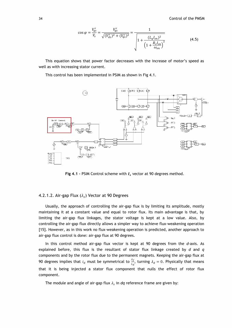
34 Control of the PMSM
√
√
(
)
(4.5)
This equation shows that power factor decreases with the increase of motor’s speed as
well as with increasing stator current.
This control has been implemented in PSIM as shown in Fig 4.1.
Fig 4.1 - PSIM Control scheme with vector at 90 degrees method.
4.2.1.2. Air-gap Flux ( ) Vector at 90 Degrees
Usually, the approach of controlling the air-gap flux is by limiting its amplitude, mostly
maintaining it at a constant value and equal to rotor flux. Its main advantage is that, by
limiting the air-gap flux linkages, the stator voltage is kept at a low value. Also, by
controlling the air-gap flux directly allows a simpler way to achieve flux-weakening operation
[15]. However, as in this work no flux-weakening operation is predicted, another approach to
air-gap flux control is done: air-gap flux at 90 degrees.
In this control method air-gap flux vector is kept at 90 degrees from the d-axis. As
explained before, this flux is the resultant of stator flux linkage created by d and q
components and by the rotor flux due to the permanent magnets. Keeping the air-gap flux at
90 degrees implies that must be symmetrical to
, turning . Physically that means
that it is being injected a stator flux component that nulls the effect of rotor flux
component.
The module and angle of air-gap flux in dq reference frame are given by:

Control Methods 35
| | √
√
(4.6)
(4.7)
This control has been implemented in PSIM as shown in Fig 4.2.
Fig 4.2 - PSIM Control scheme with at 90 degrees method.
4.2.1.3. Maximum Torque Per Ampere (MTPA)
This method pretends to achieve the best performance results with respect to battery
efficiency. The goal is to produce maximum electromagnetic torque with the less current
possible. This has repercussions in the voltage required by the inverter. However, in this
application, is preferred to have less current than less voltage to the same torque produced.
The mathematical principle behind this method is implicit in its own name. It is necessary
to reach a torque per ampere equation and then derive it and equate it to zero to find its
maximum or minimum. This last consideration is done evaluating the physical operation of
the machine after well understanding its behavior.
Through equation (3.11) it is possible to write an equation in function of torque per
ampere as in (4.8).
(
) (4.8)
Deriving this equation with respect to , and equate it to zero gives:
( ) (4.9)
where .
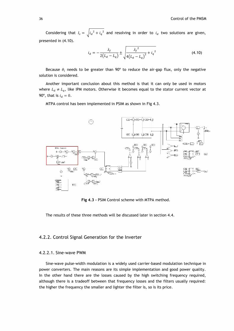
36 Control of the PMSM
Considering that √
and resolving in order to two solutions are given,
presented in (4.10).
( ) √
( )
(4.10)
Because needs to be greater than 90º to reduce the air-gap flux, only the negative
solution is considered.
Another important conclusion about this method is that it can only be used in motors
where , like IPM motors. Otherwise it becomes equal to the stator current vector at
90º, that is .
MTPA control has been implemented in PSIM as shown in Fig 4.3.
Fig 4.3 - PSIM Control scheme with MTPA method.
The results of these three methods will be discussed later in section 4.4.
4.2.2. Control Signal Generation for the Inverter
4.2.2.1. Sine-wave PWM
Sine-wave pulse-width modulation is a widely used carrier-based modulation technique in
power converters. The main reasons are its simple implementation and good power quality.
In the other hand there are the losses caused by the high switching frequency required,
although there is a tradeoff between that frequency losses and the filters usually required:
the higher the frequency the smaller and lighter the filter is, so is its price.
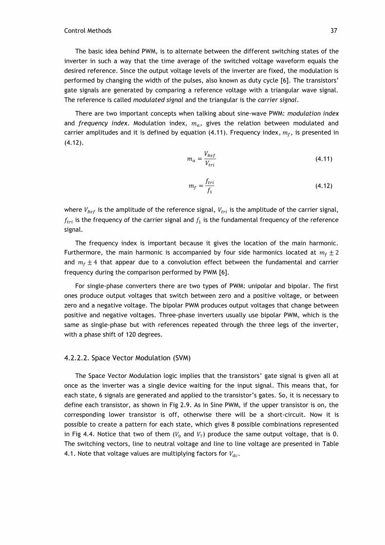
Control Methods 37
The basic idea behind PWM, is to alternate between the different switching states of the
inverter in such a way that the time average of the switched voltage waveform equals the
desired reference. Since the output voltage levels of the inverter are fixed, the modulation is
performed by changing the width of the pulses, also known as duty cycle [6]. The transistors’
gate signals are generated by comparing a reference voltage with a triangular wave signal.
The reference is called modulated signal and the triangular is the carrier signal.
There are two important concepts when talking about sine-wave PWM: modulation index
and frequency index. Modulation index, , gives the relation between modulated and
carrier amplitudes and it is defined by equation (4.11). Frequency index, , is presented in
(4.12).
(4.11)
(4.12)
where is the amplitude of the reference signal, is the amplitude of the carrier signal,
is the frequency of the carrier signal and is the fundamental frequency of the reference
signal.
The frequency index is important because it gives the location of the main harmonic.
Furthermore, the main harmonic is accompanied by four side harmonics located at
and that appear due to a convolution effect between the fundamental and carrier
frequency during the comparison performed by PWM [6].
For single-phase converters there are two types of PWM: unipolar and bipolar. The first
ones produce output voltages that switch between zero and a positive voltage, or between
zero and a negative voltage. The bipolar PWM produces output voltages that change between
positive and negative voltages. Three-phase inverters usually use bipolar PWM, which is the
same as single-phase but with references repeated through the three legs of the inverter,
with a phase shift of 120 degrees.
4.2.2.2. Space Vector Modulation (SVM)
The Space Vector Modulation logic implies that the transistors’ gate signal is given all at
once as the inverter was a single device waiting for the input signal. This means that, for
each state, 6 signals are generated and applied to the transistor’s gates. So, it is necessary to
define each transistor, as shown in Fig 2.9. As in Sine PWM, if the upper transistor is on, the
corresponding lower transistor is off, otherwise there will be a short-circuit. Now it is
possible to create a pattern for each state, which gives 8 possible combinations represented
in Fig 4.4. Notice that two of them ( and ) produce the same output voltage, that is 0.
The switching vectors, line to neutral voltage and line to line voltage are presented in Table
4.1. Note that voltage values are multiplying factors for .
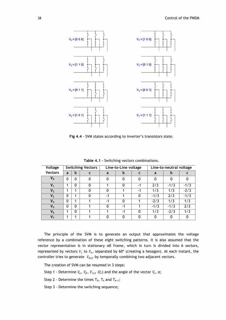
38 Control of the PMSM
Fig 4.4 - SVM states according to inverter’s transistors state.
Table 4.1 – Switching vectors combinations.
Voltage
Vectors
Switching Vectors Line-to-Line voltage Line-to-neutral voltage
a b c a b c a b c
V0 0 0 0 0 0 0 0 0 0
V1 1 0 0 1 0 -1 2/3 -1/3 -1/3
V2 1 1 0 0 1 -1 1/3 1/3 -2/3
V3 0 1 0 -1 1 0 -1/3 2/3 -1/3
V4 0 1 1 -1 0 1 -2/3 1/3 1/3
V5 0 0 1 0 -1 1 -1/3 -1/3 2/3
V6 1 0 1 1 -1 0 1/3 -2/3 1/3
V7 1 1 1 0 0 0 0 0 0
The principle of the SVM is to generate an output that approximates the voltage
reference by a combination of these eight switching patterns. It is also assumed that the
vector representation is in stationary αβ frame, which in turn is divided into 6 sectors,
represented by vectors to , separated by 60º (creating a hexagon). At each instant, the
controller tries to generate by temporally combining two adjacent vectors.
The creation of SVM can be resumed in 3 steps:
Step 1 - Determine , , ( ) and the angle of the vector , α;
Step 2 - Determine the times T0, Tk and Tk+1;
Step 3 - Determine the switching sequence;
Control Methods 39
Step 1
and are determined using the Clarke Transformation, explained in the previous
chapter. Then, √
and
. Comparing with 6 different angles given by
the vectors to , the Sector of is known.
Step 2
,
and
represent the duty cycle of each vector , being the modulation period.
and are given in [6] by:
| |
{
√ } (4.13)
| |
√ (4.14)
(4.15)
Step 3
The switching pattern chosen can be either with 7 or 5 segments. The difference is
whether or not one uses both zero vectors ( and ). In terms of output voltage, they are
the same. So, for simplicity, and for reduce the number of commutations, it is used the 5
segments technique. Furthermore, as said before, vectors and produce the same output
voltage so either one can be chosen knowing that:
For the following relations hold:
- The phase c component of all vectors generated in sector 1 and 2 is always 0.
- The phase a component of all vectors generated in sector 3 and 4 is always 0.
- The phase b component of all vectors generated in sector 5 and 6 is always 0.
In the same way, for the following relations hold:
- The phase a component of all vectors generated in sector 6 and 1 is always 1.
- The phase b component of all vectors generated in sector 2 and 3 is always 1.
- The phase c component of all vectors generated in sector 4 and 5 is always 1.
Once again to keep it simple, is chosen.
The sequences are different if it is considered odd or even sectors. That is because it is
intended to maintain the pattern symmetrical to the center of . Therefore, the sequences
are shown in Fig 4.5 and Fig 4.6 [6].

40 Control of the PMSM
Fig 4.5 - SVM sequence for odd sector.
Fig 4.6 - SVM sequence for even sector.
Finally the tables containing the transistors’ firing sequences have to be built. There
should be one table for each transistor and they should be built considering a sector for each
row and the sequence shown above for the columns. The value of each cell is selected
making the correspondence between the Sector, the segment and the corresponding
transistor signal given by Table 4.1. Notice that tables for transistors 4, 6 and 2 are
complementary of tables 1, 3 and 5 respectively. The following table is an example for
transistor T1:
Table 4.2 – Example of a SVM table for transistor T1.
Segment 1 Segment 2 Segment 3 Segment 4 Segment 5
Sector 1 0 1 1 1 0
Sector 2 0 0 1 0 0
Sector 3 0 0 0 0 0
Sector 4 0 0 0 0 0
Sector 5 0 0 1 0 0
Sector 6 0 1 1 1 0
The implementation of SVM in PSIM can be seen in Fig 4.7. The steps described before are
highlighted for easier understanding of the model.
Fig 4.7 – SVM model designed in PSIM with different steps highlighted.
Control Methods 41
4.2.3. Controllers’ Tuning
At this point three methods of control were described as well as two signal generation
techniques for the inverter. In this section a brief overview over nowadays most used
controller types is done and the PI controllers used for this work are explained. Several
controller types are known but the most used are PID (Proportional-Integral-Derivative) or
variances like PI, PD, PI+D, etc., Fuzzy Logic or variances like Adaptive-Fuzzy Logic, Artificial
Neural Networks (ANN) of variances like Neuro-Fuzzy Networks, and Genetic Algorithms.
Although PID controllers have a general application capability they often do not provide
an optimal control. The main reason is because they consist in a feedback system, with
constant parameters and without any knowledge of the process. Furthermore, in applications
where there is no possibility of having overshoot, like some industry machinery, the gains
should be small resulting in poor performance.
Despite this, and considering the requirements of the system, only PID controllers are
object of evaluation in this work. That is because of its simplicity and linearity, which
simplifies its implementation and turns the control program faster. If the tests conducted
with this controller result in a satisfactory performance, the usage of other type of controller
is disregarded. Otherwise some more comparison tests should be done in order to evaluate
the controller that has the best trade-off between performance, robustness and
computational demand.
PID mechanism consists in minimizing the error between a reference value and a
measured output of a process by feedback. Mathematically the controller is a sum of a gain,
integration and derivation of the error at its input. Heuristically these three values can be
understood with respect to time: proportional (P) depends on the present error, integral (I)
depends on past errors and derivative (D) predicts future errors. By tuning these parameters
through their gains (Kp, Ki and Kd, respectively) it is possible to adjust the dynamic and
steady-state response of the controller as wish. So, two main approaches are considered: one
called regulation whose objective is to stay at a given set point, rejecting any disturbances;
and other named command tracking which has the objective to perfectly follow (track) the
changes in the given reference. Some processes demand one of these approaches while
others must be settle with the other. In this case, in which the process is a PMSM vehicle, a
balance between them is required because the reference is constantly changing and
disturbances are expected to happen. So, this means that there must be a trade-off between
the results obtained. Probably a very quick response would have some overshoot and ringing
of the signal. No-overshoot and smooth response would be accomplished as a cost of slower
response. Moreover, PID controller is typically only used when the process is a second-order
one. For simpler systems the derivative component is not considered. Another reason for the
absence of the derivative component is the amplification of noise. Any peaks in the input
signal of the controller would lead to huge outputs by the derivative gain which would then
be accumulated be the integral gain, and the system remains unstable and uncontrollable.
Therefore, PI controller is usually used in slower and single-order systems. This is the case of
this work, where the largest time constant of the system is defined by the shaft constant of
the motor as
, where is the moment of inertia and is the friction coefficient. In the
frequency domain it causes the dominant pole, which is the pole that dictates the slower

42 Control of the PMSM
time response of the system, giving the information of “how fast” should the controller be to
have good performance.
The output of a PID controller can be expressed in time domain as:
∫
(4.16)
where ,
and are the proportional, integral and derivative gains
respectively, and is the input error signal. and are the integrative and derivative
time constants, respectively.
In the frequency domain PID is known for its Laplace form:
(4.17)
4.2.3.1. PI Controller Tuning
There are several methods to tune a PI controller. Although most sophisticated
techniques are subject of patents and used in simulations software, there are some simpler
forms of tuning the PID controllers. The most common ones are: Ziegler-Nichols, Software
tools and Manual Tuning. Ziegler-Nichols method is as experience based technique and
although it was designed for PIDs, it can be used for PIs and even P controllers. Its procedure
goes like this: I and D gains are started as zero and the P gain is increased until the process
starts to oscillate, Kmax. The period of the oscillation is recorded, Pu. Then, for the controller
type chosen, one of the lines of Table 4.3 is chosen and their gains are applied.
Table 4.3 – Ziegler-Nichols method.
Control Type
P 0.5Kmax - -
PI 0.45Kmax 1.2Kp/Pu -
PID 0.6Kmax 2Kp/Pu KpPu/8
Many software tools are available for tuning PIDs. They usually require the mathematical
model of the process and some other controller parameters so an Auto-tune can be
performed. In Simulink, for example, there is a toolbox (SiSoTool) that allows the user to
design the controller as wish. The response to several types of input can be seen and the
adjustments can be done in real-time. However, some advanced control skills are needed to
achieve good results without consuming large amounts of time.
The first approach to the PIs tuning for this work was done in Simulink as described
before. A model of the process was built and SiSoTool toolbox was used to tune the PI gains.
A general block diagram of the system is described in Fig 4.8.

Control Methods 43
Fig 4.8 – Simplified block diagram of the system.
Briefly describing, a torque reference is given and compared with the calculated torque
from the information of the motor’s parameters and current. Then the error enters in a PI
controller which gives the reference to the inverter’s signal which generates the input to the
PMSM. In fact, the functionality of the whole system is much more complex than this. For
example, there are 2 PI controllers, one for the generation of reference and other for the
. These two controllers have to be tuned together because of the coupling between dq
components in generation of and references. This is the worst obstacle to the tune of
the controller.
The approach to the tune of the PIs is through the frequency model of the PMSM so it
could be implemented and tested in Simulink. If a good model could be built, SiSoTool
toolbox could be used to adjust the PI gains. To do this, a simplified model of the motor is
chosen just considering the “q sequence” in which the voltage at the input becomes the
current through a transfer function of the motor winding, and this current is then
transformed in a torque which, through mechanical electromagnetic torque expression,
becomes the output of the system as speed. The inverter is considered to be just a gain and a
pole equal to half of the commutation period. The signal acquisition delay is also neglected.
The implemented system in Simulink can be seen in Fig 4.9.
Fig 4.9 – Simplified system implemented in Simulink.

44 Control of the PMSM
However, this model is not good enough because there is a coupling between d and q
components, as said before. The simplifications chosen were too much so the system lost
significance and the automated tune of the controller was ineffective.
Although the effort in modeling and testing the system was unsuccessful, this approach
allowed a better understanding its functionality. The dq coupling is proved to be a problem
that cannot be ignored and that is hard to consider when modeling the system control.
Besides that, this approach proved to be impossible to be used to tune the controller in the
amount of time available for this work. Therefore, another form of tuning the PI is chosen:
Manual Tune.
Manual tuning is an online method that requires advanced control knowledge and skills, as
well as fast simulation capabilities. The method consists in evaluating the time constants of
the system after which a coherent proportional gain is applied, which would theoretically
turn the system stable but with poor performance. This is done with integral and derivative
gains being zero. Then, the integral gain is raised to decrease the steady-state error. This
should lead to some overshoot or even instability, which should be dealt decreasing the
proportional gain. Finally, the derivative gain is added as needed, if needed at all. The
influences that increasing each controller parameter independently has in the system
response behavior are resumed in Table 4.4 [23].
Table 4.4 – Influence of increasing controller parameter in response behavior.
Controller Parameter
Rise Time Overshoot Settling
Time Steady-state
error Stability
Decrease Increase Small
Increase Decrease Degrade
Small Decrease Increase Increase Decrease
significantly Degrade
Small Decrease Decrease Decrease No effect/Small
change Improve if Kd small
Having these effects in mind and performing several tests evaluating their results, both
PIs are tuned simultaneously. As said before, there is one PI that regulates for generating
and another PI that regulates the torque (which is proportional to ) for generating
. The results are shown on Table 4.5 and Table 4.6 and are in the form that is
presented in PSIM PI block: a gain and a time constant
. In other words, in PSIM it is
impossible to change a single gain without changing the other.
Table 4.5 – PI gains.
1
0.01
Table 4.6 – Torque PI gains.
5
0.0001

Controller platform 45
4.3. Controller platform
A controller platform research must be done before any physical implementation of the
system. Nowadays, the development of faster, smaller and better micro-processors allows
that many different approaches could be considered in a vehicle application. Having in mind
the initial requirements of the system to be controlled, and the controller itself, an
appropriate platform should be chosen in order to suit perfectly to the situation. In this way,
three main platforms are considered in vehicles applications, based on: general purpose or
specific micro-controllers, DSPs (Digital Signal Processors) and FPGAs (Field-Programmable
Gate Array). DSPs and FPGAs based platforms are emerging in this industry quite recently and
for that reason their characteristics will be compared in this section.
A DSP is designed to be used in signal processing applications where functions like signal
convolution, Fourier Transform or finite impulse filters are needed. It is also intended to be
small, with low power consumption and cheaper. Usually it is programmed with C language
and fixed- and floating-point is used. The main advantage over the micro-controllers widely
used in vehicles applications is that it combines high-speed performance with peripheral
circuits, memory and optimized CPU in a single chip [10]. Because of this, the DSP’s
programing becomes much simpler than FPGA’s which is an advantage. Concerning the motor
drive, the usage of DSPs opened horizons to other level of performance, allowing a more
complex, precise and faster control over the motor dynamics. However, DSP’s have a big
drawback: the processing is sequential. This architecture turns the DSP in a non-deterministic
platform with relation to time, which can be a problem when one of the main issues in
vehicles applications is the safety. For example, if some process takes more time to finish,
the whole system is delayed.
With respect to FPGA, it is a structure of thousands of logic cells and interconnections
that are rearranged in order to perform the control algorithm that the programmer designs. A
representation of this architecture is presented in Fig 4.10. The language used to program
the FPGA is Verilog or VHDL. There are two basic kinds of FPGAs: SRAM-based
reprogrammable and OTD (One Time Programmable). The SRAM FPGA is the most common
and can be reprogramed many times. It needs a system memory to store the data so it can be
reprogrammed each time it is powered up. The OTD FPGA uses anti-fuses (contrary to fuses,
connections are made, not melted) to make permanent connections in the chip. It does not
require a system memory to download the program, however if a change to the program is
needed to be done after programming it, the chip has to be substituted [24].

46 Control of the PMSM
Fig 4.10 – Representation of FPGA architecture.
Unlike the DSP, in FPGA, more than the software, mainly the hardware is programed.
That makes the FPGA programming much more complex that the DSP. This is an obvious
disadvantage because the same program would take much longer to program in the FPGA
than it would take to program in the DSP. However, this also becomes a very important
feature because it makes possible to design many blocks and multi processors capable of
running in parallel. This guarantees deterministic latency, which is, once again, critical in
functional and safety concerns.
In FPGA the main program could be running in a high speed loop while another high-level
safety algorithm could be running in parallel assuring the correct operation of the whole
system. This is not possible with the sequential processing of a DSP. FPGA also has an
advantage compared to the DSP because it provides a higher sampling frequency. This is
important because, in this application, currents and voltages must be measured constantly
and with precision. Hereupon, FPGA would be a great choice in the subject of this project.
However, as application specific micro-controllers are being developed nowadays,
especially in vehicles applications, some considerations should be done in this regard. A
micro-controller is an embedded circuit that contains the main elements to make possible its
programming as well as the execution of some type of control. They are the processor, the
memory and some inputs and outputs which may include analog-to-digital converters (ADC),
serial-port communication (or any other type of communications), interrupts, etc. They are
usually much smaller that the DSP or FPGA and consume less energy, though they do not have
the same processing capability of the other two. Because of that, and because they are
cheaper than the DSP or FPGA, vehicles production companies usually integrate several
micro-processors, each one for each purpose among all electrical requirements of the
vehicle.

Partial Results Analysis 47
4.4. Partial Results Analysis
In this section the partial results obtained from the methods described before are
presented and analyzed. This analysis pretends to be comparative and some conclusions will
be drawn. The same test pattern of input is used for all the strategies, thus allowing a better
comparison. The simulation runs for 2 seconds of the process. The pattern is described as
following: with no load in the motor, the torque reference starts in 0 and rises to 50Nm in
0.3s. It stays there for more 0.2s, when a torque step of 20Nm is introduced (thus reaching
70Nm), staying there for 0.5s. At the second 0.6 a constant load torque of 50Nm is applied to
the motor and remains until the end of the simulation. At the second 1.0, and during a
transient time of 0.1s, a braking torque of -50Nm is applied and maintained until 1.5s. There,
the torque reference is brought to 0Nm and is raised to 70Nm in the remaining 0.5s of the
simulation.
This pattern pretends to simulate the starting of the vehicle in a plane surface (although
it is known that there is always a load torque due to the vehicle weight and ground friction)
with a smooth and constant increase of the acceleration pedal, followed by a quick stroke to
the maximum torque available by the pedal length (the match between this pedal position
and the torque signal sent to the controller should be limited for safety purposes) predicting
a road rise. Next the vehicle enters that ramp so the load torque is increased. The driver is
then on an emergency situation and apply full brake until the vehicle is completely stopped.
Then the braking pedal is released and another throttle ramp is applied. As the vehicle is in a
ramp, and assuming it cannot go backwards just for simulation purpose, it does not start
moving until the torque produced is higher than the load torque imposed by the ramp. A
graphical representation of this pattern could be seen in Fig 4.11 as well as the expected
speed behavior described.
Fig 4.11 – Torque reference and load torque pattern. Expected speed behavior.

48 Control of the PMSM
4.4.1. Stator current vector angle ( ) at 90 degrees with sine-PWM
This method is implemented like shown in Fig 4.1. A torque reference is given which then
generates reference which, in turn, generates reference. At the same time, is
calculated and maintained at 90º from the d-axis (rotor flux vector). This turns into an
reference by multiplying a co-sine function with module. This reference generates
reference which, together with reference, are transformed into three-phase sinusoidal
quantities through inverse Park Transformation and compared with a triangular waveform at
5kHz. The simulation time step is 1μs.
Fig 4.12 - Results for at 90º with sine-PWM. Top graphic: torque produced, load torque and
rotor angular speed; Bottom graphic: and .
The results show that this method has a good dynamic response and that the torque
produced is following its reference independently of the load torque. Moreover, the rotor
speed behavior is the expected in relation with the torque variations. The delays with
relation to torque changes are due to the inertia of load, which is 0.1kg.m2. It is possible to
see that the control tries to bring to zero thus making torque directly proportional to , as
it is supposed to be in this method. This assumption can be confirmed analyzing the stator
current vector angle in Fig 4.13. It stays in 90º during motoring action and -90º during
generator (braking) action, despite torque and speed variations. It is also possible to see that
when a negative torque reference is given, the angle becomes lagging angle, turning
angle negative and confirming what is explained before about torque and torque angle.
Furthermore, on the bottom graphic the modules of and can be seen. module is
multiplied by 1000 making possible its visualization comparatively to , since and are
very small. It is noteworthy that torque can only be negative due to because | | and | |
can never be negative by their definition. Also, | | | | , which means that air-gap
flux is only due to rotor’s PMs when stator current is zero.

Partial Results Analysis 49
Fig 4.13 - Results for at 90º with sine-PWM. Top graphic: stator current angle and air-
gap flux angle ; Bottom graphic: and modules.
4.4.2. Air-gap flux vector angle ( ) at 90 degrees with sine-PWM
In this method, the air-gap flux vector is maintained at 90º from d-axis. The simulation
conditions are the same as before.
At first sight, the results with this method look much like the previous one: the torque
produce is proportional to and the speed variations are pretty much the same. However,
with a careful analysis, it is possible to see that in this case current is not zero. Instead it
is such to make air-gap flux d- component zero, that is
. Furthermore, the ripple of
the torque is less with this method which is an advantage.
Fig 4.14 - Results for at 90º with sine-PWM. Top graphic: torque produced, load torque
and rotor angular speed; Bottom graphic: and .

50 Control of the PMSM
Analyzing the angles of stator current and air-gap flux vectors in Fig 4.15 is possible to
conclude that this method is working properly because is maintained at 90º, or -90º when
braking because current becomes negative. Another remarkable aspect is the amplitude of
. It is almost twice that in the previous method and it stays almost constant along the
simulation. The author claims that this is because of the needed to maintain at zero.
Also, as does not produce torque directly, some more current must be used, thus
creating a very large . Although this method has less torque ripple and almost constant
stator current, the amount of current needed is a huge drawback in an application like
electric vehicles.
Fig 4.15 - Results for at 90º with sine-PWM. Top graphic: stator current angle and air-
gap flux angle ; Bottom graphic: and modules.
4.4.3. MTPA with sine-PWM
The last method concept is based on using the less current possible to a given torque
reference. The same situation, with same parameters, is evaluated.
There are two very important things to analyze here: one is the behavior of stator current
vector in relation to the air-gap flux vector. The other is the behavior of dq current
components in relation to each other. Previously in this document it was assumed that the
torque should be maximum when is 90º. In this case, since the current must be the
minimum possible and, as shown in the previous method, the air-gap flux vector is very small
in amplitude, should be close to 90º.
As it is possible to see through Fig 4.16 the torque ripple is between the first and the
previous methods. However, the differences are not noteworthy. On the other hand, the dq
current components behavior is significant. They are such that make the stator current be
the less possible, so their behavior in relation to each other is not easily predicted.
Nevertheless, it is possible to see that, despite the method used, the torque produced is
always directly proportional to . This method also introduces a slight overshoot on step

Partial Results Analysis 51
transitions. Although it is not relevant having in consideration its amplitude and duration, in
section 4.4.4 it is possible to see that it does not exist.
Fig 4.16 - Results for with sine-PWM. Top graphic: torque produced, load torque and
rotor angular speed; Bottom graphic: and .
The results in Fig 4.17 show that the torque angle is less than but close to 90º.
Furthermore, the module of is smaller than the other methods along all the simulation, as
it is supposed.
This leads to the conclusion that, in the present application of an electric vehicle, the
MTPA method is the best choice because it has approximately the same dynamic results with
respect to torque than the other two methods, but it uses less current, which is priority in
this case.
Fig 4.17 - Results for with sine-PWM. Top graphic: stator current angle and air-gap
flux angle ; Bottom graphic: and modules.

52 Control of the PMSM
4.4.4. MTPA with SVM
Since MTPA has the best overall performance, it is chosen to compare the two signal
generation techniques discussed before: sine-PWM and SVM. The same conditions are settled
including the frequency of SVM that is 5kHz.
It is possible to see through Fig 4.18 and Fig 4.19 that the torque ripple is almost
inexistent (about 0.4%), and the current and flux vectors have less ripple too. Moreover,
there is no current overshoot in any case tested unlike with the sine-PWM method. This is
expected since SVM method has a better dynamic response than sine-PWM.
Fig 4.18 - Results for MTPA with SVM. Top graphic: torque produced, load torque and rotor
angular speed; Bottom graphic: and .
Fig 4.19 - Results for MTPA with SVM. Top graphic: stator current angle and air-gap flux angle ; Bottom graphic: and modules.

Partial Results Analysis 53
Despite the better results obtained with SVM, as the application of this control is an
electric vehicle, the differences in motor’s dynamic response are not considerable. There are
more important issues to deal with like safety and system robustness that are more easily
achieved with a simple system rather than a complex one. Thereby, a system with sine-PWM
signal generation is not discarded for this application. Its frequency could be adjusted to the
controller platform chosen, so the higher frequency can be settled without harming the
system performance.
4.5. System Behavior Based on Power Balance
For a better understanding of the motor’s operation and the results obtained, a power
analysis is made. With permanent magnet synchronous motors it is possible to force them to
consume/produce reactive power, either with lagging or leading power factor. This is
because of the vector control, which allows a precise and instantaneous control over the
voltage and current that fed the motor.
In the control method used (MTPA) active and reactive power are not directly controlled.
Instead, the method tries to reduce the current required by the motor, “ignoring” the power
factor. The consequence is that, depending on the operating conditions the motor could be
absorbing or injecting active or reactive power, if that’s the case in which the motor uses
less current for the torque demanded.
4.5.1. Power definitions
Before any considerations about the power flow it is necessary to clarify the definitions
about power concepts. Since the motor used is a PMSM the currents and voltages waveforms
are nearly perfect sinusoidal. To simplify, any distortions that could occur are not
considered, so the waveforms are considered to be always perfectly sinusoidal.
The basic concept behind active and reactive power is that they result from the product
between the root mean square (RMS) values of voltage and current affected by the co-sine
and sine values of the phase shift between these units, respectively. Active power is defined
as the power effectively used by the loads in an electric system, and non-active power
represents the remaining power components in the same system.
The following considerations about the various theories written with respect to the power
definitions are presented in [25].
Nowadays two main theories are references to power definitions:
- One developed by Budeanu in 1927 in which voltages and currents are defined in
frequency domain;
- The other, developed by Fryze in 1932 where voltages and currents analysis are done
in time domain.

54 Control of the PMSM
Nevertheless, as this is a controversy issue, many other researchers devoted their work to
this subject and consequently many theories were published over the decades. For example,
Darrieus said that reactive energy is the difference between magnetic energy and electric
energy of the circuits. Pillet applied this concept to voltages and currents, in frequency
domain, with the restriction that these quantities should be periodic and with average value
being zero. For Filipsky only active power has significance, whereas reactive power results
from mathematical manipulations between apparent and active power.
In the 80’s, Akagi proposed a new definition of power for three-phase systems: p-q
Theory, or Instantaneous Reactive Power Theory. He based himself in the interest of knowing
the instantaneous values of the power, thus having no requirements in periodicity or past
registers of voltage and current values. Subsequently other theories have emerged in order to
generalize the Instantaneous Reactive Power theory. Those theories are based on the usage
of spatial vectors to represent instantaneous values of voltage and current. The scalar
product and vector product of these vectors allow obtaining active and reactive power,
respectively.
4.5.2. Mathematical Expressions
For now on, in this subchapter, the uppercase letters are RMS values and lowercase
letters to instantaneous values.
In a single-phase electric system with AC voltages and currents, a power source produces
an instantaneous voltage defined as:
√ (4.18)
If an inductive and linear load is applied, the current is defined as:
√ (4.19)
where and are the RMS values of voltage and current, respectively, ω is the angular
frequency of the fundamental component and is the phase shift between voltage and
current.
Instantaneous power is then defined by instantaneous variation rate of the electric energy
from the source to the load:
(4.20)
When this rate is negative, the energy flows from the load to the source. This is
exemplified by the power expression in a purely resistive load, [ ] , which is
always positive, indicating that the power flows from the source to the load.
Active power is the mean value of the instantaneous power in a finite time period defined
by:

System Behavior Based on Power Balance 55
∫
(4.21)
where T is the time through the measuring is done, is the initial instant of the measurement
and is a positive integer number.
In sinusoidal circuits, this power represents the active power transferred to the load and
is defined as in (4.22). It is also determined that the reactive power is complementary and
defined as in (4.23).
(4.22)
(4.23)
This shows that the reactive power is related with the energy exchange between the
source and the load, caused by the phase difference between voltage and current.
Apparent power is obtained by the product of RMS values of voltage and current and can
also be calculated through power triangle shown in Fig 4.20.
√ (4.24)
Fig 4.20 – Power Triangle
Finally, power factor is obtained by the quotient between active and apparent power as
following:
(4.25)
Moving to three-phase system, all the considerations done above are adapted easily.
Considering k each of the three-phase waves, instantaneous voltage is given by:
√ (
) (4.26)
And instantaneous current is given by:

56 Control of the PMSM
√ (
) (4.27)
Instantaneous power in a balanced three-phase system is given by the sum of the
instantaneous power in each phase as in (4.28).
∑
(4.28)
Substituting the voltage and current expressions given before and admitting a symmetric
and balanced three-phase system, it is possible to write the following relations:
∑
(4.29)
∑
(4.30)
∑
(4.31)
4.5.3. P-Q Theory
As said before, P-Q Theory was developed by Mr. Akagi in the early 80’s. This theory is
valid only in three-phase systems, either balanced or unbalanced, with or without harmonic
distortion.
The singularity of this theory is that it uses the Clarke Transformation (3.2) in voltages
and currents to calculate instantaneous active and reactive power.
Since this theory can be represented in the complex plane, it is usual to find in the
literature real power instead of active power, and imaginary power instead of reactive
power. Applying this definition of complex power to voltage and current vectors allow the
writing of those vectors as:
(4.32)
(4.33)
Thus, the complex power can be defined by (4.34) where the first part is the active or
real power and the second part is the reactive or imaginary power.
( ) ( ) (4.34)
It is now possible to say that instantaneous active (p) and reactive (q) power in a
balanced three-phase system without neutral conductor are given by:
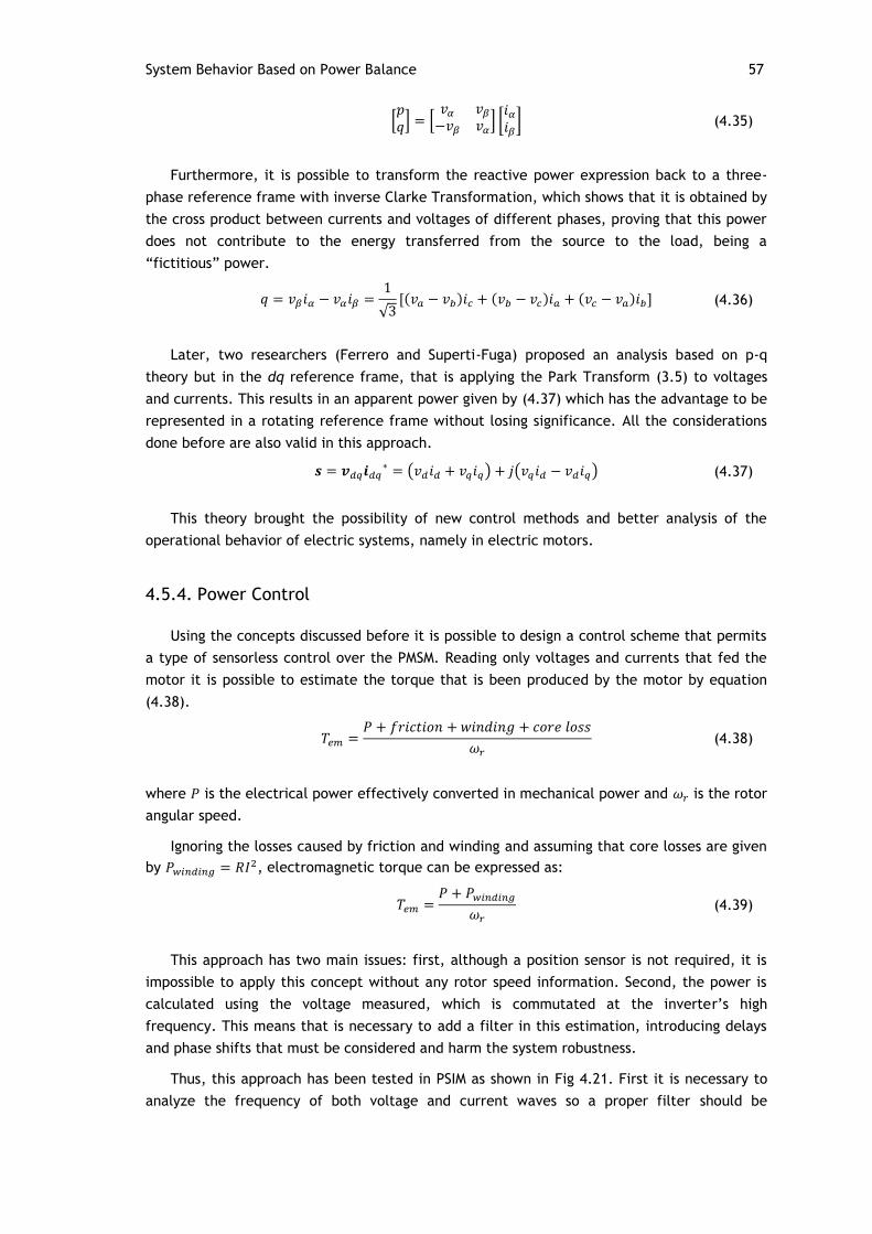
System Behavior Based on Power Balance 57
[ ] [
] [
] (4.35)
Furthermore, it is possible to transform the reactive power expression back to a three-
phase reference frame with inverse Clarke Transformation, which shows that it is obtained by
the cross product between currents and voltages of different phases, proving that this power
does not contribute to the energy transferred from the source to the load, being a
“fictitious” power.
√ [ ] (4.36)
Later, two researchers (Ferrero and Superti-Fuga) proposed an analysis based on p-q
theory but in the dq reference frame, that is applying the Park Transform (3.5) to voltages
and currents. This results in an apparent power given by (4.37) which has the advantage to be
represented in a rotating reference frame without losing significance. All the considerations
done before are also valid in this approach.
( ) ( ) (4.37)
This theory brought the possibility of new control methods and better analysis of the
operational behavior of electric systems, namely in electric motors.
4.5.4. Power Control
Using the concepts discussed before it is possible to design a control scheme that permits
a type of sensorless control over the PMSM. Reading only voltages and currents that fed the
motor it is possible to estimate the torque that is been produced by the motor by equation
(4.38).
(4.38)
where is the electrical power effectively converted in mechanical power and is the rotor
angular speed.
Ignoring the losses caused by friction and winding and assuming that core losses are given
by , electromagnetic torque can be expressed as:
(4.39)
This approach has two main issues: first, although a position sensor is not required, it is
impossible to apply this concept without any rotor speed information. Second, the power is
calculated using the voltage measured, which is commutated at the inverter’s high
frequency. This means that is necessary to add a filter in this estimation, introducing delays
and phase shifts that must be considered and harm the system robustness.
Thus, this approach has been tested in PSIM as shown in Fig 4.21. First it is necessary to
analyze the frequency of both voltage and current waves so a proper filter should be

58 Control of the PMSM
designed. Then a dynamic gain is designed to compensate the signal attenuation caused by
the filter. Active and reactive powers are calculated based on equations from the system
(4.35). Reactive power could later be used for enhancing the control. Finally the torque is
calculated by subtracting the core losses to the power calculated and dividing the result by
the rotor speed. The average value of this result is then calculated.
Fig 4.21 – Sensorless control based on power balance. Top left: Electromagnetic torque calculus; Top right: Dynamic filter gain; Bottom left: Active power calculus; Bottom right: Reactive power calculus.
To better understand the dynamic gain designed it is important to first understand how a
low-pass filter works. The transfer function of a first-order low-pass filter is given by:
⇒
(4.40)
where is the cut-off frequency of the filter.
Control theory says that the gain and phase of (4.40) are given by (4.41) and (4.42),
respectively. The Bode diagram according to equation (4.40), with a cut-off frequency of
5Hz, can also be seen in Fig 4.22. Remember: and .
| | (√ (
)
) (4.41)
(
) (4.42)

System Behavior Based on Power Balance 59
Fig 4.22 - Bode Diagram of a first-order low-pass filter. = 5Hz.
However, to achieve better filtering, a second-order low-pass filter is chosen instead.
This filter has de following transfer function:
⇒
(4.43)
Once again, it is known that the gain and phase of (4.43) are calculated through (4.44)
and (4.45), respectively. The Bode diagram that represents this filter with
is presented in
| | (√(
)
(
)
) (4.44)
(
(
) ) (4.45)

60 Control of the PMSM
Fig 4.23 – Bode Diagram of a second-order low-pass filter. = 5Hz.
This control analysis allow the filter designer to know essentially two things: first, if it is
intended to have the same signal amplitude of the input at the output, as in this case, the
gain of the filter must be amplified by a gain that varies with the frequency of the input
signal, since it introduces attenuation. Second, as it is intended to calculate power and thus
two quantities are needed (voltage and current), both have to be filter (despite the current
signal being already sinusoidal) so their phases are affected by the same phase shift, thus not
interfering in the calculus. With this in mind, the power and consequently the torque are
calculated as shown in Fig 4.21.
Although this technique seems to be very promising, it did not give good results in the
motor control. The author claims that the main reason for that is the startup at zero speed.
Since there is no rotor speed, the torque calculated when the system starts it is theoretically
infinite. More, there are motor losses that are not considered, what could cause inaccuracies
harming the control. Finally, since the motor has a wide speed range and it depends on the
current frequency, the low-pass filter needs to be designed with a very low cut-off
frequency. Although a dynamic gain is designed to compensate the attenuation, at high
frequencies it loses accuracy, again harming the control robustness. Therefore there will not
be presented any simulations results with this technique.
4.6. Summary
The control of the PMSM is presented in this chapter. The strategy, consisting in a torque
reference scheme, is described and 3 different methods are discussed: stator current vector
at 90º, air-gap flux vector at 90º and Maximum Torque Per Ampere. Then, two different
signal generation techniques for the inverter are presented: Sine-PWM and SVM. SVM design is

Summary 61
explained and due to its dynamic characteristics it is considered the best. Three different
controller platforms are then presented: DSP, FPGA and specific application micro-controller.
Their main characteristics are exposed and because of DSP sequential processing
architecture, it is discarded for a possible vehicle application. Among the other two
platforms, FPGA is considered the best because of its processing abilities and parallel
architecture. Four tests were performed, one for each method and another one for MTPA
with SVM. The aim of the last test is to compare sine-PWM with SVM and MTPA method is
chosen because it has the best overall performance. It is proved that SVM has better dynamic
performance than sine-PWM and for that reason is chosen for a future implementation of this
system. Finally the system behavior based on power balance is discussed. P-Q theory is
described in order to allow the system analysis in dq frame. This approach is used as a
position sensorless technique, although without good results. Its implementation is described
but due to the lack of valid results, none are presented.

62 Control of the PMSM

Chapter 5
System Sensorless Control
5.1. Introduction
Controlling a permanent magnet synchronous motor usually requires knowing the rotor
position to perform an effective stator current vector control. This implies the purchase of
sensors which can be expensive. Besides that, considering a vehicle application, more wiring
is needed which decreases the robustness and reliability of the system, increases the need of
maintenance and the inertia of the vehicle and introduces noise problems. Usually this sensor
is a shaft-mounted optical encoder, resolver or Hall sensors. Furthermore, the rotor speed is
also frequently required implying the usage of another sensor.
In order to overcome this problem some new control techniques have emerged based on a
sensorless approach. They consist in estimating the rotor position and speed in order to
accomplish the same results that are obtained if a sensor is used. These techniques can
roughly be divided in the following categories which will be discussed in this chapter:
Back-EMF estimators
State observers
Sliding-mode observers
High-frequency signal injection
PLL-based estimators
5.2. Sensorless Techniques Comparison
This section pretends to briefly describe some sensorless techniques used to control a
PMSM. Although sensorless control is a very recent technique, several solutions are available
in the literature [26]-[40]. Most of them require some kind of startup assistance in order to
achieve proper control of the system. Others are not feasible in vehicles applications. Some
of the techniques described could be put together so better results could be achieved. An
example of this is presented in [26] where Back-EMF estimation is combined with High-
frequency signal injection in a hybrid vehicle application.

64 System Sensorless Control
Back-EMF estimators, State observers and Sliding-mode observers were tested in PSIM
without any good results. However, one of the previous techniques proved to be worthwhile
and it has been implemented with good results: PLL-based position and speed estimator. Its
description and design is detailed on 5.2.5.
5.2.1. Back-EMF Estimator
For this kind of sensorless estimation two stator line voltages and currents measurements
are required. Then, the third line voltage and current is calculated and the Clarke
Transformation is applied to obtain and voltage and current components in the stationary
frame. The stator flux vector module and angle are calculated knowing the and
components of the flux, which are estimated by the expression:
∫ (5.1)
where is the flux, is the voltage, is the stator phase resistor, is the current and
the subscript refers to and components, respectively.
The module and angle of the flux vector is then given by:
| | √
(5.2)
(5.3)
The rotor position is assumed to be given by the angle of stator flux and the speed by its
first derivative. This obviously affects the performance of the controller because the results
critically depend on the accuracy of the estimated flux components which, in turn, depend
on the accuracy of the measured voltages and currents and the integration algorithm chosen.
In addition, this estimation consider that the speed variations are negligible thus ignoring the
rotor flux component for the flux estimation. Although many drift compensations have
been reported, the pure integration in the software or hardware circuits can still be
problematic at low frequencies, where the stator voltage becomes very small and are
dominated by the ohmic voltage drops [27].
5.2.2. State Observer
State observers are other name to closed-loop estimators. That is, estimation of unknown
parameters based on motor’s measurements, with the use of estimation error to adjust the
response of the estimator [28]. State observers are a very common way of applying sensorless
control over PMSM. They usually consist in estimate rotor position by variations in motor’s
parameters, as inductance variations due to magnetic saturation, which are noticed through
mathematical calculations knowing motor’s model equations. The INFORM technique
(“INdirect Flux detection by On-line Reactance Measurement”) was proposed by Schroedl [29]
and is based on real-time inductance measurements using saliency and saturation effects.
During a short time interval, the “complex INFORM reactance” is calculated for estimating
Sensorless Techniques Comparison 65
flux angle. However, this technique must be combined with observer techniques to work
properly in whole speed range [30].
Other observers known for PMSM sensorless control are Extended Luenberger Observer
(ELO) and Extended Kalman Filter (EKF). ELO is applicable to non-linear, time-variant and
deterministic systems. EKF is a recursive optimum-state estimator, able to provide optimum
filtering of the noises in measurements if the covariances of these noises are known. It is an
optimal stochastic observer what makes it a viable candidate for the on-line determination of
the rotor position and speed of PMSM. “However, none of the practical industry applications
of EKF-based sensorless PMSM control has been reported due to the technical difficulties,
which may include: 1) detailed dynamic model of PMSM with initial rotor position; 2)
formulation of the EKF model in closed form; 3) discrete-time model of the overall controlled
system and details of power electronics circuitry and implementation; 4) complex methods
for correcting the rotor flux variations; 5) initial speed position convergence; 6)
computational expense, specific design, tuning criteria and so on” [27].
5.2.3. Sliding-mode Observer
Among the existing sensorless approaches, sliding mode observer has been recognized as
one of the best techniques due to its advantages in robustness to disturbances and low
sensitivity to parameter variations.
Briefly, sliding mode observer techniques are based on the state variables of the PMSM. A
sliding surface is defined as well as two limits for that surface, creating a hysteresis window.
The controlled variable is intended to track that surface and slide along it within the limits
imposed.
Some variations of sliding-mode observers are presented in literature [31]-[34].Yoon-Seok
Han presented a technique that uses Lyapunov functions for determining the adaptive law for
the speed and stator resistance estimator. This technique showed good results with respect
to variations in stator resistance [31]. Elbuluk investigated a sliding mode observer for
estimating the rotor position and speed of PMSM considering motor’s parameters variations.
Instead of directly using filtered switching signals by a low-pass filter, an observer is designed
to undertake the filtering task for the estimated back-EMF. It is stated that the observer has
the structure of an extended Kalman filter and is expected to have high filtering properties.
However, no experimental results are presented [33]. In other article ([34]) Elbuluk claims
that the sliding mode technique applied is robust to motor’s parameters variations. The
results show a parameter detuning of 200% with good results.
5.2.4. High-frequency Signal Injection
High-frequency injection sensorless techniques basically consist in injecting a high-
frequency voltage signal in any phase of the motor assuming that is the direction of the rotor
flux vector (or d-axis) and measure the current. The current will be highest when the
inductance is lowest, that is through the axis. Similarly, the measured current will be
lowest when the inductance is higher, meaning that’s the direction of axis. Of course that
this is only valid in motors where , otherwise this technique must not be considered

66 System Sensorless Control
valid. Once motors’ parameters are known, the measurement of these currents and and
extraction can align the supposed reference frame with the real rotor position and therefore
a sensorless system is achieved.
However, these techniques require high precision and fast measurement, and fast signal
processing capability, which inevitably will increase the complexity and cost of control
system. Furthermore, the injected high frequency voltages may also cause more torque
ripple, shaft vibration and audible noises. Due to the constraints of the maximum PWM
switching frequency and the geometry of rotor, such techniques usually work to some specific
motors in the limited operating speed range, i.e., only at standstill and low speeds [27].
5.2.5. PLL-based Estimator
This technique, based on [8], pretends to estimate rotor position and speed by
synchronizing the estimated reference frame with the real rotor reference frame, which has
the rotor flux vector aligned with the d-axis. This is achieved estimating the back-EMF vector
created by the rotor’s PMs and bringing its d- component in the estimated reference frame to
zero. That assumption means that the rotor’s back-EMF vector is aligned with the actual q-
axis, and consequently the rotor flux vector is aligned with d-axis, as it is supposed to be. Fig
5.1 represents this logic in the vector form. The circumflex accent means that the unit
referred is estimated and the angle between the reference frames is defined by .
Fig 5.1 – PLL-based estimator logic [8].
From Fig 5.1 it is possible to establish the following geometrical relationship:
(5.4)
(5.5)
To estimate the d- and q- components of back-EMF in the estimated reference frame,
motor’s equations are used:

Sensorless Techniques Comparison 67
(5.6)
(5.7)
The estimator logic is described as following: is compared with a reference (that is
zero) and the error enters in a PI controller. The output of the PI is the estimated speed
which is then integrated in order to obtain the estimated position. The position is used to
correctly apply the Park Transform to the three-phase voltages and currents that are being
measured from the motor. Their d- and q- components, and the estimated angular speed, are
then used to calculate the back-EMF dq components as described before. So, when ,
means that the error is zero and that the position estimated is actually the real one. This
means that the speed from which the position is calculated is also accurate, indicating that
the two frames are overlapped.
This technique of estimating the rotor’s position can be used since standstill without any
other auxiliary system for starting the motor. However, until enough speed to generate
measurable back-EMFs is developed, the estimation has some imprecisions. This could be a
problem or not, depending on the transmission rate used in the vehicle. If the motor could
reach about 80 rad/s in less than a second, the driver does not even notice the oscillations
that occur in the first milliseconds. These results are analyzed later in this chapter.
5.2.5.1. PLL Controller Design
According to [8], since the calculation of the back-EMFs should be the fastest element in
the sensorless control scheme, it can be approximated by its gain:
| | √
(5.8)
As shown in (5.8), the d- component of the back-EMF has a negative signal with respect
to the rotor position , so the PI controller must have negative gain to compensate for this.
By replacing (5.4) and (5.5) into (5.8) the gain of the estimator becomes proportional to the
rotor speed according to the following relation:
(5.9)
By inserting a linearization gain before the PI, as shown in (5.11) it is possible to cancel
the speed-dependent gain nature of the PLL and to tune the PI with positive gains. The gains
of the PI, and , can be obtained after the transfer function of the PLL linearized is
known. According to [8] they can be calculated by:
{
(5.10)
where is the desired damping factor and is the desired bandwidth of the rotor position
controller.
The linearization gain is then given by:

68 System Sensorless Control
√
(5.11)
This approximation is valid assuming that is controlled to zero and reaches that value
in a short amount of time. Considering this brings a big computational advantage of not
having a square root. From the controller platform point of view, this could represent the
saving of several micro-seconds, which could be critical.
Good results with this technique are achieved with Matlab Simulink working with PSIM via
SimCoupler. This interface lets both simulation platforms run simultaneously allowing, for
example, the implementation of the power system in PSIM and all the control in Simulink.
Because PSIM is much better in dealing with power systems, and Simulink has many
advantages over PSIM in terms of user interface simplicity, pre-built optimized function
blocks and some toolboxes created specifically for some controller platforms (like DSP or
FPGA), having the possibility of join this two virtual environments in one single system
(simulation) is pretty useful.
The PLL-based sensorless logic described before is implemented in Simulink using
SimCoupler to interact with PSIM where the power stage is, and the control over the motor is
accomplished. The usage of Simulink to implement the control could be an advantage later
when the program needed to be programmed in FPGA, because of the toolboxes that Xilinx
provide for Matlab. Also, Simulink provides various types of resolving the differential
equations that represent the model, whereas PSIM only allows the change in integration fixed
time-step parameter, using the trapezoidal rule integration method. Simulink provides many
solver types, either for Fixed Time-step as for Variable Time-step. Although each solver apply
a different numerical method to solve the ODEs (Ordinary Differential Equation) of the
system, many of them are variants of Runge-Kutta method. So, as at first sight it is not
necessary a method that is more accurate, the solver chosen for this application is “ode4
Fourth-Order Runge-Kutta” with a Fixed-Step time of 0.1μs. More information about the
Simulink solver is available in [41].
5.3. Sensorless Control Results
The results obtained with sensorless control are pretty satisfactory. Although they are not
as good as with the use of a speed sensor (as expected), the control actually behaves as it
should and the motor operation can be assured according to what has been said before in
section 4.2.
The PI gains were adjusted as the PI’s of torque and in the previous control. As the
input of the PLL PI is the error of a back-EMF and the output is supposed to be an angular
speed, according to (5.4) the proportional gain should be around the inverse of the value of
rotor’s permanent magnets flux, times the number of pole pairs. The integral gain should be
at least 10 times bigger, so the practical experience says. Thus, these gains were adjusted by
analysis of the system behavior among various tests. The gains used are described in Table
5.1 and the PLL-based sensorless speed and position estimator implemented in Simulink is
shown in Fig 5.2.

Sensorless Control Results 69
Table 5.1 – Sensorless PLL PI gains.
60
1500
Fig 5.2 - PLL-based sensorless speed and position estimator implemented in Simulink.
In Fig 5.2 it is possible to see the PLL-based logic in the upper left corner, with the error
measurement, the linearization gain, the PI controller which generates the rotor electrical
angular speed and its integration to generate rotor position. This position is then used to
generate dq components to be used in and estimation, represented by the two blocks
on the bottom. The speed and position estimated, as well as dq voltage and current
components, are sent to PSIM through SimCoupler block on the right of the Fig 5.2, which also
receives three-phase measured voltages and currents to be converted.
To demonstrate the correct operation of the motor with the control method described
and with sensorless PLL-based technique, a complete test is designed. The motor starts with
an increasing torque reference and without load so the speed can increase. Then, it is
introduced a constant torque load to the motor with a torque equal to reference torque so
the speed can become constant. Then, the load torque increases again to simulate the
initiation of road ascension or an obstacle on the road, and consequently the speed
decreases. The torque reference rises to compensate this and the speed rises again. The
torque is then set to zero, to simulate a complete pedal lifting, and it is possible to see the
speed decreasing to zero.
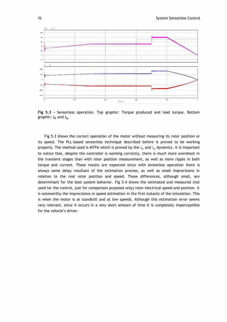
70 System Sensorless Control
Fig 5.3 - Sensorless operation. Top graphic: Torque produced and load torque. Bottom
graphic: and .
Fig 5.3 shows the correct operation of the motor without measuring its rotor position or
its speed. The PLL-based sensorless technique described before is proved to be working
properly. The method used is MTPA which is proved by the and dynamics. It is important
to notice that, despite the controller is working correctly, there is much more overshoot in
the transient stages than with rotor position measurement, as well as more ripple in both
torque and current. These results are expected since with sensorless operation there is
always some delay resultant of the estimation process, as well as small imprecisions in
relation to the real rotor position and speed. These differences, although small, are
determinant for the best system behavior. Fig 5.4 shows the estimated and measured (not
used for the control, just for comparison purposes only) rotor electrical speed and position. It
is noteworthy the imprecisions in speed estimation in the first instants of the simulation. This
is when the motor is at standstill and at low speeds. Although this estimation error seems
very relevant, since it occurs in a very short amount of time it is completely imperceptible
for the vehicle’s driver.

Sensorless Control Results 71
Fig 5.4 – Sensorless operation. Top graphic: Rotor electrical angular speed (Wr – estimated; Wr_real – measured); Bottom graphic: Rotor electrical position (theta – estimated; theta_real – measured).
5.4. Summary
Several sensorless techniques for controlling the PMSM are presented. They are divided in
five categories: back-EMF estimators, state observers, sliding-mode observers, high-frequency
signal injection techniques and PLL-based estimators. Each of these categories is described
and discussed. Due to the results obtained in PSIM, only PLL-based estimator is further
analyzed in this document. Its implementation is explained and the results obtained with Co-
Simulation between PSIM and Simulink are discussed. The system proved to be controllable
with positive torque reference without any position or speed sensor, validating the estimator
operability in this range.

72 System Sensorless Control

Chapter 6
System Validation
6.1. Introduction
In this Chapter a validation of the system is done. Having in considerations what has been
said so far, a detailed analysis about regenerative braking and dynamic performance of the
sensorless traction control system is done. Also, several considerations about a future
implementation of the work here described are drawn. Finally, some suggestions about what
could possibly be done to enhance this work are given.
6.2. Regenerative Braking
A simulation of a real road situation is done in Chapter 4 which included a braking
intervention, with negative torque reference. However, that system is using a speed sensor,
from which the position information is taken. In Chapter 5 a validation of sensorless system
control is done, again trying to simulate a real road situation, but this time without applying
a braking torque. That test is performed here and the results are analyzed.
Before the description and analysis of the simulation results, an important remark must
be done. As said in section 5.2.5.1 the solvers available for simulation in Simulink are variants
of Runge-Kutta method. As it turns out, this mathematical method is not sufficient to
perform an accurate simulation with the requirements of this system. Although the system
works fine when positive torque reference is given, with sensorless operation in Simulink and
all the power and control stages in PSIM, for negative torque reference that does not happen.
The author considers that the conditions imposed by the system when calculating the dq
components of the back-EMFs at low and negative torque (which means that is also very
small or negative) introduce discontinues or undefined solutions, that Runge-Kutta method
cannot deal with. As the author in [42] states: “Runge-Kutta is a mathematical integration
method based on Euler's method, which is not recommended for practical use for mainly 2
reasons: the method is not very accurate when compared to other, fancier, methods run at
the equivalent step size, and neither is it very stable”. Moreover, when talking about other
methods for resolving ODEs, as Bulirch-Stoer or predictor-corrector methods, the author

74 System Validation
creates an analogy saying that “Those methods are the high-strung racehorses. Runge-Kutta is
for ploughing the fields”. For these reasons, the exactly same PLL-based estimator designed
in Simulink is transposed to PSIM. This system, with the speed and position estimator
designed in PSIM as shown in Fig 6.1, is analyzed in this chapter.
Fig 6.1 – PLL-based speed and position estimator implemented in PSIM.
The C-Blocks presented are used to calculate the average value of their input by using a
sliding-window technique. It consists in saving the last X values of the input (being X the
amount of samples defined by user) and dividing that sampled values by X. The output is
updated each X samples, maintaining its value until another cycle is completed.
The situation that has been tested is described as follows: the motor starts from standstill
without load torque and achieves the reference of 70Nm with the speed rising accordingly. At
0.3s the torque decreases to 50Nm and a load is introduced at 0.4s with a constant torque of
50Nm (same as the reference given). The speed is expected to become constant. The same
load is maintained until 0.6s. At 0.5s a braking torque is applied, of -50Nm. It remains there
until second 0.7, where “the braking pedal” is released slowly. The motor keeps running
because of the inertia since no other force is applied to it from the moment that “braking
pedal” is released. The torque and current results can be seen in Fig 6.2. As expected there
is a small error between calculated and effective electromagnetic torque because of the
error in speed estimation.

Regenerative Braking 75
Fig 6.2 - Sensorless operation with regenerative braking. Top graphic: Torque calculated
( ) and torque produced ( ). Bottom graphic: and .
As for the speed and position estimation, the results are presented in Fig 6.3. As shown,
there is the same speed estimation error at low speeds that is present with the sensorless
algorithm designed in Simulink. But despite that, the result does not affect the stability of
the system, neither the position estimation. There are also some estimation imperfections
every time the speed has an accentuated change. That would not occur in a physical
application like an electric bus because the inertia is such that does not allow quick speed
changes thus preventing this singularity from happening. It is also remarkable the result
obtained for the position estimation. In the maxim error registered is of 0.4% at 6.014s. The
detailed error is presented in Fig 6.4.
Fig 6.3 - Sensorless operation. Top graphic: Rotor electrical angular speed (Wr – estimated; Wr_real – measured); Bottom graphic: Rotor electrical position (theta – estimated; theta_real – measured).

76 System Validation
Fig 6.4 – Detail of the estimated position error.
It is important to make sure that the current is actually flowing from the motor to the DC-
bus when the motor is braking. To do that a current probe is used in DC-bus. As the current
on DC-bus is not filtered and only its average value is important to analyze at this time, a C-
Block to calculate its average value is used as described before for the speed and back-EMF
components. The result is shown in Fig 6.5.
Fig 6.5 - DC-bus average current in traction and braking, with sensorless operation.
It is important to notice two things in this figure. The first is that the DC-bus current
inverts direction according to the torque produced. That means that the current is flowing
from the motor to the DC-bus when a negative torque is applied, thus effectively achieving
energy regeneration while braking. Another important aspect is the fact that the current is
null when no torque and no load is applied to the motor. In the situation simulated only the
inertia is considered from 0.9s to the end. In this case, the motor maintains the speed but no
regeneration is performed because the torque reference is zero. This also can be seen as if
the inverter is an open circuit, thus the current flowing is zero. As the rotor is spinning, a
back-EMF is induced at the terminals of the motor, which is wasted since there’s no current
flowing.
To achieve a better performance and to extend at the maximum the battery range, the
energy generated when the vehicle is running and there is no braking nor acceleration torque
must be harnessed. Conceptually this is done giving a negative torque reference when none
of the vehicle’s pedals are pressed and the speed is rising, indicating that the vehicle is going
down. Mathematically this behavior can be understood by electromagnetic torque mechanical
equation presented in (4.1) and repeated here for convenience.
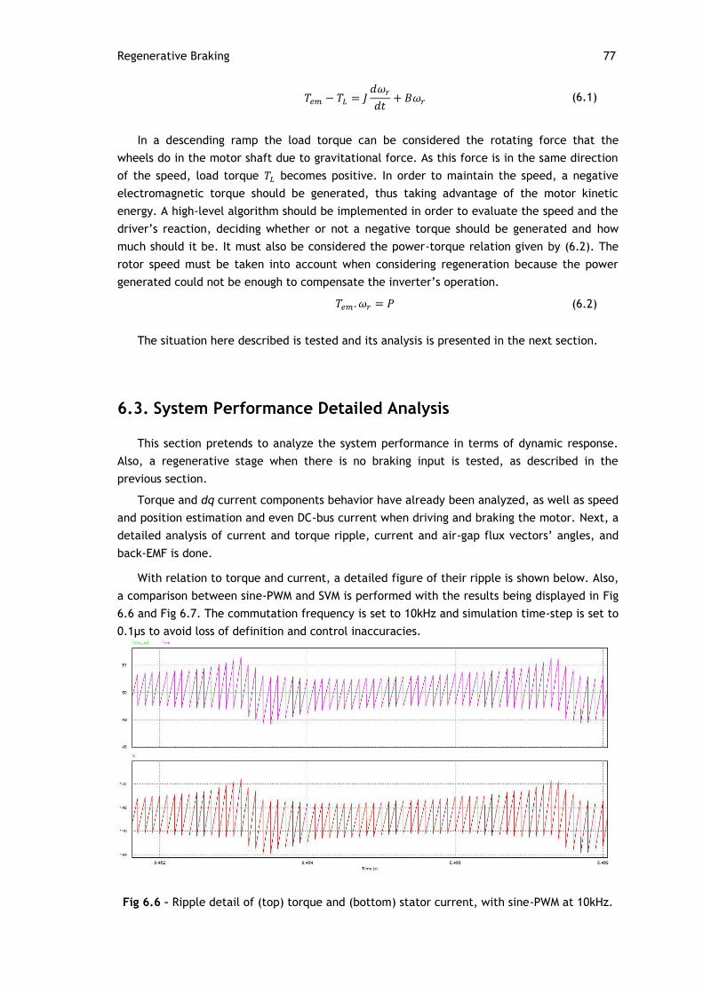
Regenerative Braking 77
(6.1)
In a descending ramp the load torque can be considered the rotating force that the
wheels do in the motor shaft due to gravitational force. As this force is in the same direction
of the speed, load torque becomes positive. In order to maintain the speed, a negative
electromagnetic torque should be generated, thus taking advantage of the motor kinetic
energy. A high-level algorithm should be implemented in order to evaluate the speed and the
driver’s reaction, deciding whether or not a negative torque should be generated and how
much should it be. It must also be considered the power-torque relation given by (6.2). The
rotor speed must be taken into account when considering regeneration because the power
generated could not be enough to compensate the inverter’s operation.
(6.2)
The situation here described is tested and its analysis is presented in the next section.
6.3. System Performance Detailed Analysis
This section pretends to analyze the system performance in terms of dynamic response.
Also, a regenerative stage when there is no braking input is tested, as described in the
previous section.
Torque and dq current components behavior have already been analyzed, as well as speed
and position estimation and even DC-bus current when driving and braking the motor. Next, a
detailed analysis of current and torque ripple, current and air-gap flux vectors’ angles, and
back-EMF is done.
With relation to torque and current, a detailed figure of their ripple is shown below. Also,
a comparison between sine-PWM and SVM is performed with the results being displayed in Fig
6.6 and Fig 6.7. The commutation frequency is set to 10kHz and simulation time-step is set to
0.1μs to avoid loss of definition and control inaccuracies.
Fig 6.6 – Ripple detail of (top) torque and (bottom) stator current, with sine-PWM at 10kHz.

78 System Validation
As shown in Fig 6.6, the maximum torque ripple with sine-PWM at 10kHz is about 2,5Nm
and the average is about 1Nm, which is not much ( considering the torque effectively
produced of 50Nm. With respect to stator current, the maximum existent ripple is of about
6A and the average ripple is about 2,5A. Once again, relatively to the effective current, the
ripple is no considerable ( , although the ideal goal is ripple.
As for SVM, the results presented in Fig 6.7 show almost the same results: a torque ripple
of about 2Nm and a stator current ripple of about 6A in the worst case and about 2,5A in the
better case, making an average of about 4A of ripple.
Fig 6.7 - Ripple detail of (top) torque and (bottom) stator current, with SVM at 10kHz.
An unexpected conclusion can be drawn from these results: the SVM has the same results
as the sine-PWM with respect to torque and current ripple when the system is working
sensorless. It is settled before that the inverter’s signal generation would be done with SVM
because the results obtained justified the choice. However, in this case, that does not
happen. The reason for that may be the fact that in sensorless operation it is needed a lot
more processing abilities that may interfere with the SVM routine. Since SVM require much
more computation than sine-PWM to be performed correctly, and since the speed and
position estimation also introduce delays and errors in the system, those may be the reasons
why these two techniques almost do not distinguish themselves with respect to ripple
generation. However, using a controller that has high processing performance, like the FPGA,
the results could be different, and SVM should have better results than sine-PWM. Moreover,
SVM has a better DC usage (about 15% more than sine-PWM) that could be useful in a vehicle
application like this one because it can deliver more power to the motor with the same
battery capacity. This leads to the usage of less current which decreases the inverter losses,
increasing system’s efficiency.
With relation to the angles of the current and air-gap flux vectors, they can be seen in Fig
6.8. It is possible to see the variations in both of them as the torque requirements change, as
well as the changes in the angle between them. Remember: that angle, , is the torque

System Performance Detailed Analysis 79
angle. It can be observed in more detail in Fig 6.9 for positive torque and in Fig 6.10 for
negative torque.
Fig 6.8 – Stator current vector angle and air-gap flux vector angle .
The final blur presented in the figure is because the angles are calculated using the
arctangent function. When dq components are zero, the result becomes undefined and
simulation result is that of the last instants of Fig 6.8.
It is important to notice that torque angle changes with torque necessities. Although the
control method does not control this angle directly, it is inevitable that it changes according
to torque requests. However, since the control method used is MTPA, as explained before it
tries to use the less current possible to a given torque reference. So, as both current and air-
gap flux vectors depend on dq current components, the changes in their amplitudes are
directly proportional to each other and consequently the torque angle does not react exactly
as expected, that is becoming bigger when more torque is needed. In fact, the torque
produced is maximum when torque angle is 90º. However, it does not mean that that’s the
situation in which less current is used for a given torque. As shown, the torque angle is less
when torque reference is 70Nm than when it is 50Nm, but the current is the minimum in any
case, and that’s what that matters in a vehicle application. Fig 6.9 and Fig 6.10 show the
detail of the torque angle for positive and negative torque, respectively.
Fig 6.9 – Torque angle detail for positive torque.
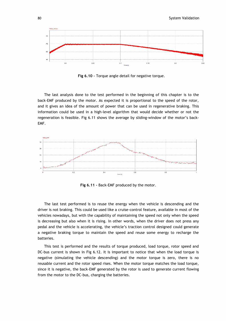
80 System Validation
Fig 6.10 – Torque angle detail for negative torque.
The last analysis done to the test performed in the beginning of this chapter is to the
back-EMF produced by the motor. As expected it is proportional to the speed of the rotor,
and it gives an idea of the amount of power that can be used in regenerative braking. This
information could be used in a high-level algorithm that would decide whether or not the
regeneration is feasible. Fig 6.11 shows the average by sliding-window of the motor’s back-
EMF.
Fig 6.11 – Back-EMF produced by the motor.
The last test performed is to reuse the energy when the vehicle is descending and the
driver is not braking. This could be used like a cruise-control feature, available in most of the
vehicles nowadays, but with the capability of maintaining the speed not only when the speed
is decreasing but also when it is rising. In other words, when the driver does not press any
pedal and the vehicle is accelerating, the vehicle’s traction control designed could generate
a negative braking torque to maintain the speed and reuse some energy to recharge the
batteries.
This test is performed and the results of torque produced, load torque, rotor speed and
DC-bus current is shown in Fig 6.12. It is important to notice that when the load torque is
negative (simulating the vehicle descending) and the motor torque is zero, there is no
reusable current and the rotor speed rises. When the motor torque matches the load torque,
since it is negative, the back-EMF generated by the rotor is used to generate current flowing
from the motor to the DC-bus, charging the batteries.
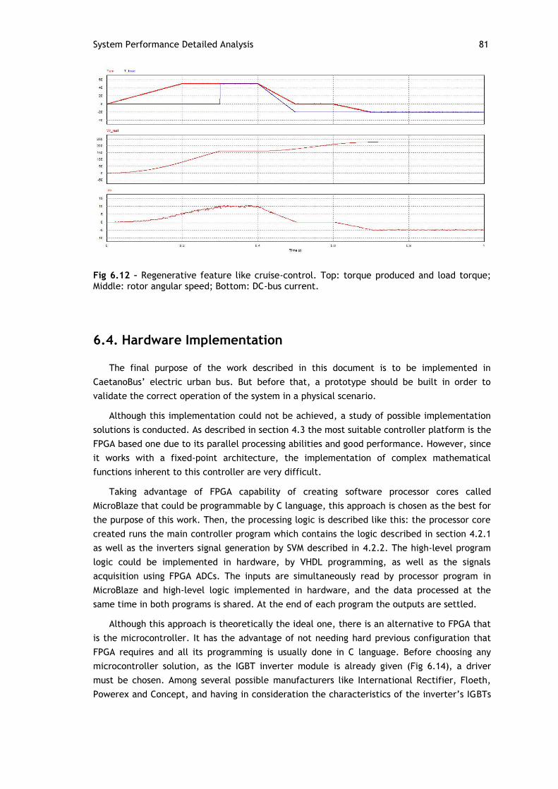
System Performance Detailed Analysis 81
Fig 6.12 – Regenerative feature like cruise-control. Top: torque produced and load torque; Middle: rotor angular speed; Bottom: DC-bus current.
6.4. Hardware Implementation
The final purpose of the work described in this document is to be implemented in
CaetanoBus’ electric urban bus. But before that, a prototype should be built in order to
validate the correct operation of the system in a physical scenario.
Although this implementation could not be achieved, a study of possible implementation
solutions is conducted. As described in section 4.3 the most suitable controller platform is the
FPGA based one due to its parallel processing abilities and good performance. However, since
it works with a fixed-point architecture, the implementation of complex mathematical
functions inherent to this controller are very difficult.
Taking advantage of FPGA capability of creating software processor cores called
MicroBlaze that could be programmable by C language, this approach is chosen as the best for
the purpose of this work. Then, the processing logic is described like this: the processor core
created runs the main controller program which contains the logic described in section 4.2.1
as well as the inverters signal generation by SVM described in 4.2.2. The high-level program
logic could be implemented in hardware, by VHDL programming, as well as the signals
acquisition using FPGA ADCs. The inputs are simultaneously read by processor program in
MicroBlaze and high-level logic implemented in hardware, and the data processed at the
same time in both programs is shared. At the end of each program the outputs are settled.
Although this approach is theoretically the ideal one, there is an alternative to FPGA that
is the microcontroller. It has the advantage of not needing hard previous configuration that
FPGA requires and all its programming is usually done in C language. Before choosing any
microcontroller solution, as the IGBT inverter module is already given (Fig 6.14), a driver
must be chosen. Among several possible manufacturers like International Rectifier, Floeth,
Powerex and Concept, and having in consideration the characteristics of the inverter’s IGBTs
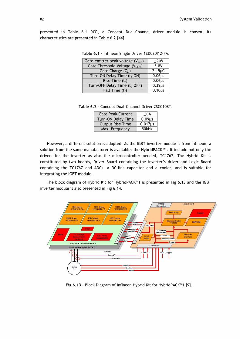
82 System Validation
presented in Table 6.1 [43], a Concept Dual-Channel driver module is chosen. Its
characteristics are presented in Table 6.2 [44].
Table 6.1 – Infineon Single Driver 1ED020I12-FA.
Gate-emitter peak voltage (VGES) V
Gate Threshold Voltage (VGEth) 5.8V
Gate Charge (QG) 2.15μC
Turn-ON Delay Time (td ON) 0.06μs
Rise Time (tr) 0.06μs
Turn-OFF Delay Time (td OFF) 0.39μs
Fall Time (tf) 0.10μs
Table 6.2 - Concept Dual-Channel Driver 2SC0108T.
Gate Peak Current A
Turn-ON Delay Time 0.09μs
Output Rise Time 0.017μs
Max. Frequency 50kHz
However, a different solution is adopted. As the IGBT inverter module is from Infineon, a
solution from the same manufacturer is available: the HybridPACK™1. It include not only the
drivers for the inverter as also the microcontroller needed, TC1767. The Hybrid Kit is
constituted by two boards, Driver Board containing the inverter’s driver and Logic Board
containing the TC1767 and ADCs, a DC-link capacitor and a cooler, and is suitable for
integrating the IGBT module.
The block diagram of Hybrid Kit for HybridPACK™1 is presented in Fig 6.13 and the IGBT
inverter module is also presented in Fig 6.14.
Fig 6.13 – Block Diagram of Infineon Hybrid Kit for HybridPACK™1 [9].

Hardware Implementation 83
Fig 6.14 – Infineon IGBT driver module for HybridPACK™1.
6.5. Summary
As the control strategy and methods have already been discussed and their results
presented, as well as with sensorless control with positive torque reference, the last test
remaining is the validation of regenerative braking without speed or position sensors. This
test was only possible with the implementation of sensorless technique in PSIM. That is
because of the integration method of Simulink - Runge-Kutta – which is not capable of dealing
with some singularities existent when a negative reference torque is given. The simulation
results are presented and discussed, proving the successful operability of the system in
several load conditions. A detailed analysis of torque, current and flux is also performed.
Lastly, a possible solution for controller platform, inverter and drivers to physical
implementation of the system is presented.

84 System Validation
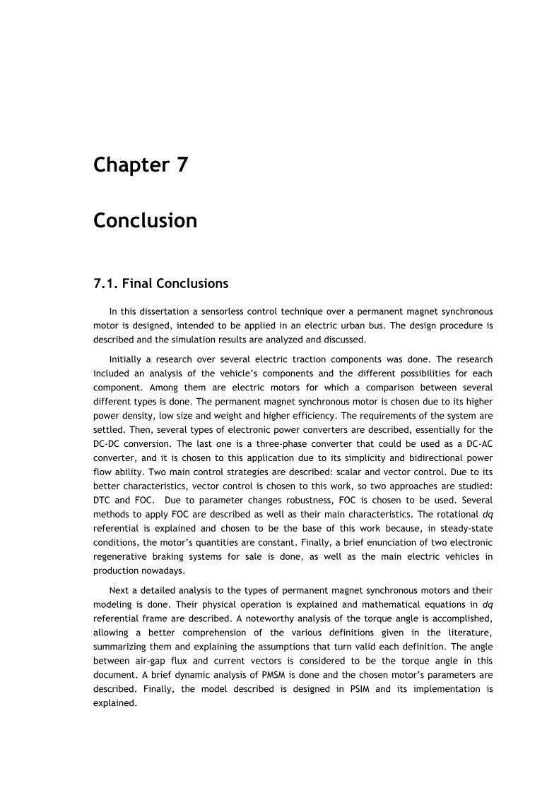
Chapter 7
Conclusion
7.1. Final Conclusions
In this dissertation a sensorless control technique over a permanent magnet synchronous
motor is designed, intended to be applied in an electric urban bus. The design procedure is
described and the simulation results are analyzed and discussed.
Initially a research over several electric traction components was done. The research
included an analysis of the vehicle’s components and the different possibilities for each
component. Among them are electric motors for which a comparison between several
different types is done. The permanent magnet synchronous motor is chosen due to its higher
power density, low size and weight and higher efficiency. The requirements of the system are
settled. Then, several types of electronic power converters are described, essentially for the
DC-DC conversion. The last one is a three-phase converter that could be used as a DC-AC
converter, and it is chosen to this application due to its simplicity and bidirectional power
flow ability. Two main control strategies are described: scalar and vector control. Due to its
better characteristics, vector control is chosen to this work, so two approaches are studied:
DTC and FOC. Due to parameter changes robustness, FOC is chosen to be used. Several
methods to apply FOC are described as well as their main characteristics. The rotational dq
referential is explained and chosen to be the base of this work because, in steady-state
conditions, the motor’s quantities are constant. Finally, a brief enunciation of two electronic
regenerative braking systems for sale is done, as well as the main electric vehicles in
production nowadays.
Next a detailed analysis to the types of permanent magnet synchronous motors and their
modeling is done. Their physical operation is explained and mathematical equations in dq
referential frame are described. A noteworthy analysis of the torque angle is accomplished,
allowing a better comprehension of the various definitions given in the literature,
summarizing them and explaining the assumptions that turn valid each definition. The angle
between air-gap flux and current vectors is considered to be the torque angle in this
document. A brief dynamic analysis of PMSM is done and the chosen motor’s parameters are
described. Finally, the model described is designed in PSIM and its implementation is
explained.

86 Conclusion
The core of this dissertation is the control design described in Chapter 4. First it is
described the strategy of control that is based on a torque reference. Then, three different
methods are explained and implemented in PSIM so they could be tested. Two control signal
generation techniques for the inverter are described: sine-wave PWM and Space Vector
Modulation. Due to its better dynamic and steady-state results, SVM is chosen as the best
technique. Then, the basic operation of proportional-integral controllers chosen is detailed
and their tuning is explained. Two PIs are used for this work, one that regulates the current
and other for the torque (which is proportional to current). Three possible controller
platforms are described: DSP, FPGA and micro-controller. It is decided that, in a possible
future implementation, FPGA is the best having in consideration the requirements of the
system. Also, a specific micro-controller for vehicles application could be a good choice. The
results obtained with the three methods are showed and analyzed and because of the better
results obtained from MTPA, it is chosen to compare sine-PWM and SVM control signal
generation. It is concluded that SVM has better results and for that reason it is chosen to be
used in this work. Lastly, the system behavior based on power balance is done with the
intention of implementing a possible sensorless solution. Regardless of the good theoretical
results, the simulation tests are not conclusive and for that reason this approach is discarded.
The power balance sensorless approach led the way to other techniques of controlling the
motor without the need of measuring its speed and position. So, a study of several different
strategies used nowadays is done and among the options available in the literature, the one
that seemed perfect for the purpose of this work is the PPL-based speed and position
estimator. For that reason it is chosen to be implemented. The detailed analysis of this
technique is done and the results of its implementation in Simulink (working simultaneously
with PSIM by SimCoupler Module) are tested. The results for several positive torque
references are analyzed. It is concluded that this approach allow the control of the PMSM and
with good dynamic responses.
Finally a system validation is done with detailed analysis of current and torque
waveforms, as well as back-EMF generated, current and air-gap flux vectors’ angles, and DC-
current to prove the ability of regenerative braking. The possibility of regenerating energy in
a descending road even without braking is tested successfully. This approach allows an even
better range extender for the batteries. In the end, the pretended hardware implementation
is described, explaining the principle of operation of FPGA as well as the inverter and drives
chosen.
Although this work does not include a physical implementation to validate in laboratory
the results obtained, the tests performed in simulation environment were exhaustive,
covering several possible real situations (but with time intervals much shorter than the real
ones, which guarantee the correct operation of the system in slower tests) and allow the
conclusion that it is possible to implement the control designed in a real motor with good
results. Furthermore, it is possible to conclude that the method used, MTPA, is the most
appropriate for a vehicle application since the current used for the same torque is minimum,
giving the higher battery range comparatively to other control strategies. Also, the results
obtained with sensorless operation allow the conclusion that it is the better approach to the
PMSM control since it has the same overall performance that a system with speed and position
sensors, with the advantage of need less wiring and electrical equipment.

Final Conclusions 87
The development of this work allowed consolidating the knowledge acquired during the
course, with emphasis in power electronics, movement control, signal processing and
controllers design. It also improved some soft-skills like the ability of project management,
self-discipline, advanced skills in simulation software and writing in foreign language.
7.2. Future Work
In this section several suggestions of possible expansions to the work here described are
presented.
Accomplish a practical implementation of this control in a real PMSM. As already
described, the best solution would be with a FPGA controller platform.
Implement the high-level algorithm to deal with regenerative and emergency
braking. In this case, the algorithm should apply the mechanical brake rather than
the electrical brake, wasting the kinetic energy but stopping the vehicle safely.
Apply power balance approach here described to control the motor without rotor
position sensor. Several signal filtering techniques should be tested to achieve the
best results.
Have in consideration the permanent magnets’ magnetic saturation limits to
perform a more realistic simulation and to stipulate more accurately the limits of
the controller and possible dynamic adaptation.
Try different controllers other than PI in order to achieve better dynamic
response. A possible alternative would be an artificial neural-network that could
auto-adapt to driver’s behavior.

88 Conclusion

References
[1] C.C. Chan, “The State of the Art of Electric and Hybrid Vehicles”, Proc. IEEE, Vol. 90, No.
2, February 2002.
[2] Comparing motor-control techniques. Available in
http://www.ecnmag.com/Articles/2009/10/Comparing-motor-control-techniques/.
Access in January 12, 2012.
[3] A. Kawamura et al. “State-of-the-Art High Power Density and High Efficiency DC-DC
Chopper Circuits for HEV and FCEV Applications”, 13th Int. Power Electronics and Motion
Control Conference, 2008.
[4] Huafeng Xiao and Shaojun Xie, Member, IEEE, “A ZVS Bidirectional DC–DC Converter With
Phase-Shift Plus PWM Control Scheme”, IEEE Trans. Power Electron. Vol. 23, No. 2, March
2008.
[5] Lung-Sheng Yang and Tsorng-Juu Liang, Senior Member, IEEE, “Analysis and
Implementation of a Novel Bidirectional DC–DC Converter”, IEEE Trans. Ind. Electron.,
Vol. 59, No. 1, January 2012.
[6] Bogdan M. Wilamowski and J. David Irwin, The Industrial Electronics Handbook - Power
Electronics and Motor Drives, 2nd Edition. Taylor and Francis Group, LLC 2011.
[7] Jun Kang, Ph.D. “Control Engeneering – Yaskawa”. Available in
http://www.yaskawa.com/site/dmdrive.nsf/link2/NKOE-
84VL6B/$file/PR.ControlEngineering.05.pdf. Access in May 23, 2012.
[8] Rolando P. Burgos et al. “Design and Evaluation of a PLL-Based Position Controller for
Sensorless Vector Control of Permanent-Magnet Synchronous Machines”, 2006 © IEEE.
[9] Infineon Technologies AG, "Hybrid Kit for HybridPACK™1: Evaluation Kit for Applications
with HybridPACK™1 Module," vol. V2.5, 2012-03-30, 2012.
[10] Ricardo Soares, “Traction Control for Hybrid Electric Vehicles”, to be published in July
2012.
[11] F. P. Lopes, “Estudo e Comparação de Diferentes Métodos de Controlo de Motores
Síncronos com Ímanes Permanentes,” M.S. thesis, Dept. Electro. Eng., FEUP, Porto,
Portugal, 2008.
[12] Howard C. Lovatt et al. “Design Procedure for Low Cost, Low Mass, Direct Drive, In-Wheel
Motor Drivetrains for Electric and Hybrid Vehicles”, 2011 © IEEE.
[13] Mohammad Kabalo et al. “State-of-the-Art of DC-DC Converters for Fuel Cell Vehicles”,
Transport and Systems Laboratory (SeT) – EA 3317/UTBM.
[14] Direct Torque Control versus Field Oriented Control. Available in
http://yantrabazaar.com/Documents/DTC%20VS%20Field%20Oriented.pdf. Access in
January 26, 2012.
[15] R. Krishnan, Electric Motor Drives - Modeling, Analysis, and Control. Prentice Hall 2001.

90 References
[16] Hydrostatic Regenerative Braking System HRB – Bosch Rexroth AG. Available in
http://www.boschrexroth-
us.com/business_units/brm/en/products_and_solutions/hydraulic-systems/hrb-
system/index.jsp. Access in January 10, 2012.
[17] Continental Automotive - Regenerative Brake System. Available in http://www.conti-
online.com/generator/www/de/en/continental/automotive/themes/passenger_cars/cha
ssis_safety/ebs/extended_functions/brems_systeme_en,tabNr=.html. Access in January
10, 2012.
[18] The Magic of Tesla Roadster Regenerative Braking |Blog| Tesla Motors. Available in
http://www.teslamotors.com/blog/magic-tesla-roadster-regenerative-braking. Access in
January 10, 2012.
[19] 2012 Ford Focus Electric Vehicle (EV). Disponível em
http://www.ford.com/electric/focuselectric/2012/. Access in May 21, 2012.
[20] Veículos elétricos – portal dos motociclos e carros elétricos. Available in
http://www.veiculoselectricospt.com. Access in May 21, 2012.
[21] Yilmaz Kurtuluş, Comparison Of Axial Flux And Radial Flux Brushless Dc Motor Topologies
For Control Moment Gyroscope Wheel Applications, M.S. thesis in Middle East Technical
University, Turkey, 2009.
[22] G. McPherson, An Introduction to Electrical Machines and Transformers. New York : John
Wiley & Sons, 1981.
[23] Kiam H. Ang, Gregory Chong, Student Member, IEEE, Yun Li, Member, IEEE, “PID Control
System Analysis, Design, and Technology”. IEEE Trans. Control Sys. Technol., Vol. 13, No.
4, July 2005.
[24] Xilinx Programmable Logic Design: Quick Start Guide. Available in
http://www.xilinx.com/support/documentation/boards_and_kits/ug500.pdf. Access in
May 2, 2012.
[25] Joaquim R. Monteiro, “Conversão Matricial Trifásica no Condicionamento do Trânsito de
Energia Eléctrica,” Ph.D. dissertation, Dept. Elect. Eng., FEUP, Porto, February 2010.
[26] Oskar Wallmark, On Control of Permanent-Magnet Synchronous Motors in Hybrid-Electric
Vehicle Applications. Chalmers University of Technology, Göteborg, Sweden 2004.
[27] Song Chi, M.S.E.E, “Position-sensorless control of permanent magnet synchronous
machines over wide speed range,” Ph.D. dissertation, The Ohio State University, Ohio,
USA, 2007.
[28] Peter Vas, Sensorless Vector and Direct Torque Control. Oxford University Press, 1998.
[29] Manfred Schroedl, Member, IEEE, “Sensorless Control of AC Machines at Low Speed and
Standstill Based on the ‘INFORM’ Method,” 1996 © IEEE.
[30] P. Thiemann et al. “New Sensorless Rotor Position Detection Technique of PMSM Based on
Direct Flux Control”, IEEE Proc. 2011 Int. Conf. Power Eng., Energy and Electrical Drives,
Torremolinos (Málaga), Spain. May 2011.
[31] Yoon-Seok Han et al. “Sensorless PMSM Drive with a Sliding Mode Control Based Adaptive
Speed and Stator Resistance Estimator”, IEEE Trans. Magn., Vol. 36, No. 5, September
2000.
[32] Vadim I. Utkin, “Sliding Mode Control Design Principles and Applications to Electric
Drives”, IEEE Trans. Ind. Electron. Vol. 40, No. 1, February 1993
[33] Malik Elbuluk and Changsheng LI, “A Sliding Mode Observer for Sensorless Control of
Permanent Magnet Synchronous Motors”, 2001 © IEEE.

91
[34] Malik Elbuluk, Changsheng LI, “Sliding Mode Observer for Wide-Speed Sensorless Control
of PMSM Drives”, 2003 © IEEE.
[35] Marwa Ezzat et al. “Sensorless Speed Control of Permanent Magnet Synchronous Motor by
Using Sliding Mode Observer”, 11th Int. Workshop on Variable Structure Systems, Mexico,
2010.
[36] Babak Nahid-Mobarakeh, Member, IEEE, et al. “Back-EMF Estimation-Based Sensorless
Control of PMSM: Robustness With Respect to Measurement Errors and Inverter
Irregularities”. IEEE Trans. Ind. Appl., Vol. 43, No. 2, March/April 2007.
[37] Jun Sung Park et al. “State Observer with Stator Resistance and Back-EMF Constant
Estimation for Sensorless PMSM”, 2010 © IEEE.
[38] Chunyuan Bia et al. “Sensorless DTC of Super High-speed PMSM”, Proc. IEEE Int.
Conference on Automation and Logistics, China, 2007.
[39] Hao Zhu et al. “A Simplified High Frequency Injection Method For PMSM Sensorless
Control”, 2009 © IEEE.
[40] Matti Eskola, “Speed and Position Sensorless Control of Permanent Magnet Synchronous
Motors in Matrix Converter and Voltage Source Converter Applications”, Ph.D.
dissertation, Tampere University of Technology, Tampere, 2006.
[41] MathWorks Help – Solver Pane. Available in
http://www.mathworks.com/help/toolbox/simulink/gui/bq7cmsp-1.html#bq9mhyj-1.
Access in May 2, 2012.
[42] William H. Press et al., “Integration of Ordinary Differential Equations,” in Numerical
Recipes: The Art of Scientific Computing, 3rd ed. New York, Cambridge University Press,
2007, ch. 17, sec. 1.
[43] Infineon Technologies AG, “EICEDRIVER® 1ED020I12-FA Single IGBT Driver IC”, Version 1.0
April 2008, 2012.
[44] CT-Concept Technologie AG, “2SC0108T2Ax-17 Preliminary Data Sheet”, Version from 05-
11-2009, 2012.
[45] M. K Syed and Dr. Bv S. Ram, “Instantaneous Power Theory Based Active Power Filter: A
Matlab/Simulink Approach”, J. Theoretical and Applied Inform. Technology, © 2005-2008
JATIT.
[46] Jussi Puranen, “Induction Motor Versus Permanent Magnet Synchronous Motor In Motion
Control Applications: A Comparative Study,” Ph.D. dissertation, Lappeenranta University
of Technology, Lappeenranta, Finland, 2006.
[47] Ying-Shieh Kung et al. “Simulink/ModelSim Co-Simulation of Sensorless PMSM Speed
Controller”, IEEE Symp. Ind. Electron. And Applicat., Langkawi, Malaysia, 2011.
[48] Giuseppe Acciani et al. “Time Domain Analysis Of Switching Circuits By Using The
Simulink-Based Co-Simulation”, 2009 © IEEE.
[49] Cheng-Hu Chenl et al. “Regenerative Braking Control for Light Electric Vehicles”, IEEE
PEDS, Singapore, 2011.
[50] M.K Yoong et l. “Studies of Regenerative Braking in Electric Vehicle”, Proc. IEEE
Conference on Sustainable Utilization and Development in Engineering and Technology,
Malaysia, 2010.
[51] Andong Yin et al. “Control of Hybrid Electric Bus Based on Hybrid System Theory”, 2011 ©
IEEE.
[52] Haitao Min et al. “Experiment Study and Control Strategy Simulation On Powertrain For
an Electric Bus”, Int Conference Electron. & Mech. Eng. Inform. Technology, 2011.