Tracking population dynamics of E. coli strains in a healthy human

infant over the first year of life

Sigmund Ramberg

60 study points

Thesis for the Master's degree in Molecular Bioscience

UNIVERSITY OF OSLO

05/2016

II

III

© Sigmund Ramberg

2016

Tracking population dynamics of E. coli strains in a healthy human infant over the first year

of life

Sigmund Ramberg

http://www.duo.uio.no/

Trykk: Reprosentralen, Universitetet i Oslo

IV

V

Abstract

Understanding the normal development of the human gut microbiome is of great

interest. This is mainly due to possibilities for predicting and preventing disease and

developing probiotic treatments. Escherichia coli (E. coli) is one of the first organisms to

colonize the infant gut, and is used as an indicator organism for changes in the population

structure microbiome as a whole. In order to more accurately map the development of the

infant gut microbiome, and to prepare for large scale studies in the future, a novel

methodology was tested where fragments of the E. coli house-keeping genes malate

dehydrogenase (mdh) and tryptophan synthase alpha subunit (trpa) were amplified from fecal

samples taken over the course of the first year of life of a healthy human infant, and

sequenced using Pacific Biosciences Single molecule real time (SMRT) sequencing with

sample multiplexing. Strains were phylogenetically categorized using database sequences for

known reference strains. In this study, eleven distinct mdh alleles and eight distinct trpA

alleles were observed in the infant during the sampling period. In theory, this indicates that at

least eleven unique E. coli strains were observed to be colonizing the infant over the study

period. This is many more than previous studies have observed and is possibly due to the

large number of samples from a single infant that were analyzed. All alleles have been

previously recorded in the MLST databases for both the mdh and trpA alleles. However, it

was only possible to match four of the mdh and trpA alleles with each other, using common

occurrence in the sequencing data, and thus postulate that they occur on the same genome and

represent a unique strain. Of the strains that were identified, we observed populations

dynamics with some strains having a dominant position in the E. coli population during

distinct time periods, separated by transitional periods with higher strain diversity. Some of

these shifts in strain composition correlated with environmental factors, such as travel or

changes in diet. The procedure successfully allowed for the mapping of the development of

the infant gut microbiome with a much higher resolution than previous studies, and allowed

for the temporal pinpointing of when changes in E. coli strain composition occurs and how

strain composition fluctuates in transitional periods. The procedure can easily be adapted to

map and compare the development of the early gut microbiome of multiple infants, although

further optimization of the procedure would be desirable to improve the signal to noise ratio.

VI

VII

Acknowledgements

The work reported in this thesis was performed at the Department of Molecular Biosciences,

Centre for Ecological and Evolutionary Synthesis, Faculty of Mathematics and Natural

Sciences, University of Oslo, with the support of Nils Chr. Stenseth, between fall 2014 and

spring 2016.

I would like to thank my supervisors, Pål Trosvik and Eric de Muinck, for their guidance,

support, motivation and good humor during my time working with them. I would like to thank

Karin Lagesen for being an excellent teacher when I first started to learn programming, for

being available for consultation during my research, and for motivating me to pick this project

in the first place. I would like to thank Monster Energy Drinks and the Stoic philosopher

Epictetus, for helping me keep working when things seemed the most dire. I would like to

thank my parents and siblings for always believing in me. Lastly, I would like to thank my

wonderful girlfriends, Kristin and Emma, for the endless support and love they have shown

me these last two years, and for knowing when to leave me alone so I could actually get some

work done. You two are my life.

Sigmund Ramberg,

Oslo, May 2016

VIII

IX

Table of contents

1 Introduction ........................................................................................................................ 1

1.1 Human microbiome ..................................................................................................... 1

1.1.1 Early colonization ................................................................................................ 1

1.1.2 E.coli .................................................................................................................... 1

1.2 Mapping bacterial population dynamics ...................................................................... 3

1.2.1 Bacterial typing techniques .................................................................................. 3

1.3 PCR .............................................................................................................................. 5

1.3.1 Primer barcoding and sample multiplexing ......................................................... 7

1.4 DNA Sequencing ......................................................................................................... 8

1.5 Aim of study .............................................................................................................. 11

2 Experimental .................................................................................................................... 12

2.1 Materials and reagents ............................................................................................... 12

2.1.1 Samples and standards ....................................................................................... 12

2.1.2 DNA isolates ...................................................................................................... 12

2.2 Designing and testing primers ................................................................................... 13

2.3 Sample amplification ................................................................................................. 17

2.4 Pooling and purification ............................................................................................ 19

2.5 Sequencing................................................................................................................. 21

2.5.1 Filtering sequencing results ................................................................................ 21

3 Results and discussion ...................................................................................................... 23

3.1 Sample coverage ........................................................................................................ 23

3.2 Identifying strains ...................................................................................................... 24

3.3 Mapping strain distribution ....................................................................................... 29

3.4 Metadata and environmental factors .......................................................................... 33

3.5 Strain properties ......................................................................................................... 34

3.6 Scalability of experimental design ............................................................................ 35

4 Conclusion ........................................................................................................................ 36

5 Appendix .......................................................................................................................... 37

6 References ........................................................................................................................ 49

X

1

1 Introduction

1.1 Human microbiome

1.1.1 Early colonization

In human infants, the gut is commonly thought to be sterile as long as the fetus is

suspended in the amniotic fluid, and initially colonized by microorganisms derived from

initial exposure to the mother's microbiome during the process of birth, and then later affected

by diet and other environmental factors that alter the composition of species and strains

present (Gritz et al. 2015).

The composition of the neonatal gut microbiome and how this changes as a result of

environmental triggers is of great potential interest from a health perspective, both since

microbiological challenges to the developing immune system are thought to be important in

resistance to later disease (Langhendries et al. 1998), and because probiotic organisms can

help maintain a healthy metabolism during a critical developmental phase (Parracho et al.

2007).

Colonization of new bacteria in the gut microbiome is influenced by the pre-existing

composition of species, since established species or strains might take up critical nutrients or

create favourable or unfavourable conditions for other organisms. Developing gut

microbiomes in young infants are also highly responsive to environmental factors. Birth by

caesarean section (Neu et al. 2011), hygiene conditions during the birth, early diet, and

antibiotics use by the mother or infant may all have significant effects on the development of

the microbiome, and in turn the development of the immune system and general health of the

infant (Gritz and Bhandari 2015).

1.1.2 E. coli

Escherichia coli is a gram-negative bacteria that occupies the niche of the most

common facultative aerobic organism in the gut of vertebrates (Berg 1996), and has become

one of our best characterized model organisms, being used extensively as a gene expression

system. Although recombination between different strains occurs at quite a high rate in

nature, such recombination occurs mostly at specific hotspots, and major genome

rearrangements are rarely, if ever, observed (Milkman et al. 1990, Touchon et al. 2009).

While this allows for species-wide adaptations in certain traits to occur, it also means that for

the majority of their genome, E. coli has a clonal population structure, with different strains

possessing groups of different genes allowing them to adapt to their specific niche (preferred

host organism or life-stage, for example) (Herzer et al. 1990, Gordon et al. 2003).

2

When inside a host organism it most commonly adopts a commensal lifestyle,

collecting nutrients from the mucus layer covering the epithelial cells throughout the digestive

tract (Freter et al. 1983). However, some strains also have probiotic or pathogenic effects, or

are known to adopt such under certain conditions. These have been suggested to be in large

part coincidental; their aerobic metabolism lowers oxygen content in the gut and creates

favourable conditions for other desirable microorganisms, and they generate toxins to remove

bacteriophages and other organisms that may also be harmful to the host. However, such

defences, or other proteins that allow for more efficient colonization of the gut of a specific

host organism may lead to pathogenic effects when introduced to another organism (Tenaillon

et al. 2010).

In humans, E. coli is present in larger amounts per gram of faeces than in most other

studied domestic and wild animals, and it is one of the first bacterial species to colonize the

intestine during infancy, being transferred to the infant from the mother and maternity nursing

staff (Bettelheim et al. 1976, Penders et al. 2006). Because of this, a reduction in early

colonization by E. coli is observed in industrialized countries, which has been attributed to

more stringent hygiene practices in hospitals and the general population and to the increase of

c-section births which has been shown to reduce E. coli transmission from mother to infant

(Nowrouzian et al. 2003).

The E. coli population in an individual tends to have one dominant strain which

persists over a period of time, although over longer timespans the dominant strain changes in

response to environmental factors, such as changes in diet, antibiotic use, exposure to new

strains, or potentially other unidentified factors leading to a change in the microbiome as a

whole (Caugant et al. 1981).

After the first two years of infancy, E. coli concentration in the human gut reaches 108

colony forming units (cfu) per gram of faeces, where it remains stable into adulthood and for

the majority of the host's lifespan (Mitsuoka et al. 1973). Adult humans are generally resistant

to induced colonization of new E. coli strains, while infants are more susceptible (Poisson et

al. 1986). Experiments in mice have shown that certain strains of E. coli will not colonize the

intestines of mice with pre-existing gut floras, but will colonize the intestines of mice treated

with streptomycin, and, having then established itself in the mouse gastrointestinal

microbiome, will persist after the reintroduction of normal gut flora (Freter, Brickner et al.

1983), suggesting that resistance to colonization in adults can be at least in part attributed to

established strains out-competing foreign strains being introduced to the microbiome.

3

1.2 Mapping bacterial population dynamics

1.2.1 Bacterial typing techniques

In any study where the aim is to study bacterial population dynamics, or the properties

of a specific strain under particular conditions, it is essential to have a reliable method of

identifying which types of bacteria are present in a sample. In addition being classified into

species, microorganisms are typically also classified into strains, which are populations of

organisms genotypically distinct from isolates of other strains, with specific phenotypes, but

which are not different enough to be classified as different species.

Traditionally, since Robert Koch discovered how to make pure cultures in the 19th

century, genus, species, and sometimes even strains have been identified through making

cultures of bacterial colonies from samples, and then studying the phenotypic properties of

these cultures, such as antibiotic resistance, serotype, phage type, staining characteristics,

metabolism and nutritional requirements, and morphology of colonies and cells. The type of

bacteria is then determined by comparing these traits against isolate databases, or using

specialized kits that automatically interpret your results to determine probable species or

strains (Foxman et al. 2005).

These methods of bacterial typing have some limitations that made them difficult to

use for studies involving large numbers of samples or requiring a high degree of

discriminatory power. They all rely on being able to generate growth cultures, which can be

time consuming, depending on the growth rates of the organism, and introduces bias already

in the first step of analysis, since some types of bacteria are easier to culture in vitro than

others, meaning results may not accurately represent the composition of the sample. In

addition, phenotypic analysis does not allow you to distinguish genotypically separate strains

that share the phenotypes you are looking at, nor provide a solid basis for building

phylogenies of closely related species and strains, which can be problematic if observed

phenotypes do not match exactly with any characterized strains. Lastly, the methods with the

highest discriminatory power are limited in how broadly they can be applied. For example,

phage typing is reliant on having access to strain specific bacteriophages for all the strains in

your sample, if you wish to map it out completely (Foxman, Zhang et al. 2005).

Due to sequencing and other molecular biology techniques that were developed in the

1970s and 1980s, it is now becoming increasingly common and viable to use techniques that

do not rely on studying the phenotypes of cultured bacteria, and instead establishing the

genotype through enriching and studying all or parts of the genetic material isolated from

cultures or directly from environmental samples (Foxman, Zhang et al. 2005). Examples of

some of these techniques are:

Pulsed Field Gel Electrophoresis, first developed by David C. Schwartz and Cantor in

1984, is a method for performing genetic fingerprinting using DNA digested with restriction

enzymes generating large fragments, and running the samples through a gel with three

4

alternating axes of applied current, allowing for efficient separation of larger fragments than

is normally possible with gel electrophoresis. The resulting fragments generated by specific

enzymes or combinations of enzymes are distinct for different genera, species, and often

strains if they display polymorphisms at the sites targeted by the restriction enzymes. Some

strains are not typed easily by this method due to DNA degradation during electrophoresis,

and it does not provide sufficient sequence information for meaningful phylogenetic analysis

(Schwartz et al. 1984, Johnson et al. 2007).

Ribotyping is another typing method based on isolating restriction fragments

containing the 16S and 23S rRNA sequences, which are conserved in all bacterial species, but

with species specific variations. The types of fragments present in the samples are then

visualized using fluorescent probes. The process is quite quick, can be automated, and many

species have been characterized, but the equipment is relatively expensive (Grimont et al.

1986).

DNA Microarrays is a typing technique that relies on using what is commonly known

as a biochip: A surface to which a collection of DNA probes have been attached in an ordered

pattern, which produce a light signal when they bind to a complementary sequence. While this

method is often used to study gene expression using isolated mRNAs, it can also be used to

type bacterial strains using chips that have been prepared with variants of specific marker

genes, thus allowing specific strains or species to be identified, depending on the genes and

variants selected. Typing chips exist for a number of bacterial pathogens, but availability,

cost, and time needed for post-analysis can be limiting factors in applicability (Bumgarner

2013).

Although the above mentioned techniques provide some genetic information, they rely

on identification of specific pre-selected genetic markers, and do not provide as detailed

information as sequencing based techniques, which allow for more accurate studies of strain

phylogeny (Johnson, Arduino et al. 2007).

Multilocus Sequence typing (MLST) is a genotyping method relying on amplification

and sequencing of small fragments (typically 400-500bp) of specific highly conserved genes

with small variations between strains, using schemes of genes and primers often defined by

the isolate databases specific to the species you are studying. Since typing schemes are

species specific, it does not allow you to map the entire genetic content of the sample, but the

method has high discriminatory power between different strains of specific species, with cost,

time and discriminatory power all increasing with the number of genes interrogated. MLST

databases exist for a large number of human and plant pathogens (Maiden et al. 1998,

Johnson, Arduino et al. 2007).

Ideally, one would perform Whole Genome Sequencing of the genetic material in

samples or isolates, allowing us to completely unambiguously identify all strains present, and

reducing the need to grow pure isolates to avoid conflating results from multiple different

strains. Although this is becoming increasingly viable as sequencing technology becomes

more efficient and affordable, it is still considered too expensive and time consuming for most

5

studies, and the vast amounts of output data requires bioinformatics techniques, databases,

and computing power that are not readily available. Therefore, many researchers decide to use

other techniques that best balance timescales, budgets, and discriminatory needs (Dark 2013).

1.3 Polymerase Chain Reaction

In genetics and molecular biology, it is often useful or essential for a researcher to be

able to amplify the specific DNA sequences in a sample. This is important for many different

applications such as assaying samples for the presence of a target DNA sequence, visualizing

target sequences with gel electrophoresis, preparing DNA for sequencing, amplifying

sequences for insertion into cloning vectors, and many other applications. Polymerase Chain

Reaction (PCR) is a common molecular biology technique in which a defined piece of DNA

is amplified in vitro using DNA polymerase. A method for amplifying short DNA fragments

was described as early as 1971 in a paper by Kjell Kleppe et al. (Kleppe et al. 1971), but

credit for the modern PCR protocol is usually given to Kary Mullis, who patented it in 1986

(Google 1986) and received the Nobel Peace Prize in chemistry for it in 1993 (Abdulkareem

2014).

The process relies on repeatedly changing the temperature of the reaction, and as such

a heat-stable polymerase, such as the Taq-polymerase from Thermus aquaticus, is used in

nearly all instances. The process begins with heating the sample with the polymerase and

other reagents in order to denature the double-stranded DNA in the sample. The temperature

is then lowered to allow for the annealing of primers to the single-stranded DNA. Primers are

small DNA fragments that are complimentary to a section that one wishes to amplify on the

template, typically one for the sense strand and one for the anti-sense strand. If the

temperature is lowered too much during this step, the primers may bind to sections that are

not perfect complements, causing the amplification of regions other than the intended target

(Saiki et al. 1988).

Once the primer has hybridized to the template strand, the temperature is raised to a

level close to the optimum working temperature for the polymerase used in the reaction. The

polymerase then binds to the primer-template complex and extends the primer in its -3'

direction using deoxynucleoside triphosphates which were added to the reaction mix, until it

reaches the end of the template. Then the temperature is raised further to denature the

generated double-stranded DNA molecules, and the cycle repeats, with the new strands,

containing the sequence from one of the primers to the end of the template molecule, acting as

templates for the next round of copying, in addition to the original templates. Since the

amount of original DNA in the sample remains constant throughout the reaction, but the

fraction of DNA where one or both ends terminate in the region matching the primers, the

likelihood of primers binding to a template ending at the desired points increases with each

cycle, until the vast majority of DNA in the reaction contains only the desired region of DNA.

The reaction continues until manually terminated, or until all primers or nucleotides have

been used up, or all the enzyme has been denatured, at which point no further amplification is

possible (New England Biolabs).

6

Figure 1. Schematic drawing of the PCR-cycle, by wikipedia user Enzoklop, used under the Creative Commons

Attribution-Share Alike 3.0 licence.

After running a PCR reaction, it is common to check if the expected fragment has been

generated by separating the contents of the sample by weight and length using horizontal

submerged gel electrophoresis. DNA migrates through an agarose gel submerged in buffer,

using an electric current to attract the negatively charged DNA to the anode at speeds that

vary with the length of the fragment, with smaller DNA fragments migrating faster than larger

DNA fragments. During migration the DNA binds to an intercalating agent that binds double

stranded DNA, allowing visualization of DNA bands upon irradiation with e.g. UV light. The

gels are also loaded with a DNA ladder; a collection of fragments with known lengths, which

can be used to estimate the length and weight of fragments in the sample by comparison with

the ladder (Lee et al. 2012).

Multiple factors can be optimized to improve PCR yields for samples that are difficult

to amplify. Temperatures can be optimized to decrease the rate of non-specific binding of

primers. The buffer for the reaction may be changed to facilitate amplification of GC-rich

sequences. If the reaction is occurring, but at a lower rate than expected, yields may be

increased simply by increasing the number of cycles in the PCR program, although this may

introduce amplification bias. If the primers are binding to each other rather than the template

due to accidental complementarity, this will result in the creation of small fragments called

primer-dimers, which show up in the gel. To avoid this, different binding regions can be

selected when designing primers, in order to reduce complementarity. Dimethyl Sulfoxide can

be added to the reaction to decrease the formation of secondary structures in the DNA that

inhibit the binding and elongation of primers, such as hairpin loops (Chakrabarti et al. 2001).

Lastly, if the sample is suspected to contain impurities that interfere with polymerase activity,

and further purification is not an option due to limited sample volume, Bovine Serum

Albumin (BSA) may be used to increase the stability of the polymerase and prevents it from

adhering to the reaction tubes or pipette tips (Farell et al. 2012). Additionally, Mg2+ ions act

as essential catalysts during PCR, but too high concentrations can increase the rate of non-

specific primers and decrease the fidelity of the reaction (New England Biolabs).

7

1.3.1 Primer barcoding and sample multiplexing

It is often desirable to pool and analyze multiple samples in one sequencing run. In

that case the expected read number should be high enough to provide sufficient information

about each sample. This is referred to as multiplex sequencing. However, since there is no

way to tell which sample a sequence comes from in the sequencing output if they are all in the

same reaction, the sequences themselves have to be altered in some way to contain this

information. This is done by adding what is called an index sequence to the end of one or both

primers used when preparing the sample.

An index sequence is an arbitrary sequence that has been assigned to indicate one or

more specific source samples. It should ideally be short, to avoid interfering with the PCR

reaction, non-complimentary to the template to avoid PCR bias, and be sufficiently different

from other index sequences used to avoid misidentification as another sample as a result of

read errors. If both primers contain an index sequence, it becomes possible to reuse individual

primers on a different sample by pairing it with a different index sequence on the opposite end

of the fragment, and representing each sample by the combination of index sequences. The

number of possible samples covered by a primer set then increases by the square of the

number of primer pairs, rather than being equal to the number of indexed primers

(Parameswaran et al. 2007, Pacific Biosciences 2015, Maki et al. 2016).

8

1.4 DNA Sequencing

DNA sequencing is the process of determining the order of nucleotide bases in a piece

of DNA, and it has numerous applications in biological research, medicine, and forensics.

Sequencing is being used to map and study the genomes of organisms; in studies of protein

expression and function; identifying organisms in environmental samples; finding

phylogenetic relationships between organisms; diagnosing hereditary diseases and potentially

judging the effectiveness of different treatments in what is known as personalized medicine;

and determining paternity or performing forensic identification, to name a few uses.

The first methods for DNA sequencing were developed in the 1970s. One of these was

Maxam-Gilbert sequencing, also known as chemical sequencing, developed by Allan Maxam

and Walter Gilbert in 1977. Maxam-Gilbert sequencing works by treating different sets of

identical, 5-end radioactively labelled DNA fragments with chemicals that selectively cause

breaks at specific nucleotides (G, A+G, C, and C+T). The resulting fragments from the four

reactions were put through size-separating gel electrophoresis, and visualized with film

sensitive to the radiation from the labels, thus making it possible to determine the DNA

sequence (Pareek et al. 2011).

The very first method for DNA sequencing was developed by Ray Wu in 1970, which

relied on DNA polymerase mediated primer extension and labelling of nucleotides. This

formed the basis for the most successful of the 1st generation sequencing methods, Sanger

sequencing, or the chain-termination method, which was developed by Frederick Sanger in

1977. The process works by synthesizing a new DNA strand using the DNA to be sequenced

as a template, and including low concentrations of modified nucleotides in the reaction mix

that terminate the elongation process. Originally, the sequence was determined using four

separate reactions, similar to Maxam-Gilbert sequencing, and each reaction contained only the

modified variant of one of the four bases. Later, terminating nucleotides with fluorescent dyes

were developed, making it possible to determine the identity of a nucleotide just by looking at

the resulting bands after size-separation, and negating the need for separating the process into

four different reactions. Due to relying less on radioactive labelling and toxic chemicals, and

because of its relative ease of use, Sanger sequencing became the most commonly used

method of sequencing in the 80s and 90s and was used in the first-generation automated

sequencing machines. Although it has today in large part been replaced by other methods, it is

still used in smaller scale projects and to verify results from newer sequencing methods

(Pareek, Smoczynski et al. 2011).

Starting in the 90s, several methods were developed that allowed for the sequencing of

large numbers of DNA molecules in a single reaction, and at a much lower cost per base than

Sanger sequencing. These methods are collectively referred to as Next Generation Sequencing

methods, and some examples include:

SOLiD sequencing, developed by Applied Biosystems in 2008, which works by

ligation of amplified DNA fragments to prepared oligonucleotide probes attached to a glass

surface, as opposed to sequencing by synthesis, as in Sanger sequencing. The probes include

all possible variations of oligos of a certain length, and since the fragments to be sequenced

preferentially ligate to probes with complementary sequences, mapping which probes are

ligated to allows for the determination of the fragment sequence. While the method has a high

accuracy and a relatively low cost per base, resulting reads are very short, between 50 and 100

9

base pairs, and it is very time consuming, with a single run taking up to two weeks (Mardis

2008, Pareek, Smoczynski et al. 2011, Liu et al. 2012).

Ion Torrent Sequencing, developed and released by Ion Torrent Systems Inc. in 2010,

is a synthesis based sequencing technology that works by detecting hydrogen ions released

during the process of synthesis. This is achieved by attaching the DNA to be sequenced inside

a tiny well in a semiconductor surface, and flooding the well with a single type of nucleotide

in turn. If polymerisation occurs, hydrogen ions are released which generates a detectable

electrical signal. If multiple identical nucleotides are attached in a row, the signal strengthens,

though large homogenous regions can make it difficult to get an accurate read on the exact

number of nucleotides added in a single reaction step. The method allows for sequencing of

DNA fragments up to 400 base pairs in two hours, and the machine is less costly than other

alternatives, though the cost per base is higher than most other Next Gen sequencing methods

(Mardis 2008, Pareek, Smoczynski et al. 2011, Liu, Li et al. 2012, Quail et al. 2012).

Illumina Dye Sequencing is a sequencing technology originally developed by Solexa

Inc. in the late nineties. DNA to be sequenced is fragmented using transposomes, and adapters

are added to each end of the fragments. These adapters and then modified to allow the

fragments to bind to specially prepared chips containing anchored oligonucleotides, and then

amplify them in such a way that thousands of copies of the fragment are generated in spatially

isolated sections of the chip, generating what is referred to as DNA clusters to amplify the

signal during the sequencing step. Complimentary strands to the fragments are then

sequenced using modified nucleotides, that limit the sequencing process to one base at a time,

and which cause clusters to generate diffferent light signals with each nucleotide added. Time

to run and number of reads varies greatly depending on the model used, with the HiSeq X

providing up to 3 billion reads. Equipment for Illumina sequencing is generally quite

expensive, and the reaction requires higher concentrations of input DNA than other Next Gen

methods (Mardis 2008, Pareek, Smoczynski et al. 2011, Liu, Li et al. 2012, Quail, Smith et al.

2012).

454 Pyrosequencing, developed and released by 454 Life Sciences in 2005, is another

sequencing by synthesis based method where the output signal is generated using luciferase,

which is activated during sequence elongation. In order to prepare for sequencing, template

DNA is amplified in a process called emulsion PCR, where the DNA is amplified inside water

droplets suspended in oil, with each droplet containing only a single kind of sequence, and the

resulting beads being deposited in separate microreactors. Since the procedure does not rely

on modified nucleotides to prevent multiple bases being added at once, homopolymeric

regions of DNA are distinguished only by the strength of the output signal, and it can be

difficult to tell apart longer stretches of DNA containing only one type of nucleotide. The

method also has a high run cost per sequenced base, but can produce reads up to 700 bp in

length in 24 hours, with very high accuracy (Mardis 2008, Pareek, Smoczynski et al. 2011,

Liu, Li et al. 2012).

Single Molecule Real Time sequencing is another synthesis based method developed

by Pacific Biosciences and released in 2011. The method is based on DNA polymerases

attached to the bottom of small chambers called Zero-mode waveguides, which allow for the

activation of fluorescent dyes within a very small volume at the bottom of the chamber, and

nucleotides with fluorescent dyes attached in such a way that they are cleaved off by the DNA

polymerase during integration in the growing strand. While being integrated, the individual

dyed nucleotides are kept in place by the polymerase at the bottom of the chambers much

10

longer than when free-flowing, and this generates a light signal detectable by the sequencing

machine. An individual SMRT chip contains a large number of these ZMW chambers, which

allows for a large number of parallel reads. Reads per run tends to be lower than many other

methods however, which results in a moderate throughput compared to other fast methods

with millions or billions of reads per run. Although the method has a higher error rate for

individual reads than other methods, this can be compensated for using a technique called

circular consensus sequencing, where hairpin adaptors are ligated to the ends of the template

to be sequenced, creating a circular piece of DNA which is read multiple times by the same

DNA polymerase (Travers et al. 2010). Results can then be filtered by read quality, and the

method allows for much longer reads than other methods, usually between 10000 and 15000

base pairs, with a relatively low runtime and cost per base. Since the method depends on

semi-direct observation of the polymerase during nucleotide integration, variations in

integration speed can be used to determine the methylation state of specific nucleotides

(Mardis 2008, Pareek, Smoczynski et al. 2011, Liu, Li et al. 2012, Quail, Smith et al. 2012).

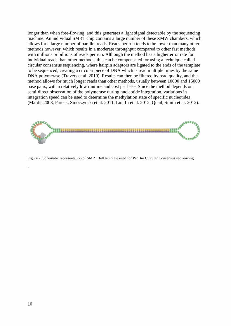
Figure 2. Schematic representation of SMRTBell template used for PacBio Circular Consensus sequencing.

¨

11

1.5 Aim of study

The goals of the project were:

1. Design and test out bar-coded primers for E. coli housekeeping genes from two different

MLST schemes.

2. Develop a higher throughput methodology to allow for the typing of hundreds of E. coli

samples.

3. Amplify and sequence the selected E. coli housekeeping genes from DNA isolated from

fecal samples from a human infant, taken at frequent intervals between ages 0 and 12 months.

4. Identify, categorize, and quantify E. coli strain types in the samples using the sequencing

data, and determine how the strain composition and relative abundance of the gut changes

over time, as well as identifying potential environmental factors or phenotypic properties that

might contribute to such changes of the composition of the microbiome.

This project is related to previous work done by Eric de Muinck, where he compared

the strain composition of E. coli in the gut microbiome of a group of human infants over five

time points (2d, 4d, 10day, 4months, and two years)(de Muinck et al. 2011). The

methodology developed here allows for MLST typing in a multiplexed format of at least one

hundred samples per PacBio sequencing run. In this thesis we applied this methodology to

follow fine scale E. coli changes over time in a single infant over the first year of life. This

can be considered a proof of concept for future research in which strain dynamics of many

different species of host bacteria can be followed in populations or in individuals at fine time

scales.

12

2 Experimental

2.1 Materials and reagents

All PCR reactions were performed using Phusion DNA Polymerase and Phusion HF

or GC Buffer from the Thermo Fisher Scientific Phusion High-Fidelity DNA Polymerase kit.

2 mM dNTP, MiliQ H2O, and 10 mg/ml BSA.

PCR results were visualized by electrophoresis on 1% Agarose gels with Gel Red

fluorescent DNA stain, run with 1x TAE buffer. Samples were loaded using Thermo Fisher

Scientific 6X Massruler loading dye, and results compared against Low Range Thermo Fisher

Scientific FastRuler DNA Ladder.

DNA concentrations were measured with a NanoDrop spectrophotometer. Before final

pooling of samples, DNA concentration was measured with a Qubit 2.0 fluorometer using

reagents from the Thermo Fisher Scientific Qubit dsDNA BR (Broad Range) assay kit.

Before submission for sequencing, pooled samples were purified using the Qiagen

QIAquick PCR Purification kit, together with 96% ethanol and 3M sodium acetate.

2.1.1 Samples and standards

For the PCR reactions, DNA isolates from strains in the ECOR collection were used as

template for the positive controls. The strains used were: ECOR 19, 31, 34, 40, 42, 43, 60, 66,

and 69. In addition fecal DNA from a healthy adult isolated using the Qiagen Stool Kit was

used as controls to test if the extraction protocol caused samples to contain contaminants that

might influence PCR.

After initial testing, 16S primers 806r and 515f (Caporaso et al. 2012) were used as a

control for all samples.

2.1.2 DNA isolates

Fecal samples were collected over one year from a healthy newborn infant according

to REK agreement (2014/656). Samples were immediately frozen at -20°C pending transfer to

a long term storage facility at -80°C. Total DNA from fecal samples was extracted using the

MO BIO PowerSoil 96 well DNA isolation kit.

13

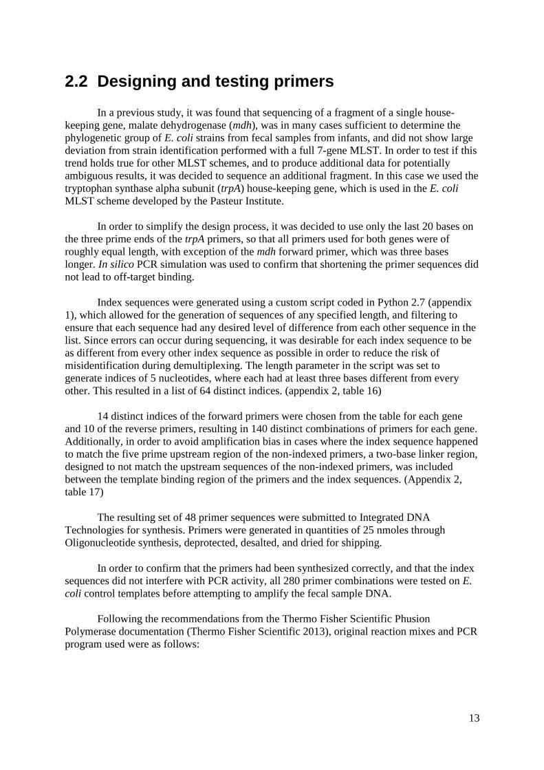
2.2 Designing and testing primers

In a previous study, it was found that sequencing of a fragment of a single house-

keeping gene, malate dehydrogenase (mdh), was in many cases sufficient to determine the

phylogenetic group of E. coli strains from fecal samples from infants, and did not show large

deviation from strain identification performed with a full 7-gene MLST. In order to test if this

trend holds true for other MLST schemes, and to produce additional data for potentially

ambiguous results, it was decided to sequence an additional fragment. In this case we used the

tryptophan synthase alpha subunit (trpA) house-keeping gene, which is used in the E. coli

MLST scheme developed by the Pasteur Institute.

In order to simplify the design process, it was decided to use only the last 20 bases on

the three prime ends of the trpA primers, so that all primers used for both genes were of

roughly equal length, with exception of the mdh forward primer, which was three bases

longer. In silico PCR simulation was used to confirm that shortening the primer sequences did

not lead to off-target binding.

Index sequences were generated using a custom script coded in Python 2.7 (appendix

1), which allowed for the generation of sequences of any specified length, and filtering to

ensure that each sequence had any desired level of difference from each other sequence in the

list. Since errors can occur during sequencing, it was desirable for each index sequence to be

as different from every other index sequence as possible in order to reduce the risk of

misidentification during demultiplexing. The length parameter in the script was set to

generate indices of 5 nucleotides, where each had at least three bases different from every

other. This resulted in a list of 64 distinct indices. (appendix 2, table 16)

14 distinct indices of the forward primers were chosen from the table for each gene

and 10 of the reverse primers, resulting in 140 distinct combinations of primers for each gene.

Additionally, in order to avoid amplification bias in cases where the index sequence happened

to match the five prime upstream region of the non-indexed primers, a two-base linker region,

designed to not match the upstream sequences of the non-indexed primers, was included

between the template binding region of the primers and the index sequences. (Appendix 2,

table 17)

The resulting set of 48 primer sequences were submitted to Integrated DNA

Technologies for synthesis. Primers were generated in quantities of 25 nmoles through

Oligonucleotide synthesis, deprotected, desalted, and dried for shipping.

In order to confirm that the primers had been synthesized correctly, and that the index

sequences did not interfere with PCR activity, all 280 primer combinations were tested on E.

coli control templates before attempting to amplify the fecal sample DNA.

Following the recommendations from the Thermo Fisher Scientific Phusion

Polymerase documentation (Thermo Fisher Scientific 2013), original reaction mixes and PCR

program used were as follows:

14

Tables 1-3. Recipes for PCR reaction mixes of different volumes, and PCR program used in initial experiments.

Alterations to the reaction mix and PCR program are noted as they were implemented

in the testing regimen. To streamline reaction setup, master mixes were made containing all

reagents except for primers and template, multiplied by the number of reactions in the

experiment, and distributed into the PCR tubes. Template and primers were added to

individual tubes as dictated by the experiment setup. After PCR, 10 μl of PCR product mixed

with 2 μl Massruler loading dye (Thermo Fisher Scientific 2012) for each reaction was loaded

onto separate wells on a 1% agarose gel, next to 5 μl Fastruler low range DNA ladder

(Thermo Fisher Scientific 2012). This was reduced to 5 μl of PCR product with 1 μl

Massruler loading dye after the first two experiments, as the excessive amount of DNA

loaded caused the bands to form large blobs rather than narrow bands when smaller wells

were used to run a higher number of samples per gel.

Elctrophoresis was performed at 100V for 30 minutes, and the resulting bands were

visualized using the Syngene GeneGenius BIO imaging system.

In the first experiment, the primer combination mdh Forward 1/Reverse 1 was

compared to unindexed mdh primers as a positive control. For each primer combination, four

50 μl reactions were prepared: For each of the temples, ECOR66 and ECOR69, a reaction

with the template and a negative control without the template were prepared. Since the two

negative controls were identical, one was removed in future experiments as it was considered

redundant.

Reaction nr. 1 2 3 4 5 6 7 8

Primers MDH Control MDH F1-R1

Template None ECOR66 None ECOR69 None ECOR66 None ECOR69

Table 4. Experimental setup for prototype primer testing scheme.

All negative controls displayed no bands during visualization. Test reactions had

strong bands in the 600-700 base pair region as expected, but the indexed primers had bands

indicating smaller fragments as well. These were thought to be caused by primer dimerization

1x 50 μl PCR reaction mix

MiliQ H2O 27,5μl

5x HF buffer 10μl

2mM dNTP 5μl

10μM Forward primer 2,5μl

10μM Reverse primer 2,5μl

Phusion DNA

Polymerase

0,5μl

Template DNA 2μl

1x 20 μl PCR reaction mix

MiliQ H2O 10,8μl

5x HF buffer 4μl

2mM dNTP 2μl

10μM Forward primer 1μl

10μM Reverse primer 1μl

Phusion DNA

Polymerase

0,2μl

Template DNA 1μl

PCR program

Denaturation 98oC 30 seconds

30 cycles: 98 oC 10 seconds

55 oC 30 seconds

72 oC 30 seconds

Final extension 72 oC 7 minutes

Hold 10 oC Indefinitely

15

or other non-specific hybridization due to suboptimal annealing temperatures, since the ideal

temperature had yet to be confirmed experimentally. (appendix 3, figure 16)

Using a similar setup, primer combinations MDH F2-R2, F3-R3, F4-R4, and F5-R5

were tested with ECOR66 and ECOR69 as templates, using the unindexed mdh primers as a

control, and having one negative control for each primer combination. All negative controls

showed no bands, positive controls displayed bands of expected size as previously, and the

test reactions displayed expected bands and smaller bands as in the previous experiment.

(appendix 3, figure 17.)

In order to test all primer permutations in a reasonable time frame, a massive

upscaling of the experiment was performed: Each run consisted of a multiple of 16 reactions,

comprising forward primers 1-14 with a specific reverse primer, and a negative and positive

control with the unindexed primer. For each set of 16 reactions, DNA from a randomly picked

ECOR isolate was used as template, as the primers should ideally work regardless of the

strain used, and the supply of individual DNA isolates was limited.

First run with the large scale setup covered all combinations for mdh reverse 1, reverse

2, and reverse 3. For reverse 1 and 3 sets, all test reactions displayed expected bands, and

negative control displayed no bands, and positive control displayed expected band. For the

reverse 2 set, multiple test reactions showed no bands, and the negative control had a band in

the same range as the positive control. This was attributed to pipetting error, and the set was

redone as part of the next run. (appendix 3, figure 18.)

Second run with the large scale setup covered all combinations for mdh reverse 2,

reverse 4, reverse 5, reverse 6, and reverse 7. All positives displayed expected bands, and all

negative controls displayed no bands. All test reactions displayed expected bands except for

the following: F11-R4, and F13-R7. (appendix 3, figure 19.)

Third run with the large scale setup covered all combinations for mdh reverse 8, and

all combinations for trpA reverse 1-8. Since no unindexed primers were available for trpA, the

following primers were used as controls:

For reverse 1 set, F8-R1,

For reverse 2 set, F8-R2,

For reverse 3-6 sets, F2-R2,

6 has no negative control,

For reverse 7, no controls,

For reverse 8, F5-R8.

The majority of the samples produced the expected bands, with the following

exceptions:

TrpA F8-R1, F1-R6, F13-R6, and F6-R7 displayed none or weak bands. The latter half

of R8 displayed no bands, possibly due to low amounts of loading dye while the samples were

loaded onto the gel. Due to a pipetting error, both positive and negative controls for trpA

reverse 3 and reverse 4 contain template. (appendix 3, figure 20.)

16

In the next run, the trpA reverse 8 set was run again on the agarose gel. In addition, the

PCRs were performed again for the following primer combinations that had previously failed:

mdh F11-R4, mdh F13-R7, trpA F7-R1, trpA F1-R6, trpA F13-R6, trpA F6-R7. Finally, to

check if contaminants in DNA isolated from fecal samples rather than pure cultures would

interfere with PCR, randomly picked primers for mdh and trpA were tested using increasing

concentrations (1, 2, 3, and 4 μl) of two fecal DNA samples, P1 and P2, attained from a

healthy adult and isolated using the Qiagen Stool Kit. Unindexed primers were used for

positive and negative controls for mdh, while the trpA set only had a negative control.

Of all the redone tests, the only ones not successful were trpA F1-R6 and trpA F13-R6.

It was decided that 110 successful primer combinations was sufficient to advance testing, and

to leave the testing of the reverse 9 and 10 primers for later should the need arise. From the

fecal DNA tests, P1 gave positive results across the board, though much weaker than from the

ECOR DNA, while P2 produced no bands in all cases. (appendix 3, figure 21.)

When beginning tests with actual sample material, it was decided to use 20 μl

reactions, due to limited availability of template. Due to decreased band strength with fecal

DNA, it was decided to increase the number of PCR cycles to 35, and to replace 0,8 μl of

H2O in the reaction mix with bovine serum albumin.

A set of randomly picked samples were tested against a set of randomly picked mdh

and trpA primers from the set of those confirmed to work with ECOR DNA. Unindexed mdh

primers were used as positive and negative controls, using one of the samples (Day 281) as

template. Positive control had one band of expected size, negative control had no bands.

(appendix 3, figure 22.)

Sample mdh primers mdh results TrpA primers TrpA results Day 226 F14R8 Smear F6R2 Band Day 214 F7R4 Faint bands F9R2 Faint band Day 225 F9R1 Band F7R3 Band Day 246 F13R6 Blank F1R8 Band Day 350 F10R7 Blank F9R4 Blank Day 359 F10R6 Faint bands - - Day 361 - - F2R6 Blank Day 281 F3R4 Band F6R6 Blank

Table 5. Experimental setup for test with randomly picked samples and primers.

In order to further increase amplification reliability, gradient PCR with annealing

temperatures between 50oC and 60

oC was performed using ECOR34 DNA diluted

hundredfold with mdh primers F1R1, and P1 fecal DNA trpA primers F1R1, in hope that

lower template concentrations would make the bands weak enough to pick an optimal upper

temperature. Despite this, the resulting bands were strong across the board, and did not show

significant decrease with higher annealing temperatures, as would be expected. However, off-

target products like primer dimerization decreased with increasing temperatures, and it was

decided to increase the annealing temperature to 58oC in future runs. (appendix 3, figure 23.)

In order to estimate the lower detection limit of the primers, a ten-fold dilution series

of ECOR34 DNA, starting at 1 and ending at 1/10000000, was used as templates for mdh

F1R1, trpA F1R1, and 16S primers 515F and 806r. For mdh, band strength dropped

17

significantly at 1/1000000 dilution, while in trpA and 16S a similar drop occurred at 1/100000

dilution. Using Nanodrop, starting concentration for DNA in the ECOR34 solution was

measured to be ~28ng/μl. (appendix 3, figure 24.)

Based on this, the lower detection limit for the mdh primers is estimated to be in the region of

0,028μg/μl, while the lower detection limit for the trpA and 16S primers is estimated to be in

the region of 0,28μg/μl

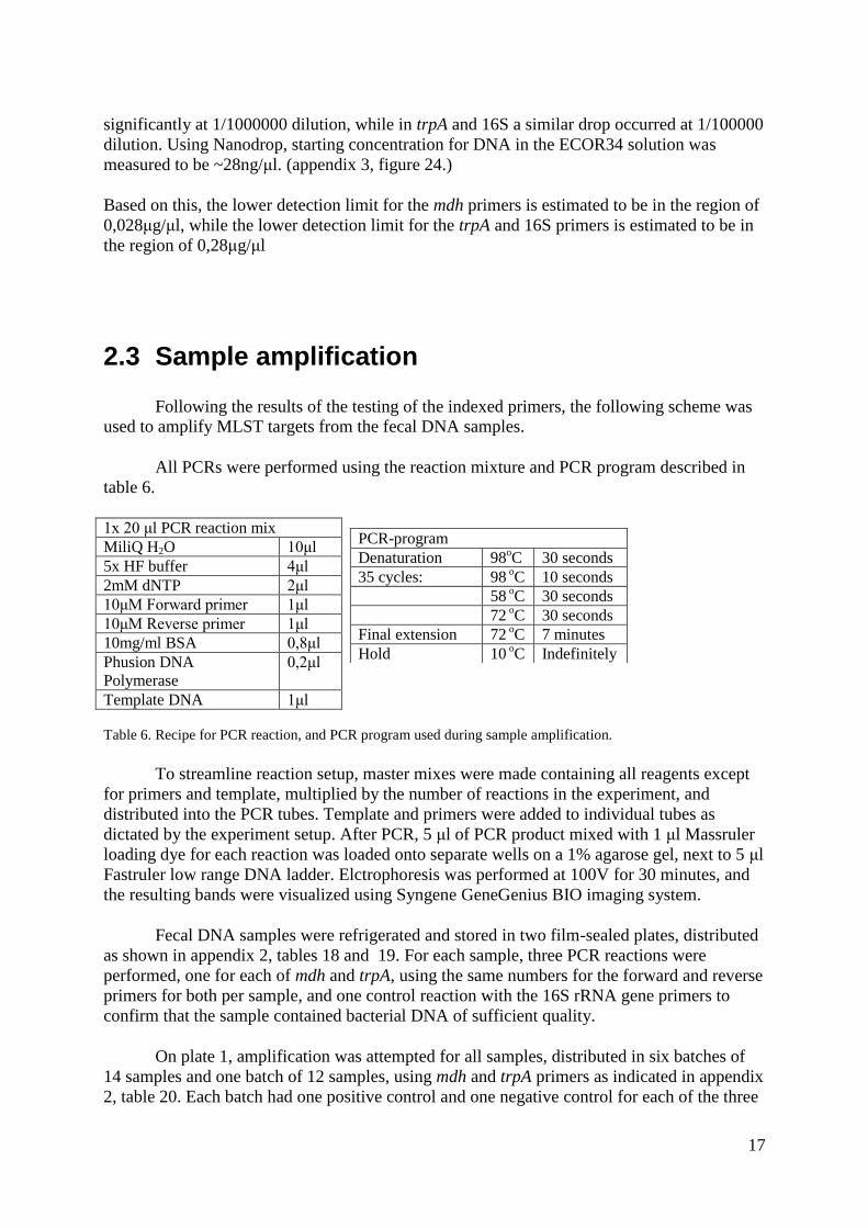
2.3 Sample amplification

Following the results of the testing of the indexed primers, the following scheme was

used to amplify MLST targets from the fecal DNA samples.

All PCRs were performed using the reaction mixture and PCR program described in

table 6.

1x 20 μl PCR reaction mix

MiliQ H2O 10μl

5x HF buffer 4μl

2mM dNTP 2μl

10μM Forward primer 1μl

10μM Reverse primer 1μl

10mg/ml BSA 0,8μl

Phusion DNA

Polymerase

0,2μl

Template DNA 1μl

Table 6. Recipe for PCR reaction, and PCR program used during sample amplification.

To streamline reaction setup, master mixes were made containing all reagents except

for primers and template, multiplied by the number of reactions in the experiment, and

distributed into the PCR tubes. Template and primers were added to individual tubes as

dictated by the experiment setup. After PCR, 5 μl of PCR product mixed with 1 μl Massruler

loading dye for each reaction was loaded onto separate wells on a 1% agarose gel, next to 5 μl

Fastruler low range DNA ladder. Elctrophoresis was performed at 100V for 30 minutes, and

the resulting bands were visualized using Syngene GeneGenius BIO imaging system.

Fecal DNA samples were refrigerated and stored in two film-sealed plates, distributed

as shown in appendix 2, tables 18 and 19. For each sample, three PCR reactions were

performed, one for each of mdh and trpA, using the same numbers for the forward and reverse

primers for both per sample, and one control reaction with the 16S rRNA gene primers to

confirm that the sample contained bacterial DNA of sufficient quality.

On plate 1, amplification was attempted for all samples, distributed in six batches of

14 samples and one batch of 12 samples, using mdh and trpA primers as indicated in appendix

2, table 20. Each batch had one positive control and one negative control for each of the three

PCR-program

Denaturation 98oC 30 seconds

35 cycles: 98 oC 10 seconds

58 oC 30 seconds

72 oC 30 seconds

Final extension 72 oC 7 minutes

Hold 10 oC Indefinitely

18

types of primer. The primers for the controls were mdh F1R1, trpA F1R1, and 16S 515F

806R. Negative controls had no template, and positive controls used the P1 fecal DNA as a

template.

The last of these batches also included two mock-samples, the first one using just

ECOR34 DNA as template, the second one using a 50/50 mix of ECOR34 and ECOR42 DNA

as template. These were made to help estimate the degree to which sequencing results would

indicate the relative abundance of different strains within a sample.

In order to determine how well the samples covered the time period of the study, the

number of successful amplifications for mdh and trpA were counted and visualized in figures

3 and 4. Full results of the sample amplifications can be found in appendix 2, table 22.

Figure 3. Distribution of samples from which mdh fragments were successfully amplified over the

weeks of the study.

Figure 4. Distribution of samples from which trpA fragments were successfully amplified over the

weeks of the study.

0

1

2

3

4

1 4 7 10 13 16 19 22 25 28 31 34 37 40 43 46 49 52

Po

siti

ve s

amp

les

Week

mdh

mdh

0

1

2

3

4

1 4 7 10 13 16 19 22 25 28 31 34 37 40 43 46 49 52

Po

siti

ve s

amp

les

Week

trpA

trpA

19

Based on this mapping, nine samples were picked from plate 2, from days not within

the weeks covered by the successfully amplified samples from plate 1, and amplified using

the same scheme as the batches described above. Sample IDs and primers used are found in

appendix 2, table 21. Amplification was reattempted for samples where only one gene had

been successfully amplified. Final set of samples to be included in the sequencing pool is

shown in table 7.

Sample day mdh trpA Sample day mdh trpA

9 ✓ ✓ 230 ✓ ✓

18 ✓ 237 ✓

26 ✓ 239 ✓ ✓

31 ✓ ✓ 244 ✓ ✓

41 ✓ 247 ✓ ✓

45 ✓ 256 ✓ ✓

57 ✓ ✓ 258 ✓ ✓

68 ✓ ✓ 267 ✓ ✓

74 ✓ ✓ 270 ✓

79 ✓ ✓ 280 ✓ ✓

96 ✓ ✓ 284 ✓ ✓

105 ✓ ✓ 287 ✓ ✓

112 ✓ ✓ 328 ✓ ✓

126 ✓ 329 ✓ ✓

143 ✓ ✓ 334 ✓ ✓

187 ✓ ✓ 337 ✓ ✓

196 ✓ ✓ 349 ✓ ✓

209 ✓ ✓ 351 ✓ ✓

214 ✓ 357 ✓ ✓

215 ✓ ✓ 362 ✓

218 ✓ ✓ Custom sample 1 ✓ ✓

223 ✓ ✓ Custom sample 2 ✓ ✓

Table 7. Final set of samples to be included in the sequencing pool

2.4 Pooling and purification

In order to prepare for sequencing, the selected samples had to be pooled together in

volumes according to their relative DNA concentrations, to ensure that each sample would be

equally represented in the sequencing data. The resulting sample pool then had to be purified

to remove contaminants that might interfere with sequencing.

DNA concentrations in the selected samples were measured using a Qubit 2.0

Fluorometer with the Qubit double stranded DNA Broad Range assay kit, as described in the

manual (Thermo Fisher Scientific 2015).

For all readings, sample assay tubes were prepared with 2μl sample and 198μl Qubit

working solution.

20

The optimal total amount of DNA in the purified sequencing pool for the sequencing

reaction was 1000ng, and it was estimated that about half the DNA would be lost during

purification. As such, the desired amount of DNA from each of the 78 samples before

purification would be 2000ng/78 ≈ 25ng.

Table 8 shows the calculated DNA concentration for each sample, as well as the

volume added to the sequencing pool. For samples where the desired volume was lower than

1 μl, values are represented as fractions where the numerator indicates the volume added and

the denominator indicates the degree of dilution with milliQ H2O.

Sample

day

mdh trpA Sample

day

mdh trpA

Cons

ng/μl

Volume

μl

Cons

ng/μl

Volume

μl

Cons

ng/μl

Volume

μl

Cons

ng/μl

Volume

μl 9 53.3 1/2 9.38 2.5 230 18.5 1.5 31.3 1

18 3.52 7 - - 237 7.76 3 - -

26 20.7 1 - - 239 43.0 3/5 62.3 2/5

31 5.16 5 6.02 4 244 19.1 1.5 12.9 2

41 27.3 1 - - 247 91.2 2/7 35.2 3/4

45 47.3 1/2 - - 256 8.71 3 27.3 1

57 105 1/4 12 2 258 161 1/6 29.9 1

68 4.57 5.5 8.17 3 267 39.8 3/5 18.4 1.5

74 18.1 1.5 10.1 2.5 270 60.7 4 - -

79 11.9 2 26.8 1 280 28.4 1 56.2 1/2

96 3.06 8 4.4 5.5 284 37.5 2/3 12.6 2

105 3.11 8 3.5 7 287 6.95 4 15.6 1.5

112 4.12 6 18.8 1.5 328 - - 53.6 1/2

126 5.05 5 - - 329 10.1 2.5 13.3 2

143 26.5 1 34.2 3/4 334 8.34 3 13.7 2

187 9.33 3 29.4 1 337 17.2 1.5 16.2 1.5

196 13.4 2 13.9 2 349 14.6 2 17.3 1.5

209 36.1 7 24.7 1 351 6.43 4 16.5 1.5

214 19.6 1.5 - - 357 39.4 2/3 101 1/4

215 8.35 3 20 1 362 4.02 6 - -

218 53.1 1/2

19.1 1.5 Custom

sample 1 110 1/4

236 1/10

223 51.9 1/2

59.2 2/5 Custom

sample 2 163 1/6

173 1/6

Table 8. Concentration and volume added for all samples in the sequencing pool. Samples marked in red were

added in tenfold higher volumes than intended due to a calculation error.

The pooled samples were purified using the QIAquick PCR Purification kit, as

described in the manual using the microcentrifuge protocol (Qiagen 2010). Elution was

performed using MiliQ H2O.

After purification, 5 μl of the sequencing pool was mixed with 1 μl Massruler loading

dye and loaded onto a 1% agarose gel, next to 5 μl Fastruler low range DNA ladder.

Electrophoresis was performed at 100V for 30 minutes, and the resulting bands were

visualized using the Syngene GeneGenius BIO imaging system.. (Shown in appendix 3,

figure 25.) As the visualization displays two distinct bands in the expected size ranges for

mdh and trpA, the sample pool was cleared for sequencing. 1μl was used to measure the DNA

concentration using a NanoDrop spectrophotometer and was found to be 24,4ng/μl.

21

2.5 Sequencing

44μl of the purified pooled samples, with estimated total DNA content of 1074ng, was

submitted for Single molecule real time sequencing on a Pacific Biosciences RS II sequencer

using a single SMRT cell.

The sequencing service was provided by the Norwegian Sequencing Centre

(www.sequencing.uio.no), a national technology platform hosted by the University of Oslo

and supported by the "Functional Genomics" and "Infrastructure" programs of the Research

Council of Norway and the Southeastern Regional Health Authorities.

Results were filtered by quality, and two fastq files were generated as output, one with

a quality cut-off of 90% accuracy, and one with a quality cut-off of 99% accuracy. Full

sequencing report can be found in appendix 4.

2.5.1 Filtering sequencing results

In order to separate the reads from the sequencing results by source sample, and to

count the number of identical reads within an individual sample, two workflows were made in

Lifeportal, a UiO maintained install of Galaxy running on the Abel high performance

computing cluster. Full workflows can be found at

https://lifeportal.uio.no/u/sigmunr%40uio.no/w/filtering-ecoli-pool-by-primer-sequences-mdh

and

https://lifeportal.uio.no/u/sigmunr%40uio.no/w/filtering-ecoli-pool-by-primer-sequences-trpa,

and a schematic representation of the demultiplexing process is shown in figure 5.

Figure 5. Schematic representation of the demultiplexing process performed in the Lifeportal workflows.

22

Because Lifeportal was not up to date with the development version of Galaxy when

these workflows were designed, they were not able to benefit from new features that allow for

more simple iteration over large numbers of datasets, such as Dataset Collections or Multiple

File Datasets. Because of this the workflows are quite unwieldy, and cannot easily be

modified to filter out other combinations of primers, or to filter by different primers or

indices. Although they can be used for technical replication of the analysis process, it is

recommended that future experiments create workflows on an updated version of Galaxy, use

a different platform altogether, or use existing demultiplexing pipelines.

Tools used in the workflow:

FastQ to FastA (v1.0.0)(Blankenberg et al. 2010), Revseq (6.5.7)(Blankenberg et al. 2007),

Collapse (0.0.13), Tabular-To-FASTA, FASTA-To-Tabular, Cut, Trim, Compare, Filter.

23

3 Results and discussion

3.1 Sample coverage

Fecal samples were collected by the subject's parents at semi-regular intervals over a

period of 365 days, or just over 52 weeks, starting with the the subject's date of birth.

Although the samples were only taken on 35,9% of the days during the year of the study, they

were distributed in such a way that there was at least one sample taken in 82,7% of the weeks

in the trial period. (Distribution of samples taken and sequenced over days and weeks shown

in table 9)

Category Nr. of days % of days Nr. of weeks % of weeks

Not sampled

234 64,1 9 17,3

Sampled but not

sequenced 90 24,7 9 17,3

Sampled and sequenced

for only one gene 10 2,7 7 13,5

Sampled and sequenced

for both genes 32 8,8 27 51,9

Table 9. Distribution of sample coverage over the days and weeks of the study period.

The nine weeks where no samples were taken were nr. 13, nr. 22-25, and nr. 43-46, the

latter two sets of weeks accounting for the two largest gaps in the resulting dataset. (A map of

the week by week sample coverage can be seen in figure 6.)

Additionally, weeks 17-20 only had one sample for mdh and none for trpA that were

successfully amplified and sequenced, which might be indicative of the E. coli DNA

concentration in the samples in this time period being below or close to the amplification limit

for the selected primers, or the samples contained some form of contaminant that interfered

with amplification. All samples within this time period were attempted amplified in separate

reactions on different days, and for all of them some of the other amplification reactions

performed the same day using the same reaction mixture and conditions were successful,

indicating that these failed amplifications were likely not caused by systematic errors during

amplification, but rather due to the properties of these particular samples.

Lastly, one sample, trpA day 230, was added to the sequencing pool, but no reads were

identified after demultiplexing. This might result from accidentally applying the incorrect

primers to the reaction mix during amplification, or from an error during the application of the

sample to the sequencing pool.

24

Figure 6. Distribution of samples and successful amplifications over the weeks of the study period.

3.2 Identifying strains

In order to reduce the interference of spurious sequences in the dataset, sequences that

appeared fewer than three times in a particular sample were not included in the analysis. The

remaining sequences were labelled by searching for the closest matching named allele in the

Shigatox and Pasteur MLST databases for mdh and trpA respectively. In order to test the

validity of this naming scheme, and to compare the read number and signal to noise ratio of

the 90% accuracy cut-off and 99% accuracy cut-off datasets, the alleles present for both genes

were first identified in the synthetic control samples, whose templates contained just reference

strain ECOR34 DNA or a 50/50 mix of ECOR34 and ECOR42 DNA.

Based on the MLST data for the ECOR reference strains in the Shigatox and Pasteur

MLST databases, the expected alleles for ECOR34 were mdh8 and trpA8, and for ECOR42

were mdh130 and trpA36. For both datasets, looking at the sequences with frequencies above

the cut-off limit, only the expected alleles were present in the sequencing data for each sample

(figures 7 and 8), but the samples with mixed templates heavily favoured the ECOR42

sequences. This indicated that ECOR42 was present at a higher relative frequency than

ECOR34. The difference in the number of sequences that appeared more than three times was

negligible between the two datasets, while there was a slight increase in the number of

sequences that appeared three or fewer times in the dataset using 90% accuracy as the cut-off

in the quality filtering, compared to the dataset using 99% accuracy as the cut-off, leading to a

slightly lower noise to signal ratio (table 10). Because of this, the 99% accuracy cut-off

dataset was used in all further analysis.

0

1

1 6 11 16 21 26 31 36 41 46 51 Sam

plin

g st

atu

s

Week

Sample coverage by week

Only one housekeeping gene sequenced

Both housekeeping genes sequenced

Sampled but not sequenced

25

Figure 7. Distribution of identified sequences in the synthetic mdh control samples using different levels of

quality filtering.

Figure 8. Distribution of identified sequences in the synthetic trpA control samples using different levels of

quality filtering.

Samples Identified sequences Discarded sequences Signal to noise ratio

mdh, 99% accuracy 266 203 1,31

trpA, 99% accuracy 283 312 0,91

mdh, 90% accuracy 275 233 1,18

trpA, 90% accuracy 284 369 0,77

Table 10. Signal to noise ratios for the synthetic samples under different levels of quality filtering.

26

Following this, sequences from all samples in the dataset were compared against the

named alleles in the Shigatox and Pasteur MLST databases, and the following alleles, or close

relatives thereof, were identified (table 11). For all sequences examined, there were either

found exact matches in the MLST databases, or closely resembled sequences with exact

matches that appeared more frequently in the same samples, suggesting that these represented

minor amplification or sequencing errors, rather than novel alleles.

mdh alleles trpA alleles

mdh 1 trpA 1

mdh 2 trpA 2

mdh 5 trpA 8

mdh 8 trpA 10

mdh 35 trpA 12

mdh 36 trpA 19

mdh 60 trpA 36

mdh 85 trpA 139

mdh 96

mdh 122

mdh 130 Table 11. Closest resembling alleles in MLST databases to sequence variants appearing in sequencing data.

In order to confirm if all the identified sequences were representative of different

strains, pairwise distance matrices were generated for both the mdh alleles and the trpA alleles

using the Maximum Composite Likelihood method in MEGA 7.0.14 (Appendix 2, table 23

and 24). If two allele sequences have a very high degree of similarity, are found

predominantly or exclusively in the same samples, and one has a lower frequency than the

other, this would be indicative of one of the sequences possibly being the result of misreads of

the other during sequencing, rather than coming from separate strains.

For the mdh alleles, the pairs displaying a very high degree of similarity were mdh2-

mdh8, mdh2-mdh122, and mdh35-mdh36. For the trpA alleles, the only pair displaying a very

high degree of similarity was trpA2-trpA10. For each of these pairs the number of samples

each allele was found in, and the number of samples where they appear together are listed in

table 12. (Full table of alleles found for each sample can be found in appendix 2, tables 25 and

26). Since both mdh2 and mdh8 both appear in multiple separate samples, it is safe to

conclude that these two alleles represent (at least) two different strains that are present in the

dataset. mdh122 and trpA10 may represent misreads of mdh2 and trpA2 respectively, but

since the number of reads for each are not very different within each sample, all four alleles

were retained as separate in further analysis. For mdh35 and mdh36, some of the reads in the

samples where both occur may result from sequencing errors, however, when comparing the

relative abundance of reads between the two alleles for each sample, it's found that each allele

is dominant in a different stretch of the trial period. (Days 196 to 230 for mdh36, and days

247 to 284 for mdh35). This suggests that the alleles represent (at least) two different strains

present in the dataset, and both are retained as separate for further analysis.

27

Allele pair Nr. Samples

with first allele

Nr. samples with

second allele

Nr. samples with

both alleles

mdh2

mdh8 8 7 1

mdh2 mdh122

8 2 2

Mdh35

mdh36 12 11 7

trpA2 trpA10

6 2 1

Table.12. Overlap and lack thereof for sequences with a high degree of similarity.

E. coli strains are commonly divided into five phylogenetic groups: A, B1, B2, D, and

E (Carlos et al. 2010). In order to better characterize the different sequences found in the

sequencing data, phylogenetic groups were assigned to the alleles using a method based on

previous work by Eric de Muinck (de Muinck, Øien et al. 2011). Using the mdh and trpA

sequences from the Shigatox and Pasteur MLST databases for all ECOR reference strains to

provide a phylogenetic framework, (with the exception of ECOR51 mdh, which was not

represented by an isolate in the Shigatox database,) phylogenetic trees were generated with

the sample alleles for both mdh and trpA by Maximum Likelihood using MEGA 7.0.14

(Figures 9 and 10). As expected based on the results of the previous study, sequences divide

broadly into the expected phylogenetic groups, but with a number of misassigned sequences,

due to loss of information in single gene typing versus multi gene typing. Because of this, and

due to placement of sample alleles between the established phylogenetic groups in some

cases, there is some ambiguity in the assignment of phylogenetic groups for some alleles.

Assigned phylogenetic groups for all alleles can be found in table 13.

Figures 9 and 10. Phylogenetic analysis of mdh and trpA strains. The evolutionary history was inferred by using the Maximum Likelihood

method based on the Tamura-Nei model. The trees with the highest log likelihoods are shown. Initial tree(s) for the heuristic search were

obtained automatically by applying Neighbor-Join and BioNJ algorithms to a matrix of pairwise distances estimated using the Maximum

Composite Likelihood (MCL) approach, and then selecting the topology with superior log likelihood value. The tree is drawn to scale, with

branch lengths measured in the number of substitutions per site. Codon positions included were 1st+2nd+3rd+Noncoding. All positions

containing gaps and missing data were eliminated. Evolutionary analyses were conducted in MEGA7 (Tamura et al. 1993, Kumar et al.

2016).

28

mdh alleles Phylogenetic group trpA alleles Phylogenetic group

mdh 1 A trpA 1 A

mdh 2 A or B1 trpA 2 B2

mdh 5 B1 trpA 8 B1

mdh 8 B1 trpA 10 B2

mdh 35 B2 trpA 12 D

mdh 36 B2 trpA 19 B2 or D

mdh 60 E trpA 36 B1 or E

mdh 85 B1 trpA 139 E

mdh 96 D

mdh 122 A or B1

mdh 130 E Table 13. Assigned phylogenetic groups for all identified alleles in the sequencing data.

29

3.3 Mapping strain distribution

For the majority of the samples for both mdh and trpA, the total numbers of

sequencing reads per sample was somewhere below 500 reads, with two major exceptions;

mdh day 209, with 1075 reads, and mdh day 270, with 712 reads. As noted in the Pooling and

Purification section, these two samples were added to the sequencing pool in tenfold higher

volumes than intended, due to a calculation error. These two samples alone account for

respectively 11,4% and 7,6% of the 9425 reads that could successfully be traced back to

specific samples. In the ideal case, where each sample was represented equally in the

sequencing data, the expected value would be 1,3%, or roughly 120 reads per sample.

Figures 11 and 12. Mapping of read numbers per day over the study period for both mdh and trpA datasets.

30

The distribution of alleles identified per sample over the year of the sample is shown

in figure 13 for mdh, and figure 14 for trpA. (Read numbers for all samples can be found in

appendix 2, tables 25 and 26). The strain composition can be divided into five blocks of

relative stability, beginning and ending with short transitional periods with higher strain

diversity, or during periods with no sampling data:

1. Days 9-79: During this period, the alleles found in mdh samples fluctuates between mdh1,

or mdh8 and mdh130 coexisting. trpA coverage is scarce during this early period, but the only

allele identified in most of the samples in this period was trpA1. The end of this first block is

marked by the sudden appearance of mdh2 and trpA36, and the first week with no samples

taken.

2. Days 96-143: During the entirety of this period, only one allele was detected for both mdh

and trpA: mdh1 and trpA1. This continues to the end of the block, which is marked by the first

of the two month long periods during which no samples were taken.

3. Days 187-244: At the beginning of this period on day 187, the following alleles were

identified: mdh2, mdh5, mdh60 trpA8 and trpA10. From day 196 to 230, the dominant alleles

found were mdh36 and trpA2, with sporadic appearances of mdh5, mdh8, and mdh35. At the

end of the block, the dominant allele was replaced by a mix of mdh2, mdh5, mdh8, mdh36,

mdh60, and trpA80.

4. Days 247-287: Following the transitional period at the end of the previous block, the

dominant alleles found in this block were mdh35 and trpA19, with sporadic appearances of

mdh36 and trpA8. At the end of the block, the dominant allele was replaced by mdh2,

mdh122, trpA1 and trpA8, followed by the second month long period during which no

samples were taken.

5. Days 329-362: At the beginning of this block, between day 329 and 337, a large number of

different alleles were identified: mdh2, mdh5, mdh8 mdh35, mdh36, mdh85, mdh96, mdh122,

trpA1, trpA8, and trpA12. From day 349 to the end of the study period, the dominant alleles

were mdh60 and trpA139.

31

Figures 13 and 14. Mapping of allele distribution per day over the study period for both mdh and trpA datasets.

The four blocks where single mdh and trpA alleles were identified, were postulated to

represent single strains, or a number of very closely related strains, which were designated

with the letters A to D as shown in table 14.

Designation mdh allele Time period trpA allele Time period

A mdh 1 Day 96-143 trpA 1 Day 96-143

B mdh 36 Day 196-230 trpA 2 Day 196-223

C mdh 35 Day 247-284 trpA 19 Day 247-284

D mdh 60 Day 349-362 trpA 139 Day 349-357 Table14. Designations of suspected dominant strains present in sequencing data for both genes.

32

In order to categorize these strains into phylogenetic groups, concatenated sequences

were generated for all ECOR reference strains except ECOR51, by attaching the sequences of

their trpA alleles to their mdh alleles from the Shigatox and Pasteur databases, head to tail.

These were used to provide a phylogenetic framework, and the concatenated sequences of the

sample strains were mapped onto a phylogenetic tree generated by Maximum Likelihood

using MEGA 7.0.14 (Figure 15). The tree generated using the sequences of both genes

together matched the expected distribution of ECOR strains into the five phylogenetic groups

better than either of the trees generated using one of the genes alone (figures 9 and 10), with

only five strains not falling neatly into the expected distributions (ECOR28, ECOR42, ECOR

43, ECOR58, and ECOR66).

Sample strains were categorized by their position in the phylogenetic tree, and

categorization matched with the one performed single genes for both mdh and trpA (Table

15).

Figure 15. Phylogenetic analysis of combined MLST data for trpA and mdh. The evolutionary history was inferred by using the

Maximum Likelihood method based on the Tamura-Nei model. The tree with the highest log likelihood (-3105.2307) is shown.

Initial tree(s) for the heuristic search were obtained automatically by applying Neighbor-Join and BioNJ algorithms to a matrix of

pairwise distances estimated using the Maximum Composite Likelihood (MCL) approach, and then selecting the topology with

33

superior log likelihood value. The tree is drawn to scale, with branch lengths measured in the number of substitutions per site.

The analysis involved 75 nucleotide sequences. Codon positions included were 1st+2nd+3rd+Noncoding. All positions

containing gaps and missing data were eliminated. There were a total of 1110 positions in the final dataset. Evolutionary

analyses were conducted in MEGA7 (Tamura and Nei 1993, Kumar, Stecher et al. 2016).

Designation Phylogenetic group predicted

with both mdh and trpA

Phylogenetic group

predicted with mdh

Phylogenetic group

predicted with trpA

A A A A

B B2 B2 B2

C B2 or D B2 B2 or D

D E E E Table15.Comparison of phylogenetic group assignment between combined gene and single-gene phylogenetic

analysis.

3.4 Metadata and environmental factors

In order to protect the identity of the subject and keep the study blind, the parents of

the subject were questioned about significant events, travel, antibiotics use and sickness,

using Eric de Muinck as a proxy to anonymize the data. The parents were also asked to make

note of events around the dates marking the beginning and end of the blocks identified in the

section Mapping Strain Distribution: Days 79, 96, 143, 187, 244, 287, and 329.

The subject was vaccinated on days 99, 200, and 362. All of these days fall within the

stable sections of blocks with single dominant strains, after the strain has been established,

and do not seem to have any immediate effect on strain composition.

Neither the subject not their mother used antibiotics during the year of the study, and

no instances of disease were noted by the parents.

The subject's diet began to include solid foods sometimes around days 88-95, which

matches with the transition between blocks 1 and 2, and the transition may be caused by this

change in diet.

It was noted that the longer time periods in which no samples were taken occurred as a

result of travel during the study year. Both blocks 3 and 5 follow directly from extended time

periods without sampling, and begin with short periods of high strain diversity, before it

stabilizes into the dominant strains.

While these observations suggest, as expected, that major changes in the gut

microbiome composition generally happen as a result of changes in environmental factors

such as diet and travel, it is difficult to make more detailed conclusions or predictions without

having similarly detailed datasets for multiple subjects to compare.

34

3.5 Strain properties

Of the five phylogenetic groups of E. coli A and B2 are the ones most commonly

found in the human microbiome by global average distribution, appearing as dominant in

40.5% and 25.5% of cases respectively.(Tenaillon, Skurnik et al. 2010) However, the exact

rates of dominance for reach group varies from country to country, and previous studies on

Norwegian and Swedish infants suggest that B2 is the predominant early colonizer of the

infant gut microbiome in these populations, to which the subject belongs. In spite of this, the

alleles found in samples from the early microbiome of the subject belonged predominantly to

group A, along with B1 and E, and B2 did not become the dominant strain until

approximately half a year into the study.

Although phylogenetic group E is known to contain enterohaemorragic strains, (such

as many of the O157:H7 serotype strains,) the link between phylogenetic distance and

pathology is small(Gordon et al. 2003), and no disease was noted by the parents during block

5, where a group E strain was dominant. Since previous studies suggest that group E strain

dominance is rare in early colonization of Scandinavian infants, (0.4% of infants in the 2011

study) (de Muinck, Øien et al. 2011), its presence in block 5 gives further credence to the idea

that the last observed shift in the population structure of the subject's microbiome resulted

from changes in environment during travel.

35

3.6 Scalability of experimental design

In order to adapt the methodology described in this paper to a larger study comparing

the microbiome of multiple infants, it would be necessary to amplify and sequence a much

larger number of samples (for ideal coverage of one sample per week for a whole year, 52

samples per gene amplified per infant). The most expensive processing step in this procedure

is the SMRT sequencing, and as such it would be desirable to have the largest number of

samples per sequencing reaction that would still produce viable data.

Using the exact primers designed for this project, the largest number of distinct

samples that could theoretically be sequenced in the same reaction would be 140 per gene (14

distinct forward primers and 10 distinct reverse primers). When generating index sequences

using the script described in appendix 1, it is possible to generate 64 distinct index sequences

5 nucleotides long where each is at least three bases different from every other in the set,

which were the same parameters used while picking sequences for this project. If no indices

are reused between reverse and forward primers, this allows for a maximum of 1024

combinations without reducing the difference threshold or increasing sequence length while

designing index sequences. As such, primer design should not be considered a limiting factor

in multiplexing.

According to the sequencing report, the one SMRT cell used in this project returned

46842 reads, of which 26290 (56%) passed 0.99 minimum accuracy filtering. Of these, 9425

could be assigned to specific samples, and 6307 were deemed to be of sufficient quality to be

used in strain categorization. If these rates are assumed to be representative for an average run

using this methodology, the average expected number of usable reads per sample if running

104 samples (52 per gene for two genes) on a single SMRT cell is 6307/104 ≈ 60. Because of

this, unless the signal to noise ratio is significantly improved, it is not recommended to

sequence sample sets from more than one subject per SMRT cell, and higher sample volumes

have to be handled by using higher numbers of SMRT cells per sequencing run.

36

4 Conclusion

The methodology described and tested in this thesis allows for the mapping of the

dynamics of the developing infant gastrointestinal microbiome at a much higher resolution

than previous studies, and is suitable for use in future studies comparing the microbiomes of

multiple infants, though further optimization is desirable to reduce the amount of malformed

or junk reads. This increased resolution will potentially allow for the tracing of changes in the

gut microbiome to specific environmental factors, and provide greater understanding of the

normal development of the neonatal microbiome in healthy infants, and how changes in strain

composition occurs. Using multiple genes from different MLST schemes allows for more

accurate classification of ambiguous strains, although this is limited to dominant strains

unless pure cultures are generated from the sample material.

The study was able to sample 43 of the 52 weeks of the study period, determine five

timespans with different dominant E. coli strains, identify potential environmental factors

relating to travel and changes in diet that might be linked to the changes between these

periods, and classify multiple competing strains during periods where the strain composition

of the gut microbiome is undergoing changes. Alleles suggesting the presence of at least 11

different strains colonizing the gut microbiome of the subject during the study period were

identified. This is a larger number than similar previous studies, and can be explained by the

much higher sample coverage.

37

5 Appendix

Appendix 1: Primer-index generating script

print "Length of index sequences?"

indexlength = raw_input()

inxlen = int(indexlength)

print "Minimum nr. of different bases?"

difference = raw_input()

diff = inxlen - int(difference)

indexlist=[]

bases="ATGC"

testlist = ["A","T","G","C"]

progress = 2

while progress <= inxlen:

templist = []

for seq in testlist:

for base in bases:

templist.append(seq+base)

testlist = templist

progress = progress + 1

for teststring in testlist:

print "Checking " + teststring

maxsimilarity = 0

for index in indexlist:

pos = 0

similarity = 0

while pos <= inxlen-1:

if index[pos] == teststring[pos]:

similarity = similarity + 1

pos = pos + 1

if similarity > maxsimilarity:

maxsimilarity = similarity

if maxsimilarity > diff:

print "Too similar"

else:

print "Added"

indexlist.append(teststring)

print "Final list:"

print indexlist

length1 = len(indexlist)

length2 = str(length1)

print length2 + " indexes found."

saveq = 0

while saveq == 0:

saveoutput = raw_input ("Save output to file? y/n: ")

if "y" in saveoutput.lower():

filename = raw_input ("File name? ") +".txt"

fo = open(filename, "w")

for index in indexlist:

fo.write ("%s\n" % index)

fo.close()

saveq = 1

elif "n" in saveoutput.lower():

saveq = 1

38

Appendix 2: Miscellaneous tables

AAAAA AATTT AAGGG AACCC ATATG ATTAC ATGCA ATCGT

AGAGC AGTCG AGGAT AGCTA ACACT ACTGA ACGTC ACCAG

TAATC TATAG TAGCT TACGA TTAAT TTTTA TTGGC TTCCG

TGACA TGTGT TGGTG TGCAC TCAGG TCTCC TCGAA TCCTT

GAAGT GATCA GAGAC GACTG GTACC GTTGG GTGTT GTCAA

GGAAG GGTTC GGGGA GGCCT GCATA GCTAT GCGCG GCCGC

CAACG CATGC CAGTA CACAT CTAGA CTTCT CTGAG CTCTC

CGATT CGTAA CGGCC CGCGG CCAAC CCTTG CCGGT CCCCA Table 16. Index sequences generated during primer design.

Primer

name

Sequence Primer

name

Sequence Primer

name

Sequence Primer

name

Sequence

MDH

fw1

AAAAAGAG

TCGATCTG

AGCCATAT

CCCTAC

MDH

rv1

ACACTGC

TACTGAC

CGTCGCC

TTCAAC

TRPA

fw1

TTAATTG

GCTACGA

ATCTCTG

TTTGCC

TRPA

rv1

GAAGTGG

GCTTTCAT

CGGTTGT

ACAAA

MDH

fw2

AATTTGAG

TCGATCTG

AGCCATAT

CCCTAC

MDH

rv2

ACTGAGC

TACTGAC

CGTCGCC

TTCAAC

TRPA

fw2

TTTTATG

GCTACGA

ATCTCTG

TTTGCC

TRPA

rv2

GATCAGG

GCTTTCAT

CGGTTGT

ACAAA

MDH

fw3

AAGGGGAG

TCGATCTG

AGCCATAT

CCCTAC

MDH

rv3

ACGTCGC

TACTGAC

CGTCGCC

TTCAAC

TRPA

fw3

TTGGCTG

GCTACGA

ATCTCTG

TTTGCC

TRPA

rv3

GAGACGG

GCTTTCAT

CGGTTGT

ACAAA

MDH

fw4

AACCCGAG

TCGATCTG

AGCCATAT

CCCTAC

MDH

rv4

ACCAGGC

TACTGAC

CGTCGCC

TTCAAC

TRPA

fw4

TTCCGTG

GCTACGA

ATCTCTG

TTTGCC

TRPA

rv4

GACTGGG

GCTTTCAT

CGGTTGT

ACAAA

MDH

fw5

ATATGGAG

TCGATCTG

AGCCATAT

CCCTAC

MDH

rv5

TAATCGC

TACTGAC

CGTCGCC

TTCAAC

TRPA

fw5

TGACATG

GCTACGA

ATCTCTG

TTTGCC

TRPA

rv5

GTACCGG

GCTTTCAT

CGGTTGT

ACAAA

MDH

fw6

ATTACGAG

TCGATCTG

AGCCATAT

CCCTAC

MDH

rv6

TATAGGC

TACTGAC

CGTCGCC

TTCAAC

TRPA

fw6

TGTGTTG

GCTACGA

ATCTCTG

TTTGCC

TRPA

rv6

GTTGGGG

GCTTTCAT

CGGTTGT

ACAAA

MDH

fw7

ATGCAGAG

TCGATCTG

AGCCATAT

CCCTAC

MDH

rv7

TAGCTGC

TACTGAC

CGTCGCC

TTCAAC

TRPA

fw7

TGGTGTG

GCTACGA

ATCTCTG

TTTGCC

TRPA

rv7

GTGTTGG

GCTTTCAT

CGGTTGT

ACAAA

MDH

fw8

ATCGTGAG

TCGATCTG

AGCCATAT

CCCTAC

MDH

rv8

TACGAGC

TACTGAC

CGTCGCC

TTCAAC

TRPA

fw8

TGCACTG

GCTACGA

ATCTCTG

TTTGCC

TRPA

rv8

GTCAAGG

GCTTTCAT

CGGTTGT

ACAAA

MDH

fw9

AGAGCGAG

TCGATCTG

AGCCATAT

CCCTAC

MDH

rv9

GGGGAGC

TACTGAC

CGTCGCC

TTCAAC

TRPA

fw9

TGCACTG

GCTACGA

ATCTCTG

TTTGCC

TRPA

rv9

GCGCGGG

GCTTTCAT

CGGTTGT

ACAAA

39

MDH

fw10

AGTCGGAG

TCGATCTG

AGCCATAT

CCCTAC

MDH

rv10

GGCCTGC

TACTGAC

CGTCGCC

TTCAAC

TRPA

fw10

TCTCCTG

GCTACGA

ATCTCTG

TTTGCC

TRPA

rv10

GCCGCGG

GCTTTCAT

CGGTTGT

ACAAA

MDH

fw11

AGGATGAG

TCGATCTG

AGCCATAT

CCCTAC

TRPA

fw11

TCGAATG

GCTACGA

ATCTCTG

TTTGCC

MDH

fw12

AGCTAGAG

TCGATCTG

AGCCATAT

CCCTAC

TRPA

fw12

TCCTTTG

GCTACGA

ATCTCTG

TTTGCC

MDH

fw13

GGAAGGAG

TCGATCTG

AGCCATAT

CCCTAC

TRPA

fw13

GCATATG

GCTACGA

ATCTCTG

TTTGCC

MDH

fw14

GGTTCGAG

TCGATCTG

AGCCATAT

CCCTAC

TRPA

fw14

GCTATTG

GCTACGA

ATCTCTG

TTTGCC

Table 17. Sequences of all primers designed for this project

1 2 3 4 5 6 7 8 9 10 11 12

A PC1 223 334 287 229 269 PC2 361 359 262 12 74

B NC 357 349 211 350 222 272 236 263 248 200 45

C 216 239 330 225 226 258 270 238 212 363 69 196

D 218 227 351 245 210 237 281 282 261 67 185 23

E 280 231 329 285 256 345 209 331 249 62 79 143

F 328 247 215 265 241 365 198 337 230 122 26 41

G 214 284 275 267 256 257 283 244 213 141 31 57

H 242 362 187 288 352 217 289 246 279 139 9 PC3

Table 18. Plate 1 map, sampling days

1 2 3 4 5 6

A PC1 112 14 76 182 105

B NC 199 8 64 77 19

C 51 38 18 73 197 128

D 55 142 180 113 61

E 191 188 1 192 21

F 33 192 126 130 68

G 16 75 10 131 35

H 66 22 11 96 71

Table 19. Plate 2 map, sampling days

40

1 2 3 4 5 6 7 8 9 10 11 12

A F1R1

F9 R1

F6 R2

F14 R2

F8 R3

F2 R4

F10 R4

F4 R5

F12 R5

F7 R6

F2 R7

F10 R7

B F2R1

F10 R1

F7 R2

F1 R3

F9 R3

F3 R4

F11 R4

F5 R5

F13 R5

F8 R6

F3 R7

F11 R7

C F3R1

F11 R1

F8 R2

F2 R3

F10 R3

F4 R4

F12 R4

F6 R5

F14 R5

F9 R6

F4 R7

F12 R7

D F4R1

F12 R1

F9 R2

F3 R3

F11 R3

F5 R4

F13 R4

F7 R5

F2 R6

F10 R6

F5 R7

F13 R7

E F5R1

F13 R1

F10 R2

F4 R3

F12 R3

F6 R4

F14 R4

F8 R5

F3 R6

F11 R6

F6 R7

F14 R7

F F6R1

F14 R1

F11 R2

F5 R3

F13 R3

F7 R4

F1 R5

F9 R5

F4 R6

F12 R6

F7 R7

F1 R8

G F7R1

F3 R2

F12 R2

F6 R3

F14 R3

F8 R4

F2 R5

F10 R5

F5 R6

F14 R6

F8 R7

F2 R8

H F8R1

F4 R2

F13 R2

F7 R3

F1 R4

F9 R4

F3 R5

F11 R5

F6 R6

F1 R7

F9 R7

F3 R8

Table 20. Plate 1 map, primer combinations for both mdh and trpA

1 2 3 4 5 6

A - F6 R8 - - -

F14 R8

B - - - - - -

C - - F7 R8 - - -

D - - F8 R8 - - -

E - - F9 R8 - - -

F - - F10 R8 -

F13 R8

-

G - - - F11 R8 - -

H - - - F12 R8 - -

Table 21. Plate 2 map, primer combinations for both mdh and trpA

Day mdh

results trp

results 16s

results Day mdh

results trp

results 16s

results Day mdh

results trp

results 16s

results

1 0 0 0 131 0 0 0 247 1 1 1

8 139 0 0 0 248 0 0 0

9 1 0 0 141 0 0 1 249 0 0 1

10 142 256 1 0 1

11 143 1 1 0 256 1 1 1

12 0 0 1 180 0 0 0 257 0 0 0

14 182 258 1 1 0

16 185 0 0 0 261 0 0 1

18 1 0 0 187 1 1 1 262 0 0 0

19 188 263 0 0 0

21 191 265 0 0 1

22 192 267 0 1 1

23 0 0 0 192 269 1 0 1

26 1 0 0 196 3 0 0 270 1 0 0

31 1 0 0 197 272 0 0 0

33 198 0 0 0 275 0 0 1

35 199 279 0 0 0

38 200 0 0 0 280 1 1 1

41 1 0 0 209 1 1 0 281 0 0 0

45 1 0 0 210 1 1 1 282 0 0 1

51 211 1 0 0 283 0 1 0

55 212 0 1 0 284 1 1 1

57 1 0 0 213 0 0 0 285 1 1 1

61 214 0 0 1 287 3 0 1

62 0 0 1 215 1 1 1 288 0 0 1

64 216 0 0 0 289 0 0 0

66 217 1 0 0 328 0 1 1

67 0 0 1 218 1 0 1 329 1 0 1

68 1 1 1 222 0 0 1 330 1 0 0

69 0 0 1 223 1 1 1 331 0 0 1

71 225 1 0 0 334 1 0 1

41

73 226 0 1 1 337 1 0 1

74 1 1 0 227 0 1 1 345 0 0 0

75 229 0 0 1 349 1 3 1

76 230 1 1 0 350 0 0 0

77 231 3 1 1 351 1 1 1

79 0 1 0 236 0 0 1 352 1 0 1

96 1 1 1 237 1 0 0 357 1 1 1

105 1 1 1 238 0 0 1 359 1 0 0

112 1 1 1 239 0 1 1 361 0 0 0

113 241 0 0 1 362 1 0 1

122 0 0 1 242 0 1 1 363 0 0 1

126 1 0 0 244 1 0 1 365 0 0 0

128 245 0 0 0

Table 22. Results of initial amplification attempts for all sample. 1 indicates successful amplification. 0 indicates

unsuccessful amplification or ambiguous results. Blank indicates amplification was not attempted.

mdh1 mdh2 mdh5 mdh8 mdh35 mdh36 mdh60 mdh85 mdh96 mdh122 mdh130

mdh1 0,000 0,009 0,013 0,009 0,017 0,017 0,023 0,015 0,017 0,013 0,017

mdh2 0,009 0,000 0,007 0,004 0,011 0,011 0,013 0,009 0,007 0,004 0,011

mdh5 0,013 0,007 0,000 0,011 0,019 0,019 0,021 0,002 0,015 0,011 0,019

mdh8 0,009 0,004 0,011 0,000 0,015 0,015 0,017 0,013 0,011 0,007 0,015

mdh35 0,017 0,011 0,019 0,015 0,000 0,004 0,021 0,020 0,015 0,011 0,015

mdh36 0,017 0,011 0,019 0,015 0,004 0,000 0,021 0,020 0,015 0,011 0,015

mdh60 0,023 0,013 0,021 0,017 0,021 0,021 0,000 0,023 0,017 0,017 0,021

mdh85 0,015 0,009 0,002 0,013 0,020 0,020 0,023 0,000 0,017 0,013 0,021

mdh96 0,017 0,007 0,015 0,011 0,015 0,015 0,017 0,017 0,000 0,011 0,011

mdh122 0,013 0,004 0,011 0,007 0,011 0,011 0,017 0,013 0,011 0,000 0,015

mdh130 0,017 0,011 0,019 0,015 0,015 0,015 0,021 0,021 0,011 0,015 0,000 Table 23. Pairwise-distance matrix for mdh alleles computed using the maximum composite likelihood model in

MEGA7.

trpA_1 trpA_2 trpA_8 trpA_10 trpA_12 trpA_19 trpA_36 trpA_139

trpA_1 0,000 0,062 0,009 0,064 0,062 0,067 0,011 0,031

trpA_2 0,062 0,000 0,064 0,004 0,043 0,026 0,062 0,048

trpA_8 0,009 0,064 0,000 0,066 0,062 0,069 0,009 0,033

trpA_10 0,064 0,004 0,066 0,000 0,043 0,025 0,064 0,050

trpA_12 0,062 0,043 0,062 0,043 0,000 0,035 0,062 0,060

trpA_19 0,067 0,026 0,069 0,025 0,035 0,000 0,066 0,054

trpA_36 0,011 0,062 0,009 0,064 0,062 0,066 0,000 0,035

trpA_139 0,031 0,048 0,033 0,050 0,060 0,054 0,035 0,000 Table 24. Pairwise-distance matrix for trpA alleles computed using the maximum composite likelihood model in

MEGA7.

Primers F9R7 F7R8 F7R7 F8R7 F1R8 F11R7 F2R8 F13R8 F10R7 F6R7 F12R8 F14R8 F6R8

Sample number 85 109 83 84 91 87 92 128 86 82 122 131 99

Day 9 18 26 31 41 45 57 68 74 79 96 105 112

mdh 1 0 12 0 0 0 0 86 17 0 0 18 81 85

mdh 2 0 0 0 0 0 0 0 0 0 28 0 0 0

mdh 35 0 0 0 0 0 0 0 0 0 0 0 0 0

mdh 36 0 0 0 0 0 0 0 0 0 0 0 0 0

mdh 5 0 0 0 0 0 0 0 0 0 0 0 0 0

mdh 60 0 0 0 0 0 0 0 0 0 0 0 0 0

mdh 8 4 0 18 0 0 21 0 0 0 0 0 0 0

mdh 85 0 0 0 0 0 0 0 0 0 0 0 0 0

mdh 96 0 0 0 0 0 0 0 0 0 0 0 0 0

mdh 122 0 0 0 0 0 0 0 0 0 0 0 0 0

mdh 130 20 0 48 39 6 10 0 0 10 0 0 0 0

Junked reads 11 14 22 6 2 8 22 7 5 22 15 37 35

Total 35 26 88 45 8 39 108 24 15 50 33 118 120

42

Primers F14R7 F13R2 F12R7 F14R4 F7R1 F11R2 F4R1 F9R1 F4R6 F5R4 F11R1 F10R5 F14R1

Sample number 90 22 88 50 5 20 2 7 67 42 9 60 12

Day 143 187 196 209 214 215 218 223 230 237 239 244 247

mdh 1 206 0 0 0 0 0 0 0 0 0 0 0 0

mdh 2 0 17 0 0 0 0 0 0 0 23 5 8 0

mdh 35 0 0 9 0 0 0 0 7 4 8 0 0 99

mdh 36 0 0 10 785 171 55 24 20 9 0 0 0 0

mdh 5 0 25 0 0 0 8 0 0 0 0 17 0 0

mdh 60 0 19 0 0 0 0 0 0 0 0 15 0 0

mdh 8 0 0 0 0 0 0 0 0 6 0 0 7 0

mdh 85 0 0 0 0 0 0 0 0 0 0 0 0 0

mdh 96 0 0 0 0 0 0 0 0 0 0 0 0 0

mdh 122 0 0 0 0 0 0 0 0 0 0 0 0 0

mdh 130 0 0 0 0 0 0 0 0 0 0 0 0 0

Junked reads 49 64 10 290 81 55 39 32 15 49 232 19 93

Total 255 125 29 1075 252 118 63 59 34 80 269 34 192

Primers F14R3 F4R4 F6R3 F12R4 F5R1 F3R2 F14R2 F10R2 F6R2 F9R5 F7R2 F9R2 F10R1

Sample number 37 41 29 48 3 13 23 19 15 59 16 18 8

Day 256 258 267 270 280 284 287 329 334 337 349 351 357

mdh 1 0 0 0 0 0 0 0 0 0 0 0 0 0

mdh 2 0 0 0 0 0 0 16 12 0 0 4 0 0

mdh 35 123 306 236 535 108 127 0 0 6 0 0 0 0

mdh 36 11 0 0 6 0 20 0 0 51 0 0 0 0

mdh 5 0 0 0 0 0 0 0 0 0 0 5 0 0

mdh 60 0 0 0 0 0 0 0 0 0 0 47 111 18

mdh 8 0 0 0 0 0 0 0 0 0 31 0 0 0

mdh 85 0 0 0 0 0 0 0 22 0 4 0 0 0

mdh 96 0 0 0 0 0 0 0 9 0 0 0 0 0

mdh 122 0 0 0 0 0 0 12 8 0 0 0 0 0

mdh 130 0 0 0 0 0 0 0 0 0 0 0 0 0

Junked reads 42 87 55 171 72 60 23 23 39 19 122 30 59

Total 176 393 291 712 180 207 51 74 96 54 178 141 77

Primers F4R2 F4R8 F5R8

Sample number 14 Cust.1 Cust.2

Day 362

mdh 1 0 0 0

mdh 2 0 0 0

mdh 35 0 0 0

mdh 36 0 0 0

mdh 5 0 0 0

mdh 60 78 0 0

mdh 8 0 112 24

mdh 85 0 0 0

mdh 96 0 0 0

mdh 122 0 0 0

mdh 130 0 0 130

Junked reads 36 28 175

Total 114 140 329

Table 25. Number of reads of each mdh sequence variant identified for each sample.

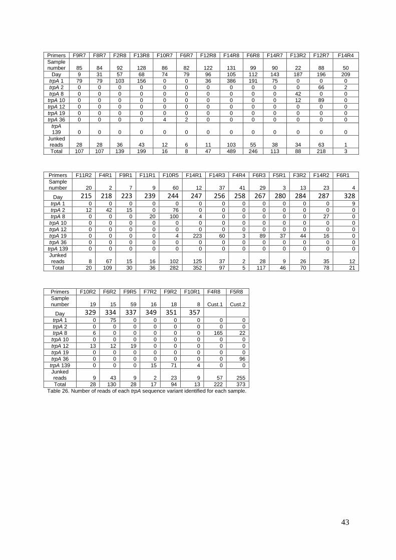
43

Primers F9R7 F8R7 F2R8 F13R8 F10R7 F6R7 F12R8 F14R8 F6R8 F14R7 F13R2 F12R7 F14R4

Sample number 85 84 92 128 86 82 122 131 99 90 22 88 50

Day 9 31 57 68 74 79 96 105 112 143 187 196 209

trpA 1 79 79 103 156 0 0 36 386 191 75 0 0 0

trpA 2 0 0 0 0 0 0 0 0 0 0 0 66 2

trpA 8 0 0 0 0 0 0 0 0 0 0 42 0 0

trpA 10 0 0 0 0 0 0 0 0 0 0 12 89 0

trpA 12 0 0 0 0 0 0 0 0 0 0 0 0 0

trpA 19 0 0 0 0 0 0 0 0 0 0 0 0 0

trpA 36 0 0 0 0 4 2 0 0 0 0 0 0 0

trpA 139 0 0 0 0 0 0 0 0 0 0 0 0 0

Junked reads 28 28 36 43 12 6 11 103 55 38 34 63 1

Total 107 107 139 199 16 8 47 489 246 113 88 218 3

Primers F11R2 F4R1 F9R1 F11R1 F10R5 F14R1 F14R3 F4R4 F6R3 F5R1 F3R2 F14R2 F6R1

Sample number 20 2 7 9 60 12 37 41 29 3 13 23 4

Day 215 218 223 239 244 247 256 258 267 280 284 287 328 trpA 1 0 0 0 0 0 0 0 0 0 0 0 0 9

trpA 2 12 42 15 0 76 0 0 0 0 0 0 0 0

trpA 8 0 0 0 20 100 4 0 0 0 0 0 27 0

trpA 10 0 0 0 0 0 0 0 0 0 0 0 0 0

trpA 12 0 0 0 0 0 0 0 0 0 0 0 0 0

trpA 19 0 0 0 0 4 223 60 3 89 37 44 16 0

trpA 36 0 0 0 0 0 0 0 0 0 0 0 0 0

trpA 139 0 0 0 0 0 0 0 0 0 0 0 0 0

Junked reads 8 67 15 16 102 125 37 2 28 9 26 35 12

Total 20 109 30 36 282 352 97 5 117 46 70 78 21

Primers F10R2 F6R2 F9R5 F7R2 F9R2 F10R1 F4R8 F5R8

Sample number 19 15 59 16 18 8 Cust.1 Cust.2

Day 329 334 337 349 351 357

trpA 1 0 75 0 0 0 0 0 0

trpA 2 0 0 0 0 0 0 0 0

trpA 8 6 0 0 0 0 0 165 22

trpA 10 0 0 0 0 0 0 0 0

trpA 12 13 12 19 0 0 0 0 0

trpA 19 0 0 0 0 0 0 0 0

trpA 36 0 0 0 0 0 0 0 96

trpA 139 0 0 0 15 71 4 0 0

Junked reads 9 43 9 2 23 9 57 255

Total 28 130 28 17 94 13 222 373

Table 26. Number of reads of each trpA sequence variant identified for each sample.

44

Appendix 3: Visualization of gel electrophoresis of PCR products.

Figure 16. Prototype testing scheme with mdh F1-R1

Figure 17. Prototype testing scheme with mdh F2-R2, F3-R3, F4-R4, and F5-R5. The negative control or F4-R4

has swapped places with one of the positives due to a pipetting error.

Figure 18. Large-scale testing scheme with mdh R1, R2, and R3 combinations.

45

Figure 19. Large-scale testing scheme with mdh R2, R4, R5, R6 and R7 combinations.

Figure 20. Large-scale testing scheme with mdh R8, and trpA R1, R2, R3, R4, R5, R6, R7, and R8

combinations.

46

Figure 21. Large-scale testing scheme with trpA R8 combinations, fecal DNA controls, and redos from previous

runs.

Figure 22. Trial run using randomly picked primers and samples

Figure 23. Gradient PCR to determine optimal annealing temperature.

47

Figure 24. PCR of template dilution series to determine lower detection limit for primers.

Figure 25. Electrophoresis of purified sequencing pool.

48

Appendix 4: Sequencing report

49

6 References

Abdulkareem, I. H. (2014). "Biomedical techniques in translational studies: The journey so

far." Niger Med J 55(2): 99-105.

Berg, R. D. (1996). "The indigenous gastrointestinal microflora." Trends in microbiology

4(11): 430-435.

Bettelheim, K. and S. Lennox-King (1976). "The acquisition of Escherichia coli by new-born

babies." Infection 4(3): 174-179.

Blankenberg, D., A. Gordon, G. Von Kuster, N. Coraor, J. Taylor, A. Nekrutenko and T.

Galaxy (2010). "Manipulation of FASTQ data with Galaxy." Bioinformatics 26(14): 1783-

1785.

Blankenberg, D., J. Taylor, I. Schenck, J. He, Y. Zhang, M. Ghent, N. Veeraraghavan, I.

Albert, W. Miller, K. D. Makova, R. C. Hardison and A. Nekrutenko (2007). "A framework

for collaborative analysis of ENCODE data: making large-scale analyses biologist-friendly."

Genome Res 17(6): 960-964.

Bumgarner, R. (2013). "Overview of DNA microarrays: types, applications, and their future."

Curr Protoc Mol Biol Chapter 22: Unit 22 21.

Caporaso, J. G., C. L. Lauber, W. A. Walters, D. Berg-Lyons, J. Huntley, N. Fierer, S. M.

Owens, J. Betley, L. Fraser, M. Bauer, N. Gormley, J. A. Gilbert, G. Smith and R. Knight

(2012). "Ultra-high-throughput microbial community analysis on the Illumina HiSeq and

MiSeq platforms." ISME J 6(8): 1621-1624.

Carlos, C., M. M. Pires, N. C. Stoppe, E. M. Hachich, M. I. Sato, T. A. Gomes, L. A. Amaral

and L. M. Ottoboni (2010). "Escherichia coli phylogenetic group determination and its

application in the identification of the major animal source of fecal contamination." BMC

Microbiol 10: 161.

Caugant, D. A., B. R. Levin and R. K. Selander (1981). "Genetic diversity and temporal

variation in the E. coli population of a human host." Genetics 98(3): 467-490.

Chakrabarti, R. and C. E. Schutt (2001). "The enhancement of PCR amplification by low

molecular-weight sulfones." Gene 274(1-2): 293-298.

Dark, M. J. (2013). "Whole-genome sequencing in bacteriology: state of the art." Infect Drug

Resist 6: 115-123.

de Muinck, E. J., T. Øien, O. Storrø, R. Johnsen, N. C. Stenseth, K. S. Rønningen and K. Rudi

(2011). "Diversity, transmission and persistence of Escherichia coli in a cohort of mothers and

their infants." Environmental microbiology reports 3(3): 352-359.

Farell, E. M. and G. Alexandre (2012). "Bovine serum albumin further enhances the effects of

organic solvents on increased yield of polymerase chain reaction of GC-rich templates." BMC

Res Notes 5: 257.

Foxman, B., L. Zhang, J. S. Koopman, S. D. Manning and C. F. Marrs (2005). "Choosing an

appropriate bacterial typing technique for epidemiologic studies." Epidemiol Perspect Innov

2: 10.

Freter, R., H. Brickner, J. Fekete, M. M. Vickerman and K. E. Carey (1983). "Survival and

implantation of Escherichia coli in the intestinal tract." Infection and immunity 39(2): 686-

703.

Google. (1986). "Patent; Process for amplifying, detecting, and/or-cloning nucleic acid

sequences." Retrieved May, 2016, from http://www.google.co.jp/patents/US4683195.

Gordon, D. M. and A. Cowling (2003). "The distribution and genetic structure of Escherichia

coli in Australian vertebrates: host and geographic effects." Microbiology 149(Pt 12): 3575-

3586.

50

Gordon, D. M. and A. Cowling (2003). "The distribution and genetic structure of Escherichia

coli in Australian vertebrates: host and geographic effects." Microbiology 149(12): 3575-

3586.

Grimont, F. and P. A. Grimont (1986). "Ribosomal ribonucleic acid gene restriction patterns

as potential taxonomic tools." Ann Inst Pasteur Microbiol 137B(2): 165-175.

Gritz, E. C. and V. Bhandari (2015). "The human neonatal gut microbiome: a brief review."

Front Pediatr 3: 17.

Herzer, P. J., S. Inouye, M. Inouye and T. S. Whittam (1990). "Phylogenetic distribution of

branched RNA-linked multicopy single-stranded DNA among natural isolates of Escherichia

coli." Journal of bacteriology 172(11): 6175-6181.

Johnson, J. K., S. M. Arduino, O. C. Stine, J. A. Johnson and A. D. Harris (2007).

"Multilocus sequence typing compared to pulsed-field gel electrophoresis for molecular

typing of Pseudomonas aeruginosa." J Clin Microbiol 45(11): 3707-3712.

Kleppe, K., E. Ohtsuka, R. Kleppe, I. Molineux and H. G. Khorana (1971). "Studies on

polynucleotides. XCVI. Repair replications of short synthetic DNA's as catalyzed by DNA

polymerases." J Mol Biol 56(2): 341-361.

Kumar, S., G. Stecher and K. Tamura (2016). "MEGA7: Molecular Evolutionary Genetics

Analysis Version 7.0 for Bigger Datasets." Mol Biol Evol.

Langhendries, J. P., T. Paquay, M. Hannon and J. Darimont (1998). "[Intestinal flora in the

neonate: impact on morbidity and therapeutic perspectives]." Arch Pediatr 5(6): 644-653.

Lee, P. Y., J. Costumbrado, C. Y. Hsu and Y. H. Kim (2012). "Agarose gel electrophoresis

for the separation of DNA fragments." J Vis Exp(62).

Liu, L., Y. Li, S. Li, N. Hu, Y. He, R. Pong, D. Lin, L. Lu and M. Law (2012). "Comparison

of next-generation sequencing systems." J Biomed Biotechnol 2012: 251364.

Maiden, M. C., J. A. Bygraves, E. Feil, G. Morelli, J. E. Russell, R. Urwin, Q. Zhang, J.

Zhou, K. Zurth, D. A. Caugant, I. M. Feavers, M. Achtman and B. G. Spratt (1998).

"Multilocus sequence typing: a portable approach to the identification of clones within

populations of pathogenic microorganisms." Proc Natl Acad Sci U S A 95(6): 3140-3145.

Maki, A., A. J. Rissanen and M. Tiirola (2016). "A practical method for barcoding and size-

trimming PCR templates for amplicon sequencing." Biotechniques 60(2): 88-90.

Mardis, E. R. (2008). "Next-generation DNA sequencing methods." Annu Rev Genomics

Hum Genet 9: 387-402.

Milkman, R. and M. M. Bridges (1990). "Molecular evolution of the Escherichia coli

chromosome. III. Clonal frames." Genetics 126(3): 505-517.

Mitsuoka, T. and K. Hayakawa (1973). "[The fecal flora in man. I. Composition of the fecal

flora of various age groups]." Zentralblatt fur Bakteriologie, Parasitenkunde,

Infektionskrankheiten und Hygiene. Erste Abteilung Originale. Reihe A: Medizinische

Mikrobiologie und Parasitologie 223(2): 333-342.

Neu, J. and J. Rushing (2011). "Cesarean versus vaginal delivery: long-term infant outcomes

and the hygiene hypothesis." Clin Perinatol 38(2): 321-331.

New England Biolabs. "PCR Protocol." Retrieved May, 2016, from

https://www.neb.com/protocols/1/01/01/pcr-protocol-m0530.

Nowrouzian, F., B. Hesselmar, R. Saalman, I.-L. Strannegård, N. Åberg, A. E. Wold and I.

Adlerberth (2003). "Escherichia coli in infants' intestinal microflora: colonization rate, strain

turnover, and virulence gene carriage." Pediatric research 54(1): 8-14.

Pacific Biosciences. (2015). "Barcoding training protocol." Retrieved May, 2015, from

https://github.com/PacificBiosciences/Bioinformatics-Training/wiki/Barcoding.

Parameswaran, P., R. Jalili, L. Tao, S. Shokralla, B. Gharizadeh, M. Ronaghi and A. Z. Fire

(2007). "A pyrosequencing-tailored nucleotide barcode design unveils opportunities for large-

scale sample multiplexing." Nucleic Acids Res 35(19): e130.

51

Pareek, C. S., R. Smoczynski and A. Tretyn (2011). "Sequencing technologies and genome

sequencing." J Appl Genet 52(4): 413-435.

Parracho, H., A. L. McCartney and G. R. Gibson (2007). "Probiotics and prebiotics in infant

nutrition." Proc Nutr Soc 66(3): 405-411.

Penders, J., C. Thijs, C. Vink, F. F. Stelma, B. Snijders, I. Kummeling, P. A. van den Brandt

and E. E. Stobberingh (2006). "Factors influencing the composition of the intestinal

microbiota in early infancy." Pediatrics 118(2): 511-521.

Poisson, D., J. Borderon, J. Amorim-Sena and J. Laugier (1986). "Evolution of the barrier

effects against an exogenous drug-sensitive Escherichia coli strain after single or repeated oral

administration to newborns and infants aged up to three months admitted to an intensive-care

unit." Neonatology 49(1): 1-7.

Qiagen. (2010). "Qiaquick protocol." Retrieved May, 2016, from

www.qiagen.com/literature/render.aspx?id=201082.

Quail, M. A., M. Smith, P. Coupland, T. D. Otto, S. R. Harris, T. R. Connor, A. Bertoni, H. P.

Swerdlow and Y. Gu (2012). "A tale of three next generation sequencing platforms:

comparison of Ion Torrent, Pacific Biosciences and Illumina MiSeq sequencers." BMC

Genomics 13: 341.

Saiki, R. K., D. H. Gelfand, S. Stoffel, S. J. Scharf, R. Higuchi, G. T. Horn, K. B. Mullis and

H. A. Erlich (1988). "Primer-directed enzymatic amplification of DNA with a thermostable

DNA polymerase." Science 239(4839): 487-491.

Schwartz, D. C. and C. R. Cantor (1984). "Separation of yeast chromosome-sized DNAs by

pulsed field gradient gel electrophoresis." Cell 37(1): 67-75.

Tamura, K. and M. Nei (1993). "Estimation of the number of nucleotide substitutions in the

control region of mitochondrial DNA in humans and chimpanzees." Mol Biol Evol 10(3):

512-526.

Tenaillon, O., D. Skurnik, B. Picard and E. Denamur (2010). "The population genetics of

commensal Escherichia coli." Nature Reviews Microbiology 8(3): 207-217.

Thermo Fisher Scientific. (2012). "Fastruler Protocol." Retrieved May, 2016, from

https://tools.thermofisher.com/content/sfs/manuals/MAN0013027_FastRuler_LowRange_DN

ALadder_RTU_UG.pdf.

Thermo Fisher Scientific. (2012). "Massruler protocol." Retrieved May, 2016, from

https://tools.thermofisher.com/content/sfs/manuals/MAN0011912_Prep_DNASmpls_Convent

ional_DNA_Electrophoresis_UG.pdf.

Thermo Fisher Scientific. (2013). "Phusion High Fidelity Polymerase Protocol." Retrieved

May, 2016, from

https://tools.thermofisher.com/content/sfs/manuals/MAN0012394_Phusion_HighFidelity_DN

APolymerase_100U_UG.pdf.

Thermo Fisher Scientific. (2015). "Qubit dsDNA BS Array Protocol." Retrieved May, 2016,

from https://tools.thermofisher.com/content/sfs/manuals/Qubit_dsDNA_BR_Assay_UG.pdf.

Touchon, M., C. Hoede, O. Tenaillon, V. Barbe, S. Baeriswyl, P. Bidet, E. Bingen, S.

Bonacorsi, C. Bouchier and O. Bouvet (2009). "Organised genome dynamics in the

Escherichia coli species results in highly diverse adaptive paths." PLoS genetics 5(1):

e1000344.

Travers, K. J., C. S. Chin, D. R. Rank, J. S. Eid and S. W. Turner (2010). "A flexible and

efficient template format for circular consensus sequencing and SNP detection." Nucleic

Acids Res 38(15): e159.