Embed Size (px)
Citation preview

Traffic grooming in bidirectional WDM ring networks∗
Jean-Claude Bermond 1 Xavier Munoz 2 Ignasi Sau 1,2
[email protected] [email protected] [email protected]
Version of July 11, 2010
Abstract
We study the minimization of ADMs (Add-Drop Multiplexers) in optical WDM bidirectionalrings considering symmetric shortest path routing and all-to-all unitary requests. We precisely for-mulate the problem in terms of graph decompositions, and state a general lower bound for all thevalues of the grooming factor C and N, the size of the ring. We first study exhaustively the casesC = 1, C = 2, and C = 3, providing improved lower bounds, optimal constructions for severalinfinite families, as well as asymptotically optimal constructions and approximations. We then studythe case C > 3, focusing specifically on the case C = k(k + 1)/2 for some k ≥ 1. We give optimal de-compositions for several congruence classes of N using the existence of some combinatorial designs.We conclude with a comparison of the cost functions in unidirectional and bidirectional WDM rings.
Keywords: Traffic grooming, SONET ADM, optical WDM network, graph decomposition, combi-natorial designs.
1 Introduction
1.1 Background and motivation
Optical wavelength division multiplexing (WDM) is today the most promising technology to accom-
modate the explosive growth of Internet and telecommunication traffic in wide-area, metro-area, and
backbone networks. Using WDM, the potential bandwidth of approximately 50 THz of a fiber can be
divided into multiple non-overlapping wavelength or frequency channels. Since currently the commer-
cially available optical fibers can support over a hundred frequency channels, such a channel has over
one gigabit-per-second transmission speed. However, the network is usually required to support traffic
1Mascotte joint Project I3S (CNRS/UNS) and INRIA - 2004, route des Lucioles - Sophia Antipolis, France.2Graph Theory and Combinatorics group at Applied Mathematics IV Department of UPC - Barcelona, Spain.∗An extended abstract of this article was presented at ICTON’06 [9]. This work was partially supported by European project
IST FET AEOLUS, by the Ministerio de Educacion y Ciencia, Spain, and the European Regional Development Fund underproject TEC2005-03575, by the Catalan Research Council under project 2005SGR00256 and by COST action 293.
1
2 Traffic grooming in bidirectional WDM ring networks
connections at rates that are lower than the full wavelength capacity. In order to save equipment cost
and improve network performance, it turns out to be very important to aggregate the multiple low-speed
traffic connections, namely requests, into higher speed streams. Traffic grooming is the term used to
carry out this aggregation, while optimizing the equipment cost.
Among possible criteria to minimize the equipment cost, one is to minimize the number of wave-
lengths used to route all the requests [2, 20]. A better approximation of the true equipment cost is to
minimize the number of add/drop locations, namely ADMs using SONET terminology, instead of the
number of wavelengths. This leads to the grooming problem, that we state formally later in Section 2.
These two problems are proved to be different. Indeed, it is known that even for a simple network like
the unidirectional ring, the number of wavelengths and the number of ADMs cannot be simultaneously
minimized [12, 23].
The SONET ring is the most widely used optical network infrastructure today. In these networks,
a communication between a pair of nodes is done via a lightpath, and each lightpath uses an Add-
Drop Multiplexer (ADM), i.e., an electronic termination, at each of its two endpoints (but none in the
intermediate nodes). If each request uses 1C of the capacity of a wavelength, then C is said to be the
grooming factor, i.e., C requests can be aggregated in the same wavelength through the same link. If two
or more lightpaths using the same wavelength share a common endpoint, then the same ADM might be
used for all lightpaths and therefore the number of ADMs needed could be reduced. Due to this fact, it
makes sense to try to minimize the total number of ADMs required.
1.2 Previous work and our contribution
The notion of traffic grooming was introduced in [25] for the ring topology. Since then, traffic grooming
has been widely studied in the literature (cf. [22,29,35] for some surveys). The problem has been proved
to be NP-complete for ring networks and general C [12]. Hardness results for rings and paths have been
proved in [1]. Many heuristics have been proposed, but exact solutions have been found only for certain
values of C and for the uniform all-to-all traffic case in unidirectional ring and path topologies [8].
Many versions of the problem can be considered, according for example to the routing, the physical
graph, and the request graph, among others. For example, in [3,6] the Path Traffic Grooming problem is
studied. If the network topology is a ring (which is the case of SONET rings), we mainly distinguish two
cases depending on the routing. The Unidirectional Ring Traffic Grooming problem has been studied
extensively in the literature. In an unidirectional ring, requests are routed following only one direction
in the cycle. To date, the all-to-all case has been completely solved for values of the grooming factor up
to 8 [4, 5, 8, 16, 17]. Also, recently the unidirectional ring with bounded degree request graph has been
studied [28, 30].
In the Bidirectional Ring Traffic Grooming problem, the scenario is quite different. In a bidirec-
tional ring, requests are routed either clockwise or counterclockwise. This case has been much less
studied than the unidirectional one, due to its higher complexity. There is important work providing
Jean-Claude Bermond, Xavier Munoz and Ignasi Sau 3
heuristics for the ring traffic grooming [11, 12, 20, 21, 23, 24, 27, 31], but there is still an important lack
of theoretical analysis of the problem. Nevertheless, its study has attracted the interest of numerous
researchers. For instance, in [26] a MILP formulation of the problem can be found. In [33] two lower
bounds are provided for the number of ADMs in a bidirectional ring with traffic grooming, and in [14]
another lower bound is proved, regardless of the routing. In [18, 19, 32, 33] tools from design theory are
applied to the bidirectional ring. Their method is based in the idea of primitive rings, which consists
roughly in appropriately generating subgraphs of the request graph inducing unitary load each, and then
packing them into sets of at most C subgraphs. Namely, in [33] several heuristics are proposed, the cases
C = 2 and C = 4 are studied in [32] (as well as other solutions that do not proceed via primitive rings),
the case C = 8 in [19], and the cases C = 4 and C = 8 in [18]. Nevertheless, they do not provide general
lower bounds and they do not analyze the approximation ratio of the proposed algorithms. Therefore,
the gaps between their solutions and the optimal ones are unknown.
In this work we focus on a bidirectional ring with symmetric shortest path routing, and on the all-to-
all case. We begin by formally stating the problem in terms of graph partitioning in Section 2. In Section
3 we provide lower bounds and compare them with those existing in the literature. The remainder of the
article is devoted to finding families of solutions for certain values of C and N. First we solve in Section 4
the case C = 1. In Section 5 we study the case C = 2, improving the general lower bound and providing
a 3433 -approximation. In Section 6 we tackle the case C = 3, improving the lower bound when N ≡ 3
(mod 4) and giving optimal solutions when N ≡ 0, 1, 4, 5 (mod 12). For all other values of N we give
asymptotically optimal solutions. In Section 7 we use design theory to provide optimal solutions when
C is of the form k(k + 1)/2, for some congruence classes of values of N. We also give improved lower
bounds when C is not of the form k(k + 1)/2. In Section 8 we compare unidirectional and bidirectional
rings in terms of minimizing the cost. We conclude the article in Section 9.
2 Statement of the Problem
2.1 Load constraint
In a graph-theoretical approach, we are given an optical network represented by a directed graph G on
N vertices (in many cases a symmetric one) – called the physical graph – for example a unidirectional
ring ~CN or a bidirectional symmetric ring C∗N . We are given also a traffic (or instance) matrix, that is
a family of connection requests represented by an arc-weighted multidigraph I – called the logical or
request graph – where the number of arcs from i to j corresponds to the number of requests from i to
j, and the weight of each arc corresponds to the amount of bandwidth used by each request. Here we
suppose that there is exactly one request from i to j (all-to-all case) and that each request uses the same
bandwidth. In that case I = K∗N . We also suppose that the bandwidth used by any request is a fraction
1/C of the available bandwidth of a wavelength. Said otherwise, each wavelength ω can carry on a given
arc at most C requests. This positive integer C is called the grooming factor. For a wavelength ω, we
4 Traffic grooming in bidirectional WDM ring networks
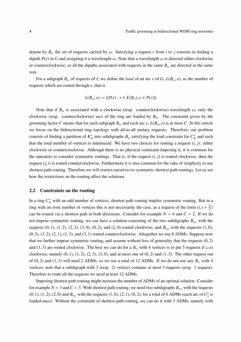
denote by Bω the set of requests carried by ω. Satisfying a request r from i to j consists in finding a
dipath P(r) in G and assigning it a wavelength ω. Note that a wavelength ω is directed either clockwise
or counterclockwise, so all the dipaths associated with requests in the same Bω are directed in the same
way.
For a subgraph Bω of requests of I, we define the load of an arc e of G, L(Bω, e), as the number of
requests which are routed through e, that is
L(Bω, e) := |{P(r) : r ∈ E(Bω), e ∈ P(r)}|.
Note that if Bω is associated with a clockwise (resp. counterclockwise) wavelength ω, only the
clockwise (resp. counterclockwise) arcs of the ring are loaded by Bω. The constraint given by the
grooming factor C means that for each subgraph Bω and each arc e, L(Bω, e) is at most C. In this article
we focus on the bidirectional ring topology with all-to-all unitary requests. Therefore, our problem
consists of finding a partition of K∗N into subdigraphs Bω satisfying the load constraint for C∗N and such
that the total number of vertices is minimized. We have two choices for routing a request (i, j): either
clockwise or counterclockwise. Although there is no physical constraint imposing it, it is common for
the operators to consider symmetric routings. That is, if the request (i, j) is routed clockwise, then the
request ( j, i) is routed counterclockwise. Furthermore it is also common for the sake of simplicity to use
shortest path routing. Therefore we will restrict ourselves to symmetric shortest path routings. Let us see
how the restrictions on the routing affect the solutions.
2.2 Constraints on the routing
In a ring C∗N with an odd number of vertices, shortest path routing implies symmetric routing. But in a
ring with an even number of vertices this is not necessarily the case, as a request of the form (i, i + N2 )
can be routed via a shortest path in both directions. Consider for example N = 4 and C = 2. If we do
not impose symmetric routing, we can have a solution consisting of the two subdigraphs Bω1 with the
requests (0, 1), (1, 2), (2, 3), (3, 0), (0, 2), and (2, 0) routed clockwise, and Bω2 with the requests (1, 0),
(0, 3), (3, 2), (2, 1), (1, 3), and (3, 1) routed counterclockwise. Altogether we use 8 ADMs. Suppose now
that we further impose symmetric routing, and assume without loss of generality that the requests (0, 2)
and (1, 3) are routed clockwise. The best we can do for a Bω with 4 vertices is to put 5 requests if ω is
clockwise, namely (0, 1), (1, 2), (2, 3), (3, 0), and at most one of (0, 2) and (1, 3). The other request out
of (0, 2) and (1, 3) will need 2 ADMs, so we use a total of 12 ADMs. If we do not use any Bω with 4
vertices, note that a subdigraph with 3 (resp. 2) vertices contains at most 3 requests (resp. 1 request).
Therefore to route all the requests we need at least 12 ADMs.
Imposing shortest path routing might increase the number of ADMs of an optimal solution. Consider
for example N = 3 and C = 3. With shortest path routing, we need two subdigraphs Bω1 with the requests
(0, 1), (1, 2), (2, 0) and Bω2 with the requests (1, 0), (2, 1), (0, 2), for a total of 6 ADMs (each arc of C∗3 is
loaded once). Without the constraint of shortest path routing, we can do it with 3 ADMs, namely with
Jean-Claude Bermond, Xavier Munoz and Ignasi Sau 5
all the requests routed clockwise. In that case, the requests (1, 0), (2, 1), and (0, 2) are routed via dipaths
of length 2 (for instance, the request (1, 0) uses the arcs (1, 2) and (2, 0)). In that case the load of the arcs
(in the clockwise direction) is 3.
We cannot always use shortest path routing and have a minimum load. Indeed, consider the case
C = 1 and a set of 3 requests (i, j), ( j, k), and (k, i) forming a triangle. The subdigraph formed by the
3 requests routed in the same direction has load 1, but there is no reason that the associated routes are
shortest paths. For example, let N = 5 and (0, 1), (1, 2), (2, 0) be the three mentioned requests, which we
assume to be routed clockwise. If we want a valid solution, then the request (2, 0) is routed via the path
[2, 3, 4, 0] of length 3 (and not 2). If we want to use shortest paths, then these three requests induce load
2, hence they cannot fit together in the same wavelength. Summarizing, in this example either we use
shortest paths and the load is 2 or we get a solution with load one but not using shortest paths.
2.3 Symmetric shortest path routing
In the sequel we will only consider symmetric shortest path routings. Besides being a common sce-
nario in telecommunication networks, this assumption also simplifies the problem, as we can split it into
two separate problems, half of the requests being routed clockwise and half counterclockwise. Each of
these two subproblems can be viewed as a grooming problem where G = ~CN (the unidirectional cycle)
and I = TN , where TN is a tournament on N vertices, that is, a complete oriented graph (for each pair of
vertices {i, j} there is exactly one of the arcs (i, j) or ( j, i)).
As we consider shortest path routing, for N odd TN is unique. But for N even we have two possibili-
ties for the pairs of the form {i, i + N2 }: either the arc (i, i + N
2 ) or (i + N2 , i). So the choice of these arcs has
to be made. We are now ready to precisely state our problem.
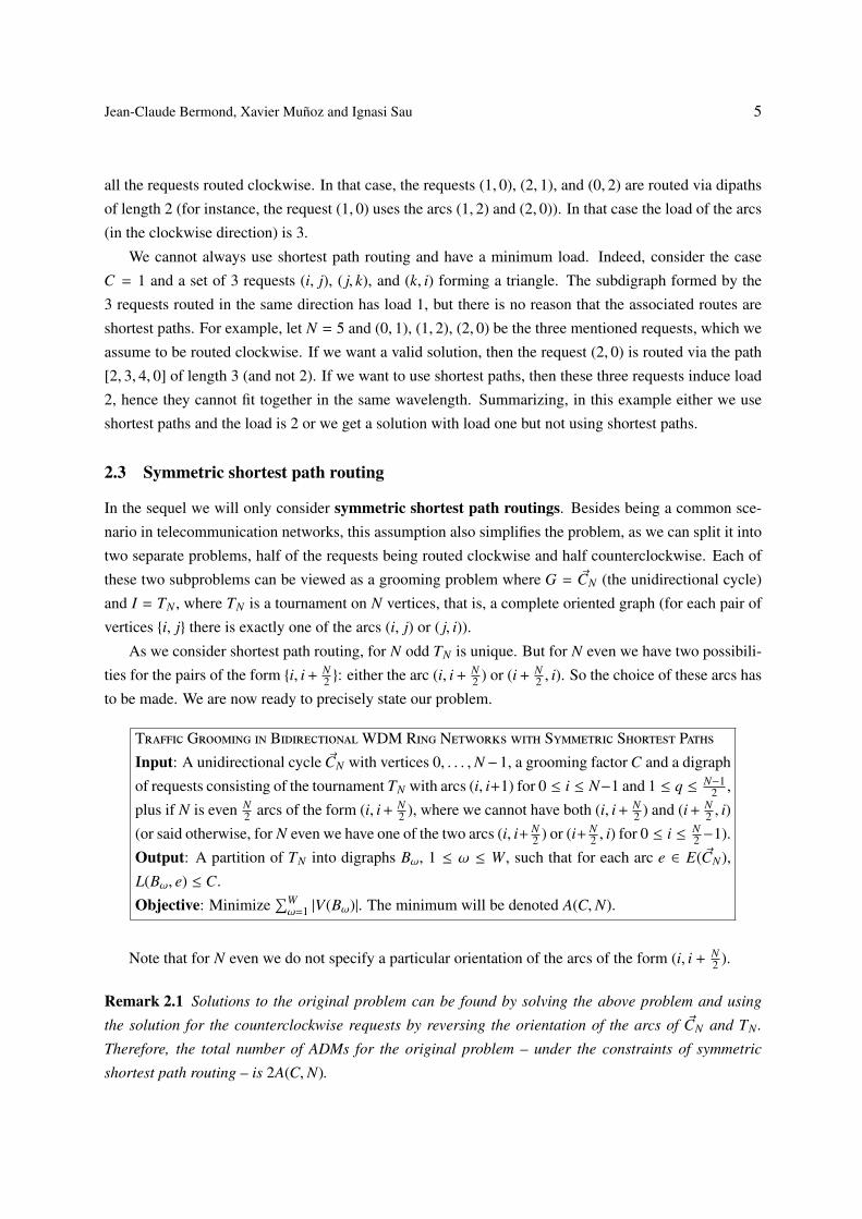
Traffic Grooming in BidirectionalWDM Ring Networks with Symmetric Shortest Paths
Input: A unidirectional cycle ~CN with vertices 0, . . . ,N −1, a grooming factor C and a digraph
of requests consisting of the tournament TN with arcs (i, i+1) for 0 ≤ i ≤ N−1 and 1 ≤ q ≤ N−12 ,
plus if N is even N2 arcs of the form (i, i + N
2 ), where we cannot have both (i, i + N2 ) and (i + N
2 , i)
(or said otherwise, for N even we have one of the two arcs (i, i+ N2 ) or (i+ N
2 , i) for 0 ≤ i ≤ N2 −1).
Output: A partition of TN into digraphs Bω, 1 ≤ ω ≤ W, such that for each arc e ∈ E( ~CN),
L(Bω, e) ≤ C.
Objective: Minimize∑Wω=1 |V(Bω)|. The minimum will be denoted A(C,N).
Note that for N even we do not specify a particular orientation of the arcs of the form (i, i + N2 ).
Remark 2.1 Solutions to the original problem can be found by solving the above problem and using
the solution for the counterclockwise requests by reversing the orientation of the arcs of ~CN and TN .
Therefore, the total number of ADMs for the original problem – under the constraints of symmetric
shortest path routing – is 2A(C,N).
6 Traffic grooming in bidirectional WDM ring networks
Let us see an example for N = 5 and C = 1. Then the following three subdigraphs form a solution
with 10 ADMs: one with arcs (0, 1), (1, 3), (3, 0), another with arcs (1, 2), (2, 4), (4, 1), and another with
arcs (0, 2), (2, 3), (3, 4), (4, 0). Thus, a solution for the bidirectional ring C∗5 and I = K∗5 needs 20 ADMs.
Let now N = 5 and C = 2. We can use the preceding solution or another one with also 10 ADMs
with only two ~C5’s with arcs (0, 2), (1, 2), (2, 3), (3, 4), (4, 5) and (0, 2), (2, 4), (4, 1), (1, 3), (3, 0), the sec-
ond one inducing load 2. But we can do better, with only 8 ADMs, with one subdigraph with arcs
(1, 3), (3, 4), (4, 1), and another one with arcs (0, 1), (1, 2), (0, 2), (2, 3), (2, 4), (3, 0), (4, 0). This latter par-
tition is optimal. In that case, we need 16 ADMs for the bidirectional ring.
To tackle our problem we will use tools from design theory, similar to those used for the unidirec-
tional ring and I = KN [7,8]. In particular, it is helpful to use, for a given C, digraphs having a maximum
ratio of the number of arcs to the number of vertices (see Section 3.2).
2.4 Admissible digraphs
Let Bω = (Vω, Eω) be a digraph with Vω = {a0, . . . , ap−1} involved in a partition of the tournament TN .
Note that the edges of Bω belong to TN , so (ai, a j) ∈ Eω if and only d ~CN(ai, a j) ≤ N
2 , where d ~CN(ai, a j) is
the distance between ai and a j in ~CN .
A digraph Bω is said to be admissible if it satisfies the load constraint, that is, L(Bω, e) ≤ C for each
arc e ∈ E( ~CN). A partition of TN into admissible subdigraphs is called valid. As the paths associated
with an arc of Bω form a dipath (an interval) in ~CN , the load is exactly the same as if we consider Bωembedded in a cycle ~Cp with vertex set 0, 1, . . . , p− 1. More precisely, we associate with Bω the digraph
Bpω having vertices 0, 1, . . . , p − 1 and with (i, j) ∈ E(Bp
ω) if and only if (ai, a j) ∈ E(Bω). Hence, to
compute the load we will consider digraphs with p vertices and their load in the associated ~Cp. Note that
it can happen that d ~CN(ai, a j) ≤ N
2 but d ~Cp(i, j) > p
2 , and vice versa.
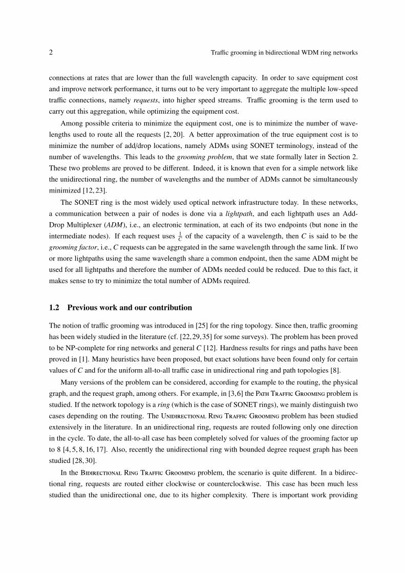
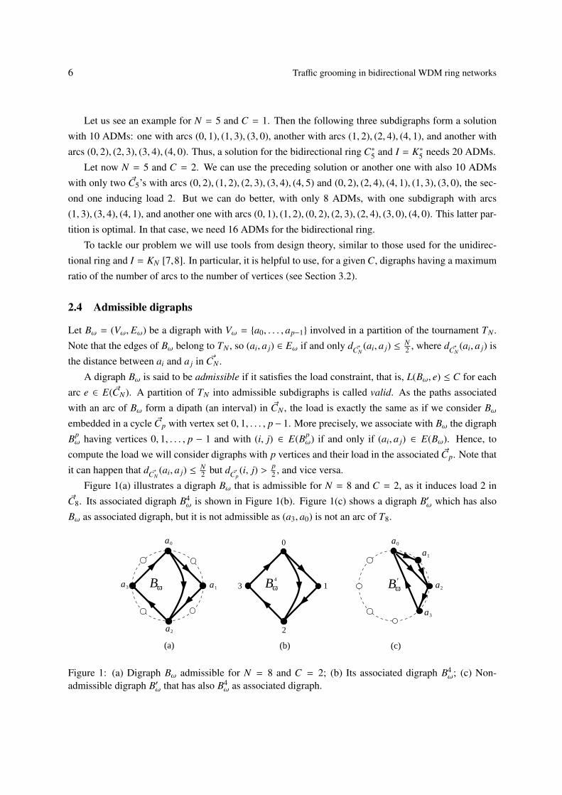
Figure 1(a) illustrates a digraph Bω that is admissible for N = 8 and C = 2, as it induces load 2 in~C8. Its associated digraph B4
ω is shown in Figure 1(b). Figure 1(c) shows a digraph B′ω which has also
Bω as associated digraph, but it is not admissible as (a3, a0) is not an arc of T8.
0
4
(b)
Bω3
2
1
a0
a1
a2
a3
(a)
Bω
a0
a1
a2
a3
(c)
Bω'
Figure 1: (a) Digraph Bω admissible for N = 8 and C = 2; (b) Its associated digraph B4ω; (c) Non-
admissible digraph B′ω that has also B4ω as associated digraph.
Jean-Claude Bermond, Xavier Munoz and Ignasi Sau 7
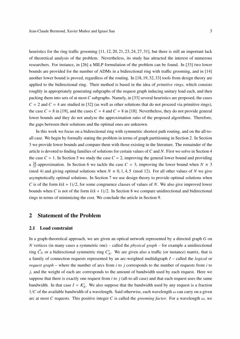
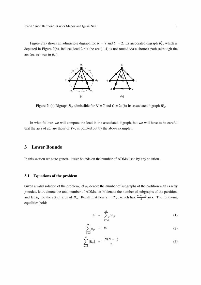
Figure 2(a) shows an admissible digraph for N = 7 and C = 2. Its associated digraph B5ω, which is
depicted in Figure 2(b), induces load 2 but the arc (1, 4) is not routed via a shortest path (although the
arc (a1, a4) was in Bω).
0a0
a1
a2
a4
(a)
Bω
a3
(b)
Bω5
1
23
4
Figure 2: (a) Digraph Bω admissible for N = 7 and C = 2; (b) Its associated digraph B5ω.
In what follows we will compute the load in the associated digraph, but we will have to be careful
that the arcs of Bω are those of TN , as pointed out by the above examples.
3 Lower Bounds
In this section we state general lower bounds on the number of ADMs used by any solution.
3.1 Equations of the problem
Given a valid solution of the problem, let ap denote the number of subgraphs of the partition with exactly
p nodes, let A denote the total number of ADMs, let W denote the number of subgraphs of the partition,
and let Eω be the set of arcs of Bω. Recall that here I = TN , which has N(N−1)2 arcs. The following
equalities hold:
A =
N∑p=2
pap (1)
N∑p=2
ap = W (2)
W∑w=1
|Eω| =N(N − 1)
2(3)

8 Traffic grooming in bidirectional WDM ring networks
Proposition 3.1 For I = TN ,
W ≥⌈
N2 + α
8C
⌉, where α =
−1, if N is odd
4, if N ≡ 2 (mod 4)
8, if N ≡ 0 (mod 4)
Proof: The set of arcs of TN of the form (i, i + q), 0 ≤ q < N2 , load each arc of the ring exactly q times.
So if N is odd the load of any arc of the ring is 1 + 2 + · · · + N−12 = N2−1
8 .
If N is even the load due to these arcs is 1 + 2 + · · · + N−22 = N2−2N
8 . We have to add the load due to
arcs of TN of the form(i, i + N
2
). As there are N
2 such arcs, the total load is N2
4 and so one arc of the ring
has load at least N4 .
If N ≡ 2 (mod 4) that gives a load at least⌈
N4
⌉= N+2
4 , so one arc has load at least N2−2N8 + N+2
4 = N2+48 .
If N ≡ 0 (mod 4) the maximum load due to the arcs(i, i + N
2
)is at least N
4 , but in this case we can
give a better bound. Indeed, suppose w.l.o.g. that we have the arc(0, N
2
), and let j be the number of arcs
starting in the interval [1, N2 − 1] of the form
(i, i + N
2
)with 0 < i < N
2 . The load of the arc(
N2 − 1, N
2
)of
the ring is then j + 1. As there are N2 − 1 − j arcs ending in the interval [1, N
2 − 1], the load of the arc(0, 1) is 1 + N
2 − 1 − j. Therefore the sum of the loads of the arcs (0, 1) and(
N2 − 1, N
2
)is N
2 + 1, and so
one of these 2 arcs has load⌈
N4 + 1
2
⌉= N
4 + 1. The total load of this arc is N2−2N8 + N
4 + 1 = N2+88 .
As each subgraph can load one arc at most C times, we obtain the lemma. 2
3.2 The parameter γ(C, p)
To obtain accurate lower bounds we need to bound the value of |Eω| for a digraph with |Vω| = p ver-
tices, satisfying the load constraint (admissible digraph). As we discussed in the preceding section, we
need only to consider the associated digraph embedded in ~Cp. To this end, we introduce the following
definitions.
Definition 3.1 Let γ(C, p) be the maximum number of arcs of a digraph H with p vertices such that
L(H, e) ≤ C, for every arc e of ~Cp.
Definition 3.2ρ(C) = max
p≥2
{γ(C, p)
p
}.
In [33] the authors define two parameters which coincide with the parameters γ(C, p) and ρ(C) intro-
duced above. In [33] the parameter ρ(C) is called maximal ADM efficiency, and its value is determined,
but no closed formula for γ(C, p) is given in [33]. Here we give again the value of ρ(C), using different
tools, and give the exact value of γ(C, p).
The next proposition shows that, in fact, the maximum number of requests we can groom is attained
by taking those of minimum length. It is worth mentioning that this property is not true if the physical
graph is a path, as shown with a counterexample in [3].

Jean-Claude Bermond, Xavier Munoz and Ignasi Sau 9
Proposition 3.2 Let C =k(k+1)
2 + r, with 0 ≤ r ≤ k. Then
γ(C, p) =
p(p−1)
2 , if p ≤ 2k + 1, or p = 2k + 2 and r ≥ k+22
kp + 2r − 1 , if p = 2k + 2 and 1 ≤ r < k+22
kp +⌊
rpk+1
⌋, otherwise
The graphs achieving γ(C, p) are either the tournament Tp if p is small (namely, if p ≤ 2k+1 or p = 2k+2
and r ≥ k+22 ), or subgraphs of a circulant digraph containing all the arcs of length 1, 2, . . . , k, plus some
arcs of length k + 1 if r > 0.
Proof: We distinguish three cases according to the value of p.
Case 1. If p is small, that is such that the tournament Tp loads each arc at most C times, then
γ(C, p) =p(p−1)
2 . Let us now see for which values of p this fact holds.
If p is odd, the load of Tp is p2−18 ≤ C. The inequality p2 − 1 ≤ 8C implies p2 − 1 ≤ 4k(k + 1) + 8r,
and is satisfied if p ≤ 2k + 1, as p2 − 1 ≤ 4k(k + 1).
If p is even, the load of Tp is p2
8 + 1+δ2 , where δ = 1 if p ≡ 0 (mod 4) (see proof of Proposition 3.1).
If p ≤ 2k, then p2+88 ≤ 4k2+8
8 ≤k(k+1)
2 ≤ C.
For p = 2k + 2, then p2
8 + 1+δ2 = k2
2 + k + 1 + δ2 ≤
k2+k2 + r = C if and only if r ≥ k+2+δ
2 , with δ = 1 if
p ≡ 0 (mod 4), that is, if k is odd. Therefore, the condition is satisfied if r ≥ k+22 .
In the next two cases, we provide first a lower bound on γ(C, p), and then we prove a matching upper
bound.
Case 2. If p = 2k + 2 and 1 ≤ r < k+22 , a solution is obtained by taking all the arcs of length
1, 2, . . . , k(=
p−22
)– giving a load of k(k+1)
2 – plus 2r − 1 arcs of length p2 . For example, we can take the
arcs(i, i +
p2
)for i = 0, 2, . . . , 2r − 2
(<
p2
)and the arcs
(i, i − p
2
)for i = 1, 3, . . . , 2r − 3. The load due to
these arcs is at most r. Therefore, in this case γ(C, p) ≥ kp + 2r − 1.
Case 3. If p > 2k + 2 or p = 2k + 2 and r = 0, a solution is obtained by taking all the arcs of
length 1, 2, . . . , k plus⌊
rpk+1
⌋arcs of length k + 1, in such a way that the load due to these arcs is at
most C, which is always possible (for example, if p and k + 1 are relatively prime, we take the requests
((k + 1)i, (k + 1)(i + 1)) for 0 ≤ i ≤⌊
rpk+1
⌋− 1, the indices being taken modulo p). Therefore, in this case
γ(C, p) ≥ kp +
⌊ rpk + 1
⌋. (4)
Let us now turn to upper bounds. Suppose we have a solution with γ arcs, γi being of length i on ~Cp.
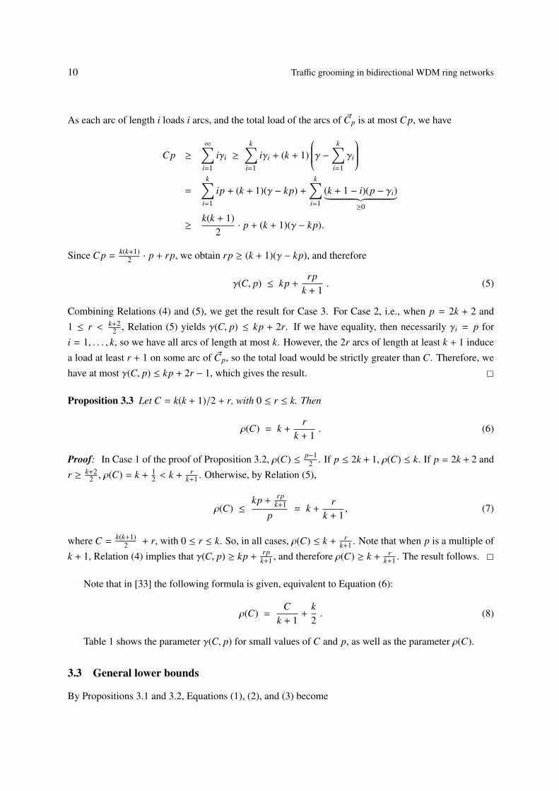
10 Traffic grooming in bidirectional WDM ring networks
As each arc of length i loads i arcs, and the total load of the arcs of ~Cp is at most Cp, we have
Cp ≥
∞∑i=1
iγi ≥
k∑i=1
iγi + (k + 1)
γ − k∑i=1
γi
=
k∑i=1
ip + (k + 1)(γ − kp) +
k∑i=1
(k + 1 − i)(p − γi)︸ ︷︷ ︸≥0
≥k(k + 1)
2· p + (k + 1)(γ − kp).
Since Cp =k(k+1)
2 · p + rp, we obtain rp ≥ (k + 1)(γ − kp), and therefore
γ(C, p) ≤ kp +rp
k + 1. (5)
Combining Relations (4) and (5), we get the result for Case 3. For Case 2, i.e., when p = 2k + 2 and
1 ≤ r < k+22 , Relation (5) yields γ(C, p) ≤ kp + 2r. If we have equality, then necessarily γi = p for
i = 1, . . . , k, so we have all arcs of length at most k. However, the 2r arcs of length at least k + 1 induce
a load at least r + 1 on some arc of ~Cp, so the total load would be strictly greater than C. Therefore, we
have at most γ(C, p) ≤ kp + 2r − 1, which gives the result. 2
Proposition 3.3 Let C = k(k + 1)/2 + r, with 0 ≤ r ≤ k. Then
ρ(C) = k +r
k + 1. (6)
Proof: In Case 1 of the proof of Proposition 3.2, ρ(C) ≤ p−12 . If p ≤ 2k + 1, ρ(C) ≤ k. If p = 2k + 2 and
r ≥ k+22 , ρ(C) = k + 1
2 < k + rk+1 . Otherwise, by Relation (5),
ρ(C) ≤kp +
rpk+1
p= k +
rk + 1
, (7)
where C =k(k+1)
2 + r, with 0 ≤ r ≤ k. So, in all cases, ρ(C) ≤ k + rk+1 . Note that when p is a multiple of
k + 1, Relation (4) implies that γ(C, p) ≥ kp +rp
k+1 , and therefore ρ(C) ≥ k + rk+1 . The result follows. 2
Note that in [33] the following formula is given, equivalent to Equation (6):
ρ(C) =C
k + 1+
k2. (8)
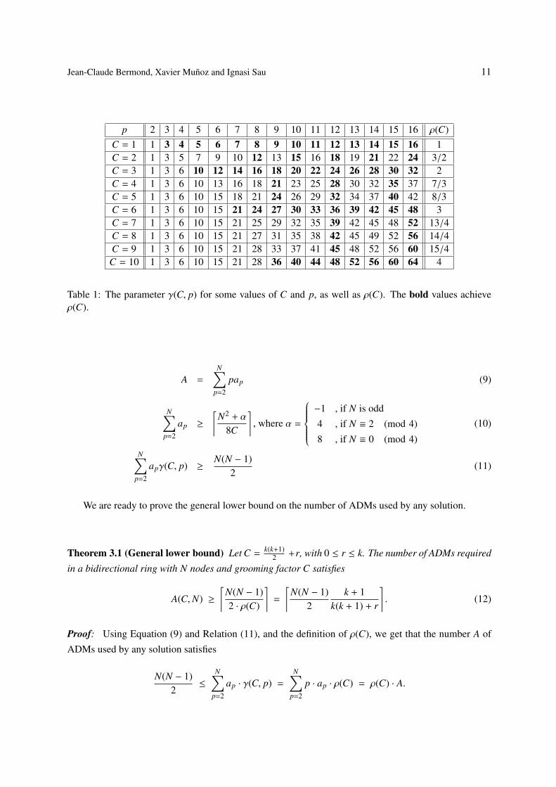
Table 1 shows the parameter γ(C, p) for small values of C and p, as well as the parameter ρ(C).
3.3 General lower bounds
By Propositions 3.1 and 3.2, Equations (1), (2), and (3) become
Jean-Claude Bermond, Xavier Munoz and Ignasi Sau 11
p 2 3 4 5 6 7 8 9 10 11 12 13 14 15 16 ρ(C)C = 1 1 3 4 5 6 7 8 9 10 11 12 13 14 15 16 1C = 2 1 3 5 7 9 10 12 13 15 16 18 19 21 22 24 3/2C = 3 1 3 6 10 12 14 16 18 20 22 24 26 28 30 32 2C = 4 1 3 6 10 13 16 18 21 23 25 28 30 32 35 37 7/3C = 5 1 3 6 10 15 18 21 24 26 29 32 34 37 40 42 8/3C = 6 1 3 6 10 15 21 24 27 30 33 36 39 42 45 48 3C = 7 1 3 6 10 15 21 25 29 32 35 39 42 45 48 52 13/4C = 8 1 3 6 10 15 21 27 31 35 38 42 45 49 52 56 14/4C = 9 1 3 6 10 15 21 28 33 37 41 45 48 52 56 60 15/4C = 10 1 3 6 10 15 21 28 36 40 44 48 52 56 60 64 4
Table 1: The parameter γ(C, p) for some values of C and p, as well as ρ(C). The bold values achieveρ(C).
A =
N∑p=2
pap (9)
N∑p=2
ap ≥
⌈N2 + α
8C
⌉, where α =
−1 , if N is odd
4 , if N ≡ 2 (mod 4)
8 , if N ≡ 0 (mod 4)
(10)
N∑p=2
apγ(C, p) ≥N(N − 1)
2(11)
We are ready to prove the general lower bound on the number of ADMs used by any solution.
Theorem 3.1 (General lower bound) Let C =k(k+1)
2 +r, with 0 ≤ r ≤ k. The number of ADMs required
in a bidirectional ring with N nodes and grooming factor C satisfies
A(C,N) ≥⌈
N(N − 1)2 · ρ(C)
⌉=
⌈N(N − 1)
2k + 1
k(k + 1) + r
⌉. (12)
Proof: Using Equation (9) and Relation (11), and the definition of ρ(C), we get that the number A of
ADMs used by any solution satisfies
N(N − 1)2
≤
N∑p=2
ap · γ(C, p) =
N∑p=2
p · ap · ρ(C) = ρ(C) · A.
12 Traffic grooming in bidirectional WDM ring networks
From the above relation and using Relation (7), we get
A ≥⌈
N(N − 1)2 · ρ(C)
⌉=
⌈N(N − 1)
2k + 1
k(k + 1) + r
⌉.
2
To achieve the lower bound of Theorem 3.1, the only possibility is to use graphs on p vertices with
γ(C, p) arcs. The bold values in Table 1 achieve ρ(C), and therefore the subgraphs corresponding to
those values (which exist by Proposition 3.2) are good candidates to construct an optimal partition of the
request graph.
Comparison with existing lower bounds. In [14] the Ring Traffic Grooming problem in the bidirec-
tional ring is studied. The authors state a lower bound regardless of routing for a general set of requests.
In the particular case of uniform traffic, they get a lower bound of N2−14√
2C(see [14, Theorem 1, page 198]).
They indicate in their article that they can improve this bound by a factor of 2 for all-to-all uniform
unitary traffic. We thank T. Chow and P. Lin for sending us the proof of the following theorem, which is
only announced in [14].
Theorem 3.2 ([13, 14]) If a traffic instance of ring grooming is uniform and unitary, then, regardless of
routing,
A(C,N) ≥1
2√
C
√N2(N − 1)2
2− N(N − 1).
The lower bound we obtained in Theorem 3.1 is greater than the bound of Theorem 3.2, but it should
be observed that we restrict ourselves to shortest path symmetric routing. Our bound is N(N−1)2ρ(C) and the
lower bound of Theorem 3.2 is less than N(N−1)2√
2C. The fact that our bound is better follows from the fact
that ρ(C) <√
2C. Indeed,
ρ2(C) ≤(k +
rk + 1
)2= k2 +
2krk + 1
+r2
(k + 1)2 < k2 + 2r + 1 < k2 + k + 2r = 2C.
4 Case C = 1
For C = 1, by Proposition 3.2 γ(1, p) = p if p ≥ 2. Furthermore, all the directed cycles achieve ρ(1) (see
Table 1).
Theorem 4.1
A(1,N) =
N(N−1)2 , if N is odd
N2
2 , if N is even
Jean-Claude Bermond, Xavier Munoz and Ignasi Sau 13
Proof: For C = 1, the only possible subgraphs involved in the partition of the edges of TN are cycles
and paths. If only cycles are used, the total number of ADMs is N(N−1)2 , which equals the lower bound of
Theorem 3.1. Each path involved in the partition adds one unit of cost with respect to N(N−1)2 .
If N = 2q + 1 is odd, by [10, Theorem 3.3] we know that the arcs of TN can be covered with q ~C3’s
and q(q−1)2
~C4’s. The total number of vertices of this construction is 3q + 2q(q − 1) = q(2q + 1) =N(N−1)
2 .
If N is even, each vertex must appear with odd degree in at least one subgraph, so the number
of paths in any construction is at least N/2. Therefore, the lower bound becomes N(N−1)2 + N
2 = N2
2 .
By [10, Theorem 3.4] the arcs of TN can be covered with
• 4 ~C3’s and 2q2 − 3 ~C4’s, if N = 4q with q > 1;
• 2 ~C3’s and 2q2 + 2q − 1 ~C4’s, if N = 4q + 2.
For N = 4, we cover T4 with a ~C4 and two arcs. Note that in these constructions, some arcs are covered
more than once. In both cases, the total number of vertices of the construction is N2
2 , hence the lower
bound is attained.
Finally, one can check that in the constructions of [10], the length of the arcs involved in the covering
of TN is in all cases bounded above by⌊
N2
⌋, and therefore all the cycles induce load 1. 2
Remark 4.1 For the original problem with G = C∗N and I = K∗N , if we apply Theorem 4.1 we get in the
case N even a value of N2 ADMS; but if we delete the constraint of symmetric routings we get a value of
N(N − 1)/2 by using [10, Theorems 4.1 and 4.2] (however these constructions use many K2’s).
5 Case C = 2
When C = 2 the general lower bound of Theorem 3.1 gives A(2,N) ≥ N(N−1)3 . We first improve this
bound in Section 5.1, and then give solutions with a good approximation ratio in Section 5.2.
5.1 Improved lower bounds
For C = 2, by Proposition 3.2 γ(2, 2) = 1, γ(2, 3) = 3, γ(2, 4) = 5 (note that γ(2, 4) = 6 if the routing
is not restricted to be symmetric), and γ(2, p) =⌊ 3p
2
⌋for p ≥ 5. The optimal solutions for p ≥ 4 even
consist of the p arcs of length 1 (i, i + 1) for 0 ≤ i ≤ p − 1, plus the p/2 arcs of length 2 (2i, 2i + 2) for
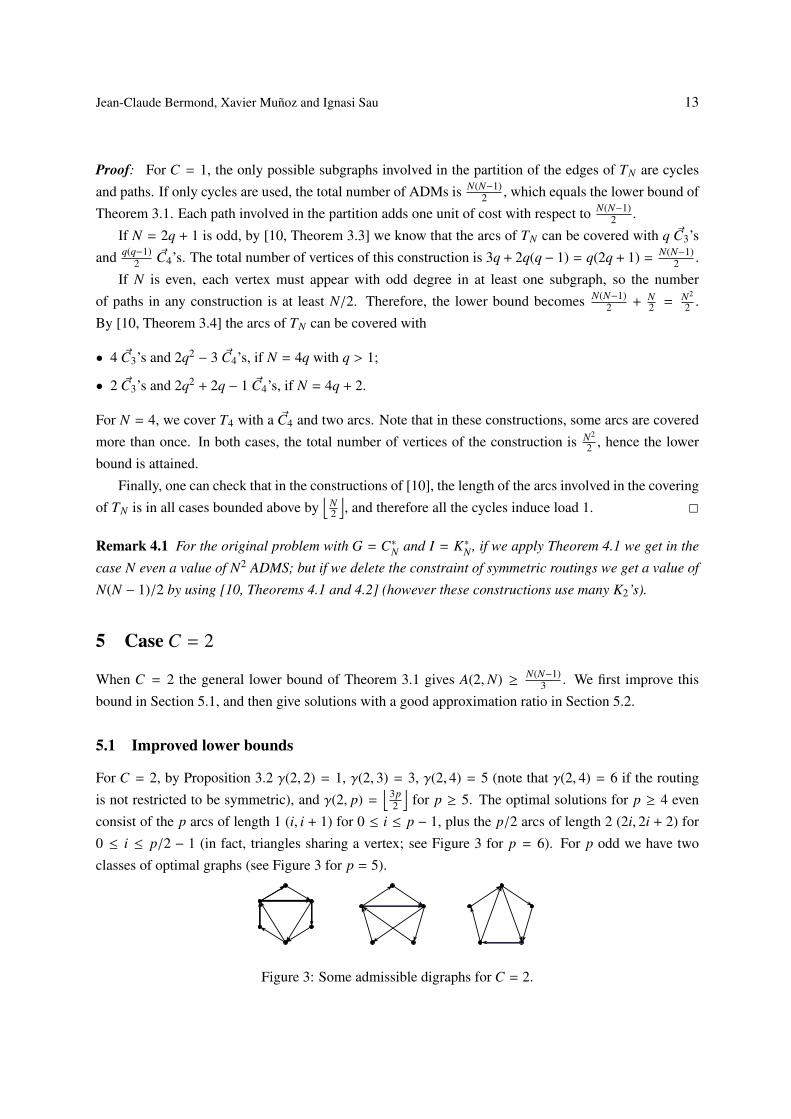
0 ≤ i ≤ p/2 − 1 (in fact, triangles sharing a vertex; see Figure 3 for p = 6). For p odd we have two
classes of optimal graphs (see Figure 3 for p = 5).
Figure 3: Some admissible digraphs for C = 2.
14 Traffic grooming in bidirectional WDM ring networks
Relation (11) becomes in the case C = 2
N∑p=2
apγ(2, p) = a2 + 3a3 + 5a4 + 7a5 + 9a6 + 10a7 + 12a8 + · · · ≥N(N − 1)
2.
Therefore,
A =
N∑p=2
pap ≥23
N∑p=2
apγ(2, p) +43
a2 + a3 +23
a4 +13
(a5 + a7 + a9 + · · · ) (13)
≥N(N − 1)
3+
43
a2 + a3 +23
a4 +13
(a5 + a7 + a9 + · · · ). (14)
We can already see that the bound N(N−1)3 cannot be attained. Indeed, to reach it we need to use only
graphs with 6, 8, 10, . . . vertices. But the number of graphs W satisfies, by Proposition 3.1, W ≥ N2−116 , so
A ≥ 6 N2−116 > N(N−1)
3 .
The following proposition gives a lower bound of order 1132 N(N−1). Note that 11/32 > 11/33 = 1/3.
Proposition 5.1 (Tighter lower bound for C = 2)
A(2,N) ≥⌈11N2 − 8N − 3
32
⌉=
⌈1116
N(N − 1)2
+3N − 3
32
⌉. (15)
Proof: We can write A ≥ 6(W − a2 − a3 − a4 − a5) + 2a2 + 3a3 + 4a4 + 5a5, that is,
A ≥ 6W − (4a2 + 3a3 + 2a4 + a5). (16)
From Relations (13) and (14) we get
3A ≥ N(N − 1) + (4a2 + 3a3 + 2a4 + a5). (17)
Summing Relations (16) and (17) gives
4A ≥ 6W + N(N − 1). (18)
By Proposition 3.1, we have that
W ≥N(N − 1)
16+
N + α
16. (19)
Combining Relations (18) and (19) and using α ≥ −1 yields
A ≥11N(N − 1)
32+
3N32
+3α32≥
11N2 − 8N − 332
.

Jean-Claude Bermond, Xavier Munoz and Ignasi Sau 15
2
5.2 Upper bounds
In this section we build families of solutions for C = 2. We conjecture that there exists a decomposition
using A vertices with ratio AN(N−1)
2of order 11
16 , which would be optimal by Proposition 5.1. For that, we
should find some (multipartite) graphs achieving this ratio. A candidate is K4,4,4, which has 48 edges.
Unfortunately, we have not been able to cover it with 33 vertices (which would achieve the optimal ratio)
but only with 34, giving a 34/33-approximation.
For the sake of the presentation, we first present a simple 12/11-approximation inspired from a
construction of [10].
5.2.1 A 12/11-approximation
This construction is defined recursively. Suppose we have a solution for N vertices using AN ADMs, with
N = 2p or N = 2p+1. Let the vertex set be labeled 0A < 1A < · · · < (p−1)A < 0B < 1B < · · · < (p−1)B,
plus ∞ is N is odd. For N + 2, we add two vertices xA and xB with the order xA < 0A < 1A < · · · <
(p − 1)A < xB < 0B < 1B < · · · < (p − 1)B < ∞. We use as subdigraphs those of the solution for N
plus the bp/2c digraphs on the 6 vertices xA, iA, (i + bp/2c)A, xB, iB, (i + bp/2c)B and the 8 arcs (xA, iA),
(xA, (i + bp/2c)A), (iA, xB), ((i + bp/2c)A, xB), (xB, iB), (xB, (i + bp/2cB), (iB, xA), ((i + bp/2c)B, xA), for
0 ≤ i ≤ bp/2c − 1.
If N = 2p with p even, there remains uncovered the arc (xA, xB).
If N = 2p + 1 with p even, there remain the 3 arcs (xA, xB), (xB,∞), and (∞, xA), which we cover
with the circuit (xA, xB,∞).
If N = 2p with p odd, there remain the 5 arcs (xA, (p−1)A), ((p−1)A, xB), (xB, (p−1)B), ((p−1)B, xA),
and (xA, xB), which we cover with a digraph on 4 vertices containing all of them.
Finally, if N = 2p + 1 with p odd, there remain the 7 arcs (xA, (p − 1)A), ((p − 1)A, xB), (xB, (p −
1)B), ((p−1)B, xA), (xA, xB), (xB,∞), and (∞, xA), which we cover with a digraph on 5 vertices containing
all of them.
One can check that, in all cases, the arcs (u, v) considered satisfy d ~Cn(u, v) ≤ N/2.
To compute the number of ADMs of this construction, we have the recurrence relations A4q+2 =
A4q + 6q + 2, A4q+4 = A4q+2 + 6q + 4, A4q+3 = A4q+1 + 6q + 3, and A4q+5 = A4q+3 + 6q + 5. Starting with
A2 = 2 or A4 = 6 (obtained with the partition with the digraph on 4 vertices formed by the C4 (0, 1, 2, 3)
plus the arc (0, 2) and the digraph on 2 vertices (1, 3)) and A3 = 3 or A5 = 8 (obtained with the partition
of T5 using the first digraph on 5 vertices of Figure 3 and the remaining T3), we get A4q = 6q2 = 6N2
16 ,
A4q+2 = 6q2 + 6q + 2 = 6N2+816 , A4q+1 = 6q2 + 2q = 6N2−4N−2
16 , and A4q+3 = 6q2 + 8q + 3 = 6N2−4N+616 .
In all cases, the number of ADMs is of order 68
N(N−1)2 , so asymptotically the ratio between the number
of ADMs of this construction and the lower bound of Proposition 5.1 tends to 68
1611 = 12
11 .

16 Traffic grooming in bidirectional WDM ring networks
5.2.2 A 34/33-approximation
It will be useful to use the notation G5 and G6 to refer to the digraphs depicted in Figure 4. The key idea of
this construction is that an oriented tripartite graph K4,4,4 can be partitioned into admissible subdigraphs
for C = 2 using 34 vertices overall, as follows.
Let the tripartition classes of the K4,4,4 be {1A, 1B, 1C , 1D}, {2A, 2B, 2C , 2D}, {3A, 3B, 3C , 3D}, and let
the vertices be ordered in the ring 1A < 2A < 3A < 1B < 2B < 3B < 1C < 2C < 3C < 1D <
2D < 3D. The arcs of an oriented K4,4,4 can be partitioned into 4 G6’s with {x1, x2, x3, x4, x5, x6} =
{1A, 2A, 3B, 1C , 2C , 3D}, {1B, 2B, 3B, 1D, 2D, 3D}, {1B, 2C , 3C , 1D, 2A, 3A}, and {1A, 3A, 2B, 1C , 3C , 2D}, plus
2 G5’s with {x1, x2, x3, x4, x5} = {3A, 1C , 2C , 1D, 2D} and {3D, 2A, 2B, 1D, 1C} (see Figure 4). The total
number of vertices of this partition is 34.
G6G5x1 x2
x2
x3
x3
x4
x4 x5
x5 x6
x1
G7
Figure 4: Digraphs G5 and G6 used in the 34/33-approximation for C = 2, and digraph G7 suitable forC = 3 referred to in the proof of Proposition 6.2.
We are now ready to explain the construction. We take an integer p ≡ 1 or 3 (mod 6), hence Kp can
be partitioned into triangles. We replace each vertex i of Kp with 4 vertices iA, iB, iC , iD, and order the
vertices 1A < · · · < pA < 1B < 2B < · · · < pB < 1C < · · · < pC < 1D < · · · < pD. To a triple {i, j, k}
corresponding to a triangle of Kp, with i < j < k, we associate the decomposition described above of
the K4,4,4 on vertices {`A, `B, `C , `D : ` = i, j, k}. In this way, Kp×4 can be partitioned into p(p−1)6 K4,4,4’s,
or equivalently into p(p−1)6 · 4 G6’s and p(p−1)
6 · 2 G5’s. Overall, we use 34p(p−1)6 vertices. Each of the
subdigraphs of this partition is admissible, as the distance in the ring between the endpoints of an arc is
strictly smaller than 2p.
To partition an oriented K4p, there remain only the K4’s induced inside each class of the Kp×4. As
A(2, 4) = 6, we use 6p vertices to cover all the K4’s.
Therefore, if p ≡ 1 or 3 (mod 6), an oriented K4p can be partitioned using 6p +34p(p−1)
6 =34p2+2p
6 =34N2+8N
96 vertices. To decompose K4p+1, we add a vertex ∞, and we partition the p K5’s using 8 vertices
for each one of them. Overall, we use 8p +34p(p−1)
6 =34p2+14p
6 = 34N2−12N−2496 vertices.
If p . 1 or 3 (mod 6), we introduce dummy vertices to get p′ ≡ 1 or 3 (mod 6), we do the construc-
tion described above, and then we remove the dummy edges and vertices. It is clear that these dummy
vertices add O(N) vertices to the construction, hence the coefficient of the term N2 remains the same.
Since 33N2−24N−996 is a lower bound by Proposition 5.1, we get the following result.
Proposition 5.2 The above construction approximates A(2,N) within a factor 34/33.
Jean-Claude Bermond, Xavier Munoz and Ignasi Sau 17
6 Case C = 3
We first provide improved lower bounds for some congruence classes in Section 6.1 and then we provide
constructions in Section 6.2, which are either optimal or asymptotically optimal.
6.1 Improved lower bounds
In this case (see Table 1) we have γ(3, 2) = 1, γ(3, 3) = 3, γ(3, 4) = 6, and γ(3, p) = 2p for p ≥ 5, so
ρ(3) = 2. Therefore, by Theorem 3.1, we get
Proposition 6.1 A(3,N) ≥ N(N−1)4 .
By Relations (9) and (11) we have
2A =
N∑p=2
2pap = 4a2 + 6a3 + 8a4 +
N∑p=5
2pap
N(N − 1)2
≤
N∑p=2
apγ(3, p) = a2 + 3a3 + 6a4 +
N∑p=5
2pap
So
A ≥N(N − 1)
4+
32
a2 +32
a3 + a4.
Therefore, if the lower bound is attained, then necessarily a2 = a3 = a4 = 0. We will see in Section 6.2
that this is the case for N ≡ 1 or 5 (mod 12), using optimal digraphs on 5 vertices (namely T5) and on 6
vertices (namely ~K2,2,2, see Figure 5). Optimal graphs are obtained by using arcs of length 1 and 2, so the
degree of any vertex in an optimal subdigraph is 4. That is possible only if the total degree of a vertex,
namely N − 1, is a multiple of 4. Otherwise, the following proposition shows that the lower bound of
Proposition 6.1 cannot be attained.
Proposition 6.2 mh
If N ≡ 3 (mod 4), A(3,N) ≥ N(N−1)4 + N
6 = 3N2−N12 .
If N ≡ 0 (mod 2), A(3,N) ≥ N(N−1)4 + N
4 = N2
4 .
Proof: We use the following observation: If a vertex x has out-degree 3 (resp. in-degree 3) in a digraph
Bω, then its nearest out-neighbor A+x (resp. in-neighbor A−x ) has in-degree 1 and out-degree at most 1
(resp. out-degree 1 and in-degree at most 1). Indeed, suppose x has out-degree 3, and let A+x , B
+x ,C
+x be
the out-neighbors of x. Then the load of the arc entering A+x is already 3, so A+
x has no other in-neighbor
than x. The load of the arc leaving A+x is already 2, so A+
x has at most 1 out-neighbor y. If y has 2 or more
in-neighbors, then A+x is not its nearest one. Hence, to each vertex x of out-degree 3 (resp. in-degree 3)
is associated a distinct vertex A+x (resp. A−x ) of degree at most 2.
18 Traffic grooming in bidirectional WDM ring networks
Consider the digraphs in which a given vertex x appears. Let αxi be the number of times x appears
with degree i, and let αi =∑
x αxi . Vertex x appears in
∑i α
xi digraphs, so
A =∑
x
∑i
αxi =
∑i
αi. (20)
As each vertex has degree N − 1, N − 1 =∑
i i · αxi , and so
N(N − 1) =∑
x
∑i
i · αxi =
∑i
i · αi. (21)
Due to the load constraint, a vertex has out-degree (resp. in-degree) at most 3 in all the digraphs in
which it appears. Therefore, its degree is at most 6, that is, αi = 0 for i ≥ 7. Furthermore, by the above
observation if a vertex has degree 6 (resp. 5), to this vertex are associated 2 vertices (resp. 1 vertex) of
degree at most 2, and all these vertices are distinct, so
α1 + α2 ≥ 2α6 + α5. (22)
Combining Equations (20) and (21) we get
4A = N(N − 1) + 3α1 + 2α2 + α3 − α5 − 2α6. (23)
We distinguish two cases: N even or N = 4t + 3.
If N is even, N − 1 is odd and each vertex must appear at least in one Bω with odd degree, so
α1 + α3 + α5 ≥ N. (24)
Using Relation (22) multiplied by 2 in Relation (23) we get 4A ≥ N(N − 1) + α1 + α3 + α5 + 2α6, so by
Relation (24), 4A ≥ N(N−1)+ N, as claimed. Note that to obtain equality we need α6 = 0, α1 +α2 = α5,
and α1 + α3 + α5 = N.
If N = 4t + 3, the degree of each vertex satisfies N − 1 ≡ 2 (mod 4), so no vertex can appear with
degree 4 in all the digraphs. Each vertex must appear either at least once with degree 6 or 2, or at least
twice with odd degree (for example, 5 and 5, 3 and 3, 1 and 1, or 5 and 1), so
α2 + α6 +12
(α1 + α3 + α5) ≥ N. (25)
Equation (23) can be rewritten as
4A = N(N − 1) +23
(α2 + α6 +
12
(α1 + α3 + α5))
+43
(α2 + α1 − 2α6 − α5) +23α3 +
43α1. (26)
Using Relations (22) and (25) in Relation (26) yields 4A ≥ N(N−1)+ 23 N + 2
3α3 + 43α1, or A ≥ N(N−1)
4 + N6 ,
Jean-Claude Bermond, Xavier Munoz and Ignasi Sau 19
as claimed. Note that to reach the equality, we need to have α1 = α3 = 0, α2 = 2α6 +α5 by Relation (22),
and 2α6 + 2α2 + α5 = 2N by Relation (25), so α2 = 2N3 , hence an optimal decomposition should use N
3
digraphs like the digraph G7 depicted in Figure 4, having 1 vertex of degree 6 and 2 vertices of degree 2.
2
6.2 Constructions
Our constructions rely on the existence of 3-GDD’s, that is, decompositions of complete multipartite
graphs into K3’s. We recall the definition and some basic results below.
Decompositions of complete multipartite graphs into K3’s. Let v1, v2, . . . , vq be non-negative inte-
gers; the complete multipartite graph with group sizes v1, v2, . . . , vq is defined to be the graph with vertex
set V1 ∪ V2 ∪ · · · ∪ Vq where |Vi| = vi, and two vertices u ∈ Vi and v ∈ V j are adjacent if i , j. Using
terminology of design theory, the graph of type pα11 pα2
2 . . . pαhh is the complete multipartite graph with
αi groups of size pi. The existence of a partition of this multipartite graph into Kk’s is equivalent to the
existence of a k-GDD (Group Divisible Design) of type pα11 pα2
2 . . . pαhh (see [15]). Here we are interested
in the existence of 3-GDD’s, that is, partitions into K3’s. When |Vi| = p for all i, we denote by Kp×q the
multipartite graph of type pq. Trivial necessary conditions for the existence of a 3-GDD are
(i) the degree of each vertex is even; and(ii) the number of edges is a multiple of 3.
These conditions are in general sufficient. In particular, the following results will be used later.
Theorem 6.1 ([15]) espai.
A 3-GDD of type 2q with q ≥ 3 exists if and only if q ≡ 0 or 1 (mod 3).
A 3-GDD of type 2q−14 with q ≥ 4 exists if and only if q ≡ 1 (mod 3).
A 3-GDD of type 3q with q ≥ 3 exists if and only if q is odd.
A 3-GDD of type 3q−11 with q ≥ 3 exists if and only if q is odd.
A 3-GDD of type 3q−15 with q ≥ 5 exists if and only if q is odd.
A 3-GDD of type 3q−111 with q ≥ 7 exists if and only if q is odd.
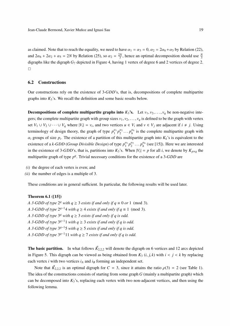
The basic partition. In what follows ~K2,2,2 will denote the digraph on 6 vertices and 12 arcs depicted
in Figure 5. This digraph can be viewed as being obtained from K3 (i, j, k) with i < j < k by replacing
each vertex i with two vertices iA and iB forming an independent set.
Note that ~K2,2,2 is an optimal digraph for C = 3, since it attains the ratio ρ(3) = 2 (see Table 1).
The idea of the constructions consists of starting from some graph G (mainly a multipartite graph) which
can be decomposed into K3’s, replacing each vertex with two non-adjacent vertices, and then using the
following lemma.
20 Traffic grooming in bidirectional WDM ring networks
K2,2,2iA
i
jk
jA
kA
iBjB
kB
(a)
T5
iA
ji jAiB
jB
(b)
8
8
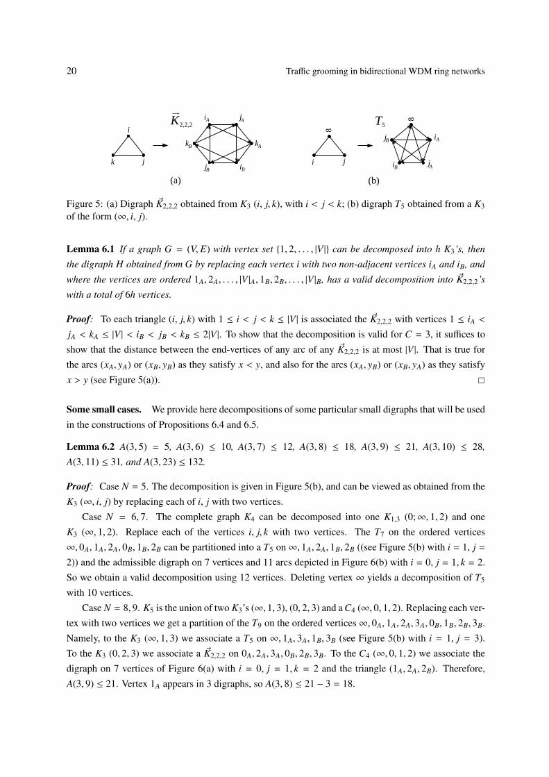
Figure 5: (a) Digraph ~K2,2,2 obtained from K3 (i, j, k), with i < j < k; (b) digraph T5 obtained from a K3of the form (∞, i, j).
Lemma 6.1 If a graph G = (V, E) with vertex set {1, 2, . . . , |V |} can be decomposed into h K3’s, then
the digraph H obtained from G by replacing each vertex i with two non-adjacent vertices iA and iB, and
where the vertices are ordered 1A, 2A, . . . , |V |A, 1B, 2B, . . . , |V |B, has a valid decomposition into ~K2,2,2’s
with a total of 6h vertices.
Proof: To each triangle (i, j, k) with 1 ≤ i < j < k ≤ |V | is associated the ~K2,2,2 with vertices 1 ≤ iA <
jA < kA ≤ |V | < iB < jB < kB ≤ 2|V |. To show that the decomposition is valid for C = 3, it suffices to
show that the distance between the end-vertices of any arc of any ~K2,2,2 is at most |V |. That is true for
the arcs (xA, yA) or (xB, yB) as they satisfy x < y, and also for the arcs (xA, yB) or (xB, yA) as they satisfy
x > y (see Figure 5(a)). 2
Some small cases. We provide here decompositions of some particular small digraphs that will be used
in the constructions of Propositions 6.4 and 6.5.
Lemma 6.2 A(3, 5) = 5, A(3, 6) ≤ 10, A(3, 7) ≤ 12, A(3, 8) ≤ 18, A(3, 9) ≤ 21, A(3, 10) ≤ 28,
A(3, 11) ≤ 31, and A(3, 23) ≤ 132.
Proof: Case N = 5. The decomposition is given in Figure 5(b), and can be viewed as obtained from the
K3 (∞, i, j) by replacing each of i, j with two vertices.
Case N = 6, 7. The complete graph K4 can be decomposed into one K1,3 (0;∞, 1, 2) and one
K3 (∞, 1, 2). Replace each of the vertices i, j, k with two vertices. The T7 on the ordered vertices
∞, 0A, 1A, 2A, 0B, 1B, 2B can be partitioned into a T5 on∞, 1A, 2A, 1B, 2B ((see Figure 5(b) with i = 1, j =
2)) and the admissible digraph on 7 vertices and 11 arcs depicted in Figure 6(b) with i = 0, j = 1, k = 2.
So we obtain a valid decomposition using 12 vertices. Deleting vertex ∞ yields a decomposition of T5
with 10 vertices.
Case N = 8, 9. K5 is the union of two K3’s (∞, 1, 3), (0, 2, 3) and a C4 (∞, 0, 1, 2). Replacing each ver-
tex with two vertices we get a partition of the T9 on the ordered vertices∞, 0A, 1A, 2A, 3A, 0B, 1B, 2B, 3B.
Namely, to the K3 (∞, 1, 3) we associate a T5 on ∞, 1A, 3A, 1B, 3B (see Figure 5(b) with i = 1, j = 3).
To the K3 (0, 2, 3) we associate a ~K2,2,2 on 0A, 2A, 3A, 0B, 2B, 3B. To the C4 (∞, 0, 1, 2) we associate the
digraph on 7 vertices of Figure 6(a) with i = 0, j = 1, k = 2 and the triangle (1A, 2A, 2B). Therefore,
A(3, 9) ≤ 21. Vertex 1A appears in 3 digraphs, so A(3, 8) ≤ 21 − 3 = 18.

Jean-Claude Bermond, Xavier Munoz and Ignasi Sau 21
i
j
k
A
B
A
A
i
j
k
B
B
lA
lB
(c)
j
k
B
A
A
i
j
k
B
B
8
iA
(b)
i
j
k
AB
A
A
i
j
k
B
B
8
(a)
Figure 6: (a) Digraph associated to a C4 (∞, i, j, k). Digraphs associated to stars (K1,3’s), with ∞ < i <j < k < `: (b) star of the form (i;∞, j, k); (c) star of the form (i; j, k, `).
Case N = 10, 11. K6 can be partitioned into 3 K3’s (∞, 1, 3), (∞, 2, 4), (0, 1, 4), a star K1,3 (0;∞, 2, 3),
and a P4 [1, 2, 3, 4]. Replacing each vertex with two vertices we get a partition of the T11 on the ordered
vertices ∞, 0A, 1A, 2A, 3A, 4A, 0B, 1B, 2B, 3B, 4B into 2 T5’s on ∞, 1A, 3A, 1B, 3B and ∞, 2A, 4A, 2B, 4B, a~K2,2,2 on 0A, 1A, 4A, 0B, 1B, 4B, a digraph on 7 vertices and 11 arcs depicted in Figure 6(b) with i = 0, j =
2, k = 3, and an admissible digraph on 8 vertices with arcs (1A, 2A), (2A, 3A), (3A, 4A), (1B, 2B), (2B, 3B), (3B, 4B),
(2A, 1B), (2B, 1A), (3A, 2B), (3B, 2A), (4A, 3B), (4B, 3A). Therefore, A(3, 11) ≤ 31, and as vertex ∞ appears
in 3 subgraphs, we get A(3, 10) ≤ 28.
Case N = 23. We decompose K12 into 19 K3’s and 3 K1,3’s, where vertex ∞ appears in 5 K3’s and
in a star (i;∞, j, k), the two other stars being of the form (i′; j′k′, `′) with i′ < j′ < k′ < `′. We obtain
a decomposition of T23 into 5 T5’s, 14 ~K2,2,2’s, 1 digraph of Figure 6(a), and 2 digraphs of Figure 6(c).
Thus, A(3, 23) ≤ 5 · 5 + 14 · 6 + 7 + 8 + 8 = 132. 2
Constructions. We begin with an optimal partition for N ≡ 0, 1, 4, or 5 (mod 12), and then we provide
near-optimal constructions for the remaining values.
Proposition 6.3 mh
If N ≡ 0 or 4 (mod 12), A(3,N) = N2
4 .
If N ≡ 1 or 5 (mod 12), A(3,N) =N(N−1)
4 .
Proof: The lower bound follows from Propositions 6.1 and 6.2. For the upper bound, we will apply
Lemma 6.1 with G = K2×q (type 2q), which can be decomposed by Theorem 6.1 into 2q(q−1)3 K3’s if
q ≡ 0 or 1 (mod 3). As G has 2q vertices, the graph H described in Lemma 6.1 has 4q vertices and can be
decomposed into admissible ~K2,2,2’s. Adding an admissible T4 on each of the q independent sets of H (of
the form {iA, jA, iB, jB} where {i, j} is an independent set of G), we get a valid decomposition of T4q into
q T4’s and 2q(q−1)3 admissible ~K2,2,2’s. So using A(3, 4) = 4, we get A(3, 4q) ≤ qA(3, 4) + 4q(q − 1) = 4q2
for q ≡ 0 or 1 (mod 3). So A(3,N) ≤ N2
4 for N ≡ 0 or 4 (mod 12).
For N = 4q + 1, we add to the vertex set of H an extra vertex ∞. Adding to the arcs of H the q
tournaments T5 built on∞, iA, jA, iB, jB, where vertices i, j are not adjacent in G, we get a decomposition
22 Traffic grooming in bidirectional WDM ring networks
of T4q+1 into q admissible T5’s plus 2q(q−1)3 admissible ~K2,2,2’s (the distance being at most 2q − 1 in H
and so 2q in T4q+1). Using A(3, 5) = 5 (see Lemma 6.2), we get A(3, 4q + 1) ≤ qA(3, 5) + 4q(q − 1) =
4q2 + q =(4q+1)4q
4 for q ≡ 0 or 1 (mod 3). So A(3,N) ≤ N(N−1)4 for N ≡ 1 or 5 (mod 12). 2
We group the non-optimal constructions in Proposition 6.4 and Proposition 6.5 according to whether
they differ from the lower bound by either a constant or a linear additive term, respectively.
Proposition 6.4 mh
If N ≡ 8 (mod 12), A(3,N) ≤ N2
4 + 2.
If N ≡ 9 (mod 12), A(3,N) =N(N−1)
4 + 3.
Proof: We start from G of type 2q−14 with q ≡ 1 (mod 3), which can be decomposed by Lemma 6.1
into 2(q−1)(q+2)3 K3’s. As in the proof of Proposition 6.3, we get a decomposition of T4q+4 into q − 1 T4’s,
one T8 and 2(q−1)(q+2)3
~K2,2,2’s (indeed, the independent set Vq of G has 4 vertices, so in H it induces
an independent set of 8 vertices). So using A(3, 4) = 4 and A(3, 8) ≤ 18 (see Lemma 6.2), we get
A(3, 4q + 4) ≤ (q − 1)A(3, 4) + A(3, 8) + 4(q − 1)(q + 2) ≤ 4q2 + 8q + 6 =(4q+4)2
4 + 2 for q ≡ 1 (mod 3),
so A(3,N) ≤ N2
4 + 2 for N ≡ 8 (mod 12).
Similarly, adding a vertex ∞ to H we get a decomposition of T4q+1 into q − 1 T5’s, one T9 and
h =2(q−1)(q+2)
3 K3’s. So using A(3, 5) = 5 and A(3, 9) ≤ 21 we get A(3, 4q+5) ≤ (q−1)A(3, 5)+ A(3, 9)+
4(q − 1)(q + 2) ≤ 4q2 + 9q + 8 =(4q+5)(4q+4)
4 + 3 for q ≡ 1 (mod 3), so A(3,N) ≤ N(N−1)4 + 3 for N ≡ 9
(mod 12). 2
Proposition 6.5 mh
If N ≡ 2 (mod 12), A(3,N) ≤ N2
4 + N+46 .
If N ≡ 3 (mod 12), A(3,N) ≤ N2+34 .
If N ≡ 6 (mod 12), A(3,N) ≤ N2
4 + N6 .
If N ≡ 7 (mod 12), A(3,N) ≤ N2−14 .
If N ≡ 10 (mod 12), A(3,N) ≤ N2
4 + N+86 .
If N ≡ 11 (mod 12), A(3,N) ≤ N2+34 + ε, with ε = 1 for N = 11, 35.
Proof: We use as graph G of Lemma 6.1 a multipartite graph of type 3q−1u with 3(q− 1) + u vertices, in
order to get a decomposition of T6(q−1)+2u (resp. T6(q−1)+2u+1) into q − 1 T6’s (resp. T7’s), one T2u (resp.
T2u+1) and the digraph H itself decomposed by Lemma 6.1 into h =9(q−1)(q−2)
6 + u(q − 1) ~K2,2,2’s. We
distinguish several cases according to the value of u.
Case 1: u = 1, q ≥ 3 odd.
Let N ≡ 2 (mod 12), N = 6q − 4. Using A(3, 2) = 2 and A(3, 6) ≤ 10 we get A(3, 6q − 4) ≤
(q − 1)A(3, 6) + A(3, 2) + (q − 1)(9q − 12) ≤ 9q2 − 11q + 4 =(6q−4)2
4 + q = N2
4 + N+46 .
Let N ≡ 3 (mod 12), N = 6q − 3. Using A(3, 3) = 3 and A(3, 7) ≤ 12 we get A(3, 6q − 3) ≤
(q − 1)A(3, 7) + A(3, 3) + (q − 1)(9q − 12) ≤ 9q2 − 9q + 3 =(6q−3)2
4 + 34 = N2+3
4 .
Case 2: u = 3, q ≥ 3 odd.

Jean-Claude Bermond, Xavier Munoz and Ignasi Sau 23
Let N ≡ 6 (mod 12), N = 6q. Using A(3, 6) ≤ 10 we get A(3, 6q) ≤ qA(3, 6) + 9q(q− 1) ≤ 9q2 + q =N2
4 + N6 .
Let N ≡ 7 (mod 12), N = 6q + 1. Using A(3, 7) ≤ 12 we get A(3, 6q + 1) ≤ qA(3, 7) + 9q(q − 1) ≤
9q2 + 3q = N2−14 .
Case 3: u = 5, q ≥ 5 odd.
Let N ≡ 10 (mod 12), N = 6q + 4. Using A(3, 6) ≤ 10 and A(3, 10) ≤ 28 we get A(3, 6q + 4) ≤
(q − 1)A(3, 6) + A(3, 10) + (q − 1)(9q + 12) ≤ 9q2 + 13q + 6 =(6q+4)2
4 +6q+12
6 = N2
4 + N+86 .
Let N ≡ 11 (mod 12), N = 6q + 5. Using A(3, 7) ≤ 12 and A(3, 11) ≤ 31 we get A(3, 6q + 5) ≤
(q − 1)A(3, 7) + A(3, 11) + (q − 1)(9q + 12) ≤ 9q2 + 15q + 7 = N2+34 .
For q = 23 we have A(3, 23) ≤ 132 = 232−14 , one less than the value given by the preceding
construction. Using u = 11, q ≥ 7 odd, N = 6q + 17, A(3, 7) ≤ 12, and A(3, 23) ≤ 132 we get
A(3, 6q + 17) ≤ (q − 1)A(3, 7) + A(3, 23) + (q − 1)(9q + 48) ≤ 9q2 + 51q + 72 =(6q+17)2−1
4 = N2−14 . It
might be that A(3, 11) ≤ 30, and then the bound N2−14 would be also attained for N = 11 and 35. 2
7 Case C > 3
For C > 3, we distinguish two cases according to whether C is of the form k(k+1)2 or not. We focus on
those cases in Sections 7.1 and 7.2.
7.1 C not of the form k(k + 1)/2
If C is not of the form k(k+1)2 , we can improve the lower bound of Theorem 3.1, as we did for C = 2
in Proposition 5.1. We provide the details for C = 4 and sketch the ideas for C = 5, that show how to
improve the lower bound for any value of C not of the form k(k + 1)/2.
Proposition 7.1
A(4,N) ≥7
32N(N − 1) =
(314
+1
224
)N(N − 1).
Proof: The values of γ(4, p) are given in Table 1, so Relation (13) becomes in the case C = 4
A =
N∑p=2
pap ≥37
N∑p=2
apγ(4, p)+117
a2+127
a3+107
a4+57
a5+37
a6+17
(a7+2a8+a10+2a11+a13+2a14+· · · ).
(27)
Using∑N
p=2 apγ(4, p) ≥ N(N−1)2 , Relation (27) becomes
14A ≥ 3N(N − 1) + 22a2 + 24a3 + 20a4 + 10a5 + 6a6 + 2a7 + 4a8 + · · · (28)
On the other hand,
A ≥ 9
W − 8∑i=2
ai
+
8∑i=2
i · ai = 9W − 7a2 − 6a3 − 5a4 − 4a5 − 3a6 − 2a7 − a8. (29)
24 Traffic grooming in bidirectional WDM ring networks
Summing Relations (28) and (29) and using W ≥ N(N−1)32 + N−1
32 by Proposition 3.1 yields
15A ≥10532
N(N − 1) +932
(N − 1), and therefore A ≥732
N(N − 1) +3
160(N − 1).
2
For C = 5, a similar computation with ρ(5) = 8/3 gives
8A ≥32
N(N − 1) + 13a2 + 15a3 + 14a4 + 10a5 + 3a6 + 2a7 + a8. (30)
A ≥ 9W − 7a2 − 6a3 − 5a4 − 4a5 − 3a6 − 2a7 − a8. (31)
So again, summing Relations (30) and (31) and using W ≥ N(N−1)40 + N−1
40 by Proposition 3.1 yields
A ≥N(N − 1)
6+
N(N − 1)40
+N − 1
40=
23120
N(N − 1) +N − 1
40=
(3
16+
1240
)N(N − 1) +
N − 140
.
7.2 C of the form k(k + 1)/2
For C =k(k+1)
2 the lower bound of Theorem 3.1 can be attained, according to the existence of a type
of k-GDD, called a Balanced Incomplete Block Design (BIBD). A (v, k, 1)-BIBD consists simply of a
partition of Kv into Kk’s.
Theorem 7.1 If there exists a (k + 1)-GDD of type kq (that is, a decomposition of Kk×q into Kk+1’s), then
there exists an optimal admissible partition of T2kq+1 for C =k(k+1)
2 with N(N−1)2k ADMs.
Proof: The lower bound follows from Theorem 3.1. For the upper bound, as we did in Proposition 6.3
(case k = 2, C = 2), we replace each vertex i of Kk×q with two vertices iA and iB, and add a new vertex
∞. We label the vertices of the obtained T2kq+1 with∞, 1A, . . . , (kq)A, 1B, . . . , (kq)B. To each Kk+1 of the
decomposition of Kk×q we associate a T2×(k+1), which is an optimal digraph for C =k(k+1)
2 with 2(k + 1)
vertices and 2k(k + 1) edges, hence attaining ρ(C) = k. So adding vertex ∞ to the stable sets of size 2k
we obtain a decomposition of T2kq+1 into q T2k+1’s (which are also optimal) and T2×(k+1)’s.
If Kk×q is decomposable into Kk+1’s, the number of Kk+1’s (and so the number of T2×(k+1)’s) is kq(q−1)k+1 .
Therefore the total number of ADMs is q(2k + 1) + 2kq(q − 1) =(2kq+1)2kq
2k =N(N−1)
2k . 2
Note that a decomposition of Kk×q into Kk+1’s is equivalent to a decomposition of Kkq+1 into Kk+1’s by
adding a new vertex ∞, that is, a (kq + 1, k + 1, 1)-BIBD. In particular, such designs are known to exist
if N is large enough and (kq + 1)kq ≡ 0 (mod k(k + 1)) [15]. For example, for k = 3 and q ≡ 0 or 1
(mod 4), or k = 4 and q ≡ 0 or 1 (mod 5).
Corollary 7.1 mh
If C = 6 and N ≡ 1 or 7 (mod 24), A(6,N) =N(N−1)
6 .
If C = 10 and N ≡ 1 or 9 (mod 40), A(10,N) =N(N−1)
8 .
Jean-Claude Bermond, Xavier Munoz and Ignasi Sau 25
Corollary 7.2 For C ∈ {15, 21, 28, 36}, there exists a small set of values of N for which the existence of a
BIBD remains undecided (179 values overall, see [15, pages 73-74]). For the values of N different from
these undecided BIBDs, the following results apply.
If C = 15 and N ≡ 1 or 11 (mod 30), A(15,N) =N(N−1)
10 .
If C = 21 and N ≡ 1 or 13 (mod 84), A(21,N) =N(N−1)
12 .
If C = 28 and N ≡ 1 or 15 (mod 112), A(28,N) =N(N−1)
14 .
If C = 36 and N ≡ 1 or 17 (mod 144), A(36,N) =N(N−1)
16 .
Wilson proved [34] that for v large enough, Kv can be decomposed into subgraphs isomorphic to any
given graph G, if the trivial necessary conditions about the degree and the number of edges are satisfied.
Thus, we can assure that optimal constructions exist when C =k(k+1)
2 for all k > 0.
Corollary 7.3 If C =k(k+1)
2 , then A(C,N) =N(N−1)
2k for N ≡ 1 or 2k + 1 (mod 4C) large enough.
We can also use decompositions of Kp×q into Kk+1’s to get constructions asymptotically optimal, but
not attaining the lower bound like for C = 3. For instance, for C = 6 the proof of Theorem 7.1 gives
(without adding the vertex∞) that for q ≡ 0 or 1 (mod 4) and N ≡ 0 or 6 (mod 24),
A(6, 6q) ≤ qA(6, 6) + 6q(q − 1) = 6q2 =N2
6.
That might be an optimal value if we could improve the lower bound for C = 6 as we did for C = 3 in
Proposition 6.2, but the calculations become considerably more complicated.
Corollary 7.4 mh
For N ≡ 0 or 6 (mod 24), N(N−1)6 ≤ A(6,N) ≤ N2
6 .
For N ≡ 0 or 8 (mod 40), N(N−1)8 ≤ A(10,N) ≤ N2
8 .
For a general C of the form C =k(k+1)
2 , the improved lower bound one could expect is N2
2k .
Finally, it is worth mentioning here the constructions given in [19] for C = 8. Namely, in [19,
Corollary 5] the authors provide a construction that uses asymptotically N2
25
16 ADMs, using the so-
called primitive rings. This construction, according to the lower bound of Theorem 3.1, constitutes a 3532 -
approximation for C = 8. Note that the construction for C = 6 given in Corollary 7.1 uses asymptoticallyN2
213 = N2
2515 ADMs, which is already very close to the value obtained in [19] for C = 8, so it seems
natural to suspect that there is enough room for improvement over the constructions of [19].
8 Unidirectional or Bidirectional Rings?
This section is devoted to comparing unidirectional and bidirectional rings in terms of minimizing elec-
tronics cost, when these rings are used in a WDM network with traffic grooming and all-to-all requests.
26 Traffic grooming in bidirectional WDM ring networks
For bidirectional rings, Theorem 3.1 gives the following lower bound by multiplying by 2 the value,
in order to take into account requests both clockwise and counterclockwise.
LBbi(C,N) =N(N − 1)
2·
2ρ(C)
,
where ρ(C) = k + rk+1 for C =
k(k+1)2 + r with 0 ≤ r ≤ k.
In [7] the following general lower bound was given for unidirectional rings.
LBuni(C,N) =N(N − 1)
2·
1η(C)
,
where η(C) =
k2 , if C =
k(k+1)2 + r and 0 ≤ r ≤ k
2C
k+2 , if C =k(k+1)
2 + r and k2 ≤ r ≤ k
Note that for C =k(k+1)
2 (that is, for r = 0) the bounds are equal. In general, we have
1 ≤LBuni(C,N)LBbi(C,N)
≤ 1 +1
2(k + 1).
Indeed, either 0 ≤ r ≤ k2 and then
ρ(C)2η(C)
= 1 +r
k(k + 1)≤ 1 +
12(k + 1)
,
or k2 ≤ r ≤ k, and then
ρ(C)2η(C)
=(k + 2)(k(k + 1) + r)(k + 1)(k(k + 1) + 2r)
= 1 +k(k + 1) − rk
(k + 1)(k(k + 1) + 2r).
Let r = k2 + r′, and so 0 ≤ r′ ≤ k
2 . Then
ρ(C)2η(C)
= 1 +1
2(k + 1)k(k + 2) − 2r′
k(k + 2) + 2r′≤ 1 =
12(k + 1)
.
Note that there exist constructions for bidirectional rings with cost strictly smaller than LBuni(C,N).
Indeed, for C = 2 we presented in Section 5.2.2 a construction using at most 1748 N(N − 1) ADMs. Taking
into account requests in both directions this construction uses at most 1724 N(N−1) ADMs, to be compared
with LBuni(2,N) = 34 N(N − 1) > 17
24 N(N − 1).
However, for large C the lower bounds tend to be equal; hence in terms of the number of ADMs
there is no real improvement in using bidirectional rings. The real improvement is more in terms of the
number of used wavelengths (or, equivalently, the load). Indeed, in unidirectional rings this number is
roughly N2
2C (see for instance [7]), which is twice the number in bidirectional rings (roughly equal to 2 · N2
8C
by Proposition 3.1).
Jean-Claude Bermond, Xavier Munoz and Ignasi Sau 27
In summary, bidirectional and unidirectional rings are equivalent in terms of the number of ADMs,
the trade-off being between better bandwidth utilization in bidirectional rings versus simplicity (and the
use of the other ring for fault tolerance) in unidirectional rings.
9 Conclusions and Further Research
In this article we studied the minimization of ADMs in optical WDM bidirectional ring networks under
the assumption of symmetric shortest path routing and all-to-all unitary requests. We precisely formu-
lated the problem in terms of graph decompositions, and stated a general lower bound for all the values
of C and N. We then studied extensively the cases C = 2 and C = 3, providing improved lower bounds,
optimal constructions for several infinite families, as well as asymptotically optimal constructions and
approximations. To the best of our knowledge, these are the first optimal solutions in the literature for
traffic grooming in bidirectional rings. We then study the case C > 3, focusing specifically on the case
C = k(k + 1)/2 for some k ≥ 1. We gave optimal decompositions for several congruence classes of N,
using the existence of some combinatorial designs. We concluded with a comparison of the switching
cost in unidirectional and bidirectional WDM rings.
Further research is needed to find new families of optimal solutions for other values of C. The first
step should be to improve the general lower bound for other values of C, namely, finding a closed for-
mula. It would be interesting to consider other kinds of routing in bidirectional rings, not necessarily
symmetric or using shortest paths. Stating which kind of routing is the best for each value of N and C
would be a nice result. Finally, studying the traffic grooming problem using graph partitioning tools in
other topologies, like trees or hypercubes, would be also interesting.
Acknowledgement. We would like to thank D. Coudert, T. Chow, and P. Lin for insightful discussions.
References
[1] O. Amini, S. Perennes, and I. Sau, Hardness and approximation of traffic grooming, Theoret Com-
put Sci 410 (2009), 3751–3760.
[2] B. Beauquier, J.C. Bermond, L. Gargano, P. Hell, S. Perennes, and U. Vaccaro, Graph prob-
lems arising from wavelength-routing in all-optical networks, IEEE Workshop Optics Comput Sci
(WOCS), 1997, pp. 1–12.
[3] J.C. Bermond, L. Braud, and D. Coudert, Traffic grooming on the path, Theoret Comput Sci 384
(2007), 139–151.
[4] J.C. Bermond, C. Colbourn, D. Coudert, G. Ge, A. Ling, and X. Munoz, Traffic grooming in
unidirectional WDM rings with grooming ratio C=6, SIAM J Discr Math 19 (2005), 523–542.
28 Traffic grooming in bidirectional WDM ring networks
[5] J.C. Bermond, C. Colbourn, A. Ling, and M.L. Yu, Grooming in unidirectional rings: K4−e designs,
Discr Math 284 (2004), 57–62.
[6] J.C. Bermond, M. Cosnard, D. Coudert, and S. Perennes, Optimal solution of the maximum all re-
quest path grooming problem, Advanced Int Conference Telecommunications (AICT), IEEE 2006,
pp. 1–6.
[7] J.C. Bermond and D. Coudert, Traffic grooming in unidirectional WDM ring networks using design
theory, IEEE Int Conference Commun (ICC), Vol. 2, 2003, pp. 1402–1406.
[8] J.C. Bermond and D. Coudert, The CRC Handbook of Combinatorial Designs (2nd edition) Vol. 42
of Discrete Mathematics and Its Applications chapter VI.27, Grooming, CRC Press C.J. Colbourn
and J.H. Dinitz edition 2006.
[9] J.C. Bermond, D. Coudert, X. Munoz, and I. Sau, Traffic grooming in bidirectional WDM ring
networks, IEEE-LEOS ICTON / COST 293 GRAAL, Vol. 3, 2006, pp. 19–22.
[10] J.C. Bermond, D. Coudert, and M.L. Yu, On DRC-covering of Kn by cycles, J Combinatorial
Designs 11 (2003), 100–112.
[11] R. Berry and E. Modiano, Reducing electronic multiplexing costs in SONET/WDM rings with
dynamically changing traffic, IEEE J Selected Areas in Commun (2000), 1961–1971.
[12] A. Chiu and E. Modiano, Traffic grooming algorithms for reducing electronic multiplexing costs in
WDM ring networks, IEEE/OSA J Lightwave Technology 18 (2000), 2–12.
[13] T.Y. Chow and P.J. Lin, private communication.
[14] T.Y. Chow and P.J. Lin, The ring grooming problem, Networks 44 (2004), 194–202.
[15] C.J. Colbourn and J. Dinitz (Editors), The CRC Handbook of Combinatorial Designs (2nd edition)
Vol. 42, CRC Press, 2006.
[16] C.J. Colbourn, H.L. Fu, G. Ge, A.C.H. Ling, and H.C. Lu, Minimizing SONET ADMs in unidirec-
tional WDM rings with grooming ratio seven, SIAM J Discr Math 23 (2008), 109–122.
[17] C.J. Colbourn, G. Ge, and A.C.H. Ling, Optical grooming with grooming ratio eight, Discr Appl
Math 157 (2009), 2763–2772.
[18] C.J. Colbourn and A.C.H. Ling, Graph decompositions with application to wavelength add-drop
multiplexing for minimizing SONET ADMs, Discr Math 261 (2003), 141–156.
[19] C.J. Colbourn and P.J. Wan, Minimizing drop cost for SONET/WDM networks with 18 wavelength
requirements, Networks 37 (2001), 107–116.
[20] R. Dutta and G. Rouskas, A survey of virtual topology design algorithms for wavelength routed
optical networks, Optical Networks 1 (2000), 73–89.
[21] R. Dutta and G. Rouskas, On optimal traffic grooming in WDM rings, ACM Sigmetrics/Perfor-
mance, Cambridge, 2001, pp. 164–174.
Jean-Claude Bermond, Xavier Munoz and Ignasi Sau 29
[22] R. Dutta and G. Rouskas, Traffic grooming in WDM networks: Past and future, IEEE Network 16
(2002), 46–56.
[23] O. Gerstel, P. Lin, and G. Sasaki, Wavelength assignment in a WDM ring to minimize cost of
embedded sonet rings, IEEE INFOCOM (1998), 94–101.
[24] O. Gerstel, P. Lin, and G. Sasaki, Combined WDM and SONET network design, IEEE INFOCOM,
1999, pp. 734–743.
[25] O. Gerstel, R. Ramaswami, and G. Sasaki, Cost effective traffic grooming in WDM rings, IEEE
INFOCOM, 1998, pp. 69–77.
[26] J. Hu, Traffic grooming in WDM ring networks: A linear programming solution, OSA J Optical
Networks 1 (2002), 397–408.
[27] X.Y. Li and P.J. Wan, Select line speeds for single-hub SONET/WDM ring networks, IEEE Int
Conference Commun (ICC), 2000, pp. 495–499.
[28] Z. Li and I. Sau, Graph partitioning and traffic grooming with bounded degree request graph, 35th
Int Workshop Graph-Theoretic Concepts in Comput Sci (WG), Vol. 5911 of Lecture Notes in Com-
puter Science, 2009, pp. 250–261.
[29] E. Modiano and P. Lin, Traffic grooming in WDM networks, IEEE Commun Magazine 39 (2001),
124–129.
[30] X. Munoz and I. Sau, Traffic grooming in unidirectional WDM rings with bounded-degree request
graph, 34th Int Workshop Graph-Theoretic Concepts in Comput Sci (WG), Vol. 5344 of Lecture
Notes in Computer Science, 2008, pp. 300–311.
[31] A. Somani, Survivable traffic grooming in WDM networks, Broad Band Optical Fiber Commun
Technology (BBOFCT), Jalgaon, India. Nirtali Prakashan, 2001, pp. 17–45.
[32] P.J. Wan, Multichannel optical networks: Network theory and applications, Kluwer Academic
Press, 1999.
[33] P.J. Wan, G. Calinescu, L. Liu, and O. Frieder, Grooming of arbitrary traffic in SONET/WDM
BLSRs, IEEE J Selected Areas in Commun 18 (2000), 1995–2003.
[34] R. Wilson, Decomposition of complete graphs into subgraphs isomorphic to a given graph,
Congress numerantium 15 (1976), 647–659.
[35] K. Zhu and B. Mukherjee, A review of traffic grooming in WDM optical networks: Architectures
and challenges, Optical Networks 4 (2003), 55–64.