Embed Size (px)
Citation preview
TRAFFIC GROOMING IN SONET/WDM NETWORKS
by
Yang Wang
M.Sc., Simon Fraser University, 2003
B.Sc., Peking University, 1999
A THESIS SUBMITTED IN PARTIAL FULFILLMENT
OF THE REQUIREMENTS FOR THE DEGREE OF
DOCTOR OF PHILOSOPHY
in the School
of
Computing Science
© Yang Wang 2008
SIMON FRASER UNIVERSITY
Summer 2008
All rights reserved. This work may not be
reproduced in whole or in part, by photocopy
or other means, without the permission of the author.
APPROVAL
Name: Yong Wang
Degree: Doctor of Philosophy
Title of thesis: Traffic Grooming in SONET/WDM Networks
Examining Committee: Dr. Ramesh Krishnamurti
Chair
Dr. Qian-Ping Gu, Senior Supervisor
Dr. Joseph G. Peters, Supervisor
Dr. Jiangchuan Liu, SFU Examiner
Dr. Kshirasagar (Sagar) Naik, External Examiner,
Associate Professor,
Department of Electrical and Computer Engineering,
University of Waterloo
Date Approved:
ii

SIMON FRASER UNIVERSITYLIBRARY
Declaration ofPartial Copyright Licence
The author, whose copyright is declared on the title page of this work, has granted toSimon Fraser University the right to lend this thesis, project or extended essay to usersof the Simon Fraser University Library, and to make partial or single copies only forsuch users or in response to a request from the library of any other university, or othereducational institution, on its own behalf or for one of its users.
The author has further granted permission to Simon Fraser University to keep or makea digital copy for use in its circulating collection (currently available to the public at the"Institutional Repository" link of the SFU Library website <www.lib.sfu.ca> at:<http://ir.lib.sfu.ca/handle/1892/112>) and, without changing the content, totranslate the thesis/project or extended essays, if technically possible, to any mediumor format for the purpose of preservation of the digital work.
The author has further agreed that permission for multiple copying of this work forscholarly purposes may be granted by either the author or the Dean of GraduateStudies.
It is understood that copying or publication of this work for financial gain shall not beallowed without the author's written permission.
Permission for public performance, or limited permission for private scholarly use, ofany multimedia materials forming part of this work, may have been granted by theauthor. This information may be found on the separately catalogued multimediamaterial and in the signed Partial Copyright Licence.
While licensing SFU to permit the above uses, the author retains copyright in thethesis, project or extended essays, including the right to change the work forsubsequent purposes, including editing and publishing the work in whole or in part,and licensing other parties, as the author may desire.
The original Partial Copyright Licence attesting to these terms, and signed by thisauthor, may be found in the original bound copy of this work, retained in the SimonFraser University Archive.
Simon Fraser University LibraryBurnaby, BC, Canada
Abstract
In SONET/WDM networks, the bandwidth requirement of an individual network traffic de
mand is normally much lower than the capacity provided by a wavelength channel. There
fore multiple low-rate traffic demands are usually multiplexed together to share a high
speed wavelength channel during the transmission, and demultiplexed when arriving at
corresponding destinations. This multiplexing/demultiplexing is known as traffic grooming
and carried out by SONET Add-Drop Multiplexers (SADM). Since SADMs are expensive
network devices, optimization problems in traffic grooming have been focusing on making
efficient use of the SADMs. Traffic grooming has attracted a lot of research attention, and
the optimization problems are challenging and NP-hard for almost all possible problem set
tings. In this thesis, we will study the traffic grooming problem and focus on designing
efficient performance guaranteed algorithms for Unidirectional Path-Switch Ring (UPSR)
networks in the following three categories: Firstly, we study the traffic grooming problem
to minimize the total number of required SADMs in order to satisfy a given set of traf
fic demands, and aim to get better upper bounds on the number of SADMs than those
achieved by previous algorithms. Secondly, we analyze the computational complexity and
propose an efficient approximation algorithm for grooming the regular traffic pattern, which
has not been studied previously. Thirdly, we study the computational complexity and pro
pose efficient approximation algorithms for the Min-Max traffic grooming problem and the
Maximum Throughput traffic grooming problem. We will also study the traffic grooming
problems in Bidirectional Line-Switched Ring (BLSR) networks and discuss the extensions
of our results for UPSR networks to BLSR networks. Finally, we will survey existing re
search problems on traffic grooming in other network topologies, for which we will discuss
possible future research directions.
iii

iv
To my beloved mother

Acknowledgments
I would like to express my deepest thanks to my senior supervisor, Dr. Qian-ping Gu, for
his valuable guidance, continuous encouragement, and instructions on academic writing
throughout my Ph.D. research. I am very thankful to my supervisor, Dr. Joseph G. Peters,
who is the organizer of Network Modeling Group. I learned much through our group meet
ings. I would also like to thank Dr. Jiangchuan Liu for serving as the internal examiner,
Dr. Kshirasagar Naik for serving as the external examiner, and Dr. Ramesh Krishnamurti
for serving as the chair of the examining committee.
I would like to take this opportunity to say thanks to all the friends whom I have met at
Simon Fraser University, and all the staff and faculty in the School of Computing Science,
for making a nice study and working environment.
Last but not least, I am deeply in debt to my parents for their continuous love. I would
like to express my great gratitude to my wife for her love and encouragement all the time.
v
Contents
Approval
Abstract
Dedication
Acknowledgments
Contents
List of Figures
1 Overview
1.1 Background........
1.1.1 WDM technology.
1.1.2 Traffic grooming .
1.1.3 Network topology
1.2 Previous work ....
1.3 Thesis contributions
1.4 Thesis organization.
ii
iii
iv
v
vi
ix
1
1
1
1
5
6
6
8
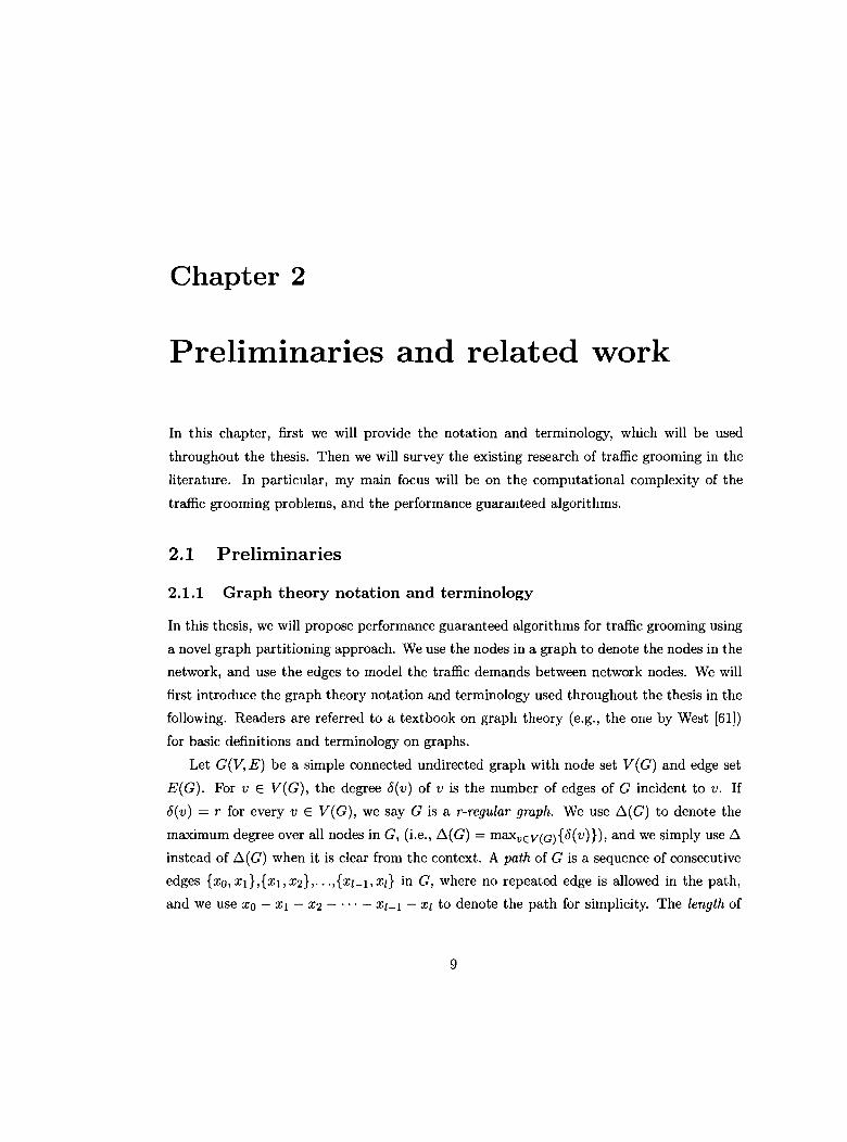
2 Preliminaries and related work
2.1.1 Graph theory notation and terminology
2.1.2 Approximation algorithm .
2.2 Related work .
2.2.1 Traffic grooming in UPSR networks
2.1 Preliminaries . . . . . . . . . .
9
9
9
11
12
12
vi
2.2.2 Traffic grooming in BLSR networks 18
3 Traffic Grooming in UPSR networks 21
3.1 Problem formulation 21
3.2 Algorithms ..... 23
3.2.1 Skeleton and skeleton cover 24
3.2.2 Algorithm kEP . . . . . 26
3.2.3 Algorithm SpanT-Euler 36
3.3 Empirical results 43
3.4 Summary · ... 44
4 Traffic grooming in UPSR with regular traffic 49
4.1 Problem formulation . . . . 49
4.2 Computational complexity. 50
4.2.1 NP-hardness · ... 51
4.2.2 The non-existence of FPTAS 53
4.2.3 NP-hardness for restricted k . 54
4.3 An approximation algorithm 56
4.4 Empirical results 60
4.5 Summary · ... 64
5 Min-Max and Max Throughput traffic grooming 68
5.1 Problem formulation . . . . . . . . . . . 69
5.2 Min-Max k-Edge-Partitioning Problem. 70
5.2.1 NP-hardness · .......... 71
5.2.2 A linear time (kt1+ 2)-approximation algorithm 73
5.2.3 Special case: all-to-all traffic pattern . . . . . . 77
5.3 Maximum Connectivity k-Edge-Partitioning Problem. 79
5.3.1 NP-hardness · ............ 80
5.3.2 A (k + 1)-approximation algorithm . 80
5.3.3 Special case: all-to-all traffic pattern 83
5.4 Empirical results 85
5.5 Summary · ... 86
vii
6 Traffic grooming in BLSR networks 90
6.1 Definitions and problem formulations. 90
6.2 Algorithms ............... 92
6.2.1 Algorithms for the MMkEPH problem 92
6.2.2 Algorithms for the MaxCkEPH problem. 95
6.3 Empirical results 96
6.4 Summary .... 97
7 Discussion for future work 99
7.1 Traffic grooming in mesh networks 99
7.1.1 Related work .. 99
7.1.2 Future research. .105
7.2 Traffic grooming in other topologies .106
7.2.1 Related work .. .106
7.2.2 Future research. .108
8 Concluding remarks 109
Bibliography 111
viii
List of Figures
1.1
1.2
1.3
2.1
2.2
2.3
3.1
3.2
3.3
3.4
3.5
3.6
3.7
3.8
3.9
3.10
3.11
3.12
4.1
4.2
4.3
4.4
4.5
Node architecture without/with WADM..
A traffic grooming example.
Optical ring topologies.
A graph partitioning example.. . . . . . . . . .
Examples of graphes with at most three edges.
Illustration of constructing the open tree of a traffic graph.
Pseudo code of Algorithm kEP. . . . . . .
Illustration of constructing skeleton cover.
Marking nodes of Ttl and white edge types.
Updating Ttl. . .
Extracting skeletons from Ttl.
Subroutine for finding a skeleton cover S of G.
A tree with height two.
Skeleton extraction.
Pseudo code of Algorithm SpanT-Euler.
Empirical results on graphs with n = 36 nodes.
Empirical results on graphs with n = 48 nodes.
Empirical results on graphs with n = 60 nodes.
An example: graph G with ~ = 4 and the corresponding 4-regular graph G*.
Pseudo code of Algorithm Regular-Euler. . .
Algorithm Regular-Euler: empirical results on graphs with n = 36 nodes.
Algorithm Regular-Euler: empirical results on graphs with n = 24 nodes.
Algorithm Regular_Euler: empirical results on graphs with n = 48 nodes.
ix
3
4
7
14
15
17
27
28
29
31
32
33
35
40
42
45
46
47
53
59
61
62
63
4.6 Average performance vs. worst case upper bound of Regular-Euler on graphs
with n = 36 nodes. . . . . . . . . . . . . . . . . . . . . . . . . . . . . . . . . . 65
4.7 Average performance vs. worst case upper bound of Regular_Euler on graphs
with n = 24 nodes. . . . . . . . . . . . . . . . . . . . . . . . . . . . . . . .. 66
4.8 Average performance vs. worst case upper bound of Regular_Euler on graphs
with n = 48 nodes. . . . . . . . . . . . . . . . . . . . . . . . . . . . . . . . . . 67
5.1 An example: graph G and the corresponding bipartite graph Gb' 74
5.2 An example: Marking edges of Gb • . . . • • • . 75
5.3 Pseudo code for Algorithm MinMax_Grooming. 76
5.4 Pseudo code for Algorithm MaxConnectivity_Grooming. 82
5.5 Performance of Algorithm MinMax_Grooming for n = 36 and d = 0.6 . 86
5.6 Performance of Algorithm MinMax_Grooming for n = 48 and d = 0.5 . 87
5.7 Performance of Algorithm MinMax_Grooming for n = 60 and d = 0.5 . 87
5.8 Performance of Algorithm MaxConnectivity_Grooming for n = 36, k = 4,
and d = 0.6. . . . . . . . . . . . . . . . . . . . . . . . . . . . . . . . . . . .. 88
5.9 Performance of Algorithm MaxConnectivity_Grooming for n = 48, k = 4,
and d = 0.5 " 88
5.10 Performance of Algorithm MaxConnectivity_Grooming for n = 60, k = 4,
and d = 0.5. . . . . . . . . . . . . . . . . . . . . . . . . . . . . . . . . . . .. 89
6.1 Pseudo code for Algorithm MinMaxJIyper .
6.2 Performance of Algorithm MinMaxJIyper for n = 36 and t = 0.6 .
6.3 Performance of Algorithm MinMax_Hyper for n = 48 and t = 0.6 .
6.4 Performance of Algorithm MinMax_Hyper for n = 60 and t = 0.6 .
x
93
96
97
98
Chapter 1
Overview
1.1 Background
1.1.1 WDM technology
With the explosive growth of the Internet traffic, and the increasing demand for delay
sensitive multimedia network applications, it has been a challenging issue for the telecom
munication infrastructure to provide sufficient bandwidth capacity for numerous Internet
users. The introduction of fiber optics brings a bandwidth revolution to solve this problem.
Optical fibers provide huge bandwidth capacity, which can be up to 50 terabits per second.
However, the electronic network end devices usually operate on a speed of a few gigabits per
second [45]. To eliminate the huge opto-electronic bandwidth mismatch, the bandwidth of
an optical fiber is split into a number of non-overlapping wavelength channels, each of which
operates at an electronic data rate. This multiplexing is known as the Wavelength Division
Multiplexing (WDM) technology, which is widely used in optical networks to exploit the
tremendous bandwidth capacity inherent in optical fibers.
1.1.2 Traffic grooming
In a WDM optical network, every optical fiber supports multiple wavelength channels,
each of which has a bandwidth up to a few gigabit per second. However, the bandwidth
requirement of an individual network traffic demand is normally much lower than the ca
pacity provided by a wavelength channel. Therefore multiple low-rate traffic demands are
1
CHAPTER 1. OVERVIEW 2
usually multiplexed together to share a high-speed wavelength channel during the trans
mission, and demultiplexed when arriving at corresponding destinations. The multiplex
ing/demultiplexing is known as tmffic grooming, and the maximum number of traffic de
mands that can be multiplexed into a wavelength channel is called grooming factor. For
example, four OC-3 (155.52 Mbps) traffic demands can be multiplexed into a wavelength
channel operated at OC-12 (622.08 Mbps), giving a grooming factor of 4.
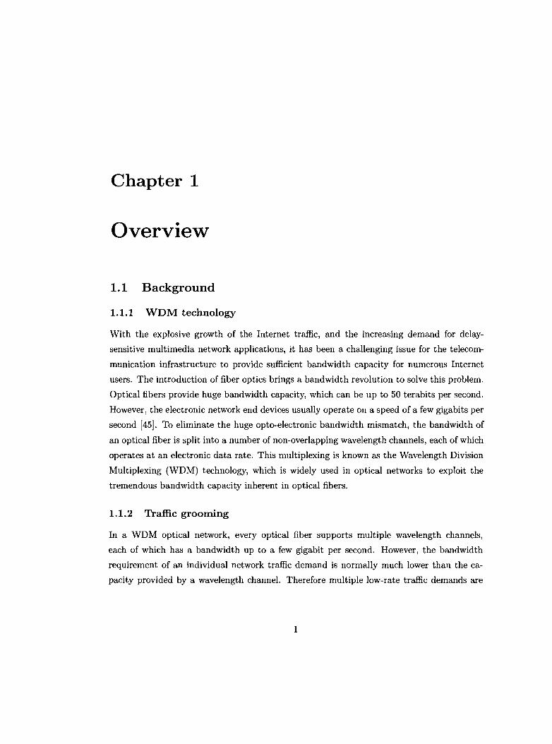
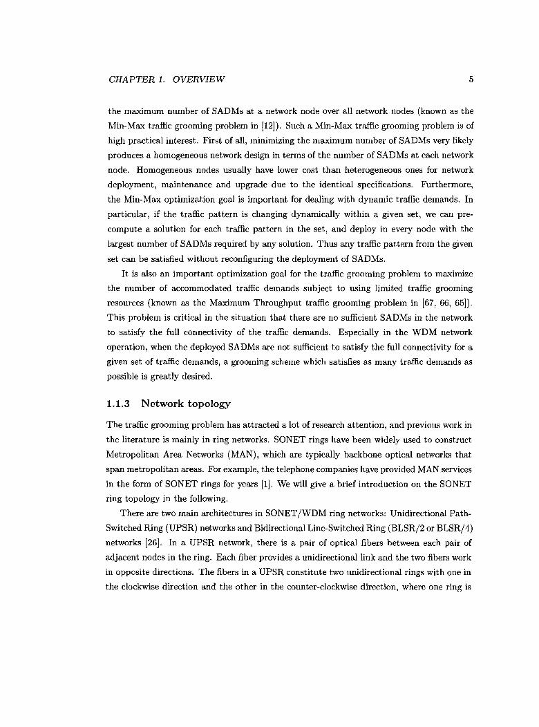
In SONET/WDM networks, traffic grooming is carried out by SONET Add-Drop Mul
tiplexers (SADM), where one SADM is used to multiplex/demultiplex the traffic demands
into/from a specific wavelength channel at each network node. With the emerging optical
devices such as Wavelength Add-Drop Multiplexers (WADM), it is possible for a network
node to optically bypass a wavelength channel if the wavelength does not carry any traffic
ending at the node. Therefore, at each network node SADMs are needed only for the wave
lengths which carry traffic from/to the node. Figure 1.1 shows the difference between an
optical network node architecture without WADM (Figure 1.1(a)) and a node architecture
with WADM (Figure 1.1(b)), where it is assumed that only wavelength A2 carries low-rate
traffic demands from/to the network node shown in the Figure. It is clear that the number
of SADMs can be decreased by deploying one WADM at each network node, and arrang
ing the multiplexing/demultiplexing carefully. SADMs are expensive network devices and
dominate the cost of SONET/WDM networks, so it is critical to minimize the number of
SADMs in the SONET/WDM network design by utilizing the optical bypass capability of
WADMs. Generally speaking, to reduce the number of SADMs, low-rate traffic demands
should be groomed in a way to yield as many optical bypasses as possible.
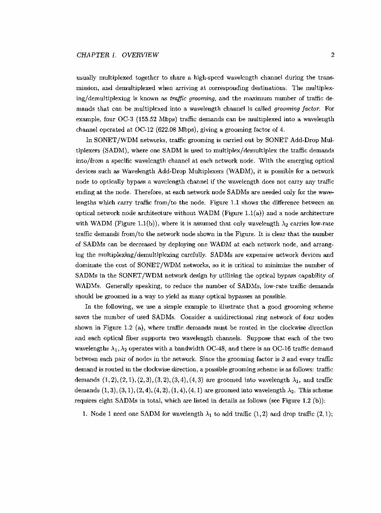
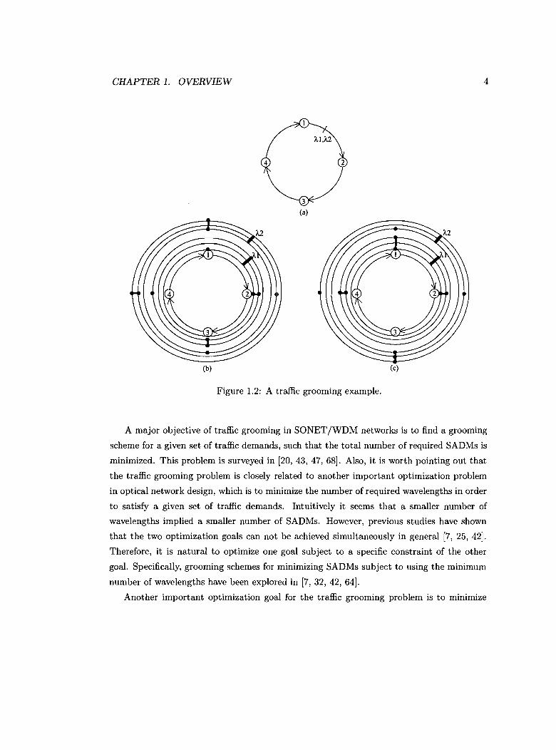
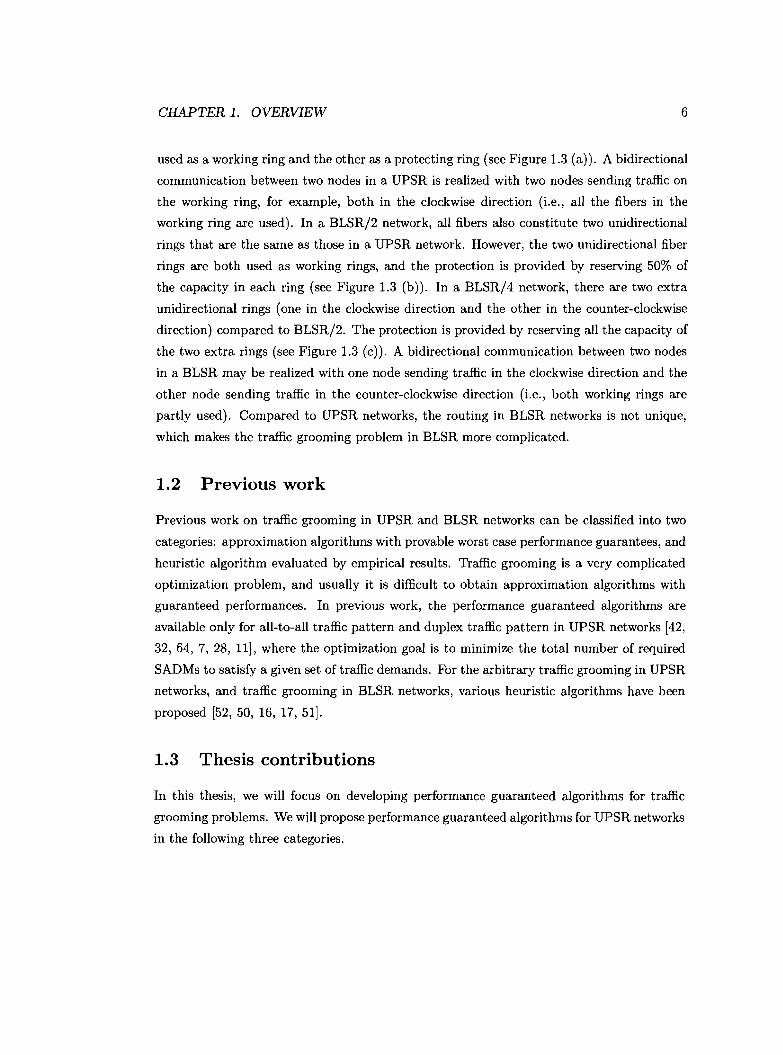
In the following, we use a simple example to illustrate that a good grooming scheme
saves the number of used SADMs. Consider a unidirectional ring network of four nodes
shown in Figure 1.2 (a), where traffic demands must be routed in the clockwise direction
and each optical fiber supports two wavelength channels. Suppose that each of the two
wavelengths AI, A2 operates with a bandwidth OC-48, and there is an OC-16 traffic demand
between each pair of nodes in the network. Since the grooming factor is 3 and every traffic
demand is routed in the clockwise direction, a possible grooming scheme is as follows: traffic
demands (1,2), (2, 1), (2,3), (3, 2), (3,4), (4,3) are groomed into wavelength AI, and traffic
demands (1,3), (3, 1), (2,4), (4, 2), (1,4), (4,1) are groomed into wavelength A2. This scheme
requires eight SADMs in total, which are listed in details as follows (see Figure 1.2 (b)):
1. Node 1 need one SADM for wavelength Al to add traffic (1,2) and drop traffic (2,1);
CHAPTER 1. OVERVIEW
,----------- A,I
1--------- ~
i -----~:~~----------------------------~
a network node
(a)
-----F==f------ A,I-~---A,2
A3------------
I r-'-----'--,IIIIIIII
-----------------------------~
a network node(b)
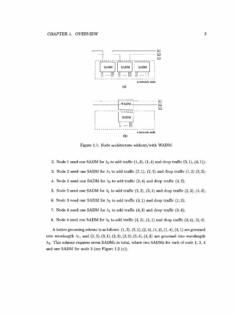
Figure 1.1: Node architecture without/with WADM.
3
2. Node 1 need one SADM for A2 to add traffic (1,3), (1,4) and drop traffic (3,1), (4,1));
3. Node 2 need one SADM for Al to add traffic (2,1), (2,3) and drop traffic (1,2) (3,2);
4. Node 2 need one SADM for A2 to add traffic (2,4) and drop traffic (4,2);
5. Node 3 need one SADM for Al to add traffic (3,2), (3,4) and drop traffic (2,3), (4,3);
6. Node 3 need one SADM for A2 to add traffic (3,1) and drop traffic (1,3);
7. Node 4 need one SADM for Al to add traffic (4,3) and drop traffic (3,4);
8. Node 4 need one SADM for A2 to add traffic (4,2), (4,1) and drop traffic (2,4), (1,4).
A better grooming scheme is as follows: (1,2), (2, 1), (2,4), (4,2), (1,4), (4, 1) are groomed
into wavelength AI, and (1,3), (3, 1), (2,3), (3,2), (3,4), (4,3) are groomed into wavelength
A2. This scheme requires seven SADMs in total, where two SADMs for each of node 1, 2, 4
and one SADM for node 3 (see Figure 1.2 (c)).
CHAPTER 1. OVERVIEW 4
(b)
Figure 1.2: A traffic grooming example.
(c)
A major objective of traffic grooming in SONET/WDM networks is to find a grooming
scheme for a given set of traffic demands, such that the total number of required SADMs is
minimized. This problem is surveyed in [20, 43, 47, 68]. Also, it is worth pointing out that
the traffic grooming problem is closely related to another important optimization problem
in optical network design, which is to minimize the number of required wavelengths in order
to satisfy a given set of traffic demands. Intuitively it seems that a smaller number of
wavelengths implied a smaller number of SADMs. However, previous studies have shown
that the two optimization goals can not be achieved simultaneously in general [7, 25, 42].
Therefore, it is natural to optimize one goal subject to a specific constraint of the other
goal. Specifically, grooming schemes for minimizing SADMs subject to using the minimum
number of wavelengths have been explored in [7, 32, 42, 64].
Another important optimization goal for the traffic grooming problem is to minimize
CHAPTER 1. OVERVIEW 5
the maximum number of SADMs at a network node over all network nodes (known as the
Min-Max traffic grooming problem in [12]). Such a Min-Max traffic grooming problem is of
high practical interest. First of all, minimizing the maximum number of SADMs very likely
produces a homogeneous network design in terms of the number of SADMs at each network
node. Homogeneous nodes usually have lower cost than heterogeneous ones for network
deployment, maintenance and upgrade due to the identical specifications. Furthermore,
the Min-Max optimization goal is important for dealing with dynamic traffic demands. In
particular, if the traffic pattern is changing dynamically within a given set, we can pre
compute a solution for each traffic pattern in the set, and deploy in every node with the
largest number of SADMs required by any solution. Thus any traffic pattern from the given
set can be satisfied without reconfiguring the deployment of SADMs.
It is also an important optimization goal for the traffic grooming problem to maximize
the number of accommodated traffic demands subject to using limited traffic grooming
resources (known as the Maximum Throughput traffic grooming problem in [67, 66, 65]).
This problem is critical in the situation that there are no sufficient SADMs in the network
to satisfy the full connectivity of the traffic demands. Especially in the WDM network
operation, when the deployed SADMs are not sufficient to satisfy the full connectivity for a
given set of traffic demands, a grooming scheme which satisfies as many traffic demands as
possible is greatly desired.
1.1.3 Network topology
The traffic grooming problem has attracted a lot of research attention, and previous work in
the literature is mainly in ring networks. SONET rings have been widely used to construct
Metropolitan Area Networks (MAN), which are typically backbone optical networks that
span metropolitan areas. For example, the telephone companies have provided MAN services
in the form of SONET rings for years [IJ. We will give a brief introduction on the SONET
ring topology in the following.
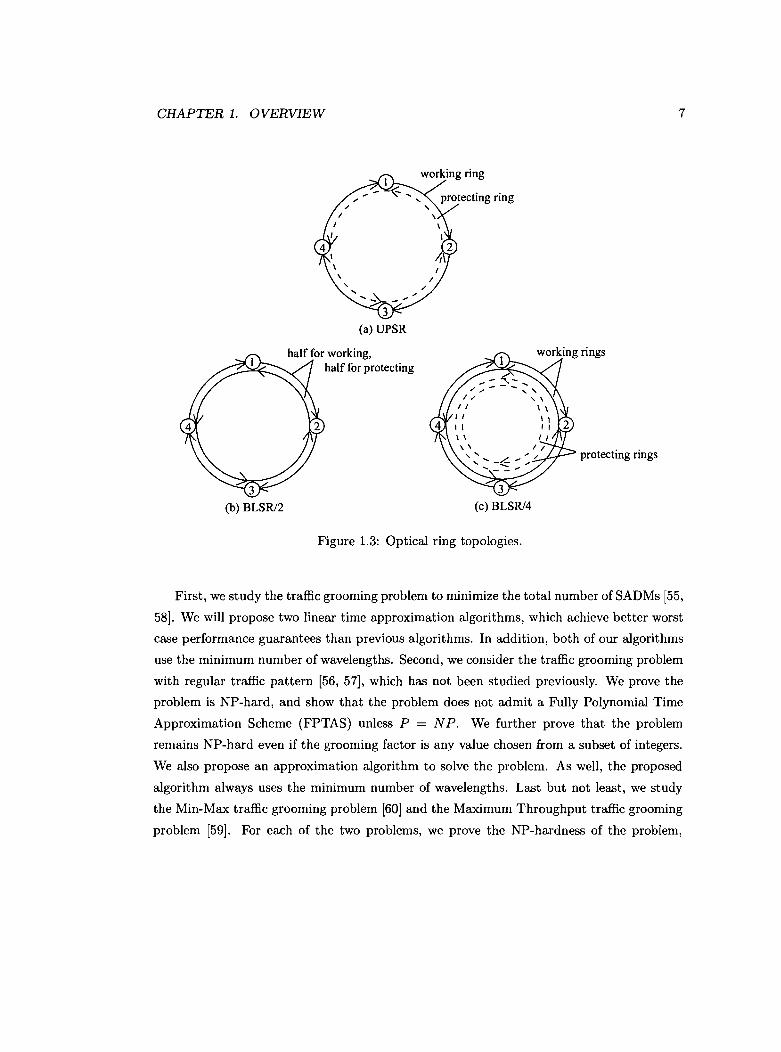
There are two main architectures in SONET/WDM ring networks: Unidirectional Path
Switched Ring (UPSR) networks and Bidirectional Line-Switched Ring (BLSR/2 or BLSR/4)
networks [26J. In a UPSR network, there is a pair of optical fibers between each pair of
adjacent nodes in the ring. Each fiber provides a unidirectional link and the two fibers work
in opposite directions. The fibers in a UPSR constitute two unidirectional rings with one in
the clockwise direction and the other in the counter-clockwise direction, where one ring is
CHAPTER 1. OVERVIEW 6
used as a working ring and the other as a protecting ring (see Figure 1.3 (a)). A bidirectional
communication between two nodes in a UPSR is realized with two nodes sending traffic on
the working ring, for example, both in the clockwise direction (i.e., all the fibers in the
working ring are used). In a BLSR/2 network, all fibers also constitute two unidirectional
rings that are the same as those in a UPSR network. However, the two unidirectional fiber
rings are both used as working rings, and the protection is provided by reserving 50% of
the capacity in each ring (see Figure 1.3 (b)). In a BLSR/4 network, there are two extra
unidirectional rings (one in the clockwise direction and the other in the counter-clockwise
direction) compared to BLSR/2. The protection is provided by reserving all the capacity of
the two extra rings (see Figure 1.3 (c)). A bidirectional communication between two nodes
in a BLSR may be realized with one node sending traffic in the clockwise direction and the
other node sending traffic in the counter-clockwise direction (Le., both working rings are
partly used). Compared to UPSR networks, the routing in BLSR networks is not unique,
which makes the traffic grooming problem in BLSR more complicated.
1.2 Previous work
Previous work on traffic grooming in UPSR and BLSR networks can be classified into two
categories: approximation algorithms with provable worst case performance guarantees, and
heuristic algorithm evaluated by empirical results. Traffic grooming is a very complicated
optimization problem, and usually it is difficult to obtain approximation algorithms with
guaranteed performances. In previous work, the performance guaranteed algorithms are
available only for all-to-all traffic pattern and duplex traffic pattern in UPSR networks [42,
32, 64, 7, 28, 11]' where the optimization goal is to minimize the total number of required
SADMs to satisfy a given set of traffic demands. For the arbitrary traffic grooming in UPSR
networks, and traffic grooming in BLSR networks, various heuristic algorithms have been
proposed [52, 50,16,17,51].
1.3 Thesis contributions
In this thesis, we will focus on developing performance guaranteed algorithms for traffic
grooming problems. We will propose performance guaranteed algorithms for UPSR networks
in the following three categories.
CHAPTER 1. OVERVIEW
3
(a) UPSR
7
3
(b) BLSR/2
3
(c) BLSR/4
Figure 1.3: Optical ring topologies.
protecting rings
First, we study the traffic grooming problem to minimize the total number of SADMs [55,
58]. We will propose two linear time approximation algorithms, which achieve better worst
case performance guarantees than previous algorithms. In addition, both of our algorithms
use the minimum number of wavelengths. Second, we consider the traffic grooming problem
with regular traffic pattern [56, 57], which has not been studied previously. We prove the
problem is NP-hard, and show that the problem does not admit a Fully Polynomial Time
Approximation Scheme (FPTAS) unless P = N P. We further prove that the problem
remains NP-hard even if the grooming factor is any value chosen from a subset of integers.
We also propose an approximation algorithm to solve the problem. As well, the proposed
algorithm always uses the minimum number of wavelengths. Last but not least, we study
the Min-Max: traffic grooming problem [60] and the Maximum Throughput traffic grooming
problem [59]. For each of the two problems, we prove the NP-hardness of the problem,
CHAPTER 1. OVERVIEW 8
and propose an approximation algorithm. We also study the all-to-all traffic pattern, and
present algorithms achieving solutions only constant factors away from the optimal ones.
In addition, we will study the traffic grooming problem in BLSR networks. As the
topology changes from UPSR to BLSR, the complexity of the traffic grooming problem
increases. There is no performance guaranteed algorithm available so far. We will extend
our algorithms proposed for UPSR networks to design efficient heuristic algorithms for traffic
grooming in BLSR networks.
1.4 Thesis organization
This thesis is organized as follows: In Chapter 2, we first present preliminaries, and then
summarize the previous work that is closely related to our research. In Chapter 3, we pro
pose algorithms for the traffic grooming problem to minimize the total number of required
SADMs in UPSR networks, and obtain improved guaranteed performance than previous
algorithms. In Chapter 4 we study traffic grooming in UPSR networks with regular traffic
pattern, which has not be considered before. In Chapter 5 we consider the Min-Max traf
fic grooming problem and the Maximum Throughput traffic grooming problem in UPSR
networks. We analyze the computational complexity for both problems, and propose per
formance guaranteed algorithms for them. In Chapter 6, we study traffic grooming in BLSR
networks. Future extensions to traffic grooming in other network topologies are discussed
in Chapter 7. The final chapter concludes the thesis.
Chapter 2
Preliminaries and related work
In this chapter, first we will provide the notation and terminology, which will be used
throughout the thesis. Then we will survey the existing research of traffic grooming in the
literature. In particular, my main focus will be on the computational complexity of the
traffic grooming problems, and the performance guaranteed algorithms.
2.1 Preliminaries
2.1.1 Graph theory notation and terminology
In this thesis, we will propose performance guaranteed algorithms for traffic grooming using
a novel graph partitioning approach. We use the nodes in a graph to denote the nodes in the
network, and use the edges to model the traffic demands between network nodes. We will
first introduce the graph theory notation and terminology used throughout the thesis in the
following. Readers are referred to a textbook on graph theory (e.g., the one by West [61])
for basic definitions and terminology on graphs.
Let G(V, E) be a simple connected undirected graph with node set V(G) and edge set
E(G). For v E V(G), the degree 8(v) of v is the number of edges of G incident to v. If
8(v) = r for every v E V(G), we say G is a r-regular gmph. We use 6(G) to denote the
maximum degree over all nodes in G, (i.e., 6(G) = maxvEV(G) {8(v)}), and we simply use 6
instead of 6(G) when it is clear from the context. A path of G is a sequence of consecutive
edges {xo, Xd,{XI, X2}," .,{Xl-I, Xl} in G, where no repeated edge is allowed in the path,
and we use Xo - Xl - X2 - ... - Xl-I - Xl to denote the path for simplicity. The length of
9
CHAPTER 2. PRELIMINARIES AND RELATED WORK 10
a path is the number of edges in the path, and we use l-path to denote a path of length l.
The two nodes at which a path starts and terminates are called end-nodes of the path, and
all other nodes on the path are called mid-nodes. A simple path is a path with no repeated
node. An Euler path of graph G is a path which uses each edge of G exactly once, and
a connected graph has an Euler path if and only if it has at most two odd-degree nodes.
A component of G is a maximal connected sub-graph of G. The edge connectivity of G is
defined to be the minimum number of edges whose deletion from G partitions G into at
least two components.
A tree T is a connected graph with IV(T) I - 1 edges, and a spanning tree of G is a tree
that contains all nodes of G. A rooted spanning tree of G is a spanning tree of G where a
node r is specified as the root. For any node u other than root r in a rooted spanning tree
T, the parent of u, denoted as up, is the node adjacent to u on the path from u to r in T.
For any node u in T, a descendant of u is a node x such that u is on the unique path from
x to r, and the length of the unique path from x to u in tree T is denoted by dT (x, u).
For any node u in T, the depth of u is defined as dT (u, r). For a node u in T, the subtree
induced by node u and all its descendants is denoted by Tu , and node u is the root of Tu .
The depth of Tu is defined as dT(u, r) (Le., the depth of node u). The height of Tu , denoted
as h(Tu ), is defined as max{dT(x, u)jx E V(Tu )}. A tree is called trivial if the tree contains
only one node.
For a simple undirected graph G(V, E), a matching M of G is a set of edges of G such
that no two edges of M share a node in common. We say a node is saturated by matching
M if the node is an end-node of some edge in M. If a matching saturates every node of G,
then it is a perfect matching. For graph G and a function b : V (G) --> Z+, a b-matching M
is a set of edges in G such that each node v of G appears in at most b(v) edges of M. A
maximum b-matching is a b-matching with the maximum cardinality, and can be computed
in polynomial time for a simple graph G [23]. An edge coloring of G is a coloring of the
edges of G such that adjacent edges receive different colors. For graph G and a function
f : V (G) --> Z+, an f -coloring is to assign a color for each edge in E(G), such that at most
f(v) edges incident to a node v receive the same color. It is proved that an f-coloring with
at most !:i.f + 1 colors can be computed in polynomial time for a simple graph G, where
!:i.f = maxvEv(G)f8(v)/f(v)1 [30]. The edge coloring is a special case of the f-coloring,
where f(v) = 1 for each v E V(G).
A clique of graph G is a complete sub-graph of G, and the size of the clique is the number
CHAPTER 2. PRELIMINARIES AND RELATED WORK 11
of nodes in the clique. A star, denoted as S, is a tree with one node having degree IV(S) [-I
and the others having degree 1. The node of degree IV(S) 1-1 is called the center of star S.
A bipartite graph G(U, V, E) is a graph whose node set can be divided into two non-empty
sets U (G) and V (G) such that for every edge {u, v} E E (G), one of nodes u, v is in U (G)
and the other is in V (G).
2.1.2 Approximation algorithm
For any NP-hard optimization problem, there is no polynomial time algorithm to compute
an optimal solution unless P = N P. So much effort has been put into developing polyno
mial time algorithms to find near-optimal solutions whose values are close to the value of
an optimal solution. We call such a near-optimal solution an approximate solution, and an
algorithm that produces approximate solutions an approximation algorithm. The following
formal definitions of the approximate solution, approximation algorithm, and approxima
tion ratio are from the book by Cormen et al. [18].
Approximate Solution: for an optimization problem fl, a feasible solution with the value
close to the value of an optimal solution is an approximate solution of fl.
Approximation Algorithm: for an optimization problem fl, a polynomial time algorithm
that generates approximate solutions is an approximation algorithm of fl.
Any algorithm that produces approximate solutions for problem fl can be called an
approximation algorithm. How to evaluate approximation algorithms is important. Gen
erally speaking, good approximation algorithms should be efficient (polynomial time) and
produce solutions with values as close to the optimum as possible. Concept approximation
ratio is widely used to evaluate approximation algorithms. In the following, we assume that
a solution always has a positive value.
Approximation Ratio: an approximation algorithm A for an optimization problem flhas an approximation ratio of p(n) if for any instance of fl with size n, the value C of any
approximate solution produced by the approximation algorithm satisfies
C C*max{ C*' C} ~ p(n),
CHAPTER 2. PRELIMINARIES AND RELATED WORK
where C· is the value of an optimal solution.
12
This definition applies to both maximization and minimization problems. For a maxi
mization problem, 0 < C :::; C·, and C· /C gives the approximation ratio. For a minimization
problem, 0 < C· :::; C, and C/C· gives the approximation ratio. Therefore, the approxi
mation ratio of an approximation algorithm is at least 1, and the approximation ratio of
an optimal algorithm is exactly 1. An approximation algorithm with a large approximation
ratio may return a solution that is much worse than an optimal solution. Reducing the
approximation ratio as close to 1 as possible is a major goal of developing approximation
algorithms.
For a minimization problem Il, an algorithm A is called a Polynomial Time Approxi
mation Scheme (PTAS) if its running time, for any instance of Il and a parameter of fixed
E > 0, is bounded by a polynomial in the size of the instance, and the value C of any solution
produced by A satisfies .g. :::; 1 + E, where C· is the value of an optimal solution. A Fully
Polynomial Time Approximation Scheme (FPTAS) is a PTAS for which the running time
is bounded polynomially in both the size of the problem instance and ~.
2.2 Related work
2.2.1 Traffic grooming in UPSR networks
Traffic grooming is a complicated optimization problem, and usually it is difficult to obtain
polynomial time optimal algorithms or even approximation algorithms with guaranteed
performances. So far, the performance guaranteed algorithms are available only for all-to
all traffic pattern and duplex traffic pattern.
All-to-all traffic pattern
For the all-to-all traffic pattern, there is a traffic demand (x, y) from node x to node y for
every pair of nodes x and y in the UPSR network. A traffic demand is unitary if it requires
one unit of bandwidth. Without loss of generality, we assume that every traffic demand
is unitary, since otherwise we can split a traffic into multiple unitary sub-traffic. We call
(x, y) and (y, x) a duplex traffic pair, and use {x, y} to denote the unitary duplex traffic pair
(x,y) and (y,x). In the UPSR network, every duplex pair of unitary traffic occupies a full
CHAPTER 2. PRELIMINARIES AND RELATED WORK 13
cycle with one unit of bandwidth. Such a full cycle is called a primitive cycle, and up to k
primitive cycles can be groomed into one wavelength for a grooming factor of k.
For the all-to-all traffic grooming with grooming factor k = 4 and k = 16, Chiu and
Modiano [42] derived lower bounds on the number of SADMs, and Hu [32J provided the
optimal solutions. For an arbitrary grooming factor k, lower bounds and heuristics were
proposed by Chiu and Modiano [42J, and Zhang and Qiao [64], where the heuristics are
evaluated by computer simulations, yet their approximation ratios are not given.
By formulating the traffic grooming problem as a graph partitioning problem, Bermond
and Coudert [7J optimally solved the all-to-all traffic grooming problem in UPSR networks
if the grooming factor k is a practical value or in the infinite congruence classes of values.
The graph partitioning formulation is based on the following fact which has been assumed
implicitly in [7J: for any grooming scheme (}, a grooming scheme (}' can be constructed such
that (}' always puts each unitary duplex pair into one primitive cycle and (}' uses no more
SADMs than (} (we will give the explicit proof for this claim in the next chapter). Therefore
for the all-to-all traffic pattern, we can always put each duplex pair into a primitive cycle,
and concentrate on grooming primitive cycles into wavelengths so that the number of used
SADMs is minimized. In the graph partitioning approach proposed by [7], the all-to-all
traffic pattern is represented by an undirected complete graph G(V, E) called traffic graph,
where V (G) represents the set of nodes in the UPSR network and each edge in E(G) between
node x and y represents the duplex traffic pair {x,y}. Then the all-to-all traffic grooming
problem is formulated as the following k-Edge-Partitioning problem of the traffic graph:
For a positive integer k ::; IE(G) I, partition the edge set E(G) into a collection of sub
sets E = {E1 , E 2 , ... ,Ew} (where U~lEi = E(G) and Ep n Eq = 0 for p -:j:. q), such that
IEil ::; k for each E i E E and L:EiEt:IVi I is minimized, where Vi is the set of nodes in the
sub-graph induced by edge set Ei.
It is observed that integer k corresponds to the grooming factor, W corresponds to
the number of used wavelengths, each induced sub-graph corresponds to a wavelength, and
L:EiEt:IViI corresponds to the total number of used SADMs. We will take the example given
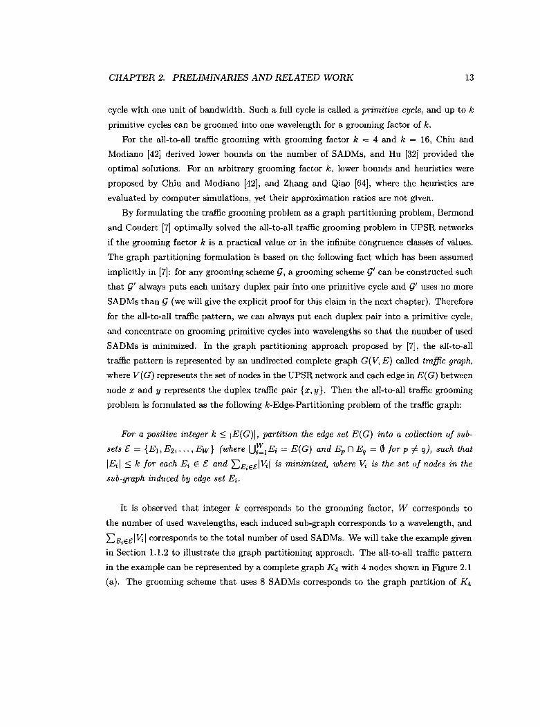
in Section 1.1.2 to illustrate the graph partitioning approach. The all-to-all traffic pattern
in the example can be represented by a complete graph K4 with 4 nodes shown in Figure 2.1
(a). The grooming scheme that uses 8 SADMs corresponds to the graph partition of K4
CHAPTER 2. PRELIMINARIES AND RELATED WORK 14
shown in Figure 2.1 (b), and the grooming scheme that uses 7 SADMs corresponds to the
graph partition shown in Figure 2.1 (c) .
.....-----------:l.2
4 3
(a)
I:=)' IX'4 3 4 3
sub-graph I sub-graph 2(b)
]~7~' 1~'443
sub-graph I sub-graph 2(c)
Figure 2.1: A graph partitioning example.
Bermond and Coudert [7J tackled the graph partitioning problem using the techniques
of design theory [15J. Their results improve and unify all the previous results on the all-to
all traffic grooming in UPSR networks. In particular, they completely or partially solved
the cases that k = 3,4,5,6,8,9,10,16 and various congruence classes for other values of
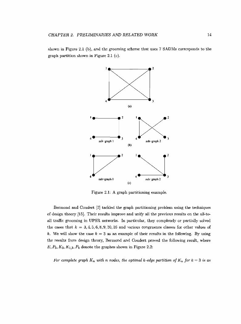
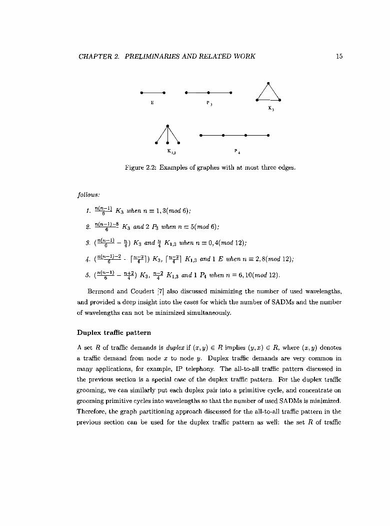
k. We will show the case k = 3 as an example of their results in the following. By using
the results from design theory, Bermond and Coudert proved the following result, where
E, P3, K3, Kl,3, P4 denote the graphes shown in Figure 2.2:
For complete graph K n with n nodes, the optimal k-edge partition of K n for k = 3 is as
CHAPTER 2. PRELIMINARIES AND RELATED WORK
• • • • • LE P3
K 3
11\ • • • •
K i ,3 P 4
Figure 2.2: Examples of graphes with at most three edges.
follows:
1. n(n6-1) K3 whenn:=l,3(mod6);
2. n(n~1)-8 K3 and 2 P3 when n:= 5(mod 6);
3. (n(n6-1) - ~) K3 and ~ K 1,3 when n:= O,4(mod 12);
4. (n(n~1)-2 - rn 42 1) K3, rn 421Kl,3 and 1 E when n:= 2,8(mod 12);
5. (n(n6-1) - n!2) K3, n42 K1,3 and 1 P4 when n:= 6, 10(mod 12).
15
Bermond and Coudert [7] also discussed minimizing the number of used wavelengths,
and provided a deep insight into the cases for which the number of SADMs and the number
of wavelengths can not be minimized simultaneously.
Duplex traffic pattern
A set R of traffic demands is duplex if (x,y) E R implies (y,x) E R, where (x,y) denotes
a traffic demand from node x to node y. Duplex traffic demands are very common in
many applications, for example, IP telephony. The all-to-all traffic pattern discussed in
the previous section is a special case of the duplex traffic pattern. For the duplex traffic
grooming, we can similarly put each duplex pair into a primitive cycle, and concentrate on
grooming primitive cycles into wavelengths so that the number of used SADMs is minimized.
Therefore, the graph partitioning approach discussed for the all-to-all traffic pattern in the
previous section can be used for the duplex traffic pattern as well: the set R of traffic
CHAPTER 2. PRELIMINARIES AND RELATED WORK 16
demand pairs is represented by an undirected graph G(V, E), where V (G) represents the set
of nodes in the UPSR network, and there is an edge in E(G) between node x and y if and
only if {x, y} E R. The only difference from the all-to-all traffic grooming is that we now
consider the k-Edge-Partitioning problem on arbitrary traffic graphs rather than complete
traffic graphs.
For arbitrary traffic graphs, Goldschmidt et at. [28] proved that the k-Edge-Partitioning
problem is NP-hard. The NP-hardness proof is based on the reduction from the Edge
Partition into Triangles (EPT) problem, which is known to be NP-hard [31] and the decision
version of the EPT problem is stated as follows:
Edge-Partition into Triangles (EPT) Problem
Instance: An undirected graph G(V, E).
Question: Is there a partition of E(G) into pairwise disjoint subsets El, E2, ... ,EIE(Gll/3'
such that each E i induces a triangle?
For the NP-completeness proof, it is shown that any given instance of the EPT problem
can be transformed to an instance of the k-Edge-Partitioning problem on the same graph
with k = 3, such that the instance has a solution if and only if the original EPT instance
has a solution.
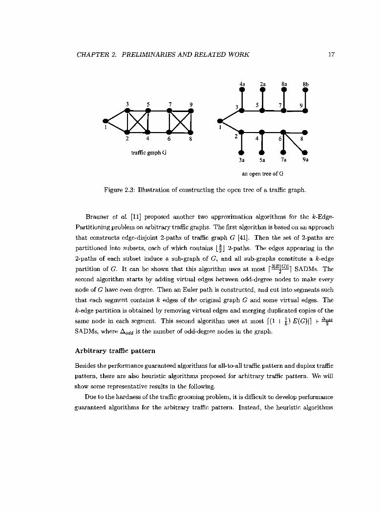
Goldschmidt et at. [28] also proposed an approximation algorithm for the k-Edge-Partitioning
problem on arbitrary traffic graphs. The algorithm first transforms a traffic graph G
into an open tree as follows: it computes a spanning tree T of G. Then for every edge
{u,v} E E(G)\E(T), it re-labels node vasa new node and attaches edge {u,v} to node
u in T. Figure 2.3 illustrates how to construct an open tree for a given graph G. It
is clear that an open tree of G has the same number of edges as G, and has duplicated
copies for some nodes of G. Then the open tree is partitioned into subtrees such that
r~l :::; IE(T')I :::; k for each subtree T'. For each subtree, a sub-graph G i of G can be
obtained by merging duplicated copies of the same node in the subtree. All such sub
graphs together constitute a k-edge partition of G. It is clear that the number of edges
IE(Gi)1 in each sub-graph Gi satisfies r~l :::; IE(Gi)1 :::; k. For each sub-graph Gi , the
number of nodes IV(Gi )1 :::; IE(Gi)1 + 1, where the equation holds if and only if Gi is a
tree. Since each sub-graph contains at least r~l edges, the total number of sub-graphs
is at most I~~~ll :::; 2lEfll. Therefore, the total number of nodes over all sub-graphs is
Ei IV(Gi) I :::; Ei(IE(Gi)1 + 1) :::; IE(G)I + 2IE~Gll = IE(G)I(l + ~), which means the algo
rithm uses at most rIE(G)I(l + ~)l SADMs.
CHAPTER 2. PRELIMINARIES AND RELATED WORK 17
3 5 7 9
~M9a7a
2a
5a
4
4a
3a
8a 8b
;,3.._ ....5__-~7.-l
864
traffic graph G
2
an open tree ofG
Figure 2.3: Illustration of constructing the open tree of a traffic graph.
Brauner et ai. [11] proposed another two approximation algorithms for the k-Edge
Partitioning problem on arbitrary traffic graphs. The first algorithm is based on an approach
that constructs edge-disjoint 2-paths of traffic graph G [41]. Then the set of 2-paths are
partitioned into subsets, each of which contains l~J 2-paths. The edges appearing in the
2-paths of each subset induce a sub-graph of G, and all sub-graphs constitute a k-edge
partition of G. It can be shown that this algorithm uses at most r3IEJG)ll SADMs. The
second algorithm starts by adding virtual edges between odd-degree nodes to make every
node of G have even degree. Then an Euler path is constructed, and cut into segments such
that each segment contains k edges of the original graph G and some virtual edges. The
k-edge partition is obtained by removing virtual edges and merging duplicated copies of the
same node in each segment. This second algorithm uses at most r(l + VIE(G)Il + ~~dd
SADMs, where tlodd is the number of odd-degree nodes in the graph.
Arbitrary traffic pattern
Besides the performance guaranteed algorithms for all-to-all traffic pattern and duplex traffic
pattern, there are also heuristic algorithms proposed for arbitrary traffic pattern. We will
show some representative results in the following.
Due to the hardness of the traffic grooming problem, it is difficult to develop performance
guaranteed algorithms for the arbitrary traffic pattern. Instead, the heuristic algorithms
CHAPTER 2. PRELIMINARIES AND RELATED WORK 18
evaluated by simulations have been proposed by a lot of research papers, among which the
work by Wan et ai. [52] can be considered as a representative one.
For an arbitrary traffic pattern, the algorithm in [52] uses a two-step approach to solve
the traffic grooming problem: generation of primitive cycles and grooming of primitive
cycles. In the first step to generate primitive cycles, the set of traffic demands are partitioned
into groups such that the routing paths for the traffic demands within any group do not
overlap. Therefore, the traffic demands in each group can be put into one primitive cycle.
The cost of each group (or primitive cycle) is defined as the number of different nodes
appearing as the endpoints of the routing paths contained in the primitive cycle, and the
cost of a partition is defined as the sum of the costs of the primitive cycles within this
partition. The objective of the first step is then to find a valid partition of the arbitrary
traffic set into groups such that the partition has the minimum cost.
In the second step to groom primitive cycles, primitive cycles are groomed into high
speed wavelength channels such that the number of primitive cycles in each wavelength
channel is no more than the grooming factor k. The cost of each wavelength channel is
defined as the number of different nodes appearing as the endpoints of the routing paths
in the primitive cycles groomed in the wavelength channel, that is, the number of SADMs
required for the wavelength. Therefore, the objective of the second step is to groom a set
of primitive cycles such that the number of required SADMs is minimized. Wan et ai. [52]
give a performance guaranteed sub-algorithm for each of the two steps. However, there is
no proof (and it is difficult to prove) on a set of solutions of the first step, based on which
optimal solutions for the whole problem can be derived in the second step. Therefore, the
worst case performance of the two-step approach in [52] is not guaranteed.
2.2.2 Traffic grooming in BLSR networks
For BLSR networks, usually a similar two-step approach as the one in [52] is used to solve
the traffic grooming problem, where the first step is to generate primitive cycles and the
second step is to groom primitive cycles into wavelength channels. Traffic grooming in
BLSR networks is more complicated than traffic grooming in UPSR networks, and there
is no performance guaranteed algorithms so far even for all-to-all traffic pattern. However,
there has been research work which proposes performance guaranteed sub-algorithms for
each of the two steps. We will briefly review such algorithms for both all-to-all traffic
pattern and arbitrary traffic pattern in this section.
CHAPTER 2. PRELIMINARIES AND RELATED WORK
All-to-all traffic pattern
19
Wan [50] studied the all-to-all traffic grooming on BLSR networks for grooming factor
k = 1,2, and 4. Colbourn and Wan [17], and Colbourn and Ling [16] solved the case k = 8
using the techniques of design theory [15]. All of these works use the same two-step approach
to tackle the traffic grooming problem: the first step is to generate primitive cycles and the
second step is to groom primitive cycles, where the goal for the first step is to minimize the
number of primitive cycles, and the goal of the second step is to minimize the number of
SADMs.
For the first step, Wan [50] proposed the an approach to achieve the minimum number
of primitive cycles: when the number n of nodes in the BLSR network is even, ~2 primitive
cycles are constructed, where r~21 primitive cycles are in the clockwise direction and the
other l ~2 J ones are in the counterclockwise direction; when n is odd, n2
4-1 primitive cycles
are constructed, where rn2
811 primitive cycles are in each of the clockwise and counter
clockwise directions. For the second step, they model the primitive cycles constructed in
the first step as a complete graph with a loop on each node, and then formulate the primi
tive cycle grooming into a graph partitioning problem: partition the edges of the graph into
sub-graphs, each of which contains at most k edges (where loops are counted as edges when
n is odd, and counted as half-edges when n is even), such that the total SADM cost of all
sub-graphs is minimized. Based on this graph partitioning approach, the cases k = 1,2,4,8
are studied in [16, 17, 50] to achieve the minimum number of SADMs given the primitive
cycles obtained in the first step.
It is worth pointing out that the two-step approach does not guarantee that the number of
used SADMs is optimum even the optimal solution can be achieved for each step individually.
This is because that the two steps are not completely independent, and the solution to the
first step might affect how the second step can be solved optimally.
Arbitrary traffic pattern
The two-step approach is used for arbitrary traffic grooming in BLSR networks as well [51].
The first step is to generate primitive cycles and the second step is to groom primitive
cycles obtained from the first step. Two versions of the problem are considered in [51],
where the first version is that each traffic stream has a predetermined routing, and the
second version is that the routing of each traffic stream is not given in advance. It is proved
CHAPTER 2. PRELIMINARiES AND RELATED WORK 20
that both versions are NP-hard for any fixed grooming factor k. For both versions, various
performance guaranteed algorithms are developed to solve primitive cycle generation sub
problem or the primitive cycle grooming sub-problem individually. However, it is difficult
to derive performance guaranteed results for the whole traffic grooming algorithm as well.
Chapter 3
Traffic Grooming in UPSR
networks
Minimizing the total number of required SADMs, as a major optimization goal of the traffic
grooming problem, has been shown very challenging. It is NP-hard even for Unidirectional
Path-Switched Ring (UPSR) networks with unitary duplex traffic pattern. In this chapter,
we propose two linear time approximation algorithms for this NP-hard problem based on a
novel graph partitioning approach. Both algorithms achieve better worst case performances
than previous algorithms. We show that the upper bounds obtained by our algorithms
are very close to the lower bounds for some instances. In addition, both of our algorithms
use the minimum number of wavelengths, which are precious resources as well in optical
networks. We also conduct extensive simulations to evaluate the average performances of
our algorithms.
3.1 Problem formulation
Recall that in UPSR networks, a pair of unitary duplex traffic occupies a full cycle with one
unit of bandwidth. Such a full cycle is called a primitive cycle, and up to k primitive cycles
can be groomed into one wavelength for a grooming factor of k. To illustrate the graph
partition formulation more clearly, we prove the following theorem first.
Theorem 1 For any grooming scheme (}, there exists a grooming scheme (}' such that (}'
always puts every unitary duplex pair into a primitive cycle and (}' uses no more SADMs
21
CHAPTER 3. TRAFFIC GROOMING IN UPSR NETWORKS
than g.
22
Proof: Recall that a primitive cycle denotes a full cycle with unitary bandwidth capacity
in the SONET/WDM ring network, that is, a wavelength channel along the ring network
consists of k primitive cycles for a grooming factor of k. In the UPSR network, a primitive
cycle can carry exactly one unitary duplex traffic pair. We consider any grooming scheme
9 as the following two-step procedure: the first step is a packing scheme P that puts traffic
into primitive cycles, and the second step is a clustering scheme C that puts primitive cycles
into wavelengths. We use pi to denote the special packing scheme that puts each duplex
traffic pair into a primitive cycle. For any grooming scheme 9 consisting of a packing scheme
p and a clustering scheme C, if P = pi, g' can be constructed such that g'=g. Otherwise,
it is observed that pi uses no more primitive cycles than P. We call traffic demand (i,j) a
long demand if its routing path in the UPSR has length at least ~ (where n is the number of
nodes in the UPSR), and a short demand otherwise. It is noticed that a duplex pair contains
at least one long demand. Now we define the following function f to map primitives cycles
used in pi to those used in P:
1. For each primitive cycle x used in pi that carries a long demand (i, j) and a short
demand (j, i), and suppose y is the primitive cycle used in P that carries (i, j), we
define f(x) = y.
2. For each primitive cycle x used in pi that carries two long demands (i,j) and (j, i) (in
this case, n is even, and the length of the routing paths for both (i,j) and (j, i) is ~),
and suppose Yl is the primitive cycle used in P carrying (i, j) and yz is the primitive
cycle used in P carrying (j, i), we define either f(x) = Yl or f(x) = yz.
The above function f is an injective function, since no primitive cycle can carry more than
one long demand from different duplex traffic pairs. Now we construct grooming scheme g'with packing scheme pi, and clustering scheme C' as follows: two primitive cycles Xl and Xz
used in pi are put into the same wavelength if and only if f(Xl) and f(xz) are put into the
same wavelength in C. Since f is an injective function, it is clear g' uses no more SADMs
than g. 0
According to Theorem 1, for a set R of unitary duplex traffic demand pairs in UPSR
networks, we can always put each pair into a primitive cycle, and concentrate on grooming
primitive cycles into wavelengths so that the number of required SADMs is minimized. That
CHAPTER 3. TRAFFIC GROOMING IN UPSR NETWORKS 23
is, the traffic grooming problem can be solved by partitioning R into subsets, each of which
contains at most k duplex pairs, and use one wavelength to carry each subset. For each
node involved in at least one duplex pair of a subset carried by a wavelength A, we need one
SADM for wavelength A at the node, and minimizing the total number of required SADMs
is equivalent to minimizing the sum of the number of distinct nodes involved in each subset.
As we mentioned in Chapter 2, the traffic grooming problem in UPSR networks with
unitary duplex traffic pattern has been formulated as the following k-Edge-Partitioning
problem to develop approximation algorithms [11, 28]:
k-Edge-Partitioning Problem
Instance: A traffic graph G(V,E) and integer k::; IE(G)I.
Objective: Partition the edge set E(G) into a collection of subsets £ = {E l , E2 , ••. , Ew}
(where U~lEi = E(G) and Ep n Eq = 0 for p =f q), such that IEil ::; k for each Ei E £ and
LEiE£IViI is minimized, where Vi is the set of nodes in the sub-graph induced by edge set
Ei·
In this formulation, a simple undirected graph G(V, E), called traffic graph, is con
structed to represent the set R of unitary duplex traffic demand pairs, where node set V(G)
denotes the set of network nodes in the UPSR and there is an edge {x, y} E E(G) between
node x and y if and only if there exists a unitary duplex pair {x, y} E R (when it is clear
in the context, we use {x,y} to denote either an edge in the graph or a unitary duplex pair
in R). It is observed that integer k corresponds to the grooming factor, W corresponds
to the number of required wavelengths, and LEiE£IViI corresponds to the total number of
required SADMs. We also notice that f/E1G) I1is a lower bound on the number of required
wavelengths (Le., f'E1G)[1 ::; W).
3.2 Algorithms
For arbitrary traffic graphs, the k-Edge-Partitioning problem has been proved NP-hard [28]
and two approximation algorithms have been proposed in [11, 28J. Intuitively, to achieve
good solutions for the k-Edge-Partitioning problem, we need to partition traffic graph G into
sub-graphs of at most k edges such that each sub-graph contains as few nodes as possible.
One key observation is that given a fixed number of edges of G, a sub-graph induced by
the edges more likely contains fewer nodes if there are fewer components in the sub-graph.
This is the basic idea behind the algorithms in [11, 28]. The algorithm in [28] guarantees
CHAPTER 3. TRAFFIC GROOMING IN UPSR NETWORKS 24
that each sub-graph is connected, while every sub-graph might contain only rk/2l edges in
the worst case. The algorithm in [11] does not guarantee that each sub-graph is connected,
instead it guarantees that the total number of components over all sub-graphs is bounded
above and each sub-graph contains exactly kedges.
In this section, we propose two linear time approximation algorithms for the k-Edge
Partitioning problem based on a novel graph partitioning approach. Both algorithms utilize
the similar idea as that of the algorithm in [11], and they guarantee the total number
of components over all sub-graphs is bounded above. Our algorithms use at most r(l +i) jE(G) Il + llV~G)1J SADMs and achieve a better upper bound than previous algorithms
of [11] and [28J as long as t:!J.odd > IV~G)I (i.e., the traffic graph has a small number of even
degree nodes) andl~fg~f > ~ (i.e., the traffic graph is relatively dense), respectively. It can
be shown that our upper bounds are very close to the lower bounds for some instances. In
addition, it is worth pointing out that both of our algorithms use the minimum number
r'EtG)'l of wavelengths. We also conduct simulations to evaluate the performances of our
algorithms, and the results show that our algorithms outperform the previous algorithms.
3.2.1 Skeleton and skeleton cover
To solve the k-Edge-Partitioning problem, our algorithms use a novel approach of partition
ing traffic graph G into special sub-graphs called skeletons. A skeleton 5 of G is a connected
sub-graph of G that consists of a backbone and a set of branches, where the backbone is a
path of G, and each branch is an edge of G such that at least one end-node of the edge is
in the backbone. We say a branch {u, v} is attached to node u in the backbone if u is a
node in the backbone (notice that a branch may be attached to two nodes in the backbone).
The length of a skeleton 5, denoted as l(5), is the length of its backbone. A skeleton cover
S of graph G is a set of skeletons {51, 52 ... , 5 j } which form an edge partition of G (i.e.,
U{=d E(5i ) = E(G) and E(5p ) n E(5q) = 0 for p =F q), where j is the size of the skeleton
cover (i.e., j = lSI). We call f : V(G) -t S a characteristic function of skeleton cover S if
f maps each node u E V(G) to a unique skeleton 5 j E S for some 5 j with u E V(5 j ). For
each node u E V(G) and f(u) = 5 j , u is called a characteristic node of 5 j • The following
properties on skeletons and skeleton covers play key roles in our algorithms.
Proposition 2 For any skeleton 5 and integer t with 0 < t < IE(5)1, 5 can be partitioned
into two skeletons 51 and 52, such that IE(51)1 = t and IE(52)1 = IE(5)1- t.
CHAPTER 3. TRAFFIC GROOMING IN UPSR NETWORKS 25
Proof: We prove. this proposition by constructing Sl and S2 from S. Assume that the
backbone of S is U1 - U2 - ... - UI(Sl+1, where U1 and UI(Sl+1 are the two end-nodes of the
backbone. Initially Sl is empty (i.e., IE(Sl)1 = 0). We start from i = 1 to check whether
the number of branches attached to Ui is less than t - IE(Sl)l. If so, we remove all such
branches and edge {ui,ui+d from S, add them into Sl, and repeat the same process for
next node Ui+1 in the backbone. Otherwise we remove t - IE(Sl)1 such branches from S,
add them into Sl, and terminate with S2 = S\Sl. It is easy to see that eventually both Sl
and S2 are skeletons with IE(Sl)1 = t and IE(S2)1 = IE(S)I - t. 0
By Proposition 2, it is easy to transform a skeleton cover to a k-edge partition of G with
exactly k edges in each sub-graph except the last one (note that some sub-graphs might be
disconnected). Especially we have the following proposition for any skeleton cover.
Proposition 3 Any skeleton coverS = {Sl, S2,"" Sj} of graph G can be transformed into
a k-edge partition £ = {E1, ... , Ew} of G with W = rlE1GliliEil = k for 1 ~ i < W, and
2:EiEf IViI ~ f(l + t)IE(G)1l + (j - 1).
Proof: Let Si and ti be the end-nodes of the backbone of each skeleton Si E S. We
can connect Sl, ... , Sj into one skeleton S* by adding (j - 1) virtual edges {ti, si+d for
1 ~ i ~ j - 1. According to Proposition 2, S* can be cut into W skeletons {Si, S2, ... , Sty},
where W = f'E1Gl' l, each skeleton S1 (1 ~ i ~ W -1) contains exactly k edges of G and
ji virtual edges, and Sty contains at most k edges of G and jw virtual edges. We have
2:~1 ji = j - 1 since the total number of added virtual edges is j - 1. For a skeleton of
k +ji edges, the maximum number of nodes in the skeleton is k +ji +1. Therefore the set of
skeletons {Si, S2' ... , Sty} becomes a k-edge-partition £ = {E1 , ••• , Ew} of G after deleting
virtual edges, and
w 1L IViI ~ IE(G)I + Lji + W = f(l + k)IE(G)ll + (j - 1).EiEf i=l
o
Proposition 4 For any skeleton cover S = {Sl, S2, ...} of graph G and integer t, if there
exists a characteristic function f of S such that at most one skeleton in S contains less than
t characteristic nodes, then lSI ~ flV\Gl'l·Proof: Assume that at most one skeleton contains x (where x < t) characteristic nodes.
By the definition of the characteristic function, each node U E V( G) is a characteristic
CHAPTER 3. TRAFFIC GROOMING IN UPSR NETWORKS 26
node for exactly one skeleton in S. Since IV(G)I is the total number of nodes, we have
x + (ISI- l)t ~ IV(G)I, which implies that lSI ~ l(IV~Gll + ttl)J ~ rlV(tGlll 0
By Proposition 4, if we can construct a skeleton cover S of G such that the number of
characteristic nodes in each skeleton is bounded below, then the size of S is bounded above.
After S is transformed to a k-edge partition of G, the total number of components over all
sub-graphs in the k-edge partition will be bounded above.
In the following we propose two linear time approximation algorithms for the k-Edge
Partitioning problem based on constructing skeleton covers of the traffic graph. The first
algorithm kEP constructs a skeleton cover with size at most rlV~Gl'l for traffic graph G.
The second algorithm SpanT..Euler constructs a skeleton cover with the help of Euler path
construction, and achieves an upper bound that is at least as good as the one obtained
by Algorithm kEP. In addition, both Algorithm kEP and Algorithm SpanT_Euler use the
minimum number r,E1Gl'l of wavelengths.
3.2.2 Algorithm kEP
The algorithm
We first give a brief review on the previous algorithms [11, 28] for the k-Edge-Partitioning
problem, since our algorithm is designed in order to overcome the deficiencies of these
algorithms. The algorithm in [11] first adds virtual edges between odd-degree nodes to
make every node of G have even degree. Then an Euler path is constructed, and cut into
segments such that each segment contains k edges of the original graph G and some virtual
edges. A k-edge partition is obtained by removing virtual edges and merging duplicated
copies of the same node in each segment. The algorithm in [28] transforms traffic graph G
into an open tree as follows: it first computes a spanning tree T of G. Then for every edge
{u, v} E E(G)\E(T), renames node v as U v and attaches edge {u, uv } to node u in T. It is
clear that an open tree of G has the same edge set as G, and has duplicated copies for some
nodes of G. Then the open tree is partitioned into subtrees such that r~l ~ IE(T')I ~ k
for each subtree T', and a k-edge partition can be obtained by merging duplicated copies of
the same node in each subtree.
As we mentioned previously, in order to achieve good solutions for the k-Edge-Partitioning
problem, the obtained k-edge partition should contain as few components as possible over
all sub-graphs. For the algorithm in [11], the number of components depends on the number
CHAPTER 3. TRAFFIC GROOMING IN UPSR NETWORKS 27
of odd-degree nodes that can be as large as IV(G)I in the worst case. In addition, the adja
cent edges in G might be separated far away in the constructed Euler path, therefore each
sub-graph G* in the obtained k-edge partition could be sparse in term of the ratio j~tg:H.
Similar problem might occur for the algorithm in [28], since the adjacent edges in G might
be separated far away in the constructed open tree.
We propose Algorithm kEP for the k-Edge-Partitioning problem. Our algorithm first
constructs a skeleton cover S of traffic graph G. Then all the constructed skeletons are
connected together by adding virtual edges to form a virtual skeleton, which covers all the
edges of G exactly once. Then the virtual skeleton can be partitioned into segments, each
of which contains exactly k edges of G and some virtual edges according to Proposition 2.
We notice that duplicated copies of a node of G might exist in a segment. In order to get a
k-edge partition of G, we need to merge duplicated copies of the same node as follows: for
any two edges {v,w} and {x,y} in a segment, assume v and x are two duplicated copies of
the same node in G (i.e., {v,w} and {x,y} are adjacent edges in G), we delete edge {x,y}
from the segment and add a new edge {v, y} into the segment. Therefore, a k-edge partition
can be obtained by removing virtual edges and merging duplicated copies of the same node
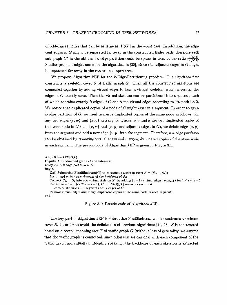
in each segment. The pseudo code of Algorithm kEP is given in Figure 3.1.
Algorithm kEP(G,k)Input: An undirected graph G and integer k.Output: A k-edge partition of G.begin
Call Subroutine FindSkeleton(G) to construct a skeleton cover S = {Sl, ... , S.};Let Ui and Vi be the end-nodes of the backbone of Si;Connect SI, ... , S. into one virtual skeleton S· by adding (8 - 1) virtual edges {Vi, Ui+l} for 1 ~ i ~ s - 1;Cut S· into l = i(IE(S·)I- s + 1)/k1 = iIE(G)I/k1 segments such that
each of the first l - 1 segments has k edges of G;Remove virtual edges and merge duplicated copies of the same node in each segment;
end.
Figure 3.1: Pseudo code of Algorithm kEP.
The key part of Algorithm kEP is Subroutine FindSkeleton, which constructs a skeleton
cover S. In order to avoid the deficiencies of previous algorithms [11, 28], S is constructed
based on a rooted spanning tree T of traffic graph G (without loss of generality, we assume
that the traffic graph is connected, since otherwise we can deal with each component of the
traffic graph individually). Roughly speaking, the backbone of each skeleton is extracted
CHAPTER 3. TRAFFIC GROOMING IN UPSR NETWORKS 28
from E(T), and edges of E(G)\E(T) are attached as branches (a few edges from E(T)
might also be attached as branches). Thus each skeleton is very likely to be a relatively
dense sub-graph of G. In addition, we construct S in a way that each skeleton in S has at
least four characteristic nodes (it can be easily show that there exist instances where four
characteristic nodes is the maximum worst case guarantee we can obtain), which guarantees
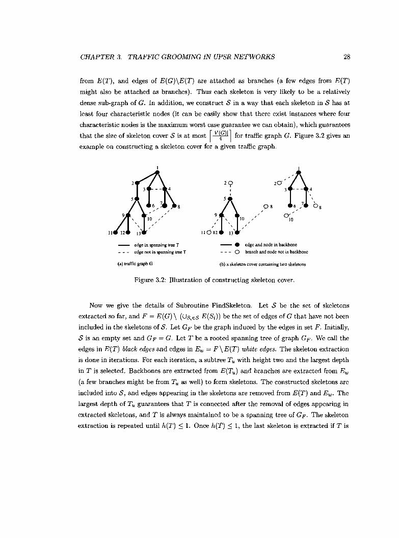
that the size of skeleton cover S is at most rlV~G)'l for traffic graph G. Figure 3.2 gives an
example on constructing a skeleton cover for a given traffic graph.
II
CY10
edge in spanning tree T
edge not in spanning tree T
(a) traffic graph G
-. edge and node in backbone
- - - 0 branch and node not in backbone
(b) a skeleton cover containing two skeletons
Figure 3.2: Illustration of constructing skeleton cover.
Now we give the details of Subroutine FindSkeleton. Let S be the set of skeletons
extracted so far, and F = E(G) \ (USiES E(Si)) be the set of edges of G that have not been
included in the skeletons of S. Let GF be the graph induced by the edges in set F. Initially,
S is an empty set and GF = G. Let T be a rooted spanning tree of graph GF. We call the
edges in E(T) black edges and edges in Ew = F \ E(T) white edges. The skeleton extraction
is done in iterations. For each iteration, a subtree Tu with height two and the largest depth
in T is selected. Backbones are extracted from E(Tu ) and branches are extracted from Ew
(a few branches might be from Tu as well) to form skeletons. The constructed skeletons are
included into S, and edges appearing in the skeletons are removed from E(T) and Ew . The
largest depth of Tu guarantees that T is connected after the removal of edges appearing in
extracted skeletons, and T is always maintained to be a spanning tree of GF. The skeleton
extraction is repeated until h(T) ::; 1. Once h(T) ::; 1, the last skeleton is extracted if T is
CHAPTER 3. TRAFFIC GROOMING IN UPSR NETWORKS 29
........ white edge
(a) marking nodes in T.white edge {x, y} with xmarked
o unmarked node
(b) white edge {x, y} withx in T. and y not in T.
• marked node
(c) white edge {x, y} with x and y in To
-- black edge
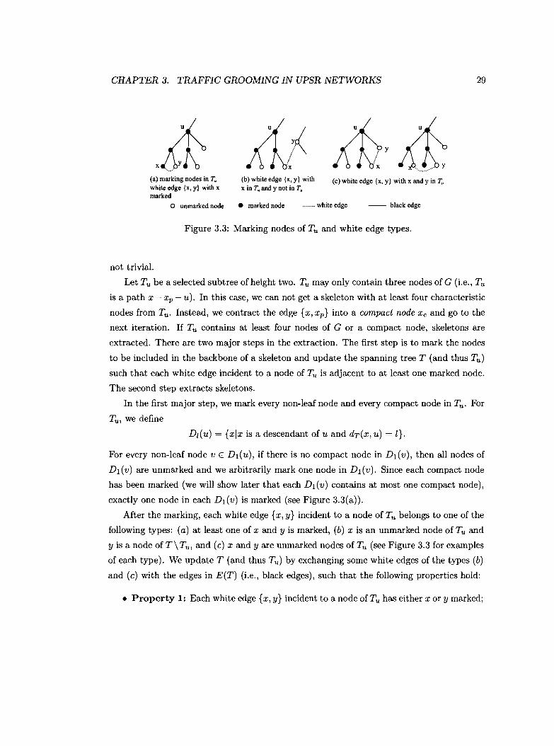
Figure 3.3: Marking nodes of Tu and white edge types.
not trivial.
Let Tu be a selected subtree of height two. Tu may only contain three nodes of G (Le., Tu
is a path x - xp - u). In this case, we can not get a skeleton with at least four characteristic
nodes from Tu . Instead, we contract the edge {x,xp } into a compact node Xc and go to the
next iteration. If Tu contains at least four nodes of G or a compact node, skeletons are
extracted. There are two major steps in the extraction. The first step is to mark the nodes
to be included in the backbone of a skeleton and update the spanning tree T (and thus Tu )
such that each white edge incident to a node of Tu is adjacent to at least one marked node.
The second step extracts skeletons.
In the first major step, we mark every non-leaf node and every compact node in Tu . For
Tu , we define
D l (u) = {xix is a descendant of u and dT(x, u) = l}.
For every non-leaf node v E Dl (u), if there is no compact node in Dl (v), then all nodes of
D1(v) are unmarked and we arbitrarily mark one node in D1(v). Since each compact node
has been marked (we will show later that each D1(v) contains at most one compact node),
exactly one node in each D1(v) is marked (see Figure 3.3(a)).
After the marking, each white edge {x, y} incident to a node of Tu belongs to one of the
following types: (a) at least one of x and y is marked, (b) x is an unmarked node of Tu and
y is a node of T\Tu , and (c) x and y are unmarked nodes of Tu (see Figure 3.3 for examples
of each type). We update T (and thus Tu ) by exchanging some white edges of the types (b)
and (c) with the edges in E(T) (i.e., black edges), such that the following properties hold:
• Property 1: Each white edge {x,y} incident to a node ofTu has either x or y marked;
CHAPTER 3. TRAFFIC GROOMING IN UPSR NETWORKS
• Property 2: T is always maintained as a spanning tree of GF;
• Property 3: The height of Tu is not increased after the updating.
30
Property 1 guarantees that each white edge incident to a node of T can be included in a
skeleton as a branch. Property 2 guarantees that no edge will be missed when extracting
skeletons, since every edge of GF is either in the spanning tree T (i.e., a black edge) or
incident to a node in T (i.e., a white edge). Property 3 is used to make the second major
step (i.e., the skeleton extraction step) less complicated, as we only need to consider a
subtree of height two. Based on the three properties above, the key in extracting a skeleton
is to find the backbone of the skeleton. From now on, when we say a skeleton S with a
backbone Xl - X2 - ... - X s is extracted, we mean that S is extracted with Xl - X2 - ... - X s
as the backbone, and all white edges incident to the nodes of the backbone as branches.
Then S is included into S and the edges of E(S) are deleted from GF.
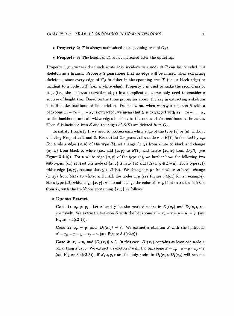
To satisfy Property 1, we need to process each white edge of the type (b) or (c), without
violating Properties 2 and 3. Recall that the parent of a node X E V (T) is denoted by xp '
For a white edge {x,y} of the type (b), we change {x,y} from white to black and change
{xp,x} from black to white (i.e., add {x,y} to E(T) and delete {xp,x} from E(T)) (see
Figure 3.4(b)). For a white edge {x,y} of the type (c), we further have the following two
sub-types: (c1) at least one node of {x, y} is in DI(u) and (c2) x, y E D2(U). For a type (c1)
white edge {x,y}, assume that y E DI(u). We change {x,y} from white to black, change
{x,xp } from black to white, and mark the nodes x,y (see Figure 3.4(c1) for an example).
For a type (c2) white edge {x, y}, we do not change the color of {x, y} but extract a skeleton
from Tu with the backbone containing {x, y} as follows.
• Update-Extract
Case 1: xp =I- yp' Let x' and y' be the marked nodes in DI(xp) and DI(yp), re
spectively. We extract a skeleton S with the backbone x' - x p - x - y - yp - y' (see
Figure 3.4(c2-1)).
Case 2: x p = YP and IDI(xp)1 = 3. We extract a skeleton S with the backbone
x' - x p - x - y - xp - u (see Figure 3.4(c2-2)).
Case 3: xp = YP and IDI(xp)1 > 3. In this case, DI(xp) contains at least one node z
other than x', x, y. We extract a skeleton S with the backbone x' - xp - x - y - xp - z
(see Figure 3.4(c2-3)). If x',x,y,z are the only nodes in DI(xp), DI(xp) will become
CHAPTER 3. TRAFFIC GROOMING IN UPSR NETWORKS 31
(b) change {x, y} from white to black andchange {x, Xp} from black to white.
(c I) change {x, y} from white to black, change{x, xp} from black to white. and mark x, y.
~~. ~ '.~. ~x;:Xyh'0 x~1\
....... x .......~. y:x' y'
••.•..••••... Y
(c2-1) extract backbonex· -xpx-y-yP-y'
(c2-2) extract backbonex· -xpx-y-xp-u
(c2-3) extract backbonex I -xp.x-y-xp-z
• marked node
........ white edge
-- black edge
Figure 3.4: Updating Ttl.
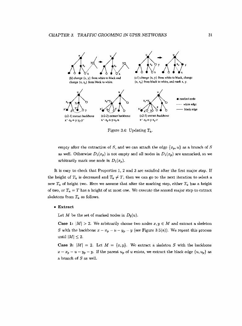
empty after the extraction of S, and we can attach the edge {xp , u} as a branch of S
as well. Otherwise D 1(xp ) is not empty and all nodes in D 1(xp ) are unmarked, so we
arbitrarily mark one node in D1(xp ).
It is easy to check that Properties 1, 2 and 3 are satisfied after the first major step. If
the height of Ttl is decreased and Ttl f= T, then we can go to the next iteration to select a
new Ttl of height two. Here we assume that after the marking step, either Ttl has a height
of two, or Ttl = T has a height of at most one. We execute the second major step to extract
skeletons from Ttl as follows.
• Extract
Let M be the set of marked nodes in D2 (u).
Case 1: IMI > 2. We arbitrarily choose two nodes X, y E M and extract a skeleton
S with the backbone X - x p - u - yp - y (see Figure 3.5(a)). We repeat this process
until IMI :::; 2.
Case 2: IMI = 2. Let M = {x,y}. We extract a skeleton S with the backbone
x - xp - u - yp - y. If the parent up of u exists, we extract the black edge {u,up} as
a branch of S as well.
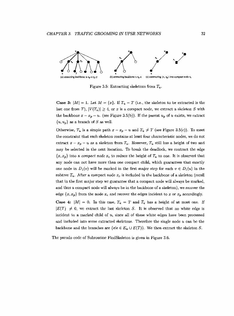
CHAPTER 3. TRAFFIC GROOMING IN UPSR NETWORKS 32
u
x Y(a) extracting backbone x-x,.-u-yp-y
x(b) extracting backbone x-x,.-u
x(c) contracting {x. x,.} into compact node ""
Figure 3.5: Extracting skeletons from Tu .
Case 3: IMI = 1. Let M = {x}. If Tu = T (i.e., the skeleton to be extracted is the
last one from T), JV(Tu ) I ~ 4, or x is a compact node, we extract a skeleton S with
the backbone x - xp - u. (see Figure 3.5(b)). If the parent up of u exists, we extract
{u, up} as a branch of S as well.
Otherwise, Tu is a simple path x - xp - u and Tu =I- T (see Figure 3.5(c)). To meet
the constraint that each skeleton contains at least four characteristic nodes, we do not
extract x - xp - u as a skeleton from Tu . However, Tu still has a height of two and
may be selected in the next iteration. To break the deadlock, we contract the edge
{x,xp } into a compact node Xc to reduce the height of Tu to one. It is observed that
any node can not have more than one compact child, which guarantees that exactly
one node in D 1(v) will be marked in the first major step for each v E Dl (u) in the
subtree Tu . After a compact node Xc is included in the backbone of a skeleton (recall
that in the first major step we guarantee that a compact node will always be marked,
and thus a compact node will always be in the backbone of a skeleton), we recover the
edge {x,xp } from the node Xc and recover the edges incident to x or xp accordingly.
Case 4: IMI = O. In this case, Tu = T and Tu has a height of at most one. If
IE(T)I =I- 0, we extract the last skeleton S. It is observed that no white edge is
incident to a marked child of u, since all of these white edges have been processed
and included into some extracted skeletons. Therefore the single node u can be the
backbone and the branches are {ele E Ew U E(T)}. We then extract the skeleton S.
The pseudo code of Subroutine FindSkeleton is given in Figure 3.6.
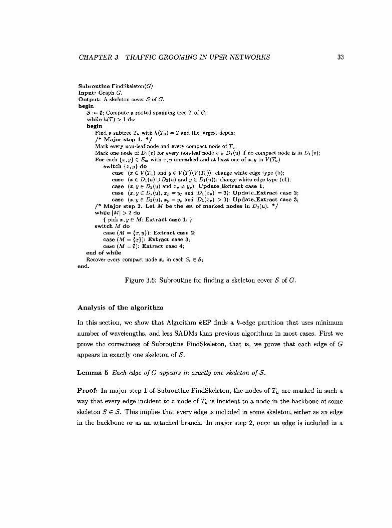
CHAPTER 3. TRAFFIC GROOMING IN UPSR NETWORKS
Subroutine FindSkeleton(G)Input: Graph G.Output: A skeleton cover S of G.begin
S := 0; Compute a rooted spanning tree T of G;while h(T) > 1 dobegin
Find a subtree T" with h(T,,) = 2 and the largest depth;/* Major step 1. */Mark every non-leaf node and every compact node of T,,;Mark one node of D 1(v) for every non-leaf node v E D 1 (u) if no compact node is in D 1 (v);For each {x, y} E Ew with x, y unmarked and at least one of x, yin V(T,,)
switch {x, y} docase (x E V(T,,) and y E V(T)\V(T,,)): change white edge type (b);case (x E D1(u) U D2 (u) and y E D1(u)): change white edge type (c1);case (x,y E D 2 (u) and X p cI yp): Update_Extract case 1;case (x,y E D 2 (u), x p = YP and ID1(xp)1 = 3): Update_Extract case 2;case (x,y E D 2 (u), X p = YP and ID1(xp)1 > 3): Update..Extract case 3;
/* Major step 2. Let M be the set of marked nodes in D2 (u). */while IMI > 2 do
{ pick x, y E M; Extract case 1; };switch M do
case (M = {x,y}): Extract case 2;case (M = {x}): Extract case 3;case (M = 0): Extract case 4;
end of whileRecover every compact node Xc in each S; E S;
end.
Figure 3.6: Subroutine for finding a skeleton cover S of G.
Analysis of the algorithm
33
In this section, we show that Algorithm kEP finds a k-edge partition that uses minimum
number of wavelengths, and less SADMs than previous algorithms in most cases. First we
prove the correctness of Subroutine FindSkeleton, that is, we prove that each edge of G
appears in exactly one skeleton of S.
Lemma 5 Each edge of G appears in exactly one skeleton of S.
Proof: In major step 1 of Subroutine FindSkeleton, the nodes of Ttl are marked in such a
way that every edge incident to a node of Ttl is incident to a node in the backbone of some
skeleton S E S. This implies that every edge is included in some skeleton, either as an edge
in the backbone or as an attached branch. In major step 2, once an edge is included in a
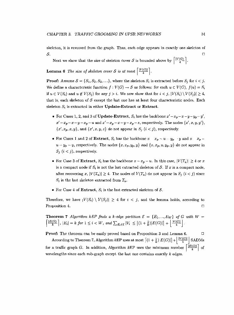
CHAPTER 3. TRAFFIC GROOMING IN UPSR NETWORKS 34
skeleton, it is removed from the graph. Thus, each edge appears in exactly one skeleton of
s. D
Next we show that the size of skeleton cover S is bounded above by rIV~G)'1·
Lemma 6 The size of skeleton cover S is at most rIV~G)ll·Proof: Assume S = {Sl,S2,S3, . ..}, where the skeleton Si is extracted before Sj for i < j.
We define a characteristic function f : V(G) ---> S as follows: for each u E V(G), f(u) = Si
if u E V(Si) and u (j. V(Sj) for any j > i. We now show that for i < j, IV(Si) \ V(Sj)1 ~ 4,
that is, each skeleton of S except the last one has at least four characteristic nodes. Each
skeleton Si is extracted in either Update-Extract or Extract.
• For Cases 1, 2, and 3 of Update-Extract, Si has the backbone x' -xp-x-y_yp_y',
x' -xp-x-y -xp-u and x' -xp - x-y-xp- z, respectively. The nodes {x', x, y, y'},
{x', xp, x, y}, and {x', x, y, z} do not appear in Sj (i < j), respectively.
• For Cases 1 and 2 of Extract, Si has the backbone x - x p - u - yp - y and x - xp
u - yp - y, respectively. The nodes {x, x p, yp, y} and {x, x p,u, yP' y} do not appear in
Sj (i < j), respectively.
• For Case 3 of Extract, Si has the backbone x - xp - u. In this case, IV (TtL) I ~ 4 or x
is a compact node if Si is not the last extracted skeleton of S. If x is a compact node,
after recovering x, IV (TtL) I ~ 4. The nodes of V(TtL ) do not appear in Sj (i < j) since
Si is the last skeleton extracted from TtL.
• For Case 4 of Extract, Si is the last extracted skeleton of S.
Therefore, we have IV(Si) \ V(Sj)1 ~ 4 for i < j, and the lemma holds, according to
Proposition 4.
Theorem 7 Algorithm kEP finds a k-edge partition £ = {E1, ... ,Ew} of G with W
r'E~G)'l, IEil = k for 1 ~ i < W, and EE;E£ IViI ~ f(1 + VIE(G)ll + llV~G)[J.
D
Proof: The theorem can be easily proved based on Proposition 3 and Lemma 6. D
According to Theorem 7, Algorithm kEP uses at most f(1 + t)IE(G)ll + llV~G)1 JSADMs
for a traffic graph G. In addition, Algorithm kEP uses the minimum number r'E~G)'l of
wavelengths since each sub-graph except the last one contains exactly kedges.
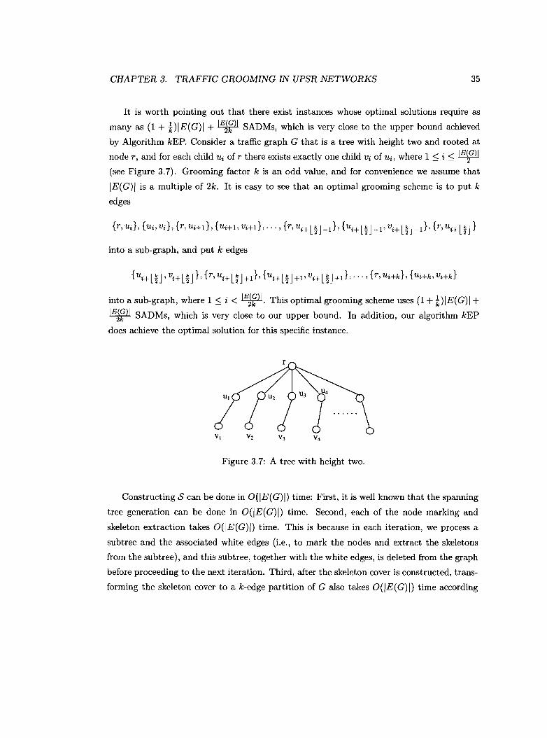
CHAPTER 3. TRAFFIC GROOMING IN UPSR NETWORKS 35
It is worth pointing out that there exist instances whose optimal solutions require as
many as (1 + i)IE(G)1 + IEJfll SADMs, which is very close to the upper bound achieved
by Algorithm kEP. Consider a traffic graph G that is a tree with height two and rooted at
node r, and for each child Ui of r there exists exactly one child Vi of Ui, where 1 ~ i ~ IE~Gll
(see Figure 3.7). Grooming factor k is an odd value, and for convenience we assume that
IE(G)/ is a multiple of 2k. It is easy to see that an optimal grooming scheme is to put k
edges
into a sub-graph, and put kedges
{UH l~J' vHl~J}' {r, uHl~J+1}' {uHl~J+1' Vi+ l~J +1}' ... ,{r, UHk}, {UHk, Vi+k}
into a sub-graph, where 1 ~ i < IEJfll. This optimal grooming scheme uses (1 + !)IE(G)j +IEJ~ll SADMs, which is very close to our upper bound. In addition, our algorithm kEP
does achieve the optimal solution for this specific instance.
Figure 3.7: A tree with height two.
Constructing S can be done in O(IE(G)I) time: First, it is well known that the spanning
tree generation can be done in O(IE(G)I) time. Second, each of the node marking and
skeleton extraction takes O(IE(G)I) time. This is because in each iteration, we process a
subtree and the associated white edges (Le., to mark the nodes and extract the skeletons
from the subtree), and this subtree, together with the white edges, is deleted from the graph
before proceeding to the next iteration. Third, after the skeleton cover is constructed, trans
forming the skeleton cover to a k-edge partition of G also takes O(IE(G)I) time according
CHAPTER 3. TRAFFIC GROOMING IN UPSR NETWORKS 36
to Proposition 3. Therefore, Algorithm kEP runs in O(IE(G)I) time, which is linear in the
size of the input graph.
Goldschmidt et al. [28] established a lower bound by observing that each sub-graph in
the best possible k-edge partition is a complete graph with exactly k edges. Therefore, the
total number of nodes over all sub-graphs is bounded below by IE~G)I . 1+/fB. Based on
this lower bound, we have the following theorem for Algorithm kEP.
Theorem 8 For a graph G with m edges and n nodes, and an integer k, Algorithm kEP is
a~(r(l + k)ml + l~J)
1+y'8ffi2
approximation algorithm for the k-Edge-Partitioning problem.
Proof: Trivial.
3.2.3 Algorithm SpanT...Euler
o
The k-Edge-Partitioning algorithms that we have discussed so far fall into two categories:
spanning-tree based algorithms(the algorithm in [28] and Algorithm kEP) and Euler-path
based algorithm (the algorithm in [11]). In this section, we propose a linear time approx
imation algorithm SpanT-Euler, which combines the spanning-tree based skeleton cover
approach used by Algorithm kEP and the Euler-path based approach used in [11]. Algo
rithm SpanT_Euler tries to minimize the total number of components over all sub-graphs as
well, and achieves an upper bound that is at least as good as the one obtained by Algorithm
kEP. Algorithm SpanT-Euler also uses the minimum number r'E~G)'l of wavelengths.
The algorithm
In order to achieve good solutions for the k-Edge-Partitioning problem, the obtained k-edge
partition should contain as few components as possible over all sub-graphs. The algorithm
in [11] constructs an Euler path of traffic graph G by adding virtual edges between odd
degree nodes. Then the Euler path is cut into segments and virtual edges are deleted to
obtain a k-edge partition of G. However in the case that G contains a large number of
odd-degree nodes, there will be a large number of virtual edges, whose deletion further
implies a large number of components over sub-graphs in the k-edge partition. Algorithm
CHAPTER 3. TRAFFIC GROOMING IN UPSR NETWORKS 37
kEP constructs a skeleton cover of G, and then transform the skeleton cover into a k-edge
partition. Skeleton are constructed using a spanning-tree based approach, which likely
produces skeletons with small size, and thus the size of the skeleton cover is usually large.
According to Proposition 3, a skeleton cover with large size yields a solution of the k-Edge
Partitioning problem with large value. In this section, we propose Algorithm SpanT_Euler
that combines the techniques of constructing the Euler path and the skeleton cover. We
intend to generate a skeleton cover of small size with the help of Euler path construction.
On constructing a skeleton cover, the following lemma holds.
Lemma 9 If there exist l edge-disjoint paths which span every node in graph G, then G has
a skeleton cover with size l.
Proof: Each of the l paths can be considered as the backbone of a skeleton. Since the
backbones span every node in graph G, other edges which do not appear in the backbones
can be attached as branches. Thus the size of the constructed skeleton cover is exactly I. 0
It is proved by Jaeger [36] that if the edge connectivity of G is at least four, then there
exists a path that spans every node in G, which implies that there exists a skeleton cover
with size one for graph G according to Lemma 9. Following a similar argument, we generalize
the result of [36] as the following Lemma.
Lemma 10 Let T be a spanning tree of G, and c be the number of components in graph
G(V(G),E(G)\E(T», then G has a skeleton cover with size at most c.
Proof: Let Vodd ~ V(G) be the set of nodes having odd degree in graph G(V(G), E(G)\E(T».
lVoddl must be even since the number of odd-degree nodes in any graph is even. Pair the
nodes of Vodd arbitrarily and let P = {pl,p2,'" ,PJ.Y..wtl} be the set of simple paths in T2
between each pair of nodes. For every edge e E E(T), let a(e) denote the number of paths
(in P) that contain edge e. Define
Eodd = {ele E E(T) and a(e) is odd}, and
Eeven = {ele E E(T),a(e) is even, and a(e) =I- OJ.
We prove in the following that Vodd is also the set of nodes that have odd degree in graph
G(V(G), Eodd)'
CHAPTER 3. TRAFFIC GROOMING IN UPSR NETWORKS 38
For every node v E Vodd, let Ev ~ Eodd U Eeven be the set of edges adjacent to node v.
We notice that v is an end-node for exactly one path in P (i.e., only one edge in the path
is adjacent to v), and for any other path in P, either v is a mid-node of the path (i.e., two
edges in the path are adjacent to v) or v is not in the path (i.e., no edge in the path is
adjacent to v). Therefore l:eEEv a(e) must be odd. We also know that
L a(e) = L a(e) + L a(e),eEEv eE(EvnEodd) eE(EvnEeven)
so jEvnEoddl must be odd, that is, every node v E Vodd has odd degree in graph G(V(G), Eodd)'
Similarly for every node u E V(G)\Vodd , since either u is a mid-node of some paths or u is
not in any path, we have that l:eEEu a(e) must be even. That is,
L a(e) = L a(e) + L a(e)eEEu eE(EunEodd) eE(EunEeve,,)
must be even, and thus lEu n Eoddl must be even. Therefore every node u E V(G)\Vodd has
even degree in graph G(V(G), Eodd).
Since Vodd is defined to be the set of nodes having odd degree in graph G(V(G), E(G)\E(T)),
every node in graph G' = G(V(G), Eodd U (E(G)\E(T))) has even degree. We know that
G(V(G), E(G)\E(T)) contains at most c components, so there are at most c components
in graph G' as well. For each component in graph G', we can construct an Euler path since
all nodes have even degree (for the component consisting of a single node, the Euler path
is a special one consisting of the single node). It is clear that the Euler paths span every
node in G. Thus we can construct a skeleton cover of G with size at most c according to
Lemma 9. 0
Notice that a component of graph G' contains either a single node or at least three nodes
since each node has an even degree. A component is called small if it contains at most three
nodes, otherwise called large. In the worst case, the size c of the skeleton cover constructed
above could be as large as the number n of nodes in graph G (in this case, graph G is a tree
T and removing the edges of T gives c = n components, each of which is small component
containing a single node). To further bound the size of the skeleton cover, we use Algorithm
kEP to handle the small components of graph G'.
Given a graph G and a spanning tree T, let H be the sub-graph of G induced by the
nodes of the small components of G'. For a component h of H, there is an edge {u, v} and a
large component 9 of G' such that u E V(h) and v E V(g), since graph G is connected. We
CHAPTER 3. TRAFFIC GROOMING IN UPSR NETWORKS 39
select one such 9 and edge {u, v} for h. If h has at most three nodes, then we connect h to
9 via edge {u, v} as an attachment. Otherwise, we use Algorithm kEP to extract skeletons
from h with node u as the root of the spanning tree of h until at most three nodes are left
in h, and let hi be the remaining sub-graph of h. We connect hi to 9 via edge {u, v} as an
attachment. Notice that hi is a path u - x - y of three nodes and nodes x and y do not appear
in any previously extracted skeletons (Le., nodes x and y can be treated as characteristic
nodes when they are included into some skeleton later). According to the above description,
an attachment must be one of the following five cases: a single node, a I-path, two I-paths,
a 2-path, or a triangle (see Figure 3.8(a)). We call an attachment large if it has at least
two nodes, and small if it is a single node. Obviously, a large attachment contains at least
two nodes which can be treated as characteristic nodes when they are included into some
skeleton later. For each large attachment, we select a longest path from v to a node in the
attachment as the main-path of the attachment (see Figure 3.8(a)).
For every large component 9 of G' , we find an Euler cycle of g. For every node v in
g, if there are at least two large attachments connected to v then we extract a skeleton
with the backbone to be the main-paths of two large attachments. There are at least four
characteristic nodes in the skeleton. We repeat this procedure until at most one large
attachment is connected to v. After the process, we have an Euler cycle of 9 and each node
v in the cycle is connected to at most one large attachment.
We view the Euler cycle of 9 as a ring with IE(g)1 edges (see Figure 3.8(b)). A node
v of 9 may appear multiple times in the ring. We arbitrarily select one appearance as the
real v and call any other a copy of v. All attachments connected to v are connected to the
real v in the ring. We call node v in the ring a special node if it is connected .to one large
attachment. The extraction of skeletons for large component 9 are now divided into the
following several cases:
• Case 1: there is no special node in the ring. A single skeleton is extracted with
the backbone as an Euler path of g, and any small attachment connected to 9 can
be treated as a branch (in the following, we will only mention the backbone of each
skeleton, since once the backbone is obtained, it is easy to decide the corresponding
branches). Notice that the backbone contains at least four nodes which do not appear
in any other skeleton, and thus can be treated as characteristic nodes.
• Case 2: there is one special node v in the ring. A single skeleton is extracted with
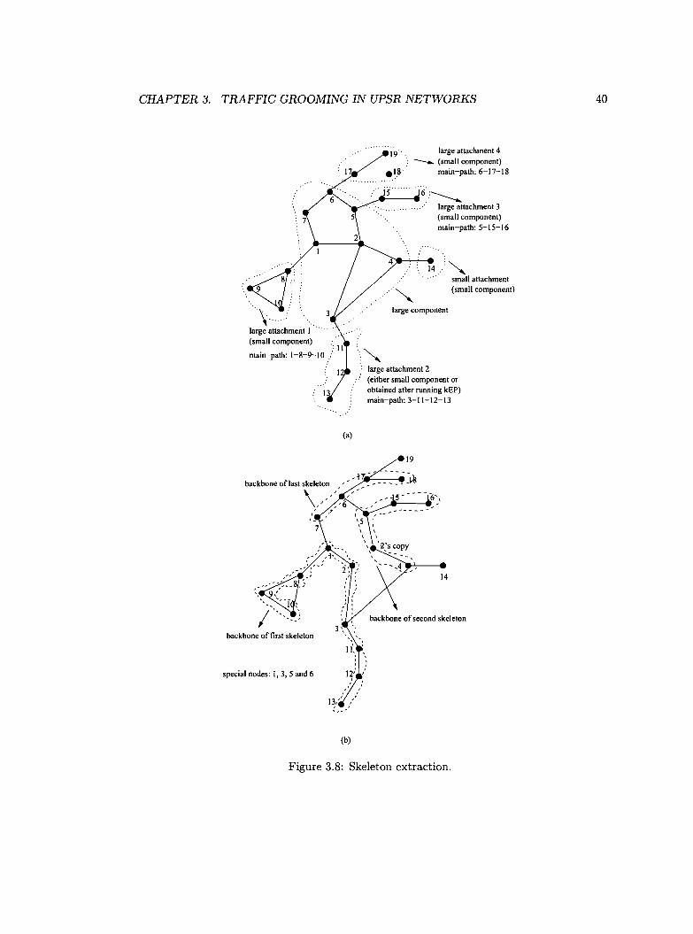
CHAPTER 3. TRAFFIC GROOMING IN UPSR NETWORKS 40
'iC}
:'. 1,~F--_1S
large attachment 4--... (small component)
main-path: 6-17-18
large component
large attachment 2(either small component orobtained after running kEP)main-path: 3-11-12-13
~small attachment(small component).,~
~ 16:______
large attachment 3(small component)main-path: 5-15-16
\ ..large attachment 1(small component)
main-path: 1-8-9--10
(a)
19
14
backbone of second skeleton
backbone oflas! skeleton " - - t~ ~ ~ - .'~ .' .' --~
\"<'6," .'
backbone of first skeleton
special nodes: I, 3, 5 and 6
(b)
Figure 3.8: Skeleton extraction.
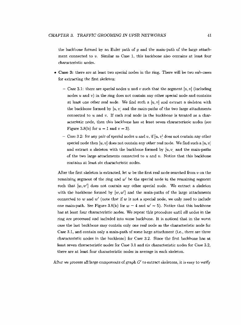
CHAPTER 3. TRAFFIC GROOMING IN UPSR NETWORKS 41
the backbone formed by an Euler path of 9 and the main-path of the large attach
ment connected to v. Similar as Case 1, this backbone also contains at least four
characteristic nodes.
• Case 3: there are at least two special nodes in the ring. There will be two sub-cases
for extracting the first skeleton:
- Case 3.1: there are special nodes u and v such that the segment [u, v] (including
nodes u and v) in the ring does not contain any other special node and contains
at least one other real node. We find such a [u, v] and extract a skeleton with
the backbone formed by [u, v] and the main-paths of the two large attachments
connected to u and v. If each real node in the backbone is treated as a char
acteristic node, then this backbone has at least seven characteristic nodes (see
Figure 3.8(b) for u = 1 and v = 3).
- Case 3.2: for any pair of special nodes u and v, if [u, v] does not contain any other
special node then [u, v] does not contain any other real node. We find such a [u, v]
and extract a skeleton with the backbone formed by [u, v] and the main-paths
of the two large attachments connected to u and v. Notice that this backbone
contains at least six characteristic nodes.
After the first skeleton is extracted, let W be the first real node searched from v on the
remaining segment of the ring and Wi be the special node in the remaining segment
such that [w, Wi] does not contain any other special node. We extract a skeleton
with the backbone formed by [w, Wi] and the main-paths of the large attachments
connected to wand Wi (note that if w is not a special node, we only need to include
one main-path. See Figure 3.8(b) for w = 4 and Wi = 5). Notice that this backbone
has at least four characteristic nodes. We repeat this procedure until all nodes in the
ring are processed and included into some backbone. It is noticed that in the worst
case the last backbone may contain only one real node as the characteristic node for
Case 3.1, and contain only a main-path of some large attachment (i.e., there are three
characteristic nodes in the backbone) for Case 3.2. Since the first backbone has at
least seven characteristic nodes for Case 3.1 and six characteristic nodes for Case 3.2,
there are at least four characteristic nodes in average in each skeleton.
After we process all large components of graph GI to extract skeletons, it is easy to verify
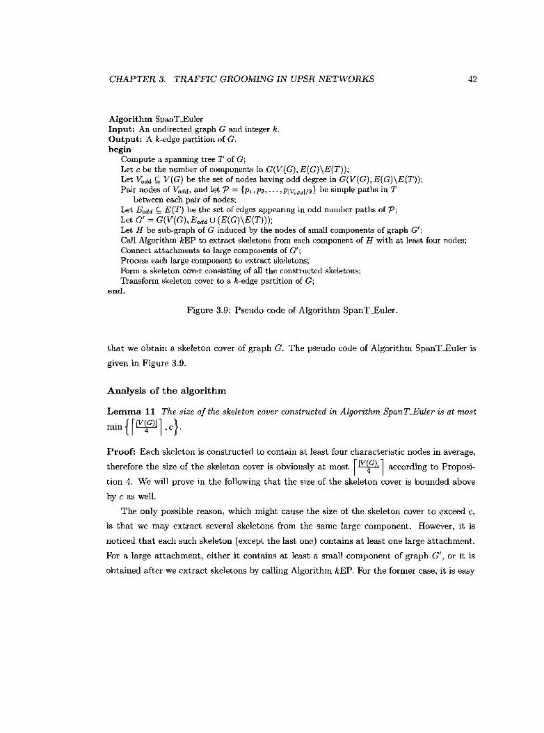
CHAPTER 3. TRAFFIC GROOMING IN UPSR NETWORKS
Algorithm SpanT..EulerInput: An undirected graph G and integer k.Output: A k-edge partition of G.begin
Compute a spanning tree T of G;Let c be the number of components in G(V(G), E(G)\E(T));Let Vodd ~ V(G) be the set of nodes having odd degree in G(V(G), E(G)\E(T));Pair nodes of Vodd , and let P = {PI, P2, ... ,PlVoddl/2} be simple paths in T
between each pair of nodes;Let Eodd ~ E(T) be the set of edges appearing in odd number paths of P;Let G' = G(V(G), E odd U (E(G)\E(T)));Let H be sub-graph of G induced by the nodes of small components of graph G';Call Algorithm kEP to extract skeletons from each component of H with at least four nodes;Connect attachments to large components of G';Process each large component to extract skeletons;Form a skeleton cover consisting of all the constructed skeletons;Transform skeleton cover to a k-edge partition of G;
end.
Figure 3.9: Pseudo code of Algorithm SpanT_Euler.
42
that we obtain a skeleton cover of graph G. The pseudo code of Algorithm SpanT-Euler is
given in Figure 3.9.
Analysis of the algorithm
Lemma 11 The size of the skeleton cover constructed in Algorithm Span T.Euler is at most
minH~l ,e}.Proof: Each skeleton is constructed to contain at least four characteristic nodes in average,
therefore the size of the skeleton cover is obviously at most rIV~G)'1 according to Proposi
tion 4. We will prove in the following that the size of the skeleton cover is bounded above
bye as well.
The only possible reason, which might cause the size of the skeleton cover to exceed e,
is that we may extract several skeletons from the same large component. However, it is
noticed that each such skeleton (except the last one) contains at least one large attachment.
For a large attachment, either it contains at least a small component of graph G', or it is
obtained after we extract skeletons by calling Algorithm kEP. For the former case, it is easy
CHAPTER 3. TRAFFIC GROOMING IN UPSR NETWORKS 43
to conclude that cutting a large component into skeletons will not make the number of con
structed skeletons exceed c, since each such skeleton contains at least one small component
of G'. For the latter case, the large attachment is obtained after extracting skeletons from
some component h of H (recall that H is the sub-graph of G induced by the nodes of the
small components of G'). We also know that each such extracted skeleton contains at least
four characteristic nodes, and h is composed of small components containing at most three
nodes. Therefore, the number of extracted skeletons from h must be at least one less than
the number of small components contained in h. Therefore, we can have the same conclusion
as the former case. In summary, we conclude that the total number of constructed skeletons
in Algorithm SpanT-.Euler can not exceed c. 0
Theorem 12 Algorithm SpanT_Euler finds a k-edge partition [; = {E1, ... , Ew } of G with
W = fIE1G)'lIEil = k for 1:::; i < W, and
EE;E£ IViI :::; f(1 + k)IE(G)1l + min {llV~G)IJ ,(c - I)}.
Proof: The theorem can be easily proved based on Proposition 3 and Lemma 11. 0
By Theorem 12, at most f(1 + k)IE(G)il +min {llV\G)IJ ' (c - I)} SADMs are used by
Algorithm SpanT-.Euler. It is also noticed that the algorithm uses the minimum number
f'E1G)'l of wavelengths for a traffic graph G.
Similarly, we have the following theorem for Algorithm SpanT_Euler.
Theorem 13 For a graph G with m edges and n nodes, and an integer k, Algorithm
SpanT_Euler is a~(f(1 + k)ml + l~J)
1+v'8k±12
approximation algorithm for the k-Edge-Partitioning problem.
Proof: Trivial. D.
Since the spanning tree generation and Euler path construction can be done in O(jE(G)I)
time, it is clear that each step of Algorithm SpanT_Euler takes O(IE(G)I) time. So Algo
rithm SpanT-.Euler runs in O(IE(G)/) time, which is linear in the size of the input graph.
3.3 Empirical results
In this section, we will conduct extensive simulations to evaluate the practical performances
of our algorithms by comparing to existing algorithms. We implemented the algorithms
CHAPTER 3. TRAFFIC GROOMING IN UPSR NETWORKS 44
in [11, 28], our approximation algorithms kEP and SpanT_Euler to compare their perfor
mances on randomly generated traffic graphs. In generating graphs, we specify the number
n of nodes and density ratio d that is used to calculate the number m = n 1+d of edges.
A graph of m edges and n nodes is generated by randomly connecting m pairs of nodes
among all n(n - 1)/2 possible pairs. We refer to the algorithms in [28J anq [l1J as Algo.
1 and Algo. 2 respectively. Figure 3.10 shows the empirical results for graphs of 36 nodes
with different settings of density ratio d and grooming factor k. For each pair of values
of d and k, we run the algorithms on 100 randomly generated traffic graphs and take the
average number of required SADMs. We observe that the spanning-tree based Algo. 1 and
Algo. kEP have better performances if density ratio d is smaller, and the Euler-path based
Algo. 2 has better performance if density ratio d is larger. As we pointed out previously,
Algorithm SpanT_Euler combines the techniques of constructing Euler path and skeleton
cover. Therefore, Algorithm SpanT_Euler can be considered as a hybrid of the spanning-tree
based approach and the Euler-path based approach. The empirical results in Figure 3.10
verify that Algorithm SpanT-Euler does take advantages of both approaches, and has bet
ter performance than all of the previous algorithms. Also, we would like to mention that
for Algorithm SpanT_Euler and confidence interval [1 - 5%,1 + 5%], the confidence lev
els are 88%,93%,96%,98%,99% and 100% for density ratio d = 0.1,0.2,0.3,0.4,0.5 and 0.6
respectively. We ran simulations on graphs with different parameter settings as well, and
the results present similar characteristics (see Figure 3.11 and Figure 3.12 for some other
representative results).
3.4 Summary
In this chapter, we proposed two linear time approximation algorithms for the traffic groom
ing problem in the SONET/WDM UPSR network with unitary duplex traffic demands. Our
algorithms achieve better upper bounds on the number of SADMs and experimental per
formances compared to previous ones, and they use the minimum number of wavelengths,
which are also precious resources in optical networks. The gap between the upper bounds of
our algorithms and the lower bound for arbitrary traffic graphs is still large (see Theorem 8
and Theorem 13). An interesting open problem is to further narrow the gap. The problem
seems challenging for arbitrary graphs because the upper bounds of our algorithms have
been shown very close to the optima for some sparse graph instances. The difficulty in
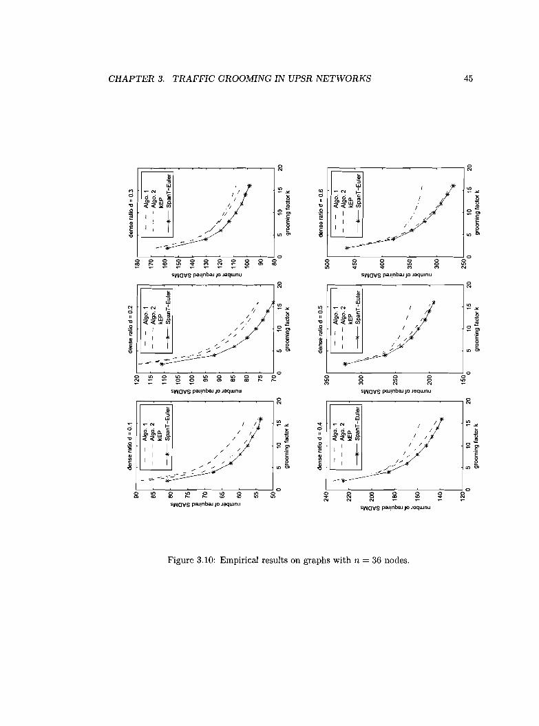
CHAPTER 3. TRAFFIC GROOMING IN UPSR NETWORKS 45
0 0N N
Ii; Ii;'3 '3UJ
II)UJ I II)
M ~NI
~ ~NI
l- i I ~ .>< I- ~ .><0 .. c:
~0 .. c:
I ~II o 0 a. m I II o 0 a. m'0
OJ .QJ UJ c.II '0
,2J .QJ UJ c.<<(.><Ul .. ««.><Ul ,; ..
~ I t II0- 0
t0-
~ g'~
~ g'., I / 'E .,
'"'E
'" /0 '" I
~c: I e c:., .,'0 II) Cl '0 II) Cl
0 00 0 0 0 0 0 0 0 0 al 0 0 0 0 0 0 0
~ .... ~II) '" ~
N~ co 0 II) 0 II) 0 II)
II) '" '" M M N
SVOlavs paJ!nbaJ /0 Jaqwnu SVOlavs paJ!nbaJ /0 Jaqwnu
0 0N N
Ii; Ii;'3 '3UJ
II)UJ
II)N ~ N I II) ~ N I
0 l- I; ~ .><0 I- ~ .><
.. c:
~ OOo..~ (;II ~~fu~ I II .QJ .QJ LLJ a. I ()'0 ««.><Ul // .. '0 ««.><Ul ...2 J
t/ I 0- 0
tI. 0-
'@ ~ g' "" ~ g'// ~ I., I
",-"'E ., // 'E
'" 0 '" 0c: I "', e c: I A e., , ., ,'0 , II) Cl '0 II) Cl
_...-- -0 0
0 II)~
II) 0 II) 0 II) 0 II) 0 0 0 0 0 0
~ ;:: ~ ~m m CO CO .... .... II) 0 II) 0 II)
M M N N
SVOlaVS paJ!nbaJ /0 Jaqwnu SVOlaVS p9J!nbaJ /0 Jaqwnu
0 0N N
Ii; Ii;'3 '3w
II)UJ
II)~N
I I "': ~NI I
0 I- ~ .>< l- I ~ .><o 0 a. f6 ~
0 .. c:I
~II I II o 0 a. to.,!2)OJ W C. OJ .QJ UJ a. I
'0 «<.><Ul / .. '0 <<(.><Ul I ..0
t/
I 0- 0
tI / 0-
"" I ~ g'~
I ~ g'l!! / /., I /
'E III I I", E'" ° 0c: I '" e c: I /'" e.,
II) Cl.,
II) Cl'0 '0
0 00 II) 0 II) 0 II) 0 II) 0 0 0 8 0 0 0 0m CO CO .... .... CD CD II) II) '" N
~ ~ ~ ~N N NSVOlaVS paJ!nbaJ /0 Jaqwnu
SVOlaVS paJ!nbaJ /0 Jaqwnu
Figure 3.10: Empirical results on graphs with n = 36 nodes.
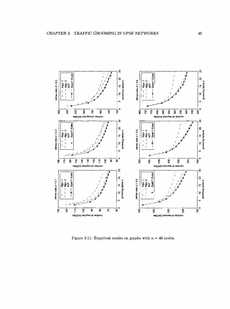
CHAPTER 3. TRAFFIC GROOMING IN UPSR NETWORKS 46
It) It)N N
jj I lii:> I I 0
:;0w W
M ~ N II I
NCD I I N
0 I- 0~ N I-
o 0 a.. ~ <; o ci a.. ~ <;" .Q) en LU 0. I I
~U " .Q) ,Q) UJ 0- J~o'0 <C<.><CI> . I :: '0 ««~(I) ::0
I
fII '" ~ J
t '"..e c: c:Ql I 1/ ~ 'E Ql I I ~ 'E<II /' 0 <II 0c: I e c: I I eQl / '"
Ql
'"'0 / '0 .-,- It) It)
0 00 0 0 0 0 0 0 0 0 0 0 0 0 0 0 0 0 0 0CD .. N 0 e:' ~ ~ ~
0 It) 0 It) 0 It) 0 It) 0 It) 0N N N N co ... ... CD CD It) It) .. .. M M
S~a\fS p,,,!nb9J 10 J9qwnu s~a\fS p9J!nb9J 10 J9qwnuIt) It)N N
lii,
jj:; {
0:>
0W ( WN I N
It) I N~ N l- ) .>< ~N I- .><
0 " c: <; 0 o ci a.. ~ l5" o 0 a.. co "'0.Q>.Q) LU a. II It)U
'0.Q> .Q> UJ 0- It)u<C<C.><CI> ~:: <C<C.><CI> ~::
0 I
rII '"
0I
t '"'e ..II '~ e c:
Ql I ~ Ql I ~ ·E<II /. 0 <II 0c: I II e c: I eQl
'"Ql
'"'0 // '0/,..- It) It)
---0 0
0 0 0 0 0 0 0 0 0 0 0 0 g 0 0 0 0 0
e:' ...~
It)~
M N 0 a> co It) It) 0 It) 0 It)It) It) .. .. M M N
S~a\fS p9J!nb9J 10 J9qwnu S~a\fS p9J!nb9J 10 J9qwnuIt) It)N N
lii I liiI:; :;
w I 0 w 0I N
": I IN
0~ N l- I .>< ~N I-,. c:
l5 0 o d a.. li <;"
o 00.. co" IjJ)tnUJQ. I It)U .Q>.Q>wa. It)U
'0 <C<.><CI> ~:: '0 <C<C.><CI> ~::
~ I
tI
'" ~ I
~I
'"I c: c:
5l I I I ~ 'E Ql I 1/ ~ E0 <II
I0
c: I I I e c: I II eQl
'"Ql
// '"'0 '0
/It) A It)
"'-"'-_,c;::;:.
0 00 0 0 0 0 0 0 0 0 0 0 0 0M
~ ~a> CO ... CD It) 0 It) 0
~M M N N
S~a\fS p9J!nb9.J 10 J9qwnu s~a\fS p9J!nb9J 10 J9qwnu
Figure 3.11: Empirical results on graphs with n = 48 nodes.
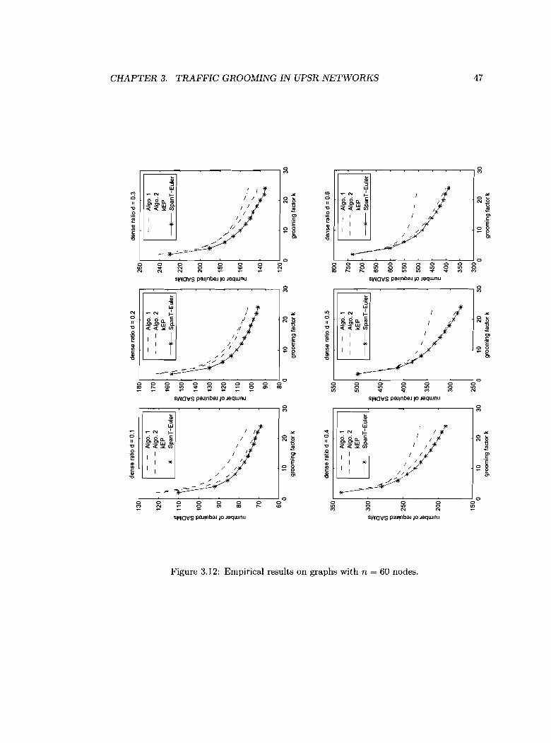
CHAPTER 3. TRAFFIC GROOMING IN UPSR NETWORKS 47
CDc:i
""0o~5l16"0
II I
I I, I
i lII
,,;./
-'--:
Mc:i
""0o~
'".,~
oL----o~----,~--=o,-----o=---=o,-----o=----:'o a~ ~ ~ w W V N
O~---'=----::----='-----=:---=i5'----O=----'O=----'O=----:O:------:Oa~ ~ g ~ ~ ~ g
S!'lOI7'S pOJ!nboJ )0 Joqwnu S!'lOI7'S pOJ!nbaJ )0 Joqwnu
L------=,------..,__~__~--_=_-____::O
~ ~ g ~S!'lOI7'S pOJ!nbaJ )0 Jaqwnu
It)
c:i
""0o~
'".,16"0
(I
"IIII/,
I I/1
//// .
'":;W
,.....N ~.. "o 0 Q. to
99UJ a.«.><(/)
: t
S!'lOI7'S pOJ!nboJ)o Jaqwnu
Nc:i
""0
,gt!!
'".,~
r;:::====::;---~--~--IgI;;:;w
.... N ~
ci ci Q. ~
~~~c%
: t
L-----~---,----i5~----g~---....Ji5aN N
"':a
""0
gt!!
'".,"'""0
I II
I
II
/
/
M0L----O~--~--=,----~--,.O,-----,O=--....JOa
N w ~ w
c:i
""0
,gt!!
'".,~"0
S!'lOI7'S pOJ!nboJ )0 Joqwnu S!'lOI7'S paJ!nboJ )0 Jaqwnu
Figure 3.12: Empirical results on graphs with n = 60 nodes.
CHAPTER 3. TRAFFIC GROOMING IN UPSR NETWORKS 48
narrowing the gap is that sparse graphs (e.g., trees) are shown the barriers for improving
the upper bounds, while the lower bound is based on the assumption that the graph can be
partitioned into cliques, which implies the graph is either dense or has a special structure.
One possible approach is to develop different lower bounds and algorithms for graphs with
different densities. For dense graphs, it is interesting to design algorithms which partition
the traffic graph into dense subgraphs, each of which is a clique or close to a clique. For
sparse graphs, a better lower bound seems necessary.
Chapter 4
Traffic grooming in UPSR with
regular traffic
In this chapter, we study the regular traffic pattern, which is considered as a generalization
of the well-known all-to-all traffic pattern. We focus on the Unidirectional Path-Switched
Ring (UPSR) networks as well. We prove that the traffic grooming problem is NP-hard for
the regular traffic pattern in UPSR networks, and show that the problem does not admit
a Fully Polynomial Time Approximation Scheme (FPTAS) unless P = N P. We further
prove that the problem remains NP-hard even if the grooming factor is any value chosen
from a subset of integers. We also propose a performance guaranteed algorithm to minimize
the total number of required SADMs, and show that the algorithm achieves a better upper
bound on the number of SADMs than previous algorithms applying on the regular traffic
pattern. In addition, our algorithm always uses the minimum number of wavelengths, which
are precious resources as well in optical networks.
4.1 Problem formulation
Recall that the traffic grooming problem in UPSR networks with duplex traffic pattern can
be formulated as the k-Edge-Partitioning problem on the traffic graph. In this chapter, we
study the regular traffic pattern, in which each network node is involved in r duplex traffic
demand pairs in the network, where 1 ::; r ::; n -1 for a network of n nodes. For the regular
traffic pattern, the traffic graph is a regular graph, and the traffic grooming problem can be
49
CHAPTER 4. TRAFFIC GROOMING IN UPSR WITH REGULAR TRAFFIC 50
formulated as the following k-Edge-Partitioning of Regular Graph problem:
k-Edge-Partitioning of Regular Graph Problem
Instance: A regular traffic graph G(V, E) and integer k ~ IE(G)I.
Objective: Partition the edge set E(G) into a collection of subsets [; = {Ell E2,···, Ew}
(where U~lEi = E(G) and Ep n Eq = 0 for p -I- q), such that IEil ~ k for each E i E [; and
l:EiE£IViI is minimized, where Vi is the set of nodes in the sub-graph induced by edge set
Ei.
The regular traffic pattern is a generalization of the well known all-to-all traffic pattern,
for which the traffic grooming problem has been well studied in [7, 32, 42, 64J. The regular
traffic pattern is of high practical interest, since optical network nodes usually have limited
capacity on sourcing/ending traffic demands simultaneously at any time due to the hard
ware constraints. To the best of our knowledge, this is the first time that the regular traffic
grooming problem is addressed. It has been shown that the k-Edge-Partitioning problem
on arbitrary traffic graphs is NP-hard [28J. We prove that the k-Edge-Partitioning of Reg
ular Graph problem remains NP-hard, and show that the problem does not admit a Fully
Polynomial Time Approximation Scheme (FPTAS) unless P = N P. As well, we prove the
problem remains NP-hard even if k = a(a - 1)/2 for each integer a 2: 3. We also propose
a performance guaranteed algorithm that achieves a better upper bound than previous al
gorithms designed for general duplex traffic patterns. In addition, our algorithm uses the
minimum number of wavelengths, which are precious resources as well in SONET/WDM
networks. We also conduct extensive simulations to evaluate the average performance of
our algorithm.
4.2 Computational complexity
In this section we analyze the computational complexity of the k-Edge-Partitioning problem
on regular graphs. We first prove that the k-Edge-Partitioning problem is NP-hard on r
regular graph for an arbitrary value of r, and further prove that the problem does not admit
an FPTAS unless P = N P. In addition, we show that the problem remains NP-hard even
if k = a(a - 1)/2, where a 2: 3 is integer and k < IE(G)I.
CHAPTER 4. TRAFFIC GROOMING IN UPSR WITH REGULAR TRAFFIC 51
4.2.1 NP-hardness
We consider the decision version of the k-Edge-Partitioning of Regular Graph (kEPRG)
problem, and prove it is NP-complete. The kEPRG problem is stated as follows:
k-Edge-Partitioning of Regular Graph (kEPRG) Problem
Instance: An undirected regular graph G(V, E), and integers k and T.
Question: Is there a partition of E(G) into a collection of subsets £ = {El , E 2, ... , Ew}
(where U:lEi = E(G) and Ep n Eq = 0 for Pi- q), such that lEi! ::; k for each Ei E £ and
LEiE£IViI ::; T, where Vi is the set of nodes in the sub-graph induced by edge set E i ?
We give a two-step reduction from the Edge-Partition into Triangles (EPT) problem to
the kEPRG problem. The EPT problem is known to be NP-complete [31] and stated as
follows:
Edge-Partition into Triangles (EPT) Problem
Instance: An undirected graph G(V, E) with IE(G)I = m.
Question: Is there a partition of E(G) into sets {El , E2, ... , E m / 3 } such that each Ei induces
a triangle?
In the first step we show that the EPT problem on regular graphs is NP-complete by a
reduction from the EPT problem.
Lemma 14 The EPT problem remains NP-complete when the input graph G is regular.
Proof: It is easy to see that if an odd-degree node exists in a graph, the graph can not be
partitioned into triangles. Therefore, the EPT problem is NP-complete even if the input
graph contains no odd-degree nodes. Otherwise, the EPT problem itself is not NP-complete.
In what follows, we assume the input graph has no odd-degree nodes when we refer to an
instance of the EPT problem.
The regular graph version of EPT is clearly in NP. Given an undirected graph G with
maximum degree ~ (where ~ is even) , we construct a ~-regular graph G* as follows (for
simplicity, we use (u,v,w) to denote a triangle with {u,v,w} as node set):
1. For every node v in G with degree 8(v) < ~, add triangles {(V,Uv,i,Uv,i+I)} for
i = 1,3,5, ... ,~ - 8(v) - 1 to get graph G' , where the ~ - 8(v) nodes uv,i's and
Uv,i+l'S are the new added nodes.
2. Make two extra copies of G' , and assume the number of new added nodes in G' is q.
CHAPTER 4. TRAFFIC GROOMING IN UPSR WITH REGULAR TRAFFIC 52
3. Re-Iabel all the new added nodes as UI, U2, U3, ... , U3q'
4. If 3q < ~22
(a) add 3p new nodes U3q+I, U3q+2, U3q+3, ... , U3q+3p, where p is the smallest integer
satisfying 3q + 3p 2: ~22;
(b) add p triangles {(U3q+i, U3q+i+1, U3q+i+2)} for i = 1,4,7, ... , 3p - 2;
(c) set q = q + p.
5. Add 3q new nodes WI,W2, W3, ... ,W3q and q triangles {(Wi, Wi+I, Wi+2)} fori = 1,4,7, ... , 3q
2. Add another 3q new nodes YI,Y2,Y3, ... ,Y3q and q triangles {(Yi,Yi+I,Yi+2)} for
i = 1,4,7, ... , 3q - 2.
6. Repeat the following for i = 1,2,3, ... , ~22: add triangles {(Uj, WjEBi, YjEB2i)} for j =1,2,3, ... ,3q, where EB is defined as mod 3q sum.
It is easy to verify that graph G* constructed above is a b.-regular graph. Figure 4.1
illustrates an example to construct regular graph G* based on the given graph G (we make
two copies for nodes YI, Y2 and WI to avoid messy drawing).
Now we prove that G can be partitioned into triangles if and only if G* can be partitioned
into triangles. If G can be partitioned into triangles, according to the construction of G*, G*
can be partitioned into triangles as well. If G* can be partitioned into triangles, it is noticed
that any triangle containing an edge from a copy of G can not contain any edge outside of
that copy. So each copy of G by itself must be able to be partitioned into triangles. 0
In the second step we show that the kEPRG problem is NP-complete by a reduction
from the regular graph version of the EPT problem.
Theorem 15 The kEPRG problem is NP-complete.
Proof: The problem is clearly in NP. Given an instance of the regular graph version of
EPT problem, where the input graph G is regular, we construct an instance of the kEPRG
problem on the same graph with T = m and k = 3, where m = IE(G)I.
If G can be partitioned into triangles, the triangle partition gives a solution for the
kEPRG problem where IEil = 3 for each E i E £ and LEiEt: IYiI = m.
We now prove that if G has a solution for the kEPRG problem with k = 3 and T = m,
then it can be partitioned into triangles. It is noticed that LEiEt: IYiI 2: m for k = 3, and the
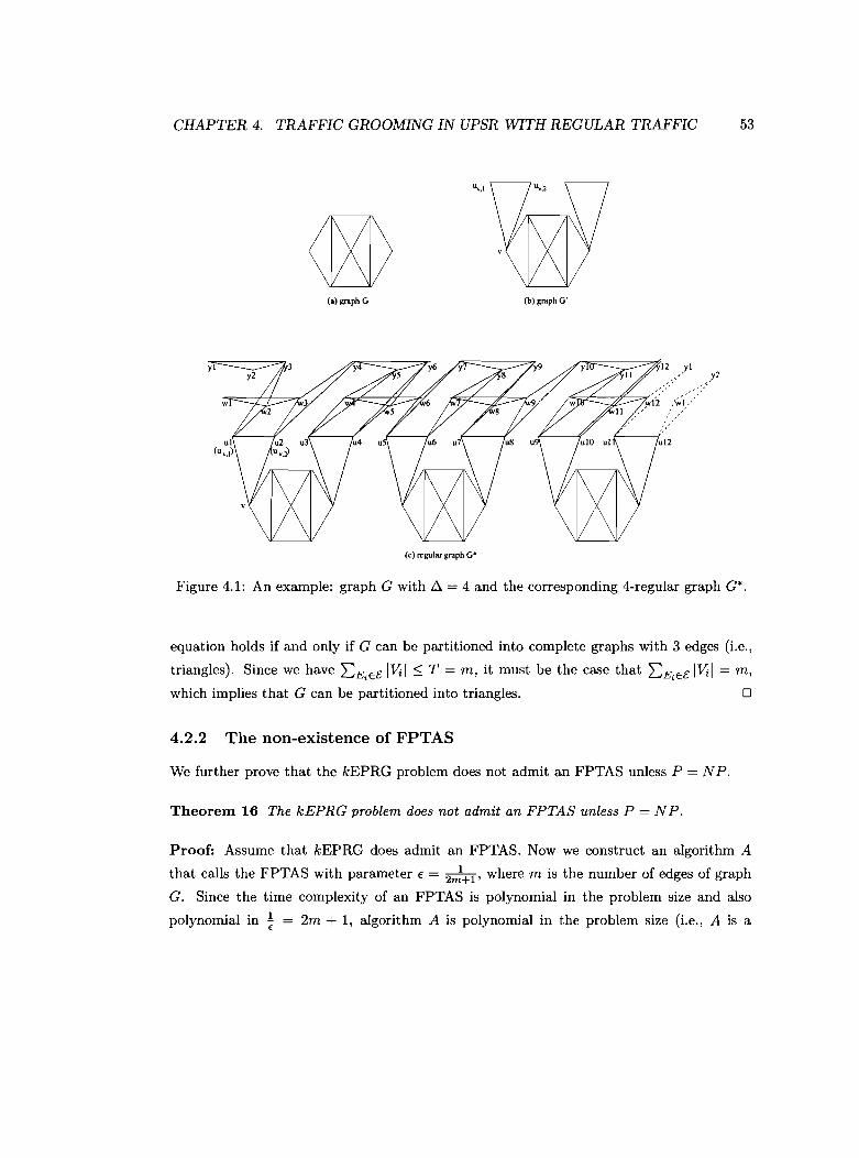
CHAPTER 4. TRAFFIC GROOMING IN UPSR WITH REGULAR TRAFFIC 53
yl
w
(a) graph G
"v,1
(c) regular graph G"
(b) graph G'
y2" -;",-
Figure 4,1: An example: graph G with ~ = 4 and the corresponding 4-regular graph G*.
equation holds if and only if G can be partitioned into complete graphs with 3 edges (i,e.,
triangles). Since we have LEiE£ IViI ~ T = m, it must be the case that LE;E£ IViI = m,
which implies that G can be partitioned into triangles. 0
4.2.2 The non-existence of FPTAS
We further prove that the kEPRG problem does not admit an FPTAS unless P = N P.
Theorem 16 The kEPRG problem does not admit an FPTAS unless P = N P.
Proof: Assume that kEPRG does admit an FPTAS. Now we construct an algorithm A
that calls the FPTAS with parameter € = 2';+1' where m is the number of edges of graph
G. Since the time complexity of an FPTAS is polynomial in the problem size and also
polynomial in ~ = 2m + 1, algorithm A is polynomial in the problem size (i.e., A is a
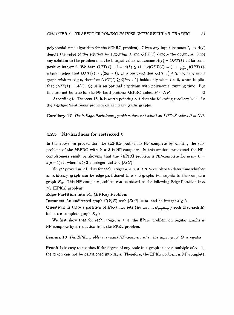
CHAPTER 4. TRAFFIC GROOMING IN UPSR WITH REGULAR TRAFFIC 54
polynomial time algorithm for the kEPRG problem). Given any input instance I, let A(I)
denote the value of the solution by algorithm A and OPT(I) denote the optimum. Since
any solution to the problem must be integral value, we assume A(I) = OPT(I) + i for some
positive integer i. We have OPT(I) + i = A(I) ~ (1 + f)OPT(I) = (1 + 2~+l)OPT(I),
which implies that OPT(I) ~ i(2m + 1). It is observed that OPT(I) ~ 2m for any input
graph with m edges, therefore OPT(I) ~ i(2m + 1) holds only when i = 0, which implies
that OPT(I) = A(I). So A is an optimal algorithm with polynomial running time. But
this can not be true for the NP-hard problem kEPRG unless P = N P. 0
According to Theorem 16, it is worth pointing out that the following corollary holds for
the k-Edge-Partitioning problem on arbitrary traffic graphs.
Corollary 17 The k-Edge-Partitioning problem does not admit an FPTAS unless P = N P.
4.2.3 NP-hardness for restricted k
In the above we proved that the kEPRG problem is NP-complete by showing the sub
problem of the kEPRG with k = 3 is NP-complete. In this section, we extend the NP
completeness result by showing that the kEPRG problem is NP-complete for every k =
a(a - 1)/2, where a ~ 3 is integer and k < IE(G)I.
Holyer proved in [31J that for each integer a ~ 3, it is NP-complete to determine whether
an arbitrary graph can be edge-partitioned into sub-graphs isomorphic to the complete
graph K a . This NP-complete problem can be stated as the following Edge-Partition into
K a (EPKa) problem:
Edge-Partition into K a (EPKa) Problem
Instance: An undirected graph G(V, E) with IE(G)I = m, and an integer a ~ 3.
Question: Is there a partition of E(G) into sets {El,E2, ... ,E_m_} such that each Eia(a-I)/2
induces a complete graph K a ?
We first show that for each integer a ~ 3, the EPKa problem on regular graphs is
NP-complete by a reduction from the EPKa problem.
Lemma 18 The EPKa problem remains NP-complete when the input graph G is regular.
Proof: It is easy to see that if the degree of any node in a graph is not a multiple of a - 1,
the graph can not be partitioned into Ka's. Therefore, the EPKa problem is NP-complete
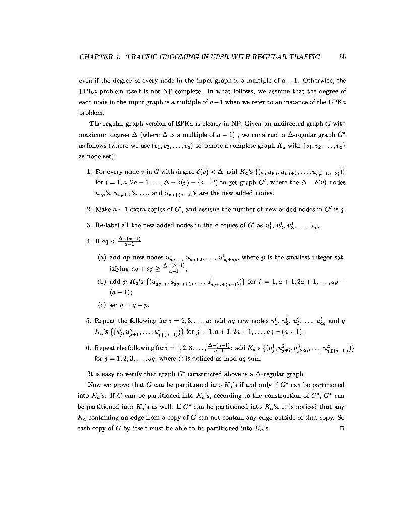
CHAPTER 4. TRAFFIC GROOMING IN UPSR WITH REGULAR TRAFFIC 55
even if the degree of every node in the input graph is a multiple of a - 1. Otherwise, the
EPKa problem itself is not NP-complete. In what follows, we assume that the degree of
each node in the input graph is a multiple of a-I when we refer to an instance of the EPKa
problem.
The regular graph version of EPKa is clearly in NP. Given an undirected graph G with
maximum degree 6 (where 6 is a multiple of a-I) , we construct a 6-regular graph G*
as follows (where we use (VI, V2, ... , Va) to denote a complete graph K a with {VI, V2, ... ,Va}
as node set):
1. For every node V in G with degree <5(v) < 6, add Ka's {(v, Uv,i, Uv,i+I,···, Uv,i+(a-2j)}
for i = 1, a, 2a - 1, ... ,6 - <5(v) - (a - 2) to get graph G', where the 6 - <5(v) nodes
Uv,i'S, Uv,i+I'S, ... , and Uv,i+(a-2j'S are the new added nodes.
2. Make a-I extra copies of G', and assume the number of new added nodes in G' is q.
3. Re-label all the new added nodes in the a copies of G' as uL u~, u§, ... , U~q'
4 If ~-(a-Ij. aq < a I
(a) add ap new nodes U~q+l' U~q+2' ,. " U~q+ap, where p is the smallest integer sat-. f . > ~-(a-l)IS ymg aq + ap _ a-I;
(b) add p Ka's {(U~q+i'U~q+i+l' ... , U~q+i+(a-l))} for i = 1, a + 1, 2a + 1, ... ,ap
(a - 1);
(c) set q = q + p.
5. Repeat the following for i = 2,3, ... , a: add aq new nodes ui, u~, u~, ... , U~q and q
Ka's {(u;, u;+l"'" u~+(a-l))} for j = 1, a + 1, 2a + 1, ... , aq - (a - 1);
6 R h l' 11 . l' • - 1 2 3 ~-(a-l). dd K' {( I 2 3 a )}. epeatt elO owmg lOr z - , " ... , a-I . a as Uj,UjEBi,UjEB2;,,,,,UjEB(a_lji
for j = 1,2,3, ... , aq, where EB is defined as mod aq sum.
It is easy to verify that graph G* constructed above is a 6-regular graph.
Now we prove that G can be partitioned into Ka's if and only if G* can be partitioned
into Ka's. If G can be partitioned into Ka's, according to the construction of G*, G* can
be partitioned into Ka's as well. If G* can be partitioned into Ka's, it is noticed that any
K a containing an edge from a copy of G can not contain any edge outside of that copy. So
each copy of G by itself must be able to be partitioned into Ka's. 0
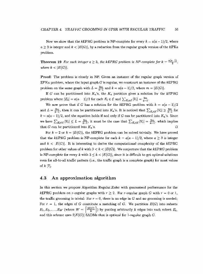
CHAPTER 4. TRAFFIC GROOMING IN UPSR WITH REGULAR TRAFFIC 56
Now we show that the kEPRG problem is NP-complete for every k = a(a -1)/2, where
a ~ 3 is integer and k < IE(G)I, by a reduction from the regular graph version of the EPKa
problem.
Theorem 19 For each integer a ~ 3, the kEPRG problem is NP-complete for k = a(a2-1),
where k < IE(G)I.
Proof: The problem is clearly in NP. Given an instance of the regular graph version of
EPKa problem, where the input graph G is regular, we construct an instance of the kEPRG
problem on the same graph with L = ;~ and k = a(a - 1)/2, where m = IE(G)I.
If G can be partitioned into Ka's, the K a partition gives a solution for the kEPRG
problem where IEil = a(a - 1)/2 for each Ei E £ and L:EiEt: IViI = ;~.
We now prove that if G has a solution for the kEPRG problem with k = a(a - 1)/2
and L = ;~, then it can be partitioned into Ka's. It is noticed that L:EiEt: IViI ~ ;:'1 for
k = a(a-I) /2, and the equation holds if and only if G can be partitioned into Ka's. Since
we have L:EiEt: IViI ::; L = ;~, it must be the case that L:EiEt: IViI = ;~, which implies
that G can be partitioned into Ka's. 0
For k = 2 or k = IE(G)I, the kEPRG problem can be solved trivially. We have proved
that the kEPRG problem is NP-complete for each k = a(a - 1)/2, where a ~ 3 is integer
and k < IE(G) I. It is interesting to derive the computational complexity of the kEPRG
problem for other values of k with 3 < k < IE(G)I. We conjecture that the kEPRG problem
is NP-complete for every k with 3 ::; k < IE(G)I, since it is difficult to get optimal solutions
even for all-to-all traffic pattern (i.e., the traffic graph is a complete graph) for most values
of k [7].
4.3 An approximation algorithm
In this section we propose Algorithm Regular-Euler with guaranteed performance for the
kEPRG problem on r-regular graphs with r ~ 2. For r-regular graph G with r = 0 or 1,
the traffic grooming is trivial: For r = 0, there is no edge in G and no grooming is needed;
For r = 1, the edges of G constitute a matching of G. We partition E(G) into subsets
E1,E2, ... ,Ew (where W = r'E~G)'l) by putting arbitrarily k edges into each subset Ei,
and this scheme uses 2IE(G)1 SADMs that is optimal for I-regular graph G.
CHAPTER 4. TRAFFIC GROOMING IN UPSR WITH REGULAR TRAFFIC 57
For the k-Edge-Partitioning problem on arbitrary traffic graphs, several algorithms have
been proposed in [11, 28]. Intuitively, to achieve good solutions for the k-Edge-Partitioning
problem, we need to partition the traffic graph G into sub-graphs of at most k edges such
that each sub-graph contains as few nodes as possible. One key observation is that given a
fixed number of edges, a sub-graph with fewer components more likely contains fewer nodes.
This is the basic idea behind the algorithms in [11, 28]. Our algorithm Regular_Euler utilizes
a similar idea, and aims to minimize the total number of components over all sub-graphs.
The algorithm uses at most f1E(G)I(l + t)l SADMs for even r ~ 2, and f1E(G)I(1 + Vl +(2(;~1) -1) SADMs for odd r ~ 3, which are almost always better than previous algorithms
applying on regular graphs.
First, we prove the following lemma about the lower bound on the size of the maximum
matching of regular graphs. This lemma also gives a solution for one of the open problems
proposed by Biedl et al. [10].
Lemma 20 A r-regular graph G with IV(G)I = n has a maximum matching containing at
least ~ . r~l edges.
Proof: It is proved by Vizing [49] that any simple graph G has an edge coloring with ~
or ~ + 1 colors, where ~ is the maximum degree of G. The proof immediately yields an
approximation algorithm to color any simple graph G with at most ~ + 1 colors. Therefore,
a r-regular graph G can be colored by r + 1 colors. Considering such an edge coloring, we
notice that each set of edges with the same color is a matching of G. Since the total number
of edges in G is ~, there must exist at least ~1; = ~ . r~l edges having the same color in
the edge coloring. Therefore, ~ . r~l is a lower bound on the size of the maximum matching
of r-regular graph. 0
We prove the following lemma for r-regular graphs.
Lemma 21 For r-regular graph G with IV(G)I = nand r ~ 2, there exists a skeleton cover
of size one if r is even, and there exists a skeleton cover of size at most 2(;~1) if r is odd.
Proof: For even value r (where r -I- 0), we can construct an Euler path of G. Such an Euler
path is a skeleton of G without branches, therefore we obtain a skeleton cover of size one.
For odd value r (where r -I- 1), we first compute a maximum matching M of G. Then
after deleting the edges in M from graph G, all the nodes saturated by M have degree r - 1,
all the unsaturated nodes have degree r, and there might be more than one components in
CHAPTER 4. TRAFFIC GROOMING IN UPSR WITH REGULAR TRAFFIC 58
graph G(V(G), E(G)\M). We call a component in G(V(G), E(G)\M) an even component
if every node in the component has degree r - 1, and an odd component if there exists
a node with degree r. Assume there are s even components and t odd components. Let
Ceven = {C~, C;, ... , C~} be the set of even components, and Codd = {Cl, C2, ... ,Cd be the
set of odd components. It is noticed that there are (n - 21M!) odd-degree (i.e., the degree
is r) nodes in the odd components, and every odd component Ci (1 ::; i ::; t) contains at
least two nodes Vi,l, Vi,2 with degree r since the number of odd-degree nodes in any graph
must be even. We add (n - 2IM!)/2 - 1 virtual edges to change (n - 21M!) - 2 odd-degree
nodes to even-degree nodes (i.e., nodes with degree r+ 1) and connect the t odd components
together into a connected graph Godd at the same time. More specifically, we first add t - 1
virtual edges (Vl,1,v2,I),(V2,2,v3,I), ... ,(Vt-2,2,Vt-l,I),(Vt-l,2,Vt,I) to connect the connect
the odd components into one connected graph. Then for every pair of remaining odd-degree
nodes except Vl,2 and Vt,2, we add a virtual edge between them. It is obvious that the
new generated graph Godd is connected and has exactly two odd-degree nodes vl,2 and Vt,2.
Therefore, an Euler path of Godd can be found. For every even component, we can find
an Euler path as well since each node of the component has even degree r - 1. Taking
the s + 1 Euler paths as the backbones, we can construct a skeleton cover of size s + 1.
After deleting the (n - 2IM!)/2 - 1 virtual edges, we obtain a skeleton cover of G with size
(s + 1) + (n-;IMI - 1) = s + n-;IMI.
Since each node in an even component has degree r - 1, each even component must
contain at least r nodes. In graph G(V(G), E(G)\M), the total number of nodes with
degree r - 1 is 21MI, so the number of even components in graph G(V(G), E(G)\M) is at
most 21~1, that is, s ::; 21~1.
We have IMI ~ ~ . r~l according to Lemma 20, so the size of the skeleton cover for odd
value r is
n - 21MI 21M I n - 21MI (4 - 2r)IMI + nr (4 - 2r) . ~ . r~l + nr 3ns+ < --+ = < = ----,-----,-
2 - r 2· 2r - 2r 2(r + 1)
o
The pseudo code of Algorithm Regular_Euler is given in Figure 4.2.
Theorem 22 Algorithm Regular_Euler finds a k-edge partition E = {El , ... , Ew} of r
regular graph G with W = f'EtG)'l, IEil = k for 1 ::; i < W, L:E;Et: l\til ::; fI E (G)I(1 + Vlfor even r ~ 2, and L:E;Et: I\til ::; f1E(G)I(1 + t)l + (2d~1) - 1) for odd r ~ 3.
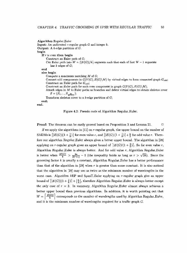
CHAPTER 4. TRAFFIC GROOMING IN UPSR WITH REGULAR TRAFFIC 59
Algorithm Regular...EulerInput: An undirected r-regular graph G and integer k.Output: A k-edge partition of G.begin
If r is even then beginConstruct an Euler path of G;Cut Euler path into W = r1E(G)I/kl segments such that each of first W - 1 segments
has k edges of G;endelse begin
Compute a maximum matching M of G;Connect odd components in G(V(G), E(G)\M) by virtual edges to form connected graph Godd;Construct an Euler path for Godd;Construct an Euler path for each even component in graph G(V(G), E(G)\M);Attach edges in M to Euler paths as branches and delete virtual edges to obtain skeleton cover
S = {Sl, ... , S 3n };2(r+l)
Transform skeleton cover to a k-edge partition of G;end;
end.
Figure 4.2: Pseudo code of Algorithm Regular_Euler.
Proof: The theorem can be easily proved based on Proposition 3 and Lemma 21. 0
If we apply the algorithms in [11] on r-regular graph, the upper bound on the number of
SADMs is f1E(G)I(1 + til for even value r, and rIE(G)I(1 + *)1 +~ for odd value r. There
fore our algorithm Regular_Euler always gives a better upper bound. The algorithm in [28]
applying on r-regular graph gives an upper bound of rIE(G)I(1 + f)l So for even value r,
Algorithm Regular_Euler is always better. And for odd value r, Algorithm Regular-Euler
is better when IE1G)1 > 2d~1) - 1 (the inequality holds as long as r > J3k"). Since the
grooming factor k is usually a constant, Algorithm Regular_Euler has a better performance
than that of the algorithm in [28] when r is greater than some constant. It is also noticed
that the algorithm in [28] may use as twice as the minimum number of wavelengths in the
worst case. Algorithm kEP and SpanT..Euler applying on r-regular graph give an upper
bound of fI E(G) I(1 + *)1 + l~J' therefore Algorithm Regular..Euler is always better except
the only case of r = 3. In summary, Algorithm Regular..Euler almost always achieves a
better upper bound than previous algorithms. In addition, it is worth pointing out that
W = r,E1G)ll corresponds to the number of wavelengths used by Algorithm Regular-Euler,
and it is the minimum number of wavelengths required for a traffic graph G.
CHAPTER 4. TRAFFIC GROOMING IN UPSR WITH REGULAR TRAFFIC 60
A maximum matching can be computed in O([vI~IE(G)1) time, the Euler path con
struction can be done in O(IE(G)I), and each of other steps in Algorithm Regular-Euler
can be done in O(IE(G)I) as well, therefore Algorithm Regular-Euler runs in O([vI~ IE(G)I)
time.
4.4 Empirical results
In this section, we will conduct extensive simulations to evaluate the practical performance
of our algorithm by comparing to existing algorithms. We implemented the algorithms
in [11, 28], Algorithm kEP, Algorithm SpanT-Euler and Algorithm Regular-Euler to com
pare their performances on regular traffic graphs randomly generated by the regular graph
generator from [2]. Figure 4.3 shows the empirical results for graphs of 36 nodes with dif
ferent settings of degree r and grooming factor k, where for each value of rand k we collect
the results from 100 randomly generated regular graphs and compute the average value.
For Algorithm Regular-Euler, the confidence level for confidence interval [1-5%,1+5%] is
about 94%. We refer to the algorithm in [28] and [11] as Algo. 1 and Algo. 2 respectively.
The empirical results in Figure 4.3 verify that Algorithm Regular-Euler outperforms most
of other algorithms (it is also observed that the performance of Algo. 2 is close to that
of Algorithm Regular-Euler in most cases, which is due to the fact that both algorithms
are Euler-path based algorithms. However, as we showed in the previous section, the worst
case performance of Algorithm Regular-Euler is always better than that of Algo. 2). We
ran simulations on graphs with different parameter settings as well, and the results present
similar characteristics (see Figure 4.4 and Figure 4.5 for some representative results).
In Section 4.3 we showed that Algorithm Regular_Euler achieves a provable upper bound
for the kEPRG problem, where the upper bound measures the worst case performance of
the algorithm. We compare this worst case upper bound to the average performance of
Algorithm Regular-Euler in Figure 4.6. We also include a lower bound for the kEPRG
problem in the Figure. The lower bound is derived based on a lower bound for the k-Edge
Partitioning problem given in [28]. Goldschmidt et ai. [28] established the lower bound for
k-Edge-Partitioning problem by observing that each sub-graph in the best possible k-edge
partition is a complete graph with exactly k edges. Therefore, the total number of nodes
over all sub-graphs is bounded below by IE~G)I . l+~. Given an integer a such that
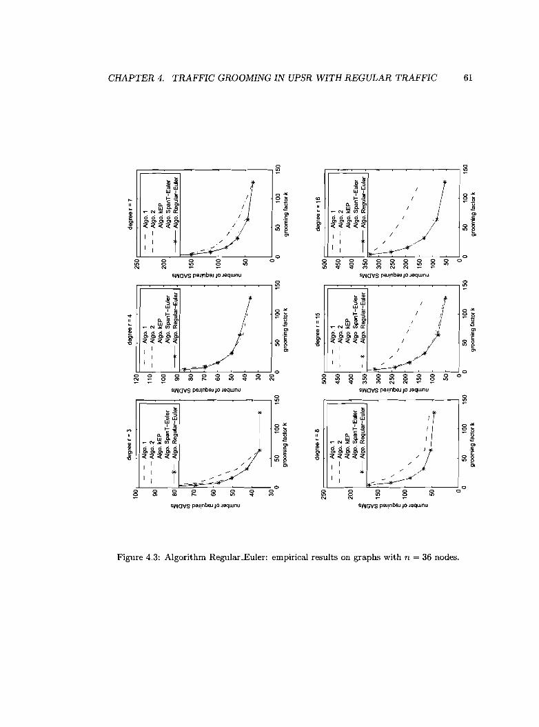
"rj
@oq
'~
degr
eer
=3
degr
eer=
4de
gree
r=
7'i::
l~
10
01
20
25
0
~"1 (1
)-
-A
lga.
1-
-A
lga.
1-
-A
lga.
1~
--
-A
lga.
21
10
-A
lga.
2-
Alg
a.2
~
""9
0A
lga.
kEP
Alg
a.kE
PA
lga.
kEP
....1
00
20
0;J>
Alg
a.S
panT
-Eu
ler
Alg
a.S
panT
-Eu
ler
Alg
a.S
panT
-Eu
ler
oq..
80
----
+--
Alg
a.R
eg
ula
r-E
ule
r'"
----
-lif
-A
lga.
Re
gu
lar-
Eu
ler
..--
---l
if-
Alg
a.R
eg
ula
r-E
ule
r
~::;
::;9
0::;
00
00
"1«
I«
«:;+
:en
70
\en
80
~1
50
'0'0
I"r
j::r
-e!
e!e!
S'5
1\'5
70
'5\
~0
'0
'0
'
::0e!
60
\e!
e!\
CJ(1
)0
\'0
60
'01
00
,G
Q'q
:;;:;;
:;;~
~.0
\.0
50
.0"-
~E
50
EE
"-0
"\
""
cc
c~
0I
,4
0-
-5
0tr:I
40
,~
~ m--
----
--4
30
~:: (1
)3
020
0
~S
05
01
00
15
00
50
10
015
00
50
10
01
50
'E.
groo
min
gfa
ctor
kgr
oom
ing
fact
ork
groo
min
gfa
ctor
k
~::1
.()
~~ "1
degr
eer
=8
degr
eer=1
5de
gree
r=1
6
~(1
)00
25
05
00
50
0~ :;:;
:'-
-A
lga.
1-
-A
lga.
1-
-A
lga.
1~
00-
Alg
a.2
45
0-
--
Alg
a.2
45
0'-
Alg
a.2
0A
lga.
kEP
Alg
a.kE
PA
lga.
kEP
~l:I
20
04
00
40
0Q
'qA
lga.
Spa
nT-E
ule
rA
lga.
Spa
nT-E
ule
rA
lga.
Spa
nT-E
ule
rt.'l:
'J"1
..--
Alg
a.R
eg
ula
r-E
ule
r'"
----
-lif
-A
lga.
Re
gu
lar-
Eu
ler
'"--
---l
if-
Alg
a,R
eg
ula
r-E
ule
rG
\l>::;
::;3
50
::;"d
Cl
00
~::r-
««
«en
~3
00
en00
'0\
'0~
~e!
e!e!
,~
'5.~
25
0,
.~
25
0"-
:;+:
0'
"-;5
::r-e!
e!'-
e!'0
'02
00
~
'0'-
;:l
'-~
1i;,
:;;'-
:;;~
~II
.0,
~1
50
,~
~1
50
'-"r
jE
'-
"""
~
-"
"~
cc
cC
t.l50
10
0""
10
0CJ
l:I- -
05
0-
50
Q..
(1)
~0
00
05
01
00
15
00
501
00
15
00
50
10
01
50
Ct.l
groo
min
gfa
ctor
kgr
oom
ing
fact
ork
groo
min
gfa
ctor
kI-'
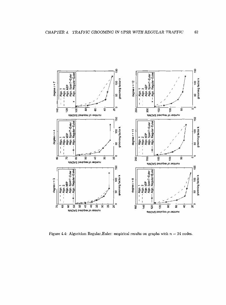
"!j
g ~ciG
°d
eg
ree
r=3
degr
eer=4
de
gre
er=7
'i:l
~70
8014
0~
.... ell
--
Alg
a.1
--
Alg
a.1
Alg
a.1
.+:.
65-
--
Alg
a.2
--
-Alg
a.
2-
--
Alg
a.2
::0~
Alg
a.kE
P70
Alg
a.kE
P12
0A
lga.
kEP
11>0.
III
60II
III
I
>::2
Alg
a.S
pa
nT
-Eu
ler
::2A
lga.
Sp
an
T-E
ule
r::2
Alg
a.S
panT
-Eu
ler
ciG~
55--
--+
-Alg
a.R
eg
ula
r-E
ule
Cl
----
+-A
lga.
Re
gu
lar-
Eu
leC
l--
--+
-A
lga.
Re
gu
lar-
Eu
le~
0;:j
60;:j
100
....~
50\
'C'C
~~
~\
~\
..",
::r'
.~4
5~
'S'S
~S
~50
\0
'80
\~
\~
0::t
I~
40'0
'0el
l\
.840
Q;Q
(Tq
II>\
E.-.0
.\.0
::0E
35E
E....
0'"
:;,
~\
:;,
\:;
,....
....c:
"-c:
c:0
f:.j30
"-30
e;40
~
""-
CD25
"-<
~Q
ell
2020
20
~S
050
100
150
050
100
150
050
100
150
"dgr
oom
ing
fact
ork
gro
om
ing
fact
or
kgr
oom
ing
fact
or
k
sa::;
0 n° e:-ga
....de
gree
r=8
degr
eer=1
1de
gree
r=1
2:§
ell
r:n16
025
025
0~ :;:
;:'-
-A
lga.
1-
-A
lga.
1-
-A
lga.
1~
r:n-
--A
lga
.2
--
-Alg
a.
2-
--
Alg
a.2
014
0A
lga.
kEP
Alg
a.kE
PA
lga.
kEP
::0;:
lII
I20
0II
I20
0II
IA
lga.
Spa
nT-E
ule
rA
lga.
Sp
an
T-E
ule
rA
lga.
Sp
an
T-E
ule
rtr:
l(T
q::2
::2::2
....S!
120
----
+-A
lga.
Re
gu
lar-
Eu
leC
l--+
-A
lga.
Re
gu
lar-
Eu
leC
l_
-A
lga.
Re
gu
lar-
Eu
leQ
'"<t
;:j8
"drJ
)rJ
)
~~'"
::r'
'C'C
~15
0r:n
.~10
0\
~~
~.:;
,\
'S'S
::00
'0
'0
'rt
~e
~
~::r
''0
'0"-
'010
0;:3
Q;Q;
"-.8
II.0
.0"-
..",
E\
E"-
EtV
:;,
\:;
,"-
:;,
~.+
:.c:
c:c:
\50
"-50
0;:
l40
"-~
0 0-
"-
ell ?'
20'
0'
I0
050
100
150
050
100
150
050
100
150
0":>
groo
min
gfa
ctor
kgr
oom
ing
fact
or
kg
room
ing
fact
or
ktV
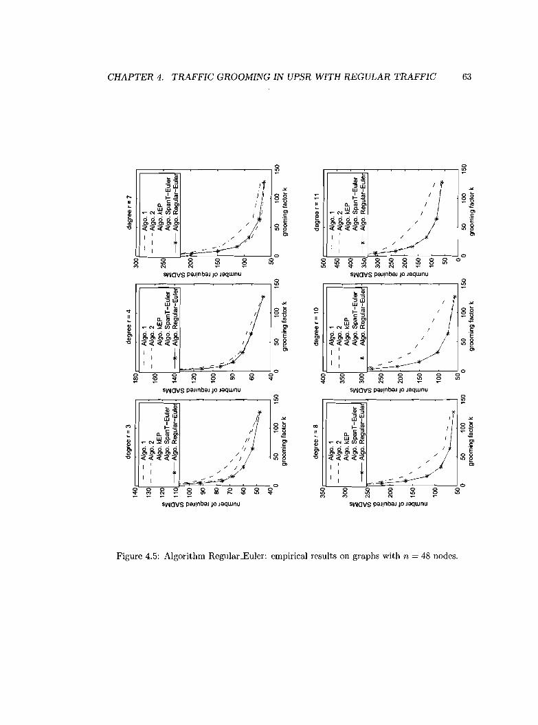
'Tj
~ >aq
"d
eg
ree
r=3
de
gre
er=4
de
gre
er=7
'i:lI::
140
180
300
~...., ro
--
Alg
o.1
--
Alg
o.1
--
A1g
o.1
..,.13
0-
--
Alg
o.2
--
-Alg
o.
2-
--A
1g
o.2
::0C
JlA
lgo.
kEP
160
Alg
o.kE
PA
1go.
kEP
~en
120
enen
250
>::E
Alg
o.S
pa
nT
-Eu
ler
::EA
lgo.
Sp
an
T-E
ule
r::E
A1g
o.S
pa
nT
-Eu
ler
aq~
110
----
-lI<
--A
lgo.
Re
gu
lar-
Eu
le~
140
----
-lI<
--A
lgo.
Re
gu
lar-
Eu
lec
----
-lI<
--A
1go.
Re
gu
lar-
Eu
le~
<I:
0(/
)(/
)(/
)....,
ijl10
0"C
¥20
0>
~.~
120
'"11::
r'.=
\a
:l
:l
'S~
0"
90.\
0"
0"
\
~~
\\
~\
~Q
'0'0
100
~15
0\
Q;80
\G
aq\
Q;<I>
\::0
I::.0
.0.0
~E
70"-
EE
\0
:l
"-"-
:l
:l
....,c:
-c:
c:"-
0I
60.;
:--
100
tr:I-
"-E5
---
I::--
--
--
ro-50
:::,..
.~
--.
-~
....,-
-ro
40
40
50
S2a
050
100
150
050
100
150
050
100
150
'C:I
groo
min
gfa
ctor
kgr
oom
ing
fact
or
kgr
oom
ing
fact
ork
~::;" n' 2:-
~....,
de
gre
er=8
de
gre
er=1
0d
eg
ree
r=1
1:§
<0 CJl
350
400
500
e- M-
--
Alg
o.1
--
Alg
o.1
--
A1g
o.1
~CJ
l-
Alg
o.2
--
-Alg
o.2
450
--
-A1
go
.2
035
0::l
300
Alg
o.kE
PA
lgo
.kE
Pen
400
Alg
o.kE
P::0
enA
lgo.
Sp
an
T-E
ule
ren
Alg
o.S
pa
nT
-Eu
ler
Alg
o.S
panT
-EuJ
ertr
laq
::E::E
::E....,
C--
-+-
Alg
o.R
eg
ula
r-E
ule
~30
0--
-+--
Alg
o.R
eg
ula
r-E
ule
r~
350
---+
-A
1go.
Re
gu
lar-
Eu
leG
~;Jj
250
~'C
:I(/
)(/
)::
r'"C
"C¥
300
CJl
~~
250
\>
§.'S
'S'S
\::0
~20
0\
0"
\~
250
M-
~
~::
r''0
\'0
200
\'0
"-;3
.815
0\
Q;\
Q;"-
>II
.0"-
.0"-
~E
\§
150
E-
..,.:l
"-:l
c:c:
c:-
....(y
j\
-10
0-
Q10
0-
-::l
\10
0-
0~
-50
Po
--
~<0
-?'
5050
00
5010
015
00
5010
015
00
5010
015
0~
groo
min
gfa
ctor
kg
roo
min
gfa
cto
rk
groo
min
gfa
ctor
kc..:
>
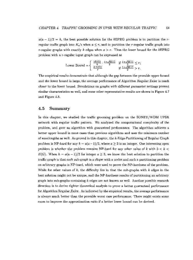
CHAPTER 4. TRAFFIC GROOMING IN UPSR WITH REGULAR TRAFFIC 64
a(a - 1}/2 = k, the best possible solution for the kEPRG problem is to partition the r
regular traffic graph into Ka's when a ~ r, and to partition the r-regular traffic graph into
r-regular graphs with exactly k edges when a > r. Thus the lower bound for the kEPRG
problem with a r-regular input graph can be expressed as
{
IE(G)I. 1+y!8k±I if 1+y!8k±I < r.L B d k 2 2-'
ower oun = 2IE (G)[ • 1 vtsk+l8k1r If + 2 + > r.
The empirical results demonstrate that although the gap between the provable upper bound
and the lower bound is large, the average performance of Algorithm Regular-Euler is much
closer to the lower bound. Simulations on graphs with different parameter settings present
similar characteristics as well, and some other representative results are shown in Figure 4.7
and Figure 4.8.
4.5 Summary
In this chapter, we studied the traffic grooming problem on the SONET/WDM UPSR
network with regular traffic pattern. We analyzed the computational complexity of the
problem, and gave an algorithm with guaranteed performance. The algorithm achieves a
better upper bound in most cases than previous algorithms and uses the minimum number
of wavelengths as well. As proved in this chapter, the k-Edge-Partitioning of Regular Graph
problem is NP-hard for any k = a(a -1}/2, where a 2: 3 is an integer. One interesting open
problem is whether the problem remains NP-hard for any other value of k with 3 < k <E(G}. When k = a(a - 1}/2 for integer a 2: 3, we know the best solution to partition the
traffic graph is that each sub-graph is a clique with a nodes and such a partitioning problem
on arbitrary graphs is NP-hard, which were used to prove the NP-hardness of the problem.
While for other values of k, the difficulty lies in that the sub-graphs with k edges in the
best solution might not be unique, and the NP-hardness results of partitioning an arbitrary
graph into sub-graphs containing k edges are not known as well. Another possible research
direction is to derive tighter theoretical analysis to prove a better guaranteed performance
for Algorithm Regular-Euler. As indicated by the empirical results, the average performance
is always much better than the provable worst case performance. There might exists some
room to improve the approximation ratio if a better lower bound can be derived.
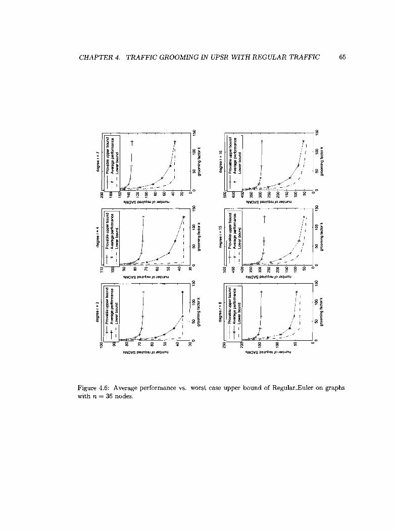
~"I
j
~~
aq'
::r~ ...,
;:l('1)
de
gre
er
=3
degr
eer
=4
degr
eer
=7
'i:l
II~
100
110
200
~c...;~
-+--
Pro
vabl
eup
per
boun
d1
-+--
Pro
vabl
eup
perb
ound
-+--
Pro
vabl
eup
per
boun
d1
0)
9~
----
---=
.f--
Ave
rage
perf
orm
ance
1---
----=
.f--
Ave
rage
perf
orm
ance
18~
----
---'
;f--
Ave
rage
perf
orm
ance
::0:::J
;..--
-L~er
boun
d.
-.
-Lo
wer
boun
d-
-Lo
wer
boun
d~
0<
1
~0
.('1
)i
80i
~14
0
~CD
...,
UJ~
00
.()q
~70~
««
I~CD
rnrn
120
~~
~'0
·5·5
g.1
00
1\
~CD
"I
"~
...,I!!
I!!I!!
I~
8''5
60*
'5'5
80G
...,.8
.8.8
i\
SE
00[\
E§
60\~
G~
""
::0:::J
c;c;
50c;
"_._~
0n
40CD
40.
10
<\
.4
020
~~
._.-
-*I:
\_
._._
.--
-
~3
030
0~
050
100
150
050
100
150
050
100
150
G...,
groo
min
gfa
ctor
kgr
oom
ing
fad
ark
groo
min
gfa
ctor
k
~U
J .... n
~~ U
J CDde
gree
r=
8de
gree
r=15
de
gre
er
=16
~~
250
500
5llO
'0-+
--P
rova
ble
uppe
rbo
undI
4~
-+--
Pro
vabl
eup
perb
ound
I.4s
o1-+
--
Pro
vabl
eu
pp
erb
ound
I.~
'0---
---+-
--A
vera
gepe
rfor
man
ce--
----
-'¥--
--A
vera
gepe
rfor
man
ce--
----
-'if-
-A
vera
gepe
rfor
man
ceCD ...,
-.
-Lo
wer
boun
d.-
.-
Low
erbo
und
--
Low
erbo
und
204
4
~0
"i
~35
0~
350
0
kl
k~
0::0
:::J~
««
rnrn
tr.10
."
150
\~
300
~30
0I!!
KG
0·5
~.~
250
I,~
250
.....~
I!!it\
I!!~
~'0
100
1\
'520
0'5
200
>CD
1i1
\.8
\\
.81\
()q
\\
::0~
§I\
--.
§15
0§
150
\\.
Sl
c;c;
\\"
c;.
~...,
50"-~~
100
100
"-"..
~-------
~--
-.,.
"-.~~,.
\.._
.-
--
-~
5050
-.-.
-.-
-=-~
,.
~ro
--
-'...,
00
0....
00
5010
015
00
5010
015
00
5010
015
0G
:::Jgr
oom
ing
fact
ork
groo
min
gfa
ctor
kgr
oom
ing
fact
ork
()q ..., ~ '0 ::r
0)
UJ
Cl1
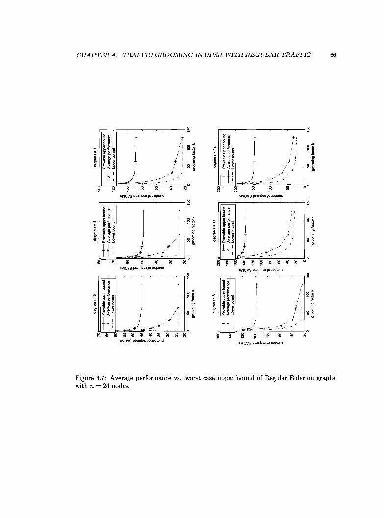
Ol
Ol@ > '"tl ~ ::0 ~ ~ > ~ G ga o o ~ 8 ~ ~ ~ ~ ~ ~ G 8 > ::0 ~ > ~
150
150
de
gre
er=
12
5010
0gr
oom
ing
fact
ork
5010
0gr
oom
ing
fact
ork
\.~
"~~--t
\
0'
I
o
20o
25
0,=
==
==
==
:;-]
---+
---
Pro
vabl
eup
per
boun
d---
----+
--A
vera
gepe
rfor
man
ce-
.-L
ow
er
boun
d
loo~ \\
--+
-1
-~I-
80~ 1\
60
fl
\ \\~
40
f\,_._<~
degr
eer=
7
14
0,=
==
==
==
=:;-]
---+
---Prova~e
uppe
rbo
und
------
-+--
Ave
rage
perf
orm
ance
12~
_.
-L
ow
er
boun
dIi
~~
'g15
0i\ "t II.
, i\ 11,
'5 C'
f ~10
01l E ~ "
50
150
~o
100
groo
min
gfa
cto
rk
40 2020L
'__~
~_
_-.
J
o
de
gre
er
=4
80--
-+--
-P
rova
ble
uppe
rbo
und
------
-"¥-
---A
vera
gepe
rfor
man
ce7
-,-
Lo
we
rbo
und
~ 0 « en ~ '5 C' e '0
.840
1\.8
E.
E~
1,,-
~ "30
I'"
,,-
I._.~-
O'L
-__~
__~~
__
...J
o50
100
150
groo
min
gfa
ctor
k
de
gre
er
=11
2o
o',
Jl=
==
==
==
::::
:;l
---+
---
Pro
vabl
eup
per
boun
d---
----+
--A
vera
gepe
rfor
man
ce
16-
Lo
we
rbo
und
i
~14
0'i
«I'
'g12
0~
~,
.~10
0i\
e''
.~
80\'\
1l'
E60
\'\
~\
""
'-~
......._
_.::
-:-::1
degr
eer=
8
401601,=======~
--+
--P
rova
ble
up
pe
rbou
nd
14~
t=g~,:nnance
~55 i:~
!\
~40
11l
.~
§3
5'
""
I\
30i
\~',
-25
I._
._::-
.,.,,
_
20L
-__~
__
~_-----.J
o50
100
150
groo
min
gfa
ctor
k
de
gre
er=
37
0',
==
==
==
=:;"""]
--+
--P
rova
ble
uppe
rbo
und
6---
----+
--A
V8r
nge
perf
onna
nce
-,
-L~bound
l12
0I
« enI
-g10
0'>1
.~~\
e..
-80
"~
\\
".,
.Qi,
EI'
~60
\'\ \\
l<'__'
,~
20
'~._._._~
o50
100
150
groo
min
gfa
ctor
k
~ .., r:JJ
rt
(")
~ r:JJ
CD >::: "0 "0 CD .., cr'
o >::: ::l 0..
o -, ; >::: ~ ~ >::: ro .., o ::l ~ .§ :::r'
r:JJ
:;:~
;;:
&q"
:::r'>
:::~
@II~
~:;l
::l>
o<
0..
CDCD
..,
r:JJ
Jcl CD "0 ~ 0' .., S § ~ ~
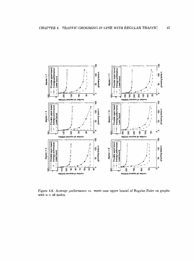
de
gre
er=3
de
gre
er=4
de
gre
er=7
140
160
300
--+
--P
rova
ble
up
pe
rbo
und
--+
--P
rova
ble
up
pe
rbo
und
--+
--P
rova
ble
up
pe
rbo
undI
1_
_A
vera
ge
pe
rfo
rma
nce
--
Ave
rag
ep
erf
orm
an
ce--
Ave
rag
ep
erf
orm
an
ce-
.-L
ow
er
boun
d1
--
Lo
we
rb
ou
nd
.-
.-
Lo
we
rbo
und
1In
InIn
::;::;
::;~
110
0
~,oo
ten
;:J12
0"0
"0"0
I~
~
-i150
1+'S
'5"!
CY
~10
0\
i!!!
'\"0
"0.
o\
'Iii
.880
I.8
100
i"\,
.0 E
i:~~~
~JI,~-=~
::> <::
60I
._
._
._
._
.-
-'!
'
a.>
--J~ ~ o ::0 o o e; ~ ~ ~ gj ~ ~ ::0 trl o ~ ~ ::0 ;5 ~ '"
rj ~ G@ ;t.:~ ~ ::0 ~
--."
5010
0g
roo
min
gfa
cto
rk
OIL---~--~--...J
o
50
olL--_~_~_--J
o50
100
150
gro
om
ing
fact
or
k
~--+
--P
rova
ble
up
pe
rbO
U 1d--
Ave
rag
ep
erf
orm
an
ce-
.-L
ow
er
boun
d
de
gre
er=
1150
0
In ::; o35
0;:J "0
300
i!!I
_+.~
2501
-520
0i\
il\~
E15
01
\
E*'
100
\~
",,*---
'-.~--------._~
de
gre
er=
10
50,
--+
--P
rova
ble
up
pe
rbo
undI
--
Ave
rag
ep
erf
orm
an
ce.-
.-
Lo
we
rb
ou
nd
OLI
~_
_~-_---.J
o50
100
150
gro
om
ing
fact
or
k
40'
I
o50
100
150
gro
om
ing
fact
or
k
400
~30
0o «
I
~25
0i
Ql
Ii
.~20
0ttl
Ql
.
.::II
~15
0i\,
.0.~
E1
E10
0,
150
5010
0g
roo
min
gfa
cto
rk
40L
I__~
~_-----.J
o
de
gre
er=
8
--+
--P
rova
ble
up
pe
rbo
undI
--
Ave
rag
ep
erf
orm
an
ce-
-L
ow
er
boun
d
OL
I~
__~---
o50
100
150
gro
om
ing
fact
or
k
50300
In ::; ~2
00
1""----t------j-
enII
"0'1
.~~
5-15
01\
jl00\\~
§1
I::
,,_
~
::0 (1)
oq ~ ~ ..., M ~ ro ..., o ::s oq ..., .§ g'
~ U1 <+ n g; (1)
~ :g (1) ..., cr'
o ~ ::s p.. o ......
:;:"'
:j::;
:ciG
P"'~
;3til
II...
~9?
::s>
o<:
p..
(1
)(1
)...
,en
P>-o
q (1)
"0 ~ 0'
..., S § g a
Chapter 5
Min-Max and Max Throughput
traffic grooming
In the previous two chapters, we have studied the traffic grooming problem to minimize
the total number of used SADMs in order to satisfy the full connectivity for a given set
of traffic demands. In this chapter, using novel graph partitioning approaches, we study
traffic grooming from different point of views. We first consider a Min-Max optimization
problem to minimize the maximum number of required SADMs at a network node over all
network nodes. We focus on the Unidirectional Path-Switched Ring (UPSR) network with
unitary duplex traffic demands. We prove the NP-hardness of this minimization problem,
and propose a linear time (kt1 + 2)-approximation algorithm. In addition, we study the
problem to maximize the number of accommodated traffic demands in networks with limited
number of SADMs at each network node. We prove that this maximization problem is NP
hard as well, and propose a (k + I)-approximation algorithm. We also study the all-to-all
traffic pattern, which is an important special case. For both the minimization and the
maximization problems, we give algorithms achieving solutions only constant factors away
from the optimal ones.
68
CHAPTER 5. MIN-MAX AND MAX THROUGHPUT TRAFFIC GROOMING 69
5.1 Problem formulation
We first consider the problem to minimize the maximum number of required SADMs over
all network nodes. A similar Min-Max optimization goal has been discussed for the multi
hop traffic grooming problem [12]. Such a Min-Max traffic grooming problem is of high
practical interest [12]. First of all, minimizing the maximum number of SADMs very likely
produces a homogeneous network design in terms of the number of SADMs at each network
node. Homogeneous nodes usually have lower cost than heterogeneous ones for network
deployment, maintenance and upgrade due to the identical specifications. Furthermore,
the Min-Max optimization goal is important for dealing with dynamic traffic demands. In
particular, if the traffic pattern is changing dynamically within a given set, we can pre
compute a solution for each traffic pattern in the set, and deploy in every node with the
largest number of SADMs required by any solution. Thus any traffic pattern from the given
set can be satisfied without reconfiguring the deployment of SADMs.
We also study the dual problem of the above Min-Max optimization problem: maximize
the throughput for a given set of traffic demands on a network with a limited number of
SADMs at each network node. This problem is critical in the situation that there are no suf
ficient SADMs in the network to satisfy the full connectivity of the traffic demands. Similar
sparse grooming networks are studied in [35, 62, 63, 69], where limited number of grooming
resources are deployed unevenly among network nodes in the network. In this chapter, we
consider homogeneous networks with limited number of grooming resources. Specifically,
we consider the network in which every network node is equipped with a limited number L
of SADMs, and we study the problem to maximize the number of satisfied traffic demands.
Such a Maximum Throughput traffic grooming problem is natural in the WDM network
operation: when the deployed SADMs are not sufficient to satisfy the full connectivity for
a given set of traffic demands, a grooming scheme which satisfies as many traffic demands
as possible is greatly desired.
Recall that for the unitary duplex traffic grooming problem in the UPSR network, a
k-Edge-Partitioning problem has been formulated to minimize the total number of used
SADMs, such that the full connectivity for a given set of traffic demands can be satisfied.
We use a similar graph partition approach for the Min-Max traffic grooming problem. The
Min-Max traffic grooming problem can be formulated as the following Min-Max k-Edge
Partitioning problem (MMkEP) on the traffic graph:

CHAPTER 5. MIN-MAX AND MAX THROUGHPUT TRAFFIC GROOMING 70
Min-Max k-Edge-Partitioning Problem (MMkEP)
Instance: A traffic graph G(V, E) and integer k ~ IE(G)I.
Objective: Partition the edge set E(G) into a collection of pairwise disjoint subsets E =
{El,Ez, . ..} such that IE;I ~ k for each E; E E. The objective is to minimize the value of
max"EV(G) A(v), where A(v) is the number of E;'s each of which contains at least one edge
incident to node v.
It is noticed that integer k corresponds to the grooming factor, each subset E; cor
responds to a wavelength, and A(v) corresponds to the number of used SADMs in node
v.
Similarly, the Maximum Throughput traffic grooming problem can be formulated as the
following Maximum Connectivity k-Edge-Partitioning problem (MaxCkEP) on the traffic
graph:
Maximum Connectivity k-Edge-Partitioning Problem (MaxCkEP)
Instance: A traffic graph G(V, E), an integer k ~ IE(G)I and an integer L.
Objective: Find a collection E = {El' Ez, ...} of pairwise disjoint subsets of E(G) such
that IE;I ~ k for each E; E E and A(v) ~ L for each v E V(G), where A(v) is the number
of E;'s each of which contains at least one edge incident to node v. The objective is to
maximize L:EiE£ IE;I.
It is noticed that integer L corresponds to the number of available SADMs at each node,
and the other parameters have the same meaning as we described in the MMkEP problem.
5.2 Min-Max k-Edge-Partitioning Problem
In this section, we prove that the MMkEP problem is NP-hard, and propose a linear time
(k!l + 2)-approximation algorithm, where k is the grooming factor. In addition, we show
that the algorithm achieves the worst case lower bound for the MMkEP problem. As an
important special case, the all-to-all traffic pattern attracts a lot of research attention as
well. The all-to-all traffic pattern has been well studied for minimizing the total number
of used SADMs [5, 6, 7, 8, 32, 42, 64]. For the all-to-all traffic pattern, the traffic graph
is a complete graph. We prove a lower bound ~ for the MMkEP problem on complete
graph K n , and propose an algorithm achieving an upper bound \II n + ~, which is a~v'2k-z
CHAPTER 5. MIN-MAX AND MAX THROUGHPUT TRAFFIC GROOMING 71
constant factor away from the lower bound. The lower bound is interpreted in the Min-Max
traffic grooming problem as that for the all-to-all traffic pattern on a network of n nodes,
at least ~ SADMs are needed at a network node with the maximum number of SADMs
for any solution. The upper bound says that our algorithm gives a solution which requires
at most If n + ~ SADMs at any node. We also show that the upper bound can be~Y2k-2
systematically improved further for relatively large values of k.
5.2.1 NP-hardness
In this section we analyze the computational complexity of the MMkEP problem. We first
prove that the problem is NP-hard, and then show that the problem does not admit an
FPTAS unless P = N P. We consider the decision version of the MMkEP problem, and
prove that it is NP-complete. The decision version of the MMkEP problem is stated as
follows:
Min-Max k-Edge-Partitioning (MMkEP) Problem
Instance: An undirected graph G(V, E), and integers k, L.
Question: Is there a partition of E(G) into a collection of pairwise disjoint subsets E ={El,E2 ,,,.} such that
1. IEil ~ k for each E i E E, and
2. maxvEV(G) A(v) ~ L, where A(v) is the number of Ei'S each of which contains at least
one edge incident to node v.
We prove that the MMkEP problem is NP-complete by a reduction from the regu
lar graph version of the Edge-Partition into Thiangles (EPT) problem. The regular graph
version of the EPT problem is proved to be NP-complete in Chapter 4 and stated as follows:
Edge-Partition into Triangles (EPT) Problem (regular graph version)
Instance: An undirected r-regular graph G(V, E) with IE(G)I = m.
Question: Is there a partition of E(G) into sets {El, E2, ... , E m / 3 } such that each Ei induces
a triangle?
CHAPTER 5. MIN-MAX AND MAX THROUGHPUT TRAFFIC GROOMING 72
Theorem 23 The MMkEP problem is NP-complete.
Proof: The MMkEP problem is clearly in NP. Given an instance of the regular graph
version of the EPT problem with an undirected input r-regular graph G, we construct an
instance of the MMkEP problem with G as the input graph, k = 3, and L = ~. We prove
that G can be partitioned into triangles if and only if there exists a solution for the MMkEP
problem on the constructed instance.
If G can be partitioned into triangles, it is easy to verify that the triangle partition of
G gives a solution for the MMkEP problem on the constructed instance.
We now prove that if the constructed instance has a solution E = {El' E2, ... } for the
MMkEP problem, then G can be partitioned into triangles. For solution E we have
1. lEd:::; 3 = k for each Ei E E, and
2. maJevEV(G) A(v) :::; ~ = L.
Let Gi denote the sub-graph (of G) induced by each edge set E i E E. We notice that
fV(Gi)1 ~ IE(Gi)1 since each graph Gi contains at most 3 edges, where the equation holds
if and only if Gi is a triangle (Le., the complete graph with three edges). Hence we have
L fV(Gi ) I ~ L IEil = IE(G)I·EiEE EiEE
Therefore
L A(v) = L fV(Gi)1 ~ [E(G)I = rfV~G)I.VEV(G) EiEE
We also know that maJevEV(G) A(v) :::; ~, which implies that
L A(v):::; r ·I~(G)I.vEV(G)
Therefore it must be the case that
L A(v) = r 'I~(G)I,vEV(G)
which implies that every E i E E induces a triangle. That is, graph G can be partitioned
into triangles. 0
We further prove that the MMkEP problem does not admit an FPTAS unless P = N P.
CHAPTER 5. MIN-MAX AND MAX THROUGHPUT TRAFFIC GROOMING 73
Theorem 24 The MMkEP problem does not admit an FPTAS unless P = N P.
Proof: Assume that the MMkEP problem does admit an FPTAS. Now we construct an
algorithm A that calls the FPTAS with precision € = r~l' where r is the maximum degree
of graph G. Since the time complexity of an FPTAS is polynomial in the input size and
also polynomial in ~ = r + 1 and r + 1 is at most O(n), algorithm A is polynomial in the
input size (i.e., an polynomial time algorithm for MMkEP). Given any input instance I, let
A(I) denote the value of the solution by algorithm A and OPT(I) denote the optimum.
Since any solution to the problem must be an integer, we assume A(I) = OPT(I) + i for
some positive integer i. We have OPT(I) +i = A(I) ~ (1 + €)OPT(I) = (1 + r~l )OPT(I) ,
which implies that OPT(I) ~ i(r + 1). It is observed that OPT(I) ~ r for any instance,
therefore OPT(I) ~ i(r + 1) holds only when i = 0, which implies that OPT(I) = A(I). So
A is an optimal algorithm with polynomial running time, however this can not be true for
the NP-hard problem MMkEP unless P = N P. 0
5.2.2 A linear time (k~l + 2)-approximation algorithm
As the MMkEP problem is NP-hard, we will put our efforts on algorithms achieving ap
proximate solutions instead of optimal solutions. In this section, we propose a linear time
(~ + 2)-approximation algorithm MinMax_Grooming for the MMkEP problem, where k
is the grooming factor.
For a traffic graph G, we first construct a bipartite graph Gb(U, V, E) based on G as
follows:
1. For every edge ei E E(G), there is a corresponding node u~ in U(Gb);
2. For every node Vi E V(G), there is a corresponding node v~ in V(Gb);
3. In graph G, if the edge corresponding to a node u' E U(Gb) is incident to the node
corresponding to a node v' E V (Gb), then there exists an edge (u', v') E E(Gb).
Figure 5.1 shows an example of constructing bipartite graph Gb based on G. It is noticed
that every node in U(Gb) has degree two, and every node in V(Gb) has the same degree
as its corresponding node in graph G. Since the number of odd-degree nodes in any graph
must be even, the number of odd-degree nodes in V(Gb) is even.
We assume that every edge of graph Gb is unmarked initially, and we traverse and mark
the edges of graph Gb as follows:
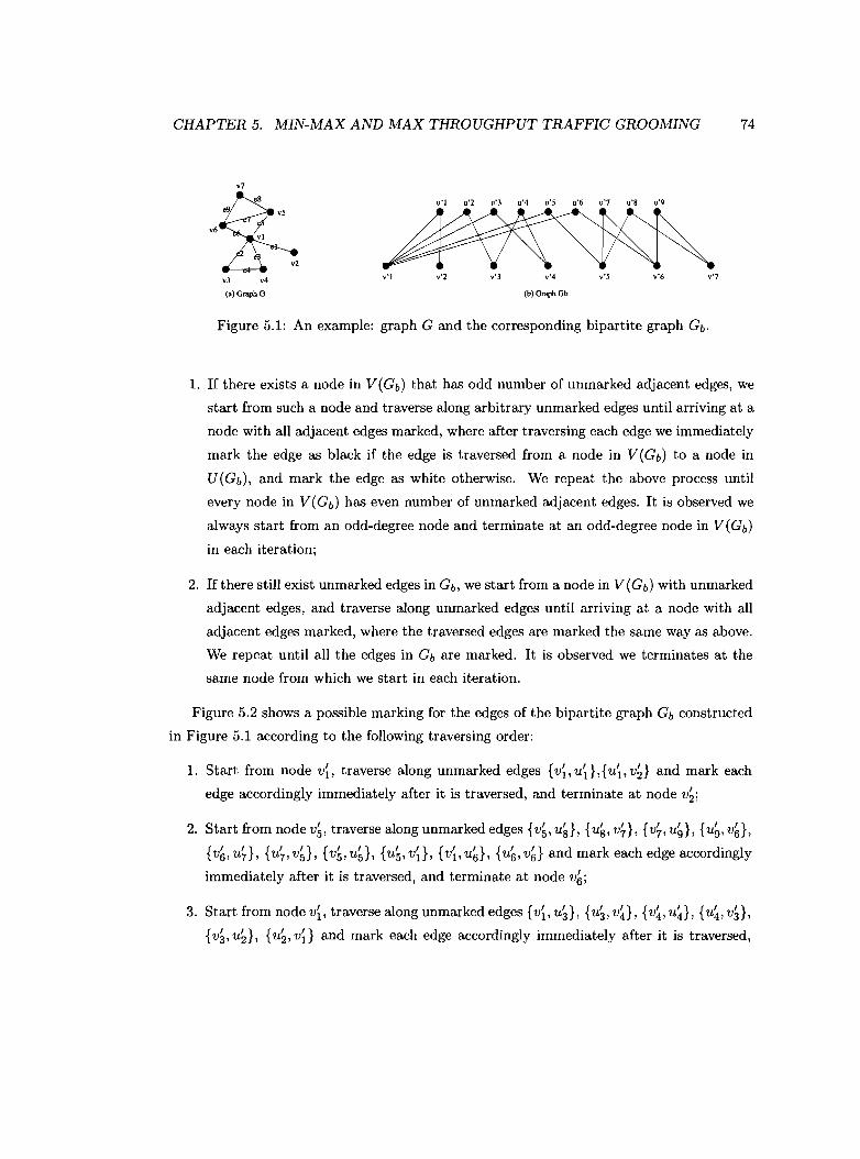
CHAPTER 5. MIN-MAX AND MAX THROUGHPUT TRAFFIC GROOMING 74
v7
u'l u'2 u'3 u'4 u'5 u'6 u'7 u'S u'9
v6
v3 v4 v'l v'2 v'] v'4 v'5 v'6 v'7
<aJ GIlIph G (b) Graph Gb
Figure 5.1: An example: graph G and the corresponding bipartite graph Gb'
1. If there exists a node in V(Gb) that has odd number of unmarked adjacent edges, we
start from such a node and traverse along arbitrary unmarked edges until arriving at a
node with all adjacent edges marked, where after traversing each edge we immediately
mark the edge as black if the edge is traversed from a node in V(Gb) to a node in
U(Gb), and mark the edge as white otherwise. We repeat the above process until
every node in V(Gb ) has even number of unmarked adjacent edges. It is observed we
always start from an odd-degree node and terminate at an odd-degree node in V(Gb)
in each iteration;
2. If there still exist unmarked edges in Gb, we start from a node in V (Gb) with unmarked
adjacent edges, and traverse along unmarked edges until arriving at a node with all
adjacent edges marked, where the traversed edges are marked the same way as above.
We repeat until all the edges in Gb are marked. It is observed we terminates at the
same node from which we start in each iteration.
Figure 5.2 shows a possible marking for the edges of the bipartite graph Gb constructed
in Figure 5.1 according to the following traversing order:
1. Start from node v~, traverse along unmarked edges {v~,uD,{u~,v~} and mark each
edge accordingly immediately after it is traversed, and terminate at node v~;
2. Start from node v~, traverse along unmarked edges {v~, Ug}, {Ug, v~}, {v~, u~}, {u~, v~},
{v~,u~}, {u~,v~}, {v~,u~}, {u~,vD, {v~,u~}, {u~,v~} and mark each edge accordingly
immediately after it is traversed, and terminate at node v~;
3. Start from node v~, traverse along unmarked edges {v~, u~}, {u~, v~}, {v~, u~}, {u~, v~},
{v3' u;}, {u;, vD and mark each edge accordingly immediately after it is traversed,
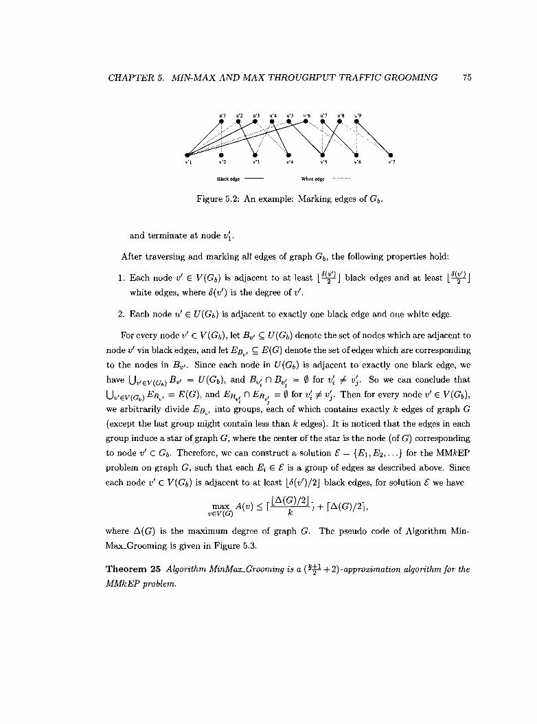
CHAPTER 5. MIN-MAX AND MAX THROUGHPUT TRAFFIC GROOMING 75
u'l u'2 u') u'4 u'S u'6 u'7 u'S
v'' v'3
Black edge --
v'4 v'5
While edge
v'6 v'7
Figure 5.2: An example: Marking edges of Gb.
and terminate at node vi.
After traversing and marking alI edges of graph Gb, the following properties hold:
<l(v' ) Mv' \1. Each node v' E V(Gb) is adjacent to at least l 2 J black edges and at least lT Jwhite edges, where 15(v') is the degree of v'.
2. Each node u' E U(Gb) is adjacent to exactly one black edge and one white edge.
For every node v' E V(Gb), let BVI ~ U(Gb) denote the set of nodes which are adjacent to
node v' via black edges, and let EBvl ~ E(G) denote the set of edges which are corresponding
to the nodes in BV" Since each node in U(Gb) is adjacent to exactly one black edge, we
have UV/EV(Gb) BVI = U(Gb), and B v: n B vj = 0 for v~ f:. vi. So we can conclude that
UV/EV(Gb) EBvl = E(G), and EBvl n EBvl = 0 for v~ f:. vi. Then for every node v' E V(Gb),• 1
we arbitrarily divide EBvl into groups, each of which contains exactly k edges of graph G
(except the last group might contain less than k edges). It is noticed that the edges in each
group induce a star of graph G, where the center of the star is the node (of G) corresponding
to node v' E Gb. Therefore, we can construct a solution £: = {E l , E2,"'} for the MMkEP
problem on graph G, such that each Ei E £: is a group of edges as described above. Since
each node v' E V(Gb) is adjacent to at least l15(v' )/2J black edges, for solution £: we have
max A(v) ~ rl~(~)/2J 1+ r~(G)/21,vEV(G)
where ~(G) is the maximum degree of graph G. The pseudo code of Algorithm Min
Max_Grooming is given in Figure 5.3.
Theorem 25 Algorithm MinMax_Grooming is a (k!l +2)-approximation algorithm for the
MMkEP problem.
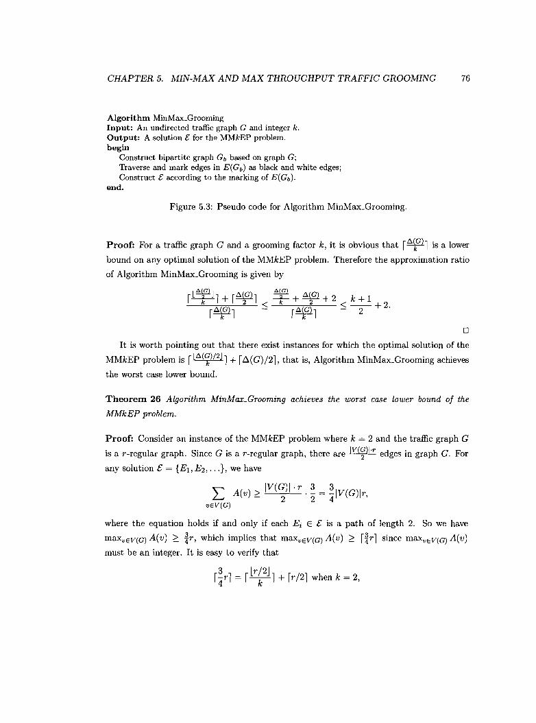
CHAPTER 5. MIN-MAX AND MAX THROUGHPUT TRAFFIC GROOMING 76
Algorithm MinMax_GroomingInput: An undirected traffic graph G and integer k.Output: A solution [ for the MMkEP problem.begin
Construct bipartite graph Gb based on graph G;Traverse and mark edges in E(Gb ) as black and white edges;Construct [ according to the marking of E(Gb)'
end.
Figure 5.3: Pseudo code for Algorithm MinMaLGrooming.
Proof: For a traffic graph G and a grooming factor k, it is obvious that r~~G)l is a lower
bound on any optimal solution of the MMkEP problem. Therefore the approximation ratio
of Algorithm MinMIDcGrooming is given by
o
It is worth pointing out that there exist instances for which the optimal solution of the
MMkEP problem is r l~(~)/2J l + r~(G) /2l, that is, Algorithm MinMaLGrooming achieves
the worst case lower bound.
Theorem 26 Algorithm MinMax_Grooming achieves the worst case lower bound of the
MMkEP problem.
Proof: Consider an instance of the MMkEP problem where k = 2 and the traffic graph G
is a r-regular graph. Since G is a r-regular graph, there are 1V(~)I·r edges in graph G. For
any solution £ = {EI, E2 , .. . }, we have
L A(v) 2: IV(~)I' r . ~ = ~1V(G)lr,vEV(G)
where the equation holds if and only if each Ei E £ is a path of length 2. So we have
maXvEV(G) A(v) 2: ~r, which implies that maXvEV(G) A(v) 2: r~rl since maXvEV(G) A(v)
must be an integer. It is easy to verify that
r~rl = rlr~2Jl + rr/2l when k = 2,
CHAPTER 5. MIN-MAX AND MAX THROUGHPUT TRAFFIC GROOMING 77
hence Algorithm MinMaJLGrooming achieves the worst case lower bound. 0
The bipartite graph construction and the edge traversing/marking procedure can be
done in O(IE(G)I) time, and the solution based on the marking of E(Gb) can be obtained
in O(IE(G)I) time as well. So Algorithm MinMax_Grooming runs in O(IE(G)I) time, which
is linear in the size of the input graph.
5.2.3 Special case: all-to-all traffic pattern
For the all-to-all traffic pattern, the traffic graph is a complete graph. We consider a
complete traffic graph K n containing n nodes.
A lower bound
We first prove a lower bound for the MMkEP problem on an arbitrary traffic graph.
Theorem 27 For a traffic graph G, ~~N]t is a lower bound on optimal solutions for the
MMkEP problem.
Proof: It is noticed that the minimum value of L:vEV(G) A(v) is achieved if we can partition
G into cliques, each of which contains exactly k edges. We also know that a clique of k
edges contains ~+l nodes. Therefore we have
" A(v) > /E(G)I . v'8k+T + 1L.J - k 2'
VEV(G)
and thusmax A(v) > IE(G)I . v'8k+T + 1 > v'2/E (G)I.
vEV(G) - IV(G)I· k 2 IV(G)Iv'ko
Corollary 28 For complete graph K n , ~ is a lower bound on optimal solutions for the
MMkEP problem.
For the case that grooming factor k = 2, since K n is a regular graph as well, the proof
of Theorem 26 shows that Algorithm MinMax_Grooming achieves the optimal solution. In
the following we assume that k ~ 3.
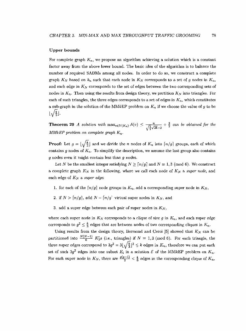
CHAPTER 5. MIN-MAX AND MAX THROUGHPUT TRAFFIC GROOMING 78
Upper bounds
For complete graph K n , we propose an algorithm achieving a solution which is a constant
factor away from the above lower bound. The basic idea of the algorithm is to balance the
number of required SADMs among all nodes. In order to do so, we construct a complete
graph KN based on kn such that each node in KN corresponds to a set of 9 nodes in K n ,
and each edge in K N corresponds to the set of edges between the two corresponding sets of
nodes in K n . Then using the results from design theory, we partition KN into triangles. For
each of such triangles, the three edges corresponds to a set of edges in K n , which constitutes
a sub-graph in the solution of the MMkEP problem on K n if we choose the value of 9 to be
lJj"J.
Theorem 29 A solution with m8.XvEV(Kn ) A(v) < If n + ~ can be obtained for the~v'2k-2
MMkEP problem on complete graph K n .
Proof: Let 9 = lJj"J and we divide the n nodes of K n into fn/g1groups, each of which
contains 9 nodes of K n . To simplify the description, we assume the last group also contains
9 nodes even it might contain less than 9 nodes.
Let N be the smallest integer satisfying N :2: fn/gland N == 1,3 (mod 6). We construct
a complete graph KN in the following, where we call each node of KN a super node, and
each edge of KN a super edge:
1. for each of the fn/gl node groups in K n , add a corresponding super node in KN,
2. if N > fn/gl, add N - fn/gl virtual super nodes in KN, and
3. add a super edge between each pair of super nodes in KN,
where each super node in KN corresponds to a clique of size 9 in K n , and each super edge
corresponds to g2 ::; ~ edges that are between nodes of two corresponding cliques in K n .
Using results from the design theory, Bermond and Ceroi [5] showed that KN can be
partitioned into N(~-I) K~s (i.e., triangles) if N == 1,3 (mod 6). For each triangle, the
three super edges correspond to 3g2 = 3lJj"J2 ::; k edges in K n , therefore we can put each
set of such 3g2 edges into one subset Ei in a solution £ of the MMkEP problem on K n .
For each super node in KN, there are 9(92-1
) < ~ edges in the corresponding clique of K n ,
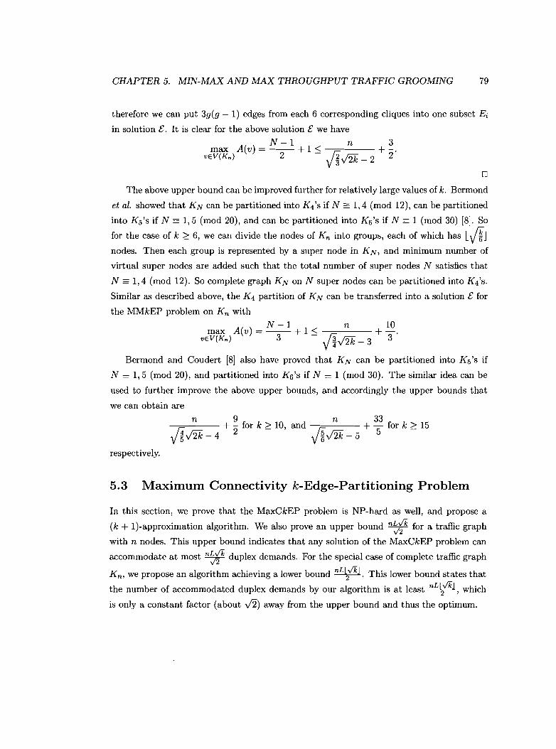
CHAPTER 5. MIN-MAX AND MAX THROUGHPUT TRAFFIC GROOMING 79
therefore we can put 3g(g - 1) edges from each 6 corresponding cliques into one subset Ei
in solution [;. It is clear for the above solution [; we have
N -1 n 3max A(v) = -- + 1 < + -.
vEV(Kn ) 2 - IIv'2k - 2 2
[J
The above upper bound can be improved further for relatively large values of k. Bermond
et al. showed that KN can be partitioned into K 4's if N == 1,4 (mod 12), can be partitioned
into Ks's if N == 1,5 (mod 20), and can be partitioned into K6'S if N == 1 (mod 30) [8]. So
for the case of k 2': 6, we can divide the nodes of K n into groups, each of which has ly1Jnodes. Then each group is represented by a super node in KN, and minimum number of
virtual super nodes are added such that the total number of super nodes N satisfies that
N == 1,4 (mod 12). So complete graph KN on N super nodes can be partitioned into K4'S.
Similar as described above, the K4 partition of KN can be transferred into a solution [; for
the MMkEP problem on K n with
N-l n 10max A(v) = -- + 1 < + -.
vEV(Kn ) 3 - 1fv'2k _ 3 3
Bermond and Coudert [8J also have proved that KN can be partitioned into Ks's if
N == 1,5 (mod 20), and partitioned into K 6 's if N == 1 (mod 30). The similar idea can be
used to further improve the above upper bounds, and accordingly the upper bounds that
we can obtain are
n 9 n 3314 + - for k 2': 10, and 15 + - for k > 15
ygv'2k-4 2 y~v'2k-5 5 -
respectively.
5.3 Maximum Connectivity k-Edge-Partitioning Problem
In this section, we prove that the MaxCkEP problem is NP-hard as well, and propose a
(k + I)-approximation algorithm. We also prove an upper bound nj!! for a traffic graph
with n nodes. This upper bound indicates that any solution of the MaxCkEP problem can
accommodate at most nj!! duplex demands. For the special case of complete traffic graph
K n, we propose an algorithm achieving a lower bound nL~v'kJ. This lower bound states that
the number of accommodated duplex demands by our algorithm is at least nLl2v'kJ, which
is only a constant factor (about J2) away from the upper bound and thus the optimum.
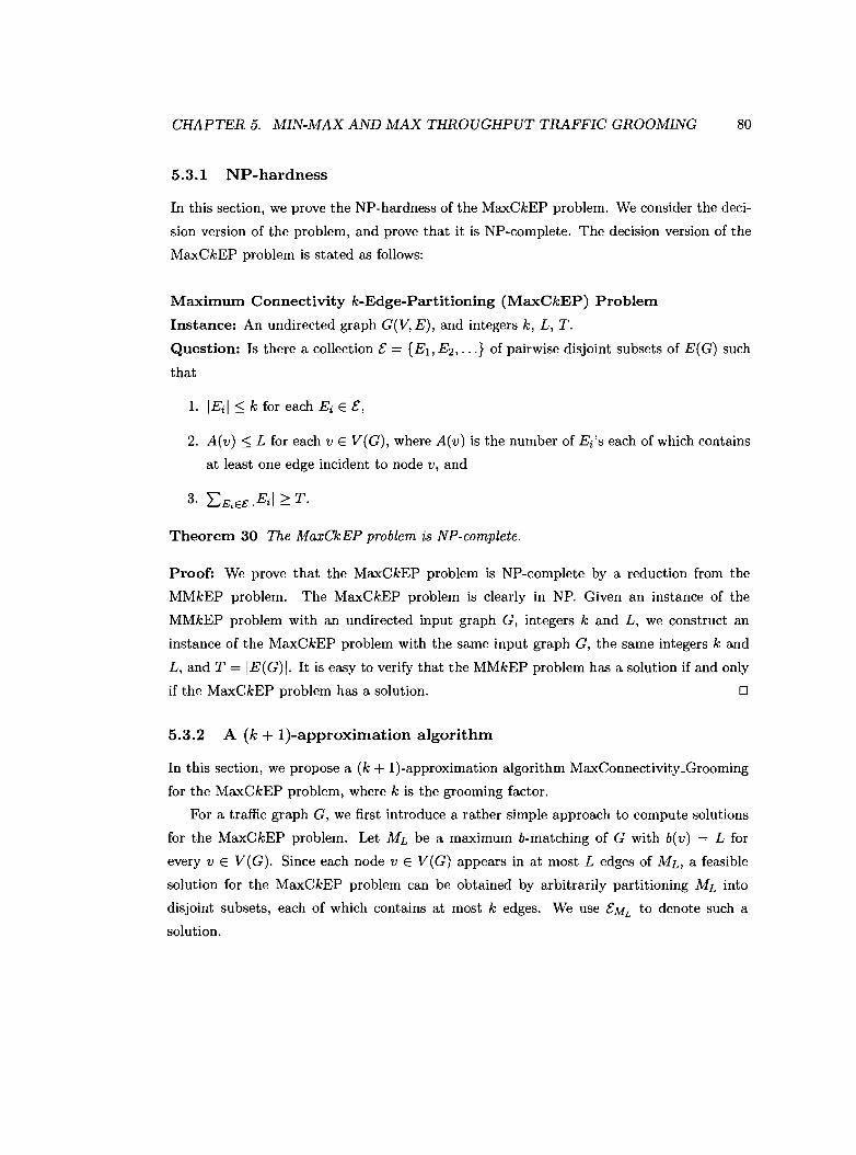
CHAPTER 5. MIN-MAX AND MAX THROUGHPUT TRAFFIC GROOMING 80
5.3.1 NP-hardness
In this section, we prove the NP-hardness of the MaxCkEP problem. We consider the deci
sion version of the problem, and prove that it is NP-complete. The decision version of the
MaxCkEP problem is stated as follows:
Maximum Connectivity k-Edge-Partitioning (MaxCkEP) Problem
Instance: An undirected graph G(V, E), and integers k, L, T.
Question: Is there a collection £ = {El, E2, ... } of pairwise disjoint subsets of E(G) such
that
2. A(v) :::; L for each v E V(G), where A(v) is the number of Ei's each of which contains
at least one edge incident to node v, and
Theorem 30 The MaxCkEP problem is NP-complete.
Proof: We prove that the MaxCkEP problem is NP-complete by a reduction from the
MMkEP problem. The MaxCkEP problem is clearly in NP. Given an instance of the
MMkEP problem with an undirected input graph G, integers k and L, we construct an
instance of the MaxCkEP problem with the same input graph G, the same integers k and
L, and T = IE(G)/. It is easy to verify that the MMkEP problem has a solution if and only
if the MaxCkEP problem has a solution. D
5.3.2 A (k + I)-approximation algorithm
In this section, we propose a (k + I)-approximation algorithm MaxConnectivity_Grooming
for the MaxCkEP problem, where k is the grooming factor.
For a traffic graph G, we first introduce a rather simple approach to compute solutions
for the MaxCkEP problem. Let ML be a maximum b-matching of G with b(v) = L for
every v E V(G). Since each node v E V(G) appears in at most L edges of ML, a feasible
solution for the MaxCkEP problem can be obtained by arbitrarily partitioning M L into
disjoint subsets, each of which contains at most k edges. We use £ML to denote such a
solution.
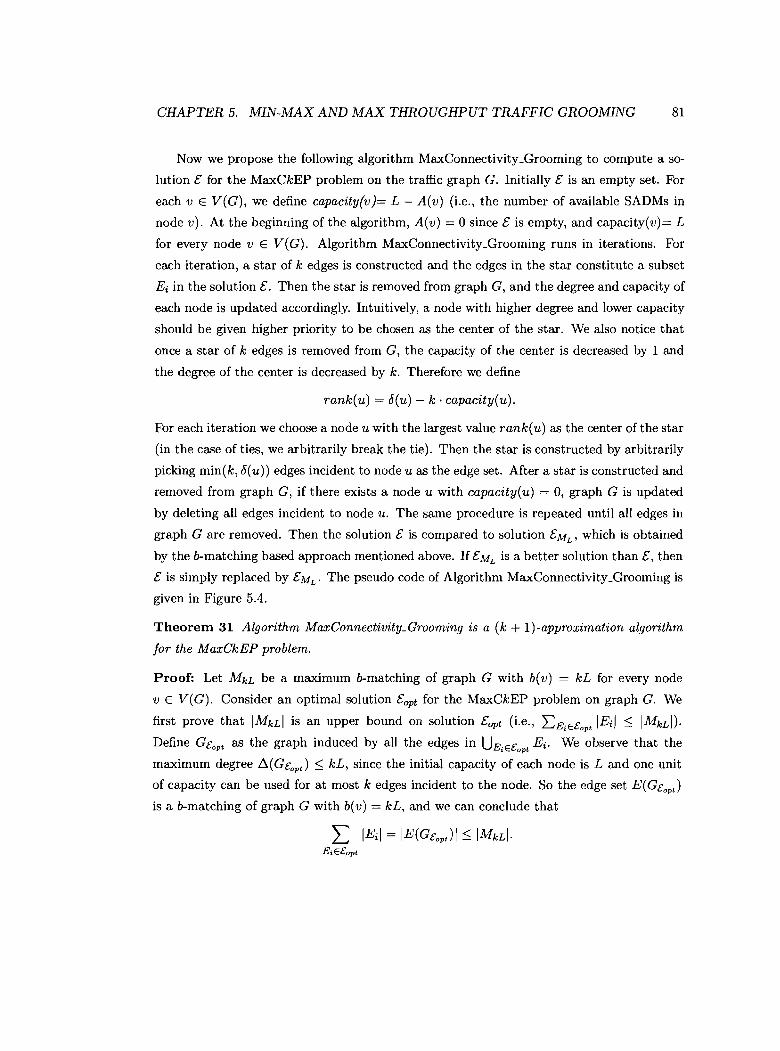
CHAPTER 5. MIN-MAX AND MAX THROUGHPUT TRAFFIC GROOMING 81
Now we propose the following algorithm MaxConnectivity_Grooming to compute a so
lution C for the MaxCkEP problem on the traffic graph G. Initially c is an empty set. For
each v E V(G), we define capacity(v)= L - A(v) (i.e., the number of available SADMs in
node v). At the beginning of the algorithm, A(v) = 0 since c is empty, and capacity(v)= L
for every node v E V(G). Algorithm MaxConnectivity_Grooming runs in iterations. For
each iteration, a star of k edges is constructed and the edges in the star constitute a subset
Ei in the solution c. Then the star is removed from graph G, and the degree and capacity of
each node is updated accordingly. Intuitively, a node with higher degree and lower capacity
should be given higher priority to be chosen as the center of the star. We also notice that
once a star of k edges is removed from G, the capacity of the center is decreased by 1 and
the degree of the center is decreased by k. Therefore we define
rank(u) = o(u) - k· capacity(u).
For each iteration we choose a node u with the largest value rank(u) as the center of the star
(in the case of ties, we arbitrarily break the tie). Then the star is constructed by arbitrarily
picking min(k, o(u)) edges incident to node u as the edge set. After a star is constructed and
removed from graph G, if there exists a node u with capacity(u) = 0, graph G is updated
by deleting all edges incident to node u. The same procedure is repeated until all edges in
graph G are removed. Then the solution c is compared to solution CML
, which is obtained
by the b-matching based approach mentioned above. IfCML is a better solution than C, then
C is simply replaced by CML • The pseudo code of Algorithm MaxConnectivity_Grooming is
given in Figure 5.4.
Theorem 31 Algorithm MaxConnectivity_Grooming is a (k + I)-approximation algorithm
for the MaxCkEP problem.
Proof: Let MkL be a maximum b-matching of graph G with b(v) = kL for every node
v E V(G). Consider an optimal solution copt for the MaxCkEP problem on graph G. We
first prove that IMkLI is an upper bound on solution Copt (i.e., LEiE[opt IEil ~ IMkLI).
Define G[opt as the graph induced by all the edges in UEiE[OPt Ei. We observe that the
maximum degree ~(G[oPt) ~ kL, since the initial capacity of each node is L and one unit
of capacity can be used for at most k edges incident to the node. So the edge set E(G[opJ
is a b-matching of graph G with b(v) = kL, and we can conclude that
L IEil = IE(G[opt)1 ~ IMkLI·EiE[opt
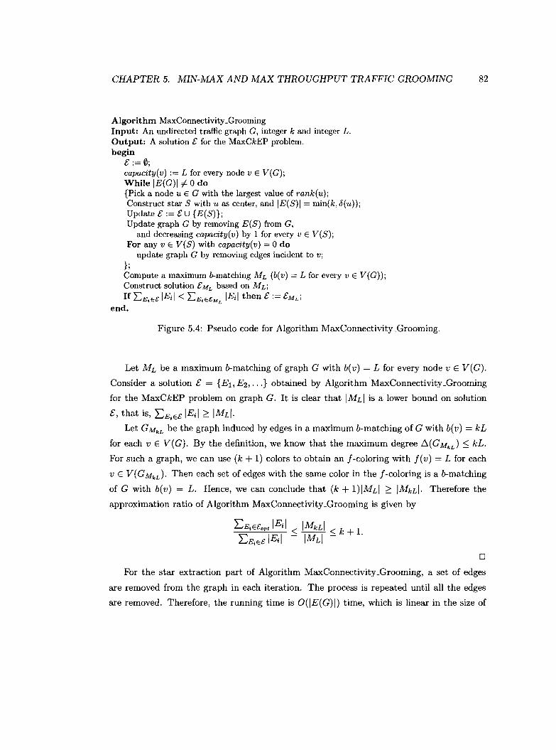
CHAPTER 5. MIN-MAX AND MAX THROUGHPUT TRAFFIC GROOMING 82
Algorithm MaxConnectivity_GroomingInput: An undirected traffic graph G, integer k and integer L.Output: A solution C for the MaxCkEP problem.begin
C :=0;capacity(v) := L for every node v E V(G);While IE(G)I i 0 do{Pick a node u E G with the largest value of rank(u);Construct star S with u as center, and IE(S)I = min(k,<5(u));Update c := c U {E(S)};Update graph G by removing E(S) from G,
and decreasing capacity(v) by 1 for every v E V(S);For any v E V(S) with capacity(v) = 0 do
update graph G by removing edges incident to v;};Compute a maximum b-matching ML (b(v) = L for every v E V(G));Construct solution CML based on M L ;
IfL:EEt:IEil <L:EEt: IEil thenc:=cML;... 't M L
end.
Figure 5.4: Pseudo code for Algorithm MaxConnectivity_Grooming.
Let ML be a maximum b-matching of graph G with b(v) = L for every node v E V(G).
Consider a solution £ = {El, E2, ...} obtained by Algorithm'MaxConnectivity_Grooming
for the MaxCkEP problem on graph G. It is clear that IMLI is a lower bound on solution
£, that is, LE;Et: IEil ::::: IMLI·Let GMkL be the graph induced by edges in a maximum b-matching of G with b(v) = kL
for each v E V(G). By the definition, we know that the maximum degree b.(GMkL ) ~ kL.
For such a graph, we can use (k + 1) colors to obtain an f -coloring with f (v) = L for each
v E V (GM kL ). Then each set of edges with the same color in the f -coloring is a b-matching
of G with b(v) = L. Hence, we can conclude that (k + l)IMLI ::::: IMkLI. Therefore the
approximation ratio of Algorithm MaxConnectivity_Grooming is given by
o
For the star extraction part of Algorithm MaxConnectivity_Grooming, a set of edges
are removed from the graph in each iteration. The process is repeated until all the edges
are removed. Therefore, the running time is O(IE(G)I) time, which is linear in the size of
CHAPTER 5. MIN-MAX AND MAX THROUGHPUT TRAFFIC GROOMING 83
the input graph. While for the part to compute a maximum b-matching with b(v) = L, the
running time is JLJV(G)IIE(G)I [23]. Therefore, Algorithm MaxConnectivity_Grooming
runs in JLJV(G)IIE(G)I time.
5.3.3 Special case: all-to-all traffic pattern
In this section, we study the MaxCkEP problem on complete traffic graph K n containing n
nodes, each of which has a capacity of L initially.
An upper bound
We first prove an upper bound for the MaxCkEP problem on an arbitrary traffic graph, in
which each node has a capacity L initially.
Theorem 32 For a traffic graph G, IV(Gjv'k is an upper bound on optimal solutions for
the MaxCkEP problem.
Proof: For graph G, the total capacity over all nodes is JV(G)IL. It is observed that a
clique of k edges consumes the minimum units of capacity, which is i8kf+l, among all
sub-graphs of k edges. Therefore an upper bound on optimal solutions is
IV(G)IL . k < JV(G)IL . k = IV(G)ILVk~+1 ~ V2
2 2
o
Corollary 33 For complete graph K n , n~ is an upper bound on optimal solutions for the
MaxCkEP problem.
A lower bound
For complete graph K n , we propose an algorithm achieving a solution which is a constant
factor away from the above upper bound. We first prove the following lemma about a
complete graph K 2m with even number 2m of nodes.
Lemma 34 The edge set of complete graph K 2m can be partitioned into (2m - 1) pairwise
disjoint subsets, such that each subset is a perfect matching of K 2m .
CHAPTER 5. MIN-MAX AND MAX THROUGHPUT TRAFFIC GROOMING 84
Proof: It is known that an edge coloring of K2m can be obtained using 2m - 1 colors [22].
We notice that each set of edges with the same color is a matching of K 2m , so the number
of edges with the same color is at most m for every color. The total number of edges in
K2m is m(2m - 1), therefore it must be the case that the number of edges with the same
color is exactly m for each color, which implies that each set of edges with the same color
is a perfect matching of K 2m- 0
The basic idea of the algorithm is still to balance the use of SADMs among all nodes.
In order to do so, we construct a complete graph K N based on kn such that each node in
KN corresponds to a set of 9 nodes in K n , and each edge in KN corresponds to the set
of edges between the two corresponding sets of nodes in K n . Then we partition KN into
perfect matchings according to Lemma 34. Each edge in the matchings corresponds to a set
of edges in K n , which constitutes a sub-graph in the solution of the MaxCkEP problem on
K n if we choose the value of 9 to be lv'kJ.
Theorem 35 A solution [; with LE;E£ IEil > nL~.jkJ can be obtained for the MaxCkEP
problem on complete graph K n .
Proof: Let 9 = lv'kJ and we divide the n nodes of K n into rn/91groups, each of which
contains 9 nodes of K n • To simplify the description, we assume that the last group also
contains 9 nodes even it might contain less than 9 nodes.
Let N = rn/91, and we construct a complete graph KN, where we call each node of KN
a super node, and each edge of K N a super edge:
1. for each of the rn/91node groups in K n , add a corresponding super node in KN, and
2. add a super edge between each pair of super nodes in KN,
where each super node in KN corresponds to a clique of size 9 in K n , and each super edge
corresponds to g2 ::; k edges that are between nodes of two corresponding cliques in K n .
We assume that N is even, since otherwise we can add one virtual super node and some
corresponding virtual super edges.
According to Lemma 34, the edge set of KN can be partitioned into (N - 1) perfect
matchings. Since every super edge in each perfect matching corresponds to g2 ::; k edges of
K n , we can arbitrarily pick L perfect matchings, and construct solution [; = {El, E2, ... }
such that each Ei E [; consists of edges (of K n ) corresponding to a super edge in the L
CHAPTER 5. MIN-MAX AND MAX THROUGHPUT TRAFFIC GROOMING 85
perfect matchings of K N. Therefore
'" IE-I =L· N .g2 =L. fn/gl .g2 > nLg = nLlVkJLJ t 2 2 - 2 2'
EiEC
o
The lower bound obtained above is based on two assumptions: the number of nodes in
the last group is g, and N is an even integer. It can be easily verified that the difference
will only be a constant value even if we do not make the assumptions.
5.4 Empirical results
In this section, we will conduct extensive simulations to evaluate the practical perfor
mances of our algorithms by comparing to the corresponding worst case performances and
lower/upper bounds. We implemented Algorithm MinMax_Grooming and Algorithm Max
Connectivity_Grooming to validate their performances on randomly generated traffic graphs.
In generating graphs, we specify the number n of nodes and density ratio d that is used to
calculate the number m = n l+d of edges. A graph G of m edges and n nodes is generated
by randomly connecting m pairs of nodes among all n(n - 1)/2 possible pairs. Figure 5.5
shows the empirical results of Algorithm MinMax_Grooming on graphs of 36 nodes with
density ratio d = 0.6, where for each value of grooming factor k, we collect the results from
100 randomly generated traffic graphs and compute the average value. The lower bound
we used for measuring Algorithm MinMax_Grooming is f~~G) 1, which is mentioned in The
orem 25. Figure 5.8 shows the empirical results of Algorithm MaxConnectivity_Grooming
on graphs of 36 nodes with density ratio d = 0.6 and grooming factor k = 4, where for
each value of capacity L, we collect the results from 100 randomly generated traffic graphs
and compute the average value. The upper bound we used for measuring Algorithm Max
Connectivity_Grooming is IMkLI, which is mentioned in Theorem 31. We observe that the
experimental performances of both algorithms are considerably better than the worst case
performances proved in Section 5.2.2 and Section 5.3.2. In addition, the results show that
the solution obtained by Algorithm MinMax_Grooming is close to the corresponding lower
bound, and the solution obtained by Algorithm MaxConnectivity_Grooming is close to the
corresponding upper bound. Simulations are conducted on graphs with different parameter
settings as well, and the results present similar characteristics (see Figure 5.6, Figure 5.7,
Figure 5.9, and Figure 5.10 for other representative results).

CHAPTER 5. MIN-MAX AND MAX THROUGHPUT TRAFFIC GROOMING 86
AIgoriltlm MinMax Grooming0
-
5//'~
~--////~,,-------0
5
1-pro..bl. wont ca.. penormanc"I0 --+-- experimental performanca
---t- Klwer bound
5
o3 6 7
grooming factor k10
Figure 5.5: Performance of Algorithm MinMax_Grooming for n = 36 and d = 0.6 .
5.5 Summary
In this chapter, using novel graph partitioning approaches, we studied traffic grooming for
both the problem to minimize the maximum number of SADMs over all network nodes,
and the problem to maximize the number of accommodated traffic demands subject to
limited number of SADMs. We proved both problems are NP-hard for the UPSR network
with unitary duplex traffic demands, and proposed an approximation algorithm for each
problem. We also studied the all-to-all traffic pattern, and proposed algorithms achieving
solutions only constant factors away from the optimal ones for both problems. For the
future work, it is interesting to further narrow the gap between the lower bound and the
upper bound for both the MMkEP problem and the MaxCkEP problem. Intuitively, a good
approach for both problems should balance the usage of SADMs among all nodes. As we
did in Algorithm MinMax_Grooming and Algorithm MaxConnectivity_Grooming, stars are
extracted from the traffic graph in iterations to achieve such a balance. However, when
the degrees of all nodes tend to be uniform (the extreme case is that all nodes have the
same degree, i.e., the traffic graph is a regular graph), extracting a star each time from
the traffic graph might not be good enough. A possible approach could be to extract a
regular sub-graph for each iteration from the traffic graph. Therefore, the ideal solution for
both problems should also take the structure of the traffic graph into account, and use a
combination of star and other topologies for extracting sub-graphs.
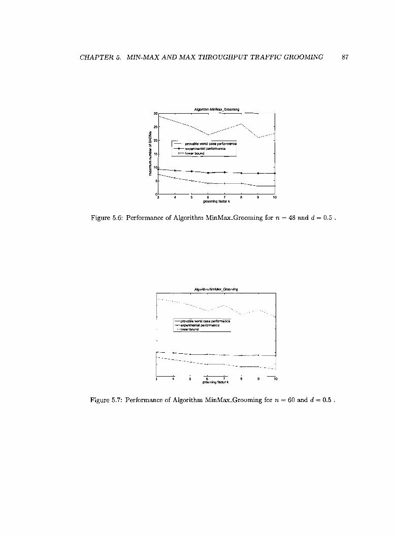
CHAPTER 5. MIN-MAX AND MAX THROUGHPUT TRAFFIC GROOMING 87
Algorithm MinMax_Grooming30r--~--~-=--~--="-----::""'---~----,
1------.• 25 ~~ ~~----~~20 ~ ~-_ •.•
'0 r-- provable worst case performsn1.M ------- experimental performanceE 15 --t-" lower bound
~E110r--.~ .......__~ -l
E sr-----------.....--+-----+----+----L
°3L--~--·~--6~----'-7--~--~---.J10
grooming factor k
Figure 5.6: Performance of Algorithm MinMrocGrooming for n = 48 and d = 0.5
1
- prova~e worst case P8rfonnanci--expenmentBl performance----<---lower bound
~_.-I-_~
-------------- -
6 7grooming factor k
10
Figure 5.7: Performance of Algorithm MinMrocGrooming for n = 60 and d = 0.5 .
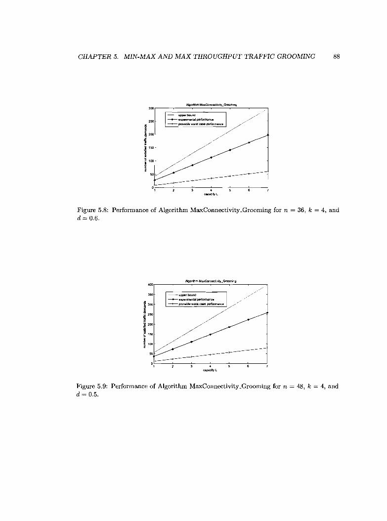
CHAPTER 5. MIN-MAX AND MAX THROUGHPUT TRAFFIC GROOMING 88
AIgor1thm Max-Conneclivity-Grooming3oor---~--'-,---~----'-''-----'--'----~--/l
-- upper bound
250 --+-- uperimen1a1 performance---+-- provable wont case performance //
~ //
i 200 ///
~ /11150- /
i /°100- /I /~ 50~
°1'----:-------7--~4----~--~--
capacIty L
Figure 5.8: Performance of Algorithm MaxConnectivity_Grooming for nd= 0.6.
AIgorilhm MaxConnecUvity_Grooming4oor---~--~--~---'---~---",
36, k = 4, and
350
~ 300
i~ 250
~11 200
!~15O~~ 100
50
-- upper bound
---+- experimental performance---+-- provable worst caee performance ./
,/'///
////
/~O,L--~'-----7---~4~---:-------7------:'
capacity L
Figure 5.9: Performance of Algorithm MaxConnectivity_Grooming for n = 48, k = 4, andd= 0.5.

CHAPTER 5. MIN-MAX AND MAX THROUGHPUT TRAFFIC GROOMING 89
Algoliltlrn MaxConnectivitLGrooming500r--~--":""---~----=:::"-~-=--~--,,""
/
"
<capacity L
-- upper bound_____ experimental perlormance //
~ provable ,"0'" cue ..do""aneo //
,,/
/",
//o'------~--~--~--~--~---.J
1
<50
.<00
j 350
~ 300
~250
i 200'l;
.li '50~c 100
Figure 5.10: Performance of Algorithm MaxConnectivity_Grooming for n = 60, k = 4, andd = 0.5.
Chapter 6
Traffic grooming in BLSR networks
As another important architecture for SONET/WDM ring networks, BLSR is widely used
in optical network design as well. Compared to UPSR networks, the routing of a traffic
demand in BLSR networks is not unique. Traffic demands can be routed in either clockwise
or counter-clockwise direction. Generally speaking, this flexibility in routing makes the
traffic grooming problem in BLSR networks more complicated than UPSR networks. As
mentioned in Chapter 2, the traffic grooming problem in BLSR network is usually solved
by a two-step approach: the first step is to generate primitive cycles, and the second step
is to groom primitive cycles into wavelength channels. The two steps are not completely
independent, therefore it can not be guaranteed that the number of used SADMs is optimal
even if the optimal solution can be achieved for each step individually. For the traffic
grooming problem in BLSR networks, we adopt the two-step approach, and use previous
algorithms to obtain the solution for the first step. From now on, we assume that the solution
for the first step is available unless otherwise stated, and focus on solving the second step.
6.1 Definitions and problem formulations
We formulate the traffic grooming problems into hypergraph partitioning problems. A
hypergraph H(V, EH) of n nodes and m hyperedges is a graph with node set V and hyperedge
set EH = {el, e2,"" em}, where each hyperedge ei is a subset of V with ni (ni ~ 2) nodes.
For the two-step approach to solve the traffic grooming in BLSR networks, once the
solution for the first step is given, we can construct a traffic hypergraph as follows: the node
set represents the set of network nodes in the BLSR network; there is a hyperedge in the
90
CHAPTER 6. TRAFFIC GROOMING IN BLSR NETWORKS 91
hypergraph corresponding each primitive cycle, where the set of nodes in a hyperedge is the
set of network nodes as the sources or destinations of the traffic demands groomed in the
corresponding primitive cycle. We will formulate the traffic grooming problems using this
hypergraph model.
Similar as the k-Edge-Partitioning Problem, the traffic grooming problem to minimize
the total number of SADMs in BLSR networks can be formulated as the following parti
tioning problem on the traffic hypergraph:
k-Edge-Partitioning of Hypergraph Problem (kEPH)
Instance: A traffic hypergraph H(V, E) and integer k::; IE(H)I.
Objective: Partition the hyperedge set E(H) into a collection of subsets [; = {EI, E2, ... }
(where UiEi = E(H) and Ep n Eq = 0 for P 1: q), such that IEil ::; k for each Ei E [;
and LEiE£IViI is minimized, where Vi is the set of nodes in the sub-hypergraph induced by
hyperedge set E i .
Similar as the Min-Max k-Edge-Partitioning Problem, the Min-Max traffic grooming
problem in BLSR networks can be formulated as the following Min-Max k-Edge-Partitioning
of Hypergraph problem (MMkEPH):
Min-Max k-Edge-Partitioning of Hypergraph Problem (MMkEPH)
Instance: A traffic hypergraph H(V,E) and integer k::; jE(H)I.
Objective: Partition the hyperedge set E(H) into a collection of pairwise disjoint subsets
[; = {EI' E2, ... } such that lEi I ::; k for each Ei E [;. The objective is to minimize the value
of m8.XvEV(H) A(v), where A(v) is the number of Ei's each of which contains at least one
hyperedge incident to node v.
Similar as the Maximum Connectivity k-Edge-Partitioning Problem, the Maximum
Throughput traffic grooming problem in BLSR networks can be formulated as the following
Maximum Connectivity k-Edge-Partitioning of Hypergraph problem (MaxCkEPH):
Maximum Connectivity k-Edge-Partitioning of Hypergraph Problem (MaxCkEPH)
Instance: A traffic hypergraph H(V, E), an integer k::; IE(H)I and an integer L.
Objective: Find a collection [; = {EI' E2,"'} of pairwise disjoint subsets of E(H) such
that IEil ::; k for each Ei E [; and A(v) ::; L for each v E V(H), where A(v) is the number
CHAPTER 6. TRAFFIC GROOMING IN BLSR NETWORKS 92
of E;'s each of which contains at least one hyperedge incident to node v. The objective is
to maximize LEiEE IE;I.Since all the three corresponding graph partitioning problems are NP-hard, it can be
easily proved that the following theorem holds.
Theorem 36 The kEPH problem, the MMkEPH problem, and the MaxCkEPH problem
are NP-hard.
Proof: Trivial.
6.2 Algorithms
o
In this section, we will focus on designing algorithms for the MMkEPH problem and the
MaxCkEPH problem. As to the kEPH problem, it has been well studied in previous work
which uses the hypergraph partitioning formulation implicitly.
6.2.1 Algorithms for the MMkEPH problem
In this section, we propose a simple greedy algorithm MinMax_Hyper for the MMkEPH
problem. The basic idea of this algorithm is to balance the SADM usage among all the
nodes in the network. The algorithm runs in iterations. For each iteration, a node v with
the maximum degree is chosen. Then arbitrary k hyperedges incident to v are chosen to
form a sub-hypergraph and deleted from the hypergraph, and accordingly the degrees of
the affected nodes in the hypergraph are updated. The same process is repeated until every
hyperedge is deleted from the hypergraph and included into some sub-hypergraph. During
each iteration, we also maintain a variable L(v) for each node v to denote the number
of sub-hypergraphs containing at least one hyperedge incident to v (i.e., L(v) denotes the
number of consumed SADMs at node v) so far. Thus if there is a tie when comparing the
degrees of the nodes, we choose the node with the largest L(v) to break the tie (we will
arbitrarily break the tie if it still exists). Eventually, all the sub-hypergraphs will constitute
a hypergraph partition, which gives a solution for the MMkEPH problem. The pseudo code
of Algorithm MinMax_Hyper is given in Figure 6.1. We will show the empirical results in
Section 6.3.
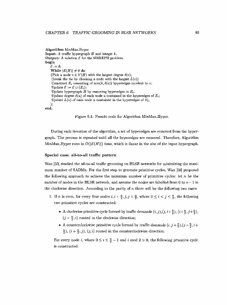
CHAPTER 6. TRAFFIC GROOMING IN BLSR NETWORKS
Algorithm MinMaxJIyperInput: A traffic hypergraph H and integer k.Output: A solution E: for the MMkEPH problem.begin
E::= 0;While IE(H)I =I 0 do{Pick a node v E V(H) with the largest degree 8(v);(break the tie by choosing a node with the largest L(v))Construct E; consisting of min(k, 8(v)) hyperedges incident to v;Update E: := E: U {E;};Update hypergraph H by removing hyperedges in E;;Update degree 8(u) of each node u contained in the hyperedges of E;;Update L(u) of each node u contained in the hyperedges of E;;
};end.
Figure 6.1: Pseudo code for Algorithm MinMax_Hyper.
93
During each iteration of the algorithm, a set of hyperedges are removed from the hyper
graph. The process is repeated until all the hyperedges are removed. Therefore, Algorithm
MinMax-Hyper runs in O(IE(H)I) time, which is linear in the size of the input hypergraph.
Special case: all-to-all traffic pattern
Wan [50J studied the all-to-all traffic grooming on BLSR networks for minimizing the maxi
mum number of SADMs. For the first step to generate primitive cycles, Wan [50J proposed
the following approach to achieve the minimum number of primitive cycles: let n be the
number of nodes in the BLSR network, and assume the nodes are labelled from °to n - 1 in
the clockwise direction. According to the parity of n there will be the following two cases:
1. If n is even, for every four nodes i, i + ~,j,j + ~, where °~ i < j ~ ~, the following
two primitive cycles are constructed:
• A clockwise primitive cycle formed by traffic demands (i,j),(j, i+~), (i+~,j+~),
(j + ~,i) routed in the clockwise direction;
• A counterclockwise primitive cycle formed by traffic demands (i,j + ~),(j +~, i+
~), (i + ~,j), (j, i) routed in the counterclockwise direction.
For every node i, where °~ i ~ ~ - 1 and i mod 2 == 0, the following primitive cycle
is constructed:
CHAPTER 6. TRAFFIC GROOMING IN BLSR NETWORKS 94
• A clockwise primitive cycle formed by traffic demands (i, i + ~), (i +~, i) routed
in the clockwise direction.
For every node i, where 0 ~ i ~ ~ - 1 and i mod 2 == 1, the following primitive cycle
is constructed:
• A counterclockwise primitive cycle formed by traffic demands (i, i + ~), (i +~, i)
routed in the counterclockwise direction.
Therefore the total number of primitive cycles is 2(t) + ~ = ~2, where there are r~21
primitive cycles in one direction and l ~2 J in the other direction.
2. If n is odd, for every four nodes i,i + r~l,j,j + r~l, where 0 ~ i < j < l~J, the
following two primitive cycles are constructed:
• A clockwise primitive cycle formed by traffic demands (i,j),(j, i + r~l), (i +r~l,j + r~l), (j + r~l,i) routed in the clockwise direction;
• A counterclockwise primitive cycle formed by traffic demands (i,j + r~l), (j +r~1, i + r~1), (i + r~1, j), (j, i) routed in the counterclockwise direction.
For every node i, where 0 ~ i < l~J, the following two primitive cycles are constructed:
• A clockwise primitive cycle formed by traffic demands (i, l~J), (l~ J, i + r~1),(i + r~1, i) routed in the clockwise direction;
• A counterclockwise primitive cycle formed by traffic demands (i,i + r~l), (i +r~l, l~J), (l~J,i) routed in the counterclockwise direction.
Therefore the number of primitive cycles is (l ~ J) + l~J = n2
s-1 in each of the clockwise
and counterclockwise directions.
Based on the above construction of primitive cycles, we can construct a traffic hypergraph
and use algorithm MinMaxJIyper to solve the MMkEPH problem. However, due to the
special scheme of constructing primitive cycles, a better approach can be used to compute
the solution. We will describe the case for n being even in the following, and the case for n
being odd can be solved in a similar way.
If n is even, we assume that n = 2m without loss of generality. We construct a complete
graph K m with m nodes as follows: each node i in K m represents a node pair (i, i + ~) in

CHAPTER 6. TRAFFIC GROOMING IN BLSR NETWORKS 95
the BLSR; the edge between node i and j in K m represents the two primitive cycles formed
by traffic demands (i,j),(j,i + ~), (i + ~,j + ~), (j + ~,i) in the clockwise direction and
traffic demands (i, j + ~), (j + ~, i + ~), (i + ~, j), (j, i) in the counterclockwise direction. It
is also noticed that there is a primitive cycle between each node pair (i, i + ~), and there are
~ primitive cycles in total for each of the clockwise and counterclockwise directions. We
use a hidden edge to denote each pair of such primitive cycles in the complete graph K m .
For the complete graph K m , we can use the same algorithm described in Section 5.2.3 to
groom the edges of K m , and use one extra SADM at each node to groom the hidden edges.
Therefore, we have the follow corollary based on Theorem 29.
Corollary 37 A solution with maxv A(v) ~ If m + ~ can be obtained for the Min-MaxJv'2k-2 .
grooming of all-to-all traffic in BLSR networks.
As well, the solution can be improved further to Nil + 1 ~ n + g for k > 6Ifv'2k-3 3 -,
and VI n + ~1 for k 2: 10, and Ii n + ¥ for k 2: 15, as derived in Section 5.2.3.sv'2k-4 6v'2k-5
6.2.2 Algorithms for the MaxCkEPH problem
It is observed that Algorithm MaxConnectivity_Grooming proposed in Section 5.3.2 can
be directly applied to solve the Maximum Connectivity k-Edge-Partitioning of Hypergraph
problem. However, the theoretical analysis of the performance guarantee uses the results of
the maximum b-matching of graphs, which are not known for hypergraphs. Therefore, the
approximation ratio of Algorithm MaxConnectivity_Grooming can not be preserved for the
MaxCkEPH problem.
Special case: all-to-all traffic pattern
As illustrated in Section 6.2.1, we can use a complete graph with some hidden edges to denote
the primitive cycles constructed by the approach in [50]. For the Maximum Throughput
traffic grooming problem, the algorithm proposed in Section 5.3.3 can be used directly to
achieve the same performance. Based on Theorem 35, we have the follow corollary for the
Maximum Throughput grooming of all-to-all traffic in BLSR networks.
Corollary 38 A solution £ with L:EiE£ IEil 2: mL~VkJ can be obtained for the Maximum
Throughput grooming of all-to-all traffic in BLSR networks.
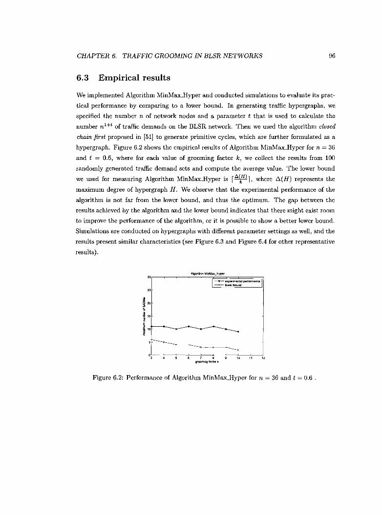
CHAPTER 6. TRAFFIC GROOMING IN BLSR NETWORKS
6.3 Empirical results
96
We implemented Algorithm MinMa)cHyper and conducted simulations to evaluate its prac
tical performance by comparing to a lower bound. In generating traffic hypergraphs, we
specified the number n of network nodes and a parameter t that is used to calculate the
number nl+t of traffic demands on the BLSR network. Then we used the algorithm closed
chain first proposed in [51] to generate primitive cycles, which are further formulated as a
hypergraph. Figure 6.2 shows the empirical results of Algorithm MinMaJcHyper for n = 36
and t = 0.6, where for each value of grooming factor k, we collect the results from 100
randomly generated traffic demand sets and compute the average value. The lower bound
we used for measuring Algorithm MinMaxJIyper is r~1H) 1, where Do (H) represents the
maximum degree of hypergraph H. We observe that the experimental performance of the
algorithm is not far from the lower bound, and thus the optimum. The gap between the
results achieved by the algorithm and the lower bound indicates that there might exist room
to improve the performance of the algorithm, or it is possible to show a better lower bound.
Simulations are conducted on hypergraphs with different parameter settings as well, and the
results present similar characteristics (see Figure 6.3 and Figure 6.4 for other representative
results).
Algorilhm MinM8X_Hyper30
25
:I~ 20
l;
j 15~
~ ~i 10e
1
----.- experimental perfonnance--+-- klwer bound
o'--~-~-~-~-~~-~-~--'
3 7 8 10 11 12grooming faClOf k
Figure 6.2: Performance of Algorithm MinMaxJIyper for n = 36 and t = 0.6 .
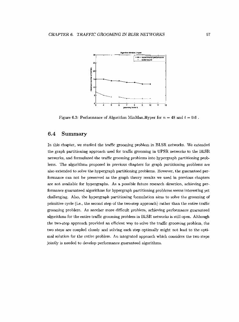
CHAPTER 6. TRAFFIC GROOMING IN BLSR NETWORKS
Algorilhm MinMax_Hyper30,~-~-"--:~-7"=======il
1
expenmental performance I--+- lower bound I
25
°3:-~----=--7-~7'------~8-~-----'1~O-~11-----'---"2
grooming 'acteN' k
Figure 6.3: Performance of Algorithm MinMmcHyper for n = 48 and t = 0.6 .
6.4 Summary
97
In this chapter, we studied the traffic grooming problem in BLSR networks. We extended
the graph partitioning approach used for traffic grooming in UPSR networks to the BLSR
networks, and formulated the traffic grooming problems into hypergraph partitioning prob
lems. The algorithms proposed in previous chapters for graph partitioning problems are
also extended to solve the hypergraph partitioning problems. However, the guaranteed per
formance can not be preserved as the graph theory results we used in previous chapters
are not available for hypergraphs. As a possible future research direction, achieving per
formance guaranteed algorithms for hypergraph partitioning problems seems interesting yet
challenging. Also, the hypergraph partitioning formulation aims to solve the grooming of
primitive cycle (i.e., the second step of the two-step approach) rather than the entire traffic
grooming problem. As another more difficult problem, achieving performance guaranteed
algorithms for the entire traffic grooming problem in BLSR networks is still open. Although
the two-step approach provided an efficient way to solve the traffic grooming problem, the
two steps are coupled closely and solving each step optimally might not lead to the opti
mal solution for the entire problem. An integrated approach which considers the two steps
jointly is needed to develop performance guaranteed algorithms.
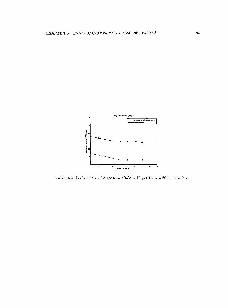
CHAPTER 6. TRAFFIC GROOMING IN BLSR NETWORKS
Algoriltlm MinMax_Hyper
301-~-~-~~~r=======:='===il--..- experimental perfDnTlatlC8---+-- lower bound
2S
o3~-~-~~-~7'----'----<8-'----<-'----<'O'----~11,-------J'2grooming factOf k
Figure 6.4: Performance of Algorithm MinMaxJIyper for n = 60 and t = 0.6 .
98
Chapter 7
Discussion for future work
7.1 Traffic grooming in mesh networks
The mesh topology has been increasingly considered recently as an alternative of the ring
topology to build the next generation optical networks due to its scalability. The mesh
considered in optical networks is an irregular mesh topology. Roughly speaking, an irregular
mesh is based on a conventional mesh but there is no restriction that every node must be
connected to the four neighbors in the pattern defined in the mesh. In other words, an
irregular mesh can be considered as a planar graph with a bounded node degree, in practice
the planarity may not be a restriction though. Compared to the regular mesh topology, the
irregular mesh topology is more flexible and much easier to scale.
7.1.1 Related work
Due to the increasing deployment of Digital Crossconnects (DXC) in optical networks, the
multi-hop traffic grooming problem is usually considered in mesh networks rather than the
single-hop traffic grooming problem. Along the path from the source to the destination, each
traffic is carried by a lightpath for each hop, where the lightpath is defined as a fully optical
wavelength circuit spanning multiple physical links. Such a multi-hop traffic grooming
problem in mesh networks is usually divided into four sub-problems [67]:
1. Determining the virtual topology that consists of light-paths;
2. Routing the lightpaths over the physical topology;
99
CHAPTER 7. DISCUSSION FOR FUTURE WORK
3. Performing the wavelength assignment to the lightpaths; and
4. Routing the traffic demands on the virtual topology.
100
Based on the optimization goal, the existing research on traffic grooming in mesh net
works can be divided into two categories: the first category is to minimize the total number
of SADMs to satisfy a given set of traffic demands, and the second category is to maximize
the number of accommodated traffic demands subject to using limited traffic grooming re
sources. We will discuss the two categories for traffic grooming in mesh network in the
following respectively.
'!raffle grooming to minimize the total number of SADMs
Similar as the traffic grooming in ring networks, the major goal of traffic grooming in mesh
networks is to satisfy a given set of traffic demands such that the total number of used
SADMs is minimized. A lot of research papers have proposed heuristic algorithms based
on Integer Linear Programming, and the work by Hu and Leida [33] can be considered as a
representative one. We will introduce their approach in the following.
Hu and Leida [33] made the assumption that the lightpaths and their routes in the
physical topology are given, and only the third and fourth sub-problems mentioned above
are considered. They use graph GI = (VI' E) to represent the physical topology, where E
is the set of physical links and VI is the set of physical network nodes. They also use graph
Go = (Vo , L) to represent the virtual topology, where L is the set of edges representing
lightpaths and Vo C VI is the set of network nodes which are connected via lightpaths. It is
noticed that each edge in L actually corresponds to a path in graph GI' They also assume
that each lightpath might contain multiple wavelengths (i.e., each light path is treated as
a logical connection between a pair of network nodes). Based on the above definitions, the
grooming problem on mesh networks can be described as follows: for a given set of traffic
demands, find an optimal way to route and groom these demands in the virtual topology,
and also to assign a set of wavelengths to each lightpath such that the total number of
used SADMs is minimized. There are two key constraints which should be taken into
consideration:
• the wavelength capacity constraint to accommodate low-rate traffic demands, and
CHAPTER 7. DISCUSSION FOR FUTURE WORK 101
• the wavelength continuity constraint for each lightpath (i.e., the same wavelength(s)
should be assigned to a lightpath over the physical links it traverses).
Therefore given the above problem setting, the number of SADMs required for each lightpath
is equal to twice the number of wavelengths assigned to it (i.e., one SADM is used for one end
of each wavelength on a lightpath). Thus, the number of wavelengths on a lightpath can be
potentially reduced by grooming multiple low-rate traffic demands onto a single wavelength,
and further the number of SADMs can be reduced. Hu and Leida [33] formulate the problem
into a Integer Linear Programming (ILP) problem, where the objective is to minimize the
number of used SADMs subject to the above two major constraints.
It is well known that the ILP problem is NP-hard, and it may not be computationally
feasible to solve the above ILP problem, particularly for large networks. A more efficient
approach is proposed to solve the formulated ILP problem in [33]: the ILP problem is
decomposed into two smaller sub-problems, where one is traffic grooming and routing (GR)
problem and the other is the wavelength assignment (WA) problem. In the GR problem,
they only consider how to groom and route demands over lightpaths and ignore the issue
of how to assign specific wavelengths to lightpaths, and the size of the GR ILP problem
is much smaller than the original ILP problem. Once the GR problem is solved, WA is
considered with the goal to derive a feasible wavelength assignment solution. It is worth
pointing out that in general the decomposition approach does not yield the optimal solution
for the original ILP problem. Therefore, they provided a sufficient condition under which
it can be shown that the decomposition approach does produce an optimal solution for the
original ILP problem.
Maximum Throughput traffic grooming
Zhu and Mukherjee [67,66, 65] studied the traffic grooming on mesh networks with different
problem settings and optimization goals. They assume that the number of SADMs in each
node and/or the number of wavelength available on each optical fiber are/is fixed, and the
objective is to establish lightpaths, and groom as many low-rate traffic demands as possible
onto the lightpaths (i.e., the objective is to maximize the throughput for a given set of traffic
demands).
• ILP based algorithms
CHAPTER 7. DISCUSSION FOR FUTURE WORK 102
Similar as the conventional traffic grooming problem in mesh networks, the Maximum
Throughput traffic grooming problem is formulated as an Integer Linear Program
(ILP) in [67]. Due to the high computational complexity to solve the ILP problem,
two heuristic algorithms are proposed in [67] for large networks, and simulations are
conducted to compare the results with the optimal results obtained from the ILP
problem. The simulation results suggested that the heuristic algorithms can achieve
acceptable performance with relatively low computational complexity.
As well, they extended the problem setting to a network revenue model: different
low-rate traffic demands might have different revenues even if they have the same
bandwidth requirement. A weight is associated with each low-rate traffic demand to
represent the revenue that can be achieved by satisfying the traffic demand. Therefore,
the objective becomes to maximize the sum of revenues subject to having fixed number
of SADMs and/or fixed number of available wavelengths on each optical fiber. Again,
this problem can be formulated as an ILP by simply modifying the ILP used for the
Maximum Throughput traffic grooming.
• Algorithms based on a novel generic graph model
To solve the traffic grooming problem in mesh networks, one approach is to deal with
the four sub-problems separately. The ILP decomposition approach in [33] and the
heuristic algorithms in [67] fall into this category. Although this divide-and-conquer
method makes traffic grooming easier to handle, it cannot guarantee to achieve the
optimal solution even if the optimal solution for each sub-problem can be computed.
The other approach is to solve the four sub-problems as a whole. The ILP approaches
used in [33, 67] fall into this category. By taking into account all the constrains of
the four sub-problems simultaneously, the ILP approach is capable of achieving opti
mal solutions for relatively small networks with reasonable computational complexity.
However, the ILP approach is not scalable and cannot be directly applied to large
networks.
Zhu et al. [66] proposed a novel graph model, and developed integrated traffic grooming
heuristic algorithms based on this model to maximize the throughput for a given set
of traffic demands. This graph model is generic in the sense that it can be applied to
a wide range of problem settings. For examples, each network node can be equipped
with the same number of SADMs or different number of SADMs, each traffic demand
CHAPTER 7. DISCUSSION FOR FUTURE WORK 103
can be a uniform size or non-uniform size. In this graph model, for any given physical
network configuration, an auxiliary graph G is constructed. The auxiliary graph G is
a layered graph with (W + 2) layers, where W is the number of wavelengths on each
optical fiber in the network. Layers 1 though W denote the W wavelength layers, layer
(W +1) is called the lightpath layer, and layer (W + 2) is called the access layer, where
a low-rate traffic flow starts and terminates. For each network node, there are two
ports on each layer, denoted by two nodes in graph G, an input port and an output
port. The edge set in graph G contains the following edges:
- Wavelength bypass edges: there is an edge from the input port to the output
port on each wavelength layer at each node;
- Grooming edges: there is an edge from the input port to the output port on
access layer at node i if node i has SADMs to perform the grooming;
- Mux edges: there is an edge from the output port on the access layer to the
output port on the lightpath layer at each node;
Demux edges: there is an edge from the input port on the lightpath layer to the
input port on the access layer at each node;
- Transmitter edges: there is an edge from the output port on the access layer to the
output port on wavelength layer l if there is an SADM operating on wavelength
l at a node;
- Receiver edges: there is an edge from the input port on wavelength layer l to the
input port on the access layer if there is an SADM operating on wavelength l at
a node;
Converter edges: there is an edge from the input port on wavelength layer II to
the output port on wavelength layer l2 at a node if wavelength it can be converted
to wavelength l2 at the node;
- Wavelength-Link edges: there is an edge from the output port on wavelength
layer l at node i to the input port on wavelength layer l at node j if there is a
physical link from node i to node j and wavelength l on this link is free;
- Lightpath edges: there is an edge from the output port on the lightpath layer at
node i to the input port on the lightpath layer at node j if there is a lightpath
from node i to node j. Those lightpath edges are set up with the establishment
CHAPTER 7. DISCUSSION FOR FUTURE WORK 104
of any lightpath during the algorithm, and there is no such edge initially when
no lightpath is set up.
Each edge in the auxiliary graph G is associated with a weight, which is used to denote
its capacity. For a wavelength-link edge, its capacity is the capacity of the correspond
ing wavelength on the corresponding link. For a lightpath edge, its capacity is the
residual capacity of the corresponding lightpath. For all the other types of edges, the
capacity is set to be 00. It should be clear that the auxiliary graph reflects the current
state of the network, and the network can be heterogeneous, with different nodes hav
ing different resources and capabilities. Zhu et at. [66J used an example to illustrate
how to groom a single traffic demand T from source node s to destination node t with
a certain bandwidth requirement m: find the shortest path p in graph G from the
output port on the access layer of the source node s to the input port on the access
layer of the destination node t. If no such path exists, then traffic demand T can not
be satisfied given the current available resources. Otherwise if p contains wavelength
link edges, one or more lightpaths going through the corresponding wavelength-links
needs to be set up. A lightpath starts whenever p travels through a transmitter edge,
follows the subsequent wavelength-link edges, and terminates at the first receiver edge.
Route T along the lightpaths in p. If the capacity of the path, which is defined as
the minimum capacity of the lightpaths along p, is less than the entire amount m of
T, route the maximum amount possible of the traffic (i.e., it is assumed that a traffic
demand can be split, and it can be satisfied partially if the entire traffic demand can
not be accommodated). After T or a fraction of T is groomed, the graph G is updated
accordingly such that the auxiliary graph always reflects the up-to-date network state.
The above procedure for grooming a single traffic demand can be naturally extended
to groom a given set of traffic demands such that as many traffic demands as possible
are satisfied. And the order in which the traffic demands are routed plays an important
role in achieving good performance. Several grooming algorithms are proposed in [66]
based on different traffic demands selection schemes, and simulations are conducted to
show that this integrated grooming approach based on the novel graph model produces
good performance by considering the four sub-problems simultaneously.
CHAPTER 7. DISCUSSION FOR FUTURE WORK
7.1.2 Future research
105
Both the traffic grooming problem to minimize the total number of SADMs and the Maxi
mum Throughput traffic grooming problem have been studied in mesh networks. However,
no research has been known for the Min-Max traffic grooming problem. Thus studying
the computational complexity and developing efficient algorithms for the Min-Max traffic
grooming in mesh networks is a possible future research direction.
As we discussed above, a novel graph model has been used to design algorithms for
Maximum Throughput traffic grooming in mesh networks. This approach is an integrated
one in the sense that it considers all the sub-problems jointly. One interesting open prob
lem is to extend this graph model to tackle the traffic grooming problem to minimize the
total number of SADMs, and the Min-Max traffic grooming problem. For the Maximum
Throughput traffic grooming problem, the amounts of network resources (e.g., SADMs) are
given as input parameters, and thus it is natural to model those parameters as nodes, edges,
or weights in the graph. However for the other two optimization goals, the traffic demands
are given as the input, and we are supposed to optimize the network resources. Therefore,
probably a graph model representing the traffic demands instead of the network resources is
more suitable (similar as the traffic graph/hypergraph we defined in the UPSR/BLSR net
works). Thus, the difficulty lies in how to construct the graph model, and how to formulate
the traffic grooming problem into a problem on the graph model.
As we know, it is NP-hard to solve ILP while Linear Programs (LP) can be computed
optimally in polynomial time. For the ILP based algorithms introduced above, one possible
research direction is to transfer the ILP problems into LP problems by using techniques
such as LP relaxation, and design algorithms to transform the optimal solutions of the
LP problems into approximate solutions of the ILP problems. This kind of approach is
widely used to design ILP based approximation algorithms for optimization problems. For
the traffic grooming problem in mesh networks, the challenge lies in the transform from
solutions of the LP problems to the solutions of the ILP problems, and it could be even
difficult to obtain feasible solutions of the ILP problems based on the solutions of the LP
problems.
CHAPTER 7. DISCUSSION FOR FUTURE WORK
7.2 Traffic grooming in other topologies
106
Besides the ring and mesh topology, traffic grooming in some other fundamental topologies,
including path, star, and tree, has also been studied.
7.2.1 Related work
Bermond et al. [4] considered the single-hop traffic grooming in path networks, and Huang
et al. [34] considered the multi-hop traffic grooming in path, star, and tree networks.
Traffic grooming in path networks
• Single-hop traffic grooming
Bermond et al. [4] formulated the single-hop traffic grooming problem in the undirected
path as a graph partitioning problem. They used PN to denote a path with node set
V = {O, 1, 2, ... , N - 1} and edge set E = {(i, i + 1) 10 :-:; i :-:; N - 2}, and I to denote
the set of uniform traffic demands, each of which is a pair (u, v) representing the traffic
demand from node u to v. In the graph partitioning formulation, traffic demand set
I is modelled by a graph G = (V, E) where each edge e = (u, v) is associated to
the traffic demand (u, v). Since the physical network topology is a path, each traffic
demand is routed uniquely from u to v along PN, and need to be groomed into a
wavelength w. Let Bw = (Vw, Ew) be the sub-graph of G containing all the traffic
demands groomed into wavelength w, and L(Bw , e) be the number of traffic demands
in Bw which are routed through edge e in PN, then the traffic grooming problem can
be formulated as the following graph partitioning problem:
Inputs: A path PN, a grooming factor k, and a set of traffic demands I modelled by
the graph G = (V, E);
Output: A partition of the edges of G into sub-graphs Bw = (Vw, Ew) (where
w = 1, ... , W) such that L(Bw , e) :-:; k for each edge e of PN;
Objective: Minimize l:l$w$W /Vwl·
Bermond et al. [4] optimally solved the above graph partitioning problem for the case
that k = 1. For k ? 2, the problem is proved to be NP-hard and it is even difficult to
develop approximation algorithms for an arbitrary traffic pattern. In particular, when
CHAPTER 7. DISCUSSION FOR FUTURE WORK 107
the grooming factor k = 2, the problem is the same as the problem to partition G into
the maximum number of triangles. Bermond et at. [4] optimally solved the case that
k = 2 and G is a complete graph (Le., I is an all-to-all traffic pattern) by using the
results of design theory.
• Multi-hop traffic grooming
Huang et at. [34] studied the multi-hop traffic grooming in path networks. The opti
mization goal is to minimize the total amount of electronic switching over all network
nodes. In this cost model, every time a lightpath terminates at a network node,
one unit of cost is incurred for each unit traffic stream carried by the lightpath if
this stream has to undergo electronic switching (i.e., the stream does not have this
node as its destination). This optimization goal indirectly captures the total cost of
SADMs. Under this optimization goal, the following traffic grooming problem variants
are proved to be NP-hard in [34]:
- The multi-hop traffic grooming problem in unidirectional path networks is NP
hard.
- The multi-hop traffic grooming problem in bidirectional path networks is NP
hard.
- Constant-factor approximation to the optimal solution of the multi-hop traffic
grooming problem in unidirectional path networks is NP-hard.
Since most network topologies contain the path as a sub-topology, the above theorems
suggest that it is unrealistic to achieve optimal or constant ratio approximate solutions
to the multi-hop traffic grooming problem in general network topologies. A heuristic
algorithm for the multi-hop traffic grooming in path networks is proposed in [34], and
evaluated by simulation results.
Traffic grooming in star and tree networks
Huang et at. [34] studied the multi-hop traffic grooming in star and tree networks as well,
where the optimization goal is still to minimize the total amount of electronic switching
over all network nodes. They proved that the problem remains NP-hard for both star and
tree networks. Heuristic algorithms are proposed for both topologies. In addition, they
CHAPTER 7. DISCUSSION FOR FUTURE WORK 108
derived a series of lower and upper bounds for both star and tree networks, which are
increasingly tighter but have considerably higher computational complexity. Those bounds
provide a good benchmark to evaluate the performances of the heuristic algorithms proposed
for traffic grooming in star and tree networks.
7.2.2 Future research
For the single-hop traffic grooming, previously only the path topology is considered. One
possible research direction is to consider the single-hop traffic grooming in star and tree
networks as well. This research direction can be conducted in two categories: computational
complexity of the problems and efficient algorithms to solve the problems. As to the former,
it is noticed that some results on computational complexity of traffic grooming in tree
networks might be implied by the known results in path networks, since the path topology
is a special case of the tree topology. The similar relation exists between the star and
tree topology. For the research on designing efficient algorithms, it is worth exploring both
special traffic (e.g., all-to-all) patterns and the arbitrary traffic pattern.
For the multi-hop traffic grooming in path, star, and tree networks discussed above, the
optimization goal is to minimize the total amount of electronic switching over all network
nodes. This cost model simplifies the traffic grooming problem, however, it is not as accurate
as the total number of SADMs in order to represent the cost of the network. Therefore,
studying the traffic grooming problem in those fundamental network topologies under the
conventional cost model is a possible future research direction, which should include the
research on both deriving computational complexity and designing efficient algorithms.
For both the single-hop and multi-hop traffic grooming discussed above, the optimization
goal is to minimize the total amount of traffic grooming resources. There is no result known
for the Min-Max traffic grooming and Maximum Throughput traffic grooming problems in
path, star and tree networks, which can be another possible research direction for traffic
grooming on those fundamental topologies.
Chapter 8
Concluding remarks
In this thesis, we studied the traffic grooming problem in WDM optical networks. naffic
grooming is to multiplex low-rate traffic demands into high-speed wavelength channels to
make efficient use of the high bandwidth of the wavelength channels in optical networks.
naffic grooming is carried out by SADMs, which are expensive network devices. Therefore,
the optimization goal of traffic grooming is usually to either minimize the number (which can
be the total number or the maximum number over all network nodes) ofrequired SADMs to
satisfy a given set of traffic demands, or maximize the number of satisfied traffic demands
subject to using a limited number of SADMs. Those optimization goals have attracted a lot
of research attention, however, few results have been known to have guaranteed worst case
performance. In this thesis, we focused on developing performance guaranteed algorithms
for traffic grooming in UPSR networks. Firstly, we studied the traffic grooming problem
to minimize the total number of SADMs. We proposed two linear time approximation
algorithms, which achieve better upper bounds on the number of SADMs than previous
algorithms. Secondly, we studied traffic grooming of the regular traffic pattern. We proved
the NP-hardness, and proposed an approximation algorithm to solve the problem. Thirdly,
we studied the Min-Max traffic grooming problem and the Maximum Throughput traffic
grooming problem, for each of which we showed the NP-hardness and proposed an approx
imation algorithm. We also studied the all-to-all traffic pattern, and gave algorithms that
achieve solutions constant factors away from the optima. In addition, we studied the traffic
grooming problem in BLSR networks, and discussed the possible extensions of the results
in UPSR networks to BLSR networks. Finally, we surveyed the research on traffic grooming
in mesh networks and other fundamental network topologies, based on which some possible
109

CHAPTER 8. CONCLUDING REMARKS
future research directions are pointed out.
110
Bibliography
[1] http://www.linktionary.com/m/man.html.
[2] http://www.mathe2.uni-bayreuth.de/markus/reggraphs.html.
[3] A. Aho, J. Hopcroft, and J. Ullman. The design and analysis of computer algorithms.Addison-Wesley, Reading, MA, 1974.
[4] J.-C. Bermond, L. Braud, and D. Coudert. Traffic grooming on the path. In Proceedingsof SIROCCO '05, pages 34-48, 2005.
[5] J.-C. Bermond and S. Ceroi. Minimizing SONET ADMs in unidirectional WDM ringswith grooming ratio 3. Networks, 41(2):83-86, 2003.
[6] J.-C. Bermond, C.J. Colbourn, A. Ling, and M.-L. Yu. Grooming in unidirectionalrings: k4 - e designs. Discrete Mathematics, 284(1-3):57-62, 2004.
[7] J.-C. Bermond and D. Coudert. Traffic grooming in unidirectional WDM ring networksusing design theory. In Proceedings of IEEE ICC'03, pages 1995-2003, 2003.
[8] J.-C. Bermond, D. Coudert, and X. Munoz. Traffic grooming in unidirectional WDMring networks: the all-to-all unitary case. In Proceedings of The 7th IFIP WorkingConference on Optical Network Design and Modelling, pages 1135-1153, 2003.
[9] R. Berry and E. Modiano. Reducing electronic multiplexing costs in SONET/WDMrings with dynamically changing traffic. IEEE Journal on Selected Areas in Communications, 18(10):1961-1971, 2000.
[10] T. Biedl, E.D. Demaine, C.A. Duncan, R. Fleischer, and S.G. Kobourov. Tight boundson maximal and maximum matchings. Discrete Mathematics, 285(1-3):7-15, 2004.
[11] N. Brauner, Y. Crama, G. Finke, P. Lemaire, and C. Wynants. Approximation algorithms for the design of SDH/SONET networks. RAIRO Operations Research, 37:235247, 2003.
[12] B.S. Chen, G.N. Rouskas, and R. Dutta. Traffic grooming in WDM ring networks withthe Min-Max objective. In Proceedings of IFIP NETWORKING'04, pages 174-185,2004.
111
BIBLIOGRAPHY 112
[13] L.W. Chen and E. Modiano. Efficient routing and wavelength assignment for reconfigurable WDM networks with wavelength converters. In Proceedings of IEEE INFOCOM'03, pages 1785-1794, 2003.
[14] W. Cho, J. Wang, and B. Mukherjee. Improved approaches for cost-effective trafficgrooming in WDM ring networks: uniform-traffic case. Photonic Network Communications, 3(3):245-254, 2001.
[15] C. Colbourn and J. Dinitz, editors. The CRC Handbook of Combinatorial Designs.CRC Press, 1996.
[16] C. Colbourn and A. Ling. Graph decompositions with application to wavelength adddrop multiplexing for minimizing SONET ADMs. Discrete Mathematics, 261:141-156,2003.
[17] C. Colbourn and P.-J. Wan. Minimizing drop cost for SONET/WDM networks with kwavelength requirements. Networks, 37(2):107-116, 2001.
[18] T.H. Cormen, C.E. Leiserson, and RL. Rivest. Introduction to Algorithms. MIT Press:Cambridge, Mass. ; McGraw-Hill Book Company: Boston, 1990.
[19] J. Culberson. Graph coloring page. http://web.cs.ualberta.ca/joe/Coloring/.
[20] R Dutta and G.N. Rouskas. Traffic grooming in WDM networks: past and future.IEEE Network, 16(6):46-56, 2002.
[21] M. Furer and B. Raghavachari. Approximating the minimum degree spanning tree towithin one from the optimal degree. In Proceedings of ACM-SIAM SODA '92, pages317-324, 1992.
[22] S. Fiorini and RJ. Wilson. Edge-colourings of Graphs. Research Notes in Mathematics,Vol. 16. Pitman, London, 1977.
[23] H.N. Gabow. An efficient reduction technique for degree-constrained subgraph andbidirected network flow problems. In Proceedings of ACM STOC'83, pages 448-456,1983.
[24] M.R Garey and D.S. Johnson. Computers and Intractability: A Guide to the Theoryof NP-Completeness. W.H. Freeman and company, NY, 1979.
[25] O. Gerstel, P. Lin, and G. Sasaki. Wavelength assignment in a WDM ring to minimizecost of embedded SONET rings. In Proceedings of IEEE INFOCOM'98, pages 94-101,1998.
[26] O. Gerstel, P. Lin, and G. Sasaki. Combined WDM and SONET network design. InProceedings of IEEE INFOCOM'99, pages 734-743, 1999.
BIBLIOGRAPHY 113
[27] O. Gerstel, R. Ramaswami, and G. Sasaki. Cost effective traffic grooming in WDMrings. In Proceedings of IEEE INFOCOM'98, pages 69-77, 1998.
[28] O. Goldschmidt, D.S. Hochbaum, A. Levin, and E.V. Olinick. The SONET edgepartition problem. Networks, 41(1):13-23, 2003.
[29J M. Grotschel, L. Lovasz, and A. Schrijver. Geometric Algorithms and CombinatorialOptimization. Springer-Verlag, Berlin, 1988.
[30J S.L. Hakimi and O. Kariv. On a generalization of edge-coloring in graphs. Journal ofGraph Theory, 10:139-154, 1986.
[31] I. Holyer. The NP-completeness of some edge-partition problems. SIAM Journal onComputing, 10(4):713-717, 1981.
[32J J.Q. Hu. Optimal traffic grooming for wavelength-division-multiplexing rings with allto-all uniform traffic. Journal of Optical Networking, 1(1):32-42, 2002.
[33J J.Q. Hu and B. Leida. Traffic grooming, routing, and wavelength assignment in opticalWDM mesh networks. In Proceedings of IEEE INFOCOM'04, 2004.
[34J S. Huang, R. Dutta, and G.N. Rouskas. Traffic grooming in path, star, and treenetworks: complexity, bounds, and algorithms. IEEE Journal on Selected Areas inCommunications, 24(4):66-82, 2006.
[35J X. Huang, F. Farahmand, and J.P. Jue. Multicast traffic grooming in wavelength-routedwdm mesh networks using dynamically changing light-trees. Journal of LightwaveTechnology, 23(10):3178-3187, 2005.
[36J F. Jaeger. A note on sub-Eulerian graphs. Journal of Graph Theory, 3:91-93, 1979.
[37] Y. Lee, H.D. Sherali, J. Han, and S. Kim. A branch-and-cut algorithm for solving anintraring synchronous optical network design problem. Networks, 35(3):223-232, 2000.
[38J H. Liu and F.A. Tobagi. Traffic grooming in WDM SONET UPSR rings with multipleline speed. In Proceedings of IEEE INFOCOM'05, 2005.
[39] H. Liu and F.A. Tobagi. Traffic grooming in WDM/SONET BLSR rings with multipleline speed. In Proceedings of IEEE GLOBECOM'05, 2005.
[40J L. Lovasz. Combinatorial problems and exercises. problem 17(a), chapter 5. NorthHolland, 1993.
[41] S. Masuyama and T. Ibaraki. Chain packing in graphs. Algorithmica, 6(6):826-829,1991.
[42] E. Modiano and A. Chiu. Traffic grooming algorithms for reducing electronic multiplexing costs in WDM ring networks. Journal of Lightwave Technology, 18(1):2-12,2000.
BIBLIOGRAPHY 114
[43] E. Modiano and P. Lin. Traffic grooming in WDM networks. IEEE communicationsMagazine, 39(7):124-129, 2001.
[44] J. Peterson. Die theorie der reguliiren graphen. Acta Math., 15:193-220, 1891.
[45] Rajiv Ramaswami and Kumar N. Sivarajan. Optical networks - a practical perspective.Morgan Kaufmann Publishers, San Francisco, CA, 2002.
[46] J. Simmons, E. Goldstein, and A. Saleh. On the value of wavelength-add/drop in WDMrings with uniform traffic. In Proceedings of OFC'98, pages 361-362, 1998.
[47] A.K. Somani. Surviable traffic grooming in WDM networks. In Proceedings of theInternational Conference on Broad-Band Optical Fibre Communication Technology(BBOFCT'Ol), pages 17-45, 2001.
[48] A. Sutter, F. Vanderbeck, and L. Wolsey. Optimal placement of add/drop multiplexers:heuristic and exact algorithms. Operations Research, 46(5):719-728, 1998.
[49] V.G. Vizing. On an estimate of the chromatic class of a p-graph (in russian). MetodyDiscret Analiz., 3:25-30, 1964.
[50] P.-J. Wan. Multichannel Optical Networks: Network Theory and Application. KluwerAcademic, 2000.
[51] P.-J. Wan, G. Calinescu, L. Liu, and Q. Frieder. Grooming of arbitrary traffic in SONET/WDM BLSRs. IEEE Journal of Selected Areas in Communications,18(10):1995-2003, 2000.
[52] P.-J. Wan, L. Liu, and Q. Frieder. Grooming of arbitrary traffic in SONET/WDMrings. In Proceedings of IEEE GLOBECOM'99, pages 1012-1016, 1999.
[53] J. Wang, W. Cho, V. Vemuri, and B. Mukherjee. Improved approaches for cost-effectivetraffic grooming in WDM ring networks: ILP formulations and single-hop and multihopconnections. Journal of Lightwave Technology, 19(11):1645-1653, 2001.
[54] J. Wang, V. Vemuri, W. Cho, and B. Mukherjee. Improved approaches for cost-effectivetraffic grooming in WDM ring networks: non-uniform traffic and bidirectional ring. InProceedings of IEEE ICC'OO, pages 1295-1299, 2000.
[55] Y. Wang and Q.-P. Gu. Minimizing SONET add-drop multiplexers in optical UPSRnetworks using minimum wavelengths. Networks, page to appear.
[56] Y. Wang and Q.-P. Gu. On the complexity and algorithm of grooming regular trafficin WDM optical networks. Journal of Parallel and Distributed Computing, page toappear.
[57] Y. Wang and Q.-P. Gu. Efficient algorithms for traffic grooming in SONET/WDMnetworks. In Proceedings of ICPP'06, 2006.
BIBLIOGRAPHY 115
[58] Y. Wang and Q.-P. Gu. Grooming of symmetric traffic in unidirectional SONET jWDMrings. In Proceedings of IEEE ICC'06, 2006.
[59] Y. Wang and Q.-P. Gu. Maximizing throughput for traffic grooming with limitedgrooming resources. In Proceedings of IEEE GLOBECOM'07, 2007.
[60] Y. Wang and Q.-P. Gu. A min-max optimization problem on traffic grooming in WDMoptical networks. In Proceedings of ICCCN'07, 2007.
[61] D.B. West. Introduction to graph theory. Prentice Hall Inc., Upper Saddle River, NJ,1996.
[62] W. Yao, M. Li, and B. Ramamurthy. Design of sparse grooming networks fortransporting dynamic multi-granularity sub-wavelength traffic. In Proceedings ofOFC/NFOEC'05, 2005.
[63] W. Yao, M. Li, and B. Ramamurthy. Performance analysis of sparse traffic groomingin wdm mesh networks. In Proceedings of IEEE ICC'05, 2005.
[64] X. Zhang and C. Qiao. An effective and comprehensive approach for traffic grooming and wavelength assignment in SONETjWDM rings. IEEE/ACM Transactions onNetworking, 8(5):608-617, 2000.
[65] H. Zhu, H. Zang, K. Zhu, and B. Mukherjee. Dynamic traffic grooming in WDM meshnetworks using a novel graph model. SPIE Optical Networks Magazine, 4(3):65-75,2003.
[66] H. Zhu, H. Zang, K. Zhu, and B. Mukherjee. A novel generic graph model for traffic grooming in heterogeneous WDM mesh networks. IEEE/ACM Transactions onNetworking, 11(2):285-299, 2003.
[67] K. Zhu and B. Mukherjee. Traffic grooming in an optical WDM mesh network. IEEEJournal on Selected Areas in Communications, 20(1):122-133, 2002.
[68] K. Zhu and B. Mukherjee. A review of traffic grooming in WDM optical networks:architectures and challenges. Optical Networks Magazine, 4(2):55-64, 2003.
[69] K. Zhu, H. Zang, and B. Mukherjee. Design of WDM mesh networks with sparsegrooming capability. In Proceedings of IEEE GLOBECOM'02, pages 2696-2700, 2002.