Embed Size (px)
Citation preview

Towards the Computational Inference and Application of
a Functional Grammar
Robert Munro
A thesis dissertation submitted in partial fulfillment of
the requirements for the degrees of:
Bachelor of Arts / Bachelor of Science
(Honours: Computer Science / English)
Department of English and School of Information Technologies
The University of Sydney
Australia
February 2004
Abstract
This thesis describes a methodology for the computational learning and classification of a
Systemic Functional Grammar. A machine learning algorithm is developed that allows the
structure of the classifier learned to be a representation of the grammar. Within Systemic
Functional Linguistics, Systemic Functional Grammar is a model of language that has
explicitly probabilistic distributions and overlapping categories. Mixture modeling is the
most natural way to represent this, so the algorithm developed is one of the few machine
learners that extends mixture modeling to supervised learning, retaining the desirable
property that it is also able to discover intrinsic unlabelled categories.
As a Systemic Function Grammar includes theories of context, syntax, semantics, function
and lexis, it is a particularly difficult concept to learn, and this thesis presents the first
attempt to infer and apply a truly probabilistic Systemic Functional Grammar. Because
of this, the machine learning algorithm is benchmarked against a collection of state-of-
the-art learners on some well-known data sets. It is shown to be comparably accurate and
particularly good at discovering and exploiting attribute correlation, and in this way it
can also be seen as a linearly scalable solution to the Naïve Bayes attribute independence
assumption.
With a focus on function at the level of form, the methodology is shown to infer an accurate
functional grammar that classifies with above 90% accuracy, even across registers of text
that are fundamentally very different from the one that was learned on. The discovery
of unlabelled functions occurred with a high level of sophistication, and so the proposed
methodology has very broad potential as an analytical and/or classification tool in a
functional approach to Computational Linguistics and Natural Language Processing.

Acknowledgments
First thanks go to my family who are all an inspiration.
I was fortunate to have two admirable supervisors this year to whom I am indebted.
Thankyou Sanjay for encouraging me to always aim high and to expand both my knowl-
edge and horizons. Thankyou Geoff for your enjoyment of language and for sharing your
impressive depth of knowledge.
Thankyou to everyone who shared our office this year, for taking the time to act as both
sounding boards and solution providers, and special thanks to Daren Ler for your invalu-
able proof-reading with short notice.
Supervisors
Dr Sanjay Chawla,
BA, PhD Tennessee
Dr Geoffrey Williams,
BEd, MA, PhD Macquarie

CONTENTS
Acknowledgments . . . . . . . . . . . . . . . . . . . . . . . . . . . . . . . . . . . . . . . . . . . . . . . . . . . . . . . . . . . . ii
Supervisors . . . . . . . . . . . . . . . . . . . . . . . . . . . . . . . . . . . . . . . . . . . . . . . . . . . . . . . . . . . . . . . . . . ii
Chapter 1. Introduction 1
1.1. Introductory Remarks . . . . . . . . . . . . . . . . . . . . . . . . . . . . . . . . . . . . . . . . . . . . . . . . . . . 1
1.2. Outline . . . . . . . . . . . . . . . . . . . . . . . . . . . . . . . . . . . . . . . . . . . . . . . . . . . . . . . . . . . . . . . . 2
1.3. Contributions . . . . . . . . . . . . . . . . . . . . . . . . . . . . . . . . . . . . . . . . . . . . . . . . . . . . . . . . . . 3
1.4. Systemic Functional Grammar as a model of language . . . . . . . . . . . . . . . . . . . . . 3
Chapter 2. Background and Foundations 15
2.1. Related Work . . . . . . . . . . . . . . . . . . . . . . . . . . . . . . . . . . . . . . . . . . . . . . . . . . . . . . . . . . . 15
2.2. Machine Learning . . . . . . . . . . . . . . . . . . . . . . . . . . . . . . . . . . . . . . . . . . . . . . . . . . . . . . 19
2.3. SFG as a Probabilistic Model of Language . . . . . . . . . . . . . . . . . . . . . . . . . . . . . . . . 22
Chapter 3. Definition of Functions 25
3.1. Groups / Heads: . . . . . . . . . . . . . . . . . . . . . . . . . . . . . . . . . . . . . . . . . . . . . . . . . . . . . . . . 25
3.2. Definition of Word Functions . . . . . . . . . . . . . . . . . . . . . . . . . . . . . . . . . . . . . . . . . . . . . 26
3.3. Features distinguishing functional categories: . . . . . . . . . . . . . . . . . . . . . . . . . . . . . 29
3.4. Self-Imposed Restrictions . . . . . . . . . . . . . . . . . . . . . . . . . . . . . . . . . . . . . . . . . . . . . . . . 33
Chapter 4. Seneschal: A supervised mixture modeller 35
4.1. Introductory remarks . . . . . . . . . . . . . . . . . . . . . . . . . . . . . . . . . . . . . . . . . . . . . . . . . . . . 35
4.2. Information measures . . . . . . . . . . . . . . . . . . . . . . . . . . . . . . . . . . . . . . . . . . . . . . . . . . . 36
4.3. Algorithm Description . . . . . . . . . . . . . . . . . . . . . . . . . . . . . . . . . . . . . . . . . . . . . . . . . . 37
4.4. Benchmarking . . . . . . . . . . . . . . . . . . . . . . . . . . . . . . . . . . . . . . . . . . . . . . . . . . . . . . . . . . 41
4.5. Discussion of this model . . . . . . . . . . . . . . . . . . . . . . . . . . . . . . . . . . . . . . . . . . . . . . . . . 43
Chapter 5. Experimental Setup 46

5.1. Corpora . . . . . . . . . . . . . . . . . . . . . . . . . . . . . . . . . . . . . . . . . . . . . . . . . . . . . . . . . . . . . . . 46
5.2. Attributes . . . . . . . . . . . . . . . . . . . . . . . . . . . . . . . . . . . . . . . . . . . . . . . . . . . . . . . . . . . . . . 47
5.3. Testing the Learning Rate and Domain/Register Dependence . . . . . . . . . . . . . . . . 50
Chapter 6. Results and Discussion 52
6.1. Conjunction and Adverbial groups . . . . . . . . . . . . . . . . . . . . . . . . . . . . . . . . . . . . . . . 52
6.2. The Verb Group . . . . . . . . . . . . . . . . . . . . . . . . . . . . . . . . . . . . . . . . . . . . . . . . . . . . . . . . 53
6.3. The Prepositional Group and the Pre-Deictic . . . . . . . . . . . . . . . . . . . . . . . . . . . . . . 53
6.4. The Nominal Group . . . . . . . . . . . . . . . . . . . . . . . . . . . . . . . . . . . . . . . . . . . . . . . . . . . . . 54
6.5. Register Analysis . . . . . . . . . . . . . . . . . . . . . . . . . . . . . . . . . . . . . . . . . . . . . . . . . . . . . . . 67
6.6. Identification of marked functions . . . . . . . . . . . . . . . . . . . . . . . . . . . . . . . . . . . . . . . . 70
6.7. Learning Rate and Domain Dependence . . . . . . . . . . . . . . . . . . . . . . . . . . . . . . . . . . 71
Chapter 7. Concluding Remarks 72
References 74
Appendix A. Glossary / Terminology 83
Appendix B. Glossary of part-of-speech tags 85
Appendix C. Confusion Matrices 86
C1. Adverb Group . . . . . . . . . . . . . . . . . . . . . . . . . . . . . . . . . . . . . . . . . . . . . . . . . . . . . . . . . . 86
C2. Conjunction Group . . . . . . . . . . . . . . . . . . . . . . . . . . . . . . . . . . . . . . . . . . . . . . . . . . . . . . 87
C3. Prepositional Group . . . . . . . . . . . . . . . . . . . . . . . . . . . . . . . . . . . . . . . . . . . . . . . . . . . . . 88
C4. Nominal Group . . . . . . . . . . . . . . . . . . . . . . . . . . . . . . . . . . . . . . . . . . . . . . . . . . . . . . . . . 89
C5. Nominal Group Baselines . . . . . . . . . . . . . . . . . . . . . . . . . . . . . . . . . . . . . . . . . . . . . . . . 91
C6. Verb Group . . . . . . . . . . . . . . . . . . . . . . . . . . . . . . . . . . . . . . . . . . . . . . . . . . . . . . . . . . . . . 93
Appendix D. Cost Matrices 94
Appendix E. Comparisons with unmarked function by Register 96
Appendix F. Confusion Matrices for Nominal Group Subclusters/Delicacies 98
Appendix G. Corpus Extracts 101
G1. Reuters-A / Training file . . . . . . . . . . . . . . . . . . . . . . . . . . . . . . . . . . . . . . . . . . . . . . . . . 101
G2. Reuters-B . . . . . . . . . . . . . . . . . . . . . . . . . . . . . . . . . . . . . . . . . . . . . . . . . . . . . . . . . . . . . . 102
G3. Bio-informatics . . . . . . . . . . . . . . . . . . . . . . . . . . . . . . . . . . . . . . . . . . . . . . . . . . . . . . . . . 103
G4. Modernist fiction . . . . . . . . . . . . . . . . . . . . . . . . . . . . . . . . . . . . . . . . . . . . . . . . . . . . . . . 104

CHAPTER 1
Introduction
1.1. Introductory Remarks
Systemic Functional Grammar (SFG) is the part of Systemic Functional Linguistics (SFL)
that describes the lexicogrammatical systems of a language:
[Systemic Functional Grammar] interprets language not as a set of struc-
tures but as a network of systems, or interrelated sets of options for
making meaning. Such options are not defined by reference to struc-
ture; they are purely abstract features, and structure comes in as the
means whereby they are put into effect, or realized. (Halliday, 1985)
As Natural Language Processing (NLP) is increasingly calling upon more diverse aspects
of a language for many tasks, SFG’s holistic approach is well suited to computational
work, as the complexities of the relationships between phenomena such as lexis, syntax,
semantics and context have been carefully explored and are continually being developed
within the theory. Following from this is that its theories, especially those described by
Halliday in (Halliday, 2002) and (Halliday, 1985) and Matthiessen in (Matthiessen, 1995)
are suited for the computational representation of these phenomena. The difficulty here,
is that the computational learning of a functional grammar is a complicated task, espe-
cially when that grammar is best thought of as containing probabilistic and overlapping
categories.
If it were possible, a computationally learned functional grammar would be a very pow-
erful analytical and classification tool, as it could be applied with an emphasis on any
one of the phenomena it represents. Recent advances in machine learning have made this
possible for the first time, and this thesis presents one of the first attempts to do just this.
1
Focus here is given to discovering function at the level of form, as the marked cases of
these are known to be particularly difficult concepts. The level of form is one place where
SFG differs most significantly from other models of language, and so the scope for novel
work here is also much greater.
The learning of function is attempted within a supervised machine learning framework. If
the resultant grammar is to be of significant benefit to Computational Linguistics, then the
learner should be as unconstrained as possible. Therefore, the ability to discover functions
not explicitly defined by the user is an intrinsic part of this study.
1.2. Outline
Chapter 1 gives the focus and contributions of this thesis, and describes Systemic Func-
tional Grammar’s place in linguistic theory.
Chapter 2 describes the theoretical foundations on which this thesis is built, including re-
lated work in computational linguistics and machine learning. It describes how Systemic
Functional Grammar is a model of language with probabilistic and overlapping categories,
and how this can be represented.
Chapter 3 defines the functional categories of words that will become the targets of the
classification. These are defined and discussed in terms of their function, the features that
may differentiate one function from another, and the finer layers of delicacy.
Chapter 4 defines the machine learning algorithm developed here. It is a supervised mix-
ture modeller that learns and represents the data as probabilistic distributions. Clusters
representing different classes may overlap partially or even completely co-exist if the
feature space describes them as having identical distributions. Importantly, the learner
retains the desirable property of unsupervised learner, in that it is also able to discover
intrinsic unlabelled categories. The learner is benchmarked against a collection of current
state-of-the-art machine learning algorithms.
2

Chapter 5 gives the experimental setup. A training corpus of approximately 10,000 words
was created. Four testing corpora were used, all of approximately 1,000 words drawn
from a variety of registers to gauge the register dependence and variation of the results.
Chapter 6 discusses the result of testings. The significance of features in defining the
different functions are explored. Focus is given to function within the nominal group,
including the discovered functions. The variation in grammatical realization between
registers and the learning rate are both discussed.
Chapter 7 gives the conclusion and discusses possible future directions.
1.3. Contributions
It is demonstrated that:
(1) a probabilistic representation of a functional grammar is possible such that is
inferred from labelled text, and that such a representation may be used for the
accurate functional classification of unlabelled text by utilising supervised ma-
chine learning methods,
(2) the possibility of discovering new or unlabelled functions can occur with a high
level of sophistication,
(3) machine learning is a suitable methodology for combining lexical and grammat-
ical information to learn and represent a functional lexicogrammar,
(4) supervised mixture modelling can perform as accurately as current state-of-the-
art machine learning algorithms across many data sets and is a linearly scalable
solution to the Bayes attribute independence assumption.
1.4. Systemic Functional Grammar as a model of language
One of the most appealing features of Systemic Functional Grammar as a model of lan-
guage is that it is holistic. That is, the relationship between, and inter-relationship of,
aspects of language such as syntax, semantics, function, context and lexis, and the resul-
tant constraints these impose, are part of the model.
3

Figure 1.1. An example of a Systemic Functional Grammar representation of a clause
For the work described here, the most obvious alternative would have been to use a gen-
erative grammar, such as that originally described in (Chomsky, 1957) along with one of
handful of theories that have sprung from it. A generative grammar can be differentiated
from a functional grammar in a number of ways and is described in some detail in (Dik,
1981). As theories of language, SFG and a generative grammar are theories derived from
a social perspective and cognitive perspective respectively. This relates to the description
of a functional grammar describes how language is utilised in a given instance, while a
generative grammar seeks to describe how the structure of a given usage relates to the
theory of a Universal Grammar. SFG does not theorise language from the position of uni-
versality, except, perhaps, that language is a product of the desire to communicate, and is
therefore more closely related to the field of Semiotics. As it is meaning (or semantically)
driven, SFG is as gradational as the phrase ‘shades of meaning’ suggests. A generative
grammar, on the other hand, describes language in terms of cognition, with a syntax as
the underlying structure which is described as the result of the mind’s innate ability to
store and process deterministic rules (Chomsky, 1986).
4

Figure 1.2. An example of an Generative Grammar representation of a clause
The functions of language as communication can be expressed in terms of three meta-
functions. These are known as the Textual Metafunction, Ideational Metafunction and
Interpersonal Metafunction, and are often described as representing ‘clause as message’,
‘clause as representation’ and ‘clause as exchange’ (Halliday, 1985). They are functions
that grow out of social interactions, which explains why function can often be more a
determination of culture than context. An example can be seen in Figure 1.3.
The metafunctions correspond to the well-known linguistic phenomena of Topic, Erga-
tivity and Nominativity, and so the metafunctions are (or should be) uncontroversial, as
they are explicitly observable in many languages through case markings. Even so, Hall-
iday only states that they are ‘probably observable’ in most languages (Halliday, 1985).
The reason that the metafunctions are not simply labelled Topic, Ergativity and Nomi-
nativity, is that the metafunctions are theorised as aspects of the underlying system of
communication, of which Topic, Ergativity and Nominativity are simply one observable
manifestation.
5

Figure 1.3. An example of the metafunctions
On this note, one of the most emergent differences is that a generative grammar may
be thought of as a deep hierarchical structure, and functional grammar a shallow one.
This can be seen when comparing Figures 1.1 and 1.2, where the generative syntax de-
scribes the clause with a six-deep1 hierarchy, while the SFG representation describes the
same clause with three levels, or ‘ranks’. Both could have been described to the further
level/rank of morphemes.
Halliday makes it very clear that the units of different ranks are always present in a gram-
mar. For example, if a sentence is a single morpheme, then it is a sentence realized by
a single clause, which is realized by a single group, which is realized by a single word,
which is realized by a single morpheme. Within SFG theory, this is one of the more con-
troversial notions, and many functionalists argue that this constraint should be relaxed.
As it is not essential to this thesis, an empirical approach is taken here. For example, in
1this is a simplification - the actual height would be much deeper
6
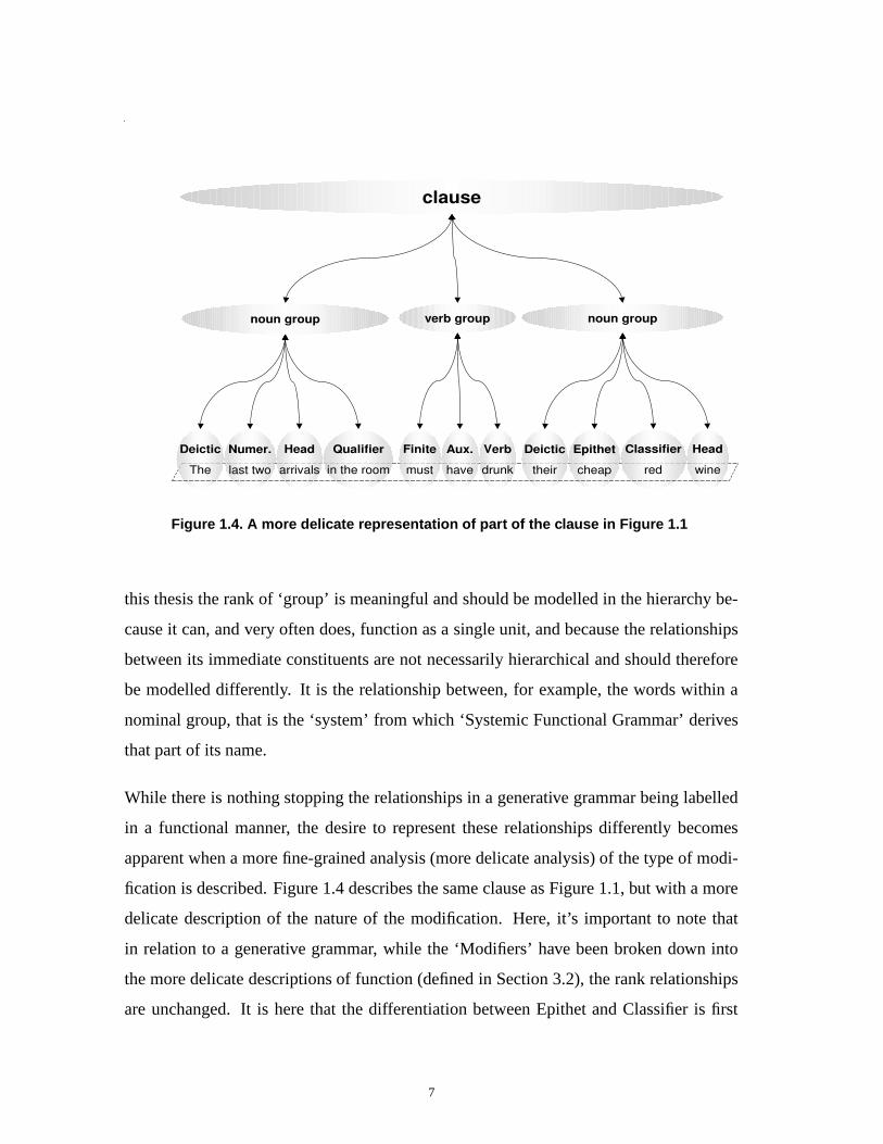
Figure 1.4. A more delicate representation of part of the clause in Figure 1.1
this thesis the rank of ‘group’ is meaningful and should be modelled in the hierarchy be-
cause it can, and very often does, function as a single unit, and because the relationships
between its immediate constituents are not necessarily hierarchical and should therefore
be modelled differently. It is the relationship between, for example, the words within a
nominal group, that is the ‘system’ from which ‘Systemic Functional Grammar’ derives
that part of its name.
While there is nothing stopping the relationships in a generative grammar being labelled
in a functional manner, the desire to represent these relationships differently becomes
apparent when a more fine-grained analysis (more delicate analysis) of the type of modi-
fication is described. Figure 1.4 describes the same clause as Figure 1.1, but with a more
delicate description of the nature of the modification. Here, it’s important to note that
in relation to a generative grammar, while the ‘Modifiers’ have been broken down into
the more delicate descriptions of function (defined in Section 3.2), the rank relationships
are unchanged. It is here that the differentiation between Epithet and Classifier is first
7

Figure 1.5. A more delicate representation of the clause in Figure 1.4
described, that is, ‘red wine’ as a type of wine, verses ‘red table’ as a quality of the table.
This is a differentiation not made by the generative grammar, describing both as adjec-
tives2 within the noun phrase. Similarly, a generative grammar doesn’t differentiate the
‘running shoe’ from the ‘running water’ or a ‘mobile phone’ from a ‘mobile society’, nor
does it claim to. It is because the function of these words is very context dependent, as
well as being more a product of the culture than the syntax, that the inference of function
is a much more complicated task than part-of-speech tagging or syntactic parsing. What is
also evident here is that the grammatical and lexical systems are not independent, in fact
in (Tucker, 1998) the opening paragraph concludes, ‘both positions suggest a integrated
approach, one in which there is no rigid compartmentalization of grammar and lexis’,
which is why the term ‘lexicogrammar’ is often given to a Functional Grammar.
Figure 1.5 gives an even more delicate description of the same clause (one way in which
it could have been further expanded is to display the rankshift in the first nominal group’s
2part-of-speech is also described within SFG, but omitted from these Figures for simplicity.
8

Qualifier, that is, the embedded Prepositional Phrase). Here, amongst other things, a
distinction is made between the types of Numeratives ‘last’ and ‘two’ into Ordinatives and
Quantitatives respectively. The delicacy of Ordinatives can be further divided into Exact
(second, third, fourth, fifth, several) and Inexact (next, subsequent, middle, previous)
Ordinatives. Some, such as ‘first’ and ‘last’ will function as either in different contexts,
while all may differ through submodification (‘almost ten’).
What such a delicate description of Numeratives gives us is why the phrase ‘the previous
three people’ is acceptable, but the phrase ‘the fifth three people’ is not.3 A person would
likely describe this as unacceptable semantically, rather than syntactically, illustrating
that both syntax and semantics may be described by a grammar, and that the mutually
exclusive relationship that prevents a Quantitative following an exact Ordinative is real-
ized paradigmatically not syntagmatically, that is, it is a product of the larger system of
language and not a simply a constraint between types of Numeratives. This demonstrates
that, given a sufficient level of delicacy, a grammar will have the ability to distinguish the
semantically acceptable from the semantically nonsensical.
Another illustration of how semantics may be realized in a grammar is in the well used
sentence ‘colorless green ideas sleep furiously’. This was invented by Chomsky who used
it to conclude that, ‘such examples suggest that any search for a semantically based defi-
nition of "grammaticalness" will be futile’ (Chomsky, 1957). While this seems to be true
in a generative grammar, it is not the case in a functional grammar. It is easy to imagine
a level of delicacy at which selectional restrictions constrain the possible ways in which
terms including ‘ideas’ may be modified. It is at this point of failure that the grammar
describes why this sentence is nonsensical. A similar, but deterministic, model for se-
mantics within a generative grammar was given in (Chomsky, 1965), but this inclusion
of semantics was not extended to probabilistic realisations within the generative school.
3it was pointed out to me that the phrase ‘the fifth two animals on the ark’ is acceptable, but this is realizedslightly differently as ‘fifth’ doesn’t operate as selectional restriction on ‘two’, but as an ordering restrictionon ‘two animals’ and would do so even if ‘animals’ was absent through ellipses. However, it stands asa good example of the close relationship between grammar, lexis and context, and that the relationship isrealized paradigmatically, not by a property belonging only to a single word.
9

More recently, the minimalist program has made some small concessions to semantics to
prevent over-generation in X-Bar theory. It’s important to note that while many of the
schools of linguistics that have come out of the generative school (including those dis-
cussed below) do give an account of semantic and/or lexical constraints, they are usually
described as constraints on the syntax, not an inherent part of the grammar.
This model of SFG, where increasing levels of delicacy leads to greater selectional con-
straints about what and how items may be used, has given rise to two important concepts:
lexis as most delicate grammar, and language as choice. These neatly complement each
other.
Lexis as most delicate grammar (Halliday, 2002; Halliday, 1978; Hasan, 1987), describes
how, at the (theoretical) finest level of delicacy, the number of constraints has increased to
where only one word (lexeme) could possibly fit that slot, and more importantly, as each
level of delicacy refined, the selectional restrictions are more constraining. Although there
are similarities between these and the selectional restrictions imposed by the early forms
of generative grammar and the subcatagorization frames of Head-driven Phrase Structure
Grammar (HPSG), there are a few fundamental differences. Firstly, the restrictions be-
long to a point of delicacy of the grammar, and not to specific words, secondly, there is no
implicit directionality in the constraints, and finally, the constraints are only probabilistic
and if broken the grammar does not break down or lead to ‘linguistic malias’ (Hasan,
1987; Tucker, 1998). Why it is probabilistic is that ‘colorless green ideas sleep furiously’
is perfectly acceptable given the right context. John Hollander conspicuously uses it in
Coiled Alizarine, but only in that it is recognising the nonsensicality. That is, the poem
is aware that there is a point of delicacy at which the sentence becomes semantically un-
grammatical, which describes (perhaps a little dryly) why ‘the description of a language,
and the analysis of texts in the language, are not - or at least should not be - two distinct
and unrelated operations’ (Halliday, 1985).
Language as choice (Halliday and Matthiessen, 1999) describes how at each level of
delicacy a choice is made within the system about how to formulate the speech act. In
10

describing a given language, dialect or register, the level of delicacy needed to describe
its function will vary, both due to the nature of the language/discourse being studied and
the goals of the study itself. One thing that should remain constant is that all labels given
should not be thought of as labels applied to categories, but to meaningful tendencies
within a largely continuous system. This is not merely the ‘raw’ apriori probability given
by the observed relative frequencies of the realizations of parts of the system, but as
a system of truly indeterminate boundaries, allowing for multiple parts of the system
to overlap and be concurrently realized. It is the relative emergence of these various
phenomena in different systems that allows studies to be undertaking comparing different
languages, registers, contexts or content, or as is often the case in NLP, to classify based
on them.
Within SFL, meaning is often described as function plus context/discourse. The latter are
best described in (Thompson, 1999; Knott et al., 2001).
While syntactic structure should inform computational tasks that are largely semantic,
mapping a generative grammar to semantics is problematic, as by definition, a gener-
ative grammar excludes semantics. Nonetheless, HPSG (Pollard and Sag, 1994) does
describe how roles relating to the metafunctions at the level of clause will map to a gen-
erative structure, which has been demonstrated in computational work (a more thorough
description of the relationship between SFG and HPSG is given in (Bateman and Teich,
1991)). Similarly, Lexical-Functional Grammar (LFG) (Bresnan, 2001) while still being
more formal than functional, significantly extends a generative grammar to semantics and
some aspects of functionalism.4 It is by necessity that practitioners of Natural Language
Processing (NLP) working within the generative framework must include non-syntactic
features of a grammar with varying degrees of ad-hoc-ness, although often with consid-
erable success (Goodman, 2000; Collins, 1999).
4To say that LFG merely extends a generative grammar is probably like stating that SFG merely givesstructure to the linguistics of Firth, but providing a detailed description of LFG is outside the scope of thisthesis
11

The concept of ‘probability’ in grammar may be approached and defined in many different
ways, and it is explored in more detail in section 2.3. Within functional grammar, a
variation known as the ‘Cardiff grammar’ (Fawcett, 2000) has been used frequently in
computational tasks, but it doesn’t lend itself as naturally to the ‘fuzzy set’ probability
used here as it sits further down the scale towards determinism/formalism.
Another model of language that was seriously considered was that of Optimality Theory
(Prince and Smolensky, 1993; McCarthy and Prince, 1995), as it has been demonstrated
to perform robustly in terms of its ability to model language in terms of a broad variety of
phenomena, and lends itself especially well to a discussion of markedness. In particular,
it provides a model that describes constraints that are violable, and is therefore in concor-
dance with the selectional constraints of delicacy in SFG. It may be possible to discuss
markedness in SFG from an OT-theoretic point of view, as has been successfully demon-
strated in LFG (Frank et al., 2001), but as OT is a relatively new and developing theory,
especially in syntax (Legendre et al., 2001) and large scale computational work (Kuhn,
2001), it was decided that it was more beneficial to perform an analysis within an existing
model rather than greatly increasing the scope (and scale) of the project by including the
development of the theory itself.
1.4.1. Applications
As SFG’s lexicogrammar encapsulates notions of function, semantics, context and lexis,
it is relevant to most areas of NLP. Within the work presented here, the following are some
broad possible areas of application:
Translation: (manual or machine): In (Salas, 2001) words that could function as
both Epithets and Classifiers was cited as a major source of error in a manual
translation from English to Spanish, so no doubt they are even more problematic
in machine translation. It is easy to imagine ‘red wine’ mistranslated as ‘vino
rojo’, rather than ‘vino tinto’ (tinted wine). The system described here could be
used to flag items with a given probability of being missclassified in this way for
12

a manual translation, or be used for improved machine translation (Bateman et
al., 1989).
Information Retrieval and Disambiguation: Working within a HPSG framework,
(Sag et al., 2002) noted that multiword constructions were problematic in NLP.
They identified problems with verb-particle constructions such as ‘look up’ and
‘fall off’, which are described within SFG as part of the verb group. Similar
problems can be described within SFG as compound things, ‘car park’, or as
part of the Classifier-Thing relationship. The identification of pre-Deictics con-
taining ‘of’ will also improve a given representation, as it will allow the correct
identification of the Head of a group.
Probabilistic Representation: Along with the advantages discussed in Section
1.4, there are several known areas where a probabilistic representation of lan-
guage is most accurate. These are known as Ambiguities, Indeterminacies and
Blends (Matthiessen, 1995). Ambiguities are ‘either/or’ categories, with mul-
tiple interpretations exclusively possible. Blends are where multiple interpreta-
tions are inclusively possible. As their name suggests, Indeterminacies are true
probabilistic representations, lying between Ambiguities and Blends.
Creation of a corpus derived model: Provided it is guided by expert-knowledge,
a corpus derived grammar is more desirable than an explicitly defined one, as
it can capture phenomena from a much larger volume of data, and may be able
to explicitly capture register specific features of the grammar. There is also the
more controversial position that grammars that are not derived from real speech
are much more likely to be biased by the assumptions of the creator(s). This was
the motivation for developing the NIGEL grammar (see Section 2.1).
Combining lexical and grammatical approaches: A computational approach is
(potentially) not limited in the number of features it can use to describe and dis-
ambiguate text. This becomes emergent when lexical phenomena, often dervied
from large volumes such as collocational tendencies, are used alongside gram-
matical structures in the disambiguation process.
13

The grammarian’s other dream: If ‘lexis as most delicate grammar’ is the gram-
marian’s dream (Hasan, 1987), then automating the discovery and application
of lexis-as-most-delicate-grammar is what a grammarian would start dreaming
about if they attempted to undertake such a project manually.
14

CHAPTER 2
Background and Foundations
This chapter describes the theoretical foundations on which this thesis is built, and de-
scribes related computational work.
2.1. Related Work
To a large extent, this thesis is exploring new territory, in that it is novel both in its ap-
plication of machine learning to inferring a functional grammar and of its probabilistic
representation of a functional grammar.
The parsing of formal structures is definitely the mainstream of grammar processing. This
is largely due to the fact that a generative grammar is a formal structure, and can be defined
in a manner similar to many compilers. As a result, the parsing of generative models, and
indeed any formal model, is a well researched field.
While information theory and related statistical methods are not new (Kullback, 1959),
their application to the learning of language is comparatively more recent than the use of
parsers, the vast majority of work and innovations occurring since the mid 1990’s. Even
now, the term ‘inferring a grammar’ is often applied quite loosely, with many studies
actually inferring much simpler hypotheses, for example, simply determining whether or
not a given sentence is grammatical, as in (Lawrence et al., 2000). Other studies have
used more informed methods for combining semantic information with formal syntactic
structures in the inference of a context-free grammar, such as (Oates et al., 2003) where
the assumption of there existing word/meaning pairs in the lexicon was formalised and
exploited in the representation of a grammar.
For NLP tasks other than inference of a grammar, purely statistics methods are well-
defined and widely successful (Manning and Schütze, 1999). For some of these tasks,
15

purely statistical methods may be used to determine phenomena that are mostly syntactic
in nature, such as clause boundaries (Carreras and Màrquez, 2001), and part-of-speech
tagging (Ratnaparkhi, 1996).
Some of the first significant uses of mixture modelling in natural language were in (Berger
et al., 1996; Iyer and Ostendorf, 1996), where methods for creating sentence level mix-
tures were used to model topic clusters. Clusters of words are well-known to follow
probabilistic distributions (Pereira et al., 1993), and in (Li and Abe, 1998) the knowledge
of word clusters was used as features alongside syntactic information.
The learner described here may be thought of as very similar to a Maximum Entropy
learner, whose relationship to natural language extends beyond the boundaries of compu-
tational history. Perhaps the broadest context this has been given is:
The concept of maximum entropy can be traced back along multiple
threads to Biblical times. Only recently, however, have computers be-
come powerful enough to permit the widescale application of this con-
cept to real world problems in statistical estimation and pattern recog-
nition. (Berger et al., 1996)
Most practitioners, however, rarely look back past Laplace (about 200 years), who ex-
plored the derivation of probabilities from incomplete information. One of his conclu-
sions, that if there is no evidence favouring any one of multiple events, then all should
considered equally likely, informs the aspect of the learning algorithm here that allows
distributions from multiple classes to wholly co-exist if there is no contrary evidence in
the feature space.
In a recent review of current methods in NLP, (Rosenfeld, 2000), Bayesian modelling is
cited as one of the most appropriate representations for language modelling. There, it
was needed to contrast probabilistic methods with ‘linguistically motivated’ methods, as
only deterministic grammars were considered. Success was also reported from models
of dependency grammars. This is consistent with the model described by SFG, as the
16

function of a word can be thought of as a dependency relationship between it and (very
often) the Head of the group, although the relationships in SFG are often a little more
complicated than the pair-wise relationships described by most dependency grammars.
In (Collins, 1999), a model informed by HPSG was created. Within a generative struc-
ture, it probabilistically represented and classified using constraints derived through sub-
categorisation frames, adjacency trends and probabilities derived from the frequencies of
realization by seen lexical items. It showed significant improvement over existing meth-
ods, both in the combination of feature types and learning method, and the accuracy of
results.
Supervised machine learning algorithms are typically restricted to classifying labels or flat
structures. The first significant extension of this to the supervised learning of structure was
in (Sperduti and Starita, 1997), where the architecture of a neural network was trained to
a given structure.
An important step in the learning of structure for natural languages is in (Lane and Hen-
derson, 2001) where a probabilistic neural network was effectively mapped to a generative
syntax. In order to maintain an�������
scalability they restricted the depth of the syntax (to
three levels), similarly bound the potential complexity of the inferred grammar, and re-
stricted the testing to sentences of less than 15 words. As they point out, this didn’t greatly
affect the performance on the corpora of news reporting, but it would not transfer well to
other registers or to spoken language without considerable concessions or additions.
An area where machine learning has been demonstrated to be a particularly useful method
is word sense disambiguation. A good review of this in relation to wider NLP is given in
(Màrquez, 2000).
In Systemic Functional Grammar, computational representations (Bateman et al., 1992a)
and applications to artificial intelligence (Bateman, 1992) are not new, but the majority
of work in this area has focussed on language generation (Matthiessen, 1983; Mann and
Mattheissen, 1985; Matthiessen and Bateman, 1991; Bateman et al., 1992b).
17

(Cross, 1993) gives the first discussion of the relationship between collocation and lexis
as most delicate grammar in the computational context.
Although machine learning has not previously been used in the inference of a Systemic
Functional Grammar, the need for functional information in NLP tasks is well known
(Matthiessen et al., 1991), and there have been two notable implementations of an at-
tempt to learn a functional grammar by context-free parsing methods that include Sys-
temic Functional information.
The first is WAGSOFT (O’Donnell, 1994). It was the first parser to implement a full
SFG formalism and performed both parsing and text generation. However, the parser was
limited in the complexity of the sentences it could analyse, and the parsing function was
removed from later versions.
The second is (Souter, 1996). It was probabilistic only in the sense of levels of confidence
- the actual grammar consisted of deterministic rules. Given the generous performance
evaluation criteria that if one of the top six most confident parse trees was the correct one,
an accuracy of 76% was obtained for a corpus of spoken English. The main shortfall
was efficiency - the parser took several hours to parse a single clause (by contrast, the
algorithm described here, Seneschal, learned the grammar from about 10,000 words in
less then a minute, and classified the raw text (test files) of about 4,000 words in a couple
of seconds), but it could possibly be made more efficient with using recent advances in
parsing technology.
Some earlier implementations of SFG parsers, but with more limited coverage, include
(Kasper, 1988), (O’Donoghue, 1991) and (Dik, 1992).
For the German language, (Bohnet et al., 2002) implemented a successful method for
the identification of Deictics, Numeratives, Epithets and Classifiers within the nominal
group. The learning method relied on the general ordering of functions and observed
frequencies. Where a word could possibly belong to two adjacent functions, the ambiguity
was resolved by assigning it to the most frequently observed function for that word. These
18

frequencies came from groups without ambiguities, and in turn, the frequencies were
updated once there was evidence to classify an ambiguous group. This bootstrapping
process1 iterated until no more functional ambiguities could be resolved. They were able
to assign a function to 95% of words, with a little under 85% precision.
There have been some recent successful uses of features derived from Systemic Func-
tional Linguistics in document classification tasks that utilised machine learning (O’Donnell,
2002; Herke-Couchman and Whitelaw, 2003). While they didn’t attempt to learn a gram-
mar, it is good evidence that the output of the system described here would be successful
for NLP tasks.
2.2. Machine Learning
This Section defines machine learning as it relates to the work described here, and dis-
cusses why the algorithm defined in Chapter 4 is an appropriate development for repre-
senting, classifying and analysing a functional grammar.
Unsupervised clustering attempts to discover an optimal representation of a data set such
that the data is divided into multiple clusters. The goal of such a task is typically the
knowledge of that classification, given by the cluster definitions in relation to the distri-
bution of items between clusters, and the distribution of attribute values between clusters.
Supervised machine learning is a branch of artificial intelligence that uses statistical meth-
ods to make informed classifications of unlabelled data. As input, a machine learning
algorithm takes a training set of items with known classifications, each with a set of cor-
responding attributes. It then infers a model about what combinations of these attribute
values result in the given classifications. This model is applied to a test set of items, as-
signing classifications to them, with the success typically gauged by the accuracy of these
classifications. The goal of supervised learning is typically the building of a classifier for
classifying unlabelled items.
1see Glossary for a formal definition
19

Semi-supervised learning is a term applied to any combination of supervised and unsu-
pervised learning, including an unsupervised classification seeded with some number of
labelled items, and using unlabelled items in creating clusters for a supervised classifica-
tion.
2.2.1. Types of machine learning algorithms
There are a number of types of machine learning algorithms that may have been used.
Decision trees (Quinlan, 1993; L. Breiman and Stone, 1984) work by recursively splitting
the data set on one attribute at a value that optimises the distribution between classes. De-
cision graphs (Oliver, 1993), extend decision trees by allowing joins as well as splits. The
leaves of the tree/graph are given the classification of the majority class of the items within
that leaf. Decision trees/graphs were not considered here as they do not naturally produce
a probabilistic classification distribution (although recent advances are addressing this
(Provost and Domingos, 2003)), and cannot be accurately used to calculate an attribute’s
contribution to a classification as a highly significant but correlated attribute may never
be split on. As the splits are made according to only one attribute, the resulting classifi-
cation is necessarily grid-like, and as such is a little unsophisticated in the description of
the class distributions across the attribute space. Nevertheless, decision trees/graphs have
been shown to produce high accuracies and have been shown to respond well to boosting
algorithms.
Support Vector Machines (SVMs), or Kernel Methods, work by dividing the attribute
space according to given mathematical function(s). For example, given a data set with
two classes A and B and two attributes x and y, a linear kernel might look for the optimal
equation: ��� ������� , in terms of how that line divides the attribute space into regions
containing optimally pure distributions of � and � . While the distance from the line may
be used as a probabilistic distribution (least squares regression is a popular metric for this),
this is more a measure of confidence than gradational probability. The biggest drawback
of SVMs is that they typically don’t support multistate attributes. An additional hurdle
20

is the very large number of possible kernels and parameters, the appropriate selection of
which is necessary for an accurate classification, which is itself a large field.
Neural networks, which model their learning process on the biological construction of
neurons, have been developed with many different architectures, with most also seeking
to divide the attribute space according to given mathematical functions, although they can
learn and define a probabilistic distribution. They also suffer from the problem of there
being a large number of possible heuristics and parameters. Further, many networks are
problematic in that, like decision trees, they cannot be accurately used to calculate an
attributes contribution to a classification.
Bayesian methods are well established, and currently enjoying a resurgence in interest
in machine learning (Lewis, 1998). A Bayesian learner is term that is applied to any
learner that (perhaps only loosely) follows the Bayes’ rule, that the probability of an item
� belonging to a class � is given by:
(1) � � ��� � � � � � � � �� ����� �� � � �
The problem with this is that it assumes that attributes are independent of each other,
which is why it is described as Naïve Bayes, the advantage being that this has� � � �
scalability and may only require one pass over the data if the attributes are multistate.
Extensions of Naïve Bayes to learners that capture attribute correlations include Lazy
Bayesian Rules (LBR) (Zheng et al., 1999), which can find a correlation between an
attribute and at most one other for approximately������� �
cost, and the recent Averaged
One-Dependence Estimators (AODE) (Webb and J. Boughton, 2002), which can find a
correlation between an attribute and at most one other, but is optimised to approximately� � �� �
cost.
Clustering is a (usually) holistic technique that seeks to group items in clusters according
to algorithms that typically take all attributes into account simultaneously, and is most
commonly used in unsupervised learning. Within a large variety of clustering approaches
(Berkhin, 2002), mixture modelling is a methodology that assumes a given data set is
21

the sum of simpler distributions. The discovery of the ‘intrinsic classification’ here is the
discovery of an optimal representation as described by given statistical methods. Unsu-
pervised mixture modelling is much more developed than supervised learning, with some
unsupervised mixture modelling algorithms originally conceived and developed in the late
1960’s (Wallace and Boulton, 1968).
Mixture models (McLachlan and Peel, 2000) typically perform better than clusters based
on apriori distance measures, such as a nearest neighbour algorithm, as they allow lo-
calised variation in the significance of ‘distance’ according to that described by the data
itself.
More recently, work has given rise to the use of hybrid algorithms. Within Bayesian
related supervised techniques, the hybrid algorithm NB-Tree (Kohavi, 1996), combining
decision trees with a Naive Bayes classifier, is one of the most successful recent develop-
ments, and one that is used in benchmarking here.
No one machine learning algorithm can be the most accurate across all possible data
sets (Wolpert, 1995), and even within a single data set, different aspects may be bet-
ter described by different learners. Automating the selection of a good classifier for a
dataset and using multiple classifiers on the one set has given rise to the areas of machine
learning known as meta-learning (Vilalta and Drissi, 2002) and ensemble learning (Di-
etterich, 1998). The development and explicit definition of a learner is desired here, so
meta-learning is not appropriate, and neither is ensemble learning as calculating attribute
significance across multiple classifiers is complicated. Nonetheless, the underlying as-
sumptions of both are present in the search to describe a single target class as the sum of
simpler subclusters, as defined in Chapter 4.
2.3. SFG as a Probabilistic Model of Language
Language is widely regarded as having probabilistic properties, but in computational work
this is usually treated as a hurdle to overcome (Bunt and Nijholt, 2000), not a phenome-
non to attempt to explicitly represent and exploit. As most grammatical investigations in
22

computational linguistics have utilised a generative grammar, probabilistic distributions
have most commonly been used as confidence measures from which a single deterministic
model is chosen.
Given the lack of probabilistic structure in a generative grammar, it is worth investigating
the roots of this. As discussed in the introduction, a generative grammar is a cognition-
driven theory that assumes the structure of language is the product of the generation of
binary rules. This stems from (Chomsky, 1957) where it was shown that a hierarchy may
be defined long distance relationships, and be expressed as a set of binary rules. While
the structure itself is not overly significant,2 what was most interesting was the theory
that language was produced by an act as simple as the generation of a hierarchy of binary
rules, which meant that the grammar itself must be deterministic.
The dismissal of probability is ‘one’s ability to produce and recognise grammatical ut-
terances is not based on notions of statistical approximation’ (Chomsky, 1957). This is
not, as has been claimed, a straw-man argument attacking Firthian linguistics that allowed
Chomsky to ignore the probabilistic nature of language, it is simply a misunderstanding
of the use of statistics, and as a statement is correct. By way of analogy, a generative
grammar’s use of a representation such as ‘S � NP VP’ should not described as being
based on notions of arrows, that is, the ‘ � ’ is simply an efficient way to represent the
underlying deterministic rule. Similarly, statistics is simply an efficient way to represent
meaningful trends in what is underlyingly a continuous system.3
2Although a deterministic hierarchical grammar may be imposed upon any contiguous set with recursiveordering tendencies, Chomsky’s syntax still stands as the simplest and most ingenuous way of expressingthe recursive nature of syntax in isolation. The momentum of the revolution it caused in American Struc-turalism can still be seen, as Linguistics is one of the last fields, in Science or the Humanities, to let go ofmany structuralist assumptions3The most convincing argument for a rule based generation of language was that it was the simplest expla-nation for the rate of language acquisition, as it was assumed that it was easier to learn/set deterministicrules than to learn as trends in a gradational system. On a slight tangent, recent work computational work(Brent and Cartwright, 1997; Dowman, 2002), has provided evidence against this. In particular (Dowman,2002) has shown that the acquisition of colour terms occurs with surprising speed in probabilistic learning.This is not to say that machines learning is equivalent to human learning, simply that as machine learnersare much less sophisticated and can’t ‘experience’ colour, but are nonetheless able to acquire the correctusage, it seems language acquisition is not a difficult task requiring dedicated, specialised structures. Thisdoesn’t prove that language acquisition isn’t the result of the setting of binary rules, it simply shows that
23

Systemic Functional Grammar is a probabilistic model of language. It has always been
described as such (Halliday, 2002), with the further qualification that it is probabilistic in
the manner of ‘fuzzy logic’. That is not to say that there are not sharply defined boundaries
within this. In phonology, for example many languages make a sharp distinction between
voiced and non-voiced, while the distinction between voiced and strongly-voiced is over-
lapping and context dependent.
It is important to note that a probabilistic distribution is not merely a measure of confi-
dence, a ‘fuzzy logic’ probability is one where the gradation and overlap is itself mean-
ingful. Nor is it necessarily determined by simple counting the frequencies of observed
phenomena (although this is one possibility). The probability is best thought of as a con-
ditional probability, that is, the probability given by a set of circumstances.
It is, of course, easier to discuss any meaningful trends in probabilistic distributions as if
they were hard categories, and much of discussion in this paper does exactly that.
what was thought to be strong evidence in favour of it has turned out not to be. In either case, the cognitiveaspects of language are outside the scope of this thesis.
24

CHAPTER 3
Definition of Functions
This chapter defines the functional categories of words that will become the targets of the
classification. These are defined and discussed in terms of their function, the phenomena
that may differentiate one function from another, and the finer layers of delicacy.
In data-mining parlance, the word functions defined here will become the targets, their
instances in the texts becoming the rows, while the definitions given here inform the
choice of features that will become the columns defined in Section 5.1.
The definitions given here are those defined in (Matthiessen, 1995) and (Halliday, 1985).
Table 3.1 gives a list and example realization of these.
3.1. Groups / Heads:
All groups have one (or possibly more) words forming the Head of the group. The other
terms in the group, the modifiers, are loosely arranged in the order of their effect on the
Head. A general ordering can be seen in that the more permanent or intrinsic the type
of modification, the closer it will be placed to the Head. The naming convention that
describes which constituent is the Head is pretty straightforward:
Verbal Group Head: the Verb (event / lexical verb)
Prepositional Group: the Preposition
Nominal Group: the final term in the group, excluding qualifiers (embedded final
position prepositional phrases or adverbial groups).
Adverbial Group: the Adverb
Conjunctional group: the Conjunction
25

Group Function (Target Category) Example Sentence
Verbal Finite couldAuxiliary haveEvent / Lexical Verb beaten
Nominal Pre-Deictic some ofDeictic thePost-Deictic famousOrdinative topNumerative tenEpithet wealthyClassifier tennisThing players
Adverbial Adverbial pre-modifier moreAdverb quickly
Prepositional Prepositional pre-modifier longPreposition before
Conjunctional Conjunctional pre-modifier onlyConjunction ifConjunctional post-modifier only
Table 3.1. Example of Group/Word Function Classifications
3.2. Definition of Word Functions
Strictly speaking, the term ‘modifier’ describes a Logical function and the other terms
given below and in Figure 3.1 are Experiential functions. For the study undertaken here,
the term ‘modifier’ is sufficiently detailed enough to describe the functions in the instances
it was used, as all these were too rare to define in terms of finer delicacies.
The following definitions are sufficient for the work here, see (Matthiessen, 1995) and
(Halliday, 1985) for a more thorough description.
3.2.1. Verb Group
Finite: The first Auxiliary in a verbal group. It’s the verbal equivalent of a Deictic,
fixing the group in relation to the speech exchange. The Finite is actually a prop-
erty of the verb group, which means that when there is only one word realizing
the verb group, it is conflated with the lexical verb. Here such realizations are
26

simply labelled as the lexical verb, as the further identification that they are also
the Finite would be simple.
Auxiliary: An intermediary Auxiliary in a verbal group. Auxiliaries may modify
the event through modality and/or probability.
Verb (Event/Lexical Verb): The head of a verbal group - the action itself. It may
be phrasal (consist of more than one word):
verb + adverb: ‘seek out’,
verb + preposition: ‘look for’,
verb + adverb + preposition, ‘look out for’.
3.2.2. Prepositional Group
Prepositional pre-modifier: Modifying a preposition
Preposition: Expresses grammatical and/or semantic relations between elements.
3.2.3. Nominal Group
Pre-Deictic: An embedded phrase or a term pre-modifying the Deictic. ’the king
of the hill’, ‘give it to all the people’. ‘one half the people’. An ‘of’ may be
required before the Deictic by some partitives, and ambiguity can appear here:
‘one of the boys’ - is ‘one’ the head, and ‘of the boys’ a Qualifier, or is ‘one of’
a pre-Deictic?
At a finer layer of delicacy, a Facet describes part-of relationships, ‘the back
of the house’, and a pre-Numerative describes Quantitative and Ordinative rela-
tionships, ‘0.05 of a second’.
It should be noted that Sinclair posits that ‘of’ can also indicate a third func-
tion, where the items before and after the ‘of’ jointly form the semantic head, as
in titles such as ‘the King of Brunei’ (Sinclair, 1991), but these have not been
modelled here.
Deictic: Deictics fix the nominal group in relation to the speech exchange. They in-
clude Demonstratives (‘this’, ‘that’, ‘those’), Articles (‘the’), indefinite Articles
(‘some’, ‘every’, ‘a, ‘all’, ‘both’, ‘enough’), and Possessives (‘my’, ‘his’, ‘their’,
27

‘Rob’s’, ‘Dr Smith’s’). When a Possessive is realized by a Genitive phrase, sub-
stantial embedding is possible (‘the man who used to live down the road but
doesn’t anymore’s car’).
Post-Deictic: An adjective that modifies the Deictic not the Thing. In (Matthiessen,
1995) these are simply called adjectives, and refer to the rare but grammatical
situation of an adjective occurring between a Deictic and later functions, for ex-
ample, ‘lucky’ in ‘the lucky first three placeholders’. In the corpora used here,
there were only two instances of a post-Deictic, both in groups without Numer-
atives, and so for testing they were labelled as Epithets.
Ordinative: An Ordering Numerative, (‘first’, ‘second’, ‘3rd’, ‘4th’, ‘last’). When
indicating a selectional restriction on a numeral it commonly occurs with a Quan-
titative (‘the first 3’, ‘the last two’).
Quantitative: A Quantitative Numerative. May be numbers, (‘one’, ‘two’, ‘3’,
‘4’), or expressions, (‘many’, ‘several’, ‘few’, ‘lots of’, ‘two’, ‘more’).
Epithet: Describing some quality or process of the Thing. At a finer layer of del-
icacy there are Attitudinal Epithets, ‘the ugly lamp’, and Experiential Epithets,
‘the big lamp’. They are most commonly realized by an adjective, but are also
commonly realized by a verb, ‘the running water’.
Classifier: Subclassification of a Thing. Classifiers are commonly realized by a
noun, ‘the table lamp’, a verb, ‘the reading lamp’, or an adjective, ‘the red wine’,
but other realizations are also possible. Classifiers are commonly though of as
providing a taxonomic function, but it may also be used to provide information
about the Head. For example, ‘table lamp’ might refer to a special type of lamp,
or simply a lamp you would expect to find on a table.
Thing: Some entity, be it physical, ‘the lamp’, or abstract, ‘the idea’, which will
most commonly be the Head of the nominal group, undergoing modification by
the other noun group constituents.
28

3.2.4. Qualifier:
A post-modifier, typically prepositional phrases head by a prepositional group, although
they may also be adverbial, nominal or verbal groups, or relative clauses.
3.2.5. Adverbial Group
Adverbial pre-modifier: Pre-Modifies or subcategorises an adverb
Adverb: Modifying or subcategorising a process.
Adverbial post-modifier: Used mostly for comparison: ‘not so regularly any more’
3.2.6. Conjunctional Group
Conjunctional pre-modifier: Pre-Modifies a conjunction. These are rare, and
didn’t occur in the corpora here, and were therefore not included in the testing.
Conjunction: Links or continues a speech act across groups/clauses
Conjunctional post-modifier: Post-Modifies a conjunction
3.2.7. Other Groups
While many theorists posit the existence of an adjectival group, this study conforms to
Halliday (Halliday, 1985), who describes such groups in English as a nominal group with
an adjective as Head, but there is nothing preventing the same system explicitly including
such a group. Matthiessen offers the explanation that within a nominal group there are two
subtypes, or degrees of delicacy, those with nominal Head and those with a non-nominal
Head (Matthiessen, 1995).
3.3. Features distinguishing functional categories:
Table 3.2 gives the most common realizations of part-of-speech in function within the
nominal group (more are probably possible). Within this, there are two broad reasons that
may make inferring a given word’s function problematic (manually or computationally):
the word is unknown or the word may occur in multiple functional categories.
29

Function: Deic Ord Quant Epith Cfier ThingPOS:Determiner YPronoun Y YAdjective Y Y Y YNumeral Y Y Y Y Y YAdverb Y Y YVerb Y Y Y YNoun Y Y Y YProp Noun Y Y Y Y
Table 3.2. Possible realizations of part-of-speech as function in the nominal group
3.3.1. Unknown words
Orthographic properties:
(1) Prepositions & Auxiliaries: closed groups. It can be assumed that all are known.
(2) Deictics. Articles and Demonstratives are closed groups and hence solved by (1).
For Possessives, the possessive marker, ‘Rob’s’, indicates that a proper noun is a
Possessive.
(3) Verbs and adjectives may be distinguished by affixes (eg div-ing) although this
will not distinguish between their functioning as verbs or as gerunds realizing
Epithets or Classifiers.
(4) Nouns may be distinguished by affix information indicating number (eg cat-s),
but this will not distinguish their function.
Syntagmatic and Grammatical Properties (assuming simple groups or complete knowl-
edge of all embedding and group complexes):
(1) Any word between two words of the same category must also belong to that
category. For example, in ‘the big shmock ugly table’, ‘shmock’ must function
as an Epithet.
(2) In the verbal group, the final word is always the lexical verb.
(3) In the verbal group consisting of more than word, the first word is the Finite, and
any intermediary ones are Auxiliaries.
30

(4) All sequences are loosely bound by the order in which they are defined Sec-
tion 3.2. (Although in practice, embedding and complexes will allow almost
any sequence of functional classifications, albeit with differing constraints and
probabilities).
(5) If two words are linked through conjunction, ‘the electric or mechanic type-
writer’, then they will often have the same function.
(6) Given a grammar and all possible parses, only one functional category may be
possible in a given context. It can be assumed that all sequential constraints are
a subset of grammatical constraints.
3.3.2. Words occurring in multiple categories
The syntagmatic and grammatical distinguishing factors for unknown words can also be
used to disambiguate a words category:
(1) Epithets may be intensified, ‘the very red table’, whilst classifiers generally can-
not *‘the very red wine’. Some cases of intensification of a Classifier are pos-
sible ‘a very postmodern discourse’ (Matthiessen, 1995), but are rare and didn’t
occur in the corpora used here.
(2) A Classifier may elsewhere be used metonymically, for example, ‘the red wine’
and ‘the wine was a red’ *‘the table was a red’. It is important to note the Deictic,
‘a’, and that ‘red’ was the Head, indicating that this is not Epithetic, for example,
‘the table was red’ or ‘the table was a red one’. In fact, the observance of this
Epithetic use elsewhere is a good indication of an Epithet.
(3) Assuming one function per discourse, there may be examples elsewhere that are
resolved through syntagmatic disambiguation. For example, the presence else-
where of ‘a Murry river red wine’ will indicate that ‘red’ is a likely a Classifier
in ‘the tasty red wine’.
(4) Observed instances with lexico-semantic relations. For example, if ‘running’ in
‘running shoe’ is known to be a Classifier, than it is likely that the co-hyponyms
‘hiking’, ‘jogging’, ‘walking’ and are also classifiers for ‘shoe’. Similarly if
31

‘leaking’ in ‘leaking tap’ is known to be an Epithet, than it is likely that ‘drip-
ping’ and ‘flowing’ are also Epithets for ‘tap’.
(5) In some cases Classifiers may be compounded to the Thing ‘headlight’, although
this is also strong evidence that the term represents a compound Thing and not
a Classifier-Thing relationship, which is therefore closer to the phenomenon de-
scribed in (Sag et al., 2002).
(6) Where the head is a person, the potential for Classification increases, as for
humans the need to subcategorise is ‘socio-culturally more significant in the way
we categorize experience’ (Tucker, 1998).
(7) Where phonological information is available, there are often noticeable intona-
tional differences between Epithets and Classifiers. While this cannot be taken
advantage of here, it is interesting that disambiguation through local knowledge
may be possible. It also gives evidence towards the very existence of such cate-
gories.
(8) As some participles require ‘of’ before the Deictic, there can be some ambiguity
as to whether a clause contains a pre-Deictic or a prepositional phrase. For ex-
ample in ‘she was one of the people’, ‘one of’ is a pre-Deictic and ‘people’ the
Head, whilst in ‘she was queen of the people’, ‘queen’ is the Head, with ‘of the
people’ as a prepositional phrase filling the role of qualifier.
(9) Common collocations. In the example above ‘one of the ...’ may be recognised
as a common collocation and is therefore evidence of a pre-Deictic. This can
also separate a proper noun Classifier from the following Things, as in ‘Atlanta
Olympic Games’.
(10) Epithet modifying restrictions. For example, in ‘a tasty bottle of wine’, tasty
modifies ‘wine’ not ‘bottle’, and so ‘a tasty bottle of’ acts a pre-Deictic, even
though no Deictic is present (although it could have been: ‘a tasty bottle of my
red wine’). Here the knowledge that wine, not bottles may have tasty as an
Epithet disambiguates this.
(11) Measurement terms. Almost all cases of a Pre-Deictics involve some form of
measurement (‘bottle of’, ‘all of’, ‘some of’, ‘a few of’, ‘part of’, ‘one of’),
32
which, to a large extent, are a finite set, the exception being terms for collections
of animals, ‘a siege of herons’, ‘a cache of echidnas’, ‘an unkindness of ravens’
etc.
(12) A Pre-Deictic may be used as a way of quantifying unquantifiable nouns: ‘a
large cup of tea’.
3.4. Self-Imposed Restrictions
Deliberate restrictions were imposed here on the types of attributes that could be used
to add an important aspects to this analysis. The attributes that are defined in Section
5.1 represent the interaction of grammatical and lexical relationships (systems), and only
these systems.
There is no recourse to knowledge bases of semantic ontologies or remembered word
lists. This means that, in effect, it is learning the lexicogrammar itself. Unlike previous
computational implementations in SFG, there are no user-defined rules for inferring the
grammar, which makes this the first attempt to computationally learn a functional lexi-
cogrammar.
Therefore, provided analysis, not accuracy, is the main goal, it is more sensible to limit
the possible features by the phenomena they represent, so as to more straightforwardly
analyse the contributions of the remaining features. On this note the following two types
of features where not included:
The words themselves: Put simply, at no point is the learner able to discover that
certain words, alone or in context, are more likely to belong to a particular func-
tional category. For example, if the training set contains ‘red wine’, the learner
can not remember that ‘red’ is a Classifier in this context, it must learn the gram-
matical and lexical properties of this structure (the lexicogrammatical system),
and then recognise these properties if ‘red wine’ then occurs in a test set. A
minor reason for this is that simply remembering words is a little trivial and
uninteresting. A major reason is that here, this would over advantage the two
33

newswire test sets. There is also evidence that a word will differ significantly in
function between registers, especially at finer levels of delicacy (Martinez and
Agirre, 2000).
There are two exceptions to this. The part of speech tagger explicitly marks
the infinitive ‘to’, and the preposition part of speech markup has been altered
to identify ‘of’ to facilitate it’s identification in Pre-Deictic/Preposition disam-
biguation.
Semantic ontologies: Another gain in accuracy could have been obtained through
the use of the WordNet semantic lexicon (Miller et al., 1990), for providing ev-
idence for the function of unknown words based on the unambiguous function
of known co-hyponyms, as described in Section 3.3.2 or any of the other se-
mantic relationships it stores. Most of the reasons for not choosing the words
themselves also apply here. There is the further limitation that the words must
actually be contained in the ontology, disadvantaging infrequent words, although
there have been several studies that describe how such ontologies may be aug-
mented computationally (Hearst, 1998; Moldovan and Girju, 2001). While many
of the functions will be determined semantically, with strong recourse to the ‘real
world’ and therefore not able to be computationally disambiguated through local
grammatical knowledge, the population of the ‘real world’ use these forms and
therefore many of these functions will be emergent over large scale variation in
unlabelled text. In addition it makes the system more language independent, as
the existence of large semantic ontologies is mostly limited to a small number of
European Languages.
34

CHAPTER 4
Seneschal: A supervised mixture modeller
4.1. Introductory remarks
Here a supervised mixture modelling machine learning algorithm, Seneschal, is proposed
that learns and represents the data as probabilistic distributions. Clusters representing
different classes may overlap partially or even completely co-exist if the feature space
describes them as having identical distributions.
As was discussed in the introduction, the level of delicacy that is desirable to represent
will vary depending on the register and nature of the investigation, and so the learner is
able to discover and represent finer layers of classification if they are emergent in the
training data.
These make this study much more robust, and less reliant on the user to explicitly define
the nature of the grammar, as delicacies defined but not captured in the feature space
will not be overfit, and delicacies not defined but captured in the feature space will be
discovered. As these probabilities are learned, not explicitly defined (itself a complicated
task (Jang et al., 1997)), the features may also be represented as multistate attributes.
Some continuous aspect of language, such as part-of-speech, are rarely represented as
anything other than multistate, and exclusively represented as such by current taggers.
A version of this chapter, with extended discussion but without explicit reference to the
rest of the work here appeared as (Munro, 2003b). Only the discussion in Section 4.5 and
the comparison with AODE differ significantly.
35

4.2. Information measures
There are many different heuristics that may be used in mixture models, such as the EM
algorithm, Bayesian measures, Minimum Description Length (MDL) and Minimum Mes-
sage Length (MML). These techniques all seek an optimal model for a data set by utilis-
ing an entropy or information measure (IM). The measures used here roughly correlate to
those of MML, but as they differ and also relate to the other measures the more generic
term IM is used throughout.
4.2.1. Multistate attributes
These are also known as discrete, multinomial and/or categorical attributes.
Given an item�
with value���
for multistate attribute � , and given that���
occurs in cluster
� with frequency � � ����� � � , within the data set � ,�’s information measure for � multistate
attributes for � with size � � � � is given by:
(2) � � ��� � � � � ��������� � �� ����� � � ���� � � � �
Where
is given by the constant:
(3) ��� � � � ����� � �
� � ����� � � � � � � �
Here, it is assumed that the relative probability of attribute values are the apriori relative
frequencies of the entire set given by
.
4.2.2. Continuous attributes
In the current implementation, all continuous attributes are treated as Gaussian, assuming
a normal distribution. Put simply, the IM of an item�
in a cluster � , for a given attribute�
correlates to the�’s value for
�in relation to the mean and standard deviation of
�in � .
36

Given an item�
with value���
for continuous attribute�
,�’s information measure for �
continuous attributes for a cluster � that for attribute�
that has an average of ��� � and
standard deviation of ��� � is given by:
(4) � � ��� � � � �� ���
� ��� � ��� � � � �� � �
4.2.3. Cost of cluster membership
Many clustering algorithms employ some additional penalty correlating to the number
and/or size of clusters. Here, the cost of cluster membership has been replaced by the
inclusion of a simple prevalence threshold, indicating the minimum size a cluster may be
without being considered noise, as it was not desirable that the classifier be sensitive to
the relative frequencies of realisation in training set, as this will differ significantly across
the different registers being tested.
4.3. Algorithm Description
The steps here are: building the classifier; classifying test items and classification analysis.
4.3.1. Building the classifier
After a rough initial division into subclusters, the algorithm iteratively attempts to reduce
the overall IM by reassigning single items between subclusters, and combining or splitting
whole subclusters. Like the EM algorithm, these actions are only taken when they result
in an improved IM. The model is considered built once no improvements are possible.
This proceeds as follows:
Initialise: the data space is initially split into a multidimensional ‘grid’, with di-
visions existing at the average value of each continuous attributes, and at plus
and minus one standard deviation. For multistate items, they are simply divided
37

according to attribute value. Items are initially assigned to a subcluster corre-
sponding to the grid described by that item’s attribute values. This gives a very
rough division of the data into subclusters, its advantage being that, once the av-
erages and standard deviations are known, it only requires a single pass over the
data.
Reassign: for each item, calculate if it possesses a lower IM for a subcluster other
than the one it is currently a member of. If so, reassign the item to the subcluster
for which it has the lowest IM.
Combine: for each pair of subclusters, combine them if it results in a lower overall
IM for the items in both clusters.
Split: when an item is assigned to a subcluster (or reassigned to the same subclus-
ter), it is also assigned to one of two child clusters of that subcluster. The choice
of which to assign it to is also based on the IM of assigning the item to each
child cluster. If the overall IM of the two child clusters is less than that of the
subcluster, then the subcluster is split into two subclusters corresponding to the
two child clusters. While the method here does not guarantee an optimal distri-
bution between child clusters, it can be seen as a good approach to the extent that
using an IM is better than a random distribution, and it will also scale better than
iteratively attempting random redistributions.
In all the above steps, a constraint maintained throughout is that no training items are
allowed in a cluster containing items of another class.
Many semi-supervised models build unsupervised models over the entire data set, and
then assign a class to each cluster according to the most frequent class of the items in that
cluster. This has not been implemented here, as once these clusters have been assigned
a class it must be assumed that all items in that cluster known to not belong to that class
are either noise or misclassifications. If this is the case, than those items should not
have contributed to defining or creating that cluster. In effect, it is training to noise, and
therefore prone to overfitting. For a further discussion of the problems inherent in a semi-
supervised approach to mixture modelling see (Cozman et al., 2003).
38

4.3.2. Classifying the test items
Although this algorithm will allow semi-supervised and seeded classifications, all testing
described in this paper is for a supervised classification.
Here, after the classifier has been built, each test item is assigned the class of the subcluster
for which is has the lowest IM. ‘Ties’ were treated as an incorrect classification.
4.3.3. Classification analysis
Part of the robustness of this algorithm derives from the fact it uses the same metrics for
clustering, classification and analysis. The most obvious analysis to perform is to explore
the item membership and frequency of the subclusters of each class, but investigating the
relationships between subclusters and an attribute analysis may also be desirable.
The closeness of a cluster � � to a second cluster � � is given by the average IM of assigning
the items of � � to � � .
This value will not necessarily be the same in reverse. If � � is a relatively tight cluster,
perhaps even embedded within the range of � � for all attributes, then the average cost
of assigning the items from � � to � � will be larger, as the average number of standard
deviations from an item in � � to � � will itself be greater. If � � and � � are subclusters of
different classes, then this measure will be the amount by which the clusters define the
class membership of their items, with respect to the portion of the data space described
by these clusters.
Rather than investigating the entire IM of a cluster, comparing the IM of one attribute to
others can show which of the attributes is most significantly distributed within that cluster.
An alternative that is probably more appropriate for supervised learning is to compare the
relationships between subclusters based on one only attribute, or on a subset of them.
Significance at the subcluster level of the data is much richer than that at level of the
full set. For example, given a two-class ‘chess-board’ of items, there is no difference
39

Figure 4.1. An example of a mixture model of two classes with five subclusters in twodimensions
in the distribution of the two classes across the full set, that is, both the black squares
and white squares are uniformly distributed across both axes. Between adjacent squares,
however, the localised significance is absolute. A less severe example of this can be
seen in Figure 4.1. For���������
, the distribution along the � axis is not significant in
terms of the classification, but is of greater and varying degrees of significance for all�������
. With this information, it is easy to see how such a model may be used as tool for
feature selection. The global significance of a feature may be calculated as the weighted
aggregate of its subcluster significances, or simply the maximum of its local significances.
Figure 4.1 also provides a good example of how the effective boundary of a cluster in a
mixture model will differ from that defined by a clustering algorithm employing an apriori
distance measure. At� ��� � � ��� � �
an effective boundary exists between a relatively dense
cluster and three relatively sparse clusters. This boundary ‘hugs’ the boundary of the
40

Data set Max SVM Naive Bayes AODE NB-Tree SeneschalAdult 0.85 0.84 0.83 0.86 0.83LED24 0.67 0.73 (0.74) 0.73 0.74Mushrooms 1.00 1.00 (1.00) 1.00 1.00Tic-tac-toe 0.95 0.71 0.74 0.70 1.00Letter (0.89) 0.73 0.87 0.88 0.84
Table 4.2. Benchmark accuracy comparisons
dense cluster as, despite the large number of items, the standard deviations are relatively
lower.
4.4. Benchmarking
As this is a new machine learning algorithm, it is necessary to demonstrate its performance
against existing algorithms. In this section testing seeks to compare the accuracy of this
algorithm to other supervised machine learning algorithms, its use in parameter selection
and its use as an analytical tool.
In many ways, an accurate representation of the data is more important than an accurate
automated classification, as it is precisely the representation of the language that con-
stitutes a lexicogrammar, with the accuracy of a classification being just one metric for
determining the correctness of the inferred grammar, but it is necessary to demonstrate
that it performs as accurately as current state-of-the-art machine learning algorithms.
Here, a ten-fold cross-validation was performed on the Adult, Mushrooms, Tic-tac-toe,
and Letter data sets. The results discussed and reported in Tables 4.2 and 4.3 are from
just one of these (arbitrarily the first), as an analysis of attribute significance across mul-
tiple classifiers is itself a complicated task not undertaken here. The other nine results
showed no change in accuracy for the Tic-tac-toe or Mushrooms sets, a marginal increase
in the average result for Adult, and a marginal decrease in the average result for Let-
ter. The LED24 set, a synthetically generated set, was generated using separate seeds for
the training and test sets so that the two distributions were identically distributed but not
simply identical.
41

Although the other results in Table 4.2 were most likely obtained from different splits of
the data to those used here, it is reasonable to assume that they would not differ too signif-
icantly. The alternative of implementing all these algorithms for the sake of comparison,
is outside the scope of this research, but it’s still more desirable to present comparisons
with some of the highest reported results at the expense of precision in comparison. The
SVM result in brackets indicates that the set was reduced to a two class problem. For the
AODE results in brackets, these sets weren’t tested, so the results are estimations. The
data sets, taken from the UCI Machine Learning Repository (Merz and Murphy, 1996),
were primarily selected because many results existed for the other algorithms against
which Seneschal may be compared. Within these possible selections, the sets here were
chosen because they are among the larger UCI sets, and for the following reasons:
Adult: a variety of distributions of multistate and continuous attributes.
LED24: 7 ‘meaningful’ attributes containing 10% noise, 17 attributes are pure
noise.
Mushrooms: contains missing values.
Tic-tac-toe: a data set that many supervised clustering algorithms perform very
poorly on.
Letter: one of the larger sets, containing highly normalised variables.
The results for NB-Tree and Naive Bayes are those reported in (Kohavi, 1996) and the
results for AODE are those reported in (Webb and J. Boughton, 2002).
Although Support Vector Machines represent a large part of recent developments in ma-
chine learning algorithms, state-of-the art SVM’s often perform much better on two class
problems and typically don’t explicitly support multistate attributes. The SVM results in
Table 4.2 are, to the authors best knowledge, the highest reported results from SVM’s on
these data sets, but the search was not exhaustive.
The SVM results for the Adult, Tic-tac-toe and Letter sets are the maximum reported
values from a comparison of a number of SVM’s in (Mangasarian and Musicant, 2001).
There, multistate attributes were translated into multiple ‘binary’ continuous attributes.
42

Data set Test acc. Training acc. IGR num classes num subclustersAdult 0.83 0.83 0.5539 2 8LED24 0.74 0.74 0.0009 10 10Mushrooms 1.00 1.00 0.0007 2 81Tic-tac-toe 1.00 1.00 0.0031 2 23Letter 0.84 0.87 0.0013 26 246
Table 4.3. Benchmark classification details
For the Letter data set they reduced the set to the two classes representing the letters ‘A’
and ‘B’. When classifying only these two classes Seneschal obtained 100% accuracy.
The LED24 SVM results are from (Bhattacharyya et al., 2001) (they report an accuracy
of 73% once feature selection has removed the 17 pure noise attributes). The Mushrooms
SVM results are reported in (Rüeping, 2002).
For the Tic-tac-toe set, one of the few other supervised mixture modelling algorithms,
MultiClass, reports 98% accuracy (Roy, 1995), but learned with considerable expense
(see Section 4.5.2). With the supervised clustering algorithm COP-KMEANS, (Wagstaff
et al., 2001) reports 83% accuracy on the Mushrooms data set, but only 55% on the Tic-
tac-toe test set. See Section 4.5.3 for a discussion of this.
4.5. Discussion of this model
4.5.1. A hierarchical Representation
The extension to a hierarchical model would be fairly simple, as such representations are
common in clustering. It would be interesting to see if some features could be intro-
duced only at certain levels of such a hierarchy. Even simpler would be the use of this
model within one unit in the rank scale, assuming the hierarchical relationships have been
addressed by other means, as has been assumed in the testing here.
4.5.2. Scalability
Scalability is one of this algorithm’s strongest features, especially when it is compared to
similar learners.
43

Assuming a consistent data set, this algorithm scales linearly with respect to items, classes
and attributes. As the method treats the attributes agglomeratively and the classes inde-
pendently the linearity for these is self-evident. For items, the number of operations will
depend on the percent of items near the cluster boundaries and the number of clusters.
If the data set is consistent, the number of operations resulting from these will remain
a constant percent of the total items, and therefore also scale linearly. Testing revealed
this scalability to be slightly sub-linear, due to some operations being independent of
size, such as calculating whether or not to split or join clusters when the distributions are
known, and the transfer of items resulting from these.
By contrast, Multiclass seems to scale either polynomially or super-polynomially, al-
though a cost analysis is not given in (Roy, 1995). In terms of raw processing the su-
pervised mixture modeller Multiclass would take about an hour to process the Tic-tac-toe
set on a current PC. Seneschal takes about 10 seconds. It is for this reason, and the fact
the existence of Multiclass wasn’t discovered until after Seneschal’s development, that the
relationship between the two has not been fully explored. Of the other learners described
here, only Naive Bayes also scales linearly.
4.5.3. Attribute Correlation
In (Munro, 2003b) it was stated that Seneschal discovered local significance but not at-
tribute correlations. This is true only for continuous attributes, in that it assumes the axes
of a cluster are parallel to the space defined by the continuous attributes. It should be
clarified that for multistate attributes, local significance is attribute correlation.
Subclusters for multistate attributes seek to create clusters whose attributes are as ho-
mogenous as possible. Therefore, clusters will be formed that explicitly capture as many
correlations between attributes as possible. In effect, it is a linearly scalable solution to
the Bayes attribute independence assumption.
Where capturing attribute correlation might lower the accuracy is where the attribute cor-
relations are not significant with respect to the classification, which may be the cause of
44

the large number of subclusters and overfitting that reduced the classification accuracy of
the Letter data set.
The Tic-tac-toe data set provides a good model for analysis as the relative significance of
the attributes, each representing a square on the board, should be well-known to anyone
who’s played the game. As expected, the ‘middle square’ attribute was reported as most
significant, given by the lowest aggregate IM over all subclusters. Interestingly, within
single subclusters, it was reported as either very significant or not significant. Intuitively,
it is likely that this is due to the fact that the middle square is irrelevant if a winning
row exists along one edge. The ability of Seneschal to correctly learn this hypothesis
demonstrates its ability to capture attribute significance. It the inability to do this that
(Wagstaff et al., 2001) cite as the cause for COP-KMEANS’ poor performance. As the
correlations are across more than two attributes, and for one attribute with more than one
other, it was also a hypothesis more complicated than AODE attempts to fully capture.
45

CHAPTER 5
Experimental Setup
5.1. Corpora
One training corpus and four test corpora are used. The process of manually tagging the
corpora with the correct functions took about 20 hours. It required a large volume of input
from other people. Including validation by another linguist, it required consultation with
people familiar with the sports/disciplines discussed in the texts, as even a linguist might
not be able to identify all functions without domain knowledge.
The corpora contained many instances of what might be considered ‘noise’, in the form
of header information, dates, incorrect spellings, ‘ungrammatical’ sentences and sections
that are simply tables of numbers. After some consideration, it was decided that these
should not be removed and remain uncorrected. A robust learner should be able to recog-
nise and/or parse errors and changes in form, and the treatment of such cases by the
learner may well be interesting in itself. The only major change made to the corpora was
the representation of punctuation as attributes of the adjacent words.
Extracts from all the corpora are given in Appendix G.
5.1.1. Training corpus
The training corpus is 10,000 marked up words from Reuters sports newswires from 1996
The choice of Reuters was based on the fact that it is one of the most common sources of
text used in Computational Linguistics and Natural Language Processing. The choice of
only sports newswires was for two reasons:
(1) Taking the corpus from only one register was desirable for testing purposes (it
is arguable that Reuters political, financial and agricultural reports are separate
registers).
46

(2) Sports terminology is well known to be quite idiosyncratic and therefore both a
well distinguished register and a difficult/interesting one to look at. It is neces-
sary to learn that in cricket, a ‘one-day match’ is a type of match, a ‘1,000 metre
race’ is a type of race, and ‘2nd place’ is a type of place.1
5.1.2. Testing corpora
Four testing corpora were used, all of approximately 1,000 words. The register (domain)
dependence of NLP tasks is well known (Escudero et al., 2000), and they were drawn
from a variety of registers:
(1) Reuters sports newswires from 1996. The same corpus as the training set.
(2) Reuters sports news from 2003. This is presumed to be the same register, but is
included to test the extent to which ‘topic shift’ is overcome.
(3) Bio-Informatics abstracts. These will test the domain dependence of results in a
register with a high frequency of rare words/phrases, and with some very large
and marked Classifier constructions.
(4) An excerpt from a modernist fiction. ‘The Voyage Out’, Virginia Wolf (1915).
This was to test the domain dependence of results in a register that is more Epi-
thet frequent, and has more complicated modifications within the verb group.
These four test corpora are abbreviated as Reuters-A, Reuters-B, BIO-INF and MOD-FIC
respectively.
5.2. Attributes
Each item/instance in the data set represents instance of a one word. The attributes used
are divided between those representing grammatical features, and those representing lex-
ical features. A representation of these with an example sentence is given in Figure 5.1.
1The markup for Ordinatives functioning as marked Classifiers follows the argument that anything on thepodium is a Classifier, and everything else (except possibly last place) is an Ordinative, although there werealso uses of ‘1st’, ‘2nd’ and ‘3rd’ in the corpora that functioned simply as an ordering, which were correctlylabelled as Ordinatives.
47

Figure 5.1. An example sentence with descriptions of the attribute space
5.2.1. Grammatical
The grammatical features used here are those corresponding to the levels below and above
word function: group types and part-of-speech.
The one manually encoded feature here are the groups, as this thesis is most interested in
looking at function within the group. The automatic identification of groups and group
boundaries would require a different feature set than those described here, but would be
a fairly simple task. A brief test showed that even with the feature set described here
(minus the group-related attributes), the identification of groups occurred with around
95% accuracy.
The part-of-speech tagger used was mxpost (Ratnaparkhi, 1996), as it uses a learning
method similar to the one describe here to assign parts-of-speech, and is one of the
48

most accurate POS taggers currently implemented. It was augmented slightly, as it over-
zealously assigning the parts-of-speech of proper noun to capitalised words, due to it
being trained on corpora whose capitalisation occurs more often in this way. A similar
problem exists in that it under identified numbers, especially when represented as words,
not numerals. A set of attributes was introduce to augment this. An attribute indicating
whether a word was initial or fully capitalised was included, as were attributes indicating
whether or an Ordinative or Quantitative type number was present. The Ordinative was
simply an indication of whether the word was suffixed with a ‘-st’, ‘-nd’, ‘-rd’ or ‘-th’,
which will over-assign, but will do so for both the training and test sets in a predicable,
and learnable, way.
5.2.2. Lexical
Lexical attributes describe the collocational tendencies of terms and their self-collocation
with respect to document boundaries.
The collocations were obtained using the alltheweb search engine, as it reports the number
of web documents containing a searched term, and could therefore be used to automati-
cally and efficiently obtain collocations from an extremely large source of examples. For
two terms ‘A’ and ‘B’, the collocational tendency of the two is defined as the percentage
of number of documents containing both ‘A’ and ‘B’, divided by the number of documents
containing the bi-gram ‘A B’. Given that a word has two collocational attributes, with the
previous and next terms, an attribute was also included that describes the ratio between
the two, as explicitly capturing a ratio between two continuous attributes is something
Seneschal will discover only crudely.
The self-collocation was defined as the observed percentage of documents containing a
term that contained more than one instance of that term, as terms functioning as Things
or Classifiers are known to more likely be repeated within a discourse. These were taken
from a large corpus of about hundred thousand documents of Reuters newswires, Bio-
Informatics abstracts, and the full ‘The Voyage out’ text.
49

Some additional Lexical attributes where tested but not included in the final analysis. Col-
location trends and ratios of up three terms were collected, but found to have only a slight
improvement on the overall results. In (Munro, 2003a) it was demonstrated that model of
term self-collocation across documents is well described in terms of queuing theory, and
that the relationship between a queuing theory and Poisson model is a good indication of
function. An attribute representing this relationship also increased the overall accuracy,
especially that of the Classifiers. After some consideration, these were not included in the
final analysis or results in the following Chapter, as the trade-off between complicating
the analysis (and definitions in terms of the queuing theory model) and a small increase
in accuracy was too great.
5.2.3. Windowing
The attributes of the previous and following two parts-of-speech, and following and previ-
ous groups are also included as attributes of a given item, as machine-learning algorithms
are typically item-order independent.
5.3. Testing the Learning Rate and Domain/Register De-pendence
Two additional sets of tests were undertaken to measure the learning rate and domain/register
dependence of the results.
(1) Learning Rate: To record the learning rate, subsets of the training set were ran-
domly selected and trained. These were tested on the full test set. This was
conducted in 1% intervals for 1% to 5% of the training set, and in 5% intervals
from 5% to 95%. For each subset size, 100 different random selections were
made, with the average and standard deviation of accuracies recorded.
(2) Domain Dependence: To gauge the domain/register dependence of the results,
the testing of the learning rate was repeated, but with a random selection of 95%
of the test set appended to the training set. The resultant classifier was tested on
50
the remaining 5%. As the learner will train on items from the same register as the
test sets, these results are expected to contain less errors, the extent of which will
be an indication of the extent of the register dependence of the results reported
here.
This produced 4,600 new models. Measuring attribute significance and exploring the
delicacies defined by the subclusters of these is a little impractical, so only the accuracies
for these were recorded. All the other results, the attribute significances and the delicacy
profiles in Chapter 6 are those from the straight split into the training and test sets.
The baseline against which the results were compared was given by the unmarked func-
tion corresponding to the part-of-speech of the words. It was defined in a way that gave
the optimally accurate results for the unmarked function. The Deictic and (augmented)
Numerals were assigned directly, adjectives were called Epithets, Gerunds were defined
as Classifiers, non-final Nouns were defined as Classifiers, final Nouns and Proper-Nouns
were defined as Things. If there were more than one Proper-Nouns in the final position,
then all the Proper-Nouns were defined as Things.
51

CHAPTER 6
Results and Discussion
The overall accuracies are given in Table 6.2. The full confusion matrices with precision
and recall values are given in Appendix C. Precision and recall are accuracy measures that
are useful when comparing one target class to the background. Precision is the percentage
of classifications made that were correct. Recall is the percentage of actual target classes
that were correctly identified. An F� ���
value is the harmonic average of the two.
6.1. Conjunction and Adverbial groups
The only two misclassifications here were for the adverbial pre-modifiers in the groups
‘really might’ and ‘well back’, which reported as incorrectly classified as adverbs.
It is arguable that ‘well’ and ‘back’ actually function as a Prepositional group within
the adverbial group, which demonstrates the emergence of ambiguity and probabilistic
definitions. The other was the result of an error the corpus markup, as ‘might’ should
have been labelled a finite, and so ‘really’ was, in fact, correctly identified as and adverb.
There were two subclusters within the function of adverb. The smaller of two contained
only adverbs that had a pre-modifier, such as ‘so far’, ‘not only’ and ‘very much’, the
larger group containing forms from a variety of group sizes, but predominantly those
realized by a single adverb. Those that were modified in the larger group, such as ‘too
evenly’ exhibited much lower collocational tendencies.
Other than the above, there were no further misclassifications in the adverbial or con-
junction groups. This was mostly due to the relatively simple level of delicacy defined
here, and the fact they were typically much smaller and uncomplicated realizations in the
corpora chosen. As such, they are not discussed further.
52

Corpus: Reuters-A Reuters-B Bio-Inf Mod-Fic CombinedGroup:Adverbial 93.3% 100.0% 100.0% 97.7% 97.7%Conjunction 100.0% 100.0% 100.0% 100.0% 100.0%Noun 90.1% 88.6% 87.9% 93.7% 89.9%Preposition 98.4% 94.3% 98.2% 96.7% 96.9%Verb 99.4% 99.4% 99.4% 94.1% 97.6%Overall 93.0% 91.6% 91.6% 94.6% 92.7%
Table 6.2. Overall accuracies
6.2. The Verb Group
The descriptions of function within the verb group corresponded very tightly with the
word order. This may be a little uninteresting but function within the verb group is order
dependent so any other result would have been incorrect.
The small number of errors in the verb group were the victim of over-generating the im-
portance of order, especially the Mod-FIC text (see Table C.25), whose phrasal verbs and
complex modalities were slightly more elaborate, although it was nothing that wouldn’t
be corrected with knowledge of form, as in ‘to help defray’ (missclassified as an Auxil-
iary). Only two of the more than twenty instances of phrasal verbs were missclassified:
‘went on saying’ (missclassified as an Auxiliary) and ‘point out’ (missclassified as a Fi-
nite). These were in the MOD-FIC and BIO-INF corpora, but with only two instances of
error it cannot be judged whether or not the difference in register was significant here.
6.3. The Prepositional Group and the Pre-Deictic
The only Pre-Deictic correctly identified was ‘just one of’, which is probably the least
marked a Pre-Deictic may be. Although it was hoped both the knowledge of neighbour-
ing measurements and the collocational tendencies would give the correct results, the
collocational tendencies were too small. It would seem that mining collocations for a
word as frequent and polysemous as ‘of’ in this fashion is inappropriate. A Pre-Deictic
was the second most probable for all cases, but was reported to be as little as only half a
confident for Facets such as ‘the start of’.
53

In terms of the attribute space, the cause of the misclassifications were for the reasons
described in (Aggarwal et al., 2001) where it was demonstrated that small variations in
attribute values over high dimensions could lead to ineffectiveness in distance measures.
While the IM cost is not a distance measure, for an insignificant (and therefore randomly
distributed) attribute it will effectively act as one. Therefore, the very small number of
significant attributes needed to identify a Pre-Deictic were drowned out in the noise.
A manual investigation of the significance of attributes showed that if the majority of
the least significant attributes for a cluster were removed for that cluster only, then all
the pre-Numeratives were correctly identified. This seems to be a promising method for
performing localised feature selection, as it exploits local significance to limit the num-
ber of dimensions for a cluster, without necessarily limiting the total number of features
available for training and testing in other parts of the model.
6.4. The Nominal Group
Given the greater number of functions in the nominal group, and the greater error, these
are the most interesting set of results.
What is most interesting here is the correspondence between the subclusters found within
the functions and their relationship to delicacy. As these subclusters were discovered
without the coercion of target functions, they represent distributions that were a product
only of the feature space. The appeal of these are that they could be discovered in po-
tentially much larger sets, as they aren’t reliant on manual labeling. The names given
these more delicate functions here are those taken from the literature (Halliday, 1985) and
(Matthiessen, 1995). In the majority of cases, the mapping was very clear, but the calcula-
tion of the exact accuracy of distribution into more delicate functions was not undertaken
as it would have required a further manual tagging of these features. Irrespective of the
names granted them, the functions, as significantly distributed subclusters, are real.
54

Figure 6.1. The defined and discovered delicacies within the nominal group
For describing the most significant features between subclusters, the significance was
calculated only in terms of how the subclusters of the same function differed from each
other, as this both indicates what distributions resulted in the subclustering, as well as
giving a better profile of delicacy within the labelled functions.
55

Figure 6.2. Map of IM costs between functions (see Appendix D for values)
56

Within the nominal group, subclusters where found for the Deictic, Quantitative, Classi-
fier and Thing functions. A delicacy network for these is given in Figure 6.1.
The Confusion Matrices in Appendix C give the exact pattern of misclassifications for
the nominal group, but do not capture the probabilistic nature of the distribution. To
capture the probabilistic nature of the clusters, the IM cost was calculated between all
clusters/functions, as defined in Section 4.3.3. The cost of a function � � with respect
to a function � � is the average IM cost of assigning all the items from the subcluster
describing � � to the subcluster describing � � to another. The exact cost for these is given
in Appendix D. As it’s more intuitive to study, a topographical mapping of the cost
matrices in Appendix D is also given in Figure 6.2. This gives a good indication of
the extent of the overlap between the various clusters. If there were no probabilistic
boundaries between the functions, the maps in Figure 6.2 would be a diagonal series
of white peaks on a black background, the height of a peaks representing how tightly a
function was defined.1
In this study, the significance of discovered delicacies is precisely the difference in the
complexity of the two maps in Figure 6.2.2 In terms of the application of the system
described here to an NLP task, this is also the potential gain in information that can be
derived.
As described in Section 4.3.3, the cost between clusters will not necessarily be equal in
both directions. A clear example of this can be seen with the Tabular Numerative. A
Tabular Numerative can be described as most other functions with little penalty, but to
describe most other functions as a Tabular Numerative incurs a very large cost, given by
the long black horizontal valley.
1to confuse things only a little, higher peaks represent a lower IM cost.2In fact, it’s a little more significant, as the contour interval for the more delicate functions was doubled tomake the Figure easier to interpret
57

What is not represented in Figure 6.2 is the attributes that were the most significant in
distinguishing the various subclusters, that is, the attributes that contributed the most sig-
nificantly to a given ‘valley’. The remainder of this Section describes these more delicate
functions, including the features that were the most significant in distinguishing them. It
is important to remember that these features are both a description of that function and
the reason that Seneschal identified them, and that co-significant features are also features
that significantly correlate with each other for that function.3
The ordering of the functions in Figure 6.2 is simply the general observed ordering, and
doesn’t give a description of the patterns of choice between functions. Choices within the
system, in relation to register variations, are discussed in Section 6.5.
6.4.1. Deictic
There were two subclusters discovered within the Deictic function, they correspond well
to the more delicately described functions of Demonstratives and Possessive functions.
The Possessive cluster contained mostly Genitives in the form of embedded nominal
groups. A small minority of personal Determiners such as ‘my’ were classified in the
Demonstrative cluster. Most cases of the Determiner ‘the’ being classified as a Posses-
sives was when it occurred before a Proper noun, typically when realizing embedded
Genitive phrases such as ‘the leader’s’.
The profiles of these are given in Table 6.3. While differentiation in the part-of-speech
distributions are as expected, the group context is particularly interesting, as it displays
that the Possessive’s are more likely to occur in the Subject position, given by the coarse
3Although the power of computational representation is well known, this is good place to point out exactlyhow powerful it is in this context. ‘Computational representation’ refers to the internal representation ofthe data by the computer, not a possible output such as Figure 6.2. Figure 6.2 is very rich in terms ofthe of information it conveys, but it only roughly conveys the 225 pair-wise relationships between themore delicate functions. Not limiting the number of functions in a relationship to two gives about 35,000relationships. Multiplying this by the number of possible attribute combinations and the four registers givesa little over a trillion relationships (or dimensions) within the nominal group, which are all held in (andobtainable from) the internal computational representation, and all of which (potentially) contributed to theinferred grammar. Most would be irrelevant and not represent meaningful systems, but it is still a goodincentive to attempt to learn these systems computationally.
58

Function Significant Features Typical realizationDemonstrative pos: DT=80%, PRP=15%
prev group: prep=56%, verb=36%next group: prep=44%, noun=23%
‘a’,‘the’,‘these’
Possessive pos: DT=32%, POS=25%, NNP=24%prev group: noun=48%, prep=39%next group: verb=57%, prep=32%
‘my’,‘our’,‘The Oak Hill Coun-try Club’s’
Table 6.3. Properties of the Deictic subclusters
evidence of their being more likely to occur before a verb group, after a nominal group
and 30% more likely to follow clause/sentence delimiting punctuation. They are also less
likely to undergo post-modification in the form of qualifiers, which is evidence that these
groups may also correspond to the division of non-specific / specific Deictics.
6.4.2. Numeratives
The Quantitative function was divided into two sub-clusters. I’ve labelled these ‘Tabular’
and ‘Discursive’, as they are simply divided along the lines of reported results (addition-
ally functioning as Head of the group), and Quantitatives functioning as modifiers within
a group. Although majority of the Tabular Quantitatives were simply tabulated results,
but also included realizations within a clausal structure, such as ‘Fernando Gonzalez beat
American Brian Vahaly 7-5, 6-2’. As Figure 6.2 shows, the Tabular Quantitatives were
the least related to the other Functions. If the contour interval on the discovered delicate
map was equivalent to that of the defined delicacies, the horizontal valley looks like more
of a canyon.
The most significant features are given in Table 6.4. Not surprisingly, the Tabular Quanti-
tatives predominantly occurred in the final group position as Head. For all the items here,
the previous group was a nominal, either the previous result in the table, and/or the entity
to which the results are assigned, as in the example above. As would also be expected, the
Tabular Quantitatives were more likely to realized by numeric characters, the Discursive
Quantitatives by the word equivalent.
59
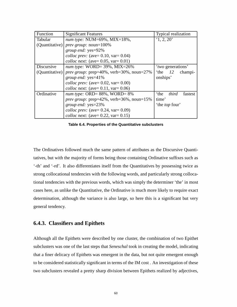
Function Significant Features Typical realizationTabular(Quantitative)
num type: NUM=69%, MIX=18%,prev group: noun=100%group end: yes=92%colloc prev: (ave= 0.10, var= 0.04)colloc next: (ave= 0.05, var= 0.01)
‘1, 2, 20’
Discursive(Quantitative)
num type: WORD= 39%, MIX=26%prev group: prep=40%, verb=30%, noun=27%group end: yes=41%colloc prev: (ave= 0.02, var= 0.00)colloc next: (ave= 0.11, var= 0.06)
‘two generations’‘the 12 champi-onships’
Ordinative num type: ORD= 88%, WORD= 8%prev group: prep=42%, verb=36%, noun=15%group end: yes=23%colloc prev: (ave= 0.24, var= 0.09)colloc next: (ave= 0.22, var= 0.15)
‘the third fastesttime’‘the top four’
Table 6.4. Properties of the Quantitative subclusters
The Ordinatives followed much the same pattern of attributes as the Discursive Quanti-
tatives, but with the majority of forms being those containing Ordinative suffixes such as
‘-th’ and ‘-rd’. It also differentiates itself from the Quantitatives by possessing twice as
strong collocational tendencies with the following words, and particularly strong colloca-
tional tendencies with the previous words, which was simply the determiner ‘the’ in most
cases here, as unlike the Quantitative, the Ordinative is much more likely to require exact
determination, although the variance is also large, so here this is a significant but very
general tendency.
6.4.3. Classifiers and Epithets
Although all the Epithets were described by one cluster, the combination of two Epithet
subclusters was one of the last steps that Seneschal took in creating the model, indicating
that a finer delicacy of Epithets was emergent in the data, but not quite emergent enough
to be considered statistically significant in terms of the IM cost . An investigation of these
two subclusters revealed a pretty sharp division between Epithets realized by adjectives,
60
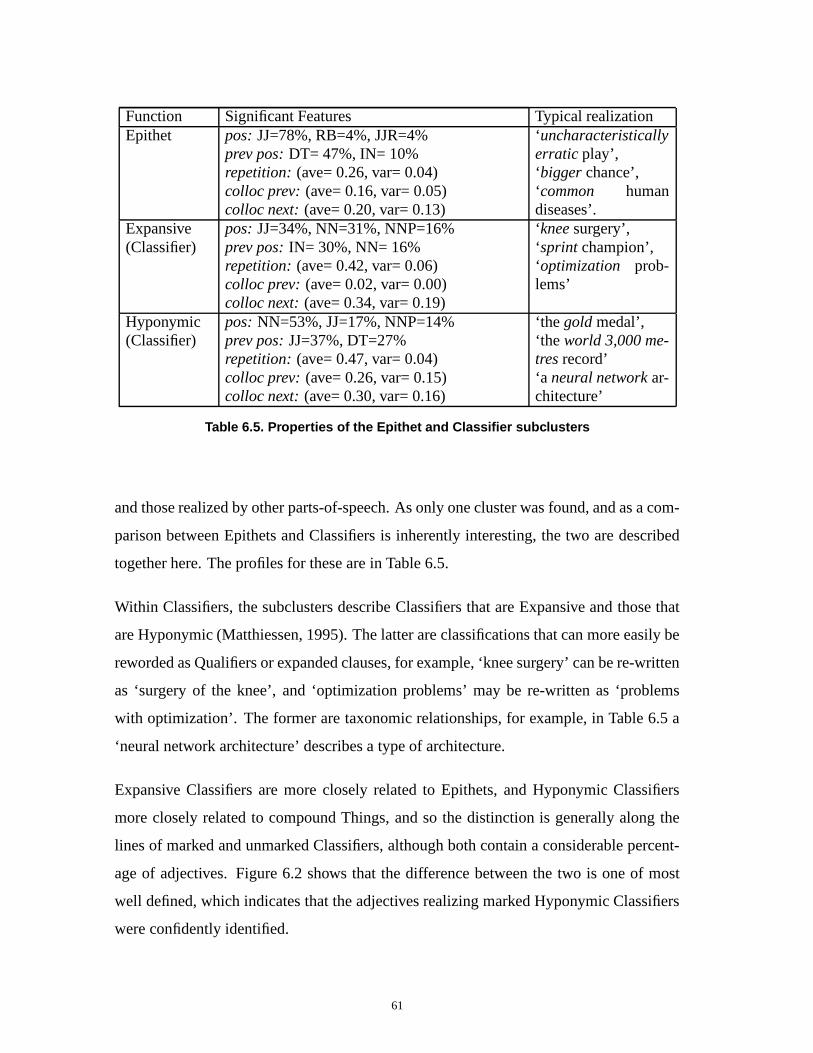
Function Significant Features Typical realizationEpithet pos: JJ=78%, RB=4%, JJR=4%
prev pos: DT= 47%, IN= 10%repetition: (ave= 0.26, var= 0.04)colloc prev: (ave= 0.16, var= 0.05)colloc next: (ave= 0.20, var= 0.13)
‘uncharacteristicallyerratic play’,‘bigger chance’,‘common humandiseases’.
Expansive(Classifier)
pos: JJ=34%, NN=31%, NNP=16%prev pos: IN= 30%, NN= 16%repetition: (ave= 0.42, var= 0.06)colloc prev: (ave= 0.02, var= 0.00)colloc next: (ave= 0.34, var= 0.19)
‘knee surgery’,‘sprint champion’,‘optimization prob-lems’
Hyponymic(Classifier)
pos: NN=53%, JJ=17%, NNP=14%prev pos: JJ=37%, DT=27%repetition: (ave= 0.47, var= 0.04)colloc prev: (ave= 0.26, var= 0.15)colloc next: (ave= 0.30, var= 0.16)
‘the gold medal’,‘the world 3,000 me-tres record’‘a neural network ar-chitecture’
Table 6.5. Properties of the Epithet and Classifier subclusters
and those realized by other parts-of-speech. As only one cluster was found, and as a com-
parison between Epithets and Classifiers is inherently interesting, the two are described
together here. The profiles for these are in Table 6.5.
Within Classifiers, the subclusters describe Classifiers that are Expansive and those that
are Hyponymic (Matthiessen, 1995). The latter are classifications that can more easily be
reworded as Qualifiers or expanded clauses, for example, ‘knee surgery’ can be re-written
as ‘surgery of the knee’, and ‘optimization problems’ may be re-written as ‘problems
with optimization’. The former are taxonomic relationships, for example, in Table 6.5 a
‘neural network architecture’ describes a type of architecture.
Expansive Classifiers are more closely related to Epithets, and Hyponymic Classifiers
more closely related to compound Things, and so the distinction is generally along the
lines of marked and unmarked Classifiers, although both contain a considerable percent-
age of adjectives. Figure 6.2 shows that the difference between the two is one of most
well defined, which indicates that the adjectives realizing marked Hyponymic Classifiers
were confidently identified.
61

Hyponymic Classifiers are much more likely to occur in compound or recursive Classify-
ing structures, which is why they exhibit strong collocational tendencies with the previous
word, while the Expansive Classifiers exhibit next to none. As should be expected, the
collocational tendencies with the following word was greater for Classifiers than for Epi-
thets (between 50%-70% more here), although the variance is also quite large.
The parts-of-speech of previous words also differs. While the Hyponymic Classifiers
seem to follow adjectives, and therefore are likely to follow other Classifiers or Epithets,
the Expansive Classifiers most commonly follow a preposition, indicating that they are
likely to occur without a Deictic.
Most interestingly, the probability of a Classifier being repeated within a document was
almost twice as much as that for Epithets, which is especially significant when it is con-
sidered that the words realizing Epithets are generally more frequent. As the variance
is low, this relatively simple feature seems to be a good factor in the disambiguation of
function. The reasons for these are those given in Chapter 3: Classifiers are less likely to
be dropped from the group when the Thing is repeated and terms realizing Classifiers are
more likely to also be used metonymically or as the Thing.
6.4.4. Thing
Within the rank of term, Things typically, (but not always) function as the semantic Head
of the group, so they do not so much function as simply ‘exist’, as compared to the rest of
the nominal group. Nonetheless, the representation and classification of finer delicacies
of Thing was a significant result in this study, with less than one third the error of an
unmarked classification (see Table 6.10), and the discovery of seven subclusters / levels
of delicacy.
In most texts, when Things (or nouns) are divided into subtypes, the most common divi-
sions made are between countable and non-countable nouns. There is no such divisions
apparent in the Thing subclusters here. This may be because one grammatical device
62

Function Significant Features Typical realizationFirst Name(Thing)
group start: yes=96%pos: NNP=94%, JJ= 2%prev group: noun=81%, prep=8%, conj=6%next group: noun=69%, verb=13%, prep=10%colloc prev: (ave= 0.03, var= 0.01)colloc next: (ave= 0.48, var= 0.18)
Joel,Lance,Despina,Atul,Mr.
Intermediary(Thing)
group start: yes=0%pos: NNP=88%, NNS=5%,prev group: prep=55%, noun=28%, conj=6%next group: noun=58%, prep=20%, verb=15%colloc prev: (ave= 0.27, var= 0.13)colloc next: (ave= 0.46, var= 0.17)
World,de,Open,PGA
Last Name(Thing)
group start: yes=0%pos: NNP= 94%, NNPS= 5%,prev pos: noun=65%, prep=22%, verb=6%next group: noun=62%, prep=15%, verb=14%colloc prev: (ave= 0.46, var= 0.18)colloc next: (ave= 0.01, var= 0.00)
Slam,Komen,Olympics,Stromberg
Table 6.6. Properties of the Named Entity Things
for quantifying non-countable nouns, the pre-Numerative, was quite rare, or because they
simply weren’t captured in the feature space.
The subclusters that were discovered can be roughly divided between those describing
named entities, those with the group realized by one word and nominals that are best
described in terms of how they are modified. This is how they are divided in Tables 6.6,
6.7 and 6.8 respectively.
In Table 6.6, the subclusters roughly conformed to simple word order, as Proper nouns
typically do, with rough divisions between initial, intermediary and final words in named
entity complexes, simply labelled First Name, Intermediary and Last Name here. Included
in the Intermediary group are forms that are initial but commonly take a Deictic, such as
’the United States’. Not reported in Table 6.6 is the understandable probability that a
First Name is only about half as likely to be repeated in a document as a Last Name.
No satisfactory explanation was found that explained why named entities containing an
intermediary where very significantly more likely to follow a prepositional group. One
63

Function Significant Features Typical realizationNominative(Thing)
group start: yes=93.7%pos: NNP= 46%, PRP= 28%, WP=8%prev punc: period=26%, comma=26% and/orinverted commas=10%, left parenthesis=4%prev group: noun=97%, verb=2%repetition: (ave= 0.58, var= 0.06)colloc prev: (ave= 0.03, var= 0.01)
‘He then clocked’,‘I’m sure’,‘Clignet has’
non-Nominative(Thing)
group start: yes=100%pos: NNP=27%, PRP=26%, NN=16%,prev punc: period=4%, comma=3%, and/or in-verted commas=3%prev group: p= 50%, v= 32%, c= 12%repetition: (ave= 0.49, var= 0.08)colloc prev: (ave= 0.11, var= 0.04)
‘of Denmark’,‘going to Britain’,‘in danger’
Table 6.7. Properties of the Group-Realising Things
suggestion that can be made is that the occurrence of a Deictic indicates that the entity
is an organisation or country, not a person, and are therefore more likely to be used in
speech such as ’the person from/of the United States’, although this does not account for
all cases here.
The collocational tendencies followed the expected patterns. The exploitation of these
enabled the system to distinguish between a named entity functioning as a Hyponymic
Classifier and one functioning as the beginning of a compound Thing, as in ‘the Brussels
Grand Prix’, as did the fact that ‘Brussels’ was very likely to be repeated in this context,
and therefore less likely to be the First Name in an entity complex. This was significantly
more accurate than the unmarked classification, which was unable to distinguish these
cases.
In Table 6.7, the group realizing delicacies within Thing are given. For over 90% of cases,
both the Nominative and non-Nominative realize the entire nominal group. The ‘Nomina-
tive’ Things are much more likely to occur in the Subject position, the ‘non-Nominative’
Things in any other. Although there where no features that explicitly describing this dif-
ference, some evidence may be seen with the relative frequency of previous punctuation,
knowledge of the previous group, and the prevalence of ‘who’.
64
The remaining two Things, given in Table 6.8 are the most interesting and hardest to
identify from purely the feature space or forms themselves. Given the similarity in their
feature space, it is difficult to see why these two weren’t combined, while the two Epithet
subclusters were. This is probably a good example of how intuition about what divisions
exist may bias what is really emergent in the data with respect to the features used, as
there obviously was some reason for distinguishing the two, even if this was a slight but
consistent variation over a large number of features.
As Table 6.8 shows, this difference is not particularly emergent in the features space,
although the high percentage of neighbouring nominal groups for the Described Thing
indicates that they may be more likely to occur as part of a nominal group complex. The
Functions were named according the variation in the choice of modification. The differ-
ence between the two is most emergent when the function of modification is considered.
Figure 6.3 shows the relative frequencies of the functions of the terms immediately pre-
ceding Stated and Described Things4.
The Stated and Described Things correspond very closely to the Referring and Informing
functions of the nominal group, and it would be interesting to explore whether Things that
are of similar probability of being Stated and Described are realized in the conflation of
Referring and Informing functions, as described in (O’Donnell, 1998).
The distinction between the two may be seen in the choices made within the Deictic and
Classification systems of delicacy. While the Stated is twice as likely to be modified by
a Deictic, over 80% of these are Demonstratives, which don’t feature in the Described’s
modifications at all. This trend is reversed for Classifiers. The Described Things are more
than twice as likely to be modified by a Classifier, and within this over 70% of cases are
Expansive, as opposed to about 25% for the Stated Things.
As Figure 6.2 shows, the general trend of the Hyponymic Classifiers being more closely
related to the Thing is reversed for the Stated Things, that is, a Stated thing is more closely
related to an Expansive Classifier than a Hyponymic Classifier. One explanation is that
4The percentages in Figure 6.3 for the Described Things taken from only the 42% that were pre-modified
65

Function Significant Features Typical realizationStated(Thing)
group start: yes=2%pos: NN= 67%, NNS=30%prev pos: JJ= 32%, DT= 27%, NN= 16%prev group: prep=46%, verb=33%, noun=12%next group: prep=45%, noun=21%, verb=10%colloc prev: (ave= 0.31, var= 0.16)colloc next: (ave= 0.08, var= 0.02)
‘media questions’,‘the invitation’,‘such comparisons’
Described(Thing)
group start: yes=58%pos: NN= 45%, NNS=13%prev pos: J= 21%, NN= 21%, NNP= 19%prev group: noun=78%, verb=12%, prep=8%next group: noun=91%, verb=4%, conj=2%colloc prev: (ave= 0.10, var= 0.05)colloc next: (ave= 0.01, var= 0.00)
‘20.67 seconds’,‘former winner’,‘our implementation’
Table 6.8. Properties of the nominal Things
it represents the fact that a Hyponymic Classifier may itself undergo Classification, while
an Expansive Classifier generally does not, although the Stated thing seems to define
a number of aberrant ‘hills and valleys’ with the intersection of the Epithet, Classifier
and Thing functions in Figure 6.2, indicating it may represent something much more
fundamental.
Not described in Figure 6.3 is that the percent of Epithets is much less than the percent-
age of preceding adjectives given in Table 6.8, indicating that markedness is common to
both. The fact that the ‘Stated’ is twice as likely as the ‘Described’ to be modified Epi-
thetically indicates that the labels given to them are not quite sufficient in describing the
complexities of the differences, but regardless of how well the functions of the delicacies
are described by the labels given, the existence of the subclusters and significant variances
in Figure 6.3 are unchanged. This also demonstrates that at finer layers of delicacy, the
variation in function can quickly become very emergent, even when the corresponding
parts-of-speech and other surface-level phenomena differ only slightly.
66
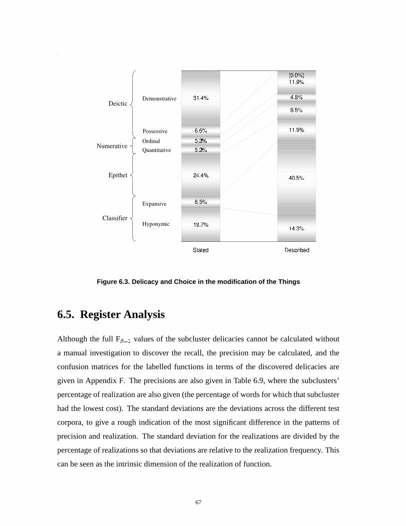
Figure 6.3. Delicacy and Choice in the modification of the Things
6.5. Register Analysis
Although the full F� ���
values of the subcluster delicacies cannot be calculated without
a manual investigation to discover the recall, the precision may be calculated, and the
confusion matrices for the labelled functions in terms of the discovered delicacies are
given in Appendix F. The precisions are also given in Table 6.9, where the subclusters’
percentage of realization are also given (the percentage of words for which that subcluster
had the lowest cost). The standard deviations are the deviations across the different test
corpora, to give a rough indication of the most significant difference in the patterns of
precision and realization. The standard deviation for the realizations are divided by the
percentage of realizations so that deviations are relative to the realization frequency. This
can be seen as the intrinsic dimension of the realization of function.
67

Corpus Reuters-A Reuters-B BIO-INF MOD-FIC Overallsubcluster prec. rls. prec. rls. prec. rls. prec. rls. prec. & � rls. & � /rls.
Demon 100% 13% 99% 15% 85% 10% 99% 20% 96% 7% 14% 29%Poss 97% 6% 96% 6% 78% 2% 100% 4% 94% 10% 4% 44%
Ord 66% 3% 82% 3% 0% 0% 71% 1% 71% 37% 2% 92%Disc 85% 5% 87% 3% 52% 1% 50% 1% 74% 20% 3% 74%Tabular 100% 0% 100% 1% 82% 3% n/a 0% 87% 10% 1% 105%
Epithet 63% 4% 64% 3% 60% 6% 84% 6% 67% 11% 5% 33%Expans 36% 1% 25% 1% 80% 4% 30% 1% 51% 25% 2% 92%Hypon 73% 5% 58% 4% 91% 8% 43% 1% 73% 21% 5% 58%
F Name 95% 6% 93% 5% 91% 5% 100% 1% 93% 4% 4% 58%I Name 85% 2% 79% 2% 91% 1% 100% 0% 85% 9% 1% 49%L Name 100% 9% 98% 8% 100% 5% 100% 1% 99% 1% 6% 58%Nom 98% 7% 100% 7% 98% 5% 100% 6% 99% 1% 6% 15%non-Nom 97% 10% 92% 9% 93% 8% 97% 24% 95% 3% 12% 60%Stated 99% 17% 97% 18% 99% 24% 99% 26% 98% 1% 21% 21%Descr 88% 3% 88% 3% 100% 6% 100% 2% 96% 7% 4% 49%
Table 6.9. Subcluster Precisions and Percent of realization
These patterns provide a good description of how register variation is emergent in the
utilisation of the grammar. Here, Reuters-A and Reuters-B exhibit an almost identical
pattern of realization across all functions.
Within Deictics, The Bio-Inf’s were more difficult to identify, and taking into account the
lower precisions, were significantly less frequent than in the other registers. The Mod-Fic
Demonstratives were more frequent, especially in relation to the Possessives, which were
only realized in large numbers in the Reuters corpora, predominantly within extensive
Genitive phrases.
Although they were relatively infrequent, the greatest variance in both precision and re-
alization occurred within the Numerative and Classifier functions. Numeratives were
almost absent from the Bio-Inf and Mod-Fic corpora. The high number of Tabular Quan-
titatives in the Bio-Inf corpus were predominantly realized by header information such as
the volume number, date of publication and footnote indicators. Referring to Tables E.3
E.2 E.5 and E.4 for the recall values for the Ordinative, both the Bio-Inf and Mod-Fic reg-
isters obtained 100% recall for Ordinatives, while the Reuters registers were significantly
lower, which is a product of some marked Classifiers such as ‘1st prize’ being missclassi-
fied as Ordinatives. Such marked functions were predictably absent from the non-sports
registers. Where the Bio-Inf corpus lost accuracy was between the Numeratives and the
68

Function Unmarked Classification Gain / Lossrecall precision F
� ���recall precision F
� ���F� ���
Deictic 97.7% 96.2% 0.969 97.5% 95.5% 0.965 � 0.005Quantifier 90.8% 56.4% 0.696 73% 78% 0.755
�0.059
Ordinative 80.3% 71% 0.754 77% 71.2% 0.740 � 0.014Epithet 79.9% 55.4% 0.655 67.2% 66.5% 0.668
�0.014
Classifier 60.1% 48.7% 0.538 65% 66% 0.655�
0.117Thing 81% 98.9% 0.891 96.5% 96.8% 0.967
�0.076
Table 6.10. Overall: Comparison with Unmarked Function
Deictics, with a greater frequency of numbers realizing Deictics in phrase such as ‘one
previous attempt’.
The very low realization and precision for Classifiers in the Mod-Fic register indicates
that there were almost no Classifiers at all, but a fair number of Epithets and Things were
missclassified as Classifiers. This can be seen as evidence of the domain dependence of
learning from a very different register. In general though, the accuracies for this register
were quite high, with Epithets being both the most frequent and most accurately classified.
This seems to be because the narrative describes the fleeting thoughts of a group of people
in the early part of the day, so perhaps it is simply the breakfast table of modernism that
is largely unmarked.
It is in the Bio-Inf register that Classifiers were both more frequently realized and more
successfully identified. As stated in Section 5.1, the former was expected, the latter was
not. A good explanation for why the Expansive Classifiers in particular were correctly
identified is not easily found. It may be that the authors, consciously or unconsciously
aware that the Classifier structures were both complex and marked, deliberately chose to
represent these as unambiguously as possible. This is quite likely, as the corpus was taken
from abstracts, which are (or at least should be) summations of the main text created with
just this in mind.
The relatively smaller groups of the Mod-Fic corpus can be seen in the frequency of
realization of the group-realizing Things. It is only the non-Nominative that are more
frequent, indicating that the groups realizing the Subjects are no more likely to be realized
69
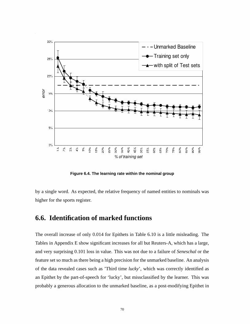
Figure 6.4. The learning rate within the nominal group
by a single word. As expected, the relative frequency of named entities to nominals was
higher for the sports register.
6.6. Identification of marked functions
The overall increase of only 0.014 for Epithets in Table 6.10 is a little misleading. The
Tables in Appendix E show significant increases for all but Reuters-A, which has a large,
and very surprising 0.101 loss in value. This was not due to a failure of Seneschal or the
feature set so much as there being a high precision for the unmarked baseline. An analysis
of the data revealed cases such as ’Third time lucky’, which was correctly identified as
an Epithet by the part-of-speech for ‘lucky’, but missclassified by the learner. This was
probably a generous allocation to the unmarked baseline, as a post-modifying Epithet in
70

English is very marked. Within Reuters-A, this was compensated for by a 0.181 increase
for Classifiers.
6.7. Learning Rate and Domain Dependence
Figure 6.4 gives the learning rate of the nominal group for the two sets of tests defined in
Section 5.3.
Using only the Reuters training set, an accurate grammar was inferred very quickly, cross-
ing the unmarked baseline of 17.4% error with only 5% of the training set (about 140
words). The introduction of training items from the same registers as the test sets gave
more accurate results, but only about 2% better, showing that the grammar learned was
quite robust despite the substantial variations between registers.
If the curve is a good indication, it seems that the accuracies reported in Table 6.2 were
about the highest achievable result for function within the nominal group for this study,
with respect to corpus size and this feature set, as both gain very little after about 50% of
the data is seen.
71

CHAPTER 7
Concluding Remarks
It has been demonstrated that a probabilistic representation of a functional grammar is
possible such that it is inferred from labelled text by a supervised mixture modeller, and
that such a representation may be used to accurately give functional classifications to
unlabelled text.
It has further been demonstrated that supervised mixture modelling can perform as accu-
rately as current state-of-the-art machine learning algorithms across many data sets, and
is a linearly scalable solution to the Bayes attribute independence assumption.
The most significant outcome here is the level of sophistication in the discovery of the
more delicate functions. As these were found through unsupervised methods the possibil-
ity of applying these methods over much larger scales is very real. Especially within the
Things, the significance of the following and previous group’s functions were much higher
than might be expected. Such methods could be used within any theory of language, and
even seem to correspond to Whorf’s notions of covert categories or ‘cryptotypes’ (Whorf,
1956) as there are significant tendencies in the type of modification they underwent and
the contexts in which they were typically used.
This thesis has presented a methodology for learning and representing a functional lexi-
cogrammar that can be applied and build upon in a variety of ways.
A further and not very difficult extension of the study to semi-supervised learning might
provide a good middle-ground between the supervised and unsupervised techniques used
here. It may also overcome the (small) amount of register dependence that was observed.
There were a number of features that were not included in the final testing but were either
theorised or demonstrated to be useful. The exploration of these and potentially many
72

more types of features would no doubt lead to more accurate representations and different
discoveries of delicacy.
Rich sources of linguistic information are available from the system described here, in-
cluding the functions themselves, levels of delicacy, significant features, register varia-
tions and the patterns of choice and realization. These could be utilised in a number of
tasks in Natural Language Processing and Computational Linguistics. Hopefully, the re-
sults have demonstrated that not only can computational methods increase the scale of a
study, they can also be an active participant in the analysis of language.
73

References
C.C. Aggarwal, A. Hinneburg, and D.A. Keim. 2001. On the surprising behavior of
distance metrics in high dimensional space. In Proceedings of the 8th International
Conference on Database Theory (ICDT’01),.
J.A. Bateman and E. Teich. 1991. SFG and HPSG: An attempt to reconcile a functional
and an information-based view on grammar. In in Proceedings of the Workshop on
Head-Driven Phrase Structure Grammar, Saarbruecken.
J.A. Bateman, R.T. Kasper, J.F.L. Schütz, and E.H. Steiner. 1989. A new view on
the translation process. In Proceedings of the European Chapter of the Association for
Computational Linguistics, Manchester, England. April, 1989. Association for Com-
putational Linguistics.
J.A. Bateman, M. Emele, and S. Momma. 1992a. The nondirectional representation
of Systemic Functional Grammars and Semantics as Typed Feature Structures. In
Proceedings of COLING-92, volume 3, pages 916–920.
J.A. Bateman, E. Maier, C.M.I.M. Matthiessen, and C. Paris. 1992b. Generation
systems design: Issues of modularity. Technical report, GMD, Integrated Publication
and Information Systems Institute, Darmstadt, Germany. forthcoming.
J.A. Bateman. 1992. Grammar, systemic. In S. Shapiro, editor, Encyclopedia of
Artificial Intelligence, Second Edition, pages 583–592. John Wiley and Sons, Inc.
Adam L. Berger, Stephen A. Della Pietra, and Vincent J. Della Pietra. 1996. A max-
imum entropy approach to Natural Language Processing. Computational Linguistics,
22(1):39–71.
P. Berkhin. 2002. Survey of clustering data mining techniques. Accrue Software.
74

P. Bhattacharyya, V. Sindhwani, and S. Rakshit. 2001. Information theoretic feature
crediting in multiclass support vector machines. In Proceedings of the first SIAM In-
ternational Conference on Data Mining.
B. Bohnet, S. Klatt, and L. Wanner. 2002. A bootstrapping approach to automatic
annotation of functional information to adjectives with an application to German. In
Proceedings of the Third International Conference On Language Resources And Eval-
uation (LREC2003).
M.R. Brent and T.A. Cartwright. 1997. Distributional regularity and phonotactic con-
straints are useful for segmentation. In M.R. Brent, editor, Computational Approaches
to Language Acquisition. MIT Press.
J. Bresnan. 2001. Lexical-Functional Syntax. Blackwell, Oxford.
H. Bunt and A. Nijholt. 2000. New parsing technologies. In Advances in Probabilistic
and Other Parsing Technologies. Kluwer Academic Publishers, Dordrecht.
X. Carreras and Lu. Màrquez. 2001. Boosting trees for clause splitting. In Wal-
ter Daelemans and Rémi Zajac, editors, Proceedings of CoNLL-2001, pages 73–75.
Toulouse, France.
N. Chomsky. 1957. Syntactic Structures. Mouton & Co, The Hague.
N. Chomsky. 1965. Aspects of the theory of syntax. M.I.T. Press, Cambridge.
N. Chomsky. 1986. Knowledge of language: Its nature, origin, and use. Praeger, New
York.
M. Collins. 1999. Head-Driven Statistical Models for Natural Language Parsing.
Ph.D. thesis, University of Pennsylvania.
F.G. Cozman, I. Cohen, and M.C. Cirelo. 2003. Semi-supervised learning of mixture
models and bayesian networks. In Proceedings of the Twentieth International Confer-
ence of Machine Learning.
M. Cross. 1993. Collocation in computer modelling of lexis as most delicate grammar.
In M. Ghadessy, editor, Registers of Written English, pages 196–220. Pinter Publishers,
London.
75

T.G. Dietterich. 1998. Machine-learning research: Four current directions. The AI
Magazine, 18(4):97–136.
S.C. Dik. 1981. Functional grammar. Foris, Dordrecht.
S.C. Dik. 1992. Functional Grammar in Prolog: an integrated implementation for
English, French, and Dutch. Mouton de Gruyter, Berlin/New York.
M. Dowman. 2002. Modelling the Acquisition of Colour Words. Springer-Verlag,
Canberra.
G. Escudero, L. Marquez, and G. Rigau. 2000. An empirical study of the domain
dependence of supervised word sense disambiguation systems. In in Proceedings of
Joint SIGDAT Conference on Empirical Methods in Natural Language Processing and
Very Large Corpora (EMNLP/VLC’00).
R.P. Fawcett. 2000. A theory of syntax for systemic functional linguistics. John Ben-
jamins, Amsterdam.
A. Frank, T.H. King, and J. Kuhn. 2001. Optimality Theory style constraint rank-
ing in large-scale LFG grammars. In P. Sells, editor, Formal and empirical issues in
optimality theoretic syntax. CSLI Publications, Stanford.
J. Goodman. 2000. Probabilistic feature grammars. In Advances in Probabilistic and
Other Parsing Technologies. Kluwer Academic Publishers, Dordrecht.
M.A.K. Halliday and C.M.I.M. Matthiessen. 1999. Construing experience through
meaning: a language-based approach to cognition. Cassell, London.
M.A.K. Halliday. 1978. Language as a Social Semiotic. University Park Press.
M.A.K. Halliday. 1985. An Introduction to Functional Grammar. Edward Arnold,
London.
M.A.K. Halliday. 2002. On Grammar. Continuum, London.
R. Hasan. 1987. The grammarians dream: lexis as most delicate grammar. In M.A.K.
Halliday and R.R. Fawcett, editors, New Developments in Systemic Linguistics, Vol 1:
Theory and Description. Pinter, London.
76

M.A. Hearst. 1998. Automated discovery of WordNet relations. In C. Fellbaum,
editor, WordNet: an Electronic Lexical Database. MIT Press, Cambridge MA.
M. Herke-Couchman and C. Whitelaw. 2003. Identifying interpersonal distance us-
ing systemic features. In Proceedings of the First Australasian Language Technology
Workshop (ALTW2003).
R. Iyer and M. Ostendorf. 1996. Modeling long distance dependence in language:
Topic mixtures vs. dynamic cache models. In Proc. ICSLP ’96, volume 1, pages 236–
239, Philadelphia, PA.
J.R. Jang, C.T. Sun, and E. Mizutani. 1997. Neuro-Fuzzy and Soft Computing: A
computational approach to learning and machine intelligence. Prentice Hall.
R. Kasper. 1988. An experimental parser for Systemic Grammars. In Proceedings
of the 12th International Conference on Computational Linguistics. Association for
Computational Linguistics.
A. Knott, T. Sanders, and J. Oberlander. 2001. Levels of representation in discourse
relations. Cognitive Linguistics, 12(3):197–209.
R. Kohavi. 1996. Scaling up the accuracy of Naive-Bayes classifiers: a decision-
tree hybrid. In Proceedings of the Second International Conference on Knowledge
Discovery and Data Mining.
J. Kuhn. 2001. Generation and parsing in optimality theoretic syntax. In P. Sells,
editor, Formal and empirical issues in optimality theoretic syntax. CSLI Publications,
Stanford.
S. Kullback. 1959. Information theory and statistics. John Wiley, New York.
R.A. Olshen L. Breiman, J.H. Friedman and C.J. Stone. 1984. Classification and
Regression Trees. Chapman & Hall.
Peter Lane and James Henderson. 2001. Incremental syntactic parsing of natural
language corpora with simple synchrony networks. Knowledge and Data Engineering,
13(2):219–231.
77

S. Lawrence, C.L. Giles, and S. Fong. 2000. Natural language grammatical inference
with recurrent neural networks. IEEE Transactions on Knowledge and Data Engineer-
ing, 12(1):126–140.
G. Legendre, J. Grimshaw, and S. Vikner, editors. 2001. Optimality-theoretic syntax.
MIT Press, Cambridge.
D.D. Lewis. 1998. Naive (Bayes) at forty: The independence assumption in infor-
mation retrieval. In Claire Nédellec and Céline Rouveirol, editors, Proceedings of
ECML-98, 10th European Conference on Machine Learning, number 1398, Chemnitz,
DE. Springer Verlag, Heidelberg, DE.
H. Li and N. Abe. 1998. Word clustering and disambiguation based on co-occurence
data. In COLING-ACL, pages 749–755.
O. L. Mangasarian and D. R. Musicant. 2001. Lagrangian support vector machines.
Journal of Machine Learning Research, 1:161–177.
W. Mann and C.M.I.M. Mattheissen. 1985. A demonstration of the nigel text genera-
tion computer program. In J. D. Benson and W. S. Greaves, editors, Systemic Perspec-
tives on Discourse, volume 1, pages 84–95. Ablex, Norwood, NJ.
C.D. Manning and H. Schütze. 1999. Foundations of Statistical Natural Language
Processing. The MIT Press, Cambridge, Massachusetts.
L. Màrquez. 2000. Machine Learning and Natural Language Processing. Technical
Report LSI-00-45-R, Departament de Llenguatges i Sistemes Informàtics (LSI), Uni-
versitat Politecnica de Catalunya (UPC), Barcelona, Spain.
D. Martinez and E. Agirre. 2000. One sense per collocation and genre/topic variations.
In in Proceedings of the Joint SIGDAT Conference on Empirical Methods in Natural
Language Processing and Very Large Corpora.
C.M.I.M. Matthiessen and J. A. Bateman. 1991. Text Generation and Systemic-
Functional Linguistics. Communication in Artificial Intelligence Series. Pinter, Lon-
don.
78

C.M.I.M. Matthiessen, M. O’Donnell, and L. Zeng. 1991. Discourse analysis and the
need for functionally complex grammar in parsing. In Proceedings of the 2nd Japan-
Australia Joint Symposium on Natural Language Processing, Kyushu, Japan. Kyushu
Institute of Technology.
C.M.I.M. Matthiessen. 1983. The systemic framework in text generation: Nigel.
USC/Information Sciences Institute.
C.M.I.M. Matthiessen. 1995. Lexicogrammatical cartography: English systems. In-
ternational Language Science Publishers, Tokyo, Taipei and Dallas.
C.M.I.M. Matthiessen. 1997. Glossary of Systemic Functional terms.
[http://minerva.ling.mq.edu.au/resource/VirtuallLibrary/Glossary/sysglossary.htm].
Macquarie University.
J.J. McCarthy and A.S. Prince. 1995. Faithfulness and reduplicative identity. In
J.N. Beckman, L.W. Dickey, and S. Urbanczyk, editors, Papers in optimality theory
University of Massachusetts Occasional Papers 18. GLSA, Amherst.
G.J. McLachlan and D. Peel. 2000. Finite Mixture Models. Wiley.
C.J. Merz and P.M. Murphy. 1996. UCI repository of machine learning databases.
G.A. Miller, R. Beckwith, C. Fellbaum, D. Gross, and K.J. Miller. 1990. Introduction
to WordNet: An on-line lexical database. Journal of Lexicography, 3(4):235–244.
D.I. Moldovan and R. Girju. 2001. An interactive tool for the rapid development of
knowledge bases. International Journal on Artificial Intelligence Tools, 10(1-2):65–
86.
R. Munro. 2003a. A queuing-theory model for word frequency distributions. In
Proceedings of the First Australasian Language Technology Workshop (ALTW2003).
R. Munro. 2003b. Seneschal: classification and analysis in supervised mixture-
modelling. In Proceedings of the Third International Conference on Hybrid Intelligent
Systems (HIS’03). IOS Press.
79

T. Oates, T. Armstrong, J. Harris, and M. Nejman. 2003. Leveraging lexical seman-
tics to infer context-free grammars. In 7th European Conference on Principles and
Practice of Knowledge Discovery in Databases (PKDD).
M. O’Donnell. 1994. Sentence analysis and generation: a systemic perspective. Ph.D.
thesis, University of Sydney, Department of Linguistics, Sydney, Australia.
M O’Donnell. 1998. Integrating referring and informing in NP planning. In Proceed-
ings of the Coling-ACL ’98 Workshop on the Computational Treatment of Nominals.
M. O’Donnell. 2002. Automating the coding of semantic patterns: applying machine
learning to corpus linguistics. In Proceedings of 29th International Systemic Func-
tional Workshop.
T.F. O’Donoghue. 1991. A semantic interpreter for systemic grammars. In Proceed-
ings of the ACL workshop on Reversible Grammars, Berkeley, California. Association
for Computational Linguistics.
J.J. Oliver. 1993. Decision graphs - an extension of decision trees. In Proceedings of
the Fourth International Workshop on Artificial Intelligence and Statistics.
F.C.N. Pereira, N. Tishby, and L. Lee. 1993. Distributional clustering of English
words. In Meeting of the Association for Computational Linguistics, pages 183–190.
C. Pollard and I.A. Sag. 1994. Head Driven Phrase Structure Grammar. University
of Chicago Press.
A. Prince and P. Smolensky. 1993. Optimality Theory: Constraint interaction in gener-
atire grammar. Technical Report TR-2, Rutgers University Cognitive Science Center,
New Brunswick.
F. Provost and P. Domingos. 2003. Tree induction for probability-based ranking.
Machine Learning, 52.
J.R. Quinlan. 1993. C4.5 – programs for machine learning. The Morgan Kaufmann
series in machine learning.
A. Ratnaparkhi. 1996. A maximum entropy part-of-speech tagger. In in Proceedings
of the Empirical Methods in Natural Language Processing Conference.
80

R. Rosenfeld. 2000. Two decades of statistical language modeling: Where do we go
from here. In Proceedings of the IEEE, volume 88.
H.S. Roy. 1995. Sharp, Reliable, Predictions Using Supervised Mixture Models.
Ph.D. thesis, Stanford University.
S. Rüeping. 2002. Incremental learning with support vector machines.
I.A. Sag, T. Baldwin, F. Bond, A. Copestake, and D. Flickinger. 2002. Multiword
expressions: A pain in the neck for nlp. In Proceedings of CICLING-2002. Springer.
C.G. Salas. 2001. Strategies for translating -ing adjectives and nouns from English to
Spanish. Translation Journal, 5(1).
J. Sinclair. 1991. Corpus, concordance, collocation. Oxford University Press.
D.C. Souter. 1996. A Corpus-Trained Parser for Systemic-Functional Syntax. Ph.D.
thesis, University of Leeds, School of Computer Studies.
A. Sperduti and A. Starita. 1997. Supervised neural networks for the classification of
structures. IEEE Transactions on Neural Networks, 8(3):714–735.
G. Thompson. 1999. Lexico-grammatical choices and contextual factors. In Mohsen
Ghadessy, editor, Text and Context in Functional Linguistics. J. Benjamins, Philadel-
phia.
G.H. Tucker. 1998. The Lexicogrammar of Adjectives: a systemic functional approach
to lexis. Functional Descriptions of Language Series. Cassell, London and New York.
R. Vilalta and Y. Drissi. 2002. A perspective view and survey of meta-learning. Jour-
nal of Artificial Intelligence Review, 18(2):77–95.
K. Wagstaff, C. Cardie, S. Rogers, and S. Schroedl. 2001. Constrained k-means clus-
tering with background knowledge. In Proceedings of the Eighteenth International
Conference on Machine Learning.
C.S. Wallace and D.M. Boulton. 1968. An information measure for classification.
Computer Journal, 11(2).
G.I. Webb and Z. Wang J. Boughton. 2002. Averaged One-Dependence Estimators:
Preliminary results. In Proceedings of the Australasian Data Mining Workshop.
81

B.L. Whorf. 1956. Grammatical categories. In J.B. Carroll, editor, Language Thought,
and Reality: Selected Writings of Benjamin Lee Worf. MIT Press.
D. Wolpert. 1995. Off-training set error and apriori distinctions between learning
algorithms. Technical Report 95–01–003, Santa Fe Institute.
Z. Zheng, G.I. Webb, and K.M. Ting. 1999. Lazy Bayesian rules: a lazy semi-naive
Bayesian learning technique competitive to boosting decision trees. In Proc. 16th In-
ternational Conf. on Machine Learning. Morgan Kaufmann, San Francisco, CA.
82

APPENDIX A
Glossary / Terminology
The meaning of many terms used in this work vary, and much of the terminology used is
specific to fields within semiotics, linguistics and computer science. There is the further
complication that this work covers a broad area. While linguists and semioticians will
probably be able to understand the machine learning concepts described here, SFG is rich
and comprehensive model of language, to describe it fully would require more than the
space of this thesis permits. A comprehensive SFG glossary is given in (Matthiessen,
1997).
Bootstrapping: A methodology in learning (typically for classification) that as-
sumes that an ordering of items is possible such that learning the earlier items
can inform and improve the learning of later items.
Class: The target category of a supervised learning task.
Classification: The ‘guessed’ class of an item in a supervised learning task.
Cluster: Any set of items taken from one data set.
Collocation / Concordance: The former is used as a blanket term for both here.
Delicacy: This describes the level of detail or granularity that a unit is defined in
terms of. In SFG, describing some unit at layers of delicacy will result make the
constraints of use more emergent.
Item / Instance / Row / data item: These refer to a single item in machine learn-
ing. In supervised learning, this will consist of that item’s class and its attributes.
Labelled / unlabelled data: Data items with/without known class memberships.
Marked / unmarked case: In linguistics the ‘unmarked’ case is the realization
that is expected, the marked case a realization that is unexpected, and typically
less common, although this will differ across registers.The unmarked case of a
83

function can loosely be thought of as the default case. For example, an Adjective
functioning as an Epithet is the unmarked case.
Multistate attributes: These are also known as discrete, multinomial and/or cate-
gorical attributes.
Rankshift / embedding: These essentially mean the same thing. It is the embed-
ding of a higher level of the grammatical hierarchy within a lower level.
Register / Domain: These refer to some specific type or genre of writing, each
term used more commonly in linguistics and language processing respectively.
Both are used here, but may be read synonymously.
Subcluster: Any cluster that contains items of only one class.
Topic Shift: Change in the subject matter of a text over time.
Training / test sets: Pre-labelled / unlabelled item sets in supervised learning.
84

APPENDIX B
Glossary of part-of-speech tags
(NB: Some of the terms used here, such as predeterminer do not necessarily match exactly
the functions defined in this thesis)
Token Part of SpeechCC Coordinating conjunctionCD Cardinal numberDT DeterminerEX ExistentialFW Foreign wordIN Preposition or subordinating conjunctionJJ AdjectiveJJR Adjective, comparativeJJS Adjective, superlativeLS List item markerMD ModalNN Noun, singular or massNNS Noun, pluralNNP Proper noun, singularNNPS Proper noun, pluralPDT PredeterminerPOS Possessive endingPRP Personal pronounPRP$ Possessive pronounRB AdverbRBR Adverb, comparativeRBS Adverb, superlativeRP ParticleSYM SymbolTO toUH InterjectionVB Verb, base formVBD Verb, past tenseVBG Verb, gerund or present participle
85

APPENDIX C
Confusion Matrices
C1. Adverb Group
classified as: A-pre Adv recallfunction:A-pre 4 1 80.0%Adv 0 11 100.0%precision 100.0% 91.7%
Table C.2. Adverb Group: Reuters-A
classified as: A-pre Adv recallfunction:A-pre 5 0 100.0%Adv 0 11 100.0%precision 100.0% 100.0%
Table C.3. Adverb Group: Reuters-B
classified as: A-pre Adv recallfunction:A-pre 1 0 100.0%Adv 0 11 100.0%precision 100.0% 100.0%
Table C.4. Adverb Group: Bio-Inf
classified as: A-pre Adv recallfunction:A-pre 1 1 50.0%Adv 0 42 100.0%precision 100.0% 97.7%
Table C.5. Adverb Group: Mod-Fict
86

C2. Conjunction Group
classified as: Conj C-pst recallfunction:Conj 25 0 100.0%C-pst 0 0 Quant/Advprecision 100.0% Quant/Adv
Table C.6. Conjunction Group: Reuters-A
classified as: Conj C-pst recallfunction:Conj 21 0 100.0%C-pst 0 0 Quant/Advprecision 100.0% Quant/Adv
Table C.7. Conjunction Group: Reuters-B
classified as: Conj C-pst recallfunction:Conj 51 0 100.0%C-pst 0 1 100.0%precision 100.0% 100.0%
Table C.8. Conjunction Group: Bio-Inf
classified as: Conj C-pst recallfunction:Conj 49 0 100.0%C-pst 0 1 100.0%precision 100.0% 100.0%
Table C.9. Conjunction Group: Mod-Fict
87

C3. Prepositional Group
classified as: P-pre Prep Pre-Deic recallfunction:P-pre 5 0 0 100.0%Prep 0 118 0 100.0%Pre-Deic 0 2 0 0.0%precision 100.0% 98.3% Quant/Adv
Table C.10. Prepositional Group: Reuters-A
classified as: P-pre Prep Pre-Deic recallfunction:P-pre 2 0 0 100.0%Prep 1 130 0 99.2%Pre-Deic 0 7 1 12.5%precision 66.7% 94.9% 100.0%
Table C.11. Prepositional Group: Reuters-B
classified as: P-pre Prep Pre-Deic recallfunction:P-pre 1 1 0 50.0%Prep 1 160 0 99.4%Pre-Deic 0 1 0 0.0%precision 50.0% 98.8% Quant/Adv
Table C.12. Prepositional Group: Bio-Inf
classified as: P-pre Prep Pre-Deic recallfunction:P-pre 2 0 1 66.7%Prep 0 143 0 100.0%Pre-Deic 0 4 0 0.0%precision 100.0% 97.3% 0.0%
Table C.13. Prepositional Group: Mod-Fict
88

C4. Nominal Group
classified as: Deic Quant Ord Epith Cfier Thing recallfunction:Deic 120 0 0 0 1 0 99.2%Quant 0 35 2 4 5 3 71.4%Ord 0 2 19 0 3 0 79.2%Epith 0 1 0 26 9 5 63.4%Cfier 1 0 3 9 40 3 71.4%Thing 0 3 5 2 4 352 96.2%precision 99.2% 85.4% 65.5% 63.4% 64.5% 97.0%
Table C.14. Nominal Group: Reuters-A
classified as: Deic Quant Ord Epith Cfier Thing recallfunction:Deic 148 0 0 1 3 0 97.4%Quant 1 29 0 2 4 7 67.4%Ord 0 0 23 2 5 1 74.2%Epith 0 0 3 23 11 3 57.5%Cfier 0 1 0 6 34 7 70.8%Thing 2 2 2 2 15 365 94.1%precision 98.0% 90.6% 82.1% 63.9% 47.2% 95.3%
Table C.15. Nominal Group: Reuters-B
classified as: Deic Quant Ord Epith Cfier Thing recallfunction:Deic 96 0 0 2 0 0 98.0%Quant 1 34 0 4 0 1 85.0%Ord 0 1 0 0 0 0 100.0%Epith 4 2 0 50 9 4 72.5%Cfier Poss 6 0 28 88 8 61.5%Thing 1 6 2 0 4 430 97.1%precision 83.5% 69.4% 0.0% 59.5% 87.1% 97.1%
Table C.16. Nominal Group: Bio-Inf
89

classified as: Deic Quant Ord Epith Cfier Thing recallfunction:Deic 143 1 0 0 5 0 96.0%Quant 1 5 0 0 3 0 55.6%Ord 0 0 5 0 0 0 100.0%Epith 0 3 0 38 6 7 70.4%Cfier 0 1 0 6 9 0 56.3%Thing 0 0 2 1 1 350 98.9%precision 99.3% 50.0% 71.4% 84.4% 37.5% 98.0%
Table C.17. Nominal Group: Mod-Fic
90

C5. Nominal Group Baselines
classified as: Deic Quant Ord Epith Cfier Thing recallfunction:Deic 121 0 0 0 0 0 100.0%Quant 0 44 4 0 0 1 89.8%Ord 1 5 16 1 0 0 69.6%Epith 0 6 0 32 3 0 78.0%Cfier 0 9 3 6 37 1 66.1%Thing 3 11 4 7 53 285 78.5%precision 96.8% 58.7% 59.3% 69.6% 39.8% 99.3%
Table C.18. Nominal Group Baseline: Reuters-A
classified as: Deic Quant Ord Epith Cfier Thing recallfunction:Deic 148 0 0 1 2 1 97.4%Quant 0 39 0 2 0 2 90.7%Ord 0 1 27 1 1 1 87.1%Epith 0 4 3 26 4 3 65.0%Cfier 0 0 0 11 36 1 75.0%Thing 4 Poss 3 11 59 298 76.8%precision 97.4% 68.4% 81.8% 50.0% 35.3% 97.4%
Table C.19. Nominal Group Baseline: Reuters-B
classified as: Deic Quant Ord Epith Cfier Thing recallfunction:Deic 95 0 0 3 0 0 96.9%Quant 0 37 0 2 0 1 92.5%Ord 0 1 0 0 0 0 100.0%Epith 0 5 0 57 7 0 82.6%Cfier 0 20 0 44 78 1 54.5%Thing 2 15 0 12 52 362 81.7%precision 97.9% 47.4% 0.0% 48.3% 56.9% 99.5%
Table C.20. Nominal Group Baseline: Bio-Inf
91
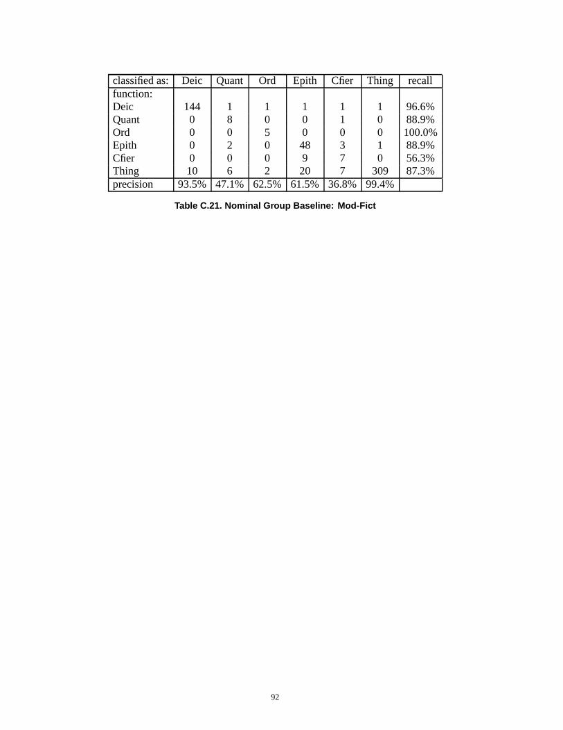
classified as: Deic Quant Ord Epith Cfier Thing recallfunction:Deic 144 1 1 1 1 1 96.6%Quant 0 8 0 0 1 0 88.9%Ord 0 0 5 0 0 0 100.0%Epith 0 2 0 48 3 1 88.9%Cfier 0 0 0 9 7 0 56.3%Thing 10 6 2 20 7 309 87.3%precision 93.5% 47.1% 62.5% 61.5% 36.8% 99.4%
Table C.21. Nominal Group Baseline: Mod-Fict
92

C6. Verb Group
classified as: Finite Aux Verb recallfunction:Finite 22 0 0 100.0%Aux 0 6 0 100.0%Verb 1 0 132 99.2%precision 95.7% 100.0% 100.0%
Table C.22. Verb Group: Reuters-A
classified as: Finite Aux Verb recallfunction:Finite 27 0 1 96.4%Aux 0 7 0 100.0%Verb 0 0 144 100.0%precision 100.0% 100.0% 99.3%
Table C.23. Verb Group: Reuters-B
classified as: Finite Aux Verb recallfunction:Finite 25 0 0 100.0%Aux 0 8 0 100.0%Verb 0 1 136 99.3%precision 100.0% 88.9% 100.0%
Table C.24. Verb Group: Bio-Inf
classified as: Finite Aux Verb recallfunction:Finite 36 0 10 78.3%Aux 0 6 1 85.7%Verb 3 1 196 98.0%precision 92.3% 85.7% 94.7%
Table C.25. Verb Group: Mod-Fict
93

APPENDIX D
Cost Matrices
cost: Deic Ord Quant Epith Cfier Thingfunction:Deic 17.6 33.4 31.9 29.8 28.0 30.5Ord 32.1 20.7 28.3 23.6 26.3 30.5Quant 35.7 30.2 21.2 33.6 30.5 29.1Epith 28.8 24.5 27.3 19.7 22.9 28.7Cfier 27.5 28.1 28.7 24.3 20.6 26.7Thing 33.8 32.3 33.2 32.0 30.2 21.0
Table D.2. Nominal Group Cost Matrix
94

cost: Demon Poss Ord Tabular Disc Epith Expans Hyponfunction:Demon 16.4 25.8 32.9 52.0 30.8 29.0 36.3 28.0Poss 37.4 21.4 35.2 53.2 35.5 32.6 32.7 31.3Ord 38.3 32.6 20.7 52.1 28.3 23.6 29.2 32.5Tabular 50.2 37.3 32.0 18.3 25.4 39.4 39.5 32.7Disc 40.3 36.3 29.4 40.9 22.4 31.1 35.4 31.6Epith 33.7 29.8 24.5 55.2 27.3 19.7 24.8 30.1Expans 38.9 27.8 27.6 55.4 29.0 23.2 19.8 30.4Hypon 33.7 28.1 29.1 47.7 28.0 26.8 30.9 22.3F.Name 42.4 25.3 30.2 42.3 32.8 29.1 29.9 21.4I.Name 45.5 27.6 30.3 53.0 35.4 28.1 23.7 30.8L.Name 53.8 30.2 30.4 42.1 35.5 31.5 28.3 34.2Nom 52.5 34.4 36.8 42.6 36.7 38.3 40.3 34.2Non-N 38.8 36.5 34.3 48.5 33.2 33.7 41.9 34.1Stated 48.7 35.8 30.7 51.9 32.0 29.7 29.5 39.4Descr 50.5 35.3 33.0 37.7 33.0 34.3 35.9 33.0
cost: F.Name I.Name L.Name Nom Non-N Stated Descrfunction:Demon 41.0 37.4 49.6 45.7 30.5 46.7 44.3Poss 38.1 32.5 43.6 42.4 40.7 45.8 40.6Ord 48.8 34.3 47.4 49.4 38.4 35.8 41.8Tabular 41.6 38.9 39.8 30.7 38.0 40.0 27.0Disc 45.4 39.1 49.5 44.3 33.2 39.7 38.1Epith 44.2 30.9 45.6 49.7 35.8 35.5 41.0Expans 41.0 26.8 41.1 47.6 38.2 31.6 37.7Hypon 31.1 33.7 46.4 38.9 31.9 43.7 36.2F.Name 16.3 24.7 31.7 27.0 31.5 46.8 31.4I.Name 29.8 20.0 29.0 38.6 36.4 38.3 37.5L.Name 34.7 25.6 17.8 27.3 33.6 34.5 27.8Nom 35.9 35.4 35.5 24.3 32.7 40.3 32.8Non-N 42.9 38.7 41.8 35.2 22.8 37.8 37.8Stated 50.5 32.4 37.4 41.9 33.4 20.6 34.2Descr 40.2 37.4 37.4 31.8 35.2 35.5 22.9
Table D.3. Nominal Group Cost Matrix for finer delicacies
95

APPENDIX E
Comparisons with unmarked function by Register
Function Unmarked Classification Gain / Lossrecall precision F
� ���recall precision F
� ���F� ���
Deictic 100% 96.8% 0.984 99.2% 99.2% 0.992�
0.008Quantifier 89.8% 58.7% 0.710 71.4% 85.4% 0.778
�0.068
Ordinative 69.6% 59.3% 0.640 79.2% 65.5% 0.717�
0.077Epithet 78% 69.6% 0.736 63.4% 63.4% 0.634 � 0.101Classifier 66.1% 39.8% 0.497 71.4% 64.5% 0.678
�0.181
Thing 78.5% 99.3% 0.877 96.2% 97% 0.966�
0.089
Table E.2. Reuters-A: Comparison with Unmarked Function
Function Unmarked Classification Gain / Lossrecall precision F
� ���recall precision F
� ���F� ���
Deictic 97.4% 97.4% 0.974 97.4% 98% 0.977�
0.003Quantifier 90.7% 68.4% 0.780 67.4% 90.6% 0.773 � 0.007Ordinative 87.1% 81.8% 0.844 74.2% 82.1% 0.780 � 0.064Epithet 65% 50% 0.565 57.5% 63.9% 0.605
�0.04
Classifier 75% 35.3% 0.480 70.8% 47.2% 0.567�
0.087Thing 76.8% 97.4% 0.859 94.1% 95.3% 0.947
�0.088
Table E.3. Reuters-B: Comparison with Unmarked Function
Unmarked Classification Gain / Lossrecall precision F
� ���recall precision F
� ���F� ���
Deictic 96.9% 97.9% 0.974 98% 83.5% 0.901 � 0.073Quantifier 92.5% 47.4% 0.627 85% 69.4% 0.764
�0.137
Ordinative 100% 0% 0.000 100% 0% 0.000 0Epithet 82.6% 48.3% 0.610 72.5% 59.5% 0.654
�0.044
Classifier 54.5% 56.9% 0.557 61.5% 87.1% 0.721�
0.164Thing 81.7% 99.5% 0.897 97.1% 97.1% 0.971
�0.074
Table E.4. BIO-INF: Comparison with Unmarked Function
96

Function Unmarked Classification Gain / Lossrecall precision F
� ���recall precision F
� ���F� ���
Deictic 96.6% 93.5% 0.950 96% 99.3% 0.976�
0.026Quantifier 88.9% 47.1% 0.615 55.6% 50% 0.526 � 0.089Ordinative 100% 62.5% 0.769 100% 71.4% 0.833
�0.064
Epithet 88.9% 61.5% 0.727 70.4% 84.4% 0.768�
0.04Classifier 56.3% 36.8% 0.445 56.3% 37.5% 0.450
�0.005
Thing 87.3% 99.4% 0.929 98.9% 98% 0.985�
0.055
Table E.5. MOD-FIC: Comparison with Unmarked Function
97

APPENDIX F
Confusion Matrices for Nominal Group Subclusters/Delicacies
classified as: Demon Poss Ord Disc Tabular Epith Expans Hyponfunction:Deic 83 37 0 0 0 0 1 0Quant 0 0 2 33 2 4 1 4Ord 0 0 19 2 0 0 2 1Epith 0 0 0 1 0 26 1 8Cfier 0 1 3 0 0 9 5 35Thing 0 0 5 3 0 2 4 0precision 100.0% 97.4% 65.5% 84.6% 100.0% 63.4% 35.7% 72.9%
classified as: F Name I Name L Name Nom non-Nom Stated Descrfunction:Deic 0 0 0 0 0 0 0Quant 0 0 0 0 0 0 3Ord 0 0 0 0 0 0 0Epith 1 1 0 1 2 0 0Cfier 1 1 0 0 0 1 0Thing 42 11 57 44 68 109 21precision 95.5% 84.6% 100.0% 97.8% 97.1% 99.1% 87.5%
Table F.2. Reuters-A: Confusion Matrix for the Subcluster Delicacies
98

classified as: Demon Poss Ord Disc Tabular Epith Expans Hyponfunction:Deic 105 43 0 0 0 1 3 0Quant 0 1 0 20 9 2 3 1Ord 0 0 23 0 0 2 3 2Epith 0 0 3 0 0 23 5 6Cfier 0 0 0 1 0 6 6 28Thing 1 1 2 2 0 2 4 11precision 99.1% 95.6% 82.1% 87.0% 100.0% 63.9% 25.0% 58.3%
classified as: F Name I Name L Name Nom non-Nom Stated Descrfunction:Deic 0 0 0 0 0 0 0Quant 0 0 0 0 4 2 3Ord 0 0 0 0 0 1 0Epith 0 0 0 0 2 1 0Cfier 3 3 1 0 0 0 0Thing 37 11 54 52 65 125 21precision 92.5% 78.6% 98.2% 100.0% 91.5% 96.9% 87.5%
Table F.3. Reuters-B: Confusion Matrix for the Subcluster Delicacies
classified as: Demon Poss Ord Disc Tabular Epith Expans Hyponfunction:Deic 82 14 0 0 0 2 0 0Quant 1 0 0 11 23 4 0 0Ord 0 0 0 1 0 0 0 0Epith 4 0 0 2 0 50 6 3Cfier 10 3 0 6 0 28 28 60Thing 0 1 2 1 5 0 1 3precision 84.5% 77.8% 0.0% 52.4% 82.1% 59.5% 80.0% 90.9%classified as: F Name I Name L Name Nom non-Nom Stated Descrfunction:Deic 0 0 0 0 0 0 0Quant 0 0 0 1 0 0 0Ord 0 0 0 0 0 0 0Epith 1 0 0 0 3 0 0Cfier 3 1 0 0 2 2 0Thing 40 10 40 41 64 190 45precision 90.9% 90.9% 100.0% 97.6% 92.8% 99.0% 100.0%
Table F.4. BIO-INF: Confusion Matrix for the Subcluster Delicacies
99

classified as: Demon Poss Ord Disc Tabular Epith Expans Hyponfunction:Deic 117 26 0 1 0 0 5 0Quant 1 0 0 5 0 0 0 3Ord 0 0 5 0 0 0 0 0Epith 0 0 0 3 0 38 1 5Cfier 0 0 0 1 0 6 3 6Thing 0 0 2 0 0 1 1 0precision 99.2% 100.0% 71.4% 50.0% Quant/Adv 84.4% 30.0% 42.9%
classified as: F Name I Name L Name Nom non-Nom Stated Descrfunction:Deic 0 0 0 0 0 0 0Quant 0 0 0 0 0 0 0Ord 0 0 0 0 0 0 0Epith 0 0 0 0 5 2 0Cfier 0 0 0 0 0 0 0Thing 3 2 7 37 141 151 9precision 100.0% 100.0% 100.0% 100.0% 96.6% 98.7% 100.0%
Table F.5. MOD-FIC: Confusion Matrix for the Subcluster Delicacies
classified as: Demon Poss Ord Disc Tabular Epith Expans Hyponfunction:Deic 387 120 0 1 0 3 9 0Quant 2 1 2 69 34 10 4 8Ord 0 0 47 3 0 2 5 3Epith 4 0 3 6 0 137 Poss 22Cfier 10 4 3 8 0 49 42 129Thing 1 2 11 6 5 5 10 14precision 95.8% 94.5% 71.2% 74.2% 87.2% 66.5% 50.6% 73.3%
classified as: F Name I Name L Name Nom non-Nom Stated Descrfunction:Deic 0 0 0 0 0 0 0Quant 0 0 0 1 4 2 4Ord 0 0 0 0 0 1 0Epith 2 1 0 1 12 3 0Cfier 7 5 1 0 2 3 0Thing 122 34 158 174 338 575 96precision 93.1% 85.0% 99.4% 98.9% 94.9% 98.5% 96.0%
Table F.6. Overall: Confusion Matrix for the Subcluster Delicacies
100

APPENDIX G
Corpus Extracts
G1. Reuters-A / Training file
Morceli, the Olympic and world 1,500 metres champion, said he would be back. "Komen
is young and very good and deserves today’s result," Morceli told reporters." I’m sure he
has the means to do other things, but I’ve still got something to say." Morceli, who holds
the world 1,500 metre and mile records, comfortably won the 1,500 in 3:29.99 ahead of
Burundi’s Olympic 5,000 metres champion Venuste Niyongabo.
...
Knight, who scored his maiden test century in the recent series against the Pakistanis,
hit a fine 113 in the second one-day match on Saturday. On Sunday he capped that and
completed a superb weekend by carrying his bat for 125 not out from 145 balls. Knight
played with brisk assurance despite seeing wickets fall regularly at the other end and in
the 42nd over he pushed occasional left-arm spinner Asif Mujtaba through midwicket for
two and punched the air in celebration. His century came from 120 balls and included
nine fours.
...
In 1992 , Briton Nigel Mansell secured the drivers’ championship before being replaced
in the team by Frenchman Alain Prost. Prost himself won the title in 1993 only to find
he was being replaced the following season by Brazilian Ayrton Senna. Breen pointed
to Hill’s excellent record with Williams which has included 20 Grand Prix victories, 19
fastest laps and 18 pole positions." Those facts speak for themselves and I am sure that
many team owners will be interested in taking him on," said Breen.
101
G2. Reuters-B
While Woods laughs off any suggestion that he is mired in a slump, the media insists he
is, pointing to some uncharacteristically erratic play. But slumps it seems, like beauty,
are in the eye of the beholder. "As far as a slump for Tiger, that’s just one of the most
ridiculous things I’ve ever heard," said Jeff Sluman, the local favorite to lift the season’s
final major following Monday’s opening practice round. "Until yesterday he was still the
leading money winner and won four times. I’ll take that slump any day."
...
Newly-crowned world number one Kim Clijsters feels she is ready to win her first grand
slam title at the U.S. Open. "It motivates me very much," Clijsters told Reuters after
becoming the first Belgian to claim the top ranking in tennis. By ousting U.S. Open
champion Serena Williams – who is sidelined after knee surgery - from the top spot on
Monday, Clijsters became the first player to lead the rankings without winning a grand
slam since WTA rankings were introduced in 1975. "The U.S. Open will be tough because
without Serena playing, there will be a lot players who think they have a bigger chance
to win. But I like the challenge," said Clijsters. Having achieved one of her goals for the
year, Clijsters will not only be aiming for her first grand slam title but also to exact revenge
from her compatriot Justine Henin-Hardenne at the U.S. Open, which starts on August 25
in New York. In June, Henin-Hardenne defeated Clijsters in the French Open final to
become the first grand slam winner from Belgium. But more recently the duo have been
involved in a war of words after Henin-Hardenne beat Clijsters in a controversial final at
the Acura Classic earlier this month.
102

G3. Bio-informatics
Distributions of time estimates in molecular clock studies are sometimes skewed or con-
tain outliers. In those cases, the mode is a better estimator of the overall time of diver-
gence than the mean or median. However, different methods are available for estimating
the mode. We compared these methods in simulations to determine their strengths and
weaknesses and further assessed their performance when applied to real data sets from a
molecular clock study.
...
Using simulated data, we show that a genetic programming optimized neural network ap-
proach is able to model gene-gene interactions as well as a traditional back propagation
neural network. Furthermore, the genetic programming optimized neural network is bet-
ter than the traditional back propagation neural network approach in terms of predictive
ability and power to detect gene-gene interactions when non-functional polymorphisms
are present.
...
The development of large-scale gene expression profiling technologies is rapidly changing
the norms of biological investigation. But the rapid pace of change itself presents chal-
lenges . Commercial microarrays are regularly modified to incorporate new genes and
improved target sequences. Although the ability to compare datasets across generations
is crucial for any long-term research project, to date no means to allow such comparisons
have been developed. In this study the reproducibility of gene expression levels across
two generations of Affymetrix GeneChips (r) (HuGeneFL and HG-U95A) was measured.
103

G4. Modernist fiction
Uncomfortable as the night, with its rocking movement, and salt smells, may have been,
and in one case undoubtedly was, for Mr. Pepper had insufficient clothes upon his bed,
the breakfast next morning wore a kind of beauty. The voyage had begun, and had begun
happily with a soft blue sky, and a calm sea. The sense of untapped resources, things
to say as yet unsaid, made the hour significant, so that in future years the entire journey
perhaps would be represented by this one scene, with the sound of sirens hooting in the
river the night before, somehow mixing in.
...
Meanwhile Helen herself was under examination, though not from either of her victims.
Mr. Pepper considered her; and his meditations, carried on while he cut his toast into bars
and neatly buttered them, took him through a considerable stretch of autobiography. One
of his penetrating glances assured him that he was right last night in judging that Helen
was beautiful. Blandly he passed her the jam. She was talking nonsense, but not worse
nonsense than people usually do talk at breakfast, the cerebral circulation, as he knew to
his cost, being apt to give trouble at that hour. He went on saying "No" to her, on principle,
for he never yielded to a woman on account of her sex. And here, dropping his eyes to his
plate, he became autobiographical. He had not married himself for the sufficient reason
that he had never met a woman who commanded his respect.
104