Embed Size (px)
Citation preview

Roel Neggers
Towards scale-adaptivity and model unification in the representation of moist convection
“Bridging The Gap” lectures, WUR, October 2012
Plank, J App Met, 1969
Contents
Entering the grey zone: The problem of scale-adaptivity
Population dynamics: Predator-prey models
A scale aware mass flux scheme based on resolved size densities
Example
Outlook
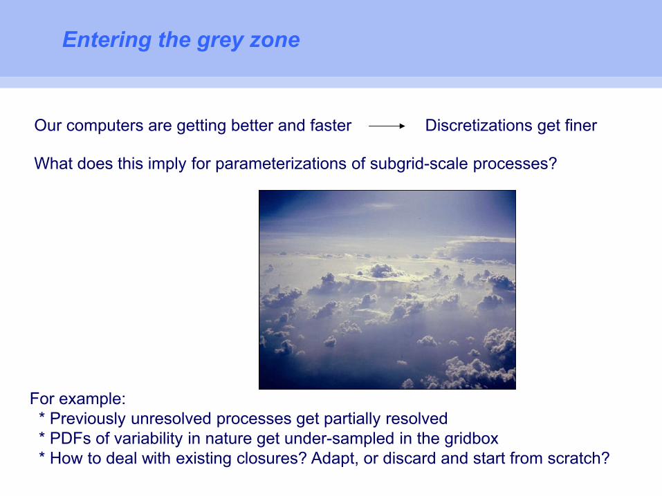
Entering the grey zone
Our computers are getting better and faster Discretizations get finer
What does this imply for parameterizations of subgrid-scale processes?
For example:* Previously unresolved processes get partially resolved* PDFs of variability in nature get under-sampled in the gridbox* How to deal with existing closures? Adapt, or discard and start from scratch?
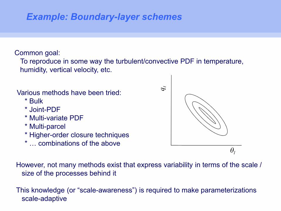
Example: Boundary-layer schemes
Common goal: To reproduce in some way the turbulent/convective PDF in temperature, humidity, vertical velocity, etc.
Various methods have been tried:* Bulk* Joint-PDF* Multi-variate PDF* Multi-parcel* Higher-order closure techniques* … combinations of the above
However, not many methods exist that express variability in terms of the scale / size of the processes behind it
This knowledge (or “scale-awareness”) is required to make parameterizations scale-adaptive
q t
l

Scale-adaptivity
What do we mean by that?
When a SGS parameterization is adaptive to the discretization-size of the 3D hostmodel in which it operates
Why do we care?
The question is what SGS parameterizations should represent
A finer horizontal discretization in a GCM means that smaller-scale processes become resolved
The work done by SGS parameterizations should adjust to this to avoid “double counting” and introduce stochastic effects
Low-res grid
High-res grid
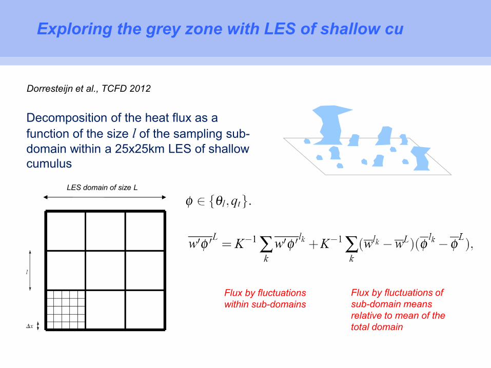
Exploring the grey zone with LES of shallow cu
Dorresteijn et al., TCFD 2012
LES domain of size L
Decomposition of the heat flux as a
function of the size l of the sampling sub-domain within a 25x25km LES of shallow cumulus
Flux by fluctuations within sub-domains
Flux by fluctuations of sub-domain means relative to mean of the total domain
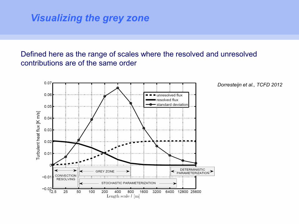
Visualizing the grey zone
Dorresteijn et al., TCFD 2012
Defined here as the range of scales where the resolved and unresolved contributions are of the same order
A summary of the problem
Current SGS parameterizations in GCMs are not scale-adaptive:
* Formulated in age (1970-present) when all types of convection were still totally unresolved
* Parameterizations do not “know” about the size of the process they are representing
The challenge: We have to stretch ourselves to make SGS models scale-adaptive, and thus “bridge the gap” between scales
However, the discretizations in operational GCMs are ever increasing:We are getting in the danger-zone or “grey zone”
Population dynamics
BxyAxt
x
DxyCyt
y
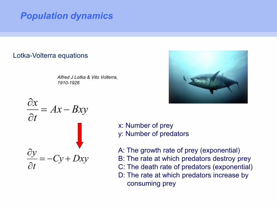
x: Number of preyy: Number of predators
A: The growth rate of prey (exponential)B: The rate at which predators destroy preyC: The death rate of predators (exponential)D: The rate at which predators increase by
consuming prey
Alfred J Lotka & Vito Volterra, 1910-1926
Lotka-Volterra equations

Time-dependent solutions
http://demonstrations.wolfram.com/PredatorPreyModel/
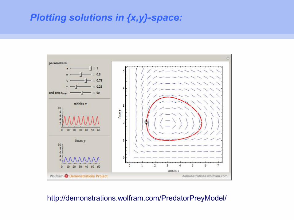
Plotting solutions in {x,y}-space:
http://demonstrations.wolfram.com/PredatorPreyModel/
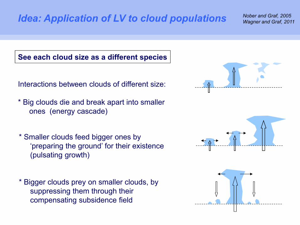
Idea: Application of LV to cloud populations
See each cloud size as a different species
Interactions between clouds of different size:
* Big clouds die and break apart into smaller ones (energy cascade)
* Smaller clouds feed bigger ones by ‘preparing the ground’ for their existence (pulsating growth)
* Bigger clouds prey on smaller clouds, by suppressing them through their compensating subsidence field
Nober and Graf, 2005Wagner and Graf, 2011
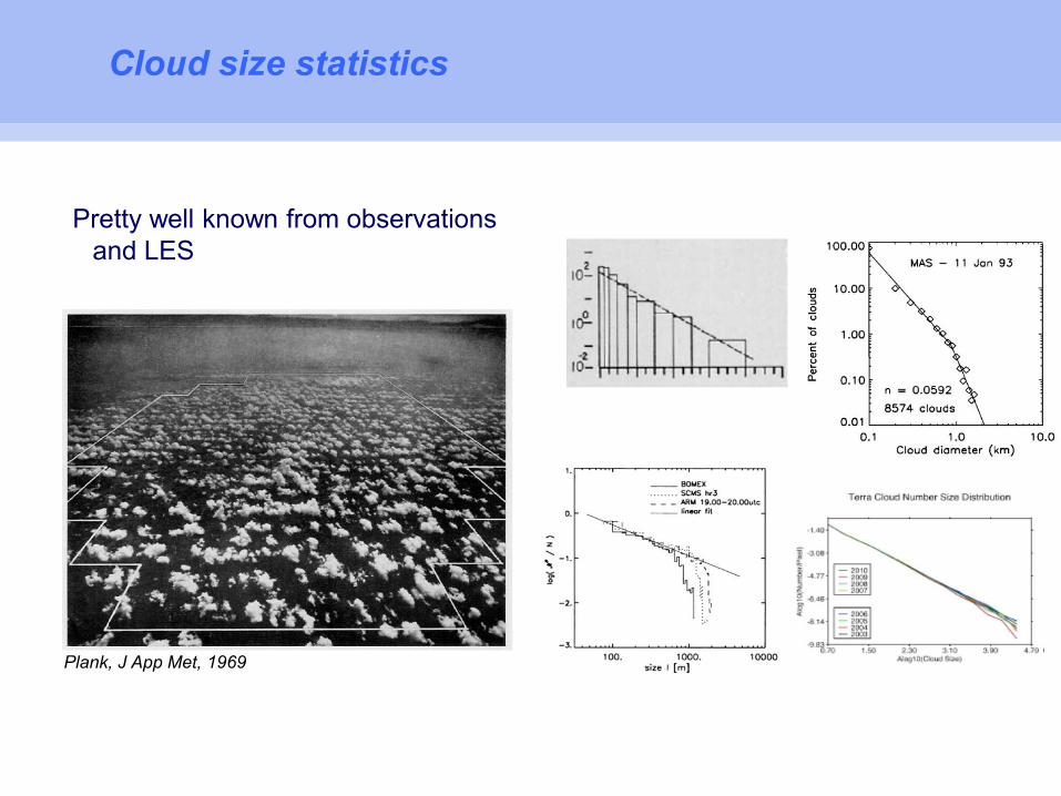
Cloud size statistics
Pretty well known from observations and LES
Plank, J App Met, 1969
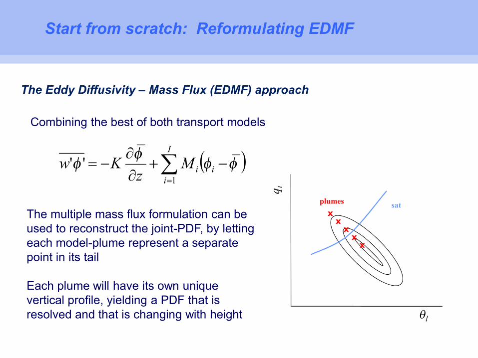
The Eddy Diffusivity – Mass Flux (EDMF) approach
Combining the best of both transport models
The multiple mass flux formulation can be used to reconstruct the joint-PDF, by letting each model-plume represent a separate point in its tail
Each plume will have its own unique vertical profile, yielding a PDF that is resolved and that is changing with height
I
iiiM
zKw
1
''
q t
l
xx
xx
satplumes
x
Start from scratch: Reformulating EDMF
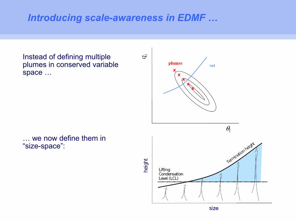
Introducing scale-awareness in EDMF …
… we now define them in “size-space”:
Instead of defining multiple plumes in conserved variable space …
Model formulation – Step I
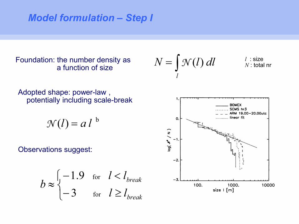
Foundation: the number density as a function of size
dllNl
)( N
b)( lal N
Adopted shape: power-law , potentially including scale-break
Observations suggest:
break
break
ll
llb
3
9.1
for
for
l : sizeN : total nr
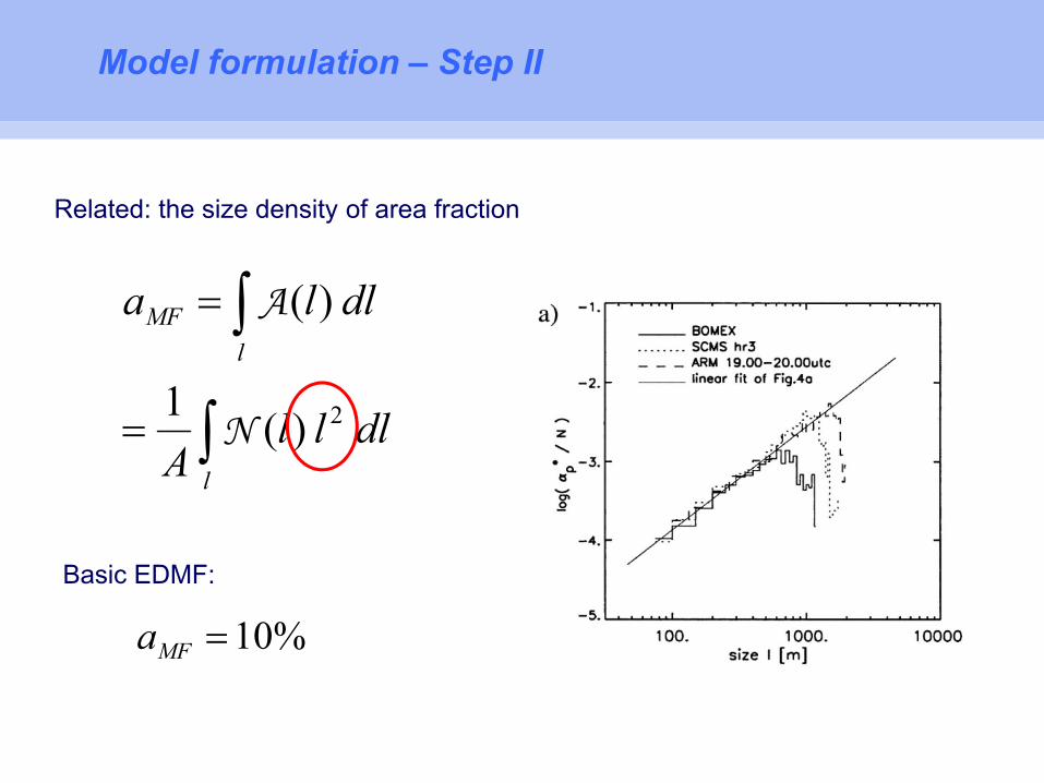
Model formulation – Step II
Related: the size density of area fraction
dlllA
dlla
l
l
MF
)(1
)(
2
N
A
Basic EDMF:
%10MFa
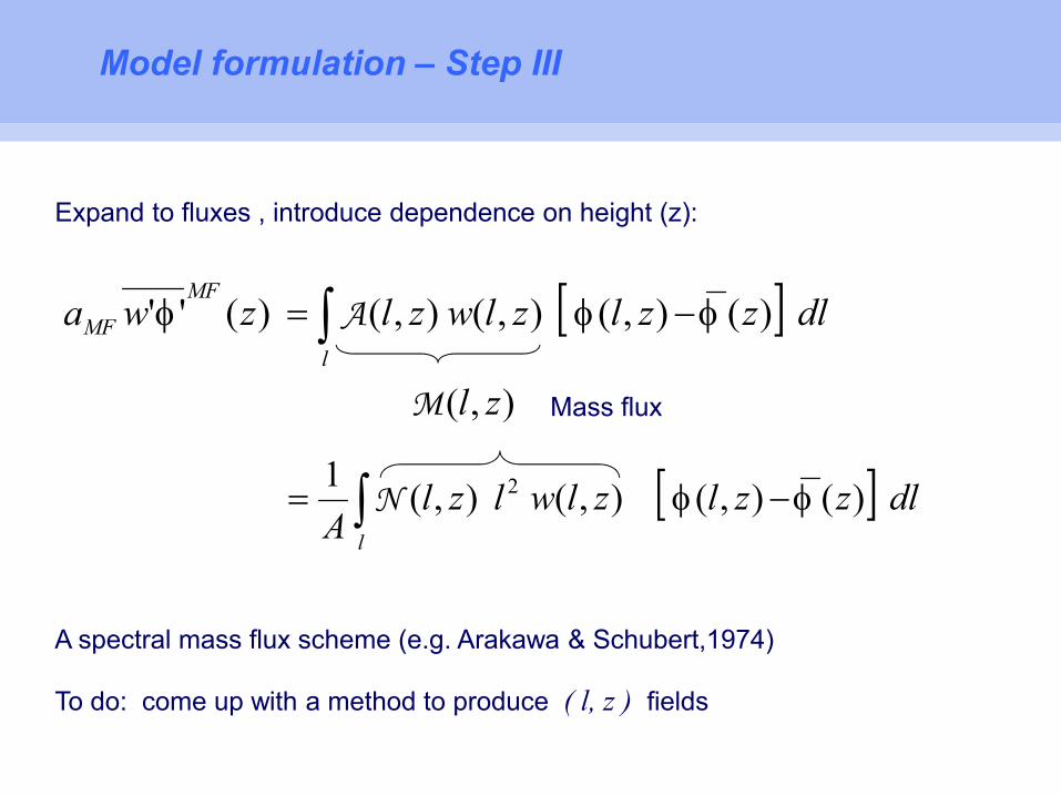
Model formulation – Step III
Expand to fluxes , introduce dependence on height (z):
dlzzlzlwzlzwal
MF
MF )(),( ),(),( )('' A
),( zlM
dlzzlzlwlzlA
l
)(),( ),( ),(1 2 N
To do: come up with a method to produce ( l, z ) fields
Mass flux
A spectral mass flux scheme (e.g. Arakawa & Schubert,1974)
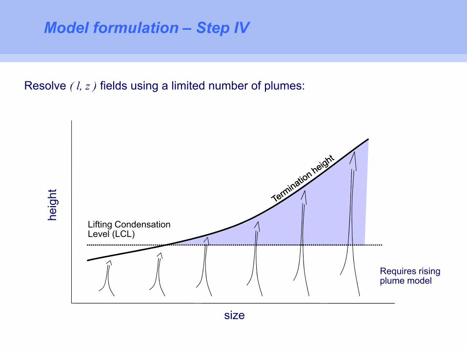
Model formulation – Step IV
Resolve ( l, z ) fields using a limited number of plumes:
size
heig
ht
Lifting Condensation Level (LCL)
Requires rising plume model
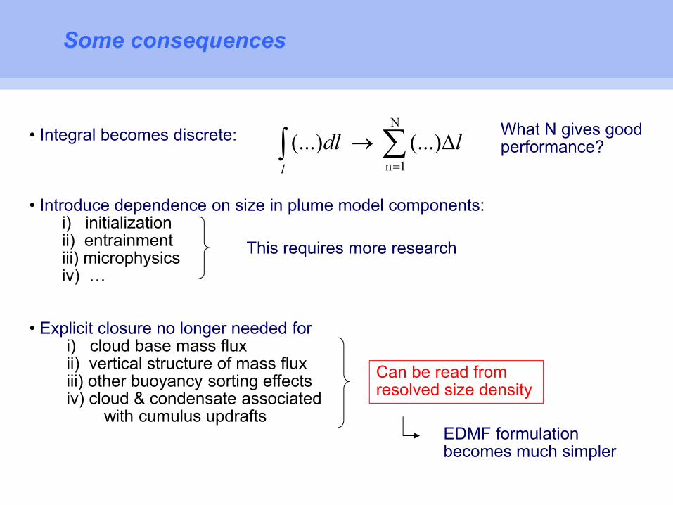
Some consequences
• Integral becomes discrete:
• Introduce dependence on size in plume model components:i) initializationii) entrainmentiii) microphysicsiv) …
• Explicit closure no longer needed fori) cloud base mass fluxii) vertical structure of mass fluxiii) other buoyancy sorting effects iv) cloud & condensate associated
with cumulus updrafts
N
1n
(...) (...) ldll
What N gives good performance?
This requires more research
Can be read from resolved size density
EDMF formulation becomes much simpler
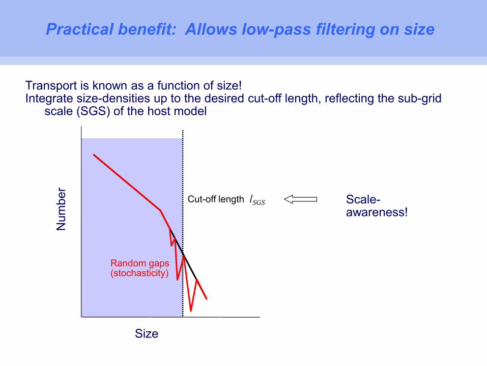
Transport is known as a function of size!Integrate size-densities up to the desired cut-off length, reflecting the sub-grid
scale (SGS) of the host model
Size
Num
ber
Cut-off length lSGS Scale-awareness!
Random gaps (stochasticity)
Practical benefit: Allows low-pass filtering on size
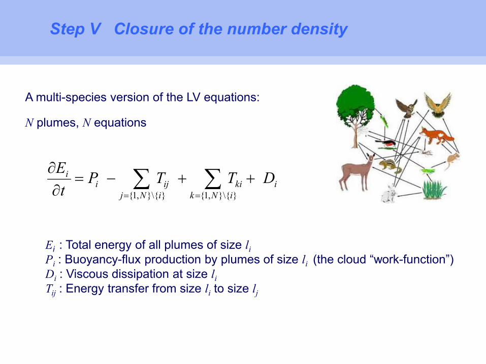
Step V Closure of the number density
A multi-species version of the LV equations:
N plumes, N equations
iiNk
kiiNj
ijii DTTP
t
E
}}\{,1{}}\{,1{
Ei : Total energy of all plumes of size li
Pi : Buoyancy-flux production by plumes of size li (the cloud “work-function”)Di : Viscous dissipation at size li
Tij : Energy transfer from size li to size lj
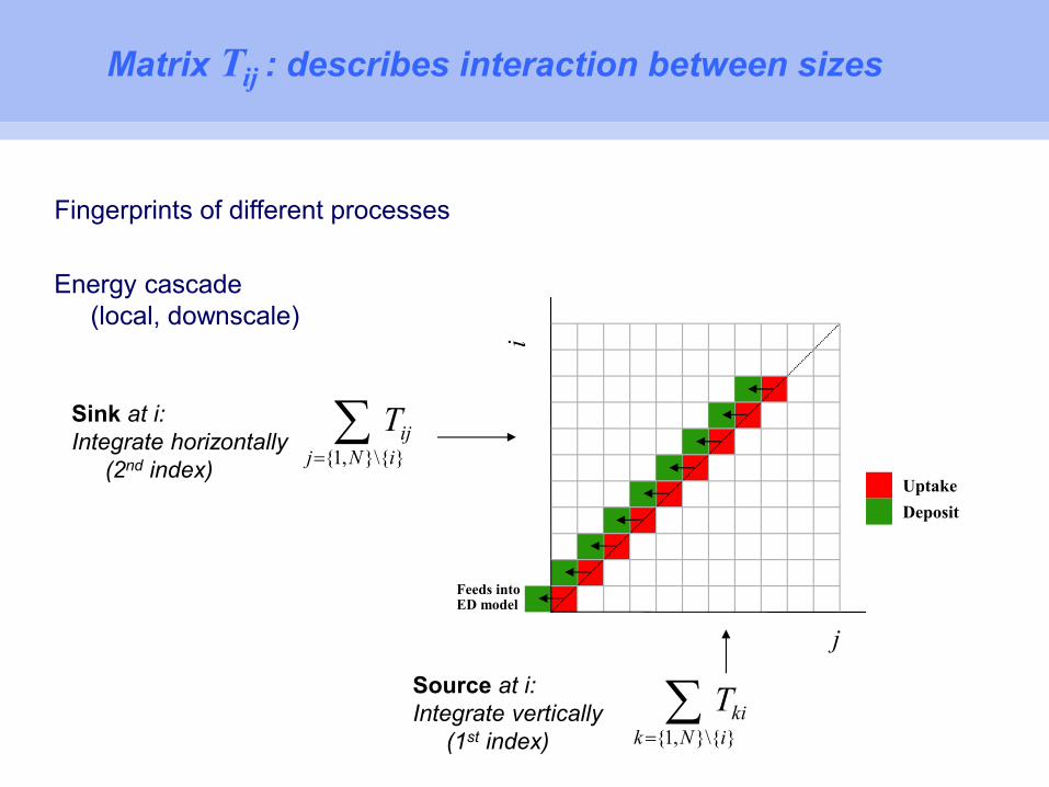
Matrix Tij : describes interaction between sizes
Fingerprints of different processes
Energy cascade (local, downscale)
i
j
Feeds into ED model
Uptake
Deposit
}}\{,1{
iNjijT
}}\{,1{ iNk
kiT
Sink at i: Integrate horizontally
(2nd index)
Source at i:Integrate vertically
(1st index)
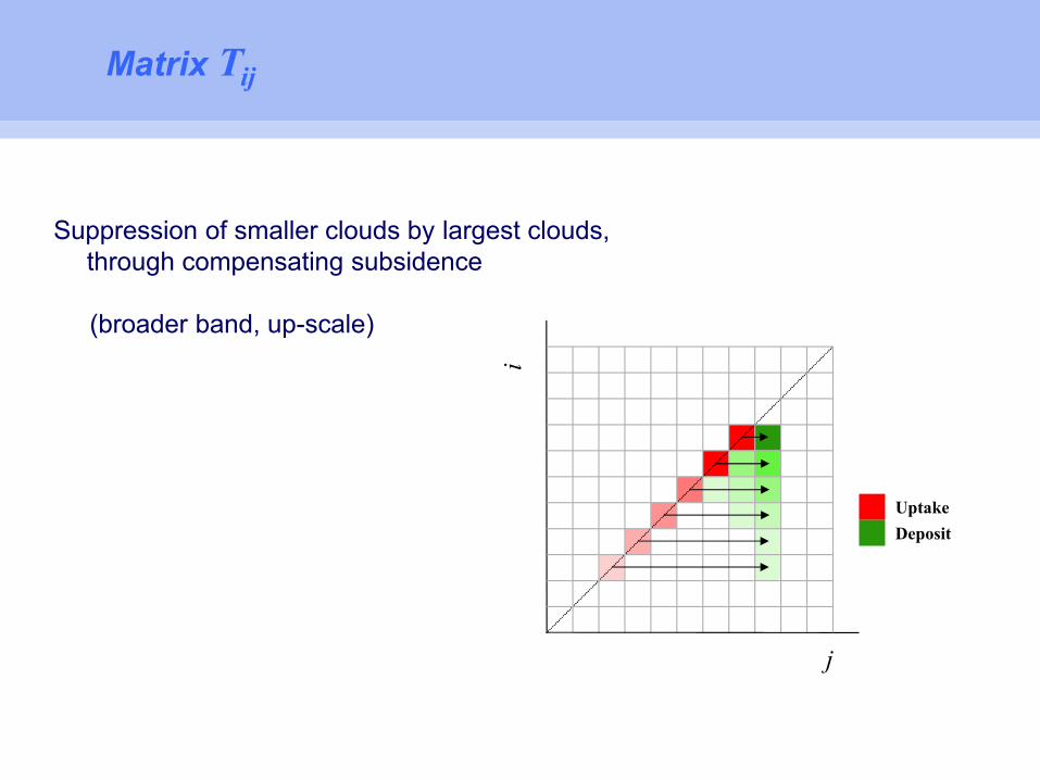
Matrix Tij
Suppression of smaller clouds by largest clouds, through compensating subsidence
(broader band, up-scale)
i
j
Uptake
Deposit
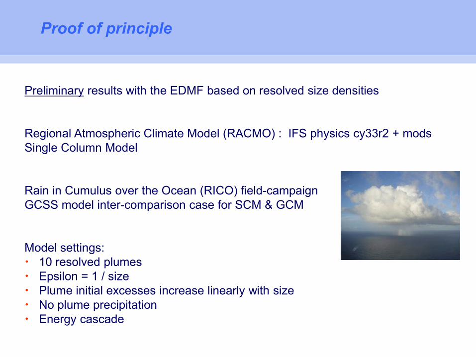
Preliminary results with the EDMF based on resolved size densities
Regional Atmospheric Climate Model (RACMO) : IFS physics cy33r2 + modsSingle Column Model
Rain in Cumulus over the Ocean (RICO) field-campaignGCSS model inter-comparison case for SCM & GCM
Model settings:• 10 resolved plumes• Epsilon = 1 / size• Plume initial excesses increase linearly with size• No plume precipitation• Energy cascade
Proof of principle
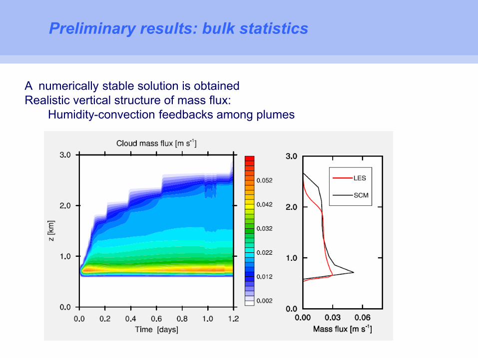
Preliminary results: bulk statistics
A numerically stable solution is obtainedRealistic vertical structure of mass flux:
Humidity-convection feedbacks among plumes
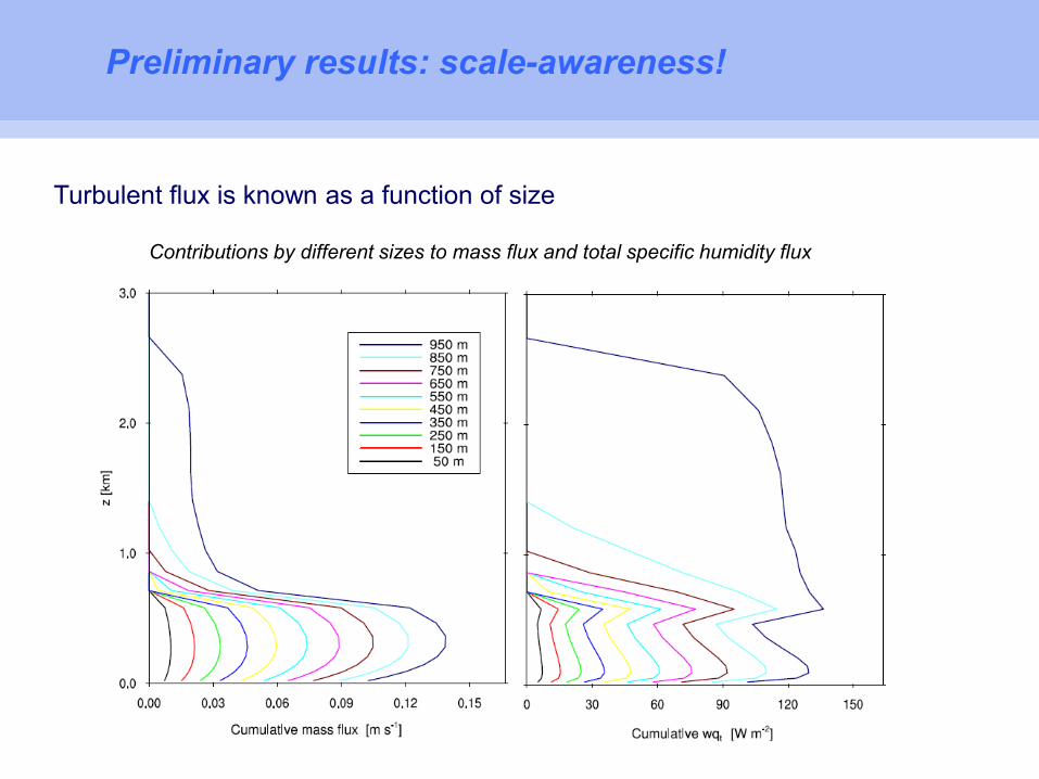
Preliminary results: scale-awareness!
Turbulent flux is known as a function of size
Contributions by different sizes to mass flux and total specific humidity flux
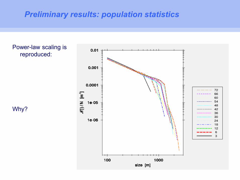
Preliminary results: population statistics
Power-law scaling is reproduced:
Why?
Power law scaling
* Energy is transferred from a larger size to a smaller size
Why a scale break?
* Latent heat release by the larger plumes significantly boosts their kinetic energy
* As a result, fewer big clouds are necessary to compose a given amount of energy
* But individual plumes of smaller size carry less energy than big ones
* As a result, the same energy can be shared by more plumes, yielding a higher number
Outlook
Conceptual models describing population dynamics can be applied to make SGS parameterizations scale-aware and scale-adaptive
The development of such models for operational GCMs is in progress, but most implementations are still in testing-phase
Observations and high-resolution modelling results are needed to properly constrain this new type of scale-aware parameterization
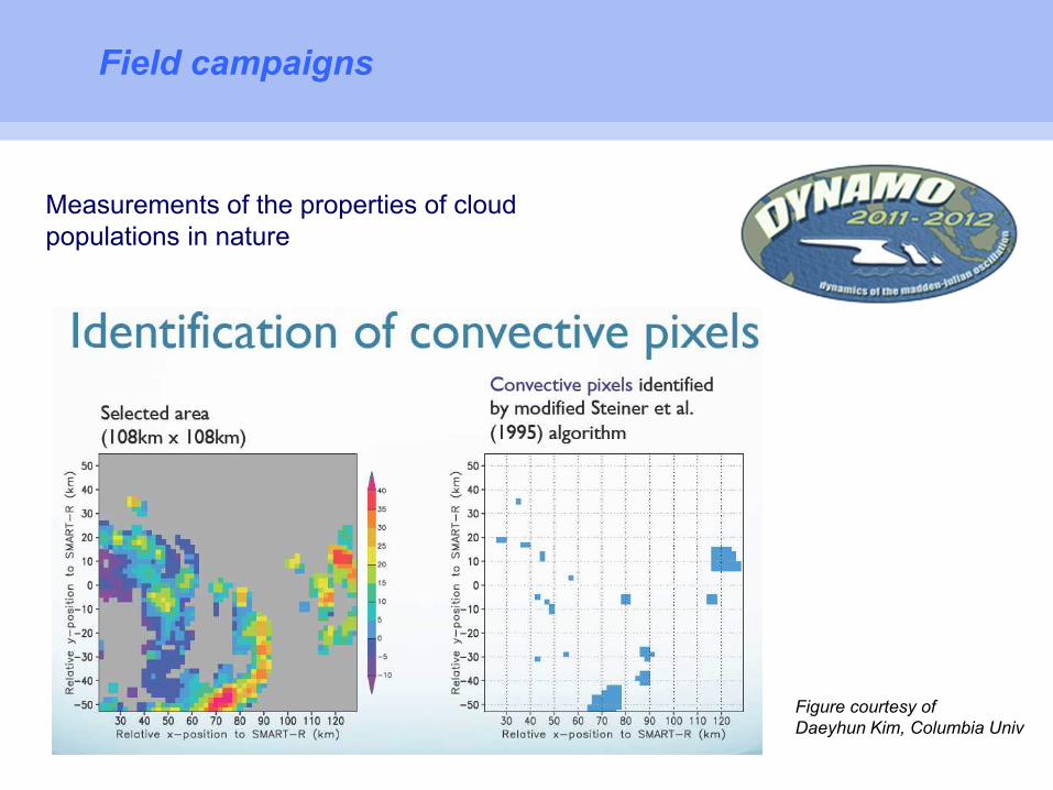
Field campaigns
Measurements of the properties of cloud populations in nature
Figure courtesy of Daeyhun Kim, Columbia Univ
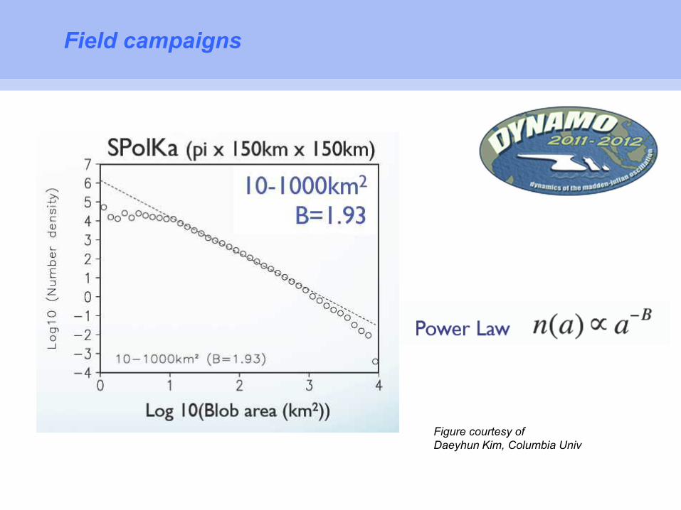
Field campaigns
Figure courtesy of Daeyhun Kim, Columbia Univ
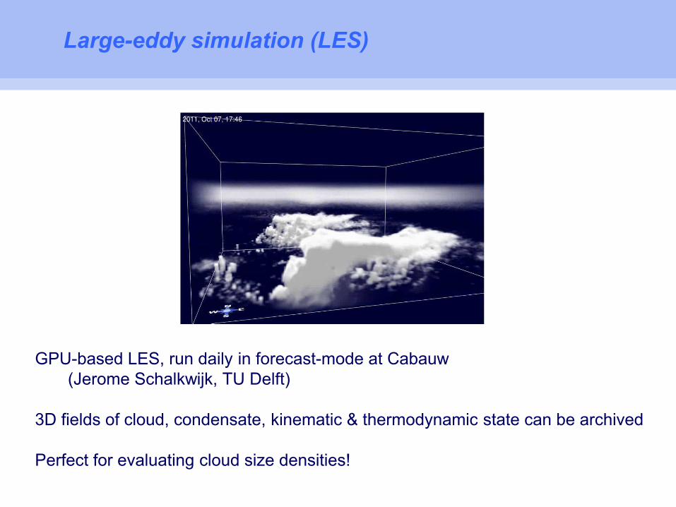
Large-eddy simulation (LES)
GPU-based LES, run daily in forecast-mode at Cabauw(Jerome Schalkwijk, TU Delft)
3D fields of cloud, condensate, kinematic & thermodynamic state can be archived
Perfect for evaluating cloud size densities!