Embed Size (px)
Citation preview
DePaul University DePaul University
Via Sapientiae Via Sapientiae
College of Computing and Digital Media Dissertations College of Computing and Digital Media
Fall 11-2013
Towards Automated Network Configuration Management Towards Automated Network Configuration Management
Khalid Elmansor DePaul University, [email protected]
Follow this and additional works at: https://via.library.depaul.edu/cdm_etd
Part of the OS and Networks Commons
Recommended Citation Recommended Citation Elmansor, Khalid, "Towards Automated Network Configuration Management" (2013). College of Computing and Digital Media Dissertations. 5. https://via.library.depaul.edu/cdm_etd/5
This Dissertation is brought to you for free and open access by the College of Computing and Digital Media at Via Sapientiae. It has been accepted for inclusion in College of Computing and Digital Media Dissertations by an authorized administrator of Via Sapientiae. For more information, please contact [email protected].
DePaul University
College of Computing and Digital Media
School of Computing
Towards Automated Network
Configuration Management
by
Khalid Elmansor
A dissertation Submitted to
the college of Computing and Digital Media
in partial fulfillment of the requirements of the degree of
Doctor of Philosophy
Supervisor: James Yu
Chicago, IL, 2013


DePaul University
College of Computing and Digital Media
School of Computing
Abstract
Towards Automated Network Configuration Management
Khalid Elmansor
Modern networks are designed to satisfy a wide variety of competing goals related to network
operation requirements such as reachability, security, performance, reliability and availability.
These high level goals are realized through a complex chain of low level configuration commands
performed on network devices.
As networks become larger, more complex and more heterogeneous, human errors become
the most significant threat to network operation and the main cause of network outage. In
addition, the gap between high-level requirements and low-level configuration data is continu-
ously increasing and difficult to close. Although many solutions have been introduced to reduce
the complexity of configuration management, network changes, in most cases, are still manually
performed via low–level command line interfaces (CLIs). The Internet Engineering Task Force
(IETF) has introduced NETwork CONFiguration (NETCONF) protocol along with its associ-
ated data–modeling language, YANG, that significantly reduce network configuration complexity.
However, NETCONF is limited to the interaction between managers and agents, and it has weak
support for compliance to high-level management functionalities.
We design and develop a network configuration management system called AutoConf that
addresses the aforementioned problems. AutoConf is a distributed system that manages, vali-
dates, and automates the configuration of IP networks. We propose a new framework to aug-
ment NETCONF/YANG framework. This framework includes a Configuration Semantic Model

(CSM), which provides a formal representation of domain knowledge needed to deploy a suc-
cessful management system. Along with CSM, we develop a domain–specific language called
Structured Configuration language to specify configuration tasks as well as high–level require-
ments. CSM/SCL together with NETCONF/YANG makes a powerful management system that
supports network–wide configuration. AutoConf supports two levels of verifications: consistency
verification and behavioral verification. We apply a set of logical formalizations to verifying the
consistency and dependency of configuration parameters. In behavioral verification, we present
a set of formal models and algorithms based on Binary Decision Diagram (BDD) to capture the
behaviors of forwarding control lists that are deployed in firewalls, routers, and NAT devices. We
also adopt an enhanced version of Dyna-Q algorithm to support dynamic adaptation of network
configuration in response to changes occurred during network operation. This adaptation ap-
proach maintains a coherent relationship between high level requirements and low level device
configuration.
We evaluate AutoConf by running several configuration scenarios such as interface configu-
ration, RIP configuration, OSPF configuration and MPLS configuration. We also evaluate Au-
toConf by running several simulation models to demonstrate the effectiveness and the scalability
of handling large-scale networks.

This dissertation is lovingly dedicated to my family


Acknowledgements
First and foremost, I would like to thank the Almighty Allah, the compassionate, the mer-
ciful, for his countless blessing.
The success of this dissertation is attributed to the extensive guidance and assistance from
my supervisor, Prof. James Yu. I would like to express my grateful gratitude and sincere
appreciation to him for his support, supervision, encouragement and kindness throughout
this study. I simply cannot imagine how things would have proceeded without his help and
his extreme patience.
I am deeply indebted to Prof. Yongning Tang for his continuous support, friendship and
encouragement. I highly appreciate all his efforts, time and ideas to make my Ph.D. work
successful and complete.
In addition, I would like to thank the College of Computing and Digital Media (CDM)
at DePaul University for supporting this research work. I specially want to thank Prof.
Anthony Chung and Prof. Gregory Brewster for their valuable comments and suggestions
in reviewing my research work.
I also acknowledge my many colleagues and friends as I had a pleasant, enjoyable and
fruitful company with them.
Finally, I wish to express my gratitude to my family members for being patient with me
and offering words of encouragement to spur my spirit at moments of depression.
vii


Contents
Contents i
List of Figures vii
List of Tables ix
1 Introduction 1
1.1 Motivation . . . . . . . . . . . . . . . . . . . . . . . . . . . . . . . . . . . . . 2
1.2 Problem Statement . . . . . . . . . . . . . . . . . . . . . . . . . . . . . . . . 6
1.3 Scope . . . . . . . . . . . . . . . . . . . . . . . . . . . . . . . . . . . . . . . 7
1.4 Goals and Contributions . . . . . . . . . . . . . . . . . . . . . . . . . . . . . 7
1.5 Organization . . . . . . . . . . . . . . . . . . . . . . . . . . . . . . . . . . . 8
2 Background and Literature Review 11
2.1 Binary Decision Diagram . . . . . . . . . . . . . . . . . . . . . . . . . . . . . 11
2.2 Reinforcement Learning . . . . . . . . . . . . . . . . . . . . . . . . . . . . . 15
2.3 Network Management Architectures . . . . . . . . . . . . . . . . . . . . . . . 18
2.3.1 OSI Management . . . . . . . . . . . . . . . . . . . . . . . . . . . . . 19
2.3.2 TMN management . . . . . . . . . . . . . . . . . . . . . . . . . . . . 25
2.3.3 Internet Management . . . . . . . . . . . . . . . . . . . . . . . . . . . 32
2.3.4 Discussion and Critique . . . . . . . . . . . . . . . . . . . . . . . . . 37
i

ii CONTENTS
2.4 Network Management Protocols . . . . . . . . . . . . . . . . . . . . . . . . . 38
2.4.1 Common Management Information Protocol . . . . . . . . . . . . . . 38
2.4.2 Simple Network Management Protocol . . . . . . . . . . . . . . . . . 40
2.4.3 Network Configuration Protocol . . . . . . . . . . . . . . . . . . . . . 42
2.4.4 Discussion and Critique . . . . . . . . . . . . . . . . . . . . . . . . . 46
2.5 Current approaches to network Configuration . . . . . . . . . . . . . . . . . 48
2.5.1 Manual configuration . . . . . . . . . . . . . . . . . . . . . . . . . . . 48
2.5.2 Script-based and template-based configuration . . . . . . . . . . . . . 49
2.5.3 Vendor-neutral Configuration . . . . . . . . . . . . . . . . . . . . . . 50
2.5.4 Declarative-based Configuration . . . . . . . . . . . . . . . . . . . . . 51
2.5.5 Policy-based approach . . . . . . . . . . . . . . . . . . . . . . . . . . 53
2.5.6 Separating Data and Control planes approaches . . . . . . . . . . . . 54
2.5.7 Discussion and Critique . . . . . . . . . . . . . . . . . . . . . . . . . 55
2.6 Configuration Verification Approaches . . . . . . . . . . . . . . . . . . . . . 57
2.7 Summary . . . . . . . . . . . . . . . . . . . . . . . . . . . . . . . . . . . . . 58
3 Configuration Semantic Model 59
3.1 Overview . . . . . . . . . . . . . . . . . . . . . . . . . . . . . . . . . . . . . . 59
3.2 The framework . . . . . . . . . . . . . . . . . . . . . . . . . . . . . . . . . . 61
3.3 Configuration Semantic Model Concepts . . . . . . . . . . . . . . . . . . . . 63
3.3.1 Topology Specification . . . . . . . . . . . . . . . . . . . . . . . . . . 64
3.3.2 Configuration Specification . . . . . . . . . . . . . . . . . . . . . . . . 66
3.3.3 State and Policy Specification . . . . . . . . . . . . . . . . . . . . . . 67
3.3.4 Overall Organization . . . . . . . . . . . . . . . . . . . . . . . . . . . 67
3.4 Structured Configuration Language . . . . . . . . . . . . . . . . . . . . . . . 67
3.4.1 Improved Configuration Management . . . . . . . . . . . . . . . . . . 69
3.5 Summary . . . . . . . . . . . . . . . . . . . . . . . . . . . . . . . . . . . . . 71

CONTENTS iii
4 Configuration Verification 73
4.1 Overview . . . . . . . . . . . . . . . . . . . . . . . . . . . . . . . . . . . . . . 73
4.2 Network Verification Levels . . . . . . . . . . . . . . . . . . . . . . . . . . . 74
4.3 Consistency Verification . . . . . . . . . . . . . . . . . . . . . . . . . . . . . 76
4.3.1 Data–level Verification . . . . . . . . . . . . . . . . . . . . . . . . . . 76
4.3.2 Device and Service-level verification . . . . . . . . . . . . . . . . . . . 77
4.3.3 Link-level verification . . . . . . . . . . . . . . . . . . . . . . . . . . . 79
4.3.4 SCL Language Related to Consistency Verification . . . . . . . . . . 79
4.4 Behavioral Verification . . . . . . . . . . . . . . . . . . . . . . . . . . . . . . 82
4.4.1 Formal Representation of Forwarding Control List . . . . . . . . . . . 82
4.4.2 Link-level Behavior . . . . . . . . . . . . . . . . . . . . . . . . . . . . 94
4.4.3 Network-level Behavior . . . . . . . . . . . . . . . . . . . . . . . . . . 96
4.4.4 Impact of Configuration Change . . . . . . . . . . . . . . . . . . . . . 98
4.4.5 SCL Language Related to Behavioral Verification . . . . . . . . . . . 99
4.5 Summary . . . . . . . . . . . . . . . . . . . . . . . . . . . . . . . . . . . . . 101
5 Configuration Automation 103
5.1 Overview . . . . . . . . . . . . . . . . . . . . . . . . . . . . . . . . . . . . . . 103
5.2 Policy Structure . . . . . . . . . . . . . . . . . . . . . . . . . . . . . . . . . . 106
5.2.1 Policy Condition . . . . . . . . . . . . . . . . . . . . . . . . . . . . . 106
5.2.2 Policy Action . . . . . . . . . . . . . . . . . . . . . . . . . . . . . . . 108
5.2.3 Policy Type . . . . . . . . . . . . . . . . . . . . . . . . . . . . . . . . 109
5.3 Automation Model . . . . . . . . . . . . . . . . . . . . . . . . . . . . . . . . 110
5.3.1 Policy Representation . . . . . . . . . . . . . . . . . . . . . . . . . . 111
5.3.2 Policy Manipulations . . . . . . . . . . . . . . . . . . . . . . . . . . . 114
5.3.3 System State Representation . . . . . . . . . . . . . . . . . . . . . . . 115
5.3.4 Action Selection . . . . . . . . . . . . . . . . . . . . . . . . . . . . . . 117
5.3.5 The Reward Function . . . . . . . . . . . . . . . . . . . . . . . . . . . 118
iv CONTENTS
5.4 Summary . . . . . . . . . . . . . . . . . . . . . . . . . . . . . . . . . . . . . 122
6 Implementation 125
6.1 Erlang Language . . . . . . . . . . . . . . . . . . . . . . . . . . . . . . . . . 125
6.2 Overall Architecture . . . . . . . . . . . . . . . . . . . . . . . . . . . . . . . 127
6.3 SCL Grammar . . . . . . . . . . . . . . . . . . . . . . . . . . . . . . . . . . 130
6.4 Configuration Change Implementation . . . . . . . . . . . . . . . . . . . . . 130
6.5 Configuration Verification Implementation . . . . . . . . . . . . . . . . . . . 132
6.6 Configuration Automation Implementation . . . . . . . . . . . . . . . . . . . 132
6.7 Summary . . . . . . . . . . . . . . . . . . . . . . . . . . . . . . . . . . . . . 133
7 Experimental and Evaluation Results 135
7.1 Experimental Setup . . . . . . . . . . . . . . . . . . . . . . . . . . . . . . . . 135
7.2 Basic Configuration Scenarios . . . . . . . . . . . . . . . . . . . . . . . . . . 139
7.2.1 Topology specification . . . . . . . . . . . . . . . . . . . . . . . . . . 140
7.2.2 Interface configuration . . . . . . . . . . . . . . . . . . . . . . . . . . 141
7.2.3 RIP configuration . . . . . . . . . . . . . . . . . . . . . . . . . . . . . 145
7.2.4 OSPF configuration . . . . . . . . . . . . . . . . . . . . . . . . . . . . 147
7.2.5 MPLS VPN Configuration . . . . . . . . . . . . . . . . . . . . . . . . 149
7.2.6 Automating interface configuration . . . . . . . . . . . . . . . . . . . 152
7.2.7 Automating Filtering policy . . . . . . . . . . . . . . . . . . . . . . . 153
7.3 Evaluating Verification System using Simulation . . . . . . . . . . . . . . . . 154
7.3.1 Topology and FCL Generator . . . . . . . . . . . . . . . . . . . . . . 155
7.3.2 Evaluating BDD Construction . . . . . . . . . . . . . . . . . . . . . . 156
7.3.3 End–to–End Verification Analysis . . . . . . . . . . . . . . . . . . . . 158
7.4 Evaluating AutoConf using Simulation . . . . . . . . . . . . . . . . . . . . . 160
7.4.1 Requirements and State Generator . . . . . . . . . . . . . . . . . . . 160
7.4.2 Evaluating BDD Construction . . . . . . . . . . . . . . . . . . . . . . 161
CONTENTS v
7.5 Summary . . . . . . . . . . . . . . . . . . . . . . . . . . . . . . . . . . . . . 164
8 Conclusion 165
8.1 Limitations . . . . . . . . . . . . . . . . . . . . . . . . . . . . . . . . . . . . 166
8.2 Future work . . . . . . . . . . . . . . . . . . . . . . . . . . . . . . . . . . . . 167
Bibliography 169
A YANG language 183
B Structured Configuration Language 189
B.1 Language Primitives . . . . . . . . . . . . . . . . . . . . . . . . . . . . . . . 189
B.2 SCL statements . . . . . . . . . . . . . . . . . . . . . . . . . . . . . . . . . . 189
B.2.1 Schema statement . . . . . . . . . . . . . . . . . . . . . . . . . . . . . 190
B.2.2 Insert statement . . . . . . . . . . . . . . . . . . . . . . . . . . . . . . 190
B.2.3 Sequence generator statement . . . . . . . . . . . . . . . . . . . . . . 191
B.2.4 Manage statement . . . . . . . . . . . . . . . . . . . . . . . . . . . . 191
List of Symbols and Abbreviations 193

List of Figures
1.1 Network Operator errors are the major cause of network downtime . . . . . . . 3
1.2 IPv6 Security Concerns . . . . . . . . . . . . . . . . . . . . . . . . . . . . . . . . 4
2.1 The real and formal worlds illustrated by two circles. . . . . . . . . . . . . . . . 12
2.2 Decision diagram for x1 ∧ x2 ∨ x3 . . . . . . . . . . . . . . . . . . . . . . . . . . 13
2.3 OSI abstraction for managed objects . . . . . . . . . . . . . . . . . . . . . . . . 21
2.4 Relationships between management functions and user requirements . . . . . . . 22
2.5 Manager-agent Interactions . . . . . . . . . . . . . . . . . . . . . . . . . . . . . 24
2.6 TMN network management concept . . . . . . . . . . . . . . . . . . . . . . . . . 26
2.7 MAFs interactions . . . . . . . . . . . . . . . . . . . . . . . . . . . . . . . . . . 28
2.8 TMN Functional Layering . . . . . . . . . . . . . . . . . . . . . . . . . . . . . . 31
2.9 SMI object tree . . . . . . . . . . . . . . . . . . . . . . . . . . . . . . . . . . . . 34
2.10 SNMPv3 Entity . . . . . . . . . . . . . . . . . . . . . . . . . . . . . . . . . . . . 36
2.11 The flow model of CMIP PDUs . . . . . . . . . . . . . . . . . . . . . . . . . . . 40
2.12 SNMP message format . . . . . . . . . . . . . . . . . . . . . . . . . . . . . . . . 42
2.13 NETCONF’s conceptual layers . . . . . . . . . . . . . . . . . . . . . . . . . . . 43
3.1 Life cycle of a networked device . . . . . . . . . . . . . . . . . . . . . . . . . . . 60
3.2 AutoConf management system . . . . . . . . . . . . . . . . . . . . . . . . . . . . 61
3.3 AutoConf framework . . . . . . . . . . . . . . . . . . . . . . . . . . . . . . . . . 63
vii
viii LIST OF FIGURES
3.4 The hierarchical structure of Configuration Specification . . . . . . . . . . . . . 68
3.5 A network with a set of edge and core routers . . . . . . . . . . . . . . . . . . . 70
4.1 XSLT transforms XML documents to another XML documents . . . . . . . . . 78
4.2 FCL policy with m different decisions partitioning flow Π into m sub–flows. . . 83
4.3 A network with three subnetworks connected via three routers . . . . . . . . . . 90
4.4 The graph model of a simple network . . . . . . . . . . . . . . . . . . . . . . . . 97
5.1 Policy–based management . . . . . . . . . . . . . . . . . . . . . . . . . . . . . . 105
5.2 High-level policy rules are translated to low-level requirements . . . . . . . . . . 111
5.3 The effect of taking an action at state S after which the system will be in state S ′120
5.4 A sample of state–transition diagram . . . . . . . . . . . . . . . . . . . . . . . . 121
6.1 AutoConf management architecture . . . . . . . . . . . . . . . . . . . . . . . . . 128
6.2 AutoConf Application running in Erlang system . . . . . . . . . . . . . . . . . . 129
7.1 Experimatal Network setup . . . . . . . . . . . . . . . . . . . . . . . . . . . . . 139
7.2 Interface configuration as generated by AutoConf Executer . . . . . . . . . . . . 142
7.3 OSPF links setup . . . . . . . . . . . . . . . . . . . . . . . . . . . . . . . . . . . 149
7.4 Customer wants to link its two Sites (Site1 and Site2) . . . . . . . . . . . . . . . 150
7.5 Comparing between Equation 4.7 and Equation 4.4 in terms of memory complexity157
7.6 BDD construction time for firewall policies less than 10 thousands . . . . . . . . 158
7.7 BDD construction time for huge set of firewall policies . . . . . . . . . . . . . . 158
7.8 Space complexity for BDD construction . . . . . . . . . . . . . . . . . . . . . . . 159
7.9 AutoConf performance with respect to memory complexity . . . . . . . . . . . . 159
7.10 AutoConf performance with respect to time complexity . . . . . . . . . . . . . . 159
7.11 The impact of requirement’s set size to the BDD construction time . . . . . . . 162
7.12 The impact of network size to the BDD construction time . . . . . . . . . . . . 163
7.13 The time required to construct network states’ BDD . . . . . . . . . . . . . . . 164
List of Tables
2.1 Sample of filtering policy . . . . . . . . . . . . . . . . . . . . . . . . . . . . . . . 12
2.2 Boolean variables distribution over constraint fields . . . . . . . . . . . . . . . . 14
2.3 Systems management functions . . . . . . . . . . . . . . . . . . . . . . . . . . . 23
2.4 Relation between function blocks expressed as reference points . . . . . . . . . . 29
2.5 CMIP operations and their equivalent CMIS services . . . . . . . . . . . . . . . 39
4.1 Quantifier values . . . . . . . . . . . . . . . . . . . . . . . . . . . . . . . . . . . 77
4.2 Set operations and their equivalent BDD operations . . . . . . . . . . . . . . . . 85
5.1 Expressing a relational operator as a set of values . . . . . . . . . . . . . . . . . 108
5.2 Optimal policy with positive rewards in each state . . . . . . . . . . . . . . . . . 121
5.3 Optimal policy with negative rewards, in each state . . . . . . . . . . . . . . . . 122
7.1 IP Subnet Plan . . . . . . . . . . . . . . . . . . . . . . . . . . . . . . . . . . . . 141
7.2 Time Performance as reported in previous work . . . . . . . . . . . . . . . . . . 157
7.3 Experimental Results for Analyzing FCL rules . . . . . . . . . . . . . . . . . . . 158
7.4 Metric–spec Categories . . . . . . . . . . . . . . . . . . . . . . . . . . . . . . . . 162
ix

Chapter 1
Introduction
The aim of network management is to provide to network-based services and applications
a networked system with the desired level of quality and availability, and to provide a
mechanism for a rapid, flexible deployment of networked resources. Hegering [37] describes
management of networked systems as a collection of all measures necessary to ensure the ef-
fective and efficient operation of a system and its resources pursuant to corporate goals. The
Telecommunication Standardization Sector of the International Telecommunication Union
(ITU-T) defines management as a set of capabilities to allow for the exchange and process-
ing of management information to assist Public Telecommunication Operators (PTOs) in
conducting their business efficiently [48]. Therefore, network management is any activity
(planning, configuration, monitoring, etc) that ensures the proper operation of a network
that satisfies certain high–level requirements such as business, performance, security, con-
nectivity and availability.
The International Organization for Standardizations (ISO) has divided management ac-
tivities into five functional areas: Fault, Configuration, Accounting, Performance and Secu-
rity [44]. Fault management concerns on monitoring devices activities, detecting faults, and
performing root-cause analysis to isolate and correct the abnormal conditions. Configura-
tion management concerns with the ability to access configuration data in order to add new
1
2 CHAPTER 1. INTRODUCTION
configuration, delete an existing configuration, or update a configuration data. Account-
ing management concerns on billing and accounting issues related to the use of network
resources. Performance management concerns on assessing and evaluating network perfor-
mance. Security management concerns with the ability to provide security assurance and
protection.
Unlike other functional areas of network management, where read-only operations are
performed on network devices to collect operational information, configuration management
makes adjustment to the configuration data in order to enable (or disable) network services.
In fact, network cannot operate without initially be configured; if network devices are not
properly configured, there is no network! Furthermore, all other management functions rely
on configuration management to accomplish the desired output. For examples, fault man-
agement requires reconfiguration to fix the problems, performance management requires
reconfiguration to optimize the network operation, and security management requires re-
configuration to resolve any security violation. Consequently, configuration management is
considered the most important management function among other functional areas.
The remaining of this chapter is organized as follows. We first discuss the motivation
of our dissertation. Then, we state the problem statement of our research work. Next, we
describe the scope of this dissertation and limitations. The following section then lists our
contributions. We conclude this chapter with a brief summary on how this dissertation is
organized.
1.1 Motivation
Network Configuration management is a complicated task. This is because of the immense
complexity and diversity of the underlying network devices such as switches, routers, fire-
walls, IPSECs, VPN access points, etc. Moreover, many enterprises and service providers are
supporting different services and configurations that put network administrators in a very
1.1. MOTIVATION 3
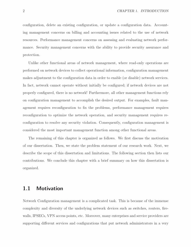
Source: The Yankee Group 2002 Network Downtime Survey
Figure 1.1: Network Operator errors are the major cause of network downtime
difficult task. The complexity of configuration management is not only due to the existence
of a huge set of configuration parameters, but also the existence of implicit dependencies
between these parameters. Network administrators are continuously requested to conduct
provisioning or performance tuning. However, changing one configuration parameter may
bring a complex chain of changes that network administrators must anticipate it. As net-
works grow larger, configuring and debugging these networks become too complicated. The
complication is getting worse when the network is composed of multi-vendor network de-
vices. Consequently, network administrators, who rely on CLIs, need to remember a myriad
of commands, protocols, and device architectures. This certainly causes a critical prob-
lem for market demands which require quick and accurate deployment of new services to
maintain the revenue.
All these complications increase the chances of faulty configurations. The study in [70]
revealed that network administrator errors are the largest cause of network failure (around
61%) as shown in Figure 1.1. Analysis from IT experts states that human errors are re-
sponsible for 50 to 80 percent of network device outages [93]. In 2010, Arbor Networks [2]
has published a security survey report. The participants of the survey were from Tier 1,
Tier 2 and other IP network operators. Even though the report was focusing on security
issues, 61% of survey participants indicated that misconfiguration is the most significant
4 CHAPTER 1. INTRODUCTION
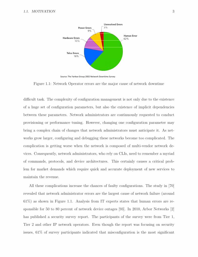
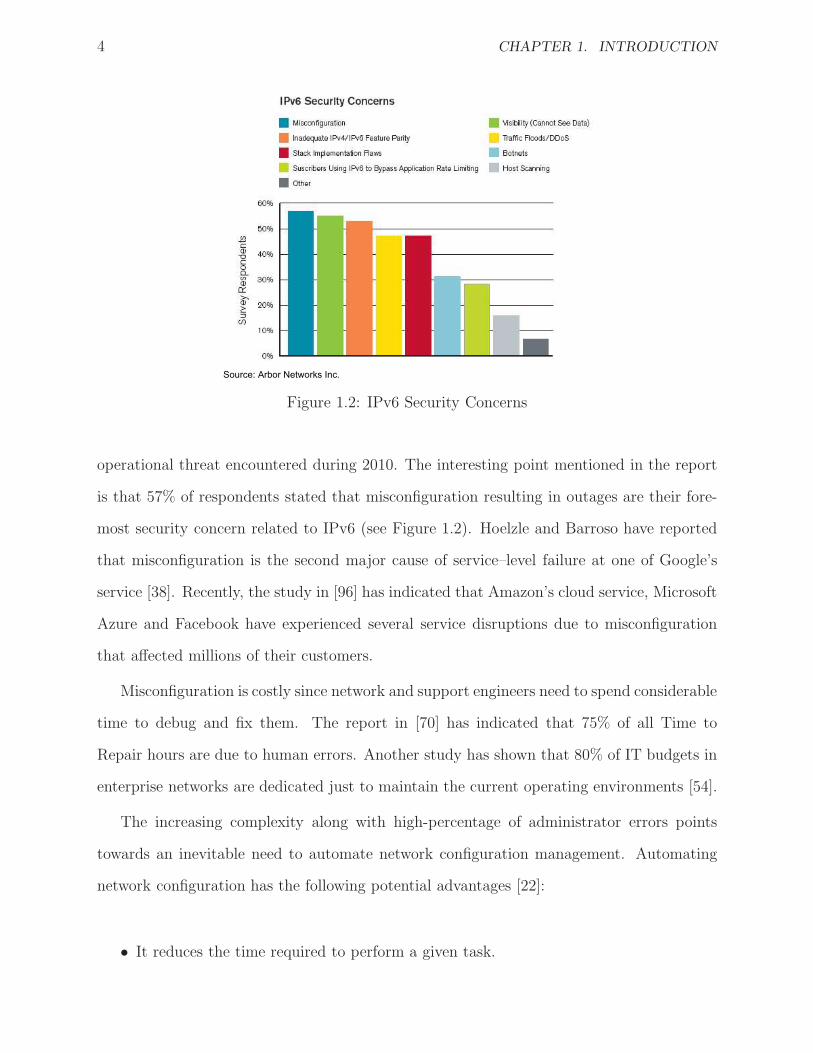
Source: Arbor Networks Inc.
Figure 1.2: IPv6 Security Concerns
operational threat encountered during 2010. The interesting point mentioned in the report
is that 57% of respondents stated that misconfiguration resulting in outages are their fore-
most security concern related to IPv6 (see Figure 1.2). Hoelzle and Barroso have reported
that misconfiguration is the second major cause of service–level failure at one of Google’s
service [38]. Recently, the study in [96] has indicated that Amazon’s cloud service, Microsoft
Azure and Facebook have experienced several service disruptions due to misconfiguration
that affected millions of their customers.
Misconfiguration is costly since network and support engineers need to spend considerable
time to debug and fix them. The report in [70] has indicated that 75% of all Time to
Repair hours are due to human errors. Another study has shown that 80% of IT budgets in
enterprise networks are dedicated just to maintain the current operating environments [54].
The increasing complexity along with high-percentage of administrator errors points
towards an inevitable need to automate network configuration management. Automating
network configuration has the following potential advantages [22]:
• It reduces the time required to perform a given task.
1.1. MOTIVATION 5
• It reduces the percentage of administrator error.
• It guarantees consistent configuration across an entire network.
• It provides accountability for changes.
The management of network devices is mostly performed by tools provided by the equip-
ment vendors. These tools are designed based on either the SNMP framework or proprietary
frameworks. SNMP-based tools have the limitation that they do not treat a network as a
uniform entity, but rather they interact with one network element at a time. Proprietary-
based tools have the limitation that they cannot be used in heterogeneous networks.
There are a plethora of other configuration management tools that simplify the configu-
ration of devices in an environment where there are a large number of heterogeneous devices.
These frameworks are centered on the idea of reducing complexity through abstraction and
separation of concerns. The objective of abstraction is to describe the operational require-
ments without diving down into how to achieve those requirements. However, due to the
sophistication of current network services, the ability to check and examine how a service is
configured is in fact critical to troubleshooting, debugging and quickly achieving the desired
effect. We believe that choosing the right level of abstraction is a key feature of a successful
management system. The abstraction should be low enough to the current configuration
management approach and high enough to capture the complexity of configuration tasks.
In 2006, the Internet Engineering Task Force (IETF) published a new configuration pro-
tocol called NETCONF [27]. In 2010, IETF published its associated data model, which
is known as YANG [11]. NETCONF resolves the limitations found in SNMP protocol and
together with YANG can make a powerful contribution in designing an efficient management
system . In fact, NETCONF and YANG are specifically designed for the task of network con-
figuration, and they are resulted from a series of recommendations of network operators and
experts. Several major network equipment vendors are already supporting these standards
in their devices [15]. Although, NETCONF and YANG provide a standardized abstraction
6 CHAPTER 1. INTRODUCTION
for low-level configuration tasks in multi–vendor networks, we still need to find a suitable
abstraction to close the gap between high–level requirements and NETCONF/YANG ab-
straction.
1.2 Problem Statement
Network configuration management is considered the most complicated task among other
network management tasks. The inadequacies of current network configuration approaches
have forced network operators to perform configuration tasks manually via CLIs. Several
studies have shown that misconfiguration is the most significant threat for network operation
and the main cause of network outage for many network environments. Moreover, networks
are configured to satisfy certain requirements. Requirements include performance, connec-
tivity, fault tolerance, security, provisioning, etc. The gap between high-level requirements
and low-level configuration data is difficult to close or bridge.
The aim of this dissertation is to develop an automated management system to enhance
network configuration management. Our objective is how to build a system that has the
following features:
• Scalability - It should accommodate all sizes of networks.
• Comprehensive - It should take into account the other management functions.
• Adaptable - It should accommodate new equipment or technology.
• Intelligent - It should minimize the human intervention by automating decision making.
• Interoperability - It should follow the standards to accommodate heterogeneous net-
work environments.

1.3. SCOPE 7
1.3 Scope
The scope of this dissertation is limited to improving network configuration management.
It does not focus on how to detect and analyze errors, how to assess network performance,
or how to guarantee service level agreement.
We assume that the management system has multiple subsystems that will handle the
other aspects of management functions, such as detecting faults, performance measuring, etc.
However, this dissertation provides a recommendation on how to develop such components
to work as a coherent complete system. The configuration management system relies on
these subsystems in order to maintain the network operational state.
The work in this dissertation is not focusing on systems management, which is pertaining
on anti-virus management, user’s activities, storage management, etc. Eventually, network
management environment is more stringent than systems management environment in the
sense that we do not have the freedom to install new software on network devices. We are
limited to the services that are provided on the network devices.
Finally, the work in this dissertation is limited for managing IP networks. It has limited
support for non-IP telecommunication networks.
1.4 Goals and Contributions
The dissertation describes a series of efforts to understand, manage, augment, verify and
automate network operations. The overarching goal is to build a comprehensive automated
configuration management system called AutoConf. AutoConf performs four management
functions: configuration change management, verification management, automation man-
agement and resource discovery management. Therefore, we summarize our contributions
as follows:
• Extensive literature review that covers the contributions of standard bodies in network
configuration management.

8 CHAPTER 1. INTRODUCTION
• Proposing a new configuration semantic model to logically link between the manage-
ment functions.
• A solution for resource discovery management based on NETCONF/YANG frame-
work.
• A comprehensive verification management that covers configuration data verification
and network behavior verification.
• A new set of formal models to represent firewall, routing and NAT policies.
• A solution for supporting dynamic networks based on reinforcement learning.
• A network topology generator tool to evaluate the scalability of AutoConf with large
networks.
• A policy–state generator tool to evaluate the efficiency of AutoConf to analyze large
set of policy rules and network state.
• A series of case studies on different configuration scenarios to illustrate the flexibility
of using AutoConf. The case studies include:
– RIP routing configuration,
– OSPF routing configuration,
– MPLS VLAN configuration, and
– Bridge configuration.
1.5 Organization
This dissertation is organized as follows. Chapter 2 provides the necessary background to
understand the concepts used in later chapters as well as a literature review. Chapter 3
defines the model and the framework that will be used to automate network configuration
1.5. ORGANIZATION 9
management. The automated system is divided into a set of components: change configu-
ration, verification analysis and configuration automation. The same chapter provides how
to handle configuration change. In Chapter 4, we describe the configuration verification
system. Then, we describe configuration automation in Chapter 5. The implementation of
AutoConf will be discussed in Chapter 6. In Chapter 7, we summarize our results where we
evaluate the AutoConf system on a set of case studies along with simulation models. We
conclude our dissertation in Chapter 8.

Chapter 2
Background and Literature Review
The design of our management system is built upon Binary Decision Diagram (BDD) and
reinforcement learning (RL) techniques. As such, we start this chapter with a quick in-
troduction to BDD and RL techniques. Then, we provide an overview of major network
management architectures and protocols. We focus on those architectures that have been
developed by standardized organizations such OSI, TMN and IETF. Our management sys-
tem uses the NETCONF protocol to communicate with managed devices. We give a detailed
description of the NETCONF protocol and its operations. We conclude this chapter by pre-
senting recent research work in network configuration management proposed in academia
and vendor operators’ communities.
2.1 Binary Decision Diagram
Network devices handle complex policies such as filtering, routing, etc. Let us consider the
following example that represents a filtering policy as shown in Table 2.1:
The example shows two rules. The first rule accepts any TCP traffic originated from
subnet 200.100.2.0/25 to the web servers in subnet 11.24.0.0/16. However, the second rule
denies any packet originated from subnet 200.100.2.0/25 when it tries to access ports from
11

12 CHAPTER 2. BACKGROUND AND LITERATURE REVIEW
constraint action
tcp 200.100.2.0 255.255.255.128 any 11.24.0.0 255.255.0.0 80 acceptany 200.100.2.0 255.255.255.128 any 11.24.0.0 255.255.0.0 1-1024 deny
Table 2.1: Sample of filtering policy
1 to 1024 of any machine in subnet 11.24.0.0/16. The order of filtering rules is critical.
If a packet matches the first rule, then it will be accepted. Otherwise, the packet will be
matched with the second rule. If we change the order of the two rules, then the first rule
will never be matched.
Network devices may store thousands of such rules. If a network has hundreds or thou-
sands of devices, how can we verify connectivity and security requirements? What should
our overall strategy be? Consider Figure 2.1 that shows a real and a formal worlds. Given
we want to find a real world solution as indicated by edge (1). However, in practice it is
hard to solve problems in the real world. One approach is to formalize the problem using a
formal model (edge 2). Within the formal world, we can solve the formal problem in feasible
time (edge 3), and transform the formal solution back to a real solution (edge 4).
Real Problem
Formal Problem Formal Soluton
Real Solution
(1)
(3)
(2) (4)
Figure 2.1: The real and formal worlds illustrated by two circles.
The route 2–3–4 might seem as detour over just taking edge 1. But going via the formal
world, we can quickly reason about our methods. In this dissertation, we use the Binary
decision diagram, or simply BDD, as our formal world.
Basically, BDD is a directed acyclic graph (DAG) data structure, which was introduced
2.1. BINARY DECISION DIAGRAM 13
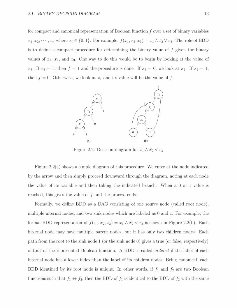
for compact and canonical representation of Boolean function f over a set of binary variables
x1, x2, · · · , xn where xi ∈ {0, 1}. For example, f(x1, x2, x3) = x1 ∧ x2 ∨ x3. The role of BDD
is to define a compact procedure for determining the binary value of f given the binary
values of x1, x2, and x3. One way to do this would be to begin by looking at the value of
x3. If x3 = 1, then f = 1 and the procedure is done. If x3 = 0, we look at x2. If x2 = 1,
then f = 0. Otherwise, we look at x1 and its value will be the value of f .
x3
x2
x1
1
0
10
10
10
0 1
x3
x2
x1
10
1
0
0 1
10
(a) (b)
Figure 2.2: Decision diagram for x1 ∧ x2 ∨ x3
Figure 2.2(a) shows a simple diagram of this procedure. We enter at the node indicated
by the arrow and then simply proceed downward through the diagram, noting at each node
the value of its variable and then taking the indicated branch. When a 0 or 1 value is
reached, this gives the value of f and the process ends.
Formally, we define BDD as a DAG consisting of one source node (called root node),
multiple internal nodes, and two sink nodes which are labeled as 0 and 1. For example, the
formal BDD representation of f(x1, x2, x3) = x1 ∧ x2 ∨ x3 is shown in Figure 2.2(b). Each
internal node may have multiple parent nodes, but it has only two children nodes. Each
path from the root to the sink node 1 (or the sink node 0) gives a true (or false, respectively)
output of the represented Boolean function. A BDD is called ordered if the label of each
internal node has a lower index than the label of its children nodes. Being canonical, each
BDD identified by its root node is unique. In other words, if f1 and f2 are two Boolean
functions such that f1 ↔ f2, then the BDD of f1 is identical to the BDD of f2 with the same
14 CHAPTER 2. BACKGROUND AND LITERATURE REVIEW
root node (given the same order of their binary variables).
BDDs allow logical operations on Boolean functions, such as AND, OR, and XOR, to be
performed in a polynomial time with respect to the number of nodes. Existing BDD packages
allow fast manipulation. In particular, the package that we use BuDDy [28] implements hash
tables along with cache memory for fast retrieving and traversing BDD graphs.
The main advantage of using Boolean function is to represent compactly complex con-
straints that compose of several conditions like the filtering policy shown in Table 2.1. This
research work uses BDD for this purpose. So, in the remaining of this section, we explain
how we model constraints using BDD.
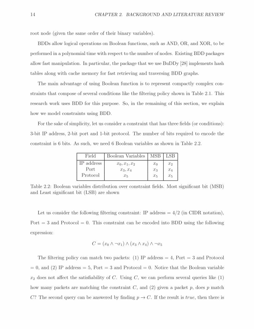
For the sake of simplicity, let us consider a constraint that has three fields (or conditions):
3-bit IP address, 2-bit port and 1-bit protocol. The number of bits required to encode the
constraint is 6 bits. As such, we need 6 Boolean variables as shown in Table 2.2.
Field Boolean Variables MSB LSB
IP address x0, x1, x2 x0 x2
Port x3, x4 x3 x4
Protocol x5 x5 x5
Table 2.2: Boolean variables distribution over constraint fields. Most significant bit (MSB)and Least significant bit (LSB) are shown
Let us consider the following filtering constraint: IP address = 4/2 (in CIDR notation),
Port = 3 and Protocol = 0. This constraint can be encoded into BDD using the following
expression:
C = (x0 ∧ ¬x1) ∧ (x3 ∧ x4) ∧ ¬x5
The filtering policy can match two packets: (1) IP address = 4, Port = 3 and Protocol
= 0, and (2) IP address = 5, Port = 3 and Protocol = 0. Notice that the Boolean variable
x2 does not affect the satisfiability of C. Using C, we can perform several queries like (1)
how many packets are matching the constraint C, and (2) given a packet p, does p match
C? The second query can be answered by finding p→ C. If the result is true, then there is

2.2. REINFORCEMENT LEARNING 15
a match. Also, notice that a Boolean function can have a very compact form when a field
has a range of values. For example, the network address 4/1 represents a subnetwork where
the first IP address is 4 and the last IP address is 7. The Boolean function to represent this
range of addresses is just x0.
2.2 Reinforcement Learning
Reinforcement Learning is a branch of Artificial Intelligence techniques for learning by inter-
action with an environment to accomplish a specific goal. There are three main components
in the RL framework: an agent, an environment and a scalar reward. The agent makes a
decision by taking an action at every time–step according to a policy and expects a feedback
in terms of a scalar reward for every action.
In RL literature, there are two types of problems where RL provides attractive solu-
tions [85]:
1. Policy evaluation, which refers to the techniques of evaluating the consequences of
taking actions according to a fixed policy, and
2. Policy control, which refers to the techniques of finding an optimal policy (π∗) that
maximizes the received rewards in a long run.
Therefore, in this dissertation, we just consider the techniques for solving control prob-
lems; specifically we consider RL techniques that are based on temporal difference (TD)
methods. They are used to find the optimal policy that does not require any assumption
except visiting all states in order to converge to optimal policy. The most well-known ap-
proaches that are based on TD are TD(λ), Sarsa and Q-learning. They offer a solution to
systems and networks management that differs from supervised machine learning techniques.
TD techniques can learn optimal policy with little or no built-in system-specific knowledge.
Later, we show the difference between TD(λ), Sarsa and Q-learning.
16 CHAPTER 2. BACKGROUND AND LITERATURE REVIEW
Several researches and case studies [88] have shown the promise of using TD in au-
tomating networks and systems management. In the following paragraphs, we give a formal
description of RL problems.
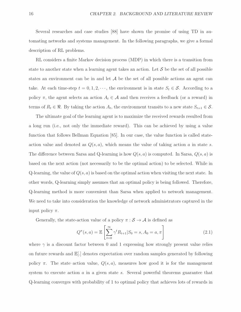
RL considers a finite Markov decision process (MDP) in which there is a transition from
state to another state when a learning agent takes an action. Let S be the set of all possible
states an environment can be in and let A be the set of all possible actions an agent can
take. At each time-step t = 0, 1, 2, · · · , the environment is in state St ∈ S. According to a
policy π, the agent selects an action At ∈ A and then receives a feedback (or a reward) in
terms of Rt ∈ ℜ. By taking the action At, the environment transits to a new state St+1 ∈ S.
The ultimate goal of the learning agent is to maximize the received rewards resulted from
a long run (i.e., not only the immediate reward). This can be achieved by using a value
function that follows Bellman Equation [85]. In our case, the value function is called state-
action value and denoted as Q(s, a), which means the value of taking action a in state s.
The difference between Sarsa and Q-learning is how Q(s, a) is computed. In Sarsa, Q(s, a) is
based on the next action (not necessarily to be the optimal action) to be selected. While in
Q-learning, the value ofQ(s, a) is based on the optimal action when visiting the next state. In
other words, Q-learning simply assumes that an optimal policy is being followed. Therefore,
Q-learning method is more convenient than Sarsa when applied to network management.
We need to take into consideration the knowledge of network administrators captured in the
input policy π.
Generally, the state-action value of a policy π : S → A is defined as
Qπ(s, a) = E
[
∞∑
t=0
γtRt+1|S0 = s, A0 = a, π
]
(2.1)
where γ is a discount factor between 0 and 1 expressing how strongly present value relies
on future rewards and E[.] denotes expectation over random samples generated by following
policy π. The state–action value, Q(s, a), measures how good it is for the management
system to execute action a in a given state s. Several powerful theorems guarantee that
Q-learning converges with probability of 1 to optimal policy that achieves lots of rewards in
2.2. REINFORCEMENT LEARNING 17
the long run. In this case, the optimal action at a given state is the action with the highest
Q(s, a) value. Therefore, the optimal action-value function, denoted as Q∗ is
Q∗(s, a)def= max
πQπ(s, a), ∀s ∈ S, ∀a ∈ A.
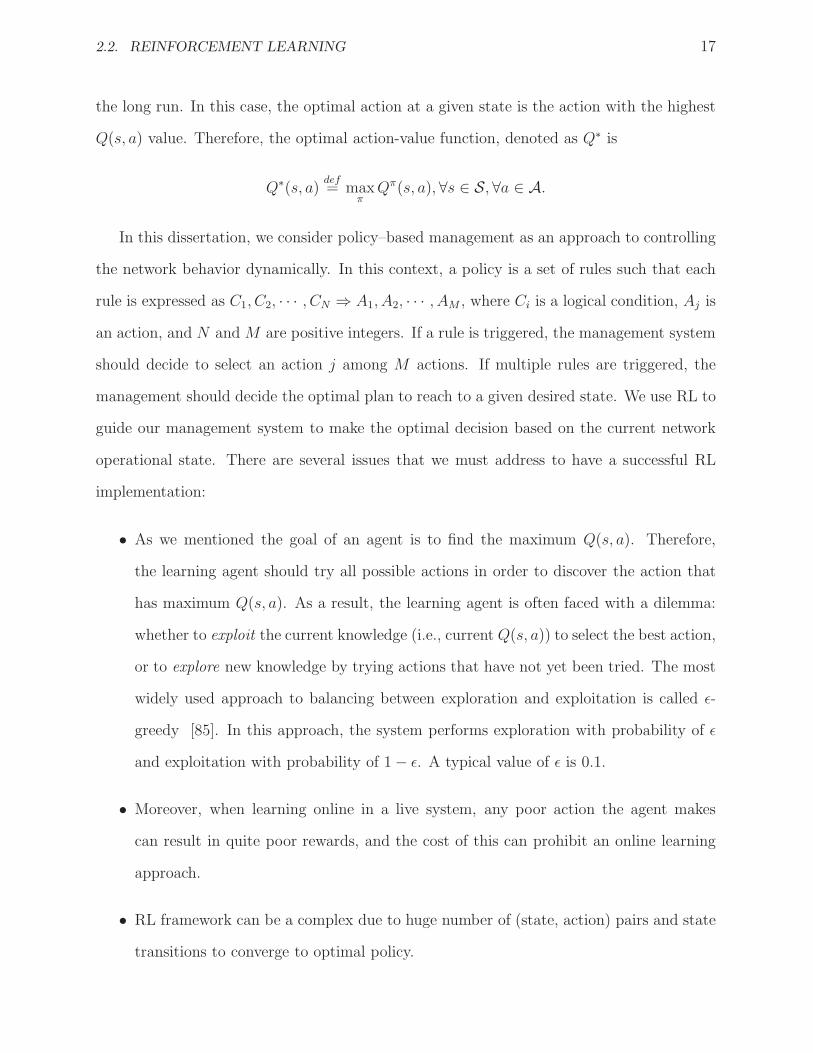
In this dissertation, we consider policy–based management as an approach to controlling
the network behavior dynamically. In this context, a policy is a set of rules such that each
rule is expressed as C1, C2, · · · , CN ⇒ A1, A2, · · · , AM , where Ci is a logical condition, Aj is
an action, and N and M are positive integers. If a rule is triggered, the management system
should decide to select an action j among M actions. If multiple rules are triggered, the
management should decide the optimal plan to reach to a given desired state. We use RL to
guide our management system to make the optimal decision based on the current network
operational state. There are several issues that we must address to have a successful RL
implementation:
• As we mentioned the goal of an agent is to find the maximum Q(s, a). Therefore,
the learning agent should try all possible actions in order to discover the action that
has maximum Q(s, a). As a result, the learning agent is often faced with a dilemma:
whether to exploit the current knowledge (i.e., current Q(s, a)) to select the best action,
or to explore new knowledge by trying actions that have not yet been tried. The most
widely used approach to balancing between exploration and exploitation is called ǫ-
greedy [85]. In this approach, the system performs exploration with probability of ǫ
and exploitation with probability of 1− ǫ. A typical value of ǫ is 0.1.
• Moreover, when learning online in a live system, any poor action the agent makes
can result in quite poor rewards, and the cost of this can prohibit an online learning
approach.
• RL framework can be a complex due to huge number of (state, action) pairs and state
transitions to converge to optimal policy.

18 CHAPTER 2. BACKGROUND AND LITERATURE REVIEW
In Q-learning, Equation 2.1 is approximated using the following expression:
Q(st, at)← Q(st, at) + α
[
Rt+1 + γmaxat+1
Q(st+1, at+1)−Q(st, at)
]
(2.2)
where α is called step size constant. However, we consider Dyna-Q approach (enhanced Q-
learning) since it has the capability to learn network’s dynamics on-line by building a partial
model plan [74, 84, 85]. It has been shown that Dyna-Q has significant accelerated learning
process. Briefly, Dyna-style learning is based on a model that is updated continually at each
time-step by navigating and propagating the action “goodness” to some steps in the history.
In Chapter 5, we discuss this algorithm further when we build an automated configuration
management system.
2.3 Network Management Architectures
This section analyzes the current technologies in network management in general while we
give more attention to the efforts that have been done in network configuration management.
We start with the efforts of organizations that have developed protocols and architectures
for network management. The well-known organizations that have significant contributions
to networks management are:
• The International Organizations for Standardization (ISO).
• The Telecommunication Standardization Sector (T) of the International Telecommu-
nication Union (ITU).
• The Internet Engineering Task Force (IETF).
• Distributed Management Task Force (DMTF).
Due to their efforts, networks, in essence, can be broadly classified into two categories:
telecommunication networks and IP networks. ISO and ITU-T provide solutions for telecom-
2.3. NETWORK MANAGEMENT ARCHITECTURES 19
munication networks while IETF provides solutions for IP networks. DMTF focuses on
systems management in enterprise IT environments.
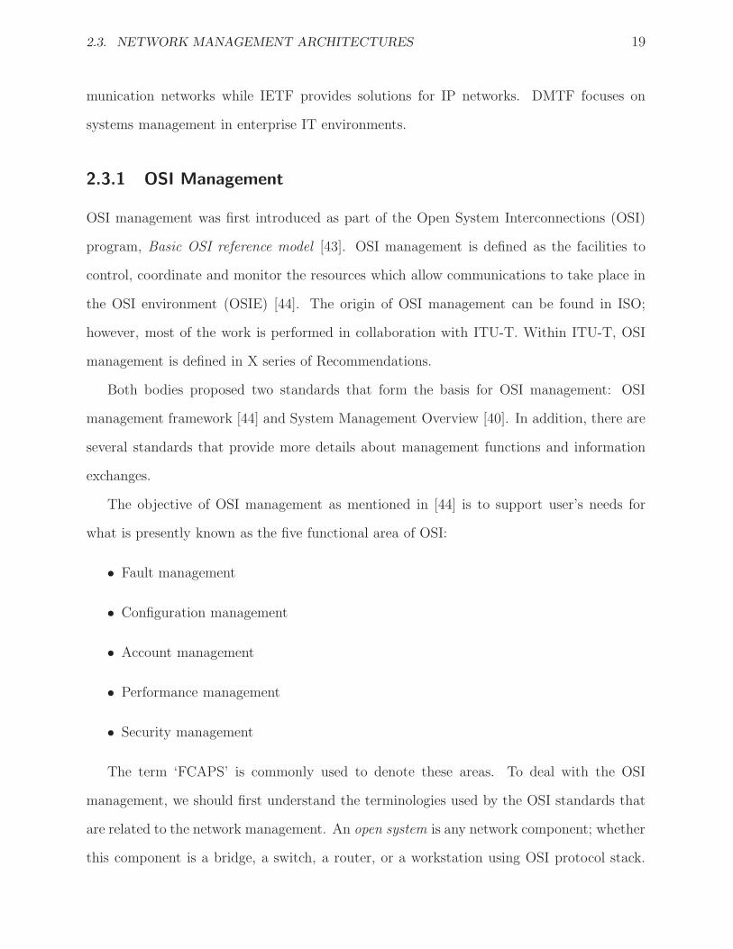
2.3.1 OSI Management
OSI management was first introduced as part of the Open System Interconnections (OSI)
program, Basic OSI reference model [43]. OSI management is defined as the facilities to
control, coordinate and monitor the resources which allow communications to take place in
the OSI environment (OSIE) [44]. The origin of OSI management can be found in ISO;
however, most of the work is performed in collaboration with ITU-T. Within ITU-T, OSI
management is defined in X series of Recommendations.
Both bodies proposed two standards that form the basis for OSI management: OSI
management framework [44] and System Management Overview [40]. In addition, there are
several standards that provide more details about management functions and information
exchanges.
The objective of OSI management as mentioned in [44] is to support user’s needs for
what is presently known as the five functional area of OSI:
• Fault management
• Configuration management
• Account management
• Performance management
• Security management
The term ‘FCAPS’ is commonly used to denote these areas. To deal with the OSI
management, we should first understand the terminologies used by the OSI standards that
are related to the network management. An open system is any network component; whether
this component is a bridge, a switch, a router, or a workstation using OSI protocol stack.
20 CHAPTER 2. BACKGROUND AND LITERATURE REVIEW
Any two devices that communicate via the OSI protocol at the same OSI Reference Model
layer are called peer open systems.
ISO in collaboration with ITU-T specifies four aspects to describe System Management
Model. These aspects are: information aspects, functional aspects, OSI communication
aspects, and organizational aspects. The following is a description for each aspect.
2.3.1.1 Information Aspects
The individual open system within the OSIE may have a set of resources that need to be
managed such as a layer entity, a connection, a physical communication equipment. These
resources are viewed as managed objects (MOs). That is, managed objects are abstractions
of data processing and data communications of resources for the purpose of management.
OSI MOs can be specific to an individual layer, in which case they are called (N)-layer MOs
managed by layer management protocol and services. Otherwise, they are called systems
MOs which are managed by system management protocol and services. The set of all
managed objects within an open system constitutes that system’s management information
base (MIB).
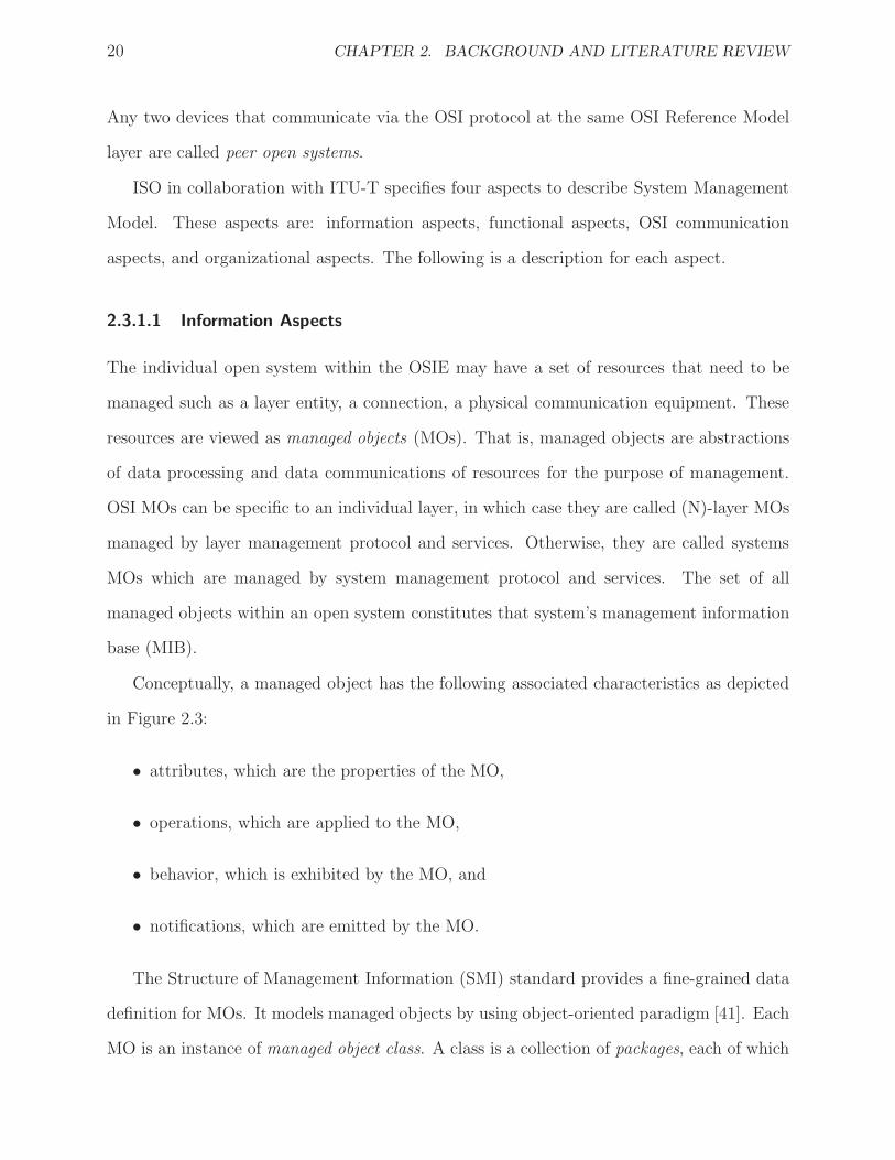
Conceptually, a managed object has the following associated characteristics as depicted
in Figure 2.3:
• attributes, which are the properties of the MO,
• operations, which are applied to the MO,
• behavior, which is exhibited by the MO, and
• notifications, which are emitted by the MO.
The Structure of Management Information (SMI) standard provides a fine-grained data
definition for MOs. It models managed objects by using object-oriented paradigm [41]. Each
MO is an instance of managed object class. A class is a collection of packages, each of which

2.3. NETWORK MANAGEMENT ARCHITECTURES 21
Attributes
Operations
Behaviors
Notifications
Figure 2.3: OSI abstraction for managed objects
is defined to be a collection of attributes, operations, behavior and notifications. Packages
are either mandatory or conditional upon some explicitly stated condition. When a new
MO is created, it must contain all mandatory packages and those packages for which the
explicit condition associated with them in the managed object class definition is evaluated
to TRUE.
Attributes are defined by using ASN.1 notation [47]. An attribute can be a single-valued
or a set-valued. A group of attributes sharing the same behavior can be aggregated together
to constitute a structured-valued attribute called attribute group. Moreover, an attribute
group can have a fixed set of attributes or an extensible set of attributes as a result of
inheritance.
SMI standard has defined two types of operations: operations related to MO’s attributes
and operations related to MO as a whole. The operations that can be applied to MO’s
attributes are:
• get: to retrieve an attribute value,
• replace: to modify an attribute value,
• replace-with-default: to replace an attribute value with its default value,
• add: to insert a member value to a set-valued attribute, and
• remove: to remove a member from a set-valued attribute.
The operations that can be applied to a MO as a whole are:
• create: to create new instances of the MO,

22 CHAPTER 2. BACKGROUND AND LITERATURE REVIEW
Fault
requirements
Configuration
requirements
Accounting
requirements
Performance
requirements
Security
requirements
MF MF MF MF MF
System management functions
Figure 2.4: Relationships between management functions and user requirements
• delete: to delete the MO, and
• action: for user-defined operation
Finally, a MO can exhibit any of the following behavior:
• Imposing semantic and consistency constraints on attributes.
• Establishing dependency relationship between attributes; taking into account the pres-
ence or absence of conditional packages,
• Determining how the MO responds when it receives management operations.
• Defining the situation under which notification will be triggered.
• Defining the preconditions and the postconditions that constraint the validity of op-
erations and notifications.
2.3.1.2 Functional Aspects
Management activities are modeled as a set of system management functions (MFs), each
of which is satisfying certain user requirements. For example, reading an error counter (as a
function) could be used for fault management or performance management. Similarly, a user
requirement may require more than one management function to be satisfied. Figure 2.4
shows many-to-many relationship between management functions and requirements.
ISO and ITU-T have developed a set of standards specifying standard system manage-
ment functions. Within ISO, management functions are defined in ISO/IEC 10164 while

2.3. NETWORK MANAGEMENT ARCHITECTURES 23
Title ISO/IEC ITU-T
Object management function 10164-1 X.730State management function 10164-2 X.731Attributes for representing relationships 10164-3 X.732Alarm reporting function 10164-4 X.733Event report management function 10164-5 X.734Log control function 10164-6 X.735Security log function 10164-7 X.736Security audit trail function 10164-8 X.740Objects and attributes for access control function 10164-9 X.741Usage metering function for accounting purpose 10164-10 X.742Metric objects and attributes 10164-11 X.739Test management function 10164-12 X.745Summarization function 10164-13 X.738Confidence and diagnostic test categories 10164-14 X.737Scheduling function 10164-15 X.746Management knowledge management function 10164-16 X.750Change over function 10164-17 X.751Software management function 10164-18 X.744Management domain and management policy management function 10164-19 X.749Time management function 10164-20 X.743Command sequencer for systems management 10164-21 X.753Response time monitoring function 10164-22 X.748
Table 2.3: Systems management functions
within ITU-T, they are defined in ITU-T X.730-799 recommendations series. Table 2.3
shows a list of defined management functions.
2.3.1.3 Organizational Aspects
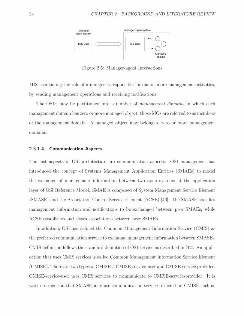
OSI System management model follows the agent-manager paradigm as shown in Figure 2.5.
In case of management system, management activities are carried out by management infor-
mation services (MIS-users). Management information is exchanged between two MIS-users
only when one MIS-user is acting as the agent role and the other is acting as the manager
role. MIS-user’s role is not static. An MIS-user can change its role over time.
An MIS-user taking the role of an agent is responsible to process the received management
operations on MOs. It may also forward notifications emitted by MOs to a manager. An
24 CHAPTER 2. BACKGROUND AND LITERATURE REVIEW
MIS-User
Managed open systemManager
open system
MIS-User
Managed
objects
Figure 2.5: Manager-agent Interactions
MIS-user taking the role of a manger is responsible for one or more management activities,
by sending management operations and receiving notifications.
The OSIE may be partitioned into a number of management domains in which each
management domain has zero or more managed object; those MOs are referred to as members
of the management domain. A managed object may belong to zero or more management
domains.
2.3.1.4 Communication Aspects
The last aspects of OSI architecture are communication aspects. OSI management has
introduced the concept of Systems Management Application Entities (SMAEs) to model
the exchange of management information between two open systems at the application
layer of OSI Reference Model. SMAE is composed of System Management Service Element
(SMASE) and the Association Control Service Element (ACSE) [46]. The SMASE specifies
management information and notifications to be exchanged between peer SMAEs, while
ACSE establishes and closes associations between peer SMAEs.
In addition, OSI has defined the Common Management Information Service (CMIS) as
the preferred communication service to exchange management information between SMASEs.
CMIS definition follows the standard definition of OSI-service as described in [42]. An appli-
cation that uses CMIS services is called Common Management Information Service Element
(CMISE). There are two types of CMISEs: CMISE-service-user and CMISE-service provider.
CMISE-service-user uses CMIS services to communicate to CMISE-service-provider. It is
worth to mention that SMASE may use communication services other than CMISE such as
2.3. NETWORK MANAGEMENT ARCHITECTURES 25
File Transfer, Access and Management (FTAM) [45] or Transaction Processing (TP) [39].
The CMIS standard defines the following service primitives:
• M-GET : to retrieve management information.
• M-CANCEL-GET : to cancel a previously invoked M-GET. If, for example, M-GET
delivers too much information such an entire routing table, a manager can send M-
CANCEL-GET to stop the transmission
• M-SET : to modify an attribute or a set of attributes of a MO.
• M-ACTION : to perform some actions defined on a MO.
• M-CREATE : to create a new instance of a MO.
• M-DELETE : to delete an existing MO.
• M-EVENT-REPORT : to report the occurrence of some kind of events as a notification.
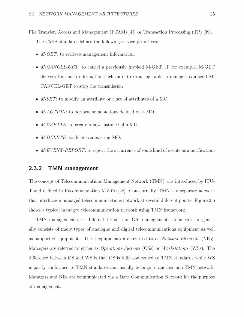
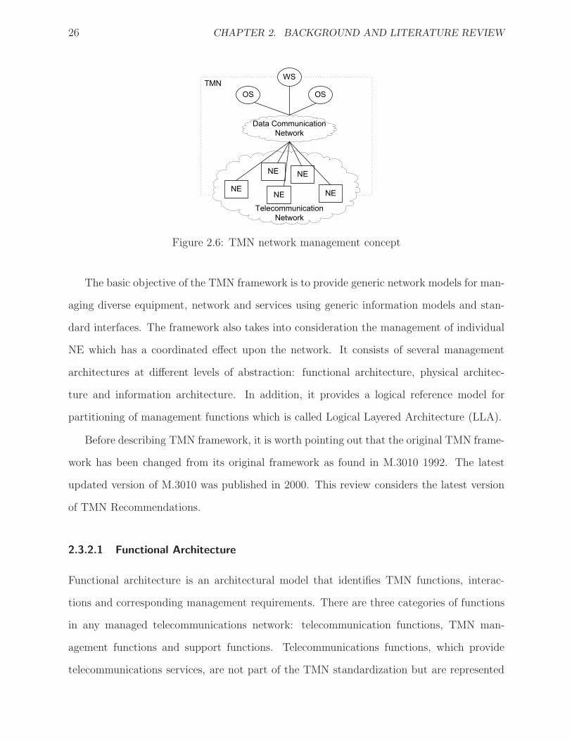
2.3.2 TMN management
The concept of Telecommunications Management Network (TMN) was introduced by ITU-
T and defined in Recommendation M.3010 [48]. Conceptually, TMN is a separate network
that interfaces a managed telecommunications network at several different points. Figure 2.6
shows a typical managed telecommunication network using TMN framework.
TMN management uses different terms than OSI management. A network is gener-
ally consists of many types of analogue and digital telecommunications equipment as well
as supported equipment. These equipments are referred to as Network Elements (NEs).
Managers are referred to either as Operations Systems (OSs) or Workstations (WSs). The
difference between OS and WS is that OS is fully conformed to TMN standards while WS
is partly conformed to TMN standards and usually belongs to another non-TMN network.
Managers and NEs are communicated via a Data Communication Network for the purpose
of management.
26 CHAPTER 2. BACKGROUND AND LITERATURE REVIEW
NE
NE
NE
NE
NE
OS
WS
OS
Data Communication
Network
TMN
Telecommunication
Network
Figure 2.6: TMN network management concept
The basic objective of the TMN framework is to provide generic network models for man-
aging diverse equipment, network and services using generic information models and stan-
dard interfaces. The framework also takes into consideration the management of individual
NE which has a coordinated effect upon the network. It consists of several management
architectures at different levels of abstraction: functional architecture, physical architec-
ture and information architecture. In addition, it provides a logical reference model for
partitioning of management functions which is called Logical Layered Architecture (LLA).
Before describing TMN framework, it is worth pointing out that the original TMN frame-
work has been changed from its original framework as found in M.3010 1992. The latest
updated version of M.3010 was published in 2000. This review considers the latest version
of TMN Recommendations.
2.3.2.1 Functional Architecture
Functional architecture is an architectural model that identifies TMN functions, interac-
tions and corresponding management requirements. There are three categories of functions
in any managed telecommunications network: telecommunication functions, TMN man-
agement functions and support functions. Telecommunications functions, which provide
telecommunications services, are not part of the TMN standardization but are represented

2.3. NETWORK MANAGEMENT ARCHITECTURES 27
to the TMN for the purpose to be managed. TMN management functions are responsible
to monitor and control the telecommunications network as well as the TMN network itself.
Support functions, which may optionally be found in the TMN, provide additional func-
tionality to support the management functions such as data communication functionality,
database functionality, user interface functionality and security functionality.
Functional architecture provides a conceptual model of TMN functionality and has the
following fundamental elements:
• Function blocks,
• Management Application Function,
• TMN management function sets, and
• Reference points.
In the following paragraphs, we give a brief description for each element.
Function blocks. Function blocks organize management functionality based on the role of
its functions. TMN standard defines a function block as the smallest deployable structure
of TMN management functionality. There are four types of function blocks:
• Operations Systems Function block (OSF), which includes management functions to
manage and control NEs and TMN itself (other OSs).
• Network Element Function block (NEF), which provides telecommunication and sup-
port functions to facilitate OSF to manage NEs.
• Workstation Function block (WSF), which supports WSs to translate between a TMN
reference point and a non-TMN reference point.
• Transformation Function block (TF), which connects between two functional entities
with incompatible communication mechanism. The TF may be used to connect two
28 CHAPTER 2. BACKGROUND AND LITERATURE REVIEW
MAF
MAF
Support functions
Function block
communication
Function block
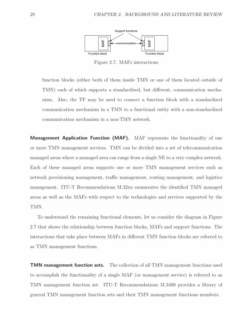
Figure 2.7: MAFs interactions
function blocks (either both of them inside TMN or one of them located outside of
TMN) each of which supports a standardized, but different, communication mecha-
nism. Also, the TF may be used to connect a function block with a standardized
communication mechanism in a TMN to a functional entity with a non-standardized
communication mechanism in a non-TMN network.
Management Application Function (MAF). MAF represents the functionality of one
or more TMN management services. TMN can be divided into a set of telecommunication
managed areas where a managed area can range from a single NE to a very complex network.
Each of these managed areas supports one or more TMN management services such as
network provisioning management, traffic management, routing management, and logistics
management. ITU-T Recommendations M.32xx enumerates the identified TMN managed
areas as well as the MAFs with respect to the technologies and services supported by the
TMN.
To understand the remaining functional elements, let us consider the diagram in Figure
2.7 that shows the relationship between function blocks, MAFs and support functions. The
interactions that take place between MAFs in different TMN function blocks are referred to
as TMN management functions.
TMN management function sets. The collection of all TMN management functions used
to accomplish the functionality of a single MAF (or management service) is referred to as
TMN management function set. ITU-T Recommendations M.3400 provides a library of
general TMN management function sets and their TMN management functions members.

2.3. NETWORK MANAGEMENT ARCHITECTURES 29
NEF OSF TF WSF non-TMN
NEF q qOSF q q or x q fTF q q q f mWSF f f g
non-TMN m g
Table 2.4: Relation between function blocks expressed as reference points
Reference points. The concept of reference points was introduced to standardize the inter-
actions between function blocks. A reference point represents an external view of a particular
pair of function blocks. Different external views have been defined. One external view is
the aggregation of all abilities offered by a particular function block to another function
block. A second external view is the aggregation of all management operations between
function blocks. A third external view is the aggregation of all notifications emitted from
one function block to another function block.
Five different classes of reference points are identified. Three of them (q, f and x) are
TMN reference points; the other classes (g and m) are non-TMN reference points. The
relationship between reference points and function blocks is illustrated in Table 2.4. The
table illustrates all of possible pairs of TMN function blocks that can be associated via
a reference point. A function block at the top of a column may exchange management
information with a function block at the left of a row over the reference point that is
mentioned at the intersection of the column and row. if the intersection is empty, the
associated function blocks cannot directly exchange management information between each
other. Reference point x is applied only when each OSF is in different TMN.
2.3.2.2 Information Architecture
For information architecture, TMN standardization did not develop its own specific in-
formation model but built upon industry recognized solutions that are based on object-
oriented paradigm such as OSI management information model and CORBA-based infor-
30 CHAPTER 2. BACKGROUND AND LITERATURE REVIEW
mation model.
2.3.2.3 Physical Architecture
The purpose of physical architecture is to implement the functional architecture where the
implementations rely on the underlying physical equipment. Therefore, TMN physical ar-
chitecture is defined at a lower abstraction level than TMN functional architecture.
The physical model has the following fundamental elements: building blocks (physical
equipment) and interfaces. A building block is responsible to implement at least one function
block while interfaces are responsible to implement reference points. The physical model
defines seven building blocks:
• Operations System (OS), which implements OSFs(m)1 as well as TFs and WSFs.
• Q-Adapter device (QA), which implements TFs when TFs connect a TMN function
block with a non-TMN function block at m interface having TMN communication
standard.
• X-Adapter device (XA), which implements TFs when TFs connect a TMN function
block with a non-TMN function block having non-TMN communication standard.
• Q-Mediator device (QM), which implements TFs when TFs connect between TMN
function blocks having incompatible communication mechanism and both function
blocks are on the same TMN.
• X-Mediator device (QM), which implements TFs when TFs connect between TMN
function blocks on different TMN having incompatible communication mechanism.
• Network Element (NE), which implements NEFs(m) as well as TF, OSF and WSF.
• Workstation (WS), which implements WSFs only.
1m between parenthesis means mandatory
2.3. NETWORK MANAGEMENT ARCHITECTURES 31
OSF
OSF
OSF
OSF
NEF
Business Management Layer
Service Management Layer
Network Management Layer
Element Management Layer
Network Element Layer
q
q
q
q
Figure 2.8: TMN Functional Layering
In order for two or more physical blocks to exchange management information, they
must agree on a unified interface to communicate. We can imagine interfaces as the im-
plementations of communication services within the protocol stacks. TMN standardization
defines three interfaces corresponding to the reference point that implements: Q interface,
F interface and X interface.
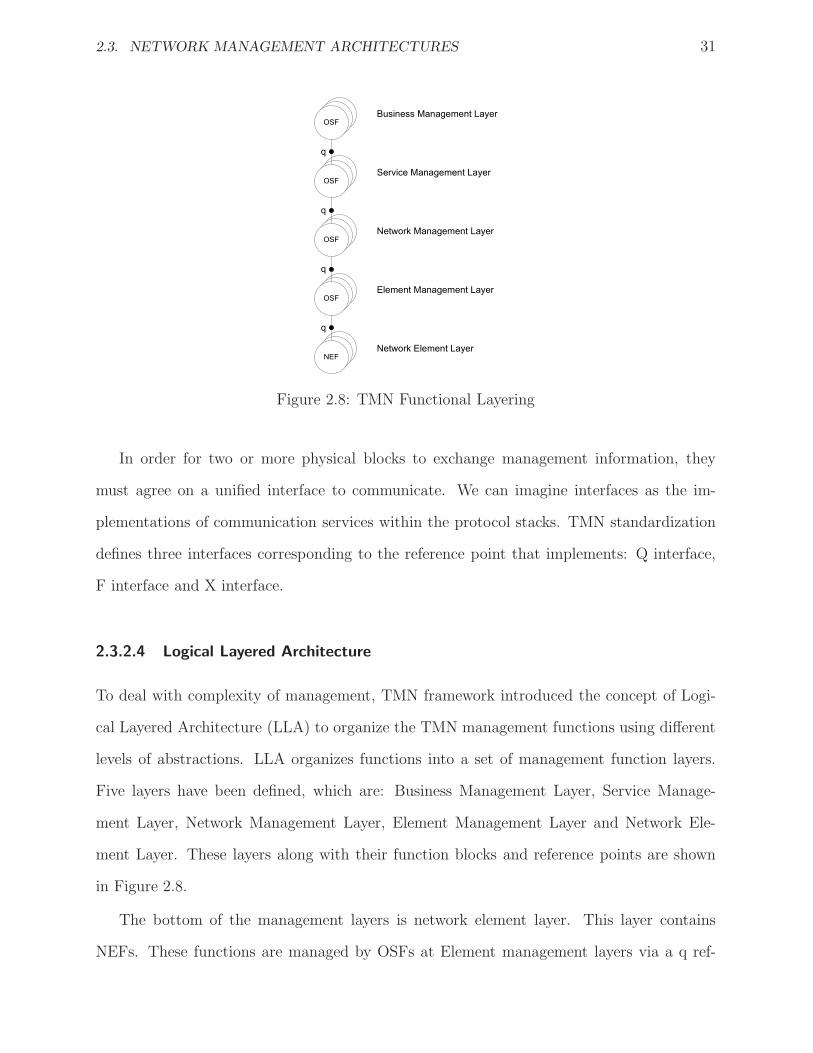
2.3.2.4 Logical Layered Architecture
To deal with complexity of management, TMN framework introduced the concept of Logi-
cal Layered Architecture (LLA) to organize the TMN management functions using different
levels of abstractions. LLA organizes functions into a set of management function layers.
Five layers have been defined, which are: Business Management Layer, Service Manage-
ment Layer, Network Management Layer, Element Management Layer and Network Ele-
ment Layer. These layers along with their function blocks and reference points are shown
in Figure 2.8.
The bottom of the management layers is network element layer. This layer contains
NEFs. These functions are managed by OSFs at Element management layers via a q ref-

32 CHAPTER 2. BACKGROUND AND LITERATURE REVIEW
erence point. Element OSFs, which concerns the management of individual NE, in turns,
are managed by OSFs at network management layer. Network OSFs cover the realization
of network-based TMN application functions by interacting with Elements OSFs. Thus, the
Element and Network OSFs provide the functionality to manage a network by coordinating
activities across the network and supporting the services offered by the network. Service
management layer concerns with services offered by one or more networks and normally
performs a customer interfacing. Finally, business management layer concerns with the
management of the whole enterprise and carries out an overall business coordination.
2.3.3 Internet Management
The concept of Internet-based management was introduced by Internet Engineering Task
Force (IETF). In contrast to OSI approach, IETF did not define a specialized standard for
Internet Management Architecture. Current Internet management architectures are tailored
based on the underlying communication protocols. The main two communication protocols
defined by IETF for the purpose of exchanging management information are Simple Network
Management Protocol (SNMP) and NETwork CONFiguration Protocol (NETCONF).
The Internet management architecture that is based on SNMP framework is called In-
ternet Standard Management Framework or simply SNMP framework. For the NETCONF,
up to writing this dissertation, there is no proposed management architecture for NET-
CONF. Therefore, the remaining of this section will concentrate on the Internet Standard
Management Framework.
IETF has defined three versions of Simple Network Management Protocol: SNMPv1,
SNMPv2 and SNMPv3. Regardless of SNMP versions, the fundamental elements of Internet
Standard Management Framework are the same in the three versions [17], which are:
• A set of SNMP entities that take either the role of agent or manager. An SNMP entity
with the role of agent provides remote access to SNMP entity with the role of manager.
Moreover, management applications are executed at the manager side.
2.3. NETWORK MANAGEMENT ARCHITECTURES 33
• A management protocol to exchange management information.
• Management information.
The specifications of the Internet Standard Management Framework are entirely information-
oriented. The framework consists of the followings:
• A data definition language called Structure of Management Information (SMI).
• A definition of management information or Management Information Base (MIB).
• A definition of a protocol for information exchange called Simple Network Management
Protocol (SNMP).
• Security and Administration.
2.3.3.1 Structure of Management Information (SMI)
The SMI defines precisely how managed objects are described and named for the purpose of
management. SMI notations are taken from OSI’s ASN.1 language. There are two versions
of the SMI: SMIv1 and SMIv2. SMIv1 is described in RFCs 1155, 1212 and 1215 while
SMIv2 is described in RFCs 2578, 2579 and 2580. SMIv2 extends SMIv1 by adding new
data types, enhancing object definition and adding SNMPv2 node to MIB tree as we will
explain later. The SMI is divided into three parts:
• Module definitions, which are used to define information modules using the SMI no-
tation MODULE-IDENTITY.
• Object definitions, which are used to describe and name managed objects. Object
definition starts with the SMI notation OBJECT-TYPE.
• Notification definitions, which are used to define events emitted by SNMP agent entity.
Notification definition starts with the SMI notation NOTIFICATION-TYPE.

34 CHAPTER 2. BACKGROUND AND LITERATURE REVIEW
Root Node
iso(1)ccit(0) joint(2)
org(3)
DoD (6)
Internet(1)directory(1)
management
(2)
experimental
(3)private(4) security(5)
SNMPv2 (6)
Mail(7)
MIB-II(1)
enterprises(1)
Figure 2.9: SMI object tree
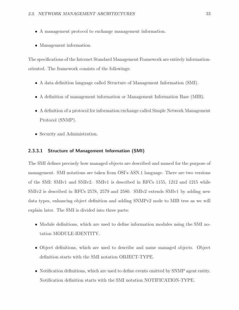
To uniquely identify each managed object, the SMI introduces a naming scheme, which
is basically a tree-like hierarchy. The top of the tree is called the root node and the leaves
represent the actual management variables or information to be monitored or controlled.
Except the root node, each node in the tree has a name and an integer number. An object
ID is made up of a series of integers separated by dots based on traversing the tree starting
from the root node and ending at the leaf node. Figure 2.9 shows a few top levels of this
MIB tree.
2.3.3.2 Management Information Base (MIB)
To identify all managed objects that can be controlled and monitored, a large number of
Management Information Base (MIB) standards have been developed. Among these MIBs
is MIB-II defined in RFC 1213. MIB-II is considered the most important and probably best
known MIB; it contains all information to manage the basic TCP/IP protocol suite. The
structure of this MIB is simple: management information that belongs to the same protocol
is aggregated together to form a group. There are nine groups defined in MIB-II: system
group, interfaces group, the address translation group, the IP group, the ICMP group,
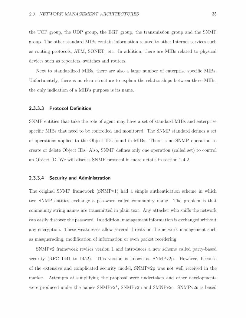
2.3. NETWORK MANAGEMENT ARCHITECTURES 35
the TCP group, the UDP group, the EGP group, the transmission group and the SNMP
group. The other standard MIBs contain information related to other Internet services such
as routing protocols, ATM, SONET, etc. In addition, there are MIBs related to physical
devices such as repeaters, switches and routers.
Next to standardized MIBs, there are also a large number of enterprise specific MIBs.
Unfortunately, there is no clear structure to explain the relationships between these MIBs;
the only indication of a MIB’s purpose is its name.
2.3.3.3 Protocol Definition
SNMP entities that take the role of agent may have a set of standard MIBs and enterprise
specific MIBs that need to be controlled and monitored. The SNMP standard defines a set
of operations applied to the Object IDs found in MIBs. There is no SNMP operation to
create or delete Object IDs. Also, SNMP defines only one operation (called set) to control
an Object ID. We will discuss SNMP protocol in more details in section 2.4.2.
2.3.3.4 Security and Administration
The original SNMP framework (SNMPv1) had a simple authentication scheme in which
two SNMP entities exchange a password called community name. The problem is that
community string names are transmitted in plain text. Any attacker who sniffs the network
can easily discover the password. In addition, management information is exchanged without
any encryption. These weaknesses allow several threats on the network management such
as masquerading, modification of information or even packet reordering.
SNMPv2 framework revises version 1 and introduces a new scheme called party-based
security (RFC 1441 to 1452). This version is known as SNMPv2p. However, because
of the extensive and complicated security model, SNMPv2p was not well received in the
market. Attempts at simplifying the proposal were undertaken and other developments
were produced under the names SNMPv2*, SNMPv2u and SMNPv2c. SNMPv2u is based
36 CHAPTER 2. BACKGROUND AND LITERATURE REVIEW
SNMP Entity
Dispatcher
SNMP Engine
Message
Processing
Subsystem
Security
Subsystem
Access
Control
Subsystem
Application
Command generator
Command responder
Notification receiver
Notification originator
Proxy forwarder
Other
Figure 2.10: SNMPv3 Entity
on a user-oriented security model while SNMPv2c is based on community strings similar to
SNMPv1 [37]. Needless to say, this proliferation resulted in market confusion and motivated
IETF to introduce SNMPv3.
SNMPv3 is the latest version of SNMP. Its main contribution to network management is
security. It provides message integrity, authentication and encryption. SNMPv3 introduces
two concepts: security model and security level. Security model is an authentication strategy
that is set up for a user and a group in which the user resides. A security level is the permitted
level of security within a security model. Together will determine which security mechanism
is employed when exchanging management information [25].
SNMPv3 entity has a single engine to perform the message processing as shown in Fig-
ure 2.10. When an application wants to send SNMP PDUs to the other SNMP entity, the
engine first accepts the SNMP datagram to be sent from SNMP application level, performs
the appropriate security functions, encapsulates the PDU into an SNMPv3 message, and
finally dispatches the message out to the network. When the engine receives an SNMPv3
message from the network, it performs the necessary decryption and authentication functions
before passing the PDU to the SNMP applications.
2.3. NETWORK MANAGEMENT ARCHITECTURES 37
2.3.4 Discussion and Critique
This section discusses some of the main problems found in the current network management
architectures. The aim of this discussion is to shed some lights on the weaknesses of these
architectures that will be tackled in this dissertation. We start with the problems of OSI
management, then TMN management and finally Internet management.
OSI management does not follow the principle of ISO Reference Model in which the
users in a particular layer has no information about other layers. However, SMAE entity at
application layer can access managed objects in other layers. Another weak point of OSI’s
framework is that the layer protocols (such as the presentation layer or transport layer) that
are being managed, are used for exchanging management information too. This dependence
contradicts the coherence of the framework since SMAE application cannot send ALARM
report due to a failure in the transport layer.
TMN management architecture has several advantages over OSI management. First,
TMN management assumes a separation between the telecommunication network that is
managed and the TMN network that transfers management information. Such separation
resolves the last problem we mentioned in previous paragraph. However, having a separate
network for TMN requires additional equipment and transmission media. In addition, TMN
needs to be managed, which introduces an extra overhead.
The second advantage of TMN over OSI management is that TMN defines multiple
architectures as opposed to OSI management, which defines only a single management ar-
chitecture. Having multiple architectures is useful when handling an additional, orthogonal
issue.
The last advantage of TMN is that it divides the management responsibilities into mul-
tiple layers as we discussed in Section 2.3.2.4. Having such layers, it becomes easier to
distinguish various management activities that exist in real networks.
For Internet management, IETF did not define an independent standard for Internet
management architecture, but rather the architecture is defined based on SNMP architec-
38 CHAPTER 2. BACKGROUND AND LITERATURE REVIEW
ture. SNMP architecture is information–oriented. The main disadvantage of SNMP archi-
tecture is the lack of a functional structure to classify thousands of management variables
(defined in MIB). One advantage of SNMP architecture over other architectures is that
management systems that are based on SNMP are much less expensive than management
systems that are based on OSI or TMN architectures.
By analyzing the above architectures, the main issue with network management frame-
works is the inability to express the requirement rules and policies, which make it impossible
to use these technologies to directly change the configuration of network elements in response
to a new or altered high-level requirements [81]. Our solution proposes multi-layer framework
that establishes relationships between semantically-related network devices. Such relation-
ships enable network administrators to easily express the network requirements and facilitate
the automation of network configuration management.
2.4 Network Management Protocols
In this section, we consider the network management protocols that are related to network
configuration management. Up to present, there are three standards of network configura-
tion management protocols: Common Management Information Protocol (CMIP), Simple
Network Management Protocol (SNMP), and Network Configuration Protocol (NETCONF).
2.4.1 Common Management Information Protocol
Common Management Information Protocol (CMIP) is an application layer protocol based
on OSI reference model defined in ISO/IEC 9596-1 (ITU-T X.711) [57]. It provides an
implementation for the services defined by CMIS. The specification of this protocol explains
in detail the manner in which the protocol should perform for each of the CMIS services.
The CMIP protocol requires that each application entity has a CMIP machine (CMIPM)
to implement CMIP protocol. CMIPM performs two functions: First, it accepts CMIS
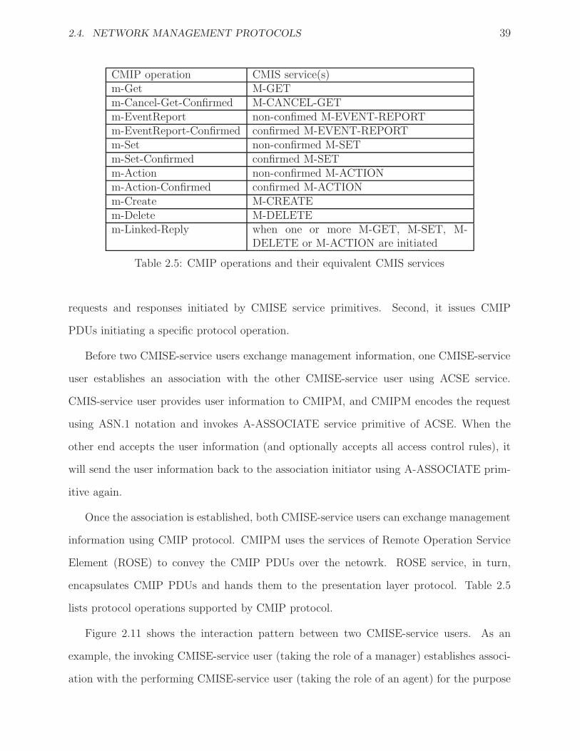
2.4. NETWORK MANAGEMENT PROTOCOLS 39
CMIP operation CMIS service(s)m-Get M-GETm-Cancel-Get-Confirmed M-CANCEL-GETm-EventReport non-confimed M-EVENT-REPORTm-EventReport-Confirmed confirmed M-EVENT-REPORTm-Set non-confirmed M-SETm-Set-Confirmed confirmed M-SETm-Action non-confirmed M-ACTIONm-Action-Confirmed confirmed M-ACTIONm-Create M-CREATEm-Delete M-DELETEm-Linked-Reply when one or more M-GET, M-SET, M-
DELETE or M-ACTION are initiated
Table 2.5: CMIP operations and their equivalent CMIS services
requests and responses initiated by CMISE service primitives. Second, it issues CMIP
PDUs initiating a specific protocol operation.
Before two CMISE-service users exchange management information, one CMISE-service
user establishes an association with the other CMISE-service user using ACSE service.
CMIS-service user provides user information to CMIPM, and CMIPM encodes the request
using ASN.1 notation and invokes A-ASSOCIATE service primitive of ACSE. When the
other end accepts the user information (and optionally accepts all access control rules), it
will send the user information back to the association initiator using A-ASSOCIATE prim-
itive again.
Once the association is established, both CMISE-service users can exchange management
information using CMIP protocol. CMIPM uses the services of Remote Operation Service
Element (ROSE) to convey the CMIP PDUs over the netowrk. ROSE service, in turn,
encapsulates CMIP PDUs and hands them to the presentation layer protocol. Table 2.5
lists protocol operations supported by CMIP protocol.
Figure 2.11 shows the interaction pattern between two CMISE-service users. As an
example, the invoking CMISE-service user (taking the role of a manager) establishes associ-
ation with the performing CMISE-service user (taking the role of an agent) for the purpose
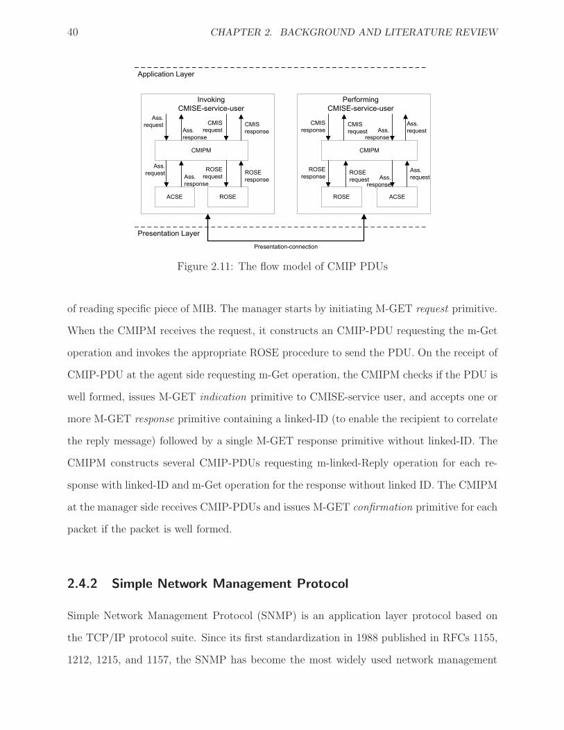
40 CHAPTER 2. BACKGROUND AND LITERATURE REVIEW
ACSE ROSE
Invoking
CMISE-service-user
CMIPM
CMIS
response
ROSE
response
ROSE
request
CMIS
request
Application Layer
Presentation Layer
ACSEROSE
Performing
CMISE-service-user
CMIPM
CMIS
request
ROSE
request
ROSE
response
CMIS
response
Presentation-connection
Ass.
request
Ass.
requestAss.
request
Ass.
request
Ass.
response
Ass.
response
Ass.
response
Ass.
response
Figure 2.11: The flow model of CMIP PDUs
of reading specific piece of MIB. The manager starts by initiating M-GET request primitive.
When the CMIPM receives the request, it constructs an CMIP-PDU requesting the m-Get
operation and invokes the appropriate ROSE procedure to send the PDU. On the receipt of
CMIP-PDU at the agent side requesting m-Get operation, the CMIPM checks if the PDU is
well formed, issues M-GET indication primitive to CMISE-service user, and accepts one or
more M-GET response primitive containing a linked-ID (to enable the recipient to correlate
the reply message) followed by a single M-GET response primitive without linked-ID. The
CMIPM constructs several CMIP-PDUs requesting m-linked-Reply operation for each re-
sponse with linked-ID and m-Get operation for the response without linked ID. The CMIPM
at the manager side receives CMIP-PDUs and issues M-GET confirmation primitive for each
packet if the packet is well formed.
2.4.2 Simple Network Management Protocol
Simple Network Management Protocol (SNMP) is an application layer protocol based on
the TCP/IP protocol suite. Since its first standardization in 1988 published in RFCs 1155,
1212, 1215, and 1157, the SNMP has become the most widely used network management
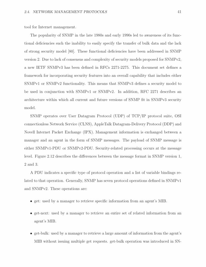
2.4. NETWORK MANAGEMENT PROTOCOLS 41
tool for Internet management.
The popularity of SNMP in the late 1980s and early 1990s led to awareness of its func-
tional deficiencies such the inability to easily specify the transfer of bulk data and the lack
of strong security model [80]. These functional deficiencies have been addressed in SNMP
version 2. Due to lack of consensus and complexity of security models proposed for SNMPv2,
a new IETF SNMPv3 has been defined in RFCs 2271-2275. This document set defines a
framework for incorporating security features into an overall capability that includes either
SNMPv1 or SNMPv2 functionality. This means that SNMPv3 defines a security model to
be used in conjunction with SNMPv1 or SNMPv2. In addition, RFC 2271 describes an
architecture within which all current and future versions of SNMP fit in SNMPv3 security
model.
SNMP operates over User Datagram Protocol (UDP) of TCP/IP protocol suite, OSI
connectionless Network Service (CLNS), AppleTalk Datagram-Delivery Protocol (DDP) and
Novell Internet Packet Exchange (IPX). Management information is exchanged between a
manager and an agent in the form of SNMP messages. The payload of SNMP message is
either SNMPv1-PDU or SNMPv2-PDU. Security-related processing occurs at the message
level. Figure 2.12 describes the differences between the message format in SNMP version 1,
2 and 3.
A PDU indicates a specific type of protocol operation and a list of variable bindings re-
lated to that operation. Generally, SNMP has seven protocol operations defined in SNMPv1
and SNMPv2. These operations are:
• get: used by a manager to retrieve specific information from an agent’s MIB.
• get-next: used by a manager to retrieve an entire set of related information from an
agent’s MIB.
• get-bulk: used by a manager to retrieve a large amount of information from the agent’s
MIB without issuing multiple get requests. get-bulk operation was introduced in SN-
42 CHAPTER 2. BACKGROUND AND LITERATURE REVIEW
SNMP PDU
SNMP PDUV3 header
SNMP PDUIP+UDP header
IP+UDP header SNMP PDUV3 header
SNMPv1 and SNMPv2 packet format
SNMPv3 packet format
Application layer
Network layer
Application layer
Network layer
Figure 2.12: SNMP message format
MPv2.
• get-response: used by an agent to reply to get, get-next, get-bulk, and set requests.
• set: used by a manager to set a value in an agent’s MIB.
• trap: used by an agent to notify a manager that some event has occurred. Traps
messages are sent unsolicited. Also, the manager will not reply to the received SNMP-
PDU.
• inform: used by a manager to notify another manager of specific condition or event.
This operation was introduced by SNMPv2
Similar to CMIP protocol, SNMP-PDUs are constructed using ASN.1 encoding scheme.
2.4.3 Network Configuration Protocol
The NETwork CONFiguration protocol (NETCONF) is an IETF network management
protocol initially defined in RFC 4741 and revised in RFC 6241. It is considered a major step
towards an automated XML-based network management system since it provides standard
mechanisms to install, manipulate, and delete the configuration of network devices [100]. The
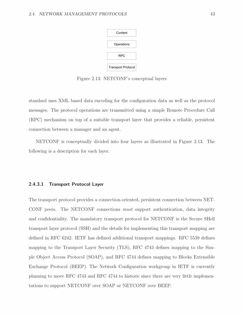
2.4. NETWORK MANAGEMENT PROTOCOLS 43
Transport Protocol
RPC
Operations
Content
Figure 2.13: NETCONF’s conceptual layers
standard uses XML based data encoding for the configuration data as well as the protocol
messages. The protocol operations are transmitted using a simple Remote Procedure Call
(RPC) mechanism on top of a suitable transport layer that provides a reliable, persistent
connection between a manager and an agent.
NETCONF is conceptually divided into four layers as illustrated in Figure 2.13. The
following is a description for each layer.
2.4.3.1 Transport Protocol Layer
The transport protocol provides a connection-oriented, persistent connection between NET-
CONF peers. The NETCONF connections must support authentication, data integrity
and confidentiality. The mandatory transport protocol for NETCONF is the Secure SHell
transport layer protocol (SSH) and the details for implementing this transport mapping are
defined in RFC 6242. IETF has defined additional transport mappings. RFC 5539 defines
mapping to the Transport Layer Security (TLS), RFC 4743 defines mapping to the Sim-
ple Object Access Protocol (SOAP), and RFC 4744 defines mapping to Blocks Extensible
Exchange Protocol (BEEP). The Network Configuration workgroup in IETF is currently
planning to move RFC 4743 and RFC 4744 to historic since there are very little implemen-
tations to support NETCONF over SOAP or NETCONF over BEEP.
44 CHAPTER 2. BACKGROUND AND LITERATURE REVIEW
2.4.3.2 RPC Layer
RPC layer describes in detail the format of NETCONF messages. A NETCONF request
uses the <rpc> element to encapsulate a NETCONF operation. A NETCONF response uses
the <rpc-reply> element to encapsulate the reply message. <rpc-error> is sent as part of
<rpc-reply>message to indicate an error occurs during the processing of NETCONF request
message. The error message may include further elements to provide detailed description of
the error.
2.4.3.3 Operations Layer
NETCONF standard has defined a set of pre-defined operations to be used by a manager
to manage and control managed devices. In addition, the standard allows user-defined
operations to be included. In this case, a managed device must advertise these non-standard
operations as part of the device capabilities. All operations defined in the current version
of NETCONF are used by a manager.
NETCONF protocol distinguishes between two classes of management information: con-
figuration data and state data. Configuration data is the set of variables that can be modified
to configure a managed device. State data is the set of values that can be only read such as
status information and collected statistics. In addition, NETCONF distinguishes between
three repositories on a managed device: running, candidate and startup. Running reposi-
tory stores the current active configuration data. Candidate repository stores the standby
configuration. Startup repository stores the initial configuration of a device.
The base operations defined by NETCONF are:
• get: retrieve all or part of the current running configuration (running repository).
• get-config: retrieve all or part of a specified repository such as running or candidate.
• edit-config: create or modify all or part of a specified repository based on a set of
attribute operations. NETCONF defines the following attribute operations: merge,

2.4. NETWORK MANAGEMENT PROTOCOLS 45
replace, create, and delete.
• copy-config: copy the entire configuration data from a source repository to a target
repository.
• delete-config: delete the entire configuration data from a specified repository.
• lock: lock a given repository. This operation allows a manager to lock a configuration
repository so that no other managers can perform updates on the same configuration
repository.
• unlock: unlock a given repository.
• close-session: close an existing NETCONF session. Before a manager sends NET-
CONF operation, he/she establishes a session be sending HELLO. Sessions are iden-
tified by session id’s. A session will be kept open until the manager close or kill the
session.
• kill-session: kill an existing NETCONF session.
2.4.3.4 Content Layer
A new data modeling language called YANG has been developed specifically for NETCONF
protocol. YANG is standardized and published in RFC 6020. It is not an object-oriented
language but rather a tree-structured language. In other words, the management information
is structured as an inverted tree such that the leaves constitute the configuration and state
data.
In YANG, Management information is partitioned into modules where each module con-
tains one or more tree containers. A node in the tree may represent a simple data type such
as integer or a complex data type such as list or union. YANG has strong support for seman-
tic validation than other data model languages (such as SMI). In addition, a YANG module
can augment a tree in another module. This makes YANG very flexible for re-usability.

46 CHAPTER 2. BACKGROUND AND LITERATURE REVIEW
The advantages of using YANG for data definition include [87]:
• It is simple, easy to learn, and easy to read and understand.
• It is a domain specific language designed specifically for network management.
• It is flexible and modular. Existing modules can be augmented in a controlled manner.
2.4.4 Discussion and Critique
Although the CMIS/CMIP protocol suite has the capability of performing many manage-
ment tasks, there are two serious problems associated with the protocol suite. First, there is
a large amount of overhead to send/receive CMIS request/response. Second, CMIS/CMIP
lacks industry support. It requires full implementation of OSI protocol stack. As a result,
implementing CMIS/CMIP protocol is complex and costly. Moreover, network devices may
not have enough processing power or memory space to support full OSI protocol stack.
SNMP protocol has been widely accepted by both equipment vendors and network man-
agement systems. Even though SNMP is a lightweight protocol and provides operation to
configure network devices, it is only limited to collect statistics and status information from
network devices. It is rarely used for configuration purposes. There are several reasons for
this deficiency. Here, we mention the important ones:
1. SNMP protocol is simple, leaving the onus of manipulating configuration data on
the management application. For this reason, tool development based on SNMP is
expensive [76].
2. SNMP protocol stack has limited operational commands which are inadequate for large
heterogeneous networks [76].
3. SET requests are sent independently. This may cause a serious network problem if a
manager sent several SET requests to configure a particular device and one request is
failed.

2.4. NETWORK MANAGEMENT PROTOCOLS 47
4. SET request may contain a list of variable bindings. If one variable binding is not
valid, the whole SET operation will not be accepted.
5. SNMP does not provide any mechanism to undo recent changes in the device config-
uration.
6. SNMP does not provide synchronization among multiple network devices. If a manager
sends SET request to a group of devices (to have similar configuration), some of them
can succeed and others can fail.
7. SNMP does not employ the standard security mechanism. Instead, the security is
self-contained within the protocol itself, which makes SNMP credentials and key man-
agement complex and difficult to integrate with other existing credential and key
management systems.
NETCONF protocol has been developed to overcome the shortcoming of SNMP. One
of the major advantages of NETCONF over SNMP is how the protocol works when ma-
nipulating a group of semantically related configuration data. Whereas SNMP modifies the
value of a single parameter at a time, NETCONF modifies all or selected parameters on a
single primitive operation. Another advantage of NETCONF is that it allows configuration
to occur in a transactional manner. NETCONF takes into account when some of network
devices successfully uploaded the configuration, but others failed to upload the configura-
tion. NETCONF allows a managed device to rollback to a known-state configuration. This
is because NETCONF defines transactional model that synchronize, validate, and commit
device configuration within an entire network deployment.
Among the set of configuration standards described above, the most promising protocol
is NETCONF, which is expected to be widely accepted by many network vendors. Major
vendors of networking equipment are already started to implement the NETCONF standards
(version 1.0 and version 1.1) in their production. There is no standard framework for
NETCONF, but so far the framework consists of NETCONF protocol and the data modeling
48 CHAPTER 2. BACKGROUND AND LITERATURE REVIEW
language: YANG. The framework focuses primarily on the interaction pattern between a
manager and an agent, and YANG language provides the uniformity of data representation.
However, the framework cannot establish a bridge between high-level service configuration
requirements and low-level configuration data to support network-wide configuration. Our
contribution in this dissertation is to build such a bridge by defining a semantic model that
supports network-wide configuration.
2.5 Current approaches to network Configuration
Network configuration management has been evolved since commercial networks first ap-
peared. This section focuses on the protocol used to communicate with network devices in
order to access configuration data.
2.5.1 Manual configuration
In manual configuration, network administrators use Command-Line Interface (CLI) to man-
age their networks. They use SSH protocol, TELNET protocol or terminal servers to com-
municate to network devices [100]. Manual configuration is only feasible for small-sized
networks, but can be utilized for large networks in which few changes are expected over
time. The main advantage of CLI is that network devices are closely monitored during
each step of configuration. However, there are several disadvantages on using CLI. First,
network administrators can easily commit errors during configuration process. Second, in
multi-vendor networks, network administrators must remember all syntaxes and sequences
to configure network services. This becomes specifically tedious work when the network sup-
ports multiple and complex services. Finally, CLI is not scalable for large-sized networks.

2.5. CURRENT APPROACHES TO NETWORK CONFIGURATION 49
2.5.2 Script-based and template-based configuration
Script-based approach is considered the first step towards automation. In script-based con-
figuration, a sequence of commands is programmed in a script file, when executed it generates
a device-native configuration file (or commands) that can be directly uploaded to the device.
This approach is especially useful for automating a repetitive management task. The script
files are usually written using hybrid language; high-level language such as Unix shell, Perl,
Python or domain-specific language and a low-level language which describes the actual CLI
commands that an operator performs when configuring a network service or device.
Over the years, researchers have invested considerable efforts to improve script-based
approach. Here, we classify script-based approaches into three categories: customized script-
based approach, controlled script-based approach, and structured script-based approach.
In customized script-based approach [75], CLI commands or configuration files are en-
coded into modules or templates with placeholders for some key values instead of the actual
values. When a script file is executed, the placeholders are replaced with the values provided
as arguments. The main weakness of this approach is that CLI’s commands are sent blindly.
As a result, if a problem arises or an error occurs, continuing to send commands may not
have the intended effect.
In controlled script-based approach [10, 12, 69], the flow of execution is controlled based
on the execution behavior. The script language allows a manager to provide postconditions
based on the response it receives to handle unusual conditions.
Structured scripting (or template) is an enhancement of controlled scripting that allows
one to create scripts that are reusable on a larger network by providing a framework that
assures coordination between network devices that support a specific network service.
The work in [26], which has developed a management system called PRESTO to manage
large-scale networks, is one example of structured scripting. PRESTO generates device-
native configuration files based on a set of templates called configlets. Configlets are written
using a hybrid script language. The low-level language describes the actual commands that
50 CHAPTER 2. BACKGROUND AND LITERATURE REVIEW
an operator performs when configuring a network device, but without specifying configura-
tion values. The high-level language is used to extract the necessary information from ex-
ternal database to determine which devices involved in service configuration, and to provide
Configlets with the necessary configuration properties to produce complete configuration
file.
It is quite obvious that Configlet is device-specific template since the actual configuration
language is written using the device-native language. The work is suitable if the underlying
devices are homogeneous. However, the system becomes very complex for multi-vendor
networks since we need multiple Configlets for a single service.
Similar to PRESTO management system is NCG [68]. NCG is a management system
developed by the network operator community in North America. The system is still under
beta version. However, the idea of this system is quite similar to our idea on how to reduce
the network configuration complexity. NCG needs two inputs: network description and
NCG-based templates for the various configuration files of various devices. It generates, as
an output, the actual configuration for each device to be installed. Thus, NCG requires
manual pushing the configuration to network devices. AutoConf seamlessly integrates the
generation of configuration and pushing it to network devices using NETCONF protocol.
2.5.3 Vendor-neutral Configuration
To resolve the issue of script-based approach specially in heterogeneous environment, man-
agement system must communicate with the underlying devices using vendor-neutral lan-
guage.
SNMP-based configuration is one solution that provides vendor-neutral configuration [72,
67]. Due to the limitation of SNMP, many industrial tools, such as [61, 77] combine SNMP-
based configuration with script-based configuration.
HTTP-based approach uses HyperText Transfer Protocol (HTTP) to transfer manage-
ment information between agents and managers. In this case, agents (which are usually

2.5. CURRENT APPROACHES TO NETWORK CONFIGURATION 51
referred as web-based agents) must have HTTP-server embedded in order to support HTTP-
based configuration. Managers are simply web browsers.
The web-based agents may send static web pages to the managers or dynamic web pages,
both encoded in HyperText Markup Language (HTML) [64]. Java applets and Servlets are
also common methods of interactions in which HTTP is used to communicate between the
manager and the web-based agent [9, 62].
A number of vendors have been working on XML-based management for several years.
Juniper Networks developed Junos XML API for the Junos network operating system [51].
This API gives management applications full access to the agent’s management information
using Junos XML management protocol [52], which was formally known as JUNOScript.
In addition to Junos XML framework, Juniper networks as well as Cisco started to adopt
NETCONF protocol in their devices.
Many academic research projects have been proposed for XML–based network manage-
ment systems. The work in [58] developed a software system called Netopeer to configure
IP routers. Ju et al proposes an XML-based management architecture that is based on
XML/HTTP as its management protocol [50]. The work in [63, 99, 21] focused on the
translation of SNMP MIB modules into XML document. Other work [30, 5] focused on
implementing SNMP/XML gateway.
2.5.4 Declarative-based Configuration
The increasing complexity along with administrator errors points towards an inevitable need
to automate network configuration management. To handle rapidly growing complexity
and to enable further growth, many approaches adopt the use of high–level programming
language to describe the network behaviors. The main objective is to automate network
management and reduce human involvement.
The literature comprises several works on providing automation in network configura-
tion management. In addition, plethora of research work exists on autonomic computing
52 CHAPTER 2. BACKGROUND AND LITERATURE REVIEW
concept which provides autonomic computing for system management [82, 49]. Here, we
only summarize the work related to automate configuration management.
SmartFrog [32] is framework for service configuration, documentation, deployment, and
life-cycle management. The basic idea of SmartFrog framework is to visualize services as
set of components. The component model enforces life-cycle management by transitioning
components into five states: installed, initiated, started, terminated and failed. The frame-
work comprises of an object-oriented language that supports encapsulation and inheritance.
The language allows customized composition of service configuration by support post- and
pre-conditions. The language enables static and dynamic bindings between components to
support different ways of connecting components at deployment time. In addition, it has its
own data model specification.
The work of Narain [66] proposed a solution to automate network configuration man-
agement tasks by formalizing high-level requirements using first-order predicate logic. The
basic idea is to describe the network logically. Then, a requirement solver, which is basically
a Satisfiability (SAT) solver, takes the description and tries to find a set of values that satisfy
the logic. The work uses Alloy system as “requirement solver” system.
The network specification is written using the Alloy language, and it consists of three
parts: components declarations which follow object-oriented paradigm, a set of predicate
specifications (requirements), and model parameters. Alloy takes as input the network
specification and produces components configurations satisfying those requirements.
The work is suitable for network design problems where it provides high-level description
of network configuration. There are two major limitations in this work. First, the resulted
configuration is described in a high-level language that requires an additional tool to translate
the high-level language into device configuration. Second, the network specification will be
too complex for large-scale networks, and network administrators may encounter difficulty
to write efficient requirements. As a result, the SAT solver may not be able to produce an
output at all.
2.5. CURRENT APPROACHES TO NETWORK CONFIGURATION 53
2.5.5 Policy-based approach
Policy-based management (PBM) has become a promising solution for managing networked
systems. The main motivation of PBM is to reduce the human intervention by providing
dynamic adaptability of behavior by reconfiguration and addition of new policies without
harming network operation [14]. This implies that PBM system should (i) transform man-
agement requirements to syntactical and verifiable rules governing the function and status of
the network, (ii) transform such policy rules to device-native configuration, and (iii) enforce
these configurations to managed devices.
One of the first architecture for self-managed networks introduced in literature called
NESTOR [98]. NESTOR is organized in a four-layer architecture. The first and second
layers (the bottom layers) emphasize the role of a uniform object-relationship model of
network resources, in order to allow any kind of manager (human or software) to configure
and control the network behavior. The network resources are expressed by using Resource
Definition Language (RDL). RDL is an object-oriented interface language that supports
the specification of resources as objects and their relationships. The top layers emphasize
the role of uniform traditional interactions with the underlying resources. This is achieved
by defining a shared object repository that unifies transactions and constraints that can
be imposed to prevent known configuration inconsistencies. A language called Constraint
Definition Language (CDL) is used to express the modeler constraints.
The IETF started its efforts by describing the architecture of PBM, which consists of
Policy Decision Points (PDP), Policy Enforcement Point (PEP), Policy repository and Pol-
icy management tool defined in RFC 3198. Policies are defined through Policy Management
Tools and those policies are stored in Policy Repository. PDP is responsible to take decision
based on policies stored in Policy repository. PEP is responsible to enforce the decisions
on managed devices. PDP and PEP are communicated through a protocol called Common
Open Policy Service (COPS), which is defined and published in [4]. In PBM, policy in-
formation is represented through the Policy Core Information Model (PCIM), which is an

54 CHAPTER 2. BACKGROUND AND LITERATURE REVIEW
extension to DMTF’s CIM model, and PCIM was produced jointly by DMTF and IETF
(see [65]).
Sloman and Lupu [78] provide a comprehensive, but slightly outdated, description of
management policy specification. One of the key points they raised is that there is a marked
separation between policy languages that are applied to specific domains. The authors
along with others have developed a policy language called Ponder as part of ongoing work
in Imperial College, London [24]. The authors distinguish six types of policies: positive
authorization, negative authorization, refrain, positive delegation, negative delegation and
obligation. The Ponder language is declarative object-oriented language that supports these
policy types. While these policy types allow for a rich policy set for management, it has
some shortcomings. Refrain, positive authorization and negative authorization policies have
no event clause, which can cause efficiency and predictability problems.
The work in [83] proposed a tool called Focale that uses PBM to automate network
management. It uses ontologies to model the managed resources and heterogeneous data by
mapping their facts into a common vocabulary. Focale uses a mid-level model called Model-
Based Transaction Layer to convert high-level policies into device-native configuration data.
The developers of Focale have introduced the term “Policy Continuum” to indicate that a
policy may be viewed on different constituencies. This means that a policy can be placed
on different abstraction levels.
2.5.6 Separating Data and Control planes approaches
Several research works have addressed the network management complexity by raising two
key points: (1) separating the functionality of the data plane and control plane and (2)
programmability instead of configuration [73, 56]. This has led to a new paradigm named
software defined networking (SDN).
The grandfather of SDN is 4D project [34], which has addressed the need for sepa-
rating between control and data planes as well as centralized administrative domain. 4D
2.5. CURRENT APPROACHES TO NETWORK CONFIGURATION 55
architecture actually proposed four planes: decision plane, dissemination plane, discovery
plane, and data plane. The decision plane determines the overall network behavior based
on network-wide view collected from the underline devices. The data plane performs ba-
sic packet processing functions such as forwarding, filtering, etc. The dissemination plane
serves as a communication mechanism between the decision plane and data plane. The dis-
covery plane is responsible for discovering the underlying physical devices. The concept of
4D concept has been implemented in Tesseract system [97]. The system has been designed
to provide a platform with pluggable programmable modules.
CONMan [8] architecture defines a set of abstract modules that capture data or control
plane functions. Ethane [16], NOX [35], and Maestro [97], which are all inspired by 4D
project, are focusing on network flow access control management. Ethane has been deployed
at Stanford’s Computer Science Department, which gave the developers a real evaluation to
the concept of 4D.
The success of Ethane has led to OpenFlow, an open standard for programmable flow-
based switch developed by Open Networking Foundation [71]. An OpenFlow-capable switch
processes packets according to a flow table. The flow table is a set of matching rules over
packet headers such that each rule has an action to be taken. A “logically” centralized
controller is responsible to control the flow tables in OpenFlow capable switches using a set
of pluggable, programmable modules.
Currently, SDN paradigm is a popular programmable architecture. It allows administra-
tors to program their network and to deploy network services via programmability instead
of configuration. on the other hand, our work is focusing on network configuration manage-
ment.
2.5.7 Discussion and Critique
We presented various techniques to automate network configuration management. Majority
of these techniques rely on a high-level language where the language has its own data type
56 CHAPTER 2. BACKGROUND AND LITERATURE REVIEW
definitions. This may create a conflict between the data type of a specific configuration
parameter defined in the language and the data type defined at the device level. Moreover,
if network devices are managed via standard protocol like SNMP, the overall management
architecture will end up with two different data models: a data model at higher level (part of
high-level language) and a data model provided by the standard protocol (such as YANG or
SMI). Our approach provides automation by using programming and policy based approach;
however, the language is designed to orchestrate with the data modeling language. Thus,
instead of having a single complex model to translate high level policies into device native
language (as in FOCALE and SmartFrog), our proposed framework divides management
complexity into a set of layers where the lower layers are based on a standard architecture
which is the NETCONF framework.
We mentioned various approaches that define the interaction protocol between a manager
and an agent in order to manage configuration data. A manager can access the configu-
ration data either directly or indirectly. A direct access is achieved by using CLI through
manual configuration or script-based configuration. These approaches have the advantage
of efficiency since they do not require a translator (to translate from high-level language to
device-native language). The disadvantage is that each device may have its own language or
CLI. Using manual configuration and script-based configuration in a heterogeneous network
are impractical.
Indirect access is achieved by having a high-level language and a management protocol.
It requires a translator application (agent application) to translate high-level language to
device-native language. The purpose of having a high level language is to have a unified view
of related configuration data regardless of the device manufacturer. SNMP-based approach
is considered the most dominant approach to access configuration data indirectly due to its
simplicity and low cost. Before SNMP-based approach, the object-based approach existed
but was not widely accepted due to the extra overhead when transferring managed objects.
With advent of Internet, HTTP-based approach has been introduced. HTTP-based

2.6. CONFIGURATION VERIFICATION APPROACHES 57
configuration has the same advantage as in SNMP-based approach. However, it has the
same disadvantages as in the script-based approach.
XML-based approach is considered the most attractive technique to access configuration
data due to the powerful features of XML technology. The work in this dissertation uses
XML-based approach since we rely on NETCONF protocol to convey configuration data.
As reported by [100], the downside of XML is overhead when handling with a single value
of configuration data.
Recent approaches to automating network configuration management are influenced from
software engineering principles. The main shortcoming in these approaches is the device
life cycle, which is based on an isolated computer system life cycle [89]. However, our
approach concerns about the life cycle of a whole network in order to achieve network-wide
configuration.
Our work is not much different from the concept of SDN even though our work focuses
on traditional network management. OpenFlow-enabled network can still benefit from our
work in two areas: the bootstrapping of the network and policy manipulation. Based on [71],
OpenFlow-enabled network is relying on NETCONF protocol as a main protocol to configure
switches and controllers during the bootstrapping. Moreover, the work in this dissertation
provides a solution to manipulate and verify flow tables.
2.6 Configuration Verification Approaches
In the past few years, many researchers have attempted to address various challenges in net-
work configuration management, and most of which have focused on detecting configuration
conflicts within certain devices. The work in [36, 101, 33] focused on firewall devices. The
work in [29] [90] focused on detecting routing misconfiguration.
Static, end-to-end formal analysis was first introduced by [94] and later has been extended
and implemented by [55]. Our work is similar to their work with some differences. Our
58 CHAPTER 2. BACKGROUND AND LITERATURE REVIEW
approach models a network as a graph over links, while [94] and [55] model a network over
devices. There are two advantages using our graph model. First, it allows us to provide
fine-grained analysis since we encode the effect of each device on its incident links. Second,
their algorithm runs in O(|V |3) time ignoring the cost of set operations, where V is the
number of vertices (devices) in a graph. Our algorithm in worst case runs in O(2 × |L|2)
time, where L is the number of links in a network. Moreover, in [55], the paper assumes
that any packet passing a NAT device will be translated but the translation function is not
well defined.
Global verification has also been discussed in [1]. The authors have used model checking
to achieve end-to-end analysis. The main disadvantage is that the model formalization uses
huge number of bits (591 bits). In addition, using BDD representation for model checking
has the limitation of the state-explosion problem, particularly when used to verify large
networks.
2.7 Summary
This chapter started with a brief introduction to the methodologies and models that will
be used in this dissertation. Then, we presented the major contribution of standard bodies
in network configuration management and the major network configuration protocols. We
analyzed the prior work for network configuration management by dividing it into three
dimensions. The first dimension concerns on how to access the configuration data. We
presented several approaches starting from manual configuration up to XML-based con-
figuration. The second dimension concerns on configuration management scalability. We
presented several prior projects along with their limitations. The third dimension concerns
on automating network configuration. We presented different approaches to achieving au-
tomation using policy-based techniques. We concluded this chapter by reviewing recent
research works in configuration verification.
Chapter 3
Configuration Semantic Model
Management systems require a detailed description of managed devices and their associ-
ated services to automate network configuration. This chapter provides an overview of
required functionalities of an automated system. Then we describe the main components
of our proposed system: AutoConf. Moreover, we introduce an information model called
Configuration Semantic Model (CSM) along with its associated language called Structured
Configuration Language (SCL). Then we show how CSM and SCL simplify configuration
process by abstracting away the underlying complexity of configuration process.
3.1 Overview
Given the complexities and challenges of network configuration, an effective configuration
framework does not only define a model to unify all data but also provide a global view of
all knowledge needed to support automated network management.
Recent approaches to automating network configuration management are influenced from
software engineering principles. The main shortcoming in these approaches is that they rely
on the concept of device life cycle, which is based on an isolated computer system life
cycle [89]. The purpose of studying device’s life cycle is to ensure a flawless operation of
59

60 CHAPTER 3. CONFIGURATION SEMANTIC MODEL
Planning Implementation
OperationUpgrading
Termination
Figure 3.1: Life cycle of a networked device
networked system. Based on software engineering, the life cycle comprises of four stages:
planning, implementation, operation, upgrade and termination as shown in Figure 3.1.
However, a healthy network has a set of services (or functions) operating in a harmonic
way. A network service is not only associated with a single device. For example, OSPF
routing protocol is meaningless with a single network device. Furthermore, a network service,
when operates, should not harm other network services. Thus, a life cycle, which ensures
flawless operation of a networked system, must capture the network as a whole not as an
individual device or service.
Our envision for an efficient automated network configuration is based on the following
features:
• The automated system should support standard technologies. This will guarantee the
ability to manage the same network services independently of the underlying network
device’s hardware or operating system.
• The system should scale well, so distribution of management activities on the local
management domain has to be attained.
• The system should be able to automatically configure and continuously validate all rel-
evant network services in the management domain. The configuration is accomplished
based on a set of policies that define administrator’s requirements.
• An independent high-level specification language should be adopted to configure all

3.2. THE FRAMEWORK 61
Network Resource
Discovery
Change
ManagementNETCONF
protocol
AutoConf Management System
Monitoring
Protocol(s)
Dynamic
Management
FAPS
management
Network Resources
Validation
Management
Figure 3.2: AutoConf management system
network services, network devices and the management system itself. This language
forms a unified interface between a network administrator and the automated system
that allows administrators to access all underlying devices and to define requirement
specifications.
3.2 The framework
The problem of network configuration management is divided into three parts. The first part
explores the configuration change management. The focus of this part is to improve con-
figuration management by organizing management functions semantically and formalizing
configuration specifications. The second part focuses on configuration validation manage-
ment. This part explores the theoretical approach to validate network configuration as well
as network behavior. The third part concerns on dynamic network configuration, which is
responsible for responding to any change in network state. The response should take into
consideration the high level requirements stated by network administrators and the current
network state.
Figure 3.2 shows the overall components of our proposed automated management sys-
tem called AutoConf. AutoConf system relies on NETCONF protocol to query or change
the configuration of network resources. Network Resource Discovery uses NETCONF and

62 CHAPTER 3. CONFIGURATION SEMANTIC MODEL
YANG to define the set of resources that need to be managed and controlled within the
domain environment. Once the resources are defined, AutoConf system goes through two
cycles. Both cycles start at the change management. The change management is either
triggered automatically or manually, which adds, deletes, and updates configuration data
of network resources. The validation management will automatically be triggered to read
operational data and report the result back to the automated system. This will constitute
the first cycle. The Fault, Accounting, Performance and Security (FAPS) management will
continuously monitor the network resources. Any deviation from normal state will be re-
ported to the dynamic management. The dynamic management analyzes the report and
informs its decision that should be taken to correct the situation to AutoConf system. This
will constitute the second cycle. The automated system invokes the change management to
enforce the new change automatically and hence the first cycle will be performed.
The aforementioned parts are not isolated but rather orchestrated by a common frame-
work as shown in Figure 3.3. The framework assumes that managed resources are running
NETCONF servers (netconfd). Netconfd acts as an agent and translates NETCONF mes-
sages into device-native management information and vice versa. If a network device does
not support NETCONF, a proxy NETCONF server will be used.
The framework supports distributed management framework with a centralized database
management. Remote managers write SCL commands to manage and control network
services and resources. SCL engine, which is part of AutoConf engines, translates SCL
commands and generates NETCONF messages to be sent out via NETCONF protocol to
netconfd servers. SCL engine and Netconfd servers must follow YANG specifications to
exchange management information1. In addition to SCL commands, Remote managers
describe their intentions or requirements by using the CSM, which covers the required infor-
mation to automate configuration management. In the following sections, we describe the
semantic model and the SCL specification.
1The YANG language is explained in Appendix A

3.3. CONFIGURATION SEMANTIC MODEL CONCEPTS 63
Remote
manager
Remote
manager
Network
Topology
Information
Configuration
Specification
Configuration Semantic Model (CSM)
AutoConf Engines
NETCONF Layer
YANG data model
Netconfd Netconfd Netconfd Netconfd
MIB MIB MIB MIB
Remote
manager
Device-native management information
Managed objects
Agent Application
Policy
specification
Manager Application
Management Protocol
High level requirements
Figure 3.3: AutoConf framework
3.3 Configuration Semantic Model Concepts
To improve the configuration process and change management, a middle level is required
to link the dependencies between configuration information and to allow network admin-
istrators to enforce certain policy and consistency rules on configuration data that resides
on different network devices. In other words, the main purpose of the semantic model is to
engineer and manage the high-level knowledge about the network, management functions,
network services and the underlying devices. We call this semantic layer Configuration
Semantic Model (CSM).

64 CHAPTER 3. CONFIGURATION SEMANTIC MODEL
The main objectives of having configuration semantic model are two-fold. The first
objective is to interlink configuration semantics to establish network-wide configuration.
The second objective is that CSM abstracts away the details of individual configuration
data and instead works on a unified abstraction, which fundamentally establish a common
vocabulary between the Automated System and network administrators.
Our methodology to construct CSM model is to use knowledge management engineering
as described in [53]. CSM model has a set of concepts. A concept, which represents an
ontology in the domain of network management, is characterized by a set of attributes and
possible classification. Thus, concepts are organized in hierarchical format and stored in a
centralized database such that multiple managers can access the same database.
Generally, CSM covers four types of information: topology specifications, configuration
specifications, policy specifications and status specifications. The following sections define
the set of CSM concepts (or ontologies) that are used to describe each information.
3.3.1 Topology Specification
Network topology is modeled by using the following concepts: device, service, interface,
link, data, yang, and repo. The following is a description for each one:
Device: This concept provides a logical representation of any network element that needs
to be controlled and managed. It is not necessarily representing a physical device; a device
can be a logical element such as an autonomous system or a management domain. A device
is characterized by a name, a parent device, and a group. A device may have one or more
children devices. In this case, the device represents a domain. A domain device semantically
links several devices to form a logical domain. Configuring these devices can be accomplished
by configuring the domain device. For example, let us consider a network with three routers
that run OSPF routing protocol. Instead of configuring each device individually, we may
create a domain device and configure that device only.
3.3. CONFIGURATION SEMANTIC MODEL CONCEPTS 65
Interface: This concept represents an abstraction of an interface. An interface can be a
logical interface or a physical interface. It is a part of a device resource. An interface is
characterized by a name, a device name, an index number, and info. The attribute info is a
list of properties for describing the interface.
Link: Link is an abstraction for any type of connectivity between two adjacent devices.
CSM allows to build a hierarchy of connectivity between two adjacent devices. For example,
router A is physically connected to router B using 1000Base-T Ethernet cable. The routing
table of router A indicates that router B can be its next hop. Thus, router A and router
B are logically connected. However, the logical connectivity cannot be exist unless there
is a physical connectivity between the two routers. To express this scenario, CSM allows
us to define a link where its existence relies on the existence of its parent link. link is
characterized by a class, ports, and a parent link. If a link has no parent, then parent link
is undefined. Ports is a list of two tuples such that each tuple represents an end point. For
example, {link, fa, undefined, [{r1, 1}, {r2, 1}]}.
Service: The concept of service abstracts any activity (at any OSI layer) that needs to
be managed. A service is characterized by a name and a group of activities. For example,
OSPF is a service that performs routing activity.
Data: Each service is associated with one or more data modules that determine its behav-
ior. One reason of having multiple data modules for a single service is to provide multiple
views for the same network service. For example, it is possible that a network accommodates
two routers from different vendors. Both routers support OSPF protocol; however, each has
its own data representation. As such, the service OSPF has two data modules.
A data is characterized by a service name, data type, and module name. Data type is
the data model used such as YANG or SNMP SMI.
66 CHAPTER 3. CONFIGURATION SEMANTIC MODEL
Yang: If a service has a data module of type YANG, there will be a concept of type yang.
A yang concept is characterized by module name, prefix, namespace, list of container names,
and YIN root. YIN is the equivalent representation of YANG module in XML format.
Repo: A device may have several data repositories. When a manager needs to configure
a network device, it accesses a specific data repository of that device and starts modifying
its data. A repo is characterized by a device name, data module type, data module name,
data module info, and options.
To illustrate the relationship between the above concepts, let us consider a border router
called RTR01 in area one that supports multiple routing protocols such as RIP, OSPF
and BGP. We describe the topology as follows. The network devices are area-one and
rtr01 where area-one is the parent device of rtr01. We classify rtr01 as router and
border router. The network services are rip, ospf, and bgp; all doing routing activity.
Assuming the network supports NETCONF and YANG. Each service is associated with a
data module of type YANG. rtr01 supports the following repositories: ospf data module,
rip data module, and bgp data module.
AutoConf system creates repositories automatically by navigating device capabilities.
However, a network administrator must manually define services and data modules. The
reason is to give more controls at the manager side what configurations are required. In other
words, defining services and data modules specifies AutoConf capabilities. For instance, a
router may support many intradomain routing protocols such as RIP, OSPF, IGRP, and
ISIS. We may only tell AutoConf to consider OSPF and RIP when automating routing
activity.
3.3.2 Configuration Specification
The CSM allows a domain expert to extend its model by introducing user–defined ontologies.
These ontologies are intended to provide a unified view of the current network configuration.
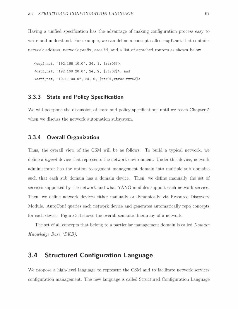
3.4. STRUCTURED CONFIGURATION LANGUAGE 67
Having a unified specification has the advantage of making configuration process easy to
write and understand. For example, we can define a concept called ospf net that contains
network address, network prefix, area id, and a list of attached routers as shown below.
<ospf_net, "192.168.10.0", 24, 1, [rtr03]>,
<ospf_net, "192.168.20.0", 24, 2, [rtr02]>, and
<ospf_net, "10.1.100.0", 24, 0, [rtr01,rtr02,rtr03]>
3.3.3 State and Policy Specification
We will postpone the discussion of state and policy specifications until we reach Chapter 5
when we discuss the network automation subsystem.
3.3.4 Overall Organization
Thus, the overall view of the CSM will be as follows. To build a typical network, we
define a logical device that represents the network environment. Under this device, network
administrator has the option to segment management domain into multiple sub domains
such that each sub domain has a domain device. Then, we define manually the set of
services supported by the network and what YANG modules support each network service.
Then, we define network devices either manually or dynamically via Resource Discovery
Module. AutoConf queries each network device and generates automatically repo concepts
for each device. Figure 3.4 shows the overall semantic hierarchy of a network.
The set of all concepts that belong to a particular management domain is called Domain
Knowledge Base (DKB).
3.4 Structured Configuration Language
We propose a high-level language to represent the CSM and to facilitate network services
configuration management. The new language is called Structured Configuration Language

68 CHAPTER 3. CONFIGURATION SEMANTIC MODEL
Network
device
Domain
device
Domain
device
Element
device
Element
device
Element
device
Element
device
device
service
interface
data
Figure 3.4: The hierarchical structure of Configuration Specification
(SCL). It consists of a set of instructions aimed to create, view, manipulate, and delete data
stored in configuration repositories as well as to manipulate CSM concepts. The language
has the following features:
• Simple and easy to read. The language contains small set of statements and rich set
of useful functions. The syntax of SCL is very close to the syntax of YANG modeling
language. Therefore, it would not be difficult for an administrator to read and write
SCL code as well as YANG modules.
• Conform to NETCONF framework. Unlike other languages2, SCL is a tree-
structured language which makes it suitable for NETCONF protocol and YNAG lan-
guage. The reader of SCL commands can see the high-level of configuration specifica-
tions while understanding how the operations will be encoded in NETCONF requests.
• Aggregation. A single SCL command can configure a group of networking elements
by sending multiple NETCONF messages.
• Atomicity. One important feature of the SCL is that it supports an atomic statement
which means SCL statement with atomic option enabled will either be executed com-
2Such as CIM Query language
3.4. STRUCTURED CONFIGURATION LANGUAGE 69
pletely or not at all. SCL assumes that NETCONF servers support rollback capability
in order to achieve atomicity.
For more details, the reader can refer to appendix B.
3.4.1 Improved Configuration Management
SCL statements that are responsible to manage network devices consist of a domain model
followed by one or more configuration rules. The separation between domain model and
configuration rules allows the manager to focus on service management regardless of the
underlying network devices. A domain model provides the set of devices we should deal
with. Configuration rules provide the actual configurations for managing a network service.
Each rule handles certain data model version. The mapping between a data model version
and a network device is achieved automatically by AutoConf.
AutoConf management system exchanges NETCONF HELLO message with each device
in the network. Through these messages, AutoConf discovers the capabilities of each network
device and what data model versions it supports. These capabilities are stored in KDB via
repository concept. Therefore, when AutoConf processes SCL statement, it will consult
device repositories to resolve the configuration rules.
The general syntax of SCL statements that manage network devices is:
domain : service_name [ constaint ]
configuration rules
A domain can be a single device (specified by device name), a group of devices (specified
as a list) or a parent device. A parent device is analogous to super class in object-oriented
paradigm. The constraint is pertaining to domain model that provides a fine-grained selec-
tion of network devices. Let us illustrate it by using an example.
Figure 3.5 shows a network with a set of routers. The shaded rectangles represent the
conceptual representation of these devices along with the network using CSM device concept.

70 CHAPTER 3. CONFIGURATION SEMANTIC MODEL
Conceptual
Representation of a
network
Conceptual
Representation of
device
Figure 3.5: A network with a set of edge and core routers
As we mentioned before, CSM allows us to conceptually represent a network as a logical
entity that encapsulates all network devices in the network. Here the network device acts
as a parent device of all router devices.
If we need to enable OSPF configuration on all routers in the network, then our domain
will be the network device itself. Configuring the network device is equivalent of configuring
all devices in the network. If a network operator is requested to enable specific QoS, then
he/she needs to perform some configurations at edge routers and core routers. If the target
devices are all edge routers then the domain will be the network device with a constraint that
devices should belong to edge router. Please refer to section 3.3 on how to define groups.
Configuration rule provides the actual configuration for a specific data model version. For
example, if a network operator needs to enable network interfaces in routers, but there are
different versions that describe network interface data model (e.g. YANG model developed
from Cisco vs. YANG model from Juniper), then he/she should provide a configuration
rule for each data model without concerning the underlying physical device. AutoConf
selects the rule that matches the device capability automatically. Therefore, CSM and SCL

3.5. SUMMARY 71
framework simplifies configuration process by shifting the focus from physical configuration
management to service management.
In Chapter 7 we show how CSM configuration specifications abstract away the low level
configurations.
3.5 Summary
Using configuration management language whose process is close to manual administration
simply does not work in large and heterogeneous networks with different data representations
for the network service. When enabling a network service in heterogeneous networks that
involves multiple devices, administrators face subtle configuration process. Indeed, the subtle
interactions between different versions of the same of network service can make the cost
of management process excessively large. As a result, we developed a new framework to
accommodate management activities and proposed a new information model called CSM
to provide high level of network configuration process. To enable CSM, we designed a
new language called SCL that significantly reduces the complexity of network configuration
management.

Chapter 4
Configuration Verification
4.1 Overview
Modern networks are designed and deployed to satisfy a wide variety of competing goals
related to different network requirements, such as security vs. availability, and performance
vs. manageability. These high–level goals are realized through a complex chain of config-
uration commands which include service provisioning configurations along with thousands
of access control rules from different policies such as packet filtering rules, routing policies,
and packet transformations.
Due to various reasons, including security policy updating, new service provisioning, and
system upgrading, network configuration needs be often revised accordingly, which makes
the probability of misconfiguration unfortunately high. As we mentioned in Chapter 1,
several surveys show that misconfiguration is the most critical threat to network operation.
In addition, a local configuration change or network failure may even inadvertently result
in a global impact on existing network services or policies. For example, when a network
link goes down, the network may converge into a new topology that has not been envisioned
by network administrators. This may indirectly cause illegitimate traffic bypass security
protection or legitimate packets accidentally blocked. Thus, verifying network configuration
73

74 CHAPTER 4. CONFIGURATION VERIFICATION
routinely based on dynamically updated (e.g., via SNMP trap) network topology is a highly
desirable network service to enhance network reliability and manageability.
It is a significant challenge to verify in a timely fashion the configurations of a network
system, which may consist of hundreds or thousands of different devices with possibly hun-
dreds or thousands of configuration rules on each device. Network debugging tools such as
traceroute or ping can test network reachability but cannot reveal the details of reachable
packets. There is a growing consensus on the need of formal models and programming inter-
faces to conduct configuration verification in order to validate enforced network policies. As
such, many researchers have proposed formal models of network security and reachability
such as static analysis [94], firewall decision diagram [33] and model checking [1] as a solution
to overcome the limitation of debugging tools.
However, the proposed solutions suffer from a serious limitation which always requires
a complete construction of the entire model in order to answer queries for checking various
service reachability and security polices. Enterprise network administrators and Internet
service providers, in case of any topology change or network failure events, require a timely
diagnosis to maintain their network integrity and service quality and to reduce potential
revenue loss.
In this chapter, we divide the problem of configuration verification into two main cat-
egories: Consistency verification and Behavioral verification. Within each category, we
further divide it into a set of scopes. We named these scopes configuration verification lev-
els. Therefore, under a category, we analyze the verification problem by breaking it into a
set of verification levels and propose a solution at that level.
4.2 Network Verification Levels
When we need to verify a network operation, we construct a set of verification rules such that
one or more rules are pertaining to a specific requirement or administrator’s intention. There
4.2. NETWORK VERIFICATION LEVELS 75
are different scopes (or levels) of network requirements. For example, one may specify the
following two requirements: certain traffic should not pass through a specific intermediate
device and there is a connectivity between two subnets. The first requirement is related
to a single device while the second one is related to a group of devices. Moreover, some
requirements should be specified to ensure the correct operation of a network. For examples,
we may need to verify that dependent configuration parameters are consistent, or we may
need to verify that for any two routers that are directly connected by a link, the two interfaces
attached to the link have IP addresses that belong to the same subnet. In this dissertation,
we propose the following levels to achieve network verification:
• Data-level verification, which is pertaining to the data uploaded to network devices,
• Device-level verification, which is pertaining to a network device,
• Link-level verification, which is pertaining to directly linked devices,
• Service-level verification, which is pertaining to a group of devices that are collaborat-
ing to achieve a specific network service, and
• Network-level verification, which is pertaining to some or all network device function-
alities to achieve high-level requirements such as reachability, security, etc.
Since there are two types of data in any network: configuration data and state data, we
distinguish two types of verification:
• Consistency verification, to check the consistency of configuration data at some spec-
ified levels
• Behavior verification, to ensure status information such as access control lists or rout-
ing tables on network devices are valid and do not conflict with high-level requirements.

76 CHAPTER 4. CONFIGURATION VERIFICATION
4.3 Consistency Verification
Network configuration may involve several devices in order to enable a network service. For
example, OSPF routing protocol requires all devices in a single network to enable OSPF
process. Otherwise, OSPF will not operate successfully. We distinguish several levels of
consistency verification: data–level, device–level, and service–level verifications. Data–level
verification concerns about the correctness of the uploaded configuration data in general.
For examples:
• Is an interface configured with a valid IP version 4 address?
• Given an interface name, does this name exist in the configured device?
Link–level verification concerns about the consistency of configuration data between two
devices that share a common link. For example, the IP addresses of any two linked interface
must be consistent. Device–level concerns about the consistency of configuration data that is
related to a single device. One example at this level is to ensure that no two distinct interfaces
of the same device are placed on the same subnet. Service–level verification concerns about
the correctness of configuration data to enable a network service. The OSPF example given
above demonstrates service–level verification. In this section, we discuss how to provide a
consistency verification at data, device, link and service levels.
4.3.1 Data–level Verification
At data level, we rely on YANG data model since YANG provides an efficient mechanism to
ensure the correctness of syntactic and semantic of configuration data. In addition, several
parameters can be logically compared using must with XPath expressions. must statement
is very useful when the existence or possible state of a parameter may depend on another
parameter that exists somewhere else in the same configuration data module.

4.3. CONSISTENCY VERIFICATION 77
4.3.2 Device and Service-level verification
When configuring a network service, we need to ensure the state of a parameter is consistent
with other states of the same parameter on other devices. For example, we need to ensure
that the OSPF timers on one router is consistent with OSPF timers on other routers that
provide OSPF service. To model this, let S be the set of states of a parameter on different
devices. Then the set S is consistent if the following verification rule is true:
Q x ∈ S : F (x) (4.1)
where F is a constraint over x, and Q is quantifier that can take values as tabulated in
Table 4.1. For example, all x : F (x) is true when each value in S satisfies F (x), and
-1 x : F (x) is true when at most one value of x satisfies F (x).
Q meaningall universal allsome existentialno no valuesN exactly N values+N at least N values−N at most N values
Table 4.1: Quantifier values
To construct a verification rule, we first need to specify the set S. In heterogeneous
network, not all services are modelled using the same data model; each service might be
modelled by using vendor-specific data schema. This means that the location of a configu-
ration parameter in one device may differ from other devices.
One possible solution is to use XML transformation or XSLT (Externsible Stylesheet
Language Transformations). XSLT is a set of rules that transforms an existing XML doc-
ument to a new XML document, as shown in Figure 4.1. The rule’s matching criteria in
XSLT is an XPath expression. When there is a pattern matching, the rule’s template form
will be evaluated, and the result constitutes XSLT processor’s output.
Writing XSLT for various devices to match vendor-independent schema could be a tedious
job. On one hand, network operators must learn how to write XSLT documents. On another
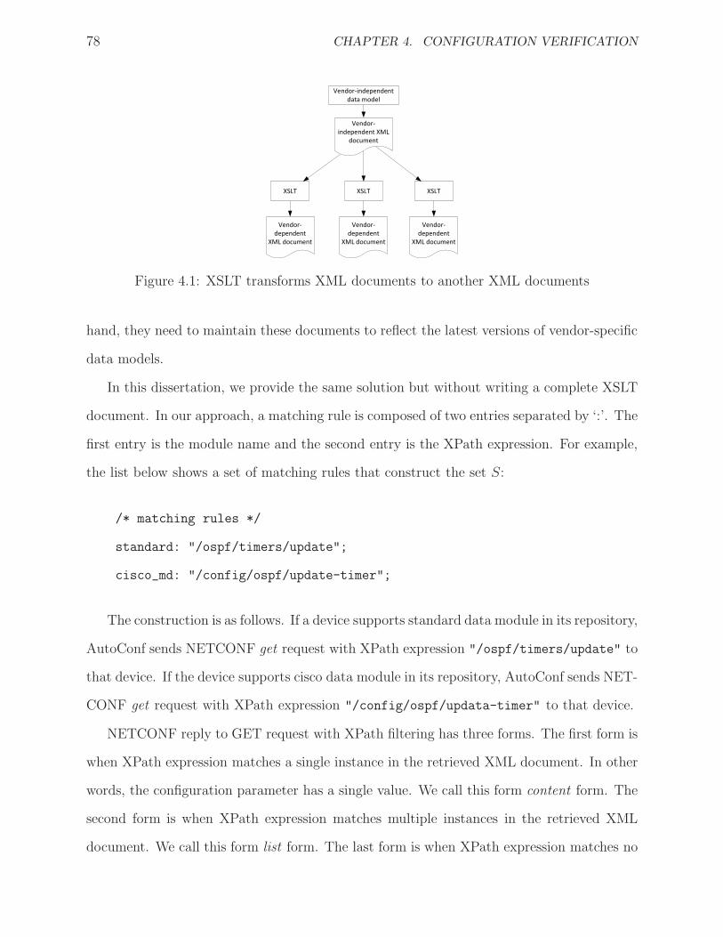
78 CHAPTER 4. CONFIGURATION VERIFICATION
Vendor-independent
data model
XSLT
Vendor-
independent XML
document
Vendor-
dependent
XML document
XSLT XSLT
Vendor-
dependent
XML document
Vendor-
dependent
XML document
Figure 4.1: XSLT transforms XML documents to another XML documents
hand, they need to maintain these documents to reflect the latest versions of vendor-specific
data models.
In this dissertation, we provide the same solution but without writing a complete XSLT
document. In our approach, a matching rule is composed of two entries separated by ‘:’. The
first entry is the module name and the second entry is the XPath expression. For example,
the list below shows a set of matching rules that construct the set S:
/* matching rules */
standard: "/ospf/timers/update";
cisco_md: "/config/ospf/update-timer";
The construction is as follows. If a device supports standard data module in its repository,
AutoConf sends NETCONF get request with XPath expression "/ospf/timers/update" to
that device. If the device supports cisco data module in its repository, AutoConf sends NET-
CONF get request with XPath expression "/config/ospf/updata-timer" to that device.
NETCONF reply to GET request with XPath filtering has three forms. The first form is
when XPath expression matches a single instance in the retrieved XML document. In other
words, the configuration parameter has a single value. We call this form content form. The
second form is when XPath expression matches multiple instances in the retrieved XML
document. We call this form list form. The last form is when XPath expression matches no
4.3. CONSISTENCY VERIFICATION 79
instance. The data node of the retrieved XML document is empty. For example, the XPath
expression "/interface["eth0"]/address" is expected to provide the IP address of eth0
interface (content form). However, the XPath expression "/interface/address" returns
the IP addresses of all interfaces (list form).
4.3.3 Link-level verification
In link-level verification, the set S consists of a set of pairs (xi, yi) where xi and yi represents
parameter values for two linked devices A and B, respectively. For example, the following
statement:
verify link [r1, r2]:interface {
content {
standard: "/interface/name[" ++ #interface.name ++"]/address";
cisco_md: "/interface/name/" ++ #interface.name ++"/ip-address";
}
assert all : subnet(X,24) == subnet(Y,24);
}
returns true if the IP addresses of the two interfaces sharing a common link have the same
subnet address. The function subnet() needs two arguments: an IP address and network
prefix. It returns the subnet address.
4.3.4 SCL Language Related to Consistency Verification
SCL supports consistency verification through verify construct. verify statement takes
two arguments as in manage statement: device and service identifiers. Consider the following
verification rule in SCL language:
verify *:ospf {
content {
80 CHAPTER 4. CONFIGURATION VERIFICATION
/* matching rules */
standard: "/ospf/timers/update";
cisco_md: "/config/ospf/update-timer";
}
assert all : int(X) >= 25 and int(X) <= 45;
}
The above verify rule says that for each device that supports ospf service, the update timer
should be between 25 and 45 seconds. AutoConf collects the information as follows. If the
device supports standard module in its repository, use the XPath “/ospf/timers/update” to
extract the correct parameter value. Otherwise, if it supports the vendor-specific cisco md
module, use the XPath “/config/ospf/update–timer”. Otherwise display a warning message.
content clause represents the set S while assert clause represents the consistency formula
as expressed in 4.1. The function int() is used to convert XML text to integer.
The following rule states that for each device, no non-equal interfaces are placed on the
same subnet with subnet prefix 24:
verify *:interfaces {
list {
standard : "/interface/address";
}
assert all : distinct(subnet(X, 24)); // 24 is subnet prefix
}
The SCL engine understands that the variable X is a list. So, the function subnet/2
returns another list that will be an argument for distinct/1 function. This function, in
turn, returns true if all elements in X are distinct.

4.3. CONSISTENCY VERIFICATION 81
4.3.4.1 High-order verification
Let
E1 ::= Q1 x ∈ S1 : F1(x)
E2 ::= Q2 x ∈ S2 : F2(x)
...
En ::= Qn x ∈ Sn : Fn(x)
be a set of verification rules. We wish to evaluate an expression that connects the above rules
using AND or OR logical operators. To do that, let S = {E1, E2, ..., En} and the constraint
expression is expressed in Equation 4.1. Since each element of S is eventually a Boolean
literal (true/false), the constraint expression can be reduced to Q e ∈ S : e is true. There
are three values of the quantifier Q that can be used here: all, some, and no. When the
value of the quantifier Q is all, then all e ∈ S : e is true is equivalent to E1 ∧E2 ∧ ...∧En,
when the value of quantifier Q is some, then some e ∈ S : e is true is equivalent to
E1 ∨ E2 ∨ ... ∨ En, and when the value of quantifier Q is no, then no e ∈ S : e is true is
equivalent to ¬E1 ∧ ¬E2 ∧ ... ∧ ¬En.
In SCL, high-order expressions are expressed by using eval clause. For example, the
statement
eval all {
verify r1:ospf { ... }
verify r2:ospf { ... }
verify link ...
}
returns true only if all verification rules return true.
You should notice that the statement above is by itself a verification rule. This means
we can embed this rule to a higher-order expression as shown below:

82 CHAPTER 4. CONFIGURATION VERIFICATION
eval some {
verify ... // E1
eval all {
verify ... // E2
verify ... // E3
}
} // E1 OR (E2 AND E3)
4.4 Behavioral Verification
One common function on all types of network devices is data forwarding, from an incoming
to an outgoing interface based on specific Forwarding Control List or FCL. For example,
FCL on a router is its routing entries in the routing table. FCL on a firewall is its access
control lists or ACLs. FCL on a NAT device is its address translation rules. Sometimes,
the functions of routing, access control, and address translation can be physically integrated
into one network device. In the following sections, we presents the formal representation of
firewall, routing and NAT policies, then we discuss the behavioral verification at link and
network levels.
4.4.1 Formal Representation of Forwarding Control List
An FCL, denoted as A, contains a set of rules, where each rule has a constraint over some
packet header fields and a decision. The decision of a rule depends on the type of FCL. A
typical decision of filtering FCL is accept or deny. A typical decision of routing FCL is the
outgoing interface or discard. For NAT FCL, a typical decision is to change some IP header
fields.
When analyzing an FCL, we need to determine the set of IP packets that will have the
same treatment. For example, when IP packets flow through a firewall device, the flow

4.4. BEHAVIORAL VERIFICATION 83
will be divided into a number of groups based on the number of decisions taken by the
firewall’s FCL. If the firewall has only two actions (say accept and deny), then the flow will
be divided into two groups: those packets that will be accepted and those packets that will
be denied. RFC 3917 defines a flow as a set of IP packets passing an observation point in
a network during a certain time interval. All packets belonging to a particular flow have a
set of common properties such that a property a is defined as a = f(x) where x can be:
1. one or more IP header field (e.g., source IP address), transport header field (e.g., source
port number), or application header field.
2. one or more characteristics of the packet itself (e.g., number of MPLS labels).
3. one or more of fields derived from packet treatment (e.g., next hop IP address).
We denote a flow as π. We say a packet p belongs to a flow π (e.g., p ∈ π) if it completely
matches all the defined properties of the flow. Without loss of generality we can assume,
in this chapter, that the flow properties are taken from the following packet header fields:
protocol, IP source address, IP destination address, source port address and destination
port address. To represent a set of IP packets, IP source address and IP destination address
are expressed in CIDR notation. Protocol and port addresses can be expressed as a single
value or a range of values. In CSM model, a flow is defined by the following tuple: {flow,
proto, srcip, dstip, srcport, dstport}. For example, the flow {flow, any, 10.1.2.0/24,
10.1.35.0/24, any, 1..1024} includes all possible packets originated from the subet 10.1.2.0/24
and destined to the subnet 10.1.35.0/24 with destination port ranges from 1 to 1024. The
set of all possible packets {flow, any, 0.0.0.0/0, 0.0.0.0/0, any, any} is denoted as Π.
FCL
policyΠ
π1
π2
πm
. . .
Figure 4.2: FCL policy with m different decisions partitioning flow Π into m sub–flows.

84 CHAPTER 4. CONFIGURATION VERIFICATION
In this dissertation, we focus on three types of FCLs that decide routing, access control
and address translation policies. The joint effect of the three FCLs will dominate flow
manipulation and network behavior. Our methodology is to formalize, in the first step, the
effect of the three FCLs on the flow Π as shown in Figure 4.2. As we mentioned before,
the effect of an FCL with m different decisions is to partition the flow Π into a set of m
sub–flows such that each sub–flow shares the same treatment. After that we develop a set
of algorithms to verify the configuration from link–level to network–level.
Verifying the current configuration of FCLs is important since FCLs are difficult to
configure correctly. There are several reasons. First, an FCL may consist of a large number
(e.g., thousands) of rules. Second, these rules may be written by different administrations
and at different times. Therefore, over the time, inconsistent FCL rules will be added that
may create security holes by allowing malicious traffic or blocking legitimate traffic.
Due to the complexity of FCLs, they are commonly transformed to formal mathemat-
ical logical models such as Binary Decision Diagram (BDD) or Firewall Decision Diagram
(FDD) [33], as we mentioned in Section 2.1. AutoConf adopts BDD due to its compactness,
canonicity, and ease of manipulation. The formal model of an FCL policy depends on its
type: filtering FCL, routing FCL or NAT FCL. However, we model an FCL rule, regardless
of its FCL type, as follows. The information we need about the packet is the flow properties
that we mentioned before. Therefore, we encode the information contained in a flow as a
sequence of Boolean variables such that
F = Fproto ∧ Fdstip ∧ Fsrcip ∧ Fdstport ∧ Fsrcport
where Fproto is a Boolean function of 8 variables, Fdstip and Fsrcip are Boolean functions of
32 variables, and Fdstport and Fsrcport are Boolean functions of 16 variables. To illustrate the
expression above, let us assume for simplicity that the IP address space is 2 bits and the
remaining fields are 1 bit. This implies that a flow can be encoded using 7 Boolean variables.
If a flow has the following information: srcip = 3, dstip = 2, proto = 0, srcport = any, and

4.4. BEHAVIORAL VERIFICATION 85
Set Operation BDD Operation DescriptionUnion OR (∨) F1 ∨ F2 represents the IP packets that satisfy F1 or F2
Intersection AND (∧) F1 ∧ F2 represents the IP packets that must satisfy F1
and F2
Not Negation (¬) ¬F = Π− FIs subset Imply (→) F1 → F2 means “is F1 ⊆ F2?” If the result ≡ true
(tautology) then F1 is a subset of F2
Table 4.2: Set operations and their equivalent BDD operations
dstport = 1. Then,
Fproto(x0) = ¬x0,
Fdstip(x1, x2) = x1 ∧ ¬x2,
Fsrcip(x3, x4) = x3 ∧ x4,
Fdstport(x5) = x5, and
Fsrcport(x6) = 1.
where xi is a Boolean variable that can take either 0 or 1. Notice that there are two
assignments to bits/variables that satisfies F (i.e., F is true): first assignment is F =
Fproto(0) ∧ Fdstip(1, 0) ∧ Fsrcip(1, 1) ∧ Fdstport(1) ∧ Fsrcport(0) and the second assignment is
F = Fproto(0)∧Fdstip(1, 0)∧Fsrcip(1, 1)∧Fdstport(1)∧Fsrcport(1). Hence, F represents a “set”
of two IP packets.
In summary, the semantic of a Boolean function (or expression) in our analysis is that it
models a complex set. BDD provides compact representations for Boolean expressions, and
it supports semantically set operations as shown in Table 4.2.
Now, let r = 〈cproto, cdstip, csrcip, cdstport, csrcport, a〉 be an FCL rule where cx is a constraint
over the field x and a is an action to be taken. The Boolean expression of the rule r, denoted
as Fr, is
Fr = Fa ∧ Fc (4.2)
where
Fc = Fproto ∧ Fdstip ∧ Fsrcip ∧ Fdstport ∧ Fsrcport (4.3)
86 CHAPTER 4. CONFIGURATION VERIFICATION
and Fa is a Boolean function of 8 variables. This implies the total number of Boolean vari-
ables to model an FCL rule is 112 variables. The interpretation of the field action depends
on the FCL type. For example, in routing policy, the field action encodes (forwarding to)
the outgoing interface. Notice that the Boolean expression Fc encodes a set of IP packets
that satisfy Fc and hence Fc represents a flow.
We introduce three functions to manipulate Boolean expressions, which are the projection
function, its inverse function, and the mask function.
Projection function : is defined as Ψ : Fπ × P → Fa, where Fπ, P , and Fa are Boolean
expressions for a flow, an FCL policy and an action, respectively. Ψ is used to determine the
set of actions applied to an incoming flow π. For example, if P represents a routing FCL,
then Ψ(π, P ) will return a Boolean expression that represents the set of outgoing interfaces
that will be used to forward each packet in flow π.
Inverse of projection function : is defined as Ψ−1 : Fa×P → Fπ, is used to determine the
set of IP packets that will be treated according to the actions encoded in Fa. For example,
if P is a filtering FCL and we need to determine the set of IP packets that will be denied,
then we will use Ψ−1(Fdeny, P ) given that Fdeny is the Boolean expression to encode ”deny”
action.
Mask function : is defined as τ : F × h → F ′ that takes as arguments two Boolean
expressions F and h, and returns a new Boolean expression F ′ by resetting F at locations
defined in h using existential quantifier operator. For example, if a flow is any packet sourced
from 10.1.2.0/24 and destined to 10.1.23.0/24, applying τ function will result in a flow of
any packet sourced from 10.1.2.0/24 given that h = Fdstip.
In all our discussion, we denote the Boolean expression of an FCL policy as P .
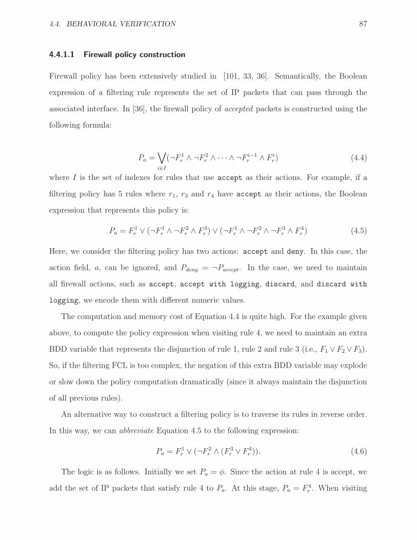
4.4. BEHAVIORAL VERIFICATION 87
4.4.1.1 Firewall policy construction
Firewall policy has been extensively studied in [101, 33, 36]. Semantically, the Boolean
expression of a filtering rule represents the set of IP packets that can pass through the
associated interface. In [36], the firewall policy of accepted packets is constructed using the
following formula:
Pa =∨
i∈I
(¬F 1r ∧ ¬F
2r ∧ · · · ∧ ¬F
i−1r ∧ F i
r) (4.4)
where I is the set of indexes for rules that use accept as their actions. For example, if a
filtering policy has 5 rules where r1, r3 and r4 have accept as their actions, the Boolean
expression that represents this policy is:
Pa = F 1r ∨ (¬F 1
r ∧ ¬F2r ∧ F 3
r ) ∨ (¬F 1r ∧ ¬F
2r ∧ ¬F
3r ∧ F 4
r ) (4.5)
Here, we consider the filtering policy has two actions: accept and deny. In this case, the
action field, a, can be ignored, and Pdeny = ¬Paccept. In the case, we need to maintain
all firewall actions, such as accept, accept with logging, discard, and discard with
logging, we encode them with different numeric values.
The computation and memory cost of Equation 4.4 is quite high. For the example given
above, to compute the policy expression when visiting rule 4, we need to maintain an extra
BDD variable that represents the disjunction of rule 1, rule 2 and rule 3 (i.e., F1 ∨F2 ∨F3).
So, if the filtering FCL is too complex, the negation of this extra BDD variable may explode
or slow down the policy computation dramatically (since it always maintain the disjunction
of all previous rules).
An alternative way to construct a filtering policy is to traverse its rules in reverse order.
In this way, we can abbreviate Equation 4.5 to the following expression:
Pa = F 1r ∨ (¬F 2
r ∧ (F 3r ∨ F 4
r )). (4.6)
The logic is as follows. Initially we set Pa = φ. Since the action at rule 4 is accept, we
add the set of IP packets that satisfy rule 4 to Pa. At this stage, Pa = F 4r . When visiting

88 CHAPTER 4. CONFIGURATION VERIFICATION
rule 3, we also add the set of IP packets that satisfy rule 3 to Pa. At this stage, Pa = F 3r ∨F
4r .
When visiting rule 2, we need to remove those packets p such that p ∈ Pa and p ∈ F 2r since
rule 2 has higher priority than rule 3 and 4. At this stage, Pa = ¬F2r ∧(F
3r ∨F
4r ). Finally, we
visiting rule 1, we add the packets that satisfy rule 1 to Pa. As a result, we get Equation 4.6.
The above operations can be expressed as a recursive Boolean function T , such that:
T (i) =
ai == accept→ T (i+ 1) ∨ F ir , T (i+ 1) ∧ ¬F i
r
if 1 ≤ i < N
ai == accept→ F ir , false i = N
(4.7)
where a→ b, c represents if–then–else operator (If a is true, then b, otherwise c). Therefore,
the filtering policy P is computed as
P = T (1)
The construction algorithm needs only a single Boolean expression, say T , that will be
updated while traversing the FCL rules in reverse order. We compared the performance
of two algorithms that implement Equation 4.4 and Equation 4.7 with the same variable
ordering. The experimental results discussed in Section 4.4 demonstrate that our formal-
ization can achieve significant improvement on memory and computation efficiency over the
previous work. In the case where Equation 4.4 has exploded, our formalization constructed
the same firewall policy in just a few seconds.
The filtering policy P = Pa determines the set of IP packets that are allowed to bypass.
Therefore, if a flow π passes through a filtering FCL, the set of packets that are permitted
can be expressed as:
Fπ ∧ P (4.8)
When configuring a filtering policy, the policy is usually applied to a network interface.
A filtering FCL that is applied to an incoming traffic is called an inbound FCL. A filtering
FCL that is applied to an outgoing traffic is called an outbound FCL. If a network device is
configured with an inbound FCL and an outbound FCL, a traffic flow may pass both FCLs.

4.4. BEHAVIORAL VERIFICATION 89
To compute the effect of inbound and outbound FCLs on network traffic, we model
a physical interface as two unidirectional logical interfaces. Each physical interface has a
unique number (within a device) as specified in CSM model. Therefore, a unidirectional
logical interface is identified by its physical interface number along with a flag bit. The flag
bit determines whether the logical interface is designated for incoming (0) or outgoing (1)
traffic.
We aim at constructing a single Boolean expression that represents all filtering FCLs in
a device so that complex verification queries can be efficiently handled. Let i be an interface
number, d be a direction (0 for “in” and 1 for “out”), P 0i be the Boolean expression of the
inbound FCL at network interface i, and P 1i be the Boolean expression of the outbound
FCL at network interface i. P di is computed using Equation 4.7. The overall filtering policy
for a network device is expressed as:
P =∨
i∈{1...I},d∈{0,1}
(Fi ∧Hd ∧ P di ) (4.9)
where I is the total number of network interfaces, Fi is the Boolean expression of the
numeric value i and Hd is the Boolean expression of the flag bit d. Please note that if a
unidirectional interface does not employ a filtering policy, its Boolean expression will become
true to indicate the acceptance of all possible packets.
The Boolean variables to encode i and d are located within the action field. Since
action field uses 8 bits, the the maximum value of I is 128. Therefore, we can express Fa
as Fa = Fi ∧Hd. As a result, if a flow π passes through interface i at direction d, the set of
packets that are allowed is given by:
Fπ ∧ P di = Fπ ∧Ψ−1(Fi ∧Hd, P ) (4.10)
where P is given in Equation 4.9.
Another common verification query is to find the set of packets that may pass a device
from any incoming interfaces to a specific outgoing interface. This query is particularly
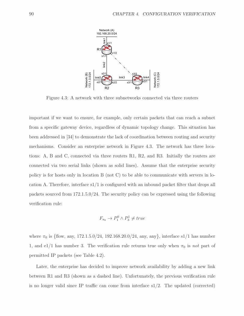
90 CHAPTER 4. CONFIGURATION VERIFICATION
R1
R2 R3
link2
link3
Network (A)
192.168.20.0/24
Network (C)
172.1.5.0/24
Network (B)
172.1.3.0/24
s1/1
s1/2
s2/2
s2/1
e1/1
e2/1
s3/2
s3/1 e3/1
link1
link4link5
Figure 4.3: A network with three subnetworks connected via three routers
important if we want to ensure, for example, only certain packets that can reach a subnet
from a specific gateway device, regardless of dynamic topology change. This situation has
been addressed in [34] to demonstrate the lack of coordination between routing and security
mechanisms. Consider an enterprise network in Figure 4.3. The network has three loca-
tions: A, B and C, connected via three routers R1, R2, and R3. Initially the routers are
connected via two serial links (shown as solid lines). Assume that the enterprise security
policy is for hosts only in location B (not C) to be able to communicate with servers in lo-
cation A. Therefore, interface s1/1 is configured with an inbound packet filter that drops all
packets sourced from 172.1.5.0/24. The security policy can be expressed using the following
verification rule:
Fπ0→ P 0
1 ∧ P 13 6= true
where π0 is {flow, any, 172.1.5.0/24, 192.168.20.0/24, any, any}, interface s1/1 has number
1, and e1/1 has number 3. The verification rule returns true only when π0 is not part of
permitted IP packets (see Table 4.2).
Later, the enterprise has decided to improve network availability by adding a new link
between R1 and R3 (shown as a dashed line). Unfortunately, the previous verification rule
is no longer valid since IP traffic can come from interface s1/2. The updated (corrected)

4.4. BEHAVIORAL VERIFICATION 91
verification rule is
Fπ0→
[
(P 01 ∧ P 1
3 ) ∨ (P 02 ∧ P 1
3 )]
6= true
where inteface s1/2 has number 2.
In order to define a verification rule that is valid regardless of any topology change, we
can express E = (P 01 ∧ P 1
3 ) ∨ (P 02 ∧ P 1
3 ) as
E = (P 01 ∧ P 1
3 ) ∨ (P 02 ∧ P 1
3 )
= P 13
∧
(P 01 ∨ P 0
2 )
= Ψ−1(F3 ∧H1, P )∧
Ψ−1(¬F3 ∧H0, P )
Therefore, given the outgoing interface n and policy P , the verification rule is
Fπ0→ Ψ−1(Fn ∧H1, P )
∧
Ψ−1(¬Fn ∧H0, P ) 6= true (4.11)
4.4.1.2 Routing policy construction
Unlike firewalls, routers do not select next hop based on the order of routing rules, but would
rather find the longest prefix match. In addition, most routers support load-balancing when
multiple paths exist. This implies multiple routing rules can be applicable to the same flow
with their corresponding actions.
Each routing rule in routing policy is composed of a single matching field, which is
the destination IP address. The action is forwarding packets to the next hop, which is
determined by the outgoing interface along with the IP address of the next hop.
We construct the Boolean expression of a routing policy as follows. For each network
prefix of length m, we first construct Pm and P cm such that
Pm =∨
k∈Im
F kr and P c
m =∨
k∈Im
F kc
where Im represents the set of indexes for the entries that have destination prefix of length
m, F kc represents the Boolean expression of the rule constraint without the action field
(See Equation 4.3), and F kr is the Boolean expression of a routing entry as expressed in
92 CHAPTER 4. CONFIGURATION VERIFICATION
Equation 4.2. The Boolean expression of the action field is expressed as Fa = Fi∧H1, where
i is the interface number. Then, we construct the routing policy, P , using the following
recursive equation:
T (m) =
Pm ∨ (¬P cm ∧ T (m− 1)) 1 ≤ m ≤ 32,
P0 m = 0(4.12)
where P = T32.
Applying the projection function Ψ on a routing policy P and a flow π (i.e., Ψ(Fπ, P ))
produces three possible outcomes:
1. The flow π is completely forwarded either to a single interface or multiple interfaces
(i.e., ∀p ∈ π, the packet p will be forwarded to the next hop),
2. The flow π is completely discarded (i.e., Ψ(Fπ, P ) == false), and
3. The flow π is partially forwarded (i.e., ∃p, q ∈ π and p 6= q , the packet p will be
forwarded while the packet q will be discarded).
To ensure that the flow π has been completely forwarded by the routing FCL, we use the
following verification rule
Fπ → Ψ−1(Ψ(Fπ, P ), P ) = true (4.13)
Usually, we like to focus whether or not a flow π can reach a specific device. In other
words, if the flow π passes through a router device, what flow that will be forwarded to the
outgoing interface i? We answer this query using the following expression:
Fπ ∧Ψ−1(Fi ∧H1, P ) (4.14)
4.4.1.3 NAT policy construction
Network Address Translation, NAT, is used by a device (e.g., firewall, router) deployed
between a private and public networks. There are three forms of NAT FCLs: static NAT

4.4. BEHAVIORAL VERIFICATION 93
FCL, dynamic NAT FCL, and overloading NAT (also known as PAT) FCL. In static NAT
FCL, each rule translates a given source IP address to another pre-allocated source IP
address. In dynamic NAT FCL, each rule translates a group of source IP addresses to
another pre-allocated group of IP addresses. In overloading NAT FCL, each rule translates
a group of source IP addresses to a single pre-allocated IP address but with different source
ports.
Basically, a NAT rule is composed of a constraint over the source header field along with
an action that determines the new source address. If an IP packet that is traversing from
a private to public network matches the constraint, the source IP address of the packet will
be replaced with the IP address specified in the action field. Otherwise, the packet will
be passed without translation. The device that supports NAT service also keeps a reverse
translation for the packets that are traversing from public to private network.
Modeling NAT FCL requires extra bits (up to 48 bits) to encode the action. This
implies changing the number of bits dedicated for action field from 8 to 48 bits. To unify the
encoding, we break a NAT rule (c→ a) into two rules: c→ i and a→ i where i is the rule
index. This solution is valid because the number of rules in NAT FCL is usually very small.
Using this scheme, the maximum possible number of rules for a NAT FCL is 256 rules.
Let Ac be the list that represents c→ i and Aa be the list that represents a→ i. Let Pc
and Pa be the Boolean expressions for Ac and Aa, respectively. We calculate Pc and Pa as
follows:
Pc =N∨
i
Fi ∧ Fc
and
Pa =N∨
i
Fi ∧ Fa,
where N is the number of rules in A.
While constructing the Boolean expressions of Pc and Pa, we also construct Pc and Pa
to represent the reverse translation when a flow is traversing from public back to private
network. A constraint over the source IP address encoded in Pc becomes the constraint over

94 CHAPTER 4. CONFIGURATION VERIFICATION
the destination IP address encoded in Pc. We do the same encoding for Pa. Therefore, for
each NAT or PAT service, we maintain four policies: Pc, Pa, Pc and Pa.
Now, let π be a flow that traverses from private to public network and passes through a
static or dynamic NAT service, the effect of NAT service on the flow is expressed as
T (Pc ∧ Fπ) ∨ (¬Pc ∧ Fπ), (4.15)
where ¬Pc ∧Fπ is the set of packets that pass NAT service without translation, and Pc ∧Fπ
is the set of packets that have been translated under the transformation function T , and
T (x) = τ(x, Fsrcip) ∧Ψ−1(Ψ(x, Pc), Pa).
In case of PAT, we replace Fsrcip with the expression Fsrcip ∧ Fsrcport.
The effect of NAT service on the flow π when traversing from public network to private
network is expressed as
T−1(Pa ∧ Fπ) ∨ (¬Pa ∧ Fπ), (4.16)
where
T−1(x) = τ(x, Fdstip) ∧Ψ−1(Ψ(x, Pa), Pc).
In case of PAT, we replace Fdstip with the expression Fdstip ∧ Fdstport.
4.4.2 Link-level Behavior
Network behavior in terms of reachability and security is based on the behavior of each link
in the network. We define a link behavior as the set of all possible packets passing through
the link at any given time. Consider the enterprise network example in Figure 4.3. A host at
location A sends an IP packet to a host at location C. The IP packet can reach subnetwork
C if the network is configured properly to allow this packet passes through link 1, link 2,
link 3 and link 4 as shown in Figure 4.3. The direction of the flow in link 1 is from network
A to interface s2/1, the direction in link 2 is from interface s1/1 to interface s2/1, and so
on. Therefore, the flow that passes through link 4 from R4 to network C at any given time

4.4. BEHAVIORAL VERIFICATION 95
determines the set of IP packets reachable to hosts in network C. This flow relies mainly
on another flow that passes link 3 from R2 to R3. Consequently, if we determine what IP
packets permitted to flow from R2 to R3, then we can determine the IP packets permitted
to flow from R3 to network C.
In CSM model, network links are modeled by using link primitive. Each link has a class
and ports. The attribute class determines the link type (such as Ethernet, Serial or any
user–defined class) while ports define the end points. In addition, each link is associated
with one or two unidirectional connection primitives. Connection primitives are created by
predefined rules based on the link class. For example, in case of “ethernet” and “serial”
classes, we define two unidirectional connections. A connection tuple is defined as {connect,
id, dev1, port1, dev2, port2, F} where id is a universal identification number, F , which
will be explained later, is a Boolean expression, and the connection direction is from dev1
to dev2. For example, {link, ethernet, undefined, [{r1, 1}, {r2, 1}]} creates two predicates:
{connect, 1, r1, 1, r2, 1, true} and {connect, 2, r2, 1, r1, 1, true}.
The Boolean expression F expresses the “local” effect of its connection on a flow. This
effect results from applying FCL policies on this connection. Let us consider the connection
from R1 to R2 as shown in Figure 4.3. The FCL policies that affect any flow passes through
this connection are: routing FCL on R1, NAT FCL on R1, filtering (outbound) FCL applied
on interface s1/1, and filtering (inbound) FCL applied on interface s2/1. Thus, for this
connection and ignoring NAT policy, F is expressed as:
FΠ ∧Ψ(F1 ∧H1, PR1routing) ∧Ψ(F1 ∧H1, P
R1filtering) ∧Ψ(F1 ∧H0, P
R2filtering)
If NAT policy should be applied, then F is given as:
V = FΠ ∧Ψ(F1 ∧H1, PR1routing)
[
T (V ∧ PR1NAT ) ∨ (¬V ∧ PR1
NAT )]
∧Ψ(F1 ∧H1, PR1filtering) ∧Ψ(F1 ∧H0, P
R2filtering)
Algorithm 1 shows the steps to compute the Boolean expression F for each connection.
We follow the order of operations based on many network devices such as Cisco devices.

96 CHAPTER 4. CONFIGURATION VERIFICATION
Algorithm 1 Updating Connection ExpressionInput: The connection conn
Output: The connection conn
1: {connect, ID, D1, P1, D2, P2, } = conn/* Process outgoing interface */
2: Fπ ← true /* i.e. any possible flow */3: if D1 has Routing then
4: Fπ ← Apply Eqn 4.145: end if
6: if D1 has NAT and P1 is external then7: Fπ ← Apply Eqn 4.158: end if
9: if D1 has Filtering at P1 then
10: Fπ ← Apply Eqn 4.1011: end if
/* Process Incoming interface */12: if D2 has Filtering at P2 then
13: Fπ ← Apply Eqn 4.1014: end if
15: if D2 has NAT and P2 is internal then16: Fπ ← Apply Eqn 4.1617: end if
18: return {connect, ID, D1, P1, D2, P2, Fπ}
4.4.3 Network-level Behavior
The Boolean expression F captures the local effect of a connection on a flow. This expression
tells us the set of all possible IP packets permitted to pass through at any given time.
However, it does not tell us the “effective” IP packets that will flow through the connection.
Some IP packets may be blocked or discarded before they reach the connection. In Figure 4.3,
the effective IP packets that pass through the connection from R3 to network C are coming
from link 3. The effective IP packets that pass through link 3 (from R2 to R3) are resulted
from link 2 plus link 5. Thus, if we determine the effective IP packets that pass through a
connection, we can evaluate the network behavior.
We model a network topology as a directed graph G = 〈V,E〉, where V is the set of
vertices and E is the set of edges. Each vertex v ∈ V represents a unidirectional connection
and it is labelled by its connection id. A directed edge [u, v] in G is constructed when the
following two conditions hold:
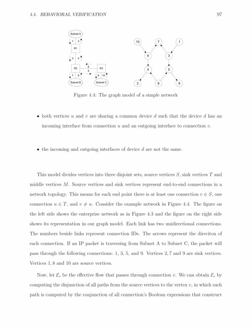
4.4. BEHAVIORAL VERIFICATION 97
R1
R2
Subnet A
R3
Subnet B Subnet C
3 4
7
36
10 1
54
82 9
21
10
6
5
7 8 9
Figure 4.4: The graph model of a simple network
• both vertices u and v are sharing a common device d such that the device d has an
incoming interface from connection u and an outgoing interface to connection v.
• the incoming and outgoing interfaces of device d are not the same.
This model divides vertices into three disjoint sets, source vertices S, sink vertices T and
middle vertices M . Source vertices and sink vertices represent end-to-end connections in a
network topology. This means for each end point there is at least one connection v ∈ S, one
connection u ∈ T , and v 6= u. Consider the example network in Figure 4.4. The figure on
the left side shows the enterprise network as in Figure 4.3 and the figure on the right side
shows its representation in our graph model. Each link has two unidirectional connections.
The numbers beside links represent connection IDs. The arrows represent the direciton of
each connection. If an IP packet is traversing from Subnet A to Subnet C, the packet will
pass through the following connections: 1, 3, 5, and 9. Vertices 2, 7 and 9 are sink vertices.
Vertices 1, 8 and 10 are source vertices.
Now, let Ev be the effective flow that passes through connection v. We can obtain Ev by
computing the disjunction of all paths from the source vertices to the vertex v, in which each
path is computed by the conjunction of all connection’s Boolean expressions that construct

98 CHAPTER 4. CONFIGURATION VERIFICATION
the path. For example,
E5 = (F5 ∧ F8) ∨ (F5 ∧ F3 ∧ F1)
= F5 ∧ [F8 ∨ (F3 ∧ F1)]
= F5 ∧ (E8 ∨ E3)
where E8 = F8 and E3 = F3 ∧ E1.
Algorithm 2 describes a depth first search algorithm to compute Et where t ∈ T . The
network–level behavior can then be computed by applying Algorithm 2 for each sink vertex.
This algorithm ensures that Ev is computed only once unless v is included in a loop. In this
case, for each sink vertex we reset those vertices that are included in some loop by marking
them as unvisited and setting its E ’s value to false. The reason of resetting is to ensure
correct computation when AutoConf receives initial configuration with no information about
routing policies. Ignoring the cost of BDD operations, the running time over all sink vertices
using Algorithm 2 is O(|L| × |T |) where L represents the set of vertices that are included in
some cycle in the graph G.
4.4.4 Impact of Configuration Change
Here we show how AutoConf handles configuration change efficiently. We distinguish be-
tween two impacts of dynamic configuration: Network topology change and Connection
change. Network topology change occurs when adding or removing physical links or any
modification that triggers routers to update their routing tables. When it occurs, we need
to rebuild routing policies, and recompute F and E values. Connection change is any mod-
ification that occurs at specific connection like modifying ACL rules for a specific service or
updating Subnet addresses. For example, in Figure 4.4, if we add a new inbound filtering
policy in connection 4 at router R1, then we need to rebuild the BDD of filtering policy of
router R1 using Equation 4.10, next we recompute F4 using Algorithm 1, and finally we
need to update E4 by using Algorithm 3. The running time of Algorithm 3 is O(|V |).

4.4. BEHAVIORAL VERIFICATION 99
Algorithm 2 Algorithm to construct E of vertex t ∈ T
Input: The graph G = 〈V,E〉 and vertex t ∈ T
Output: The set of E1: set t′ ← the opposite connection of t2: store the status of t′ and Et′
3: mark t′ as visited and set Et′ ← false
4: reset all vertices in V that are involved in a cycle5: compute(t)
6: restore t′ to its original values
Procedure: compute(v)
1: if v is not visited then
2: mark v as visited3: if v ∈ S then
4: Ev ← Fv
5: else
6: X ← false
7: for all u ∈ V such that [u, v] ∈ E do
8: compute(u)
9: X ← X ∨ Eu10: end for
11: Ev ← Fv ∧X
12: end if
13: end if
Algorithm 3 Algorithm to update E of vertex v ∈ VInput: The graph G = 〈V,E〉 and vertex v ∈ V
Output: The updated set of E1: reset all vertices in V that are involved in a cycle2: update(v, v)
Procedure: update(v, t)
1: mark v as unvisited2: compute(v)3: for all u ∈ V such that [v, u] ∈ E do
4: if u == t then
5: continue
6: else
7: update(u, t)
8: end if
9: end for
4.4.5 SCL Language Related to Behavioral Verification
SCL supports two types of queries: show query and assert query. Show query displays either
the set of packets that represents a flow or the set of actions performed on a given flow.

100 CHAPTER 4. CONFIGURATION VERIFICATION
Assert query provides true/false answers.
4.4.5.1 SHOW Query
The general syntax of show query is:
policy <device>|list|* : <action>|* {
[show <flow>|<action>
when (<constraint>) [;]]+
}
The constraint field consists a set of field = value conditions where field can be proto,
srcip, dstip, srcpx (src subnet mask), dstpx (dst subnet mask), srcport, dstport,
action, oface (for outgoing interface), iface (for incoming interface). The value can be
an atom, integer, IPv4 address, IPv4 address/prefix, or a list (enclosed by []). For example,
we need to display what actions (outgoing interface) will be taken when a given flow passes
through a routing policy in router r2. The query is:
policy r2 : routing { // service-level
show action when (dstip = 10.2.3.0/24);}
The next query displays the set of packets that passes router r1 through outgoing interface 2:
policy r1 : * { // device-level
show flow when (oface = 2) }
4.4.5.2 ASSERT Query
The SCL format for assert statement is
policy <device>|list|* : <action>|* {
[ assert ( <constraint> ) ]+
}

4.5. SUMMARY 101
The following query returns 1 (true) if there is a path from subnet s1 to a Web server in
subnet s2:
policy [s1, s2]:path {
assert (action=1, dstip=72.10.2.101, dstport=80) }
Two or more assert statements can be connected logically by using eval statement. The
eval statement is based on the following formula: Q : F where Q is quantifier that can take
the following values: all, some, or none and F is a set of logical functions. For example,
the following query ensures that there is a connection between subet s1 and the Web server
at subnet s2:
eval all {
policy [s1, s2]:path {
assert (action=1, dstip=72.10.2.101, dstport=80);}
policy [s2, s1]:path {
assert (action=1, srcip=72.10.2.101, srcport=80);}
}
4.5 Summary
With the increasing complexity of network configuration, verifying network behavior is an
essential activity to ensure the correct operation of a network. This chapter presents a
configuration verification solution that partition the problem space into two categories: con-
sistency verification and behavioral verification. We present a formalization methodology to
verify the consistency of configuration parameters that span multiple network devices. In
behavioral verification, we present a graph-based model along with Binary decision diagram
(BDD) to formally capture the network behavior in terms of reachability and security. In
addition, we extend Structure Configuration Language (SCL) to provide an expressive query
interface for network administrators.

Chapter 5
Configuration Automation
5.1 Overview
Managing IP networks is considered a challenging task due to several factors: heterogeneous
network, deployment of various network services and guaranteeing its quality of service,
different provisioning requirements, and primitive support from network devices. To mitigate
management complexity, there is a growing consensus about the need for an automated
network management system especially for environment where it requires quick services
deployment, almost near to real-time to avoid service disruption such as tactical military
environment [18, 92].
Policy–driven management is the most widely adopted approach for network manage-
ment. As reported by Chen at. el. [19], Tier-1 Internet service provider (ISP) and enterprise
networks are managed by following a standard practice called method of procedure (MOP).
This practice is basically a policy–based approach under which there are a set of rules gov-
erning the choices of desired network behavior. Each rule consists of a set of actions to be
performed and a set of conditions to be checked before such actions can be taken.
The main features of policy–based management are its flexibility and scalability for
managing complex, large–scale networks [23]. Scalability is achieved by applying the same
103

104 CHAPTER 5. CONFIGURATION AUTOMATION
policy rule to large sets of devices and services, while flexibility is achieved by separating
the policy from the implementation of the managed system. Policy–based management is
widely adopted by IETF and DMTF standard organizations.
This chapter focuses on managing and automating IP network configuration using policy–
based management. In this context, required or desired behavior of network operations and
its services are expressed in terms of policies. These policies are enforced by AutoConf
by sending NETCONF configuration commands as illustrated in Figure 5.1. Automating
network configuration using policy–based approach has several challenges. The following
paragraphs describe them.
As we mentioned, policy rules are specified in a high-level language in order to reduce the
configuration complexity. For example, a policy may state that if there is a network interface
in Subnet 1 that does not belong to the network address 10.1.1.0/24, then invoke the action
ifconfig() with appropriate parameter values. This rule is applied to multiple devices where
each device supports multiple interfaces. In order to enforce this rule, the system must check
the IP address of each network interface in Subnet 1. If it finds one interface that does not
comply to the policy, it will trigger ifconfig() action on that interface. Now, if the manager
has defined many policies and the network has experienced multiple changes (the system
will be notified by a monitoring system), the management system should iterate over the
policy rules for each change to determine the set of actions along with the parameter lists.
The problem will be exacerbated if these policies are complex, having multiple conditions
connected by Boolean operators (such as AND, OR, etc.). Moreover, the management
cannot only rely on the current changes to determine the set of actions but also on the
previous changes. Because when the management system aggregates the previous and the
new changes, the satisfiability of some policies might be completed. In other words, all
conditions for those policies are met. Therefore, our first challenge is to develop a model
that captures the complexity of the policy rules as well as the current network state efficiently.
The model should allows us to easily discover any inconsistency or conflict within a policy.

5.1. OVERVIEW 105
Manager System
(AutoConf)
Monitor system
Policy Rules
Database
Managed network
Policy
Enforcement
(via NETCONF)
Learning
Agent
Figure 5.1: Policy–based management
The second challenge is that the model should scale well in large–scale networks. If a
network consists of hundreds of devices, the network state will be huge specially when the
network is running several services.
The last challenge is that the management system may face multiple actions that should
decide on an action or strategy to handle any conflict during network operation. In order
to decide the most effective strategy, the management system should have a detailed infor-
mation of each element in the network. This will improve the correlation accuracy when
the system is trying to correlate the current network state and the current policies with the
expected future network state. This correlation enables the management system to learn
from its past experience and optimize the selection of future actions.
Considerable research work has been done on policy–based management (see Section 2.5).
Most work mainly focused on building policy–based framework, policy specification and pol-
icy language. In environment where multiple policy rules may be triggered, policy selection
is often based on statically configured work–flow [19] performed by an administrator. As
the network becomes more complex; however, policies will be deficient to handle and tackle
unseen work–flow. In this case, human involvement is required and manual configuration
is performed which may generate misconfiguration. Therefore, it is imperative for config-
uration management system to automate policy selection in order to deal with not only
configuration process but also misconfiguration that may occur. Several researches [7, 91]
106 CHAPTER 5. CONFIGURATION AUTOMATION
have proposed approaches to implementing policy adaptation. These approaches consider
system automation in a single device. Due to the complexity of policy rules and the dif-
ficulty to represent network state, there are a few attempts in policy adaptation [6, 95].
This chapter presents an attempt to implement Reinforcement Learning (RL) for large-scale
network.
We use Binary Decision Diagram (BDD) to tackle the complexity of network descrip-
tion and resolve the aforementioned challenges. BDD has been used to formally represent
service–oriented policies such as Firewall and IPSec where the number of parameters (such
as IP header parameters) is limited and very few. We show how we can represent a formal
model for a large set of parameters that belong to different services spanning over multiple
network devices. We propose a set of formal models to capture the policy rules and net-
work operational status. We use RL technique called Q-learning that allows AutoConf to
learn in real–time in order to figure out the best strategy to handle any conflict or any QoS
degradation according to an existing set of requirements.
5.2 Policy Structure
There are several policy languages that specify policy rules and actions. We focus here on
the logical representation. We assume a policy is consisting of a set of rules such that each
policy rule has a conjunctive set of conditions along with a list of actions that change the
network behavior. A policy rule may have other attributes such as policy name, policy type
and whether the rules is enabled or not [24]. Formally, we define a policy rule as a tuple
p = 〈C,A〉 where C is a list of conditions, and A is a list of actions.
5.2.1 Policy Condition
Policy conditions are based on metrics that describe the network behavior such as flow char-
acteristics (e.g., Type of Service or ToS IP header field), traffic parameters (e.g., round–trip

5.2. POLICY STRUCTURE 107
delay, jitter or throughput), performance parameters (e.g., link utilization, link bandwidth,
packet loss probability), and configuration parameters (e.g., network interfaces’ status, en-
abled network protocols such as OSPF or ISIS). Moreover, many enterprises and ISP net-
works rely on service level agreement (SLA) to guarantee QoS to end users or applications.
These SLAs are eventually a set of QoS metrics. For example, an enterprise network es-
tablishes an SLA that states “A video application between clients in site A and a media
streaming server in site B should receive Gold service” [60]. The network administrator
defines “Gold service” as a network service with lowest delay and lowest packet loss, and
Differentiated Service architecture is deployed in the network.
We define a policy condition c ∈ C as c = 〈 metric-spec,V 〉, where V is an interval of
values. We define metric–spec as a tuple m = 〈 target-name, service-name, metric-name
〉. For examples:
1. the status of interface e1/1 in router R1 can be expressed as 〈R1, interface, e1/1〉,
2. all interfaces in router R1 can be expressed as 〈R1, interface, any〉,
3. the number of clients accessing the media streaming server server01 can be expressed
as 〈server01, mediaStreaming, num-clients〉, and
4. link x bandwidth can be expressed as 〈x, link, bandwidth〉.
A policy condition c is a relational expression that has a relational operator such as
“=”, “ 6=”, “<”, “≤”, “>”, or “≥”. As such, the relational expression identifies the set
of values (i.e., V) under which an action a ∈ A will be executed. The set V can be a
single value (e.g., if <R1,interface,e1/1> == false then action--list()), or it can
be a range of values (e.g., if <Server01, mediaStreaming, num-clients> > 100 then
action--list()). In our analysis, the set V is always expressed as an interval. Table 5.1
summarizes the relationships between the set V and the relational operators.
We assume that all metrics used to describe the network behavior are 64-bit non-negative
integer values. In case of Boolean metrics, we use the values 1 and 0 to indicate true and
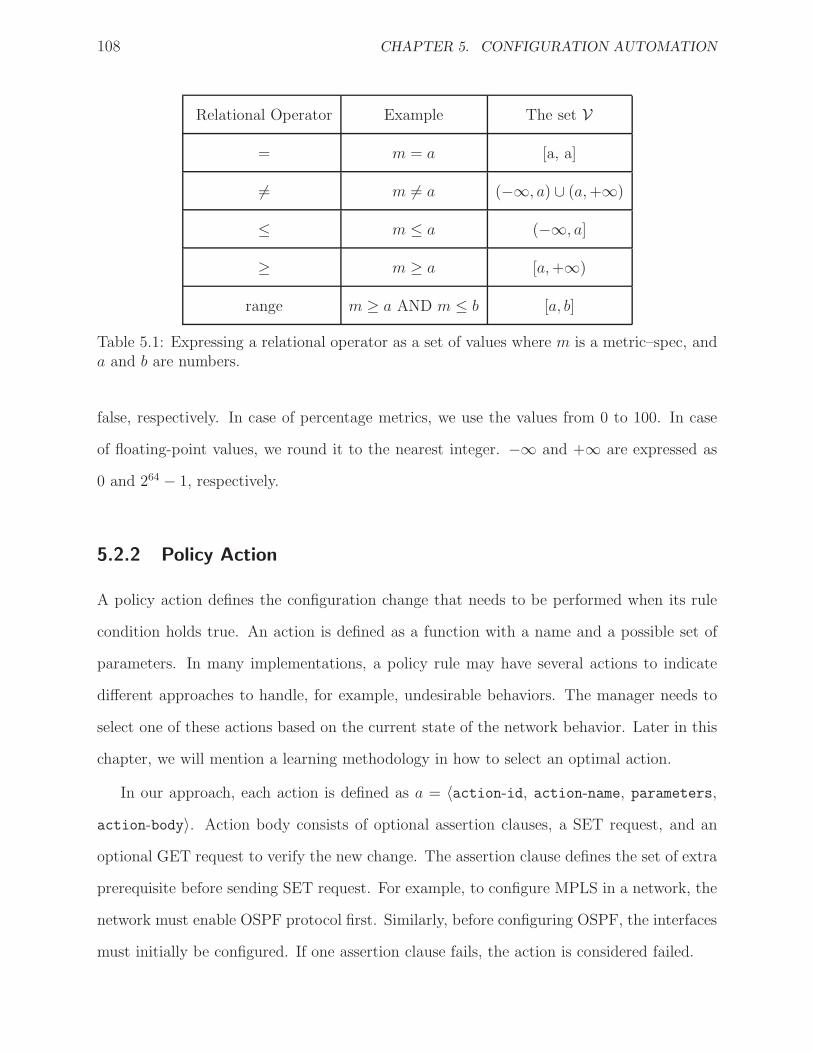
108 CHAPTER 5. CONFIGURATION AUTOMATION
Relational Operator Example The set V
= m = a [a, a]
6= m 6= a (−∞, a) ∪ (a,+∞)
≤ m ≤ a (−∞, a]
≥ m ≥ a [a,+∞)
range m ≥ a AND m ≤ b [a, b]
Table 5.1: Expressing a relational operator as a set of values where m is a metric–spec, anda and b are numbers.
false, respectively. In case of percentage metrics, we use the values from 0 to 100. In case
of floating-point values, we round it to the nearest integer. −∞ and +∞ are expressed as
0 and 264 − 1, respectively.
5.2.2 Policy Action
A policy action defines the configuration change that needs to be performed when its rule
condition holds true. An action is defined as a function with a name and a possible set of
parameters. In many implementations, a policy rule may have several actions to indicate
different approaches to handle, for example, undesirable behaviors. The manager needs to
select one of these actions based on the current state of the network behavior. Later in this
chapter, we will mention a learning methodology in how to select an optimal action.
In our approach, each action is defined as a = 〈action-id, action-name, parameters,
action-body〉. Action body consists of optional assertion clauses, a SET request, and an
optional GET request to verify the new change. The assertion clause defines the set of extra
prerequisite before sending SET request. For example, to configure MPLS in a network, the
network must enable OSPF protocol first. Similarly, before configuring OSPF, the interfaces
must initially be configured. If one assertion clause fails, the action is considered failed.

5.2. POLICY STRUCTURE 109
Using SCL commands, SET request is equivalent to “manage” command and GET re-
quest is equivalent to “verify” command. In case where the action function has a “verify”
command, it must provide a feedback to AutoConf system about the new change. In case
where the action function has no “verify” command, AutoConf will receive the feedback
from the monitor system.
It is desirable that the action function consists of a single “manage” command because
this will allow AutoConf to evaluate the effectiveness of each individual command. For
example, if the action consists of two “manage” commands, then it will be difficult to
understand the impact of these commands; if the “verify” command returns false, is it
because of the first command, the second command or both? By having a single “manage”
command, AutoConf can have more accurate analysis of the actions performed during its
life cycle and can decide the proper order to execute.
5.2.3 Policy Type
There are several types of policies. In this dissertation, we consider only two types of policies:
Configuration policy and Expectation policy [79].
The configuration policies describe how to configure a service where the conditions tell
when and which devices are needed to be configured. List 1 shows an example of a config-
uration policy to set static configuration parameters based on the Service Level Agreement
(SLA) requirements.
At every edge router:
if (Time >= 8am) and (Time <= 11am) and (IPdest = 123.4.5.6) then
setParamters(Transmission = 200Kbps,
PacketLoss = 10,
Delay = 100)
List 1: Configuration Policy Example
Expectation policies describe configuration setup to correct a conflict or a violation and
to ensure the service is running as expected. An example for an expectation policy is shown
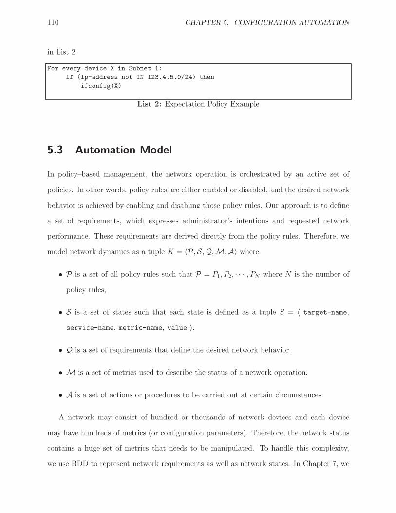
110 CHAPTER 5. CONFIGURATION AUTOMATION
in List 2.
For every device X in Subnet 1:
if (ip-address not IN 123.4.5.0/24) then
ifconfig(X)
List 2: Expectation Policy Example
5.3 Automation Model
In policy–based management, the network operation is orchestrated by an active set of
policies. In other words, policy rules are either enabled or disabled, and the desired network
behavior is achieved by enabling and disabling those policy rules. Our approach is to define
a set of requirements, which expresses administrator’s intentions and requested network
performance. These requirements are derived directly from the policy rules. Therefore, we
model network dynamics as a tuple K = 〈P,S,Q,M,A〉 where
• P is a set of all policy rules such that P = P1, P2, · · · , PN where N is the number of
policy rules,
• S is a set of states such that each state is defined as a tuple S = 〈 target-name,
service-name, metric-name, value 〉,
• Q is a set of requirements that define the desired network behavior.
• M is a set of metrics used to describe the status of a network operation.
• A is a set of actions or procedures to be carried out at certain circumstances.
A network may consist of hundred or thousands of network devices and each device
may have hundreds of metrics (or configuration parameters). Therefore, the network status
contains a huge set of metrics that needs to be manipulated. To handle this complexity,
we use BDD to represent network requirements as well as network states. In Chapter 7, we

5.3. AUTOMATION MODEL 111
show the efficiency of our model by running a set of simulation experiments with different
network topologies.
To optimize the selection of action based on the current network state and requirement
set, we implement RL with Dyna-Q algorithm. In this section, we first show how to model
network requirements using BDD. Then we show how to automate action selection by using
RL technique.
5.3.1 Policy Representation
The management system requires a set of requirements to be achieved and maintained during
the life cycle of a network. These requirements are actually derived from the policy rules. If
a policy rule represents a violation, then the negation of the policy conditions constructs a
requirement as shown in Figure 5.2. Let us consider again the following policy: “if there is a
network interface in Subnet 1 that does not belong to the network address 10.1.1.0/24 then
invoke the action ifconfig()”. The system checks the Subnet 1’s repository. If the repository
indicates that there are two routers (say R1 and R2) and each with two interfaces (say e0/0
and s0/0), then the system will create four requirements.
High-level Policy
Rules
AutoConf
Low-level
Requirements
Figure 5.2: High-level policy rules are translated to low-level requirements
Before we list these requirements, we need to define a requirement formally. A require-
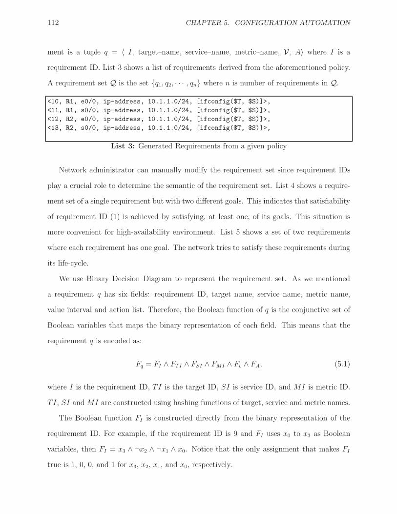
112 CHAPTER 5. CONFIGURATION AUTOMATION
ment is a tuple q = 〈 I, target–name, service–name, metric–name, V, A〉 where I is a
requirement ID. List 3 shows a list of requirements derived from the aforementioned policy.
A requirement set Q is the set {q1, q2, · · · , qn} where n is number of requirements in Q.
<10, R1, e0/0, ip-address, 10.1.1.0/24, [ifconfig($T, $S)]>,
<11, R1, s0/0, ip-address, 10.1.1.0/24, [ifconfig($T, $S)]>,
<12, R2, e0/0, ip-address, 10.1.1.0/24, [ifconfig($T, $S)]>,
<13, R2, s0/0, ip-address, 10.1.1.0/24, [ifconfig($T, $S)]>,
List 3: Generated Requirements from a given policy
Network administrator can manually modify the requirement set since requirement IDs
play a crucial role to determine the semantic of the requirement set. List 4 shows a require-
ment set of a single requirement but with two different goals. This indicates that satisfiability
of requirement ID (1) is achieved by satisfying, at least one, of its goals. This situation is
more convenient for high-availability environment. List 5 shows a set of two requirements
where each requirement has one goal. The network tries to satisfy these requirements during
its life-cycle.
We use Binary Decision Diagram to represent the requirement set. As we mentioned
a requirement q has six fields: requirement ID, target name, service name, metric name,
value interval and action list. Therefore, the Boolean function of q is the conjunctive set of
Boolean variables that maps the binary representation of each field. This means that the
requirement q is encoded as:
Fq = FI ∧ FTI ∧ FSI ∧ FMI ∧ Fv ∧ FA, (5.1)
where I is the requirement ID, TI is the target ID, SI is service ID, and MI is metric ID.
TI, SI and MI are constructed using hashing functions of target, service and metric names.
The Boolean function FI is constructed directly from the binary representation of the
requirement ID. For example, if the requirement ID is 9 and FI uses x0 to x3 as Boolean
variables, then FI = x3 ∧ ¬x2 ∧ ¬x1 ∧ x0. Notice that the only assignment that makes FI
true is 1, 0, 0, and 1 for x3, x2, x1, and x0, respectively.

5.3. AUTOMATION MODEL 113
<1, R1, interface, s0/0, 1, [enable_interface($T, $M)]>
<1, R1, interface, s0/1, 1, [enable_interface($T, $M)]>
List 4: Single requirement with two different goals
<10, R1, interface, s0/0, 1, [enable_interface($T, $M)]>
<20, R1, interface, s0/1, 1, [enable_interface($T, $M)]>
List 5: Two different requirements
Target ID can be a single ID to indicate that the requirement q is applied to a single
target or a domain ID to indicate that the requirement q is applied to a group of devices.
In case of a domain ID, the satisfiability of this requirement is achieved if there is at least
one target satisfies the requirement. Also, Target ID can be “any” to indicate that the
requirement q is applied to any target defined in a network. Therefore, the Boolean function
of FDI is
FTI =
F (hash(target name)) for a single target∨
k∈D F (k) for a domain target
true for any target
The variable D is the set of targets (or devices) in a domain based on CSM parent–child
relationships. For example, the metric 〈R1, s0/0, PacketLoss〉 is formulated as FH(“R1”) ∧
FH(“s0/0”) ∧ F
H(“PacketLoss”) where H() is a hash function.
The Boolean function Fv is constructed by the disjunction of powers of two values span-
ning the interval V. For example, [3, 7] = [3, 3] ∪ [4, 7] and can be encoded (using 3 bits) as
Fv = (¬x12 ∧ x11 ∧ x10)∨
x12 assuming that x10 to x12 are used to encode Fv.
The Boolean function FA is given as
FA =
m∨
k=1
Fak
where A = {ak, k = 1, 2, · · · , m}, ak is an action ID, and Fak is constructed directly from
the binary representation of the action ID of ak.
Now, let Q = {q1, q2, · · · , qM} be a set of M requirements. We represent Q as a Boolean
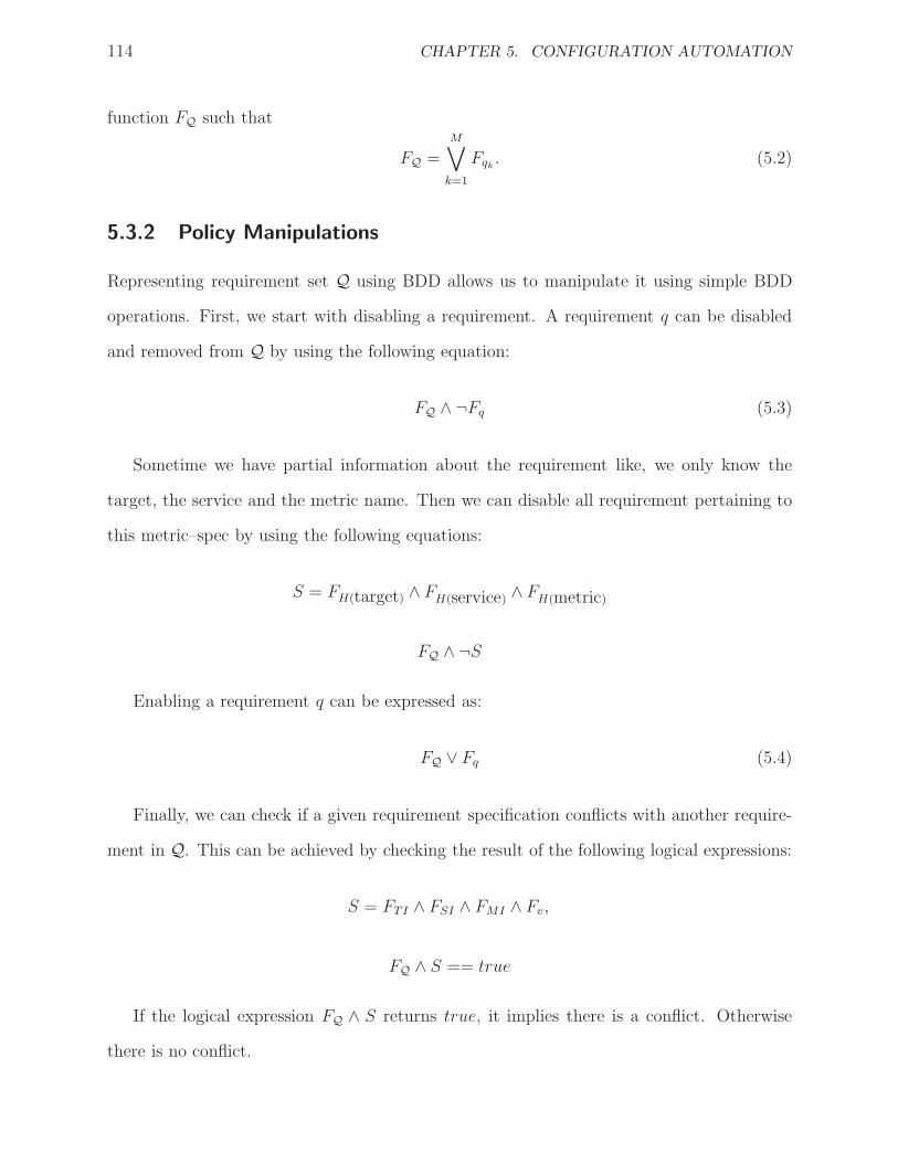
114 CHAPTER 5. CONFIGURATION AUTOMATION
function FQ such that
FQ =M∨
k=1
Fqk . (5.2)
5.3.2 Policy Manipulations
Representing requirement set Q using BDD allows us to manipulate it using simple BDD
operations. First, we start with disabling a requirement. A requirement q can be disabled
and removed from Q by using the following equation:
FQ ∧ ¬Fq (5.3)
Sometime we have partial information about the requirement like, we only know the
target, the service and the metric name. Then we can disable all requirement pertaining to
this metric–spec by using the following equations:
S = FH(target) ∧ FH(service) ∧ F
H(metric)
FQ ∧ ¬S
Enabling a requirement q can be expressed as:
FQ ∨ Fq (5.4)
Finally, we can check if a given requirement specification conflicts with another require-
ment in Q. This can be achieved by checking the result of the following logical expressions:
S = FTI ∧ FSI ∧ FMI ∧ Fv,
FQ ∧ S == true
If the logical expression FQ ∧ S returns true, it implies there is a conflict. Otherwise
there is no conflict.

5.3. AUTOMATION MODEL 115
5.3.3 System State Representation
As we mentioned, network behavior is described by using a set of metrics. The current values
of these metrics define the current network operation. We assume that the monitor system
provides to the AutoConf system the following information when it reports the status of a
metric:
metric state m ::= <target name, service name, metric name, observed value>.
First, let Mt be a collection of metric states collected at time t. At time t0, the network
state S is clearly equivalent to Mt0 . For time t > t0, the network state is updated based on
the current set Mt and the previous network state Sold. Let t1 and t2 be two consecutive
times such that t2 > t1. Let St1 be the network state at time t1 and let Mt2 be the set of
states that have been received from the monitor system. Then the network state at time t2
can be expressed as:
St2 = Mt2 ∪[
St1 −(
St1 ∩M ′t2
)]
. (5.5)
where M ′ is constructed by setting each metric state m ∈ M to “any”.
Next, we show how to represent a network state using BDD. First, we encode each metric
state m as:
Fm = FTI ∧ FSI ∧ FMI ∧ Fv.
Second, we compute FM as:
FM =K∨
k=1
Fmk, (5.6)
where mk ∈ M . Last, the network state can be expressed using Equation 5.5 as:
FS = FM ∨ [FSold∧ ¬ (FSold
∧ FM ′)] . (5.7)
where FM ′ = τ(FM , Fv) and τ() is the mask function as given in Chapter 4.
AutoConf system compares the current network state with the requirement set Q to
determine whether it needs to take an action or not. Based on the current network state,
the requirement set Q is divided into the following subsets:
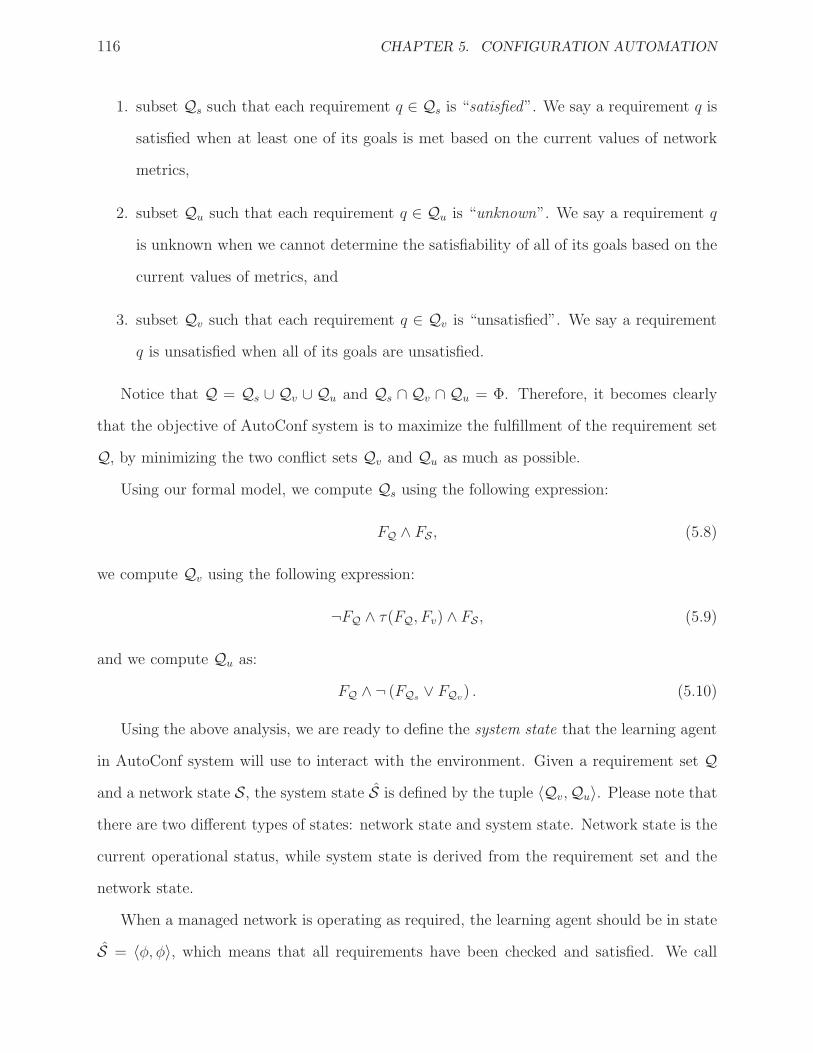
116 CHAPTER 5. CONFIGURATION AUTOMATION
1. subset Qs such that each requirement q ∈ Qs is “satisfied”. We say a requirement q is
satisfied when at least one of its goals is met based on the current values of network
metrics,
2. subset Qu such that each requirement q ∈ Qu is “unknown”. We say a requirement q
is unknown when we cannot determine the satisfiability of all of its goals based on the
current values of metrics, and
3. subset Qv such that each requirement q ∈ Qv is “unsatisfied”. We say a requirement
q is unsatisfied when all of its goals are unsatisfied.
Notice that Q = Qs ∪ Qv ∪ Qu and Qs ∩ Qv ∩ Qu = Φ. Therefore, it becomes clearly
that the objective of AutoConf system is to maximize the fulfillment of the requirement set
Q, by minimizing the two conflict sets Qv and Qu as much as possible.
Using our formal model, we compute Qs using the following expression:
FQ ∧ FS , (5.8)
we compute Qv using the following expression:
¬FQ ∧ τ(FQ, Fv) ∧ FS , (5.9)
and we compute Qu as:
FQ ∧ ¬ (FQs∨ FQv
) . (5.10)
Using the above analysis, we are ready to define the system state that the learning agent
in AutoConf system will use to interact with the environment. Given a requirement set Q
and a network state S, the system state S is defined by the tuple 〈Qv,Qu〉. Please note that
there are two different types of states: network state and system state. Network state is the
current operational status, while system state is derived from the requirement set and the
network state.
When a managed network is operating as required, the learning agent should be in state
S = 〈φ, φ〉, which means that all requirements have been checked and satisfied. We call

5.3. AUTOMATION MODEL 117
this state the goal state. When one or more requirements are unsatisfied, the set Qv 6= φ or
FQv6= false. The learning agent then decodes FQv
to extract the action list along with the
metric specifications: target name, service name and metric name. Therefore, the objective
of the learning agent is to move efficiently the system state from undesired state to the goal
state by constructing a plan adaptively. The plan describes the optimal set of actions to
reach the goal state. The following section shows how to build up this plan.
5.3.4 Action Selection
We model our system using a finite state machine. In this context, the management system
encounters a set of actions extracted from Qv and Qu and must decide the next action to
be performed at each state. This section shows how the management system learns effective
decision-making policies when it interacts with the managed network.
As we mentioned in Chapter 2, an agent in RL learns optimal policy by interacting with
its environment. In every time step t, the learning agent performs the following tasks:
• observing the environment current state st at time t,
• determining the next action (using for example ǫ-greedy algorithm) from a list of legal
actions at state s,
• executing the action and observing the new state st+1, and
• receiving a reward rt.
The main objective of RL algorithm is to maximize the cumulative reward it receives.
This can be achieved by estimating action-value function Q(s, a) which assigns a value when
taking action a at state s. In Q-learning, Q(s, a) is estimated using the following equation:
Q(st, at)← Q(st, at) + α
[
rt + γmaxat+1
Q(st+1, at+1)−Q(st, at)
]
(5.11)
Here α is a learning rate factor, γ is a discount factor between 0 and 1 expressing how
strongly present value relies on future rewards, and rt is the immediate reward. The Q(s, a)

118 CHAPTER 5. CONFIGURATION AUTOMATION
measures how good it is for the management system to execute action a in a given state s.
Several powerful theorems guarantee that Q-learning converges with probability of 1. Dyna-
Q algorithm 4 proposed by Sutton supports system model and management policy and it is
closely related to the adaptive method we develop. The algorithm estimates Q(s, a) using
Equation 5.11. The algorithm starts by observing and analyzing the current network state
using Equations 5.8 to Equation 5.9. Then it goes into infinite loop. In the loop, it checks
if the system state is at the goal state. If so, the algorithm observes and analyzes the next
network state. If not, the algorithm invokes ǫ−greedy function to determine the next action
to be executed. In ǫ–greedy, the agent selects the highest Q value most of the time (i.e.,
with probability of 1− ǫ).
The effect of an action is analyzed by observing the new network state and rewarding it
as a result. Using this information, the algorithm updates the action-state values and adds
this information to the system model.
5.3.5 The Reward Function
The reward signal is used to formalize the learning agent’s ultimate goal; steering the network
from undesired network operational state to a desired network operational state. The state-
action function expressed in Equation 5.11 defines how good it is for the learning agent to
perform a given action in a given state. As such, the learning agent tries to maximize the
expected reward value in a long run. Therefore, it is critical to setup a reward value that is
truly directing the management system to handle any performance or configuration issues.
The simplest approach is to reward the agent for any transition it makes. However,
this may deviate the system from more acceptable state to less acceptable state. Another
solution, which has been proposed in [91, 7], is to assign each state with a reward based on
the desirability of each state. The desirability of a state is measured by two factors. The
first factor is the cumulative weight for each metric involved in that state. The metric’s
weight is used to indicate its importance. The second factor depends on the current values
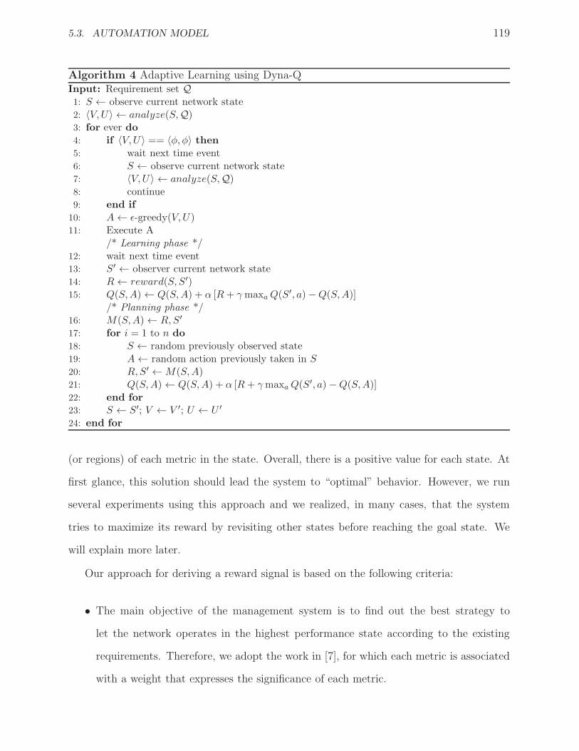
5.3. AUTOMATION MODEL 119
Algorithm 4 Adaptive Learning using Dyna-QInput: Requirement set Q1: S ← observe current network state2: 〈V,U〉 ← analyze(S,Q)3: for ever do4: if 〈V,U〉 == 〈φ, φ〉 then5: wait next time event6: S ← observe current network state7: 〈V,U〉 ← analyze(S,Q)8: continue9: end if
10: A← ǫ-greedy(V,U)11: Execute A
/* Learning phase */12: wait next time event13: S′ ← observer current network state14: R← reward(S, S′)15: Q(S,A)← Q(S,A) + α [R+ γmaxaQ(S′, a)−Q(S,A)]
/* Planning phase */16: M(S,A)← R,S′
17: for i = 1 to n do
18: S ← random previously observed state19: A← random action previously taken in S
20: R,S′ ←M(S,A)21: Q(S,A)← Q(S,A) + α [R+ γmaxaQ(S′, a)−Q(S,A)]22: end for
23: S ← S′; V ← V ′; U ← U ′
24: end for
(or regions) of each metric in the state. Overall, there is a positive value for each state. At
first glance, this solution should lead the system to “optimal” behavior. However, we run
several experiments using this approach and we realized, in many cases, that the system
tries to maximize its reward by revisiting other states before reaching the goal state. We
will explain more later.
Our approach for deriving a reward signal is based on the following criteria:
• The main objective of the management system is to find out the best strategy to
let the network operates in the highest performance state according to the existing
requirements. Therefore, we adopt the work in [7], for which each metric is associated
with a weight that expresses the significance of each metric.
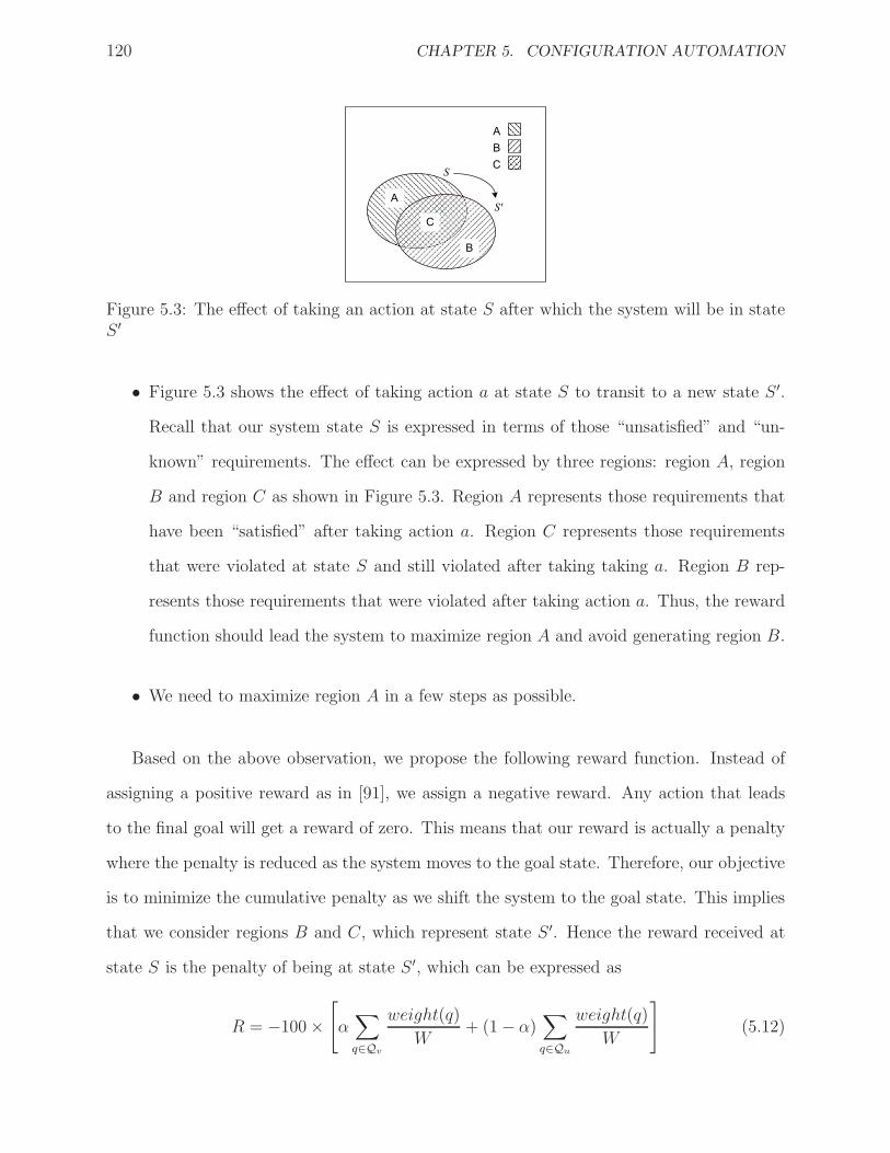
120 CHAPTER 5. CONFIGURATION AUTOMATION
S'
S
A
B
C
A
B
C
Figure 5.3: The effect of taking an action at state S after which the system will be in stateS ′
• Figure 5.3 shows the effect of taking action a at state S to transit to a new state S ′.
Recall that our system state S is expressed in terms of those “unsatisfied” and “un-
known” requirements. The effect can be expressed by three regions: region A, region
B and region C as shown in Figure 5.3. Region A represents those requirements that
have been “satisfied” after taking action a. Region C represents those requirements
that were violated at state S and still violated after taking taking a. Region B rep-
resents those requirements that were violated after taking action a. Thus, the reward
function should lead the system to maximize region A and avoid generating region B.
• We need to maximize region A in a few steps as possible.
Based on the above observation, we propose the following reward function. Instead of
assigning a positive reward as in [91], we assign a negative reward. Any action that leads
to the final goal will get a reward of zero. This means that our reward is actually a penalty
where the penalty is reduced as the system moves to the goal state. Therefore, our objective
is to minimize the cumulative penalty as we shift the system to the goal state. This implies
that we consider regions B and C, which represent state S ′. Hence the reward received at
state S is the penalty of being at state S ′, which can be expressed as
R = −100×
[
α∑
q∈Qv
weight(q)
W+ (1− α)
∑
q∈Qu
weight(q)
W
]
(5.12)
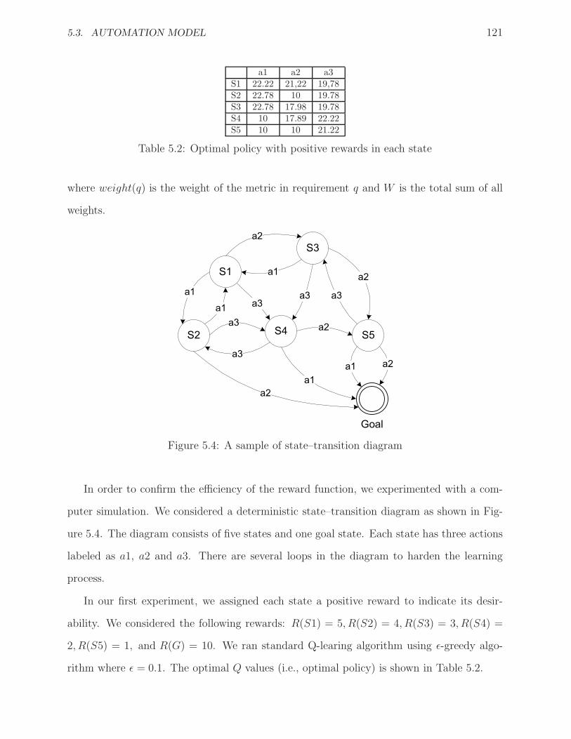
5.3. AUTOMATION MODEL 121
a1 a2 a3S1 22.22 21,22 19,78S2 22.78 10 19.78S3 22.78 17.98 19.78S4 10 17.89 22.22S5 10 10 21.22
Table 5.2: Optimal policy with positive rewards in each state
where weight(q) is the weight of the metric in requirement q and W is the total sum of all
weights.
S1
S2 S5S4
S3
Goal
a2
Figure 5.4: A sample of state–transition diagram
In order to confirm the efficiency of the reward function, we experimented with a com-
puter simulation. We considered a deterministic state–transition diagram as shown in Fig-
ure 5.4. The diagram consists of five states and one goal state. Each state has three actions
labeled as a1, a2 and a3. There are several loops in the diagram to harden the learning
process.
In our first experiment, we assigned each state a positive reward to indicate its desir-
ability. We considered the following rewards: R(S1) = 5, R(S2) = 4, R(S3) = 3, R(S4) =
2, R(S5) = 1, and R(G) = 10. We ran standard Q-learing algorithm using ǫ-greedy algo-
rithm where ǫ = 0.1. The optimal Q values (i.e., optimal policy) is shown in Table 5.2.
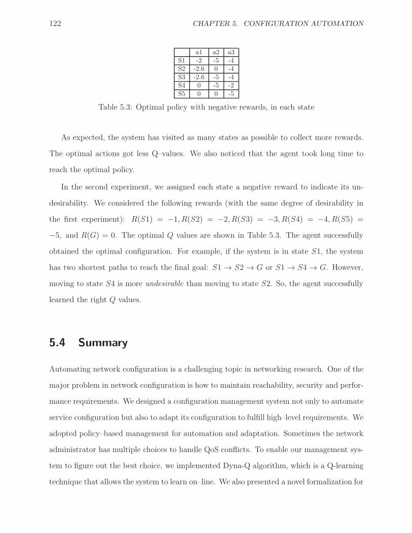
122 CHAPTER 5. CONFIGURATION AUTOMATION
a1 a2 a3S1 -2 -5 -4S2 -2.6 0 -4S3 -2.6 -5 -4S4 0 -5 -2S5 0 0 -5
Table 5.3: Optimal policy with negative rewards, in each state
As expected, the system has visited as many states as possible to collect more rewards.
The optimal actions got less Q–values. We also noticed that the agent took long time to
reach the optimal policy.
In the second experiment, we assigned each state a negative reward to indicate its un-
desirability. We considered the following rewards (with the same degree of desirability in
the first experiment): R(S1) = −1, R(S2) = −2, R(S3) = −3, R(S4) = −4, R(S5) =
−5, and R(G) = 0. The optimal Q values are shown in Table 5.3. The agent successfully
obtained the optimal configuration. For example, if the system is in state S1, the system
has two shortest paths to reach the final goal: S1 → S2 → G or S1→ S4 → G. However,
moving to state S4 is more undesirable than moving to state S2. So, the agent successfully
learned the right Q values.
5.4 Summary
Automating network configuration is a challenging topic in networking research. One of the
major problem in network configuration is how to maintain reachability, security and perfor-
mance requirements. We designed a configuration management system not only to automate
service configuration but also to adapt its configuration to fulfill high–level requirements. We
adopted policy–based management for automation and adaptation. Sometimes the network
administrator has multiple choices to handle QoS conflicts. To enable our management sys-
tem to figure out the best choice, we implemented Dyna-Q algorithm, which is a Q-learning
technique that allows the system to learn on–line. We also presented a novel formalization for

5.4. SUMMARY 123
modeling configuration and expectation policies in order to have a compact representation
and to enable us to use Dyna-Q with large–sized networks.


Chapter 6
Implementation
AutoConf system is mainly implemented using the Erlang language along with C programs
that are linked to the Erlang Subsystem. In this chapter, we provide a brief overview of
the Erlang language and we then present in detail the overall architecture of the AutoConf
system. Since AutoConf relies on the SCL language, we also present the SCL grammar. Fi-
nally, we discuss the implementation of network configuration change, network configuration
verification and network configuration automation.
6.1 Erlang Language
Erlang [3] is a concurrent functional programming language that supports real-time and
fault-tolerance distributed systems. It has been used in writing many critical applications
such as the AXD 301 ATM switch1 [13].
An Erlang program consists of a set of modules. Each module basically contains a list
of function definitions. Each function consists of a set of Erlang expressions. A function,
which has a name fun name defined in the module mod name with arity N , is often denoted
as mod name:fun name/N. List 6 shows a sample Erlang module called echo which exports
1The software was consisting of over half a million lines of Erlang code.
125

126 CHAPTER 6. IMPLEMENTATION
two functions: start/0 and loop/0. The function start/0 spawns a new process which
will be responsible to execute echo:loop/0 function in parallel with the calling function.
Each process has a message queue to store the incoming messages. Erlang has asynchronous
communication mechanism where any process can send a message to any other process by
using ! operator. The later process can inspect its mailbox by the receive statement. A
sequence of patterns can be specified to read specific messages from the mailbox. When
reading a message, a process is suspended until a matching message arrives or timeout
occurs.
Erlang language has a huge library called OTP (Open Telecom Platform). OTP is a
programming platform that provides ready–to–use components (libraries) and services such
as:
• Distributed database system called Mnesia. Mnesia was designed to provide concur-
rent, soft real–time system with high–availability requirement. It supports database
transactions, data indexing, and relational queries.
• Fast key–value lookups of potentially complex data [31].
• Efficient set of algorithms for directed graph and directed acyclic graph (DAG).
-module(echo).
-export([start/0, loop/0]).
start() ->
spawn(echo, loop, []).
loop() ->
receive
{From, Message} ->
From ! Message,
loop()
end.
List 6: Erlang module
6.2. OVERALL ARCHITECTURE 127
• XML, SSH and encryption libraries that can be used to implement NETCONF protocol
at client side.
• An LALR-1 parser generator for Erlang called yecc similar to yacc.
• Port driver that links Erlang program with other programs written in different lan-
guages such as C, C++ and Java.
For more information about the language, the reader may refer to [3].
6.2 Overall Architecture
The overall architecture of AutoConf system utilizing our proposed framework, as described
in section 3.2, is depicted in Figure 6.1. Network administrators perform device configuration
by accessing SCL-enabled console manager. The console manager provides interactive text-
based interface to read manager commands or SCL files to be executed. While executing
commands, the console manager may require to query Domain Knowledge Base (DKB) to
retrieve some specific CSM predicates.
AutoConf is a fault-tolerant system since it is expected to run forever. AutoConf applica-
tion consists mainly of AutoConf Supervisor, SSH engine, and Database Engine. AutoConf
supervisor is responsible to launch and monitor BDD processes, policy engine and Device
Supervisor. BDD processes are responsible to run an exteranl BDD package and link that
package with the Erlang system. A BDD package is linked to the Erlang system using Er-
lang port interface instead of dynamically linked into the Erlang system. Although dynamic
linkage is the fastest way of calling C functions from Erlang, it is least safe because a crash
in BDD package brings AutoConf down too.
Device Supervisor is responsible to launch and monitor the device manager and a set
of device processes. Each device process is associated with a physical network device, and
when it launches, it tries to establish a persistent NETCONF session with that physical

128 CHAPTER 6. IMPLEMENTATION
SSH engine
AutoConf Applicaton
Database Engine
Device
Supervisor
Device Manager
Device
Process
Device
Process
Device
Process
Netconf-enabled
Network Devices
BDD Engine
Console Manager
NETCONF module
AutoConf
Executer
Inference Engine
Local
DB
KDB
SCL Compiler
AutoConf
Supervisor
Policy
Communication Network
Figure 6.1: AutoConf management architecture
device. To enable AutoConf to communicate to all managed devices at once, it is expected
that all managed devices have the same authentication information, and therefore the de-
vice supervisor prompts for password authentication only once and uses that password to
authenticate with all NETCONF-enabled network devices. If a device process is killed due
to a connection loss between AutoConf and a physical network device, the device supervisor
keeps trying to connect to that device for a period of one hour before it gives up.
Policy engine is responsible to handle network requirements as well as network states
received from a monitor subsystem (not shown in the figure). Policy actions, which are
required to be executed, are sent to the AutoConf executer. It is worth mentioning that the
policy engine acts as a policy decision point (PDP) as described in IETF COPS architecture

6.2. OVERALL ARCHITECTURE 129
(RFC 3198). The device manager acts as a policy enforcement point (PEP), while device
processes act as effectors (E’s).
All engines are linked to the AutoConf executer. AutoConf Executer is a set of Erlang
modules to performs severals tasks. One task is to execute the user commands. Another
task is to provide a unified interface to the database engine.
Figure 6.2 shows process hierarchy of AutoConf application in the Erlang system. Au-
toConf application runs Mnesia, Crypto, and SSH applications as shown on the left–hand
side. AutoConf’s main process has process ID (PID) < 0.38.0 > and creates a control pro-
cess with PID < 0.39.0 >. This control process creates Autoconf supervisor(autoconf sup)
which, in turn, creates two BDD engines buddy and rsm, policy engine and device supervi-
sor (device sup) engine. As shown, there are four device processes: rtr01, rtr02, rtr03 and
rtr04. Each device process establishes a persistent NETCONF session with its associated
network device. Notice that the name of a device process is the same name as in CSM’s
device concept.
Figure 6.2: AutoConf Application running in Erlang system
The architecture involves different kind of users to build NETCONF-enabled automated
system. One user is responsible to write the appropriate data models for the network
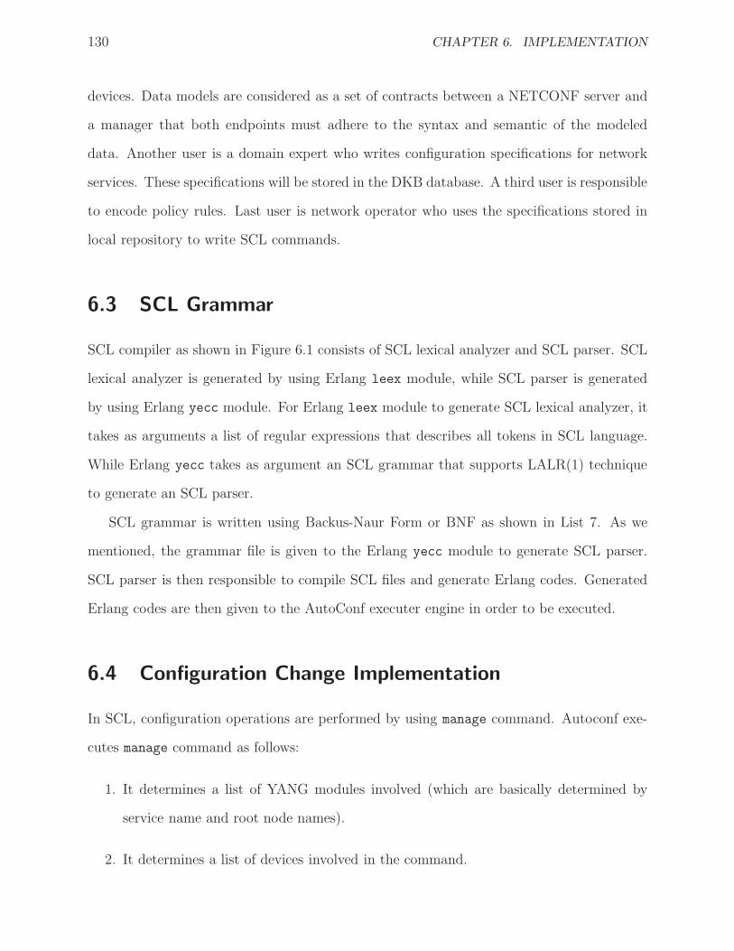
130 CHAPTER 6. IMPLEMENTATION
devices. Data models are considered as a set of contracts between a NETCONF server and
a manager that both endpoints must adhere to the syntax and semantic of the modeled
data. Another user is a domain expert who writes configuration specifications for network
services. These specifications will be stored in the DKB database. A third user is responsible
to encode policy rules. Last user is network operator who uses the specifications stored in
local repository to write SCL commands.
6.3 SCL Grammar
SCL compiler as shown in Figure 6.1 consists of SCL lexical analyzer and SCL parser. SCL
lexical analyzer is generated by using Erlang leex module, while SCL parser is generated
by using Erlang yecc module. For Erlang leex module to generate SCL lexical analyzer, it
takes as arguments a list of regular expressions that describes all tokens in SCL language.
While Erlang yecc takes as argument an SCL grammar that supports LALR(1) technique
to generate an SCL parser.
SCL grammar is written using Backus-Naur Form or BNF as shown in List 7. As we
mentioned, the grammar file is given to the Erlang yecc module to generate SCL parser.
SCL parser is then responsible to compile SCL files and generate Erlang codes. Generated
Erlang codes are then given to the AutoConf executer engine in order to be executed.
6.4 Configuration Change Implementation
In SCL, configuration operations are performed by using manage command. Autoconf exe-
cutes manage command as follows:
1. It determines a list of YANG modules involved (which are basically determined by
service name and root node names).
2. It determines a list of devices involved in the command.
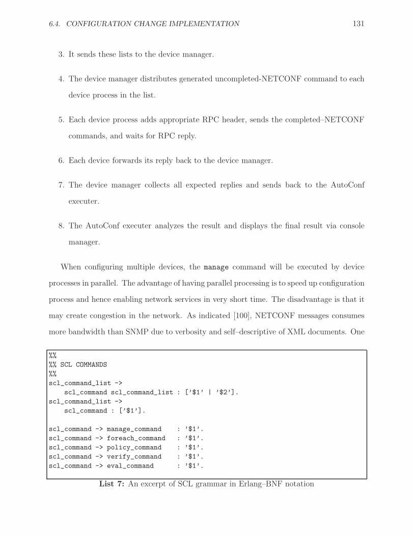
6.4. CONFIGURATION CHANGE IMPLEMENTATION 131
3. It sends these lists to the device manager.
4. The device manager distributes generated uncompleted-NETCONF command to each
device process in the list.
5. Each device process adds appropriate RPC header, sends the completed–NETCONF
commands, and waits for RPC reply.
6. Each device forwards its reply back to the device manager.
7. The device manager collects all expected replies and sends back to the AutoConf
executer.
8. The AutoConf executer analyzes the result and displays the final result via console
manager.
When configuring multiple devices, the manage command will be executed by device
processes in parallel. The advantage of having parallel processing is to speed up configuration
process and hence enabling network services in very short time. The disadvantage is that it
may create congestion in the network. As indicated [100], NETCONF messages consumes
more bandwidth than SNMP due to verbosity and self–descriptive of XML documents. One
%%
%% SCL COMMANDS
%%
scl_command_list ->
scl_command scl_command_list : [’$1’ | ’$2’].
scl_command_list ->
scl_command : [’$1’].
scl_command -> manage_command : ’$1’.
scl_command -> foreach_command : ’$1’.
scl_command -> policy_command : ’$1’.
scl_command -> verify_command : ’$1’.
scl_command -> eval_command : ’$1’.
List 7: An excerpt of SCL grammar in Erlang–BNF notation

132 CHAPTER 6. IMPLEMENTATION
solution is to encapsulate manage with foreach command so that it iterates over devices. In
this case, foreach produces a series of manage commands that will be executed sequentially.
6.5 Configuration Verification Implementation
Configuration verification as mentioned in section 4.4 relies on a formal model, which is
BDD. In our implementation, we use 104 bits to encode the packet header plus 8 bits to
encode the action field. In case of routing policy and firewall policy, the action field is used
to encode a device interface. This implies that the maximum of number of interfaces is 128
(since one bit is used for direction).
In SCL, a verification rule is represented by using either policy or verify commands.
The execution path of these commands is similar to the manage command as described in
the previous section.
6.6 Configuration Automation Implementation
Configuration Automation is implemented inside the policy engine. This engine uses RSM
(Requirement and State BDD Module) engine to encode requirements and network states.
All equations discussed in Chapter 5 use 20 bits to encode Requirement ID, 45 bits to encode
metric specification (target name + service name + metric name), 64 bits to encode value
range and one bit to encode value type (0 numberic value, 1 IP address). Thus, the total
number of bits is 130 bits.
The policy engine is acting like an event-handler server. It waits for an event either from
a monitor or from a timer, to begin its management cycle. In this cycle, the engine performs
Algorithm 4 (as described in Chapter 5). If it decides to execute an action, then it will send
a notification to AutoConf Executer to run SCL function. The notification carries the SCL
function name along with a list of arguments.

6.7. SUMMARY 133
6.7 Summary
In this chapter, we present an overview of the overall architecture of AutoConf system.
Then we present how we developed the SCL language. Finally, we shed some lights on how
AutoConf performs configuration operations, verification, and automation.


Chapter 7
Experimental and Evaluation Results
This chapter presents a set of experiments to evaluate AutoConf flexibility and its per-
formance. To evaluate its scalability, we run a set of simulations with different network
sizes.
7.1 Experimental Setup
The setup of our experiments consists of a hypervisor machine running VMware ESXi version
4.1. The machine that hosts the VMware is equipped with an Intel Pentium dual-core CPU
running at 2.8 GHz, a memory RAM of size 4GB, and two SATA hard-drives. On the top of
VMware’s hypervisor, there are seven virtual machines each running CentOS 6.2 with Linux
kernel 2.6.32. Four virtual machines are acting as routers. The routing software installed
in these machines is Quagga version 0.99. Quagga supports most IP routing protocols such
RIPv1, RIPv2, OSPF, and BGP. Two virtual machines are used as two end hosts. And the
last one is used as an administrator machine which runs our tool AutoConf.
AutoConf assumes that managed devices are implementing NETCONF protocol and
YANG data model (RFCs 4741, 6241 and 6020). There are several tools that supports
NETCONF protocol. Throughout our dissertation, we investigated three tools: EnSuite,
135

136 CHAPTER 7. EXPERIMENTAL AND EVALUATION RESULTS
ConfD and Yuma NETCONF server.
EnSuite [59], ConfD [86] and Yuma [102] are network management suits. They consists
of a NETCONF agent (or NETCONF server), a NETCONF manager and a set of extension
libraries and utilities such as YANG parser. The followings give a brief description for each
suite.
EnSuite is an open source framework implemented in Python. It consists of YencaP server
(NETCONF agent), YencaP manager and YANG parser called jYANG. YencaP server is an
extensible server compliant to NETCONF protocol 1.0. YencaP manager is a NETCONF
client application that sends queries and receives responses with any NETCONF-compliant
server. It acts as HTTPS server where a user can establish HTTPS sessions. There is a
one to one mapping between HTTPS and NETCONF sessions. Once an HTTPS session
is established and subsequently connected to NETCONF Server, YencaP displays the man-
agement information in graphical interface (as Java Applet) supported by that server in a
tree structure fashion. A user can navigate through the tree and perform GET and SET
operations, where permissible, on any node in the tree.
There are several disadvantages of YencaP server. First, it has a limited support for
the NETCONF protocol. It does not support NETCONF protocol 1.1, NETCONF notifi-
cations, and partial locks. Second, the last updated version was published in 2010 before
standardizing the YANG data model. Thus, jYang is based on a draft version. Third,
our experimental data shows that YencaP does not check the correctness of the uploaded
data. In other words, YencaP does not automatically check the configuration data sent by
a manager.
ConfD is a commercial framework developed by Tail-f that implements the NETCONF
protocol and YANG data model. ConfD is basically a management platform that can be
installed on managed devices and run as a regular Unix daemon. ConfD can act as a
NETCONF server, an SNMP agent, a Web server or as CLI. It also contains a built-in XML
configuration database.

7.1. EXPERIMENTAL SETUP 137
In ConfD, each managed object (such network interfaces, DNS service, or OSPF service)
is associated with a software application that binds YANG content to the managed object.
This software, which runs as a regular UNIX daemon, implements the specific behavior as
defined by the YANG module statements. ConfD process and managed object processes
are connected via TCP/IP Socket interface. Moreover, ConfD allows NETCONF managers
to send NETCONF messages via TCP without SSH. This is a very useful feature for agent
developers to easily debug the software and trace the packets exchanged between ConfD and
NETCONF managers.
Yuma initially was an open source framework implemented in C language. The last
version developed as an open source was 2.2.5. It consists of netconfd (NETCONF server),
yangcli (NETCONF client) and YANG parser called pYang. In the following paragraphs,
we provide detailed differences between Yuma and ConfD
• ConfD and Yuma have different architectures. As we mentioned, there is a dedicated
process called “Confd” that implements the NETCONF protocol at the server side.
Each agent software is a separate process that communicates to “confd” using TCP
sockets. Yuma server is always a single process because the agent software is linked
to the NETCONF server as a shared library. Therefore, Yuma server is more efficient
than ConfD in terms of performance. However, ConfD is more reliable than Yuma,
because if an agent software has crashed due to bugs in coding, only the agent process
would be crashed. It would not affect the ConfD process and the other agent processes.
In Yuma, if the agent software has crashed, the whole process would be collapsed.
• Both Yuma and ConfD servers can be tuned and configured by editing their configu-
ration files. ConfD configuration file is an XML file, while Yuma configuration file is
a YANG file. Eventually, Yuma has been developed based on YANG technology. All
features are added as YANG module, including NETCONF protocol description itself.
This makes Yuma package more flexible and extensible than ConfD.

138 CHAPTER 7. EXPERIMENTAL AND EVALUATION RESULTS
• Before running Yuma NETCONF server, all shared libraries (agent programs) should
be stored in a specific directory as well as their YANG data models. The server
checks these directories and loads these shared libraries automatically. A manager
can load a shared library manually without shutting down the server. In ConfD, the
ConfD process should be executed first, then other agent processes can be executed
individually.
• Both Yuma and ConfD support Command-Line Interface to manage agents. They
both supports auto-completion feature like Cisco CLI. In Yuma, the manager must
first establish NETCONF session using connect command. Then CLI provides a set
of commands to query, create, modify, and delete configuration variables. Based on
our empirical work with Yuma NETCONF client, a manager cannot send an XML
document to the NETCONF server as in ConfD package. Moreover, ConfD has the
capability to auto-generate a web site to build a web-based interface as an alternative
north-bound interface.
• Yuma and ConfD suites provide a set of API to help agent developer to bind YANG
content with managed object content. In Yuma, the API is a set of C functions, while in
ConfD the API is written in C and Java. Yuma provides a very useful tool to generate
a template software tailored based on YANG modules. This will eventually reduce the
developing time dramatically. On the other hand, ConfD requires some modifications
to YANG modules in order for agent software to be able to handle YANG contents.
The last open source version of Yuma was 2.2.5. This version supports NETCONF protocol
1.0 and 1.1, all NETCONF standard capabilities (like confirm, validate, xpath, etc), YANG
data model, and NETCONF notification. The last version of ConfD that has been installed
in our research lab was ConfD 2.9. This version supports only NETCONF 1.0. For this
reason, we installed in all our experimental devices Yuma basic version 2.2.5.

7.2. BASIC CONFIGURATION SCENARIOS 139
Subnet2
R2
R1Subnet1
R3
R4 Subnet4
Subnet5
Subnet3
Management Network
Manager
eth3 eth2
eth1
eth1
eth2eth3
eth2
eth2
eth1
eth1
eth3
eth3
eth0
eth4
eth3
eth1
eth2
University Network
eth
6
eth5
Lin
k1
Link3
Link2
Figure 7.1: Experimatal Network setup
Our network setup is shown in Figure 7.1. The network consists of five subnetworks
(subnet1 to subnet5) as well as a management subnetwork. To simplify the network diagram,
we did not show the end hosts; however, the connectivity of end hosts is similar to the
manager machine except that they are not connected to the university network. Each router
or end host is connected to the management subnetwork (subnet address 10.1.1.0/24) via
the pre-configured interface eth0.
7.2 Basic Configuration Scenarios
In this section, we show how to configure the above network using AutoConf system. We
start by configuring the network interfaces, then we implement different configuration sce-
narios.
As we mentioned in the previous section, netconfd is a generic server that handles all
aspects of the NETCONF protocol operations. However, it does not understand the semantic
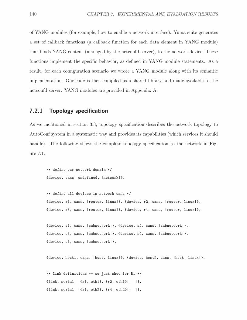
140 CHAPTER 7. EXPERIMENTAL AND EVALUATION RESULTS
of YANG modules (for example, how to enable a network interface). Yuma suite generates
a set of callback functions (a callback function for each data element in YANG module)
that binds YANG content (managed by the netconfd server), to the network device. These
functions implement the specific behavior, as defined in YANG module statements. As a
result, for each configuration scenario we wrote a YANG module along with its semantic
implementation. Our code is then compiled as a shared library and made available to the
netconfd server. YANG modules are provided in Appendix A.
7.2.1 Topology specification
As we mentioned in section 3.3, topology specification describes the network topology to
AutoConf system in a systematic way and provides its capabilities (which services it should
handle). The following shows the complete topology specification to the network in Fig-
ure 7.1.
/* define our network domain */
{device, cans, undefined, [network]},
/* define all devices in network cans */
{device, r1, cans, [router, linux]}, {device, r2, cans, [router, linux]},
{device, r3, cans, [router, linux]}, {device, r4, cans, [router, linux]},
{device, s1, cans, [subnetwork]}, {device, s2, cans, [subnetwork]},
{device, s3, cans, [subnetwork]}, {device, s4, cans, [subnetwork]},
{device, s5, cans, [subnetwork]},
{device, host1, cans, [host, linux]}, {device, host2, cans, [host, linux]},
/* link definitions -- we just show for R1 */
{link, serial, [{r1, eth1}, {r2, eth1}], []},
{link, serial, [{r1, eth2}, {r4, eth2}], []},
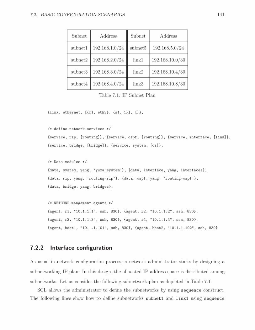
7.2. BASIC CONFIGURATION SCENARIOS 141
Subnet Address Subnet Address
subnet1 192.168.1.0/24 subnet5 192.168.5.0/24
subnet2 192.168.2.0/24 link1 192.168.10.0/30
subnet3 192.168.3.0/24 link2 192.168.10.4/30
subnet4 192.168.4.0/24 link3 192.168.10.8/30
Table 7.1: IP Subnet Plan
{link, ethernet, [{r1, eth3}, {s1, 1}], []},
/* define network services */
{service, rip, [routing]}, {service, ospf, [routing]}, {service, interface, [link]},
{service, bridge, [bridge]}, {service, system, [os]},
/* Data modules */
{data, system, yang, ’yuma-system’}, {data, interface, yang, interfaces},
{data, rip, yang, ’routing-rip’}, {data, ospf, yang, ’routing-ospf’},
{data, bridge, yang, bridges},
/* NETCONF mangement agents */
{agent, r1, "10.1.1.1", ssh, 830}, {agent, r2, "10.1.1.2", ssh, 830},
{agent, r3, "10.1.1.3", ssh, 830}, {agent, r4, "10.1.1.4", ssh, 830},
{agent, host1, "10.1.1.101", ssh, 830}, {agent, host2, "10.1.1.102", ssh, 830}
7.2.2 Interface configuration
As usual in network configuration process, a network administrator starts by designing a
subnetworking IP plan. In this design, the allocated IP address space is distributed among
subnetworks. Let us consider the following subnetwork plan as depicted in Table 7.1.
SCL allows the administrator to define the subnetworks by using sequence construct.
The following lines show how to define subnetworks subnet1 and link1 using sequence

142 CHAPTER 7. EXPERIMENTAL AND EVALUATION RESULTS
construct:
sequence subnet1:ip {192.168.1.0, 24}
sequence link1:ip {192.168.10.0, 30}
To express the interface configuration semantically, we define a new CSM concept called
ifconfig. The schema of this concept is:
schema ifconfig {device, interface, ip, mask}
After that we define an ifconfig semantic view for each interface using the sequence gen-
erator defined previously. For example, to define ifconfig for device R1 semantically:
{ifconfig, r1, eth3, seq:next(subnet1), seq:prefix(subnet1)}
{ifconfig, r1, eth1, seq:next(link1), seq:prefix(link1)}
{ifconfig, r1, eth2, seq:next(link3), seq:prefix(link3)}
The function seq:next() automatically generates a new IP address within the subnetwork
that is specified as argument. The function seq:prefix() returns the network prefix value.
After defining the configuration of all network interfaces, AutoConf takes the specification
and generates an actual IP address plan as shown in Figure 7.2.
Figure 7.2: Interface configuration as generated by AutoConf Executer
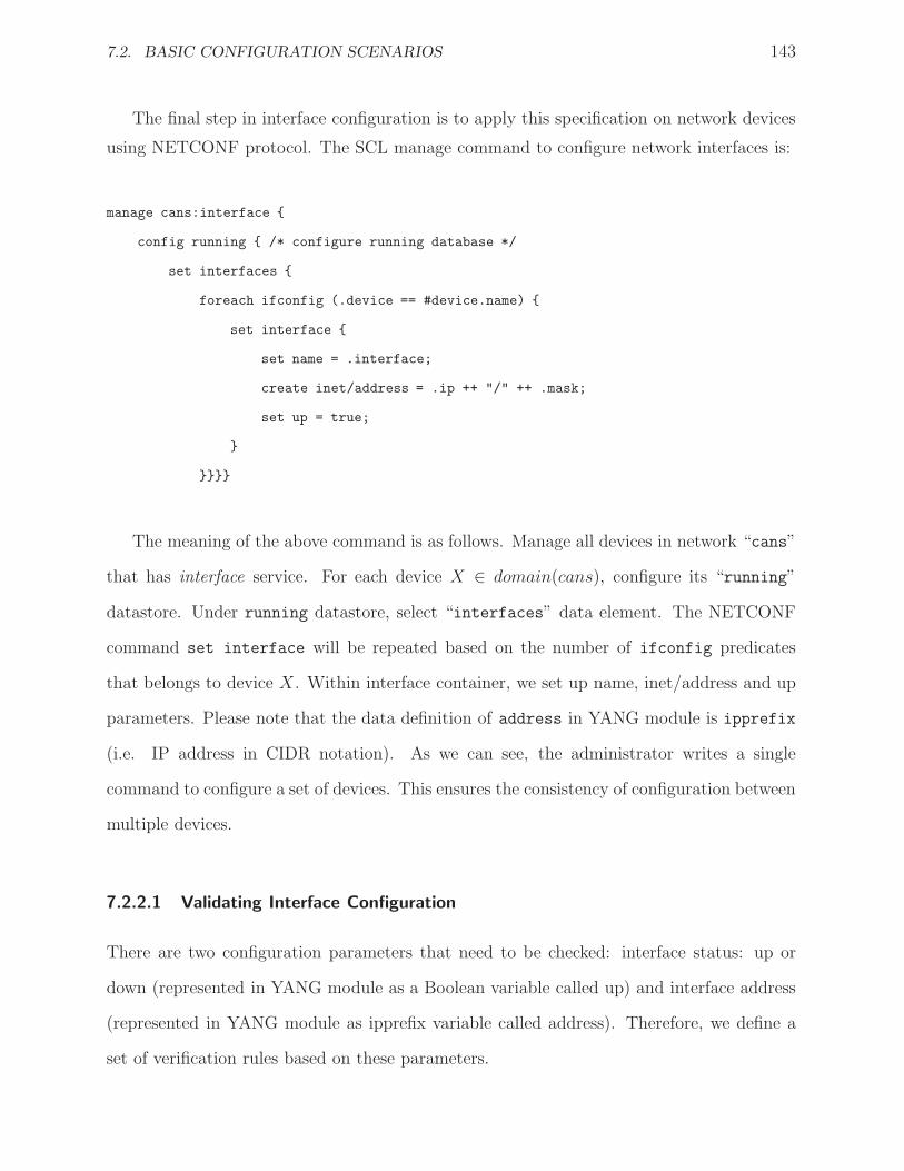
7.2. BASIC CONFIGURATION SCENARIOS 143
The final step in interface configuration is to apply this specification on network devices
using NETCONF protocol. The SCL manage command to configure network interfaces is:
manage cans:interface {
config running { /* configure running database */
set interfaces {
foreach ifconfig (.device == #device.name) {
set interface {
set name = .interface;
create inet/address = .ip ++ "/" ++ .mask;
set up = true;
}
}}}}
The meaning of the above command is as follows. Manage all devices in network “cans”
that has interface service. For each device X ∈ domain(cans), configure its “running”
datastore. Under running datastore, select “interfaces” data element. The NETCONF
command set interface will be repeated based on the number of ifconfig predicates
that belongs to device X . Within interface container, we set up name, inet/address and up
parameters. Please note that the data definition of address in YANG module is ipprefix
(i.e. IP address in CIDR notation). As we can see, the administrator writes a single
command to configure a set of devices. This ensures the consistency of configuration between
multiple devices.
7.2.2.1 Validating Interface Configuration
There are two configuration parameters that need to be checked: interface status: up or
down (represented in YANG module as a Boolean variable called up) and interface address
(represented in YANG module as ipprefix variable called address). Therefore, we define a
set of verification rules based on these parameters.
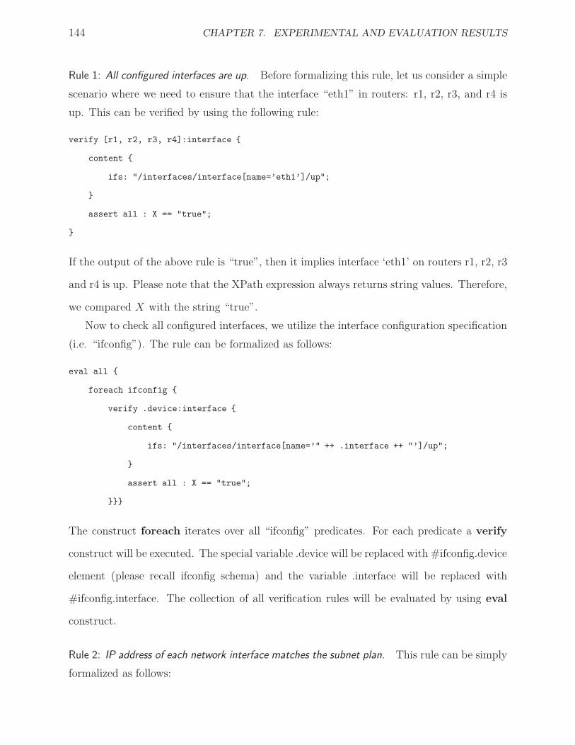
144 CHAPTER 7. EXPERIMENTAL AND EVALUATION RESULTS
Rule 1: All configured interfaces are up. Before formalizing this rule, let us consider a simple
scenario where we need to ensure that the interface “eth1” in routers: r1, r2, r3, and r4 is
up. This can be verified by using the following rule:
verify [r1, r2, r3, r4]:interface {
content {
ifs: "/interfaces/interface[name=’eth1’]/up";
}
assert all : X == "true";
}
If the output of the above rule is “true”, then it implies interface ‘eth1’ on routers r1, r2, r3
and r4 is up. Please note that the XPath expression always returns string values. Therefore,
we compared X with the string “true”.
Now to check all configured interfaces, we utilize the interface configuration specification
(i.e. “ifconfig”). The rule can be formalized as follows:
eval all {
foreach ifconfig {
verify .device:interface {
content {
ifs: "/interfaces/interface[name=’" ++ .interface ++ "’]/up";
}
assert all : X == "true";
}}}
The construct foreach iterates over all “ifconfig” predicates. For each predicate a verify
construct will be executed. The special variable .device will be replaced with #ifconfig.device
element (please recall ifconfig schema) and the variable .interface will be replaced with
#ifconfig.interface. The collection of all verification rules will be evaluated by using eval
construct.
Rule 2: IP address of each network interface matches the subnet plan. This rule can be simply
formalized as follows:
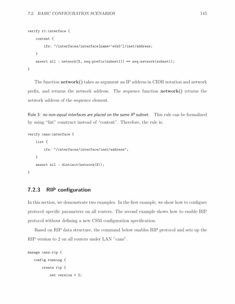
7.2. BASIC CONFIGURATION SCENARIOS 145
verify r1:interface {
content {
ifs: "/interfaces/interface[name=’eth3’]/inet/address;
}
assert all : network(X, seq:prefix(subnet1)) == seq:network(subnet1);
}
The function network() takes as argument an IP address in CIDR notation and network
prefix, and returns the network address. The sequence function network() returns the
network address of the sequence element.
Rule 3: no non-equal interfaces are placed on the same IP subnet. This rule can be formalized
by using “list” construct instead of “content”. Therefore, the rule is:
verify cans:interface {
list {
ifs: "/interfaces/interface/inet/address";
}
assert all : distinct(network(X));
}
7.2.3 RIP configuration
In this section, we demonstrate two examples. In the first example, we show how to configure
protocol–specific parameters on all routers. The second example shows how to enable RIP
protocol without defining a new CSM configuration specification.
Based on RIP data structure, the command below enables RIP protocol and sets up the
RIP version to 2 on all routers under LAN ”cans”.
manage cans:rip {
config running {
create rip {
set version = 2;
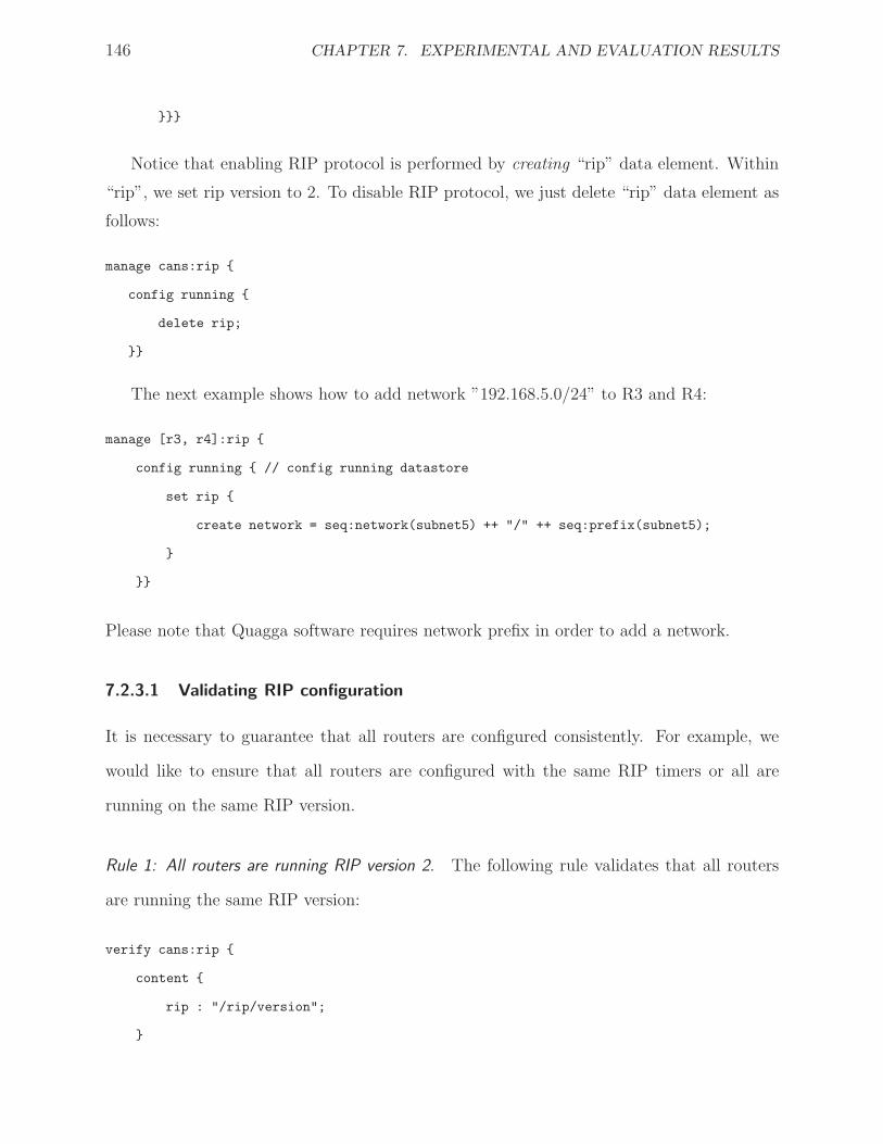
146 CHAPTER 7. EXPERIMENTAL AND EVALUATION RESULTS
}}}
Notice that enabling RIP protocol is performed by creating “rip” data element. Within
“rip”, we set rip version to 2. To disable RIP protocol, we just delete “rip” data element as
follows:
manage cans:rip {
config running {
delete rip;
}}
The next example shows how to add network ”192.168.5.0/24” to R3 and R4:
manage [r3, r4]:rip {
config running { // config running datastore
set rip {
create network = seq:network(subnet5) ++ "/" ++ seq:prefix(subnet5);
}
}}
Please note that Quagga software requires network prefix in order to add a network.
7.2.3.1 Validating RIP configuration
It is necessary to guarantee that all routers are configured consistently. For example, we
would like to ensure that all routers are configured with the same RIP timers or all are
running on the same RIP version.
Rule 1: All routers are running RIP version 2. The following rule validates that all routers
are running the same RIP version:
verify cans:rip {
content {
rip : "/rip/version";
}
7.2. BASIC CONFIGURATION SCENARIOS 147
assert all : int(X) == 2;
}
The function int() coverts the string X to an integer value. Of course, we can write “as-
sert” expression in the same way as we did in interface validation, we just like to demonstrate
the richness of SCL language.
Rule 2: Each router must advertise at least 2 networks. This rule can be formalized by
counting the number network element under rip container:
verify cans:rip {
list {
rip : "/rip/network";
}
assert all : count(X) >= 2;
}
Rule 3: All routers are configured with the same RIP update timer. This rule can be achieved
by collecting update timer from all routers, and then we check for similarity by using
similar() function. The following rule illustrates the process:
verify cans:rip {
list {
rip : "/rip/timers/update";
}
assert all : similar(X);
}
7.2.4 OSPF configuration
In this scenario, we show only without validation the configuration of OSPF protocol using
user–defined CSM concept. The purpose of this concept is to inter–relate between link
attributes since OSPF is a link–state protocol.
148 CHAPTER 7. EXPERIMENTAL AND EVALUATION RESULTS
In this study, we consider the following attributes of a link state: network address, net-
work prefix, area number, and directly connected routers (we ignore other attributes such as
link cost). Consequently, we define a new schema called ospflink that composes of address
(network address), mask (network prefix), area, devices (directly connected devices). The
following shows the schema definition in SCL along with high–level configuration specifica-
tions.
/* ospflink concept */
schema ospflink {address, mask, area, devices}
/* high-level configuration */
insert {
{ospflink, seq:network(subnet1), seq:prefix(subnet1), 0, [r1]},
{ospflink, seq:network(subnet2), seq:prefix(subnet2), 0, [r1]},
{ospflink, seq:network(link1), seq:prefix(link1), 0, [r1, r2]},
{ospflink, seq:network(link2), seq:prefix(link2), 0, [r2, r3]},
{ospflink, seq:network(link3), seq:prefix(link3), 5, [r1, r4]},
{ospflink, seq:network(subnet3), seq:prefix(subnet3), 5, [r3]},
{ospflink, seq:network(subnet4), seq:prefix(subnet4), 5, [r4]},
{ospflink, seq:network(subnet5), seq:prefix(subnet5), 5, [r3, r4]}
}
As noticed, the manager decided to divide the network into two areas: 0 and 5 as
shown in Figure 7.3. Expressing network configuration in high–level abstraction simplifies
configuration process and reduces misconfiguration errors.
Afterwards, the manager can write an SCL command to produce consistent multi-device
configuration:
manage cans:ospf { // manage all devices support OSPF in cans
config running {
foreach ospflink (#device.name in .devices) {
create ospf/network {
set prefix = .address ++ "/" ++ .mask;
set area = .area;
}

7.2. BASIC CONFIGURATION SCENARIOS 149
Subnet2
R2
R1Subnet1
R3
R4 Subnet4
Subnet5
Subnet3
eth3
Link3
Link2
area 0
area 5
Figure 7.3: OSPF links setup
}}}
Notice that foreach statement iterates over all predicates of type ospflink that satisfy
the condition between parenthesis, and executes the inner statement. In large-scale networks,
we can partition the devices into a set of sub-domains. Then each remote AutoConf can
query the distributed database to produce the configuration messages that are related to its
sub-domain.
7.2.5 MPLS VPN Configuration
This study demonstrates the scenario of activating MPLS Layer 3 VPN in service provider
networks for customers. The feature of MPLS VPN is that it allows several sites to intercon-
nect transparently through service provider’s network. Within a VPN, each site can send
IP packets to any other site in the same VPN.
In this scenario, we are going to use the network topology depicted in Figure 7.4 where
routers r4 and r5 are Customer Edge (CE) routers, and routers r2 and r3 are Provider
Edge (PE) routers. Before proceeding, we assume that OSPF protocol and MPLS have
been already configured in the ISP network.
Configuring MPLS VPN requires three steps. The first step is the configuration of virtual
routing and forwarding (VRF) table as well as a set of interfaces that use this VRF entry at

150 CHAPTER 7. EXPERIMENTAL AND EVALUATION RESULTS
Network 192.168.10.0 Network 192.168.20.0
192.168.10.1
10.1.100.18
10.1.100.17
192.168.20.1
10.1.100.27
10.1.100.26
10.1.100.2
10.1.100.9
10.1.100.10
10.1.100.3
R5R4
R2
R1
R3
Figure 7.4: Customer wants to link its two Sites (Site1 and Site2)
the PE routers. The second step is the configuration of PE routers to use Multiprotocol BGP
(MP-BGP) to distribute VPN routing information using MP-BGP extended community.
The third step is the configuration required to implement PE-CE routing sessions which is
depending on the PE-CE routing protocol (e.g. static, RIP, OSPF, etc).
The service provider’s IT team initially designs the set of concepts that describe the
MPLS-VPN service. Let us assume that the description has the following concepts: vpnform,
vpnspec, vpn if. The concept vpnform stores the details of the agreement between the
service provider and the customer. The concept vpnspec describes the configuration speci-
fication to provision a new VPN. The concept vpn if describes which interfaces are facing
customer CE routers. In addition, a domain expert in MPLS VPN configuration is respon-
sible of writing the SCL code to construct the appropriate NETCONF messages based on
the concepts defined above.
When a customer requests a VPN service, he/she fills an appropriate provisioning form.
The form will be forwarded to IT department to initiate the service deployment. A network
operator uses the submitted form and inserts new predicates to the system. The following
script shows the high-level specification of MPLS VPN provisioning request:
insert {
/* custID 100 with bandwidth of 512 */
7.2. BASIC CONFIGURATION SCENARIOS 151
{vpnform,"XYZ company",100,"192.168.0.0",512},
/* vpn name is red with RD 100:1 */
{vpnspec, 100, "red", "100:1", [r3, r4]},
/* specifications for interfaces */
{vpn_if, "red", r3, "fa0/1", "192.168.1.1", 24},
{vpn_if, "red", r4, "fa0/1", "192.168.2.1", 24}
}
Once the above specification has been inserted, the operator only needs to run the SCL
code to generate the NETCONF messages that will be sent to NETCONF servers. The
configuration actually requires several data modules such as VPN MPLS data module, MP-
BGP data module and routing protocol modules. Due to lack of space, we only consider
the configuration of VPN MPLS data module, even without listing the detail of the data
definition.
foreach vpnform (.custid = CUSID) {
foreach vpnspec (.id = #vpnform.custid) {
manage vpnspec.pe:mplsl3vpn {
config running {
set vrf {
set name = #vpnspec.name;
set rd = #vpnspec.rd;
set ’vrf-routing’ {
set policy = "import";
set policy = "export";
}
}
foreach vpn_if (.name = #vpnspec.name and
.router = #device.name) {
create interface {
set name = #vpn_if.interface;
set address = #vpn_if.address;
152 CHAPTER 7. EXPERIMENTAL AND EVALUATION RESULTS
set mask = #vpn_if.mask;
set ’vrf-forwarding’ = #vpn_if.name;
}
}
}
}}}
When the above code is executed, the management system will prompt the user to enter
the customer ID. Thus, the complexity of provisioning a new service has been reduced
by translating the high-level requirement documented in the customer’s form to a set of
predicates.
As indicated above, the main merit of our framework is that it allows different users to
build up service configuration. A network manager, for example, is responsible to define the
concepts needed to specify the configuration. A domain expert is responsible to codify the
specification using SCL language. A network operator uses the defined concepts to create a
set of specifications (based on the guidance of the manager) and executes the appropriate
SCL modules.
7.2.6 Automating interface configuration
We start demonstrating the automation feature in AutoConf management system. First, we
present the interface requirements to automate them. The policy rule specification can be
expressed as follows:
For any device X in CANS, if X:interface:Y is not enabled then call ifconfig(X, Y)
The above policy rule can be translated to generate 14 requirements based on our topology
specification:
{101, host1, interface, eth1, 1, [ifconfig(host1, eth1)]}
{102, host2, interface, eth1, 1, [ifconfig(host2, eth1)]}
{103, r1, interface, eth1, 1, [ifconfig(r1, eth1)]}
.
7.2. BASIC CONFIGURATION SCENARIOS 153
.
{114, r4, interface, eth3, 1, [ifconfig(r4, eth3)]}
When an interface or a link is down, the monitor system should report this incident
to AutoConf using NETCONF notification or SNMP protocol. We manually inserted this
notification to AutoConf system. When AutoConf receives that an interface is down, it
will perform the following actions: (1) updating the system state (2) triggering (by policy
engine) “ifconfig” action to configure the interface at each management cycle, and (3)
updating the new system state when “ifconfig” returns successfully. Note that the Q value
of “ifconfig” will not be incurred when “ifconfig” returns unsuccessfully.
7.2.7 Automating Filtering policy
Now we consider the problem that has been raised in [34]. In this scenario we are going
to run a simulation to examine the behavior of AutoConf to resolve the conflict. The
simulation considers the network topology in Figure 7.1 without link1. The manager defines
the following requirement: Any host in Subnet4 should NOT communicate with any server
in Subnet2. This requirement can be formalized as
{201, network, path, check1, 1, [insert_filter("192.168.4.0/24", deny, R2),
insert_filter("192.168.4.0/24", deny, R3)]}
where network:reach:check1 is the verification rule:
policy [subnet4, subnet1]:path {
assert (action=0)
}
We expect that this rule will be executed by the monitor system to verify the network
behavior. When this rule is violated, it will emit the following network state {network,
path, check1, 0}.
Based on our requirement, when AutoConf receives {network, path, check1, 0}, it has two
choices to fix the conflict: running insert filter at router R2 or running insert filter
154 CHAPTER 7. EXPERIMENTAL AND EVALUATION RESULTS
at router R3. We setup our experiment such that AutoConf selection is biased in the favor
of inserting filtering policy at router R3.
In our first run, we injected AutoConf {network, path, check1, 0}. AutoConf invoked
first action from the first management cycle. In our experiment the management cycle was
15 seconds. Thus, the average repair time is 7.5 seconds.
We modified the two actions such that the first action modifies the network state by
injecting {network, path, check1, 0}, while the second action modifies the network state by
injecting {network, path, check1, 1}. This modification is to simulate the case when we add
link1 to the network topology. Inserting filter policy at router R3 will not fix the problem.
We observed the following behavior: In the first and the second management cycle,
AutoConf has selected the first action. Then it has adjusted its decision in the favor of the
second action in the third management cycle. This implies that the correction has been
fixed in 37.5 seconds in average.
Now, we injected {network, path, check1, 0} again. AutoConf fixed the conflict imme-
diately in the next management cycle. The average repair time is 7.5 seconds.
We kept injecting {network, path, check1, 0} at random times. At the 7th injection, the
management system has selected the first action, then it has selected the second action. At
7th injection, the average repair time was 22.5.
7.3 Evaluating Verification System using Simulation
In order to thoroughly test our verification framework, we must test it against large–scale
networks with varying parameters and sizes. Using only real configuration will limit the
number of evaluation scenarios. As such we have developed a tool called netgen to generate
randomly networks along with valid forwarding control rules. We also modify AutoConf
system to accept the tool results. Forwarding access rules are generated as plain text instead
of XML files.

7.3. EVALUATING VERIFICATION SYSTEM USING SIMULATION 155
We run our evaluation on a computer with Intel Core 2 Duo CPU 2.13GHz and 4GB of
RAM. We generated 15 different scenarios with different network sizes. Five scenarios have
been configured to generate huge set of complex firewall policies. The remaining scenarios
are used to evaluate AutoConf’s capability to handle FCL’s. The average number of nodes is
600 with 10,000 links. The average total number of FCL rules is 100,000 rules per network.
7.3.1 Topology and FCL Generator
Netgen generates randomly a network topology that consists of three types of nodes: router
node, firewall node, and subnet node. Router and subnet nodes are initially placed in a
rectangular plane of size H×W where H and W are matrix height and width, respectively.
Matrix height determines the number of levels (hierarchical levels) where nodes in level 1
are always core routers and nodes in level H are always subnet nodes. The distribution
of subnet nodes and router nodes in the remaining levels follow a power law probability
distribution such that the number of subnets decreases as the level number reaches 1. After
placing subnet and router nodes, we interconnect two nodes using the following model:
• The number of links between two levels is controlled by a parameter called branching
factor and the number of routers in the upper level.
• Each node at level i is connected to at least one router node at level i − 1. The
selection of router node follows a uniform distribution. If the branching factor for that
router has been reached, the next router (to the right) is selected. Please note if the
branching factor for all routers at level i−1 has been reached, the first selected router
will be used.
• There is no link between a subnet node at level i and any node at level i+ 1.
• There is no link between two nodes at the same level, except core routers at level 1.
There is a link between two adjacent core routers.

156 CHAPTER 7. EXPERIMENTAL AND EVALUATION RESULTS
The above model guarantees that we have one connected network topology and the
maximum path length is 2× (H − 1) +W .
The next step is to place firewall nodes on links. The number of firewalls is determined by
a given percentage. The distribution of firewalls in the graph follows Exponential distribution
such that the number of firewall increases as the level number increases.
The routing distribution follows a modified version of RIP protocol. Each lower level
router advertises its routing tables to the upper level routers. There is no advertisement
from upper level routers to lower level routers. All routers, except the left-most core router,
have a default gateway. Firewall rules are generated randomly. However, the address space
in each firewall is divided into two sets: internal addresses and external addresses. Internal
addresses are the set of all subnet addresses from subnet nodes that are directly or indirectly
connected to the firewall node. The remain address space is called external space. Therefore,
if a firewall rule consists of source IP address and destination IP address, then one address
must be internal and the other address must be external.
7.3.2 Evaluating BDD Construction
We first show the improved performance of using Equation 4.7 rather than Equation 4.4.
Firewall policy is considered the most complex and costly in BDD construction than other
policies since it involves all packet header information. Therefore, it is very crucial to
evaluate our new algorithm rigorously in terms of memory and time complexities. We
configured policy generator to generate random firewall rules as shown in List 8.
Figure 7.5(a) depicts the behavior of old Equation 4.4 and new Equation 4.7 when
deny icmp 94.89.242.151 255.255.240.0 18.2.113.185 255.255.255.240
accept udp 18.2.48.196 255.255.255.248 any 159.89.0.0 255.255.0.0 796-1340
accept tcp 64.95.143.128 255.255.252.0 22 18.2.214.214 255.255.128.0 any
accept udp 12.1.24.0 255.255.224.0 21 18.2.130.128 255.255.255.128 1233-6502
deny any 109.102.96.218 255.255.255.254 any 18.2.250.208 255.255.255.240 21
List 8: Sample of Firewall rules generated by NetGen

7.3. EVALUATING VERIFICATION SYSTEM USING SIMULATION 157
0
200
400
600
800
1000
1200
1400
1600
1800
2000
0 1000 2000 3000 4000 5000 6000
Num
ber
of B
DD
nod
es (
in T
hous
ands
)
Number of Rules
New FormulaOld Formula
(a) GC is invoked by Buddy
0
50
100
150
200
250
0 1000 2000 3000 4000 5000 6000
Num
ber
of B
DD
nod
es (
in T
hous
ands
)
Number of Rules
New FormulaOld Formula
(b) GC is invoked explicitly after each rule
Figure 7.5: Comparing between Equation 4.7 and Equation 4.4 in terms of memory com-plexity
Work # of rules Time (in secs) Our Time (in secs)FIREMAN [101] 800 2 0.18ConfigChecker [1] 200,000 1100 116
Quarnet [55] 56,189 126 18
Table 7.2: Time Performance as reported in previous work
constructing a Boolean expression for a firewall policy. We set the maximum number of
BDD nodes in Buddy’s cache memory to 2 millions nodes. These nodes are used by Buddy
when performing BDD operations. It is clearly evident that the old equation (shown as a
thick line) is more expensive than the new equation (shown as thin line) because it consumes
the cache memory very quickly. Notice that Buddy automatically invokes garbage collection
engine to free the cache memory. Figure 7.5(b) shows the space complexity of each equation
when the number of rules is less than six thousands. The space complexity of the new
equation is almost half of the space complexity of the old equation.
Table 7.2 shows the performance of our new Equation compared to previous work in
literature. FIREMAN took less than 3 seconds to construct an ACL with 800 rules as
reported in [101]. Quarnet took 2.1 minutes to construct approximately 56 thousands of
stateful firewall rules. ConfigChecker constructed 200 thousands rules in approximately
18.3 minutes.
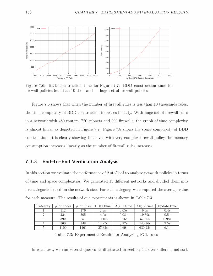
158 CHAPTER 7. EXPERIMENTAL AND EVALUATION RESULTS
0
500
1000
1500
2000
2500
3000
3500
1000 2000 3000 4000 5000 6000 7000 8000 9000 10000
Tim
e in
(m
illis
econ
ds)
Number of FW Rules
Time
Figure 7.6: BDD construction time forfirewall policies less than 10 thousands
0
200
400
600
800
1000
1200
1400
1600
0 200 400 600 800 1000 1200
Tim
e in
(se
cs)
Number of FW Rules (in thousands)
Time
Figure 7.7: BDD construction time forhuge set of firewall policies
Figure 7.6 shows that when the number of firewall rules is less than 10 thousands rules,
the time complexity of BDD construction increases linearly. With huge set of firewall rules
in a network with 480 routers, 720 subnets and 200 firewalls, the graph of time complexity
is almost linear as depicted in Figure 7.7. Figure 7.8 shows the space complexity of BDD
construction. It is clearly showing that even with very complex firewall policy the memory
consumption increases linearly as the number of firewall rules increases.
7.3.3 End–to–End Verification Analysis
In this section we evaluate the performance of AutoConf to analyze network policies in terms
of time and space complexities. We generated 15 different networks and divided them into
five categories based on the network size. For each category, we computed the average value
for each measure. The results of our experiments is shown in Table 7.3.
Category # of nodes # of links BDD time Alg. 1 time Alg. 2 time Update time1 112 179 2.3s 0.05s 9.6s 0.4s2 224 305 4.6s 0.08s 19.39s 0.5s3 392 551 10.16s 0.16s 57.06s 0.98s4 560 748 14.27s 0.27s 140.76s 2.5s5 1100 1401 27.32s 0.69s 630.22s 6.1s
Table 7.3: Experimental Results for Analyzing FCL rules
In each test, we run several queries as illustrated in section 4.4 over different network
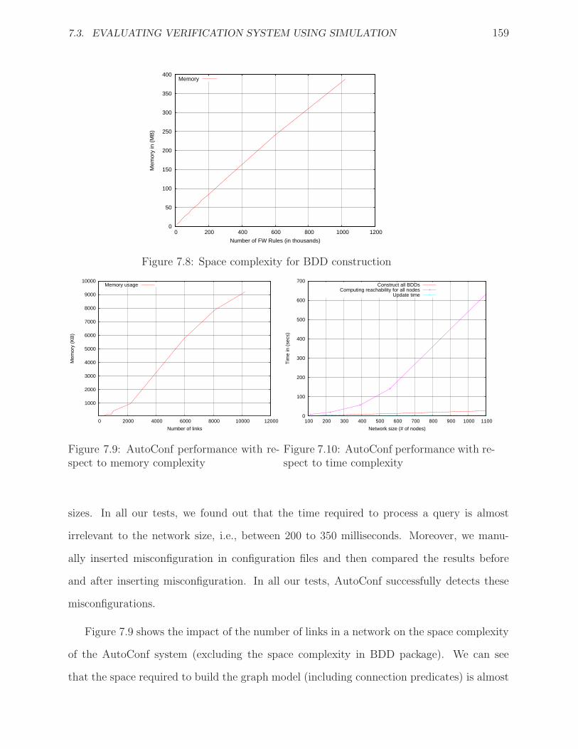
7.3. EVALUATING VERIFICATION SYSTEM USING SIMULATION 159
0
50
100
150
200
250
300
350
400
0 200 400 600 800 1000 1200
Mem
ory
in (
MB
)
Number of FW Rules (in thousands)
Memory
Figure 7.8: Space complexity for BDD construction
1000
2000
3000
4000
5000
6000
7000
8000
9000
10000
0 2000 4000 6000 8000 10000 12000
Mem
ory
(KB
)
Number of links
Memory usage
Figure 7.9: AutoConf performance with re-spect to memory complexity
0
100
200
300
400
500
600
700
100 200 300 400 500 600 700 800 900 1000 1100
Tim
e in
(se
cs)
Network size (# of nodes)
Construct all BDDsComputing reachability for all nodes
Update time
Figure 7.10: AutoConf performance with re-spect to time complexity
sizes. In all our tests, we found out that the time required to process a query is almost
irrelevant to the network size, i.e., between 200 to 350 milliseconds. Moreover, we manu-
ally inserted misconfiguration in configuration files and then compared the results before
and after inserting misconfiguration. In all our tests, AutoConf successfully detects these
misconfigurations.
Figure 7.9 shows the impact of the number of links in a network on the space complexity
of the AutoConf system (excluding the space complexity in BDD package). We can see
that the space required to build the graph model (including connection predicates) is almost
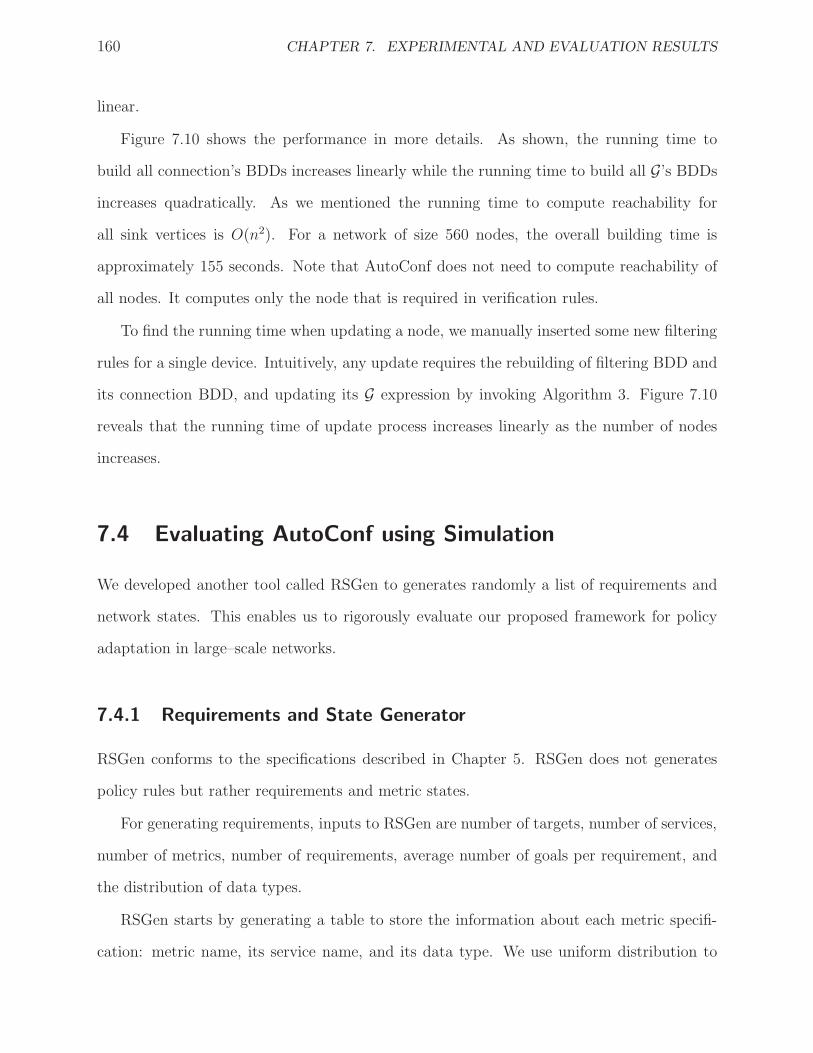
160 CHAPTER 7. EXPERIMENTAL AND EVALUATION RESULTS
linear.
Figure 7.10 shows the performance in more details. As shown, the running time to
build all connection’s BDDs increases linearly while the running time to build all G’s BDDs
increases quadratically. As we mentioned the running time to compute reachability for
all sink vertices is O(n2). For a network of size 560 nodes, the overall building time is
approximately 155 seconds. Note that AutoConf does not need to compute reachability of
all nodes. It computes only the node that is required in verification rules.
To find the running time when updating a node, we manually inserted some new filtering
rules for a single device. Intuitively, any update requires the rebuilding of filtering BDD and
its connection BDD, and updating its G expression by invoking Algorithm 3. Figure 7.10
reveals that the running time of update process increases linearly as the number of nodes
increases.
7.4 Evaluating AutoConf using Simulation
We developed another tool called RSGen to generates randomly a list of requirements and
network states. This enables us to rigorously evaluate our proposed framework for policy
adaptation in large–scale networks.
7.4.1 Requirements and State Generator
RSGen conforms to the specifications described in Chapter 5. RSGen does not generates
policy rules but rather requirements and metric states.
For generating requirements, inputs to RSGen are number of targets, number of services,
number of metrics, number of requirements, average number of goals per requirement, and
the distribution of data types.
RSGen starts by generating a table to store the information about each metric specifi-
cation: metric name, its service name, and its data type. We use uniform distribution to
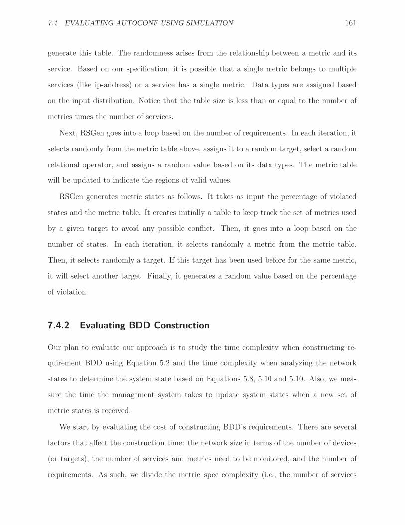
7.4. EVALUATING AUTOCONF USING SIMULATION 161
generate this table. The randomness arises from the relationship between a metric and its
service. Based on our specification, it is possible that a single metric belongs to multiple
services (like ip-address) or a service has a single metric. Data types are assigned based
on the input distribution. Notice that the table size is less than or equal to the number of
metrics times the number of services.
Next, RSGen goes into a loop based on the number of requirements. In each iteration, it
selects randomly from the metric table above, assigns it to a random target, select a random
relational operator, and assigns a random value based on its data types. The metric table
will be updated to indicate the regions of valid values.
RSGen generates metric states as follows. It takes as input the percentage of violated
states and the metric table. It creates initially a table to keep track the set of metrics used
by a given target to avoid any possible conflict. Then, it goes into a loop based on the
number of states. In each iteration, it selects randomly a metric from the metric table.
Then, it selects randomly a target. If this target has been used before for the same metric,
it will select another target. Finally, it generates a random value based on the percentage
of violation.
7.4.2 Evaluating BDD Construction
Our plan to evaluate our approach is to study the time complexity when constructing re-
quirement BDD using Equation 5.2 and the time complexity when analyzing the network
states to determine the system state based on Equations 5.8, 5.10 and 5.10. Also, we mea-
sure the time the management system takes to update system states when a new set of
metric states is received.
We start by evaluating the cost of constructing BDD’s requirements. There are several
factors that affect the construction time: the network size in terms of the number of devices
(or targets), the number of services and metrics need to be monitored, and the number of
requirements. As such, we divide the metric–spec complexity (i.e., the number of services
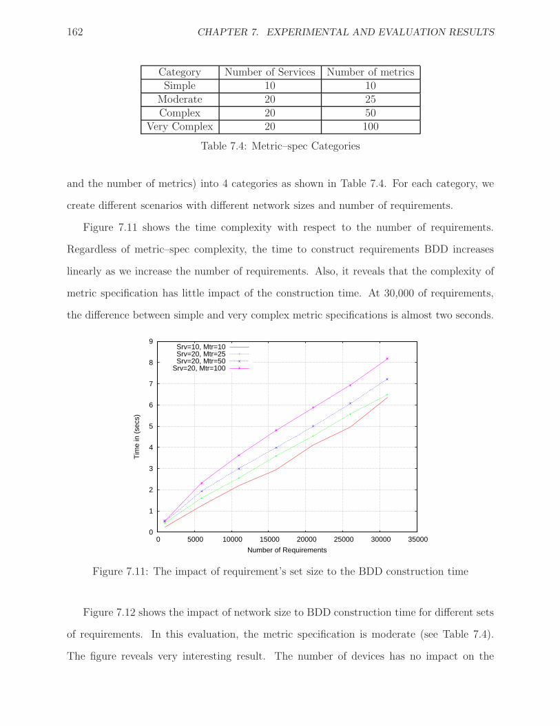
162 CHAPTER 7. EXPERIMENTAL AND EVALUATION RESULTS
Category Number of Services Number of metricsSimple 10 10
Moderate 20 25Complex 20 50
Very Complex 20 100
Table 7.4: Metric–spec Categories
and the number of metrics) into 4 categories as shown in Table 7.4. For each category, we
create different scenarios with different network sizes and number of requirements.
Figure 7.11 shows the time complexity with respect to the number of requirements.
Regardless of metric–spec complexity, the time to construct requirements BDD increases
linearly as we increase the number of requirements. Also, it reveals that the complexity of
metric specification has little impact of the construction time. At 30,000 of requirements,
the difference between simple and very complex metric specifications is almost two seconds.
0
1
2
3
4
5
6
7
8
9
0 5000 10000 15000 20000 25000 30000 35000
Tim
e in
(se
cs)
Number of Requirements
Srv=10, Mtr=10Srv=20, Mtr=25Srv=20, Mtr=50
Srv=20, Mtr=100
Figure 7.11: The impact of requirement’s set size to the BDD construction time
Figure 7.12 shows the impact of network size to BDD construction time for different sets
of requirements. In this evaluation, the metric specification is moderate (see Table 7.4).
The figure reveals very interesting result. The number of devices has no impact on the
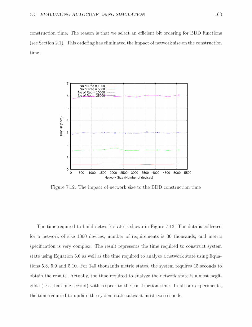
7.4. EVALUATING AUTOCONF USING SIMULATION 163
construction time. The reason is that we select an efficient bit ordering for BDD functions
(see Section 2.1). This ordering has eliminated the impact of network size on the construction
time.
0
1
2
3
4
5
6
7
0 500 1000 1500 2000 2500 3000 3500 4000 4500 5000 5500
Tim
e in
(se
cs)
Network Size (Number of devices)
No of Req = 1000No of Req = 5000
No of Req = 10000No of Req = 25000
Figure 7.12: The impact of network size to the BDD construction time
The time required to build network state is shown in Figure 7.13. The data is collected
for a network of size 1000 devices, number of requirements is 30 thousands, and metric
specification is very complex. The result represents the time required to construct system
state using Equation 5.6 as well as the time required to analyze a network state using Equa-
tions 5.8, 5.9 and 5.10. For 140 thousands metric states, the system requires 15 seconds to
obtain the results. Actually, the time required to analyze the network state is almost negli-
gible (less than one second) with respect to the construction time. In all our experiments,
the time required to update the system state takes at most two seconds.
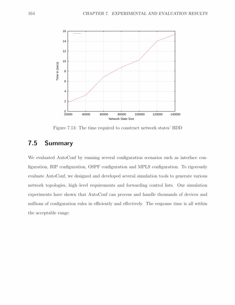
164 CHAPTER 7. EXPERIMENTAL AND EVALUATION RESULTS
0
2
4
6
8
10
12
14
16
20000 40000 60000 80000 100000 120000 140000
Tim
e in
(se
cs)
Network State Size
Figure 7.13: The time required to construct network states’ BDD
7.5 Summary
We evaluated AutoConf by running several configuration scenarios such as interface con-
figuration, RIP configuration, OSPF configuration and MPLS configuration. To rigorously
evaluate AutoConf, we designed and developed several simulation tools to generate various
network topologies, high–level requirements and forwarding control lists. Our simulation
experiments have shown that AutoConf can process and handle thousands of devices and
millions of configuration rules in efficiently and effectively. The response time is all within
the acceptable range.

Chapter 8
Conclusion
Managing large networks is extremely complex and error-prone. Automating network config-
uration is a challenging topic in networking research. Successful network management should
not only ensure the correctness of current service configuration but also should guarantee
service delivery during the life cycle of managed networks. This dissertation is an attempt
to tackle two major problems in network configuration: (1) installation and provisioning of
services in a heterogeneous network, and (2) reconfiguration as to maintain reachability, secu-
rity and performance requirements. We designed a configuration management system called
AutoConf not only to automate service configuration but also to adapt its configuration
to fulfill high–level requirements. AutoConf consists of three main components: Network
Configuration System, Network Verification System and Network Automation System.
We presented in–depth review of the continuous effort of standardized organization to
tackle network management and the latest effort of IETF to improve the network con-
figuration management: NETCONF protocol and YANG data model. While NETCONF
and YANG provide more effective and simpler configuration management to deal with the
proprietary configuration data in heterogeneous networks, there is a limited effort on stan-
dardizing common configuration information as in SNMP MIB definitions. Network Con-
figuration System handles this limitation by taking as input Configuration Semantic Model
165
166 CHAPTER 8. CONCLUSION
describing a network and a set of SCL templates for various service configuration that will
be translated to generate valid NETCONF-based configuration messages. From these speci-
fication, AutoConf generates complete, consistent network configuration on the fly. To truly
evaluate the usefulness of the proposed configuration solution, we run AutoConf with dif-
ferent configuration scenarios. We demonstrated how to use CSM abstraction to design and
plan the network information. We also demonstrated the interface, RIP, OSPF and MPLS
configurations.
General configuration practice is to verify the uploaded configuration and to ensure that
the network is operated as intended. We presented a global network verification system that
ensures not only the consistency of configuration values that span multiple devices but also
the correct behavior for end–to–end reachability and security properties. We introduced a
new formalization for modeling routing tables based on prefix length. We also improved
the formalization of filtering policies as well as NAT policies. To rigorously evaluate the
evaluation system, we designed and developed a topology and configuration generator. We
generated different networks that consist cumulatively thousands to millions forwarding
control rules. Our experimental results show significant improvement over previous work.
Network Automation System adopts policy–based management for automation and adap-
tation. Sometimes the network administrator has multiple choices to handle policy conflicts.
To enable AutoConf to figure out the best choice, we implemented Dyna-Q algorithm, which
is a Q-learning technique that allows the system to learn on–line. We also presented a novel
formalization for modeling configuration and expectation policies in order to have a compact
representation and to enable us to use Dyna-Q with large–sized networks.
8.1 Limitations
The work presented here is designed to reduce configuration complexity. Our key design
philosophy is practicality such that it can immediately be applied to any current network.
8.2. FUTURE WORK 167
However, we still need to overcome the following limitations:
• Not all network devices support NETCONF or YANG architectures. Even though we
can resolve it by deploying proxy NETCONF-enabled servers, developing one proxy
server can be tedious specially in heterogeneous network infrastructure.
• We assume that YANG modules have different module’s prefixes. The purpose of
module prefix is to uniquely identify the configuration data within a single module.
Since there are no common agreement on management information under NETCONF
umbrella, it is possible to have two different modules with the same module prefix. We
can resolve this limitation by augmenting module prefix with its namespace. However,
namespaces are long and difficult to implement.
• Our adaptive technique learns by trials. It must try all alternative in order to find the
best action. Although all alternative actions are based on administration experience,
it is possible that one action can put the network in critical state. In the future,
this action will not be selected again but it must be tried. We can avoid this from
happening by running in a logical network such as ShadowNet [20] to learn the optimal
policy.
8.2 Future work
We summarize here some of future areas suggested by our work.
• We designed our management system to adopt other standard management protocols
by adding Erlang modules during its running time. However, we did not implement
it. Also, it needs to analyze the capabilities of network devices by correlating between
device type with vendor-specific MIBs to build up device database. In NETCONF,
we achieved this by analyzing the advertised capabilities when exchanging HELLO
message.

168 CHAPTER 8. CONCLUSION
• In this dissertation, we analyzed filtering, routing and NAT’ing policies. We are plan-
ning to extend this analysis by accommodating other policies such as IPSec.
• We designed our system using the Q-learning technique due to its computational at-
traction and no assumption is required for model convergence. In literature, there
are some evidence that function approximation provides better average reward after a
long run. The advantage of function approximation is that it does not require memory
to store states. So, it is very suitable for learning the behavior of large–scale net-
works. However, it requires extensive computation and training to optimize function
parameters. We are planning to investigate the applicability of using function approx-
imation in network configuration management and measure its effectiveness compared
to Q-learning technique.
• The management system we design has text-based interface. We are planning to extend
our implementation to support graphical user interface.
Bibliography
[1] E. Al-Shaer, W Marrero, A. El-Atawy, and K. Elbadawi. Network configuration in a box:
towards end-to-end verification of network reachability and security. In Proceedings of 17th
International Conference on Network Protocols (ICNP), pages 123–132. IEEE, October 2009.
[cited at p. 58, 74, 157]
[2] Arbor Networks Inc. Worldwide infrastructure security report, volume vi.
http://www.arbornetworks.com/report, 2010. [cited at p. 3]
[3] Joe Armstrong, Robert Virding, and Mike Williams. Concurrent Programming in Erlang.
Prentice Hall International (UK), 2nd edition, 1996. [cited at p. 125, 127]
[4] D. Durham at el. The COPS (Common Open Policy Service) Protocol. RFC 2748, January
2000. [cited at p. 53]
[5] Avaya Labs. Xml based management interface for snmp enabled devices.
http://www.research.avayalabs.com/user/mazum/Projects/XML. [cited at p. 51]
[6] Ricardo Bagnasco and Joan Serrat. Multi-agent reinforcement learning in network manage-
ment. In Proceedings of the 3rd International Conference on Autonomous Infrastructure,
Management and Security: Scalability of Networks and Services, AIMS ’09, pages 199–202,
Berlin, Heidelberg, 2009. Springer-Verlag. [cited at p. 106]
[7] R.M. Bahati and M.A. Bauer. Towards adaptive policy-based management. In Net-
work Operations and Management Symposium (NOMS), 2010 IEEE, pages 511–518, 2010.
[cited at p. 105, 118, 119]
169

170 BIBLIOGRAPHY
[8] Hitesh Ballani and Paul Francis. Conman: a step towards network manageability. In Pro-
ceedings of the 2007 conference on Applications, technologies, architectures, and protocols
for computer communications, SIGCOMM ’07, pages 205–216, New York, NY, USA, 2007.
ACM. [cited at p. 55]
[9] Franck Barillaud, Luca Deri, and Metin Feridun. Network management using internet tech-
nologies. In 5th IFIP/IEEE International Symposium on Integrated Network Management
(IM’97), pages 61–70, May 1997. [cited at p. 51]
[10] Paul Barry. Programming the network with Perl. John Wiley & Sons Ltd, 2002. [cited at p. 49]
[11] M. Bjorklund. YANG A data modeling language for Network Configuration Protocol (NET-
CONF). RFC 6020, October 2010. [cited at p. 5]
[12] Raymond Blair and Arvind Durai. Tcl scripting for Cisco IOS. Cisco Press, 2010.
[cited at p. 49]
[13] Staffan Blau et al. Axd 301: a new generation atm switching system. Computer Networks,
31(6):559–582, 1999. [cited at p. 125]
[14] Raouf Boutaba and Jin Xiao. Network management: State of the art. In Proceedings of the
IFIP 17th World Computer Congress - TC6 Stream on Communication Systems: The State
of the Art, pages 127–146, 2002. [cited at p. 53]
[15] Caroline Chappell. Creating the programmable network: The business case for netconf/yang
in network devices. Whitepaper on Behalf of Tail-f, October 2013. [cited at p. 5]
[16] Martin Casado, Michael J. Freedman, Justin Pettit, Jianying Luo, Nick McKeown, and Scott
Shenker. Ethane: taking control of the enterprise. In Proceedings of the 2007 conference on
Applications, technologies, architectures, and protocols for computer communications, SIG-
COMM ’07, pages 1–12, New York, NY, USA, 2007. ACM. [cited at p. 55]
[17] J. Case, R. Mundy, D. Partain, and B. Stewart. Introduction and Applicability Statements
for Internet Standard Management Framework. RFC 3410, December 2000. [cited at p. 32]

BIBLIOGRAPHY 171
[18] Xu Chen, Z. Morley Mao, and Jacobus van der Merwe. Towards automated network man-
agement: network operations using dynamic views. In Proceedings of the 2007 SIGCOMM
workshop on Internet network management, INM ’07, pages 242–247, New York, NY, USA,
2007. ACM. [cited at p. 103]
[19] Xu Chen, Z. Morley Mao, and Jacobus Van der Merwe. Pacman: a platform for automated
and controlled network operations and configuration management. In Proceedings of the 5th
international conference on Emerging networking experiments and technologies, CoNEXT
’09, pages 277–288. ACM, 2009. [cited at p. 103, 105]
[20] Xu Chen, Z. Morley Mao, and Jacobus Van Der Merwe. Shadownet: a platform for rapid
and safe network evolution. In Proceedings of the 2009 conference on USENIX Annual
technical conference, USENIX’09, pages 3–3, Berkeley, CA, USA, 2009. USENIX Association.
[cited at p. 167]
[21] Mi-Jung Choi, James W. Hong, and Hong-Taek Ju. Xml-based network management
for ip networks. Electronics and Telecommunications Research Institute (ETRI) Journal,
25(6):445–463, December 2003. [cited at p. 51]
[22] Douglas E. Comer. Automated Network Management Systems: Current and Future Capabil-
ities. Pearson Education, Inc, 1st edition, 2006. [cited at p. 4]
[23] Nicodemos Damianou. A Policy Framework for Management of Distributed Systems. PhD
thesis, Imperial College London, March 2002. [cited at p. 103]
[24] Nicodemos Damianou, Naranker Dulay, Emil Lupu, and Morris Sloman. The ponder pol-
icy specification language. In Proceedings of the International Workshop on Policies for
Distributed Systems and Networks, POLICY ’01, pages 18–38, London, UK, 2001. Springer-
Verlag. [cited at p. 54, 106]
[25] Jianguo Ding. Advances in Network Management. CRC Press, 2010. [cited at p. 36]
[26] William Enck, Patrick McDaniel, Subhabrata Sen, Panagiotis Sebos, Sylke Spoerel, Al-
bert Greenberg, Sanjay Rao, and William Aiello. Configuration management at massive
172 BIBLIOGRAPHY
scale: System design and experience. IEEE Journal on Selected Areas in Communications,
27(3):323–335, April 2009. [cited at p. 49]
[27] R. Enns. NETCONF configuration protocol. RFC 4741, December 2006. [cited at p. 5]
[28] J. Lind-Nielsen et al. Buddy, a binary decision diagram library.
http://buddy.sourceforge.net/, 1992. [cited at p. 14]
[29] Nick Feamster and Hari Balakrishnan. Detecting bgp configuration faults with static anal-
ysis. In Proceedings of the 2nd conference on Symposium on Networked Systems Design &
Implementation - Volume 2, NSDI’05, pages 43–56. USENIX Association, 2005. [cited at p. 57]
[30] Frank Strauss et al. Libsmi. http://www.ibr.cs.tu-bs.de/projects/libsmi. [cited at p. 51]
[31] Scott Lystig Fritchie. A study of erlang ets table implementations and performance. In
Proceedings of the 2003 ACM SIGPLAN workshop on Erlang, ERLANG ’03, pages 43–55,
New York, NY, USA, 2003. ACM. [cited at p. 126]
[32] Patrick Goldsack, Julio Guijarro, Steve Loughran, Alistair Coles, Andrew Farrell, Antonio
Lain, Paul Murray, and Peter Toft. The smartfrog configuration management framework.
ACM SIGOPS Operating Systems Review, 43(1):16–25, 2009. [cited at p. 52]
[33] Mohamed G. Gouda and Alex X. Liu. Structured firewall design. Comput. Netw., 51:1106–
1120, March 2007. [cited at p. 57, 74, 84, 87]
[34] Albert Greenberg, Gisli Hjalmtysson, David A. Maltz, Andy Myers, Jennifer Rexford, Ge-
offrey Xie, Hong Yan, Jibin Zhan, and Hui Zhang. A clean slate 4d approach to network
control and management. SIGCOMM Comput. Commun. Rev., 35(5):41–54, October 2005.
[cited at p. 54, 90, 153]
[35] Natasha Gude, Teemu Koponen, Justin Pettit, Ben Pfaff, Martın Casado, Nick McKeown,
and Scott Shenker. Nox: towards an operating system for networks. SIGCOMM Comput.
Commun. Rev., 38(3):105–110, July 2008. [cited at p. 55]

BIBLIOGRAPHY 173
[36] Hazem Hamed, Ehab Al-Shaer, and Will Marrero. Modeling and verification of ipsec and
vpn security policies. In Proceedings of the 13TH IEEE International Conference on Network
Protocols (ICNP’05), pages 259–278, Washington, DC, USA, 2005. [cited at p. 57, 87]
[37] Heinz-Gerd Hegering, Sebastian Abeck, and Bernhard Neumair. Integrated Management of
Networked Systems: Concepts, Architectures, and Their Operational Application. Morgan
Kaufmann, 1999. [cited at p. 1, 36]
[38] Urs Hoelzle and Luiz Andre Barroso. The Datacenter as a Computer: An Introduction to the
Design of Warehouse-Scale Machines. Morgan and Claypool Publishers, 1st edition, 2009.
[cited at p. 4]
[39] ISO/IEC 10026-1. Information technology - Open Systems Interconnection - Distributed
Transaction Processing - Part 1: OSI TP Model, 1998. [cited at p. 25]
[40] ISO/IEC 10040. Information Processing Systems - Open Systems Interconnection - Systems
Management Overview, 1992. [cited at p. 19]
[41] ISO/IEC 10165-1. Information Processing Systems - Open Systems Interconnection - Struc-
ture of Management Information: Management Information Model, 1993. [cited at p. 20]
[42] ISO/IEC 10731. Information Processing Systems - Open Systems Interconnection - Basic
Reference Model: Conventions for the definition of OSI services, 1994. [cited at p. 24]
[43] ISO/IEC 7498. Information Processing Systems - Open Systems Interconnection - Basic
Reference Model, 1984. [cited at p. 19]
[44] ISO/IEC 7498-4. Information Processing Systems - Open Systems Interconnection - Basic
Reference Model - Part 4: Management Framework, 1989. [cited at p. 1, 19]
[45] ISO/IEC 8571-1. Information technology - Open Systems Interconnection - File Transfer,
Access and Management - Part 1: General Introduction, 1988. [cited at p. 25]
[46] ISO/IEC 8649. Information technology - Open Systems Interconnection - Service Definition
for the Association Control Service Element, 1999. [cited at p. 24]

174 BIBLIOGRAPHY
[47] ISO/IEC 8824-1. Information technology - Open Systems Interconnection - Abstract Syntax
Notation One (ASN.1): Specification of basic notation, 2008. [cited at p. 21]
[48] ITU-T Recommendation M.3010. Telecommunications Management Network, Principles for
a Telecommunications Management Network, 2000. [cited at p. 1, 25]
[49] B. Jennings, S. van der Meer, S. Balasubramaniam, D. Botvich, M.O. Foghlu, W. Donnelly,
and J. Strassner. Towards autonomic management of communications networks. Communi-
cations Magazine, IEEE, 45(10):112 –121, October 2007. [cited at p. 52]
[50] Hong-Taek Ju, Mi-Jung Choi, Sehee Han, Yunjung Oh, Jeong-Hyuk Yoon, Hyojin Lee, and
J.W. Hong. An embedded web server architecture for xml-based network management. In
Network Operations and Management Symposium, 2002. NOMS 2002. 2002 IEEE/IFIP,
pages 5–18, 2002. [cited at p. 51]
[51] Juniper Networks. Junos xml api. http://www.juniper.net/support/products/xmlapi/.
[cited at p. 51]
[52] Juniper Networks. Junos xml management protocol (junoscript).
http://www.juniper.net/support/products/junoscript/. [cited at p. 51]
[53] Igor Jurisica, John Mylopoulos, and Eric Yu. Using ontologies for knowledge management:
An information systems perspective. In Annual Conference of the American Society for
Information Science, Washington, D.C., November 1999. [cited at p. 64]
[54] Z. Kerravala. As the value of enterprise networks escalates, so does the need for configuration
management. The Yankee Group, January 2004. [cited at p. 4]
[55] Amir R. Khakpour and Alex X. Liu. Quantifying and querying network reachability. Dis-
tributed Computing Systems, International Conference on, 0:817–826, 2010. [cited at p. 57, 58,
157]
[56] Hyojoon Kim and N. Feamster. Improving network management with software defined net-
working. Communications Magazine, IEEE, 51(2):114–119, 2013. [cited at p. 54]
BIBLIOGRAPHY 175
[57] Allan Leinwand and Karen Fang Conroy. Network Management: A practical Perspective.
Addison-Wesley, 2nd edition, 1996. [cited at p. 38]
[58] Ladislav Lhotka. Xml schema for router configuration data: An annotated dtd.
http://www.cesnet.cz/doc/techzpravy/2003/netopeer-dtd, April 2003. [cited at p. 51]
[59] LORIA-INRIA. EnSuite. website: http://ensuite.sourceforge.net. [cited at p. 136]
[60] L. Lymberopoulos, E. Lupu, and M. Sloman. An adaptive policy based management frame-
work for differentiated services networks. In Policies for Distributed Systems and Networks,
2002. Proceedings. Third International Workshop on, pages 147–158, 2002. [cited at p. 107]
[61] ManageEngine. DeviceExpert. http://www.manageengine.com/products/ device-
expert/index.html. [cited at p. 50]
[62] J. P. Martin-Flatin. Push vs. pull in web-based network management. In Integrated Network
Management, 1999. Distributed Management for the Networked Millennium. Proceedings of
the Sixth IFIP/IEEE International Symposium on, pages 3–18, 1999. [cited at p. 51]
[63] J.P. Martin-Flatin. Web-based Management of IP Networks and Systems. PhD thesis, Swiss
Federal Institute of Technology, Luasanne (EPFL), October 200. [cited at p. 51]
[64] M. C. Maston. Using the world wide web and java for network service management. In Pro-
ceedings of the fifth IFIP/IEEE international symposium on Integrated network management
V : integrated management in a virtual world: integrated management in a virtual world,
pages 71–87, 1997. [cited at p. 51]
[65] B. Moore, E. Ellesson, J. Strassner, and A. Westerinen. Policy Core Information Model –
Version 1 Specification. RFC 3060, February 2001. [cited at p. 54]
[66] Snajai Narain. Network configuration management via model finding. In Proceedings of LISA
05: 19th Systems Administration Conference, pages 155–168, San Diego, CA, December 2005.
USENIX Association. [cited at p. 52]
[67] Net-SNMP. website: http://www.net-snmp.org/. [cited at p. 50]
176 BIBLIOGRAPHY
[68] Netomata. Netomata Config Generator (NCG). website:
http://www.netomata.com/tools/ncg. [cited at p. 50]
[69] NIST Institution. Expect. website: http://expect.nist.gov. [cited at p. 49]
[70] D. Opeenheimer, A. Ganapathi, and A. Petterson. Why do internet services fail and what
can be done about it? In USITS’03: Proceedings of the 4th USENIX Symposium on Internet
Technologies and Systems, Seattle, WA, USA, March 2003. [cited at p. 3, 4]
[71] Open Networking Foundation. . website: http://www.opennetworking.org. [cited at p. 55, 57]
[72] OpenSNMP. website: http://sourceforge.net/projects/opensnmp. [cited at p. 50]
[73] J. Pan, S. Paul, and R. Jain. A survey of the research on future internet architectures.
Communications Magazine, IEEE, 49(7):26–36, 2011. [cited at p. 54]
[74] J. Peng and Ronald J. Williams. Efficient learning and planning with the dyna frame-
work. In Neural Networks, 1993., IEEE International Conference on, pages 168–174, 1993.
[cited at p. 18]
[75] Shelley Powers and Jerry Peek. Unix Power tools. O’Reilly Media, Inc, 3rd edition, 2003.
[cited at p. 49]
[76] J. Schonwalder, A. Pras, and J.-P. Martin-Flatin. On the future of internet management
technologies. IEEE Communications Magazine, 41(10):90–97, October 2003. [cited at p. 46]
[77] Shrubbery Networks, Inc. RANCID - Really Awesome New Cisco confIg Differ.
http://www.shrubbery.net/rancid/. [cited at p. 50]
[78] M. Sloman and E. Lupu. Security and management policy specification. IEEE Network,
16(2):10–19, April 2002. [cited at p. 54]
[79] Karen R. Sollins. An architecture for network management. In ReArch ’09: Proceedings of
the 2009 workshop on Re-architecting the internet, pages 67–72, New York, NY, USA, 2009.
ACM. [cited at p. 109]

BIBLIOGRAPHY 177
[80] William Stallings. Snmpv3: A security enhancement for snmp. Communications Surveys
Tutorials, IEEE, 1(1):2–17, Forth Quarter 1998. [cited at p. 41]
[81] J. Strassner. Autonomic networking – theory and practice. IEEE Tutorial, December 2004.
[cited at p. 38]
[82] John Strassner, Sung-Su Kim, and James Hong. The design of an autonomic communication
element to manage future internet services. In Choong Hong, Toshio Tonouchi, Yan Ma, and
Chi-Shih Chao, editors, Management Enabling the Future Internet for Changing Business
and New Computing Services, volume 5787 of Lecture Notes in Computer Science, pages
122–132. Springer Berlin / Heidelberg, 2009. [cited at p. 52]
[83] John C. Strassner, Nazim Agoulmine, and Elyes Lehtihet. Focale - a novel autonomic net-
working architecture. ITSSA, 3(1):64–79, 2007. [cited at p. 54]
[84] R. S. Sutton, Cs. Szepesvari, A. Geramifard, and M. Bowling. Dyna-style planning with linear
function approximation and prioritized sweeping. In Proceeding of the 24th Conference on
Uncertainity in Artificial Intelligence, pages 528–536, 2008. [cited at p. 18]
[85] Ruchard S. Sutton. Reinforcement Learning: An Introduction (Adaptive Computation and
Machine Learning. A Bradford Book, 1st edition, March 1998. [cited at p. 15, 16, 17, 18]
[86] Tail-f Systems. ConfD. website: http://www.tailf.com. [cited at p. 136]
[87] Tail-f Systems. Closing the service configuration gap. Whitepaper, 2010. [cited at p. 46, 183]
[88] G. Tesauro. Reinforcement learning in autonomic computing: A manifesto and case studies.
Internet Computing, IEEE, 11(1):22–30, 2007. [cited at p. 16]
[89] Dinesh Chandra Verma. Principles of Computer Systems and Network Managmeent.
Springer, 1st edition, 2009. [cited at p. 57, 59]
[90] Feng Wang, Jian Qiu, Lixin Gao, and Jia Wang. On understanding transient interdomain
routing failures. IEEE/ACM Trans. Netw., 17(3):740–751, June 2009. [cited at p. 57]

178 BIBLIOGRAPHY
[91] Zheng Wang, Xuesong Qiu, and Teng Wang. A hybrid reinforcement learning algorithm
for policy-based autonomic management. In Service Systems and Service Management (IC-
SSSM), 2012 9th International Conference on, pages 533–536, 2012. [cited at p. 105, 118, 120]
[92] K.A. Weinstein, W. Wang, K.M. Peters, D.P. Gelman, and J. Dimarogonas. A domain-level
data model for automating network configuration. In MILITARY COMMUNICATIONS
CONFERENCE, 2010 - MILCOM 2010, pages 1337–1342, 2010. [cited at p. 103]
[93] What’s Behind Network Downtime? Whitepaper by juniper networks. http://www-
05.ibm.com/uk/juniper/pdf/200249.pdf, May 2008. [cited at p. 3]
[94] G. Xie et al. On static reachability analysis of ip networks. In IEEE INFOCOM, volume 3,
pages 2170–2183, 2005. [cited at p. 57, 58, 74]
[95] Cheng-Zhong Xu, Jia Rao, and Xiangping Bu. Url: A unified reinforcement learning approach
for autonomic cloud management. J. Parallel Distrib. Comput., 72(2):95–105, February 2012.
[cited at p. 106]
[96] Tianyin Xu, Jiaqi Zhang, Peng Huang, Jing Zheng, Tianwei Sheng, Ding Yuan, Yuanyuan
Zhou, and Shankar Pasupathy. Do not blame users for misconfigurations. In Proceedings of
the Twenty-Fourth ACM Symposium on Operating Systems Principles, pages 244–259. ACM,
2013. [cited at p. 4]
[97] Hong Yan, David A. Maltz, T. S. Eugene Ng, Hemant Gogineni, Hui Zhang, and Zheng
Cai. Tesseract: a 4d network control plane. In Proceedings of the 4th USENIX conference
on Networked systems design & implementation, NSDI’07, pages 27–27, Berkeley, CA,
USA, 2007. USENIX Association. [cited at p. 55]
[98] Yechiam Yemini, Alexander V. Konstantinou, and Danilo Florissi. Nestore: An architecture
for network self-management and organization. IEEE Journal on Selected Areas in Commu-
nications, 18:758–766, 2000. [cited at p. 53]

BIBLIOGRAPHY 179
[99] Jeong-Hyuk Yoon, Hong-Taek Ju, and James W. Hong. Development of snmp-xml trans-
lator and gateway for xml-based integrated network management. International Journal of
Network Management (IJNM), 13(4):259–276, July 2003. [cited at p. 51]
[100] James Yu and Imad Al-Ajarmeh. An empirical study of the netconf protocol. The Sixth
International Conference on Networking and Services, March 2010. [cited at p. 42, 48, 57, 131]
[101] Lihua Yuan, Hao Chen, Jianning Mai, Chen-Nee Chuah, Zhendong Su, and P. Mohapatra.
Fireman: a toolkit for firewall modeling and analysis. In Security and Privacy, 2006 IEEE
Symposium on, may 2006. [cited at p. 57, 87, 157]
[102] YumaWorks. Yuma Basic version 2.5. website: http://www.yumaworks.com. [cited at p. 136]

Appendices
181


Appendix A
YANG language
A data model is basically a conceptual model for configuration information that determines
the structure of data, intra-relationships between them, and integrity constraints that ensure
the correctness of uploaded values during configuration process. Recently, IETF introduced
a new standard data modeling language called YANG. YANG is written specifically for
network management (domain-specific language). Modern network standards groups such
as the Metro Ethernet Forum are adopting YANG as a device configuration standard [87].
In the following paragraphs, we give a brief description of YANG language.
In YANG, management information is partitioned into modules such that each module
defines a hierarchy of data which can include complex data types such as lists and unions.
The strength of YANG relies not only on its strong support of syntactic and semantic
validation rules, but also on its simplicity and easy to read.
List 9 shows an example of a simple YANG module to define some parameters of RIP
configuration. The module router consists of one hierarchy tree called rip. rip consists of
three nodes: version, network, and neighbor. The node version is a simple integer value
that can take either 1 or 2 and its default value is 1. The node network is a list of records
such that each record is a data structure composed of one node: address. The keyword
key is used to uniquely identify the entries in network list. The last node in rip tree is
183
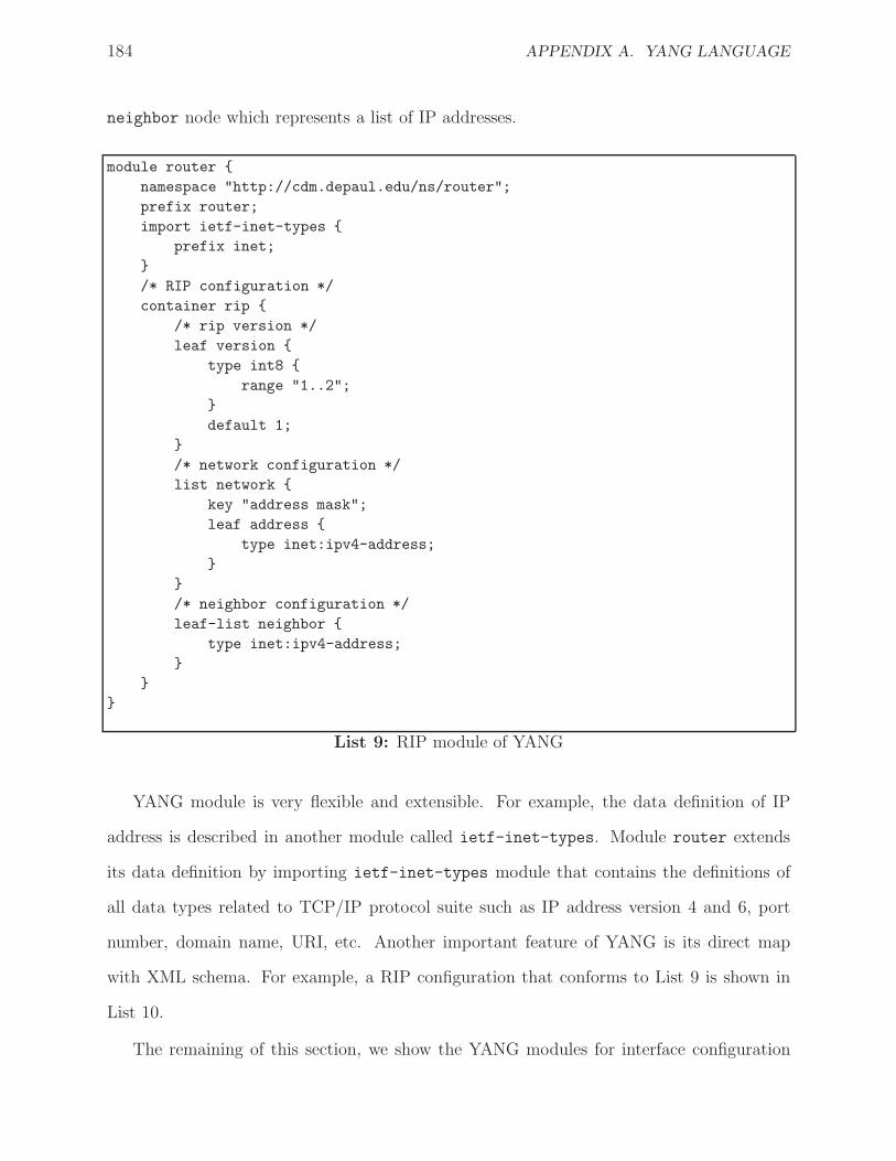
184 APPENDIX A. YANG LANGUAGE
neighbor node which represents a list of IP addresses.
module router {
namespace "http://cdm.depaul.edu/ns/router";
prefix router;
import ietf-inet-types {
prefix inet;
}
/* RIP configuration */
container rip {
/* rip version */
leaf version {
type int8 {
range "1..2";
}
default 1;
}
/* network configuration */
list network {
key "address mask";
leaf address {
type inet:ipv4-address;
}
}
/* neighbor configuration */
leaf-list neighbor {
type inet:ipv4-address;
}
}
}
List 9: RIP module of YANG
YANG module is very flexible and extensible. For example, the data definition of IP
address is described in another module called ietf-inet-types. Module router extends
its data definition by importing ietf-inet-types module that contains the definitions of
all data types related to TCP/IP protocol suite such as IP address version 4 and 6, port
number, domain name, URI, etc. Another important feature of YANG is its direct map
with XML schema. For example, a RIP configuration that conforms to List 9 is shown in
List 10.
The remaining of this section, we show the YANG modules for interface configuration
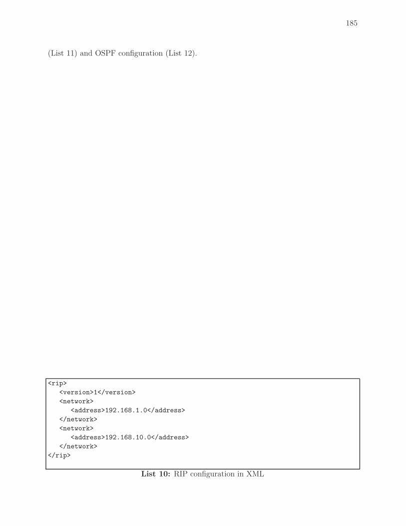
185
(List 11) and OSPF configuration (List 12).
<rip>
<version>1</version>
<network>
<address>192.168.1.0</address>
</network>
<network>
<address>192.168.10.0</address>
</network>
</rip>
List 10: RIP configuration in XML
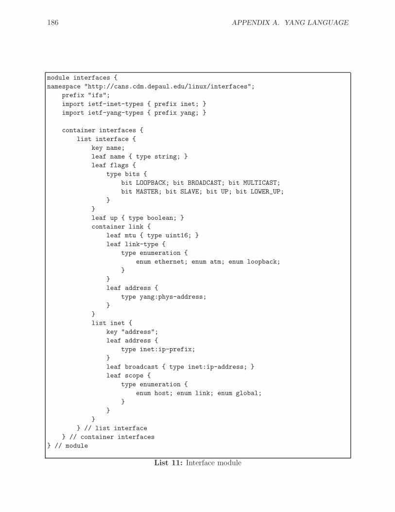
186 APPENDIX A. YANG LANGUAGE
module interfaces {
namespace "http://cans.cdm.depaul.edu/linux/interfaces";
prefix "ifs";
import ietf-inet-types { prefix inet; }
import ietf-yang-types { prefix yang; }
container interfaces {
list interface {
key name;
leaf name { type string; }
leaf flags {
type bits {
bit LOOPBACK; bit BROADCAST; bit MULTICAST;
bit MASTER; bit SLAVE; bit UP; bit LOWER_UP;
}
}
leaf up { type boolean; }
container link {
leaf mtu { type uint16; }
leaf link-type {
type enumeration {
enum ethernet; enum atm; enum loopback;
}
}
leaf address {
type yang:phys-address;
}
}
list inet {
key "address";
leaf address {
type inet:ip-prefix;
}
leaf broadcast { type inet:ip-address; }
leaf scope {
type enumeration {
enum host; enum link; enum global;
}
}
}
} // list interface
} // container interfaces
} // module
List 11: Interface module
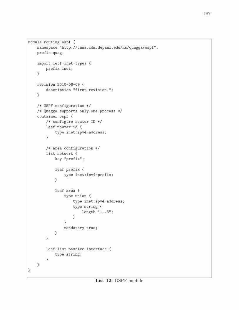
187
module routing-ospf {
namespace "http://cans.cdm.depaul.edu/ns/quagga/ospf";
prefix quag;
import ietf-inet-types {
prefix inet;
}
revision 2010-06-09 {
description "first revision.";
}
/* OSPF configuration */
/* Quagga supports only one process */
container ospf {
/* configure router ID */
leaf router-id {
type inet:ipv4-address;
}
/* area configuration */
list network {
key "prefix";
leaf prefix {
type inet:ipv4-prefix;
}
leaf area {
type union {
type inet:ipv4-address;
type string {
length "1..3";
}
}
mandatory true;
}
}
leaf-list passive-interface {
type string;
}
}
}
List 12: OSPF module


Appendix B
Structured Configuration Language
This appendix gives a description of SCL language.
B.1 Language Primitives
The language is typeless since the data constraints are enforced by Yang not SCL. The basic
data type in SCL is called term which can be a single value or a complex value. A complex
value is either a tuple enclosed by {} or a list enclosed by [].
SCL expresses the CSM model logically as a set of predicates. Each predicate has the
form {Q, x1, x2, ..., xn} where Q is the concept name and xi is an attribute value. For exam-
ple, the predicate {device, rtr01, ’area-one’, [router, abr]} means that rtr01 is a device that
has a parent device ’area-one’ and classified as a Router and Area Border Router(ABR).
The existence of single quotation mark in area-one is to indicate that area-one is a single
term; not the arithmetic expression (area− one).
B.2 SCL statements
SCL language has a set of statements. The general syntax of SCL statement is composed of a
command name followed by zero or more arguments followed by either a set of subcommands
189
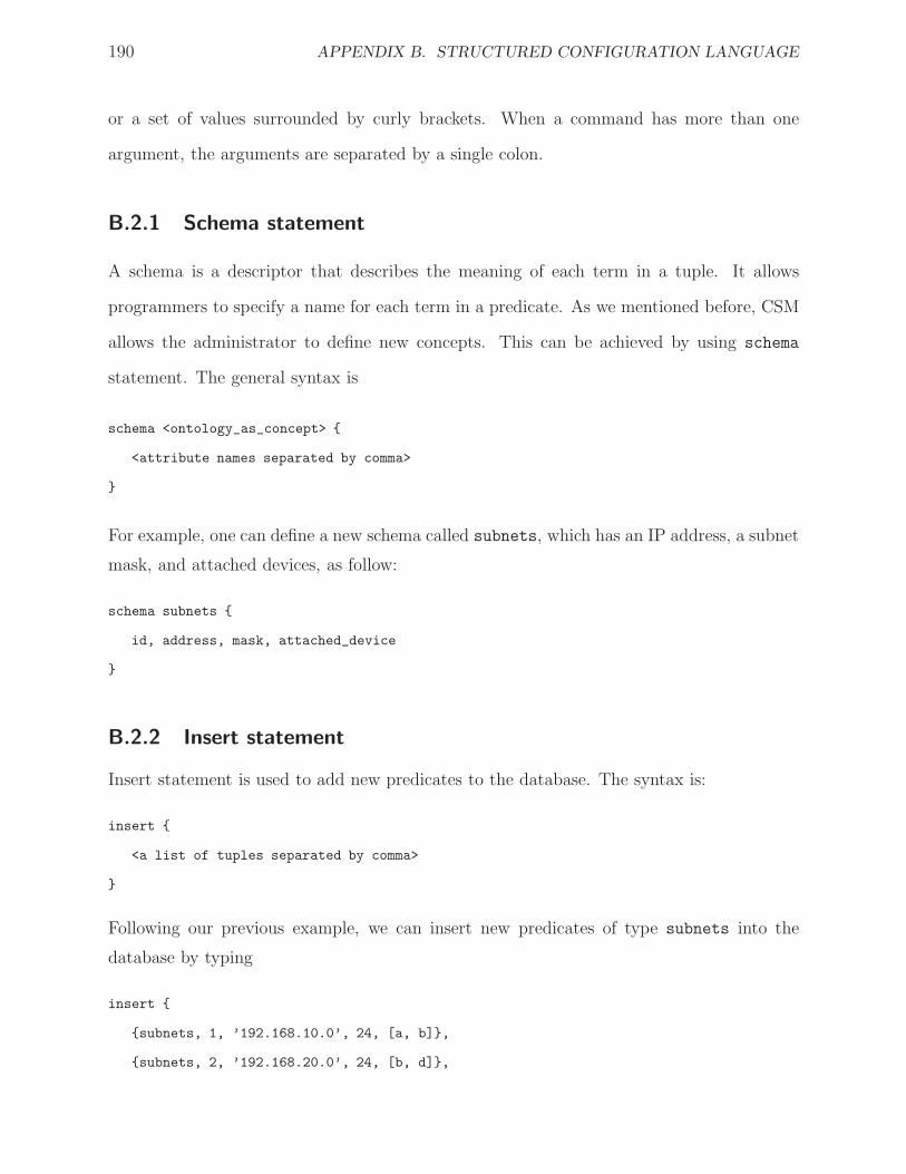
190 APPENDIX B. STRUCTURED CONFIGURATION LANGUAGE
or a set of values surrounded by curly brackets. When a command has more than one
argument, the arguments are separated by a single colon.
B.2.1 Schema statement
A schema is a descriptor that describes the meaning of each term in a tuple. It allows
programmers to specify a name for each term in a predicate. As we mentioned before, CSM
allows the administrator to define new concepts. This can be achieved by using schema
statement. The general syntax is
schema <ontology_as_concept> {
<attribute names separated by comma>
}
For example, one can define a new schema called subnets, which has an IP address, a subnet
mask, and attached devices, as follow:
schema subnets {
id, address, mask, attached_device
}
B.2.2 Insert statement
Insert statement is used to add new predicates to the database. The syntax is:
insert {
<a list of tuples separated by comma>
}
Following our previous example, we can insert new predicates of type subnets into the
database by typing
insert {
{subnets, 1, ’192.168.10.0’, 24, [a, b]},
{subnets, 2, ’192.168.20.0’, 24, [b, d]},
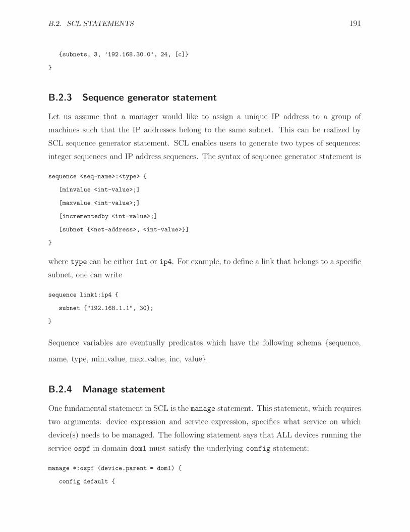
B.2. SCL STATEMENTS 191
{subnets, 3, ’192.168.30.0’, 24, [c]}
}
B.2.3 Sequence generator statement
Let us assume that a manager would like to assign a unique IP address to a group of
machines such that the IP addresses belong to the same subnet. This can be realized by
SCL sequence generator statement. SCL enables users to generate two types of sequences:
integer sequences and IP address sequences. The syntax of sequence generator statement is
sequence <seq-name>:<type> {
[minvalue <int-value>;]
[maxvalue <int-value>;]
[incrementedby <int-value>;]
[subnet {<net-address>, <int-value>}]
}
where type can be either int or ip4. For example, to define a link that belongs to a specific
subnet, one can write
sequence link1:ip4 {
subnet {"192.168.1.1", 30};
}
Sequence variables are eventually predicates which have the following schema {sequence,
name, type, min value, max value, inc, value}.
B.2.4 Manage statement
One fundamental statement in SCL is the manage statement. This statement, which requires
two arguments: device expression and service expression, specifies what service on which
device(s) needs to be managed. The following statement says that ALL devices running the
service ospf in domain dom1 must satisfy the underlying config statement:
manage *:ospf (device.parent = dom1) {
config default {
192 APPENDIX B. STRUCTURED CONFIGURATION LANGUAGE
...
}
}
The next example says that at least one device in domain dom1 running DHCP server must
satisfy the underlying configuration:
manage 1:dhcpsrv (device.parent = dom1) {
...
}
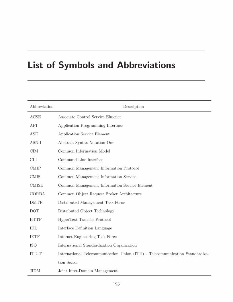
List of Symbols and Abbreviations
Abbreviation Description
ACSE Associate Control Service Elmenet
API Application Programming Interface
ASE Application Service Element
ASN.1 Abstract Syntax Notation One
CIM Common Information Model
CLI Command-Line Interface
CMIP Common Management Information Protocol
CMIS Common Management Information Service
CMISE Common Management Information Service Element
CORBA Common Object Request Broker Architecture
DMTF Distributed Management Task Force
DOT Distributed Object Technology
HTTP HyperText Transfer Protocol
IDL Interface Definition Language
IETF Internet Engineering Task Force
ISO International Standardization Organization
ITU-T International Telecommunication Union (ITU) - Telecommunication Standardiza-
tion Sector
JIDM Joint Inter-Domain Management
193

194 LIST OF SYMBOLS AND ABBREVIATIONS
Abbreviation Description
LLA Logical Layered Architecture
MIB Management Information Base
MO Managed Object
NE Network Element
NEF Network Element Function block
OO Object-Oriented
OS Operations System
OSF Operations System Function block
OSI Open System Interconnection
OSIE OSI Environment
PDU Protocol Data Unit
QoS Quality of Service
RDL Resource Definition Language
ROSE Remote Operation Service Element
RPC Remote Procedure Call
SDH Synchronous Digital Hierarchy
SLA Service Level Agreement
SMAE System Management Application Entity
SMASE System Management Service Element
SMI Structure of Management Information
SNMP Simple Network Management Protocol
SOAP Simple Object Access Protocol
SQL Structured Query Language
TF Transformation Function block
TMF TeleManagement Forum
TMN Telecommunication Management Network
WBEM Web-Based Enterprise Management

195
Abbreviation Description
WS Workstation
WSF Workstation Function block
XML Extensible Markup Language
XSL Extensible Styesheet Language
XSLT XSL Transformation