TOWARDS A UNIFIED THEORY OF CAPITALIST DEVELOPMENT*

Adolfo Figueroa

Economics Department Catholic University of Peru

Lima, April 2006 afiguer@pucp.edu.pe

Abstract. Since the 1950s, the capitalist world economy has shown significant empirical regularities, which can be characterized by the existence and persistence of (1) differences in income levels between the First World and the Third World, (2) differences in the degree of inequality between the First World and the Third World, (3) unemployment and underemployment across these group of countries. Standard economics has not been totally successful in explaining these facts. A possible reason for this failure is that standard economics assumes a homogeneous world capitalism in which countries differ only in quantitative aspects, such as factor endowments, saving rates, population growth rates, and technological diffusion rates. This paper presents a new theoretical approach in which three types of capitalist societies are assumed, each with different initial conditions in terms of factor endowments and the degree of inequality in the individual endowments of economic and social assets. Another critical assumption is that labor markets operate as non-Walrasian markets. The empirical predictions of the partial theories (for each type of society) and the corresponding unified theory of capitalism are then confronted against the observed empirical regularities. These facts appear to be consistent with the predictions of the theories. I. Introduction

The science of economics has remarkably developed in recent times. It has supplied societies with a significant core of knowledge. However, it has been unable to satisfy all the existing demand for knowledge. Many fundamental questions still remain unanswered, as will be pointed out below. Therefore, the supply of knowledge needs to be increased. This paper intends to be a contribution to that objective. Economics, as a factual science, needs to establish a set of fundamental factual regularities, which will then become the scientific puzzles to be explained. The empirical regularities about production and distribution in the capitalist world economy over the last five to six decades can be summarized as follows:

First World: 1. The existence and persistence of unemployment. The US economy, for instance, shows a mean unemployment rate of 6% in the period 1948-1996 (Barro 1997, Table 10.2, p. 366). This rate varies by countries, but what is certain is the fact

* A shorter version of this paper was submitted to the 2005 Global Development Awards Competition of the Global Development Network and was selected as a medal finalist in the category “Globalization, Institutions, and Development” of the Medals for Research on Development . A first draft was presented at the International Conference on Globalization, Inequality, and Poverty, organized by the Economics Department, University of Utah, Salt Lake City, November 18-19, 2004.

2

that it is always positive (ILO, World Unemployment Report, annual). Unemployment may be considered the disease of capitalism, as stated by the well-known historian John Garraty (1978). Third World: 2. The existence and persistence of unemployment and underemployment. Underemployment is defined as the self-employed workers making incomes at a rate that is lower than the market wage rate, for comparable skills. Thus, underemployment is a form of excess labor supply, in addition to unemployment. The fact is that the underemployment rate is the most significant, around 50%, in most Third World countries, while unemployment rates are not much different from those observed in the First World (ILO World Development Report, annual). 3. Inequality between ethnic groups is significant and persistent. In the account of overall inequality of these countries, ethnicity matters. Thus, poverty incidence is higher in particular ethnic groups. There are several empirical estimates on the income gap between dominant and subaltern ethnic groups in countries of Latin America, Africa, and Asia (Darity and Nembhard 2000, Hall and Patrinos 2005, Psacharopoulos and Patrinos 1994, Silva 2001, Stewart 2001).

World Capitalism: 4. There is interplay between nominal and real variables in the short-run. The US economy shows that monetary aggregates are procyclical (they move in the same direction of output) based on quarterly data from 1959 to 1996 (Barro 1997, Table 18.1, p. 705). Money aggregates have also been found to be procyclical in a sample of 15 countries of the Third World and 10 of the First World for the period 1970-1997 (Rand and Tarp 2002). Thus, changes in nominal variables are positively correlated with the level of economic activity. 5. In the long run, real wages rise as total output or output per capita grows. A well-known textbook in macroeconomics states, “This proposition accords with data for a large number of countries” (Barro 1997, p. 225). 6. Income level differences persist between the First World and the Third World. The growth rates of output per capita in the Third World countries are not higher than the corresponding rates in the First World countries. Hence, there is no tendency to convergence in per capita income levels between these two groups of countries. This empirical observation comes from a sample of 114 countries of the world economy in the period 1960-1990 (Barro 1997, Figure 11.10 and Table 11.3, pp. 412-413). The statistical test is abundant in the literature (cf. Barro and Sala-i-Martin 1995, Sala-i-Martin, Doppelhofer, and Miller 2004). 7. Differences in the degree of inequality also persist between the Third World and the First World countries. This evidence comes from a study of the World Bank based on a sample of countries of the world economy in the period of 1950-1995, for a total of 682 observations (Deninger and Squire 1996). The statistical test on the constancy or mild increase of inequality in most countries is presented in Li, Squire, and Zou (1998).

Neoclassical economics can explain some of these facts, but not all. In particular, it ignores fact 7 and presents the hypothesis of “conditional convergence” regarding fact

3

6. To test this hypothesis, cross country regression analysis is applied through the “inclusion of variables that proxy for differences in steady state positions” (Barro and Sala-i-Martin 1995, p. 30); however, the refutation of the theory by testing its reduced form relations is not pursued. In addition, the assumption of steady state equilibrium has been put into question. Thus, Robert Solow (2001) has said: “The exponential steady state is a theoretical convenience. But many countries, much of the time, are no where near steady-state growth. This suggests that comparative studies should focus less on the growth rate and more on comparing and understanding whole time paths” (p. 288). This study takes into account Solow’s suggestion. The theoretical framework proposed here assumes the existence of different types of capitalist economies, which differ in their initial conditions and then in their consequent time paths. These partial theories will then attempt to explain the First World and the Third World economies separately. The emergent unified theory attempts to explain capitalism as a whole and makes the partial theories appear as models of this general theory. Thus this theoretical framework seeks to explain facts 1 to 7. The general theory is presented in section II. The static models are presented in sections III and IV. A theory of investment appears in section V, the dynamic models in section VI, and the conclusions in section VII.

II. The General Theory: Primary Assumptions The general theory assumes that there are different kinds of capitalist economies. They all have, however, common features that can be established theoretically. This general theory can then be expressed as the following set of primary assumptions, called alpha propositions:

α1. Institutional context. (a) Rules: People participating in the economic process are endowed with economic and social assets; economic assets are subject to private property rights; market and democracy constitute the basic institutions of capitalism, which operate with mechanisms of social inclusion and exclusion at the same time; people exchange goods subject to the norms of market exchange, which include the norm that nominal wages cannot fall; (b) Organizations: Firms, households, and a democratic government exist. α2. Initial conditions. Individuals are endowed with unequal quantities of economic and social assets. There are two social classes: capitalists and workers. α3. Economic rationality of agents. Individuals behave guided by the motivation of self-interest. Capitalists seek two objectives that are hierarchically ordered: maintenance of the social position and profit maximization. In the labor market, workers seek to maximize wages and minimize effort. The class division of society generates social conflict in the sense that workers are not full partners with capitalists and that capitalists must use devices to extract work effort from workers. Capitalists prefer profits to rents. People in government also act guided by self-interest; they seek political power, with the ultimate goal of income maximization. α4. Social tolerance to inequality. Individuals have a sense of justice about their absolute and relative wealth in society; that is, they have a limited tolerance to economic inequality. If inequality reaches values that go beyond the threshold of

4

tolerance, individuals will react and seek to reduce the excessive inequality by breaking the rules of the institutional context.

These assumptions make up the hard core of a general theory of capitalism. Within that core, capitalism can take different forms, which will be explained by models of the general theory. Three types of capitalist societies are assumed in this study. These societies differ only in the initial conditions under which they were born to capitalism. Two factors constitute the initial conditions. One refers to the well known factor endowment: the capital-labor ratio; the other is the initial degree of equality in the individual endowments of economic and social assets, which will be called the equality endowment. These two types of endowments will determine different initial institutional contexts under which capitalism will operate; consequently, different outcomes of production and distribution will emerge. These abstract societies are called sigma, omega, and epsilon. Sigma is born as overpopulated and highly unequal, omega as overpopulated and mildly unequal, and epsilon as unpopulated and the least unequal. Economic assets include several forms of capital: physical, financial and human. Physical and financial forms of capital are highly concentrated in a particular social group, the capitalists. Workers are endowed with different quantities of human capital.

Social assets will include political and cultural assets. Social factors are thus introduced into the economic process, which requires the transformation of social factors into goods, as resources or assets that people are endowed with. Certainly, social assets will be special goods for they are in the realm of people’s rights and entitlements in society; that is, they are neither physical goods, nor are they marketable. Political assets are defined as the capability of exercising individual and collective rights, including the right to have access to rights. Inequality in the endowment of political assets generates a hierarchy of citizens in society, first-class and second-class citizens. As a result, not all individuals are equal before the law; not all individuals have the same access to public goods supplied by the state.

Cultural assets are defined as the right of groups of individuals to cultural diversity in a multiethnic and multicultural society. Inequality in the endowment of cultural rights generates a hierarchy of ethnic markers in society: there are first-class and second-class races, languages, religions, and customs. These assets are cultural because this hierarchy is socially learned and transmitted from generation to generation. Inequality in cultural assets leads to social practices of segregation, exclusion, and discrimination against some ethnic groups, which reinforces unequal citizenships.

Why would inequality in social assets exist? Inequality in the endowments of social assets implies the dominance of some ethnic groups by others. This domination system may be the result of the foundational episode of society (a war or a conquest). This foundational shock generates a multiethnic and multicultural society, and a hierarchical one. All are class societies, in the sense that economic assets are unequally distributed. Sigma, however, shows inequality also in social assets; it is a socially heterogeneous and hierarchical society, in which citizenships differ among individuals. Omega and epsilon are socially homogeneous, equal-rights societies.

5

II. Sigma Economy: A Highly Unequal Society

A. A Static Model of Sigma Theory In order to derive empirically refutable predictions from sigma theory, a model of this economy must now be established, which implies the introduction of some consistent auxiliary assumptions. There are three ethnic groups: the Blues, the Reds, and the Purples (mestizo people).1 They are endowed with one of the three hierarchical levels of citizenship: A, Y, Z, in that order. There are two social classes: capitalists and workers; Blues are the capitalists and the others are workers. There are two levels of human capital, skilled and unskilled; Blues and Purples are skilled, but Reds are unskilled. These are the initial endowments. Social classes and ethnic groups make up the social structure of sigma society. Ethnic groups will be called by their citizenship status (social groups A, Y or Z) because this is the endowment the theory is concerned with and because there is one-to-one relationship between these two categories. In this sense, sigma is clearly a highly correlated society Given these initial conditions, how production and distribution would be determined in this economy? Would the initial inequality in the endowment of individual and collective assets tend to remain or to diminish endogenously? “Y-workers” supply their labor to the labor market, which is non-Walrasian. The labor market operates with excess labor supply, the quantity of which is determined endogenously. This quantity is, in part, self-employed in small units in the y-subsistence sector and, in part, to unemployment.

“Z-workers” are endowed with low human capital for the technology being used in the capitalist sector. Thus, their human capital endowments are not suitable for wage employment. They are not employable; therefore, they are not part of the labor supply in the labor market. Capitalist firms cannot make profits employing them, as there would be much need to invest in their training, when at the same time y-workers are in plentiful supply. It is the lack of profitability that lies behind the total exclusion of z-workers from the labor market. Z-workers conform to the definition of the underclass: workers “who are largely expendable from the point of view of the logic of capitalism” (Wright 1997, p.28). They are self-employed in small units in the z-subsistence sector. Three sectors therefore constitute the economic structure of sigma economy: the capitalist sector, the y-subsistence sector, and the z-subsistence sector. This is a one-good economy; that is, the same good B is produced in each sector. The level of labor productivity is highly differentiated between these sectors: the capitalist sector shows the highest level, followed by the y-subsistence sector, and finally the z-sector. This order reflects differences in capital (physical and human) endowments and technological knowledge between capitalist firms and subsistence units. It is assumed that a threshold of human capital is needed to learn the technology used in the capitalist sector. It is also assumed that z-workers are endowed with human capital that is below this threshold. 1 In a paper that analyzes the theoretical relationships between consumer preferences and culture, Akerlof and Kranton (2000) construct an abstract world of two ethnic groups, the Greens and Reds, in which the Greens are the dominant group. To use primary colors, call them Blues and Reds here; then introduce a third ethnic group: the Purples, the result of miscegenation of the two races. As in that paper, it is assumed here that people cannot choose their ethnic identity; ethnicity is exogenous.

6

Production in the subsistence sectors is for direct consumption by the producer rather than for the market. Subsistence units are, therefore, production and consumption units at the same time. Labor productivities in the subsistence sectors are too low to allow wage employment and the generation of profits. The market system contains four markets: good B, labor (H), money (M), and foreign exchange (E). The labor market is non-Walrasian, but the others are Walrasian. All markets operate under conditions of pure competition. The economy is static and open. Good C is an imported input utilized to produce good B. This sigma economy is assumed to be very small in international trade; so international prices are exogenously given. Hence, in equilibrium the domestic price of commodities B and C, measured in units of the domestic money, are equal to:

Pb = Pe Pb

* (1) Pc = Pe Pc

* Here Pe is the nominal exchange rate and Pb

* and Pc* are international prices

denominated in units of the foreign exchange. Each domestic price must be equal to the international price multiplied by the nominal exchange rate. If this equality did not hold, people would buy commodity B from the cheaper source and sell it wherever the price is higher. The ratio z* = Pb

*/Pc* is the international terms of trade.

Firms produce good B under the logic of seeking the maximization of nominal profits (P’). For firm j, this rationality can be represented as follows: Maximize Pj’ = Pb Qbj - Ph Dhj - Pc Dcj (2)

Subject to Qbj = λ Φj (Dhj, Kbj, δ), Φ1>0, Φ11<0, Φ2>0, Φ3<0 Qbj = Dcj /n Xbj = (1/z*) Dcj

w ≥ w*= (1+c) v’ implies λ=1, otherwise λ=0.5

In this system, Qbj is the firm’s total output, Dhj is the quantity demanded of labor, Dcj is the quantity demanded of input C, Ph is the nominal wage rate and w is the real wage rate, and finally n is a technological coefficient, the quantity of good C required to produce one unit of good B. Technology is subject to constant returns to scale and diminishing returns. Information about technology is a public good, but the production function is specific to each firm due to differences in entrepreneurial talents and in the cost of access to public goods and natural resources. The consequence is that individual demand curves for labor differ by firms and that profits, given market wage rates, can be positive (and unequal among firms) even under competitive markets. The production function is subject to limitational factors and is thus represented as a system of equations. Inequality in the individual endowment of assets δ also enters into the firm’s production function. For a given quantities of the other inputs, its effect is negative because a higher degree of inequality generates an environment of higher degree of social disorder, which in turn increases transaction costs and property protection costs in the economy. Therefore, a higher degree of inequality leads to higher degree of inefficiency in the economy.

7

The third constraint indicates that the firm must use part of its output to export, Xbj, so as to import input Dcj. The last constraint indicate that the firm must pay real wages that are higher than the opportunity cost of workers, which is a premium above the marginal productivity of labor in the y-subsistence sector v’. This is the device firms use to discipline workers—for simplicity, only two degrees of work effort (λ) are considered. Symbol w* indicates the lower limit of the range of efficiency wages. The firm’s equilibrium condition is the following:

Φj1 (Dhj, Kbj, δ) (Pb – n Pc) = Ph (3)

Φj1 (Dhj, Kbj, δ) (1 – n/z*) = w, where (n/z*) < 1, and w≥ w* Pb Sbj = (Pc Dcj – Pb Xbj) + Ph Dhj

The marginal productivity of labor is net of the cost of using the limitational input C. The first equation shows the labor demand curve in terms of the nominal wage rate and the second in terms of the real wage rate. Hence, the quantity demanded for labor depends also on the terms of trade. The third equation is the firm’s budget constraint, where Sbj is the quantity of good B supplied to the market. The equilibrium situation indicated in the system (3) is stable and unique; hence, comparative statics can be applied to determine empirical predictions for behavior at the firm level. The firm’s labor demand function can then be derived from (3), which would indicate that the price of good B and the stock of capital have a positive effect, whereas the price of good C and the nominal wage have a negative effect. The quantity of good B supplied to the market is derived from the firm’s budget constraint. Aggregating over all firms, the behavior of capitalists in the labor market can be written as the following system of equations: Dh = H (Pb, Pc, Ph, Kb, δ), where H1>0, H2<0, H3<0, H4>0, H5<0 (4) Subject to

Pb Sb = Pb Qb – PbXb – P’ = (PcDc – PbXb) + PhDh Xb = (1/z*) Dc = f (Dh, Kb, δ, z*) where f1>0, f2>0, f3<0, f4<0 w ≥ w* = (1+c)v’ and Ph ≥ Ph

*

The first equation is the labor demand function. The second equation shows the quantity of good B supplied to the market (Sb), which also represents the firms’ budget equations. The third equation represents the exports function. The last constraints indicate that wages must belong to the set of efficiency wages and that nominal wages cannot fall below its current value Ph

*. Under a system of flexible exchange rates, in a one-good economy, a particular rule for the functioning of the foreign exchange market can be assumed: firms export commodity B and get foreign exchange, which they sell to the central bank and get domestic currency; then firms use domestic money to buy back foreign currency, which they use to import commodity C. Transaction costs in these operations are zero. The rate of exchange is flexible; so this market is Walrasian. In this particular model, the equilibrium of the foreign exchange market is determined by the behavior of firms alone. Given the stock of capital, a level of employment will produce a given amount of good B. Because input C is limitational, this output will not be obtained unless a determined amount of input is imported, which is paid with exports by the firms themselves. Thus, there is no need for any mechanism

8

of coordination. This is what the third equation of the system (4) shows. The labor demand function is such that for every nominal wage there is a quantity demanded for labor, which produces a quantity of net output, net of exports needed to pay for the required imported input; that is, every point on the labor demand curve implies equilibrium in the foreign exchange market. From the firms’ budget constraints, the following relations then hold true:

Pc Dc = Pb Xb (5)

Pc* Dc = Pb

* Xb The first equation shows that firms pay with exports for their required imports. The second equation indicates the corresponding equilibrium in the foreign exchange market. This equilibrium is independent of the value of the exchange rate; that is, it holds true for any value of Pe. On the behavior of y-workers, assume that they are endowed with quantities of money. They have transactions demand for money because they sell their labor and get paid at the end of the production period. The rest of the agents are not required to have money balances. Capitalists pay wages at the end of the production period, and profits are just taken out of output. The self-employed in the subsistence sectors produce for the direct consumption by the producers. The behavior of the individual worker j can be represented by the following system of equations:

Ph Dhj = Pb Dbj + (Smj – Dmj) (6)

Dmj = Pb Lj (Dbj), where Lj’>0, Lj’’<0 Smj – Dmj = Pb dbj

The first equation shows the worker’s budget constraint, which says that the worker allocates his income to the purchase of good B and to the restoring of his required cash balance. His income is equal to the nominal wage rate multiplied by the quantity of labor bought by firms, not multiplied by his supply of labor. This is so because the worker participates in a non-Walrasian labor market, where the rationing mechanism is assumed to be random. The second equation refers to the cash balance constraint: the higher the income, the higher the cash balance to be held for transactions purposes, however less than proportional. The third equation refers to the adjustment mechanism to restore the required cash balance. Any cash balance in excess is spent in good B (the term Pb dbj) and any shortage is restored purchasing a smaller amount of good B, where this adjustment is made in one period. The equilibrium condition is dbj =0. In the aggregate, the market behavior of wage earners can be written as follows: Db = F (Pb, Dh, Ph), where F1<0, F2>0, F3 >0 (7)

Dm = Pb L (Db) = Pe Pb*

L (Db), where L’>0, L”<0 Subject to

Ph Dh = Pb Db + (Dm – Sm)

The first equation shows the demand function for good B and the second one the demand function for money. The last equation is the workers’ budget constraint.

9

B. The General Equilibrium Solution There are three Walrasian markets and one non-Walrasian market (labor), where equilibrium is consistent with excess labor supply. Thus, the general equilibrium conditions can be written as follows: Labor market Sh > Dh (8)

Good B market Sb = Db Money market Sm = Dm Foreign exchange Pb

* Xb = Pc* Dc

Subject to the aggregate budget constraint Pb (Db – Sb) + Pe (Pc

* Dc - Pb* Xb) + (Dm – Sm) = 0

Because the equilibrium condition of the foreign exchange market is already incorporated in the labor demand function, the two remaining Walrasian markets together with the labor market need to be solved. The aggregate budget constraint gives rise to Walras’ law: one of the Walrasian markets is redundant. Let the commodity market be the redundant one. Thus, in order to get general equilibrium it is sufficient to solve a system of two markets only: the money market (a Walrasian market) and the labor market (a non-Walrasian market). From the systems (1), (4) and (7), the following system is obtained: Dh = H (Pe; Ph, Kb, δ, z*), where H1>0, H2<0, H3>0, H4<0, H5>0 (9)

Sm = Pe Pb* L (Db) = M (Pe, Dh; Ph, Pb

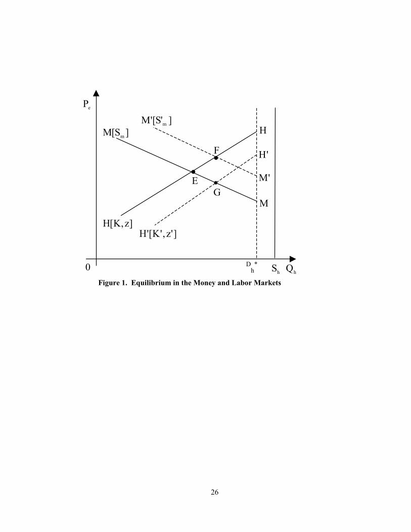
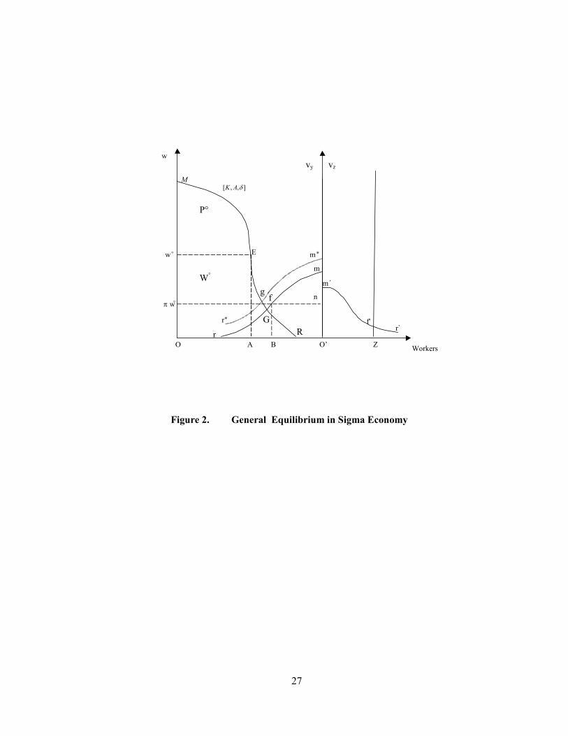
*), where Mi>0, all i. These two equations should solve for two endogenous variables, the exchange rate Pe and the level of employment Dh. The solution of this system is simultaneous. The solution is shown in Figure 1. The upward sloping curve HH represents the set of combinations of exchange rate and employment level that are consistent with the equilibrium in the labor market. The higher the exchange rate, the higher the domestic price level, and consequently the higher the employment level will be. The downward sloping curve MM represents the set of combinations of exchange rate and employment level that clear the money market. The higher the employment level, the higher the required real cash balances, the lower the domestic quantity demanded of good B, the higher the supply of foreign exchange and the lower the exchange rate will be. Hence, the set of values of exchange rate and employment level that is consistent with equilibrium in both markets is determined by the intersection of both curves, at point E. Once Dh is known, total output can also be known, and Dc is technologically determined. Then the quantity of exports Xb is determined, as firms must pay for the quantity of imports of intermediate commodity C at the given terms of trade. Thus equilibrium is assured in the foreign exchange market. Total output in the capitalist sector is net of the quantity of exports needed to pay for the imports of intermediate goods. Because the nominal exchange rate is known, the domestic price level is also determined, and so is the real wage rate. The general equilibrium of production and distribution in the entire economy is presented in Figure 2. In the capitalist sector, the interactions of money and labor markets determine the equilibrium values of real wage (w°) and wage employment (the segment OA), which is represented by point E on the labor demand curve MER. Money

10

and labor markets are in equilibrium at point E. At this point, the foreign exchange market is also in equilibrium because, by construction, in every point on the labor demand curve the equilibrium in the foreign exchange market is assured. By Walras’ law the market for good B should also be in equilibrium, which can be seen graphically if one realizes that the quantity supply to the market—equal to total output minus profits—is the same area as that of the real wage bill, which in turn is equal to the quantity demanded for good B. The resulting excess labor supply is equal to the segment AO’, where OO’ is the total quantity supplied of y-workers. The labor marginal productivity curve in the subsistence sector (curve mr, read from origin O’) shows diminishing returns and is placed at a lower level than the corresponding curve in the capitalist sector because of the assumption of lower productivity. This curve also represents the labor supply curve (read from origin O). At a given market real wage, workers have the choice to take either employment in the labor market or become self-employed. Workers that can earn a higher income as self-employed will choose not to enter the labor market. If the wage rate rises, fewer workers will take this decision (due to diminishing returns) and more workers will shift to seek wage employment. Hence, the curve mr represents the labor supply curve. If the market real wage were determined where supply and demand curves cross each other, the equilibrium situation would be at point G. This would imply that the labor market is Walrasian. But the labor market could not operate in this manner because work intensity would be lower (λ=0.5), and then the labor marginal productivity curve would shift downward and profits would be smaller. The effort extraction curve is obtained by shifting upward the supply curve by a factor (1+c), where c is a positive number and operates as a premium paid to wage earners. This is shown as the m*r* curve in Figure 2. As long as this gap prevails, the degree of effort will be at maximum (λ=1), and the labor demand curve will remain in the same position. This gap will operate as a restriction for wage determination. Given the effort extraction curve and the labor demand curve, there is a minimum value of the set of efficiency real wages, w*=(1+c) v’, which is determined where these curves cross each other (point g). This minimum efficiency wage also implies a maximum level of wage employment (Dh

*). The incentive system leads y-workers to seek wage employment, but jobs are unavailable for all workers, no matter how hard each worker seeks. Because a turnover of workers is common in the capitalist sector due to dismissals of those workers found shirking, a given probability of finding a job in that sector exists. Given that the mechanism of rationing is random (assumed above), this probability will be the same for all workers. Let we represent the workers’ expected wage when seeking a job. For an exogenously given probability π to find a job, the expected wage depends positively on the market wage rate. These assumptions imply a uniform expected wage for all workers, which can be written as: we = π w, where 0 < π < 1 (10)

As the ‘second best’ solution, the workers who are excluded from wage employment will choose between unemployment and self-employment. These workers will evaluate the expected wage when they engage in the activity of job seeking (and become

11

unemployed) against the sure income they can make in the subsistence economy. If the expected real wage rate is higher than the sure income in the subsistence economy, these workers will decide to seek a wage income and will become unemployed. If the expected real wage rate is lower, they will choose self-employment in the subsistence sector. Because the expected wage depends upon the market wage rate, the higher the wage rate the higher the proportion of the excluded going to unemployment and thus the lower the proportion going to self-employment, for a given level of excess labor supply. The output and employment of equilibrium in the y-subsistence sector is obtained from the following system: Eh° = Ly + U (11)

Qby = J (Ly), where J’>0, J”<0 πw° = J’ (Ly),

The first equation indicates that the excess labor supply (Eh

o) is allocated to self-employment (Ly) and unemployment (U). The second equation is the production function in the subsistence sector (where abstraction is made of imported inputs). The equilibrium condition for the allocation of labor to self-employment is established in the third equation. This equation determines the level of self-employment and total output in the y-subsistence sector. Unemployment is residual. This solution is also shown in Figure 2. Once the wage rate is known, the expected wage is determined. This is marked as a fraction of the market wage rate. This value must be equal to the marginal productivity of labor, which occurs at point f and determines employment and output in the y-sector; unemployment is then residual. Thus, the allocation of the excess labor (AO’) to unemployment (AB) and self-employment (BO’) is solved. The gap between the real wage and the marginal productivity of the total self-employed labor must satisfy the condition that the difference must be equal to or higher than the premium needed to assure labor discipline. At point B, the equilibrium real wage is indeed above the curve m*r*. If this condition were not met, workers would have incentives to shirk and profits would be lower; hence, firms would seek to increase the nominal wage rate in order to increase the real wage rate and maintain work intensity, and thus profits. The labor market is thus a non-Walrasian market, where equilibrium is achieved with excess labor supply. Some workers are willing to exchange their labor at the market real wage, but are not able to do so. Unemployment is the result of economic choice made by those workers who are excluded from the labor market. This unemployment is ‘voluntary’ in the sense that it is the result of economic choice. But it is involuntary in the sense that, at the prevailing market real wage rate, this is not the most preferred situation for workers. Unemployment or self-employment is a choice in a second best situation.

In the z-subsistence sector, the quantity of workers Shz is exogenously given. Workers seek to maximize (individually or collectively) total output in their units of production. The implicit rule of distribution is that each worker gets the average productivity of labor. Income differentials among z-workers are due to inequality in resource endowments. The equilibrium condition is simply Vz = f ( Lz ), f’>0, f”<0 (12)

12

Shz = Lz where Vz is the total output of the sector and Lz is total self-employment. Because there is no interaction between the z-subsistence sector and the capitalist sector, the general equilibrium is separable. The general equilibrium in the sigma economy is sequentially determined. First, equilibrium in the capitalist sector is determined. The solution of the y-subsistence sector follows the market solution. Unemployment of y-workers is then residual. Solution in the z-subsistence sector is determined independently of the rest of the economy. Total output of equilibrium (or national income of equilibrium) is also shown in Figure 2. In the capitalist sector total output is equal to the area under the curve ME, in the y-subsistence sector total output is equal to the area under the curve mf, and in the z-subsistence sector total output is equal to the area under the curve m’f’. The sum of these three areas makes up total output of equilibrium. National income (Y) of equilibrium and its distribution by social groups (where y-workers and z-workers are explicitly distinguished) can be represented by the following system of equations: Y = P + Wy + Vy + Vz (13)

= P + wy Dhy + vy (Ly + Uy) + vz Lz Shy = Dhy + Ly + Uy

Shz = Lz Profits (P), wage bill (Wy), and total income in the two subsistence sectors (Vy and Vz) will compose national income. Labor incomes can be broken down into mean incomes (wy, vy, vz) and quantities of workers in each social group. The term vy measures the mean income of the y-workers who are excluded from the labor market, the excess labor supply. This social group has a mean income that is lower than the wage rate (wy>vy) because this is the condition for the functioning of the capitalism in an overpopulated economy. Inequality in the endowments of physical capital and human capital among sectors leads to the following relation in the mean income of workers: wy>vy>vz. The z-workers will constitute the poorest group in society.

C. Comparative Statics

The static general equilibrium presented above indicates that national income and its distribution in sigma economy will be repeated period after period as long as the exogenous variables remain fixed. The equilibrium in the capitalist sector is clearly stable, as can be seen in Figure 1. Comparative statics can thus be applied to derive empirical predictions: the effect of changes in the exogenous variables upon total income and its distribution. The exogenous variables of the system include the quantity of money (a parameter in the MM curve), the capital stock and the terms of trade (parameters in the HH curve) and the labor supply. There exists a maximum level of employment Dh

* in the labor market. Consider the case when the initial equilibrium occurs in the range of Dh<Dh

*.

13

The effect of an increase in the money supply is positive upon both the exchange rate and the employment level in the capitalist sector. In Figure 1, curve MM shifts upwards and the new equilibrium is at point F, which implies a higher exchange rate and a higher employment level. As money supply increases further, the level of wage employment will continue to increase, and eventually will reach the level L*. More money supply will now have the effect of raising prices and nominal wage only leaving unchanged the real variables. Thus, this model predicts ‘money neutrality’ after the threshold of maximum wage employment. An increase in the terms of trade will shift the curve HH outwards, and the new equilibrium will occur at point G, which implies a higher employment level and a lower exchange rate. The effect of an exogenous increase in the capital stock is positive on the equilibrium value of employment in the capitalist sector and negative on the equilibrium value of the exchange rate. In Figure 1, the HH curve shifts outwards, now as a result of an increase in the capital stock, and the new equilibrium is at point G. This result implies that an increase in the terms of trade is equivalent to an increase in the capital stock of the economy; vice-versa, a fall in the terms of trade is equivalent to a destruction of the capital stock. However, the terms of trade effect should be seen as short run and the capital accumulation effect as long run. These empirical predictions imply that in a static-open model, where investment is exogenous, the z-subsistence sector can neither be affected by nor affect the capitalist sector. This model predicts economic dualism between the capitalist sector and the z-subsistence sector, but growth of the capitalist sector affects positively the y-subsistence sector. Capital accumulation in the capitalist sector has no effect on the z-subsistence sector because it does not affect employment; z-workers are all excluded from the labor market. It does not affect the productivity curve either because z-workers lack the stock of human capital needed to adopt these new capital goods and technologies. There is ‘trickle down’ effect on the y-subsistence sector, but not on the z-subsistence sector. The effect of changes in exogenous variables upon income inequality is ambiguous. Looking through the components of the Lorenz curve, changes in income inequality depend upon changes in two critical ratios: relative mean incomes and relative population shares of social groups. But the exogenous variables affect these ratios in directions that are either ambiguous or offsetting. Take the case of capital accumulation. In the capitalist sector, both total profits and the wage bill increase, but their shares in national income are undetermined. Total income in the y-subsistence sector falls, which implies a fall in its share in national income, but average income rises. The income share of z-workers falls. In addition, the proportion of y-workers in total labor force falls and the proportion of wage earners increases, but changes in the relative mean incomes change are unclear. The new Lorenz Curve might get shifted slightly outward or inward, or it might cross the initial curve. In any case, overall inequality cannot change much. IV. Omega and Epsilon Economies

Consider now omega society. This is a socially homogeneous society, in which individuals are all first class citizens. Even if ethnic groups existed, this would be an equal-rights society; that is, social groups A-Y-Z do not exist. Omega is, however, a class society. All workers are skilled. In terms of the economic structure, omega

14

economy is composed of the capitalist sector and a subsistence sector, which is the result of overpopulation. This is just the sigma economy without the z-subsistence sector. The general equilibrium of this economy has already been solved. The epsilon economy is socially homogeneous and non-overpopulated. In terms of the economic structure, the epsilon economy is constituted by a capitalist sector alone. Therefore, the epsilon economy is just the omega economy without the subsistence sector. The work effort extraction device could not then be based on the opportunity cost of workers given by the income in the subsistence sector. It is assumed here that the device is based on a minimum rate of unemployment u*, which may be translated into a minimum real wage rate w*; that is, those found shirking will suffer the cost of becoming unemployed (Shapiro and Stiglitz 1984, Bowles 1985). The general equilibrium solution in epsilon has already been solved; it was shown above that the general equilibrium of omega economy was sequential, the capitalist sector being solved firstly. The only difference is that the efficiency wage threshold is determined by the unemployment rate of efficiency, which is exogenously determined. The epsilon economy can also be represented in Figure 2. Disregard the two subsistence sectors and let the quantity of labor supplied be represented by the segment OB. The mechanism of effort extraction in this case is given by the minimum rate of unemployment (u*), which determines the maximum level of wage employment. Let this level fall somewhere between points A and B. Let the equilibrium in the capitalist sector imply the employment level OA and the real wage rate w0 in the labor market, as before. The size of unemployment is AB, such that AB/OB>u*. Because Figure 1 also represents the static general equilibrium of the epsilon economy and it is clearly stable, comparative statics can be applied. The effect of changes in exogenous variables upon the endogenous variables of the capitalist sector (the reduced form of the theoretical system) will be the same as in the case of the sigma economy because there the equilibrium in the capitalist sector was determined independently from the subsistence sectors. National income and its distribution in each economy are now easy to determine. From equation (12), omega’s national income is obtained by eliminating the income generated in the z-subsistence sector. Epsilon’s national income is obtained by eliminating the income generated in both subsistence sectors. The structure of the three models shows remarkable similarities. First, static equilibrium in the capitalist sector is always determined by the interaction of real and nominal variables. Second, exogenous variables are the same and each has the same effect upon each economy’s total output. Third, changes in the exogenous variables have an undetermined effect on the distribution of the flow of national income. There are offsetting effects in income shares and labor shares by sectors that tend to cancel out. Thus income inequality depends basically upon the inequality in asset endowments alone. The degree of inequality of any capitalist society is permanent and stamps one of its structural characteristics. From these similarities, a unified system of equations for the three types of economies, a unified static model, can be derived as follows:

Y° = F j (Kb, Kh, Sh, δ, Sm, z*, r*), all Fi>0, but F4<0, F7<0 (14) D° = G j (δ ), G’ >0, where j = σ, ω, ε

15

In the long run, given the factor endowments and equality endowments of these societies, and the same technology everywhere, both the income level (Y) and the degree of equality (1/D) will have the same order, from epsilon economy on top to sigma at the bottom. This ranking can easily be derived from Figure 2. Short run exogenous variables, domestic fiscal and monetary policies and external shocks, will change these values in the same direction in each economy, but only around their long run levels. What equation (14) also shows is that these societies would have the same level of total output and degree of inequality if they became of equal type (if omega and sigma became epsilon). The big question is, therefore, whether omega and sigma can endogenously converge to epsilon. This question calls for a dynamic model, which is presented in the next section. V. Investment Theory Capitalists choose to invest on projects and countries. If the world’s natural resources are randomly distributed in the planet, all countries have investment opportunities in some projects. But, how do investors decide the allocation of their investment funds across countries? A simple theoretical model about the investor’s choice can be represented as follows. The individual investor r seeks to

Maximize Ur = U (m, S), U1>0, U2<0 (15)

Subject to m = f (S), f’>0 m = g (Z), g’>0 S = h (Z), h’<0 Xr = Σi Xi and S ≤ S* = F (Kbr)

In this system, the first equation shows the utility function of the investor, where m is the mean return and S is the standard deviation of the portfolio of projects; the second shows the positive relation between these two variables, which form the feasible set of choices; the next two equations indicate that both mean and standard deviation depend upon the stock of public goods Z; the final constraints say that the individual is endowed with a given amount of investment fund X, which must be allocated to economies, and the restriction that the losses must be bearable (where S* determines a disaster point), which depends upon the wealth of the individual. It is assumed that the values of both mean and standard deviation of projects in each economy depend upon its stock of public goods Z. This stock will have three components: infrastructure capital Ki, human capital Kh, and social order. It is also assumed that social order depends negatively on the degree of income inequality, which in turn depends on the inequality endowment δ. The larger the stock of public goods that the economy is endowed with, the higher the average return and the lower the risks of projects will be, and, thus, the larger the investment allocated to this economy. This theoretical model is represented in Figure 3. The investor faces a feasible set given by the line A1C, where A1 corresponds to economy A, which is an economy with a lower stock of public goods relative to economy C. Economy A offers a higher mean but a higher risk relative to economy C. Given the preferences of the investor, he chooses the portfolio E. Now suppose economy A had a higher stock of public goods;

16

the new feasible set would be A2C. Investment projects in economy A would now have a higher mean return and a lower standard deviation. The investor would then choose portfolio F, which implies that more investment is being made in economy A. This model predicts the following private investment function for each type of economy: Ib = Φ j (Kh, Ki, δ; X, A), all Φi>0, except Φ3<0 (16) where j=σ, ω, ε Human capital Kh and infrastructure capital Ki have positive effects on investment. Social order also has a positive effect but is negatively related to inequality δ. Hence, the higher the degree of inequality in society, the lower is the level of private investment. The effect of the total investment fund X is also positive. The term A refers to the technological level, measured by the stock of capital goods that imply new breakthroughs in production technology everywhere, such as railroads, airplanes, ships, trucks, telephones, and computers. These goods are exogenously created and induce more investment. A list of capital goods that have constituted the major events in the history of technological change appears in Fogel (1999, Figure 1). A sufficient condition for generating, in the aggregate, a curve in which the relationship between investment and inequality is negative states that investors have distinct capacities to absorb losses, i.e. different endowments of capital. The higher the degree of inequality—and of the corresponding social disorder—, the larger the risk of the investment will be. Thus, only large investors with a high capacity for absorbing eventual losses will invest. To the extent that the degree of inequality diminishes, the risk falls and investors with lower capacities for absorbing losses will enter. Three types of private investment theories may be distinguished in the literature. The first assumes that investment is endogenous to the economic process. The second assumes that it is endogenous to both the economic process and the socio-political process. The third assumes that it is entirely exogenous. In the first case, the theory establishes that private investment depends on the interest rate and the expected returns, which in turn are determined only by relative prices (Barro 1997). This is a theory of investment level, the variable X; it is not a theory of the allocation of investment among different types of capitalist economies. The second introduces the assumption that the expected returns also depend on the degree of stability in the socio-political system (Alesina and Perotti 1996). In the last case, investors are simply guided by their “animal spirits,” as Keynes argued. The second theory is related to the one adopted here. Investment depends not only on the economic process but also on the society’s socio-political process, and ultimately on the degree of social order. To adopt the third theory would have implied that economic growth depends on the state of mind of capitalists, which says that investment is exogenous and economic growth is an event, not a process. This prediction is not consistent with empirical data on patterns of growth by countries, as was shown above. Investors would make their way towards exploiting the absolute advantages, the comparative advantages and the competitive advantages (intra-industrial trade) of a country. The model developed here would explain their logic in these decisions. But through their investments, investors would also be developing these advantages for the future. Investment generates a dynamic effect.

17

Given that the production function of firms includes the degree of inequality of society, a new concept of factor intensity appears: equality intensiveness of industries. If the productive process of a good is less equality-intensive (it may be produced in isolation because it requires little sectoral inter-linkages), then the investment in this industry will be less sensitive to the country risk. In this case, investments may be aimed at producing the good in enclaves, such as mines, oil fields, maquiladoras, and tourist centers. If the product in question is more equality-intensive, highly unequal countries, where the degree of social disorder is prominent, will not attract investment for the production of this commodity. Manufacture goods belong to this category. A prediction of this investment model is that highly unequal countries will not be as industrialized as mildly unequal countries. VI. A Unified Dynamic Model Regarding the three economies under study, several assumptions have implicitly been made in the investment theory presented above. First, physical capital accumulation takes place only in the capitalist sector; second, capitalists have the same economic rationality everywhere, which implies that distinctive economic behavior in each economy is due to differences in its constraints; third, capitalists have the same technological knowledge everywhere, which implies that differences in the factor proportions used and the labor productivity in each economy is the result of particularities in the constraints, mainly factor endowments and equality endowments; and fourth, there exists free capital mobility among economies. Government investment in both human capital and infrastructure is endogenous and depends on its budget, which ultimately depends on national income and the degree of inequality. Domestic savings for that purpose take the form of forced savings through taxes. People also invest in human capital, the size of which depends on national income as well. Conceptually, the aggregate human capital constitutes the stock of knowledge (skills) embodied in the stock of workers. One may assume that the production of human capital depends on years of education of workers, which in turn depends on labor and physical capital (school infrastructure). Therefore, the accumulation of the three types of capital may be reduced to physical capital, measured in units of good B (subscripts showing “b” become unnecessary now). The process of capital accumulation in all its forms can therefore be written as Y (t) = F ( L(t), K(t). A(t), δ ), F1>0, F2>0, F3<0 (17) K (t+1) = K (t) + I (t)

I (t) = Φ (Y(t), δ(t), X(t), A(t)), all Φi>0 except Φ2<0 A(t+1) – A(t) = ϕ ( I(t) ), ϕ’>0

The first equation shows the aggregate production function in the economy. It includes the technology level A as a separate variable, where technological change is labor saving; the only implication of this assumption is that profits and the wage bill will both increase with capital accumulation. The second equation shows the capital accumulation identity.

18

The third equation, in turn, shows the investment function. This function consolidates the private investment function as purchase of physical capital goods by firms—equation (16)—, private investment in human capital, and the government investment function in human and infrastructure capital. As national income goes up, government investment in human capital and infrastructure increases, which in turn induce more private investment. Inequality has a negative effect because a higher degree of inequality reduces private investment directly, but it also reduces government investment in human capital, which indirectly reduces private investment. The last equation indicates that the adoption of technological change depends on investment, which is the mechanism for adoption of new types of capital goods. The dynamic equilibrium of national income can be presented as a sequence of static equilibrium situations. Consider the static equilibrium in the initial period, as shown in Figure 2. This static equilibrium determines the quantity of total output, which in turn determines total investment. The variables fixing the position of the initial labor demand curve include factor endowments, equality endowments, and technology. Hence, in period two the economy starts with higher capital stock (physical and human) and new technology, which together shifts the initial labor demand curve upward. A new static equilibrium is determined, in which total output increases, which in turn determines a higher investment level, and so on. The endowments of all forms of capital, the technological level, and the degree of inequality are now part of the initial conditions of the dynamic economy. The exogenous variables include the amount of investment fund and the population change over time. The effect of other exogenous variables—domestic macropolicy variables and external shock variables—is ignored because they affect output in the short run only. Hence, Y0 (t) = F j ( K0 , A0 , δ0 ; X , Sh (t); t ), all Fi>0, except F3<0 (18) where j = σ, ω, ε Given the initial conditions and the exogenous variables, total income will have a time path, which shows its dynamic equilibrium. Total output raises as a result of the passage of time alone. Equation (18) represents the three types of economies in a unified system of equations. Given that the underlying static equilibrium is stable, the dynamic equilibrium will be so. Comparative dynamics can then be applied to the system. Changes in the exogenous variables will shift upwards the time path curve. In the study of economic growth, the relevant variable is output per worker y (as a proxy of output per capita). The dynamic equilibrium of this variable needs to be established now. Assuming that the aggregate production function shows constant returns to scale, per capita income can be represented as a function of the capital-labor ratio (k), for given parameters of technology and inequality. Doubling the quantities of inputs of both capital and labor will also double total output and thus both per capita output and capital-labor ratio will remain unchanged. The investment function (i) may also be written in per capita terms. They are y0(t) ≡ Y/L= f j (k0 , A0 ,δ0; µ, X; t ), all fi>0, but f4<0 (19) i0(t) ≡ I/L = g j (k0 , A0 ,δ0; µ, X; t ), all gi>0, but g4<0 where j=σ, ω, ε,

19

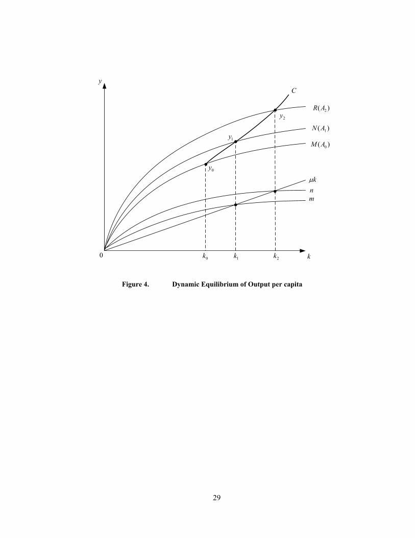
The dynamic equilibrium of per capita income for any type of economy can be determined in a simple way by representing these equations in a graph, as shown in Figure 4. In the initial period, given k0, A0 and δ0, and also given the growth rate of the labor supply (µ), the output per worker function is represented by the curve M; the investment function is represented by the curve m, and the line µk indicates the investment per worker needed to maintain the corresponding value of k constant. Given these initial conditions, therefore, the equilibrium level of output per capita is y0. This value determines investment per worker, the additional capital per worker, which lies above the value needed to maintain the capital-labor ratio constant at the initial level; the ratio k will then increase until it reaches the equilibrium value, which occurs at the point where the investment function cuts the line µk; hence equilibrium is reached at k1. In the following period, at the capital-labor ratio k1, technology changes to another level A1, which implies an upward shift of the output per worker function, from curve M to curve N; thus, the new equilibrium is y1. At this new level of technology, more investment is also induced and the investment function also shifts upward, to curve n; but, at k1, there is now more investment per worker than is needed to maintain k1 constant and this value will then increase. The new equilibrium will be k2. In the next period, at the value k2, the technology goes to level A2, which implies an upward shift in the curve of output per capita, from curve N to curve R, which in turn determines the new equilibrium value of output per worker y2, and so on. Hence, the dynamic equilibrium of output per worker shows a time path, which is given by the line C. According to this model, output per worker grows endogenously. The engine of growth is private investment because it induces the increase of both physical capital and technology, which is embodied in the new capital goods. These two effects lead to an increase of output, which in turn increases human capital. More human capital and a higher level of technology induce in turn to higher private investment, and so on. About the exogenous variables, two final assumptions are introduced now. First, the growth rate of labor supply will depend on the level of output per worker and thus becomes an endogenous variable. As the long run output per capita increases, population growth rates will fall. Therefore, in the long run the line µk in Figure 4 will shift downwards and the line C will become steeper over time. Second, the investment fund X will depend on the expectations of output growth, which in turn depend upon the observed growth rates of the economy; hence, this variable also becomes endogenous. Again, the consequence is to increase the slope of the line C over time. The line C in Figure 4 may refer to any of the three economies under study. However, their different initial conditions determine different time paths. Let the line C represent the time path of the epsilon economy. The sigma economy will, compared to epsilon, start at a lower value of k along the capital-labor axis; the initial value of y will also be lower due in part to the lower factor endowment, but also due to the low endowment of technology, which implies that y stands on a lower curve of output per worker. Omega economy’s initial conditions will lie in between. Investment per worker in sigma economy is equal or lower than in epsilon due to its relatively higher degree of inequality. The sigma-C line will thus fall below the epsilon-C line. No convergence will take place. Investment per worker in omega will be higher than in epsilon because these are socially homogeneous societies, in which inequality is less pronounced. The omega-C line will thus tend to converge towards the epsilon-C line.

20

New technologies are generated in epsilon, which implies that epsilon must generate these innovations in order to grow. In contrast, the technological gap that there exists between epsilon and sigma offers sigma a lot of room to grow and grow faster than epsilon because sigma only has to adopt new technologies already generated in epsilon. But this possibility is blocked by the low equality endowment of sigma. Omega takes advantage of the technological gap because it is a more equal society, in which social order is the norm. Among the three initial factors, capital stock (physical and human) can be accumulated and technology can be adopted endogenously; but the equality endowment cannot be accumulated endogenously. Private investment, the engine of growth, depends upon the degree of inequality of the society. The blocking factor in the process of economic growth in sigma society is, therefore, its very low equality endowment. The initial inequality is the ultimate factor in explaining the lack of convergence between sigma and epsilon economies. The unified dynamic model of economic growth of output per worker can then be represented as follows: y0 (t) = θ j ( k0 , A0 , δ0 ; t ), all θi>0, except θ3<0 (20)

where j=σ , ω, ε Given its initial conditions—factor endowments, technology endowments, and equality endowments—, each economy follows a particular time path. These inputs for the production of long run economic growth tend to converge endogenously between epsilon and omega, but it does not between epsilon and sigma. This equation shows that in the process of endogenous economic growth of capitalist economies, there exists path dependence; that is, history matters. What happens to income distribution in the process of endogenous capital accumulation? Although income inequality is an endogenous variable, capital accumulation does not change it significantly. The assumption of labor saving technological innovations implies that both profits and wage bill will rise with endogenous physical capital accumulation; hence, the change in the degree of income inequality in the capitalist sector is ambiguous. In the omega economy, the subsistence sector is residual, and changes in mean income, self-employment, and unemployment go in different directions. In the sigma economy, z-workers will be left behind, but overall inequality is still ambiguous. Finally, the accumulation of human capital is not equalizing either because the rich tend to accumulate more quantity of human capital than the poor. Z-workers are left behind in human capital accumulation because, being second rate citizens, they get low quality education and health as public goods. In sum, the long term degree of income inequality is determined by the initial inequality in the individual endowment of economic and social assets. The dynamic equilibrium of income inequality D can then be written as the consolidation of the relations obtained in the partial models, that is,

D0 (t) = G j ( δ0 ), G’ <0, where j=σ, ω, ε (21) A unified theory of distribution has then been reached. Inequality in the distribution of flows depends upon the initial inequality in the distribution of stocks. There may be short run variations, but in the long run the degree of income inequality depends on the

21

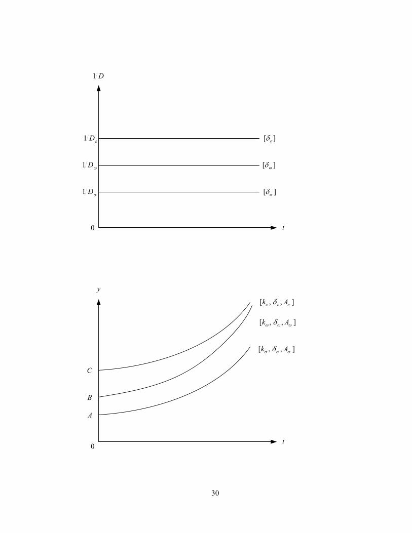
foundational shock of society; hence, there is path dependence in the inequality of capitalist economies. The unified theory of distribution—equation (21)—is represented in Figure 5. Panel (a) shows the time path of the degree of equality, namely 1/D. The curves are horizontal, indicating that the long run level of income inequality depends on the initial inequality. Because the epsilon society was “born” more equal than sigma society (that is, δε<δσ), the upper curve corresponds to epsilon society and the lower curve to sigma society. Epsilon societies were born relatively more equal and will continue to be so. Sigma societies were born relatively less equal and will continue to be so. The curve corresponding to the omega society will lie in between. In sum, the unified theory predicts no convergence in the degree of income equality. Regarding the unified theory of economic growth, shown in equation (20), it is graphically represented in Figure 5, panel (b). The time path of output per capita of each society is presented as rising curves. The top curve shows the case of the epsilon society and the bottom curve the case of the sigma society, while omega lies in between. These positions are the result of differences in the initial conditions of each society, which include factor endowments, technology endowments, and equality endowments. Sigma economy is poorly endowed with these growth inputs, while epsilon is highly endowed, and omega lies in between. The omega economy will approach the path of the epsilon economy because in the process of capital accumulation it will become an epsilon society. Omega and epsilon are socially homogeneous societies, with initial quantitative differences only. Sigma is a socially heterogeneous society and cannot become epsilon, unless it becomes omega first, which cannot occur endogenously. Sigma and epsilon are qualitatively and quantitatively different capitalist societies. The unified theory predicts convergence among some types of capitalist economies, but not an overall convergence. There may be short run changes in income levels in each economy caused by other exogenous variables, but they will vary around its long run curve, which is determined by its initial conditions. External shocks (like changes in the international terms of trade or the international interest rate) or domestic shocks (like disasters created by mother nature) generate economic cycles around the long run curve. Domestic monetary and fiscal policies can either reduce or amplify these cycles, which will certainly affect the supply of public goods. According to the theory presented here, investors have a long run view of society’s endowments of public goods—including here social order or political stability—and thus short run variations in the supply of public goods will not affect their behavior. Therefore, short run exogenous variables may have some effect on the long run economic growth, but they are not the essential factors. The interactions between short run fluctuations and the long run trajectories of output is an old unresolved question in standard economics. In his Nobel Price Lecture, Robert Solow stated, “The problem of combining long run and short run macroeconomics has still not been solved” (Solow 1988, p. 310). Indeed, for some economists, the short run fluctuations are just deviations from the long run growth path of output; for others, the long run trajectory is determined by the short run fluctuations, that is, short run fluctuations are not deviations from the long run growth path at all, but they constitute growth paths themselves. The theoretical approach developed here falls in the first position. Economic development defined as the mix of (y, 1/D) shows an endogenous trajectory that is determined by the initial conditions of society. Given the initial factor

22

endowments, the equality endowments, and the initial technological gaps, the trajectories of epsilon and sigma society will follow different time paths. VII. Conclusions The partial theories together with the unified theory developed in this study are able to explain the seven central empirical features of capitalism mentioned at the beginning of this study. The epsilon theory explains the particular features of the First World countries: the existence and persistence of unemployment, the interplay of nominal and real variables, the positive relation between real wages and real output in the long run. Omega and sigma theory seek to explain the Third World countries. The sigma theory explains the particular features of the Third World countries that have a significant colonial legacy: the existence and persistence of unemployment and underemployment, inequality between ethnic groups, the interplay between nominal and real variables, and the positive relation between real wages and real output in the long run. The omega theory is also able to explain these features in the Third World countries that do not have a strong colonial legacy. Hence, facts 1 to 5 are explained. The existence of good partial theories, however, does not guarantee a unified theory. Take the example of two good partial theories in physics: quantum mechanics and relativity, which are inconsistent with each other. This is not the case in this study, however. The unified theory is also able to explain the features of the capitalist economy as a whole. The unified theory predicts that omega economies will become epsilon economies endogenously, but sigma economies will not. Most Third World countries resemble sigma societies because they have significant colonial heritage, specially Latin American and Sub-Sahara African countries (Huntington 1997, Map 1.1). Hence, lack of convergence between the First World countries and the Third World countries is the rule, not the exception. Indeed, economic historian Angus Madison (1995) has shown that, since 1820, only Japan is the successful case of convergence, whereas South Korea and Taiwan will possibly join the First World group in the future. These cases of successful stories refer to socially homogeneous and low inequality countries, that is, omega type countries. In fact, the Gini coefficient of Japan (0.35), South Korea (0.34) and Taiwan (0.30) are very similar to the mean value (0.33) of the First World countries, but very apart from the mean values in Latin America (0.50) and Sub-Saharan Africa (0.45) (Deninger and Squire 1996, Tables 1 and 5). The unified theory developed here, therefore, predicts the existence and persistence of differences in income levels between the First World and the Third World countries. It also predicts the existence and persistence of differences in the degree of inequality between the First World and the Third World countries. Facts 6 and 7 are thus explained. In view of the consistency found between theory and reality, there is no reason to reject the unified theory at this stage of research. There are at least two groups of scholars in the literature that have recently studied the role of initial conditions in economic development. Economic historians constitute one group. They have shown the effect of European colonial systems on the economic development of different countries. They conclude that the initial institutions created at the foundational shock were in some cases utterly beneficial to investment and growth, but in other cases they were unfavorable, depending on the initial population density of

23

the colonies. Because most institutions are endogenous, the economic development of countries shows path dependence (Engerman and Sokoloff 2002; Acemoglu, Johnson, and Robinson 2002). The ultimate factor in explaining different paths of development is the initial factor endowment. The equality endowment plays no role. In the other group, the propositions come from biologists. They argue that Western superiority is based on geography, including the rich endowment of animals and plants (Diamond 1999). This is a complementary explanation to the unified theory. Several policy implications can be derived from this theoretical approach. Due to space limitations, just two points are mentioned here. First, the existence of different types of capitalist societies implies particular, not general, development prescriptions. Neoclassical growth theory refers to epsilon economies and cannot be applied to sigma economies. Robert Solow (2001) has indeed pointed it out: “I have never applied [neoclassical growth theory] to developing economies because I thought the underlying machinery would apply mostly to well-developed market economies” (p. 283). Second, the conclusion that history matters does not imply historical determinism. Economics is not like physics. What this conclusion means is that the policy prescriptions for less inequality within Third World countries and in the World Economy require the discovery of both the exogenous variables that can provide social actors the instruments to generate convergence and the particular social actors with the incentive compatibility to apply those measures. Breaking with history is certainly the main policy implication of the theoretical approach presented in this study. References Acemoglu, Daron, Simon Johnson, and James Robinson. 2002. “Reversal of Fortune: Geography and Institutions in the Making of the Modern World Income Distribution.” Quarterly Journal of Economics, 118, pp. 1231-1294. Akerlof, George and Rachel Kranton. 2000. “Economics and Identity.” Quarterly Journal of Economics, 115 (3), 715-733. Alesina, Alberto and Roberto Perotti. 1996. “Income Distribution, Political Instability, and Investment.” European Economic Review, 40: 1203-28. Barro, Robert and Xavier Sala-I-Martin. 1995. Economic Growth. McGraw Hill. Bowles, Samuel. 1985. “The Production Process in a Competitive Economy: Walrasian, Neo-Hobbesian, and Marxian Models.” The American Economic Review, 75 (1), March. Darity, William and Jessica Nembhard. 2000. “Racial and Ethnic Economic Inequality: The International Record.” The American Economic Review, 90, pp. 308-311. Deininger, Klaus and Lyn Squire. 1996. ‘A New Data Set Measuring Inequality’, The World Bank Economic Review, 10, pp. 569-591, September. Diamond, Jared. 1999. Guns, Germs, and Steel. The Fates of Human Societies. W.W. Norton.

24

Engerman, Stanley and Kenneth Sokoloff. 2002. “Factor Endowments, Inequality, and Paths of Development among New World Economies.” Economia, 3, pp. 41-109. Fogel, Robert. 1999. “Catching Up with the Economy.” American Economic Review, 89, pp. 1-21. Garraty, John. 1978. Unemployment in History. New York: Harper Colophon Books. Hall, Gillette and Harry Patrinos. 2005. Indigenous Peoples, Poverty, and Human Development in Latin America. London: Palgrave. Huntington, Samuel. 1997. The Clash of Civilizations and the Remaking of World Order. New York: Simon and Schuster Inc. ILO, International Labor Office. Annual. World Employment Report. Geneva. Li, Hongyi, Lyn Squire, and Heng-fu Zou. 1998. ‘Explaining International and Intertemporal Variations in Income Inequality’, Economic Journal, 108, 26-43, January. Maddison, Agnus. 1995. Monitoring the World Economy, 1820-1992. Paris: Development Center, OECD. Psacharopoulos, George and Harry Patrinos. 1994. Indigenous People and Poverty in Latin America. An Empirical Analysis. Aldershot. Rand, John and Finn Tarp. 2002. ‘Business Cycles in Developing Countries. Are they Different?’ World Development, 30, pp. 2071-2088. Sala-i-Martin, Xavier, Gernot Doppelhofer, and Ronald Miller. 2004. “Determinants of Long Term Growth: A Baysian Averaging of Classical Estimates (BACE) Approach.” American Economic Review, 94, pp. 813-35. Shapiro, Carl and Joseph Stiglitz. 1984. “Equilibrium Unemployment as a Workers Discipline Device.” The American Economic Review, 74 (3), June. Silva, Nelson. 2001. “Race, Poverty, and Exclusion in Brazil.” In E. Gacitua et al. (eds.), Social Exclusion and Poverty in Latin America and the Caribbean. Washington DC: The World Bank. Solow, Robert. 1998. “Growth Theory and After.” American Economic Review, 78, pp. 307-17. -----------. 2001. “Applying Growth Theory Across Countries.” The World Bank Economic Review, 15, pp. 283-88. Stewart, Frances. 2001. Horizontal Inequalities: A Neglected Dimension of Development. WIDER Annual Lectures, No. 5. Helsinki: United Nations University.

25

Wright, Erik. 1997. Class Counts. Comparative Studies in Class Analysis. Cambridge University Press.

26

Figure 1. Equilibrium in the Money and Labor Markets

.

e P

0 Dh

*h Q hS

H

' H

M

' M

F

E

G

•

• •

] S [ M m

] ' S [ ' M m

] z , K [ H ] ' z , ' K [ ' H

27

Workers

m’

ZBO

M

r’

Figure 2. General Equilibrium in Sigma Economy

m

w°

O’A

π w °

f'r *

m*E

g f

G R r

P°

W°

w vy vz

n

],,[ δAK

28

S0S1S 2S

1m

2m

][ 3ZC

M

0M F

][ 11 ZA

Figure 3. Investor’s Choice Between Economies with Different Endowments of Public Goods

3S

G

][ 22 ZA3m

29

)( 2AR

)( 1AN

)( 0AM

C

2y

1y

0y

0k 1k 2k

kµnm

k

y

0

Figure 4. Dynamic Equilibrium of Output per capita

30

][ εδ

][ σδ

D1

y

t0

0

],,[ εεε δ Ak

],,[ σσσ δ Ak

],,[ ωωω δ Ak

C

B

A

ωD1

σD1

εD1

t

][ ωδ