TOWARDS A UNIFIED DESCRIPTION OF KNOTTED

TOWARDS A UNIFIED DESCRIPTION OF KNOTTEDLIGHT

E. GOULART AND J. E. OTTONI

Abstract. Several complementary approaches to investigate knotted solu-tions of Maxwell’s equations in vacuum are now available in literature. How-ever, only partial results towards a unified description of them have beenachieved. This is potentially worrying, since new developments of the the-ory possibly lie at the intersection between the appropriate formalisms. Theaim of this paper is to pave the way for a theoretical framework in which thisunification becomes feasible, in principle.

1. Introduction

The theory of electromagnetic knots continues to spread new insights intothe behaviour of electromagnetism in nontrivial regimes (see [1] for a review).Roughly speaking, an electromagnetic knot is a solution of Maxwell’s equa-tions in vacuum whose field lines, at any given time, twist in 3-space formingknotted loops which may be pairwise linked. In the particular case of nullfields, the corresponding radiative solutions are called knotted light. Theseare characterized by nontrivial helicities and are adapted to an underlyinggeodesic, shear-free, null congruence, first discussed by I. Robinson [2, 3, 4].In [5], Irvine and Bouwmeester have shown how approximate knots of lightmay be generated using tightly focused circularly polarized laser beams,while recent numerical results were presented in [6]. Also, as discussed in[7], these solutions can be interpreted in terms of two codimension-2 space-time foliations, whose leaves intersect orthogonally everywhere in spacetime.

Since A. Rañada’s machinery based on a pair of time-evolving Hopf maps[8, 9, 10], several methods have been developed for constructing knotted nullfields. Among them the most proeminent are the following: A - Batemanconstruction, based on the introduction of constrained complex scalar fieldssatisfying a system of fully-nonlinear first order partial differential equations[11, 12]; B - Spinor/twistor method, in which twistor functions correspondto a class of torus knots and the Poynting vector structure forms the spatialpart of the Robinson congruence [13, 14]; C - Special conformal transforma-tions to generate new solutions from existing ones. This has enabled to geta wide class of solutions from the basic configurations like constant fields

1991 Mathematics Subject Classification. 78A25 (primary); 57R30, 57M25 (secondary).1

arX

iv:2

004.

0480

9v1

[m

ath-

ph]

9 A

pr 2

020

2 E. GOULART AND J. E. OTTONI

and plane-waves [15]; D - de Sitter method, based on a correspondence ofMaxwell solutions on Minkowski and de Sitter spaces, thanks to the con-formal equivalence between these spaces and the conformal invariance offour-dimensional gauge theory [16].

It has been pointed out that, since the known methods evolved largelyindependently, they also suggest different directions in which to expand thestudy of knotted light [1]. However, to the best of our knowledge, no system-atic approach to unify them in a rigorous theoretical framework exist in liter-ature. In order to shed some light on the debate, we think new ways to viewinterconnections between existing formalisms are very welcome. The aim ofthis paper is to discuss a framework where new interconnections emerge. Inparticular, using the machinery of quaternions, parallelizations and Maurer-Cartan forms, we show how the Bateman pairs and Rañada complex mapsare tied together. As a consequence, we show how to obtain several physicalquantities of relevance.

The paper is divided as follows: in section II we summarize null elec-tromagnetic fields and set concepts to be used throughout. In section IIIwe review the appropriate quaternionic machinery, introduce Lie frammings,Maurer-Cartan forms, adjoint maps and derive important relations. SectionIV presents some results in a complex representation, whereas section V usesthese results to establish a connection between Bateman pairs and Rañadacomplex maps. We conclude with some of possible developments that canbe explored.

2. Null electromagnetic fields

Let (M, g) denote Minkowski spacetime with signature convention (1, 3).The task of finding null solutions of the source-free Maxwell’s equations inan open set U ⊆M may be stated as follows. Find a nonzero complex 2-formR ∈ Ω2(U ,C) such that

(1) ? R = iR, R ∧R = 0, dR = 0,

with ? denoting the Hodge star operator with respect to g (?? = −1). Theself-duality condition guarantees that R = F − i ? F with F ∈ Ω2(U ,R):we identify F and ?F with the Faraday tensor and its dual. The secondcondition says that R is totally decomposable i.e., it splits as an exteriorproduct of complex 1-forms: this automatically defines a null field since thistop-degree identity is proportional to the invariants FabF ab and Fab ? F

ab.Finally, the closedness of R implies that F satisfies Maxwell’s equations invaccum. We shall call R a Riemann-Silberstein 2-form since the interiorproduct XyR, for a normalized timelike vector field X, is essentially E+ iB.

Let us briefly recall some known properties of Riemann-Silberstein 2-forms(see [17] for a detailed discussion). Due to purely algebraic considerations,

KNOTTED LIGHT 3

they split as an exterior product

(2) R = k[ ∧m[

where k and m are mutually orthogonal null vectors (with k real) and k[,m[ the canonical contractions with the metric via musical isomorphisms.Formally, the principal null field k is a section of the null cone bundle Nover U , the closedness of R implying that the flow generated by k constitutea shear-free null geodesic congruence: we say that the electromagnetic fieldis adapted to k. Now, at a given spacetime point x, the set k⊥x = v ∈TxM |g(k, v) = 0 defines a 3-dimensional vector space containing k and,associated to k⊥x there is a two-parameter family of real spacelike planes, thescreen spaces of k. The set of all screens at all spacetime points constitute abundle k⊥/k, called the umbral bundle. It is clear that if k(x) and m(x) aresections of N and k⊥/k, respectively, the self-duality of R is then related toa rotation by 900 of the screen onto itself i.e., ?R = k[ ∧ im[.

An additional property of Riemann-Silberstein 2-forms is that they in-duce two codimension-2 foliations of Minkowski spacetime (F1 and F2). Thecorresponding involutive distributions are given by

(3) ∆1 = ker Re(R) ∆2 = ker Im(R)

and the integral manifolds are 2-dimensional embedded surfaces ruled by nullgeodesics. The family of all such surfaces constitute a particular instance ofthe (2, 2) dual foliations defined in [7]. Following this reference, we shall callthe leaves of F1 and F2, magnetic and electric, respectively.

The case of knotted light we discuss here, the Hopf-Rañada solution, is abeautiful realization of a (2, 2) dual foliation. For this solution, the electro-magnetic field is adapted to a twisting congruence of light rays (the Robinsoncongruence) and the magnetic/electric leaves are pairwise linked once. Fur-thermore, if u is tangent to a magnetic leaf and v is tangent to an electricleaf, then g(u, v) = 0. We shall see that the anatomy of this solution isintimately related to the internal structure of quaternions, which permits adirect route from the formalism of Bateman pairs to RaÃśadaâĂŹs complexmappings. Furthermore, our approach reinforces aspects of knotted lightwhich are similar in spirit to some aspects of mathematical gauge theory(specially on the construction of instantons).

3. Quaternionic machinery

3.1. Invariant vector fields and Lie framings. To begin with, we iden-tify the four-dimensional Euclidean space (R4, δ) with the associative alge-bra of real quaternions H by giving Hamilton’s multiplication table for thecanonical basis e0, ..., e3

(4) e0eµ = eµe0 = eµ, eiej = −δije0 + ε kij ek.


A typical quaternion and its conjugate then take the form1

(5) q = qµeµ = q0e0 + qiei q = qµeµ = q0e0 − qiei

and there follow pq = qp. As usual, the real part of a quaternion is identifiedwith Re0 whereas the imaginary part is identified with the vector quantityRe1 + Re2 + Re3. The norm of a quaternion || || : H → R≥0 is defined by||q|| =

√qq whereas the inverse reads as q−1 = q/||q||2. In what follows, H∗

denotes the Lie group of non-zero real quaternions while the unit three-sphereS3 is interpreted as the compact subgroup

Sp(1) = u ∈ H∗| ||u|| = 1.

Since a generic quaternion may be written as q = ||q||u with u ∈ S3, one seesthat H∗ = R+ × Sp(1). Hence, H∗ is foliated by the level sets of ||q||, whichare nothing but real three-spheres centered at the origin.

Now, as H∗ is parallelizable, the left and right translations lq, rq : H∗ →H∗ permit the construction of two globally defined Lie framings: the leftinvariant framing ϕ− = L0, ..., L3 and the right invariant framing ϕ+ =R0, ..., R3. Specifically, we take

(6) Lα(q) = qeα Rα(q) = eαq

and a direct calculation yields the vector fields

L1 = (−q1, q0, q3,−q2) L2 = (−q2,−q3, q0, q1) L3 = (−q3, q2,−q1, q0)R1 = (−q1, q0,−q3, q2) R2 = (−q2, q3, q0,−q1) R3 = (−q3,−q2, q1, q0)

with L0 = R0 = (q0, q1, q2, q3). It is easily checked that these fields satisfythe algebraic relations

(7) Lα · Lβ = ||q||2δαβ Rα ·Rβ = ||q||2δαβ

where · is the Euclidean scalar product in (R4, δ) and that the Lie bracketsread as

(8) [Lα, Lβ] = c γαβ Lγ , [Rα, Rβ] = −c γ

αβ Rγ , [Rα, Lβ] = 0,

with structure constants given by c kij = 2εijk and all others equal to zero.

Consequently, one concludes that the radial field commutes with all otherfields and that the framings ϕ± automatically induce two complementaryparallelizations ϕ±|Sp(1), when restricted to the unit 3-sphere. The latter

are independent cross-sections of the bundle of orthonormal frames O(S3).

1Throughout, lower-case Greeks run from 0 to 3 and lower-case Latins run from 1 to 3.

KNOTTED LIGHT 5

3.2. Maurer-Cartan forms, co-frames and rank-2 foliations. In orderto deepen on the structure of the invariant vector fields it is illuminatingto work within the dual picture. Since left and right invariant fields leadbasically to the same theory, we shall concentrate our analysis on the leftinvariant case. To do so, we define the left invariant Maurer-Cartan one-form

(9) λ ≡ q−1dq = λµ ⊗ eµ

which satisfy, by construction, the relations 〈λ, Lα〉 = eα. Morally we canthink of the Maurer-Cartan form as a compact way to write the standardleft-parallelization of the tangent bundle of H∗. Direct calculation, usingEqs. (9), give

(10) λ = d(ln||q||)⊗ e0 + ||q||−2(q0dqi − qidq0 − εi jkqjdqk)⊗ ei,

and writting the quaternion as q = ||q||u, there follow

(11) λ = d(ln||q||)⊗ e0 + (u0dui − uidu0 − εi jkujduk)⊗ ei

which implies in

(12) Re(λ) = d(ln||q||), Im(λ) = udu.

From now on, we shall stick to Eq. (11) instead of Eq. (10) since it leads tosimpler expressions.

Using the identity

(13) du = −uduu

one shows that λ satisfies the Maurer-Cartan structure equations [18, 19]

(14) dλ = d Im(λ) = −Im(λ) ∧ Im(λ) = −1

2[Im(λ) ∧ Im(λ)].

We then read off the relations

(15) dλ0 = 0, dλi = −(εi jkλj ∧ λk),

implying that each non-vanishing component of the differential is a totallydecomposable (simple) 2-form. Notice that although the Maurer-Cartanform itself is H-valued their exterior derivatives take values in Im(H) ∼=sp(1)L. Explicit calculation, using Eq. (11), gives

dλ = (2du0 ∧ dui − εi jkduj ∧ duk)⊗ ei.(16)

An interesting property of dλ is that it induces three left-invariant codimension-2 foliations on H∗. Indeed, as a consequence of Eq. (15), we have:

(17) dλ = −2(λ2 ∧ λ3 ⊗ e1 + λ3 ∧ λ1 ⊗ e2 + λ1 ∧ λ2 ⊗ e3).


Defining the rank-2 distributions

Di ≡ ker(dλi) = kerλj ∩ kerλk = span(L0, Li)(18)

with i 6= j 6= k, one may easily check that the latter are integrable inthe sense of Frobenius [20, 21]. This means that each 2-plane field defineintegral manifolds. The associated foliations F i are transversal to Sp(1) and,therefore, one may interpret the integral curves of the invariant vector fieldLi (restricted to Sp(1)) as intersections of the corresponding foliation withthe latter.

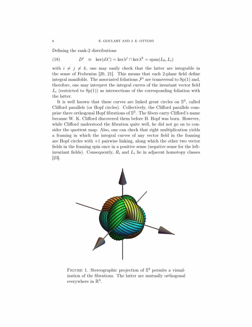
It is well known that these curves are linked great circles on S3, calledClifford parallels (or Hopf circles). Collectively, the Clifford parallels com-prise three orthogonal Hopf fibrations of S3. The fibers carry Clifford’s namebecause W. K. Clifford discovered them before H. Hopf was born. However,while Clifford understood the fibration quite well, he did not go on to con-sider the quotient map. Also, one can check that right multiplication yieldsa framing in which the integral curves of any vector field in the framingare Hopf circles with +1 pairwise linking, along which the other two vectorfields in the framing spin once in a positive sense (negative sense for the left-invariant fields). Consequently, Ri and Li lie in adjacent homotopy classes[23].

Figure 1. Stereographic projection of S3 permits a visual-ization of the fibrations. The latter are mutually orthogonaleverywhere in R3.

KNOTTED LIGHT 7

3.3. The adjoint map and leaf description. In order to describe the2-dimensional leaves of F i explicitly, we start by recalling that H∗ acts onitself via the adjoint map

(19) ad : H∗ ×H∗ → H∗, ad(q, q′) = qq′q−1 = uq′u.

Clearly, this action leaves Im(H) as an invariant subspace and if q′ belongsto the equator of Sp(1) i.e., the intersection of the 3-plane spanned by theunits ei with the unit three-sphere, ad(q, q′) automatically induces a mapfrom H∗ to S2 ⊆ Sp(1). Specifically, we consider the quaternionic maps

(20) lj(q) = uej u = eiQi j(q)

where

(21) Qi j =

(u20 − ukuk)δi j + 2uiuj − 2u0εijku

k

with uµ = δµνuν . In matrix notation, one obtains

(22) Q =

u20 + u21 − u22 − u23 2(u1u2 − u0u3) 2(u1u3 + u0u2)2(u1u2 + u0u3) u20 − u21 + u22 − u23 2(u2u3 − u0u1)2(u1u3 − u0u2) 2(u2u3 + u0u1) u20 − u21 − u22 + u23

.

By direct calculation one shows that QTQ = 1 and det(Q) = 1, henceQ ∈ SO(3). It is easy to show that the integral manifolds associated tothe distributions Di are given by the inverse images of the li. Indeed, thedifferential maps

(23) dli : TqH∗ → Tad(q,ei)S2

are given as follows

dli = dueiu+ ueidu = u[λ, ei]u = 2λj ⊗ ε kji lk(24)

and one obtains

〈dli, Lm〉 = 2ε kmi lk → L0, Li ∈ ker(dli)(25)

which proves the assertion.A remarkable property of the Maurer-Cartan forms λi is that their dif-

ferentials descend to S2. The claim is that there is a normalized 2-form Ω2

on S2 whose pullbacks along the maps described above define the exteriorderivatives dλi. Start with the normalized volume form on S2 given by

(26) Ω2 =1

8πn · (dn ∧ dn) =

1

8πεijkn

idnj ∧ dnk


with n = niei ∈ Im(H) and ||n|| = 1. The pullback of Ω2 along the maps liread as (no summation)

l∗iΩ2 =1

8πli · (dli ∧ dli)(27)

Using Eq. (24), we get

l∗iΩ2 =1

2πλp ∧ λq ⊗ ε k

ip ε liq li · (lkll)

=1


ip ε liq li · (uekelu)

=1


ip ε liq ε

mkl δim

=1

2πεipqλ

p ∧ λq

where we have used the fact that li · lj = δij . From these relations we getthe alternative representation of the differentials

(28) dλi = −2πl∗iΩ2.

With this expression, the calculus of the Hopf invariants associated to theleft-invariant vector fields Li restricted to S3 are straightforward. Indeed,restricting the three maps li to S3 it is easily seen that they define threeproper submersions and we have, by definition:

(29) H(li) =

∫S3ωi ∧ dωi (no summation)

with dωi = l∗iΩ2. Using (28) and noticing that Ω3 = λ1 ∧ λ2 ∧ λ3 is theinvariant volume form on S3, we get H(li) = −1. We shall see in Section Vthat Eqs. (28) together with Eqs. (15) form the basic clue for connecting theformalism of Bateman’s pairs with Rañada’s complex mappings approach.In order to do this we first describe some relevant quantities in complex form.

4. Complex representation

AlthoughH is not properly a complex algebra, nonethless, for our purposesit is convenient to represent H as a real algebra over C2 (see [22]). In orderto do this we revert to the classical notation 1, i, j, k for the principalunits and consider the decomposition H = C⊕ jC. A typical quaternion, itsconjugate and the Hermitian scalar product then take the form

(30) q = z1 + jz2 q = z1 − jz2 ||q||2 = z1z1 + z2z2

in which we have introduced the complex coordinates z1 = q0 + iq1 andz2 = q2 − iq3. Since several previous expressions are simpler when writtenin terms of unit quaternions, we write u = v1 + jv2 and (9) becomes

λ = d(ln||q||) + (v1dv1 + v2dv2) + j(v1dv2 − v2dv1),(31)

KNOTTED LIGHT 9

whereas its exterior derivative is given by

dλ = (dv1 ∧ dv1 + dv2 ∧ dv2) + j2(dv1 ∧ dv2).(32)

Writting the matrix Q in Eq. (22) in terms of the complex components,we obtain the quaternionic maps:

l1 = (v1v1 − v2v2)i+ j2iv1v2

l2 = (v1v2 − v1v2) + j(v21 + v22)

l3 = (v1v2 + v1v2)i+ ji(v22 − v21)

It is convenient for our purposes, however, to perform a stereographic pro-jection

(33) σ : S2 \ (−1, 0, 0)→ CP1 \∞ ∼= C

onto the second copy of C. In order to obtain the most appealing geometricalresults we use

(34) n 7→ ζ =n2 − in3

1 + n1

and there follow the composite maps ζi : H∗ → C

ζ1 = iv2v1

ζ2 =(v1 + iv2)

(v1 + iv2)ζ3 = i

(v2 − v1)(v2 + v1)

(35)

where ζi = σli. Therefore, in order to describe explicitly one of the foliationsdefined by Eqs. (18), simply take the appropriate map and consider itspreimages. Clearly, each leaf is a complex line through the origin in H∗.Interestingly, since the normalized volume form on S2 may be written asΩ2 = 1

2πidζ ∧dζ/(1 + ζζ)2 one must have, as a consequence of Eqs. (28) and(35) the identities (no summation)

(36) dλj = idζj ∧ dζj

(1 + ζj ζj)2

5. Connection of Bateman pairs and Rañada complex maps

In order to reproduce the Hopf-Rañada solution using the co-framings de-scribed so far we proceed very much in the same way as gauge theorists.To begin with, we let P (M, Sp(1)) denote the principal Sp(1) bundle overMinkowski spacetime M and consider a section s : M → P (M, Sp(1)), de-fined by

(37) u(t, x) = α(t, x) + jβ(t, x),


with α, β ∈ F(M,C) and |α|2 + |β|2 = 1. As usual, we require that points atspatial infinity inM are mapped to the same point in Sp(1), for all times. Tobe specific, we assume u(t,∞) = e0, which effectively compactifies spacetimeto the product manifold R × S3, and s can be thought of as some sort of‘gauge function’. The pullback of the Maurer-Cartan form along s defines asp(1)L-valued one-form in spacetime

(38) s∗λ = (αdα+ βdβ) + j(αdβ − βdα).

Notice that the first term in the r.h.s is purely imaginary since αα+ββ = 1.The exterior derivative is

(39) d(s∗λ) = (dα ∧ dα+ dβ ∧ dβ) + 2j(dα ∧ dβ).

Now, suppose that we manage to find a smooth section satisfying the fullynonlinear system of first order partial differential equations

(40) ? (dα ∧ dβ) = i(dα ∧ dβ) 6= 0.

Connection with the electromagnetic field comes with the identification

(41) R = 2dα ∧ dβ,

where (α, β) plays the role of Bateman pairs and the Faraday tensor is given,as before, by the real part of R. Since the complex 2-form R qualifies as aRiemann-Silberstein 2-form it may be written asR = k[∧m[ and one obtains,after simple manipulations:

k[ = −i(αdα+ βdβ),(42)m[ = 2i(αdβ − βdα).(43)

It can be checked that these quantities satisfy

(44) g(k, k) = 0 g(m,m) = 0 g(k,m) = 0

as expected. Consequently, one sees that k(x) and m(x) are necessarilysections of N and k⊥/k, respectively. Due to Robinson theorem [4], k isgeodesic and shear free.

With the above conventions, there follow also the useful relations

(45) dk[ ∧ k[ 6= 0, dk[ = im[ ∧ m[/4, dm[ = 2ik[ ∧m[

from which one concludes that k is a rotating congruence and R = d(m[/2i).Therefore, the formalism provides a set of internal relations which reveals arich mathematical structure, connecting at once several quantities of physicalrelevance. In order to further explore such connections one uses the diagram

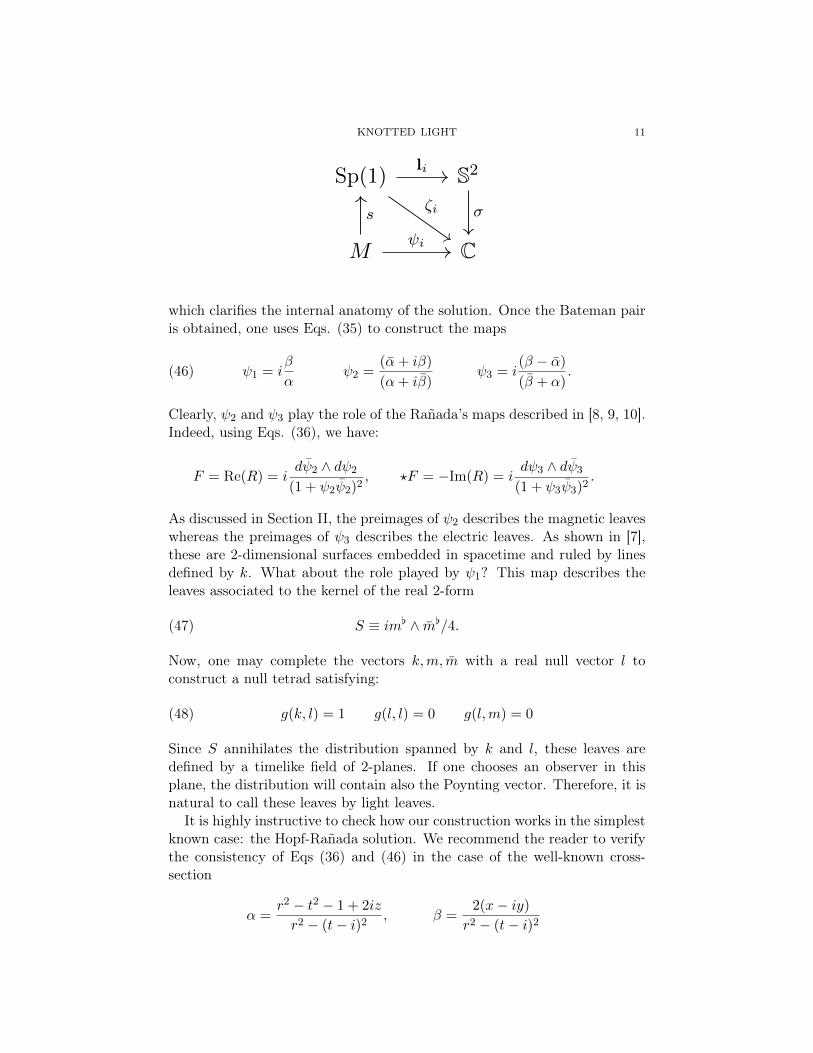
KNOTTED LIGHT 11

Sp(1) S2

M C

li

ζi σ

ψi

s

which clarifies the internal anatomy of the solution. Once the Bateman pairis obtained, one uses Eqs. (35) to construct the maps

(46) ψ1 = iβ

αψ2 =

(α+ iβ)

(α+ iβ)ψ3 = i

(β − α)

(β + α).

Clearly, ψ2 and ψ3 play the role of the Rañada’s maps described in [8, 9, 10].Indeed, using Eqs. (36), we have:

F = Re(R) = idψ2 ∧ dψ2

(1 + ψ2ψ2)2, ?F = −Im(R) = i

dψ3 ∧ dψ3

(1 + ψ3ψ3)2.

As discussed in Section II, the preimages of ψ2 describes the magnetic leaveswhereas the preimages of ψ3 describes the electric leaves. As shown in [7],these are 2-dimensional surfaces embedded in spacetime and ruled by linesdefined by k. What about the role played by ψ1? This map describes theleaves associated to the kernel of the real 2-form

(47) S ≡ im[ ∧ m[/4.

Now, one may complete the vectors k,m, m with a real null vector l toconstruct a null tetrad satisfying:

(48) g(k, l) = 1 g(l, l) = 0 g(l,m) = 0

Since S annihilates the distribution spanned by k and l, these leaves aredefined by a timelike field of 2-planes. If one chooses an observer in thisplane, the distribution will contain also the Poynting vector. Therefore, it isnatural to call these leaves by light leaves.

It is highly instructive to check how our construction works in the simplestknown case: the Hopf-Rañada solution. We recommend the reader to verifythe consistency of Eqs (36) and (46) in the case of the well-known cross-section

α =r2 − t2 − 1 + 2iz

r2 − (t− i)2, β =

2(x− iy)

r2 − (t− i)2


with r2 = x2 + y2 + z2. For this solution the Riemann-Silberstein 2-formread as

R = 8iC−3[(x− iy)2 − (t− z − i)2]ω1 + i[(x− iy)2 + (t− z − i)2]ω2

−2[(x− iy)(t− z − i)]ω3

with

C = r2 − (t− i)2

ω1 = dt ∧ dx+ idy ∧ dzω2 = dt ∧ dy + idz ∧ dxω3 = dt ∧ dz + idx ∧ dy,

and, using Eqs. (42) and (43), the Robinson congruence (k) and the screens(m) emerge naturally, if we raise indices with the contravariant metric.

6. Conclusion

Knotted and linked fields have been investigated in a variety of physicalsystems: hadron models, topological MHD, classical/quantum field theories,DNA topology, nematic liquid crystals, fault resistant quantum computingamong others. In this paper we propose a framework in which a unifieddescription of knotted light becomes transparent.

Since it is well known how to translate the spinor/twistor formalism intoBateman pairs [13], we have focused our attention on interconnections be-tween the latter and Rañada’s complex maps. Starting with a general de-scription of null fields in terms of Riemman-Silberstein 2-forms, we discusssome bundles of physical interest and review some results concerning folia-tions presented in [7]. We then move to the notion of a parallelization onH∗ and derive several useful relations using the Maurer-Cartan forms andthe corresponding structure equations. The latter is an essential ingredientin showing that the differential of the Maurer-Cartan form may be obtainedfrom maps to the 2-sphere. We show the explicit form of these maps anddiscuss how their preimages define three codimension-2 foliations of H∗. In-tersections of the corresponding complex curves with the 3-sphere give riseto three orthogonal Hopf fibrations. In order to reproduce the Hopf-Rañadasolution in terms of the co-frames thus described we proceed very muchin the same way as gauge theorists. We consider a principal Sp(1) bundleover spacetime and consider a section satisfying a system of fully nonlin-ear PDE’s. These equations automatically translates into Bateman pairs.The underlying formalism then give, with simple manipulations: the cor-responding Rañada’s complex maps plus a map whose preimages describethe 2-diemansional leaves associated to the Poynting vector, the Robinsoncongruence, the section of the umbral bundle and all related potentials.

KNOTTED LIGHT 13

We hope that the construction presented here may shed some light in fur-ther developments of the theory. In particular, it should be interesting toinvestigate whether the holomorphic approach h : H→ H, which give rise tonew Bateman pairs, fits in the scenario discussed in the paper. This couldgive a definitive proof if there exist topology preserving solutions derivedfrom Seifert fibrations. We shall investigate these questions in a forthcom-ming paper.

References

[1] M. Arrayás, D. Bouwmeester and J.L. Trueba. “Knots in electromagnetism”; PhysicsReports Vol 667 1-62 (2017).

[2] J. L. Trueba and A. F. RaÃśada. “The electromagnetic helicity”; European Journalof Physics, no.17.3 141 (1996)

[3] M. Elbistan, C. Duval, P. A. Horvathy and P.M. Zhang. “Duality and helicity: asymplectic viewpoint”; Physics Letters B, no. 761, 265-268 (2016)

[4] I Robinson. “Null electromagnetic fields”; J. Math. Phys. Vol 2 No. 3 290-291, (1961).

[5] Irvine, William TM, and Dirk Bouwmeester. “Linked and knotted beams of light”;Nature Physics 4.9 (2008): 716-720.

[6] Valverde, Antonio M., et al. “Numerical simulation of knotted solutions for Maxwellequations”; arXiv preprint arXiv:2003.01896 (2020).

[7] e Silva, W. Costa, E. Goulart, and J. E. Ottoni. “On spacetime foliations and electro-magnetic knots”; Journal of Physics A: Mathematical and Theoretical 52.26: 265203.(2019).

[8] A.R. Rañada. “A topological theory of the electromagnetic field”; Lett. Math. Phys.Vol 18 97 (1989).

[9] A.R. Rañada. “Knotted solutions of the Maxwell equations in vacuum”; Journal ofPhysics A: Mathematical and General 23.16 (1990): L815.

[10] A.R. Rañada. “Topological electromagnetism”; Journal of Physics A: Mathematicaland General 25.6 (1992): 1621.

[11] H. Bateman. “The Mathematical Analysis of Electrical and Optical Wave-Motion onthe Basis of MaxwellâĂŹs Equations”; (Dover, 1955).

[12] Besieris, Ioannis M., and Amr M. Shaarawi. “Hopf-RanÃčda linked and knotted lightbeam solution viewed as a null electromagnetic field”; Optics letters 34.24 (2009):3887-3889.

[13] Kedia, Hridesh and Bialynicki-Birula, Iwo and Peralta-Salas, Daniel and Irvine,William T. M. “Tying Knots in Light Fields”; Phys. Rev. Lett., 111.15, 150404 (2013).

[14] R. Penrose. “Twistor Algebra”; Journal of Mathematical Physics 8:2, 345-366 (1967).

[15] C. Hoyos, N. Sircar, J. Sonnenschein. “New knotted solutions of Maxwell’s equations”;Journal of Physics A: Mathematical and Theoretical 48 (2015) 255204 .

[16] O. Lechtenfeld and G. Zhilin. “Rational Maxwell knots via de Sitter space”; Journalof Physics: Conference Series 1194, 012068 (2019).

[17] Holland, Jonathan, and George Sparling. “Null electromagnetic fields and relativeCauchyâĂŞRiemann embeddings”; Proceedings of the Royal Society A: Mathematical,Physical and Engineering Sciences 469.2152 (2013): 20120583.

[18] Nakahara, M. “Geometry, topology and physics”; CRC Press, (2003).

http://arxiv.org/abs/2003.01896


[19] Isham, Chris J. “Modern differential geometry for physicists”; Vol. 61. World Scientific,(1999).

[20] J. M. Lee. “Introduction to smooth manifolds”; Springer, 2013.

[21] R. M. Wald. “General relativity”; University of Chicago press, (2010).

[22] Delphenich, David H. “The representation of physical motions by various types ofquaternions”; arXiv preprint arXiv:1205.4440 (2012).

[23] Wilson, F. Wesley. “Some examples of vector fields on the 3-sphere”; Annales del’institut Fourier, tome 20, n.2 (1970), p.1-20.

Departamento de Física e Matemática CAP-Universidade Federal de SãoJoão del-Rei, Rod. MG 443, KM 7, 36420-000, Ouro Branco, MG, Brazil

E-mail address: [email protected]

Departamento de Física e Matemática CAP-Universidade Federal de SãoJoão del-Rei, Rod. MG 443, KM 7, 36420-000, Ouro Branco, MG, Brazil

E-mail address: [email protected]

http://arxiv.org/abs/1205.4440

Documents

TOWARDS A UNIFIED DESCRIPTION OF KNOTTED