Embed Size (px)
Citation preview
Toward Understanding the Quark Parton Model of Feynman
W-Y P Hwang
Department of Physics National Taiwan University
Taipei Taiwan 10764 ROC
Invited paper presented at the 199pound Physical Society of Republic of China
January pound4 - pound5 199pound Taipei Taiwan R O C
Toward Understanding the Quark Parton Model of Feynman
W-Y P Hwang
Department of Physics National Taiwan University
Taipei Taiwan 10764 ROC
Abstract
The quark parton model of Feynman which has been used for analyses of
high energy physics experiments invokes a set of parton distributions in the
description of the nucleon structure (the probability concept) contrary to the
traditional use of wave functions in nuclear and medium energy physics for
structural studies (the amplitude concept) In this paper I first review briefly
how the various parton distributions of a nucleon may be extracted from high
energy physics experiments I then proceed to consider how the sea distribushy
tions of a free nuc~eon at low and moderate Q2 (eg up to 20GeV2) may
be obtained in the meson-baryon picture a proposal made by Hwang Speth
and Brown Using the form factors associated with the couplings of mesons to
baryons such as 7rNN 7rN6 and KNA couplings which are constrained by
the CCFR neutrino data we find that the model yields predictions consistent
with the CDHS and Fermilab E615 data on the sea-to-valence ratio We also
find that the recent finding by the New Muon Collaboration (NMC) on the
violation of the Gottfried sum rule can be understood quantitatively Finally
we consider using the pion as the example how valence quark distributions of
a hadron may be linked to the hadron wave function written in the light-cone
language Specifically we use the leading pion wave function that is constrained
by the QeD sum rules and find that at Q2 ~ (05 GeV)2 the leading Fock
component accounts for about 40 of the observed valence quark distributions
in the pion The question of how to generate the entire Valence quark distrishy
butions from the valence quark distribution calculated from the leading Fock
component is briefly considered again using the specific proposal of Hwang
Speth and Brown
Invited paper pre8ented at the 1992 PhY8icai Society of Republic of China
January 24 - 25 1992 Taipei Taiwan R O C
1
I IntrodDetion
The physics Nobel prize in 1990 was awarded to Jerome Friedman Henry
Kendall and Richard Taylor for the celebrated SLAC-MIT experiments) which
were carried out in late 1960s The experiments demonstrate that at large
Q2 with Q2 the four-momentum transfer squared or equivalently at very high
resolution (typically in the sub-fermi range) a nucleon (proton or neutron)
looks like a collection of (almost non-interacting) pointlike partons Nowadays
we identify these partons as quarks antiquarks and gluons Consequently a
nucleon is described by a set of structure functions or distributions
u(xQ2) u(xQ2) d(xQ2) d(xQ2) s(xQ2) S(XQ2) (1)
g(x Q2)
Here x is the fraction of the hadron longitudinal momentum carried by the
parton as visualized2 in the infinite momentum frame (Pz -+ 00)
High energy physics experiments with hadrons including deep inelastic scatshy
tering (DIS) by charge leptons (e or 1-) Drell-Yan (DY) production in hadronic
collisions (A+B -+e+ +l-+X) experiments with high energy neutrino beams
charm production with high energy neutrinos and others all have customarily
been analyzed in the framework of the quark parton model as proposed by R
P Feynman2
On a different front the idea of quarks or antiquarks as the buliding blocks
of hadrons was proposed3 in 1964 by Gell-Mann and independently Zweig
Since then quark models in a variety of detailed forms have been introduced
and shown to describe quite successfully the structure of hadrons For instance
a proton (or neutron) at low Q2 may be treated approximately as a system of
three quarks (u u d) (or (d d u)) confined to within a region defined by the
hadron size (perhaps with each of the quarks dressed by quark-anti quark pairs
2
or gluons) Unlike what is in the parton model where one adopts distributions
to describe a nucleon (at large Q2) one uses wave functions in the quark model
to characterize the structure of a nucleon (at low Q2) The dual picture for
describing the nucleon structure has generated the impression that the inforshy
mation acquired from high energy physics experiments seems to some extent
irrelevant for low energy strong interaction physics which are described very well
by the meson-baryon picture via wave functions (rather than via distributions)
Nowadays it is believed that quantum chromodynamics (QCD)4 describes
strong interactions among quarks and gluons The existence of quarks or
antiquarks is beyond doubt even though a quark or antiquark in isolation is not
found experimentally The experimental information points to the confinement
of color - namely quarks antiquarks and gluons all carry colors and only colorshy
singlet or colorless objects may be found in the true ground state (vacuum)
of QCD Accordingly quarks antiquarks and gluons must organize themselves
into colorless clusters (hadrons) in the true vacuum leading to the observation
that low energy strong interaction physics (or hadron physics) can successfully
be described effectively in terms of mesons and baryons (the meson-baryon
picture )
Although the gap between high energy (particle) physics and nuclear physics
is quite understandable owing to the dual picture for describing the nucleon
structure at large Q2 and small Q2 we nevertheless believe that such gap is
caused primarily by our ignorance toward the physics associated with the quark
parton model of Feynman2 Should it become possible to obtain quantitatively
the various parton distributions from a quark model (perhaps augmented with
the meson-baryon picture) the information extracted from particle physics exshy
periments is then complementary rather than orthogonal (as of today) to that
3
deduced from low energy strong interaction physics It is the purpose of the
present paper to provide an overview of recent efforts mostly of our own as
much more space and time would be needed for a truly comprehensive review
in trying to understand the quark parton model of Feynman2
4
II Parton Distributions as Inferred from Experiments
To unravel the structure functions of a nucleon it is customary to employ
deep inelastic scatterings (DIS) of the various kind including (a) DIS by charge
leptons (b) experiments with high energy neutrino beams (c) heavy flavor
production by high energy neutrinos and others In addition Drell-Yan (DY)
lepton pair production in hadronic collisions has also yielded indispensible inshy
formation concerning parton distributions associated with a hadron In what
follows we illustrate briefly these reactions in connection with parton distribushy
tions of a proton
(a) Deep Inela8tic Scattering8 by Charge Lepton8
Consider the DIS by electrons or muons
l(l) +p(P) ~ l(pound) + X (2)
We may adopt the following kinematic variables
(3a)
(3b)
(3c)
(3d)
(3e)
Here the metric is chosen to be pseudo-Euclidean such that q2 == q2 - Q5 but
we shall use wherever possible the variables Q2 v x y and others which are
5
metric-independent and are adopted fairly universally in the literature Note
that in Eqs (3a) (3b) and (3d) the last equality holds only in the laboratory
frame The differential cross section for the DIS process Eq (2) may be cast
in any of the following forms
tPu 2 tPu dxdy = v(s - mN) dQ2dv
2) tPu( (4)=xs-mN dQ2dx
21rmNV ~u - Ell dOldEl
In particular we have
~u 21rQ 2 2 ( 2)
-dd =--r2 l+(l-y) F2 xQ (5a)x y sx y
with
(5b)
Here the summation over the flavor index i extends over all quarks and anti-
quarks (See Eq (1)) Thus DIS with a proton target allows for the measureshy
ment of the structure function FP(x Q2)
FP(x Q2) = ~x(uP(x Q2) + uP(x Q2)) + ~x(dP(x Q2) + dP(x Q2)) (6)
1+ gX(sP(x Q2) + sP(x Q2)) +
On the other hand DIS with a neutron target (often with a deuteron target
with the contributions from the proton suitably subtracted) yields
Fn(x Q2) = ~xW(x Q2) + iln(x Q2)) + ~x(un(x Q2) + un(x Q2)) (7)
1+ gx(sn(x Q2) + sn(x Q2)) +
The proton and neutron are two members of an isospin doublet Assuming
isospin symmetry we haye dn(x) = uP(x) dn(x) = uP(x) un(x) = dP(x)
6
sn(x) =sP(x) etc Eq (7) becomes
rn(X Q2) 0 ~x(uP(x Q2) + fiP(x Q2)) + ~x(dl(x Q2) + iIP(x Q2)) (8)
+ ~x(sP(x Q2) + sP(x Q2)) +
Taking the sum of Eqs (6) and (8) we find
[ FP(x Q2) + Fn(x Q2)dx
5 (9)=glt x gtu + lt X gtu + lt X gtd + lt x gtl + lt x gt + lt x gt + 1
- 3lt xgt + lt x gt +
where lt x gti== fa i(X Q2)dx is the total momentum fraction carried by the
quarks (antiquarks) of flavor i Using the deuteron as the target and neglecting
the very small correction from heavy quarks we conclude from the SLAC-MIT
experiments that in the proton the total momenta carried by all quarks and
antiquarks add up to only about (40 - 50) of the proton momentum leaving
the rest of the momentum for electrically neutral partons (such as gluons)
On the other hand we may take the difference between Eqs (6) and (8)
and obtain
SG == 11
dx FP(x) _ Fn(x) o x
= ~ [1 uP(x) _ dP(x) + uP(x) - JP(x) (10)3 Jo
= ~ + ~ [1 UP(X) JP(x)3 3 Jo
The Gottfried sum ruleS (GSR) may then be derived by assuming i903pin inshy
dependence of the sea distributions in the proton
(11)
so that SG = k Here we emphasize that i303pin invariance or i903pin 3ymmeshy
try is not violated even if Eq (11) is not true since as a member of an isospin
7
doublet the proton already has different valence u and d quark distributions
Thus perhaps the preliminary value6 reported by the New Muon Collaboration
(NMC) at lt Q2 gt= 4 GeV 2 should not be considered as a major surprise
11 dx -FPx) - Fnx) = 0230 plusmn 0013stat) plusmn 0027syst) (12a)
0004 x
Analogously using only the NMC F2n Ff ratio and the world average fit to F2
on deuterium the following value has been obtained7
(12b)
The significance of the finding by the NM C group on the violation of the
Gottfried sum rule has been discussed by many authors8-13 especially concernshy
ing the possible origin of the observed violation As emphasized by Preparata
Ratcliffe and Soffer9 the observed deviation of SG from is at variance with
the standard hypothesis used by many of us for years
(13)
Such difference may be considered as a surprise but as mentioned earlier the
deviation of SG from the value of l is not a signature for violation of isospin
invariance or isospin symmetry It is therefore helpful to caution that the words
used by some authors such as isospin violation by Preparata et al9 or isospin
symmetry violation by Anselmino and Predazzi10 are in fact somewhat misshy
leading
As the standard hypothesis Eq (II) is nullified by the NMC data Eqs
(12a) and (12b) it implies that almost all of the existing parametrized parton
distributions as well as the analyses of the high energy experiments in extractshy
ing the sea quark distributions for the nucleon or other hadrons suffer from the
8
commonly accepted bias In this regard we may echo the criticisms raised by
Preparata et 01 9
(b) EzperimentJ with High Energy Neutrino Beams
DIS with high energy neutrino beams on a proton target may either proceed
with Charged-current weak interactions
Vp(pound) + pep) -+ p-(i) + X (14a)
Vp(pound) + pep) -+ Jl+(i) + X (14b)
or proceed with neutral-current weak interactions
Vp(pound) + pep) -+ Vp(pound) + X (15a)
Vp(pound) +pcP) -+ Vp(pound) + X (15b)
The subject has been reviewed by many authors we recommend the published
lecture delivered by J Steinberger14 at the occasion of the presentation of the
1988 Nobel Prize in Physics
The cross sections for Eqs (14a) and (14b) are given by
tPu G2Em -dd = P xq(x) + (1- y)2q(x) (16a)
x y 1r
tPu ii G2 Em _--Pxq(x) + (1 - y)2q(x) (16b)
dxdy 1r
with q(x) = u(x) + d(x) + sex) + and q(x) = u(x) + d(x) + sex) + It
is clear that the measurements with both the neutrino and antineutrino beams
offer a means to detennine the quantity RCJ
- lt x gtu + lt x gtJ + lt X gt8R shyQ= (17)
lt x gtu + lt X gt11 + lt x gt11
since contributions from heavy c quarks and others are negligibly small The
quantity RQ is the ratio of the total momentum fraction carried by antiquarks
to that carried by quarks a ratio that sets the constraint for the amount of
the antiquark sea in the nucleon Experimentally the CCFR Collaboration
obtained15
RQ = 0153 plusmn 0034 (18)
a result similar to what obtained earlier by the CDHS and HPWF Collaborashy
tions
The reactions (15a) and (15b) have been used to detennine16 the couplings
of zO boson to the up and down quarks thereby providing tests of the standard
electroweak theory17
(c) Charm Production by High Energy N eutrino3
Charm production by high energy neutrinos proceeds with the reaction
Vp + sed) c + 1shy
c s + 1+ + V p (19a)
or at the hadronic level
(19b)
Analogously charm production by antineutrinos proceeds with the reaction
(19c)
or at the hadronic level
iip + p 1+1- + [( + x (19d)
10
Thus production of 1+1- pairs together with strange hadrons serves as a
signature for charm production in inclusive vp(iip) + p reactions Neglecting
the charm quark mass for the sake of simplicity (which may be introduced in a
straightforward manner) we may write the cross section as follows
y(v(v) + p --+ p+p-X)
2
= G Ellmp sin28cx[d(x) + d(x)] + cos2 8cx[u(x) + u(x)] (20) 1r
with 8e the Cabibbo angle (sin8e = (0221 plusmn 0003))16 It follows that such
reactions provide an effective means to pin down the strange content of the
proton Indeed CCFR Collaboration obtains18
K == 2 lt x gt = 044+009+007 (21a)lt X gti + lt x gtiI -007-002
2 lt x gt = 0057+0010+0007 (21b)T == lt x gt1pound + lt X gtd -0008-0002
where the first errors are statistical while the second ones are systematic
(d) Drell- Yan Production in Hadronic Colli3ion3
The Drell-Van (DY) lepton-pair production in the hadronic collision19
(22)
proceeds at the quark level with the process
(23)
This is the leading-order process at the quark level which yields
11
with S == -(PI +P2 )2 (total center-of-mass energy squared) M2 == -t+ +t-)2
(invariant mass squared of the lepton pair) and x F == Xl - X2 (Feynman X F )
Energy-momentum conservation yields
M2 T == S = XI X 2middot (25)
Note that in Eq (23) the reaction may also proceed through other vectorshy
meson resonances such as p w tJ J111 11 T ZO etc Historically this
has led to the major discoveries of J111 (a cC system) T (a bb system) and ZO
(neutral weak boson)
So far the DY production has been the only direct way to measure the
structure functions for those hadrons such as 7rplusmn and Kplusmn which can be exshy
tracted from a proton synchrotron as a beam but never as a target (due to the
very short lifetime) Specifically the quark distributions of the pion have been
determined from the DY production in pion-nucleon collisions - such as the
earlier N A3 experiment20 or the more recent CERN NA10 and Fermilab E615
experiments21 22 The form of the distribution is assumed to be the one dictated
by naive counting rules such as xv(x) = avxCf(l - x)11 with vx) the valence
quark distribution normalized to unity (Note that such counting rules are valid
presumably as Q2 -+ 00) The prompt photon production in pion-nucleon collishy
sions such as the WA70 experiment23 as dominated at the parton level by the
gluon-photon Compton process 9 + Q( Q) -+ i + Q(Q) may shed some light
on the gluon distribution in the pion While there is room for improvent on
the overall quality of the data extraction of the parton distributions of a pion
is based upon the assumption24 that the parton distributions in a nucleon are
well determined from experiments (and thus can be used as the input) As a
numerical example the N A3 Collaboration obtains for the valence distribution
in a pion O = 045 plusmn 012 and f3 = 117 plusmn 009 while an analysis24 of the N AlO
12
Drell-Yan data21 yields a = 064 plusmn 003 and f3 = 108 plusmn 002
As for the kaon the NA3 Collaboration25 observes some difference between
the valence distribution in K- and that in 7r-
UK-ex)-----__ ~ (1 _ x)O18plusmnO07 (26)uw-(x)
which is perhaps a manifestation of flavor SU(3) symmetry breaking for parton
distributions
Provided that the valence distributions in the pion and proton are known
reasonably well we may compare the DY cross sections for 7r- + p and 7r+ + P
collisions so that the sea-to-valence ratio in the proton may be determined
experimentally2627 The results confirm the standard wisdom that for the proshy
ton the ratio becomes negligibly small for x ~ 025 and it is important only at
very small x (eg ~ 035 at x ~ 005)
It is clear that DY production in hadronic collisions offers experimental
opportunities alternative to DIS or sometimes completely new for unraveling
the quark parton distributions of a hadron
(e) Summary
It is clear that one of the primary objectives of high energy physics experishy
ments is to offer a clear picture concerning parton distributions associated with
the proton The brief presentation given above serves only as an introduction
to the subject rather than as a review of the vast developments over the last
two decades
To summarize the situation one possibility is to extract parton distributions
of the proton by performing a global fit to the existing data up to the date of
fitting as guided by theoretical constraints imposed eg by QeD This has
resulted in from time to time different phenomenological parton distributions
13
such as those obtained by Duke and Owens2829 by Eichten et al (EHLQ)30
by Harriman et al (HMSR)31 and by Gliick et al32 As new data always keep
coming in while there are occasionally inconsistencies among the existing data
efforts in trying to fit all the data do not always payoff On the other hand
analyses of a mission-oriented experiment often give rise to parton distributions
which incorporate certain important aspects Thus lack of a global fit does
not necessarily reflect that the parton distributions are less reliable (or less
useful) For example parton distributions obtained from the neutrino DIS
data such as in the work of Mattison et al33 in general put slightly more
stringent constraints on the amount of the heavy quark sea (s c etc) than
those obtained from the electron or muon DIS data
14
III Sea Quark Distributions and Generalized Sullivan Processes
In 1972 Sullivan34 pointed out that in deep inelastic scattering (DIS) of a
nucleon by leptons the process shown in Fig 1 in which the virtual photon
strikes the pion emitted by the nucleon and smashes the pion into debris will
scale like the original process where the virtual photon strikes and smashes the
nucleon itself In other words the process will contribute by a finite amount
to cross sections in the Bjorken limit Q2 -+ 00 and v == Et - E~ -+ 00 with
x == Q2(2mNv) fixed Specifically Sullivan obtained
(27a)
(27b)
where t m = -mjyy2(1 - y) with mN the nucleon mass F21r(x) is the pion
structure function as would be measured in deep inelastic electron (or muon)
scattering with the pion as the target 8F2N(x) is the correction to the nucleon
structure function due to the Sullivan process flr(y) is the probability of finding
a pion carrying the nucleon momentum fraction y Jl is the pion mass f 11N N
is the 7r N N coupling in the form of a pseudovector coupling (as dictated by
chiral symmetry) with F( t) characterizing its t-dependence In what follows
we adopt the dipole form for the sake of illustration
(27c)
The observation of Sullivan was not appreciated until in 1983 Thomas35
noted that in the Sullivan process the virtual photon will see most of time
the valence distributions in the pion as the probability function f lr(Y) peaks at
y ~ 03 a region where only valence quarks and antiquarks are relevant By
15
comparing the excess of the momentum fractions carried by it and d quarks to
that of the s quarks Thomas was then able to use the Sullivan process to set
a limit on the total momentum fraction carried by those pions which surround
the nucleon
In a recent paper12 we (in collaboration with J Speth at Jiilich and G E
Brown at Stony Brook) observed that Thomas argument is in fact subject to
modifications when contributions due to the kaon cloud introduced in a way
analogous to pions is suitably incorporated We went much further when we
noticed that the entire sea distributions of a nucleon at moderate Q2 eg up
to Q2 = 20 GeV2 can in fact be attributed to the generalized Sullivan processes
ie Figs 2(a) and 2(b) with the meson-baryon pair (MB) identified as any of
(1r N) (p N) (w N) (0- N) (K A) (K ~) (K A) (K ~) (1r ~) and
(p il)
To simplify the situations we take all the coupling constants (which are esshy
sentially the SU(3) values) and masses from a previous hyperon-nucleon study36
and assume dipole forms for all couplings We find that a universal cutoff mass
A of 1150MeV in the ~N sector and 1400 MeV in the A~ sector yields very
reasonable results Here the (time-like) form factors needed to describe Fig
2(b) are obtained by constraining the amount of strangeness to be the same as
that of anti-strangeness as strange baryons when produced decay slowly via
weak processes and will survive long enough to be struck by the virtual photon
(through electromagnetic interactions) Nevertheless it was shown12 that some
specific parametrizations of the form factors may improve the fine details but
the physics picture remains very much intact
We compare our model predictions with the neutrino DIS data18 obtained
by the CCFR Collaboration at Fermilab which provide stringent constraints
16
for the model Specifically we obtain with lt Q2 gt= 1685 GeV2
044+009+007) = 040 (exp -007-002 (28a)
Till =0056 (28b)
RQ = 0161 (exp 0153 plusmn 0034) (28c)
It is clear that the agreement between theory and experiment is excellent
As reported earlier12 we find that the shape of the various sea distributions
obtained in this way are very similar to that in the corresponding phenomenoshy
logically parametrized parton distributions of Eichten et al (EHLQ)30 lending
strong support toward the conjecture that sea distributions of a hadron at modshy
erate Q2 come almost entirely from the meson cloud In addition we show12
in Fig 3 that the ratio ~u(x) + d(x)uv(x) + dv(x) as a function of x
for Q2 = 1685 GeV2 as obtained in our model is in good agreement with
the sea-to-valence ratio extracted from the CDHS data26 (in triangles) and the
Fermilab E615 data (in solid squares) 27 Indeed consistency among the N A3
data for extracting pion20 and kaon2S distributions the CCFR datalS18 and
the CDHS data1426 emerges nicely within our model calculations
Using the model to determine possible deviation from the Gottfried sum
rule we have obtained37
(EHLQ)30
= 0177 (HMSR)31
= 0235 (NC Mattison et al)33
= 0235 (CC Mattison et al)33 (29)
Here the first two calculations are carried out by using the phenomenologically
parametrized valence distributions3031 (both at Q2 = 4 GeV2) while the third
17
and fourth entries are obtained when we adopt the parton distributions (at
Q2 = 10 GeV2) which T S Ma~tison et al33 extracted from weak reactions
involving neutral currents (NC) or charge currents (CC) It is useful to stress the
point that as the sea quark distributions are now calculated from generalized
Sullivan processes our results are controlled essentially by the input valence
distributions (together with the form factors chosen to reproduce the strength
of the observed sea) Such input is considered to be the most reliable piece of
the various parton distributions
To investigate the situation in much greater detail we plot in Fig 4 the
structure function difference Ff(x) - F2n(x) as a function of x The four curves
are the predictions using four different input distributions for the nucleon shy
in dash-dotted curve from the distribution extracted from the neutral-current
neutrino data33 in dashed curve from the charge-current neutrino data33 in
dotted curve from the input distribution of Harriman et al (HMSR)31 and in
solid curve from the distributions of Eichten et al (EHLQ)30 It is clear that
the shape of the EHLQ valence distributions performs better than that of the
HMSR ones The QCD evolution softens the valence distributions slightly (from
Q2 = 4 GeV2 to 10 GeV2) so that the results from the NC and CC neutrino
data are more or less consistent with the EHLQ prediction
We should emphasize that despite the fact that the integrated value as
listed in Eq (29) may come close to the data it is nontrivial to reproduce
as well the shape of the experimental data as a function of x The curves
shown in Fig 4 reflect directly the shape of the proposed valence distribution
convoluted according to Sullivan processes To see this more clearly we show
in Fig 5 the structure function difference Ff(x) - F2n(x) as a function of x in
the case of EHLQ30 by decomposing it into two contributions the dotted curve
18
from the valence contribution k(uv(x) - dv(x)) and the dashed curve from the
calculated sea distribution j(u(x) - d(x)) In any event the general agreement
may be taken as an additional evidence toward the suggestion that the sea
distributions of a hadron at low and moderate Q2 (at least up to a few GeV2)
may be attributed primarily to generalized Sullivan processes This then gives
the sea distributions which are not biased by the standard hypthesis Eq (13)
and may be used as input for QCD evolutions to higher Q2
The significance of the conjecture of attributing the sea distributions of a
hadron at low and moderate Q2 to its associated meson cloud as generated
by strong interaction processes at the hadron level is that we are now able to
determine the sea distributions of a hadron from the knowledge of the valence
distributions of the various hadrons The QCD evolution equations then take
us from low or moderate Q2 to very high Q2 The previously very fuzzy
gap between low Q2 (nuclear) physics and large Q2 (particle) physics is now
linked nicely together In other words while high energy physics experiments
with large Q2 place stringent constraints on the basic input parameters for nushy
clear physics the information gained from nuclear physics experiments such as
nucleon-nucleon and hyperon-nucleon scatterings allows us to predict among
others the sea distributions of a nucleon including the detailed strangeness
isospin and spin information
Nevertheless it is of importance to note that in obtaining our results we
have adjusted the cutoffs to values somewhat below those used for fitting the
nucleon-nucleon and hyperon-nucleon scattering data This of course destroys
the existing fits However with now the various cutoffs constrained by the deep
inelastic scattering data and with the coupling constants (previously fixed to
the SU(3) values) adjusted slightly to allow for small flavor SU(3) symmetry
19
breaking it will be of great interest38 to see if fits of similar quality may still
be obtained
It is known39 that the meson-baryon picture with a relatively hard 7rN N
form factor (such as the one expected from our calculations) provides a quantishy
tative understanding of nuclear phY8ic8 phenomena such as the electromagnetic
form factors of the deuteron those of the triton or helium-3 and the nearshy
threshold electrodisintegration of the deuteron all up to a few GeV 2 bull Accordshy
ingly we have in mind that the conjecture of generating sea quark distributions
in a hadron via generalized Sullivan processes is valid at a few GeV2 and the
QCD evolution then takes us to higher Q2 The issue is when we should start
doing QCD evolution via Altarelli-Parisi equations In our opinion the Q2 must
be high enough (or the resolution is good enough) in order to see the substrucshy
ture (or occurrence of subprocesses) at the quark-gluon level For studying the
violation of the Gottfried sum rule we take it to be 4 GeV2 which we believe is
a reasonable guess For Q2 below such value we believe that quarks and gluons
exist only by associating themselves with hadrons and thus Sullivan processes
provide a natural way for obtaining parton distributions at these Q2
As a summary of what we have described in this section we note that the
meson-exchange model for generating the sea distributions of a nucleon at low
and moderate Q2 say up to 20 GeV2 is capable of not only accounting for a
variety of high energy physics measurements related to free nucleons but also
providing a simple framework to understand quantitatively the recent finding
by the New Muon Collaboration (NMC) on the violation of the Gottfried sum
rule
20
IV Valence Quark Distributions and Light Cone Wave Functions
After having considered in the previous section the possible origin of the
sea quark distributions associated with a nucleon (or any other hadron) we
turn our attention to the physics related to valence quark distributions To this
end we first take note of the fact that to shed light on the physical meaning
of the parton model there were attempts to study field theories with quantum
electrodynamics (QED) in particular in the infinite-momentum frame leading
eventually to adoption of the light-cone language Using the cent3 theory as an
illustrative example S Weinberg40 showed that many undesirable Feynman dishy
agrams disappear in a reference frame with infinite total momemtum while the
contribution of the remaining diagrams is characterized by a new set of rules
However S J Chang and S K Ma41 pointed out that in cent3 theory vacuum
diagrams (ie diagrams with no external lines) which should vanish according
to Weinbergs rule acquire nonvanishing contributions from end points of alshy
lowed longitudinal momenta carried by internal particles Nevertheless Drell
Levy and Yan42 noted that if it is possible to restrict our attention to the time
and third components of the electromagnetic current (and inferring the conshy
tributions from the transverse components using covariance requirement) then
Weinbergs argument holds and no particle of negative longitudinal momenshy
tum may enter or leave the electromagnetic vertex For this reason the time
and third components of the electromagnetic current are referred to as good
currents suggesting the advantage of quantizing the field theory adopting the
light-cone language Subsequently Kogut and Soper43 and later Lepage and
Brodsky44 obtained the complete set of Feynman rules for QED and QCD reshy
spectively These Feynman rules define the so-called light-cone perturbation
theory44 which as suggested by Lepage and Brodsky44 may be used for obshy
21
taining the hard-scattering amplitudes for high-energy exclusive processes In
conjunction with the suggestion it was proposed that the hadron wave function
may be represented as an infinite series of Fock components For instance the
pion r+ may be described in the light-cone language as follows
Ir+(P) gt= Co Iudgt +Cg Iudg gt +CQ IudQQ gt + (30)
where the coefficients Co Cg and CQ are functions of Q2
Specifically it was shown44 that for exclusive processes at sufficiently large
Q2 the contribution from the leading Fock component Iud gt dominates over all
the others Considerable progresses were made by Chernyak and Zhitnitsky45
who were able to improve upon the hadron wave functions making use of the
results from QCD sum rule studies46 of properties of low-lying hadrons To
describe a specific component in the wave function we adopt using light-cone
variables
_ Pi+
PiO +Pi3 (31)Xi= P+ = P +P O 3
which are invariant under Lorentz boosts in the z direction In the light-cone
language moreover Lorentz boosts in the z direction are purely kinematical shy
that is no particles are created nor destroyed Thus there is an invariant deshy
scription of the complicated hadron wave function such as Eq (30) in all frames
which are related by Lorentz boosts in the z direction In this way we may
eventually go over to the infinite-momentum limit (P3 -+ 00) to study Bjorken
scaling and its violations For these reasons we expect that if the quark distrishy
butions in the parton model can ever be described in terms of wave functions of
any sort the hadron wave functions written in the light-cone language appear
to be the best candidate for such a description Indeed such aspect has been
taken up by different authors44 47
22
The aim of the present section is as follows First we wish to investigate in
some detail how quark distributions of a hadron may be linked to the hadron
wave function written in the light-cone language using the pion as our exshy
plicit example and keeping track of technical details and approximations We
shall make precise identification of what to calculate and then keep track of
terms in transverse momenta Next we use the leading pion wave function as
constrained by QeD sum rules to detennine the fraction of the valence distrishy
bution that may be attributed to the leading Fock component in the pion wave
function We then apply the specific proposal12 of using generalized Sullivan
processes to generate the entire valence quark distributions from the valence
quark distributions calculated from the leading Fock component
What is implicit in our approach is that similar to the study of QeD sum
rules44 there is an assumed optimal region of Q2 say around about 1 Ge V 2
in which we believe our procedure of obtaining valence and sea quark distrishy
butions is best justified This may be explained as follows At very large Q2
(say raquo 1 GeV2 ) the coefficient Co for the leading Fock component is tiny so
that determination of the valence quark distributions from it is a completely
inefficient task - yet there is not any efficient way to obtain contributions from
the very complicated nonleading Fock components On the other hand if Q2
is small (say comparable with the confinement scale A~CD) the description of
the hadron wave function in tenus of different Fock components such as Eq
(30) no longer makes much sense either Accordingly one need to work with
an intermediate scale such as Q2 ~ 1 GeV2 such that the contribution from
the leading Fock component can be calculated while effects from the rest of the
wave function may be organized naturally using the meson-baryon picture 12
The approach may be contrasted with the pioneering work of Jaffe and
23
Rossmiddotamp8 who considered how the structure functions of a hadron can be linked to
the hadron wave function in a bag model It is clear that there are uncertainties
many of which are difficult to resolve in trying to understand the distributions
in the parton model using a naive quark model often phrased in configuration
space For instance the center-of-mass (CM) problem is a nasty problem to
resolve especially in a relativistic model By proposing to solve the problem
using light-cone wave functions obtained via QCD sum rule studies we may in
fact bypass many ambiguities involved in the Jaffe-Ross procedure
We begin by considering the derivation of the differential cross section for
the deep inelastic scattering (DIS) e (e) + h (P A) -+ e(pound) + X
where LII is the tensor for the probing lepton while the hadronic tensor WII
is specified by
Note that the definition (33b) is for a spinless target and may easily be genershy
alized to include the spin for hadrons such as the proton
The basic idea consists primarily of calculation of the matrix element
lt P gt I [J(x) JII(O)] I P gt gt using as the input the operator obtained from
the light-cone perturbation theory (augmented with effects due to quark and
gluon condensates if so desirable) and the wave function of the leading Fock
24
component (which is constrained by QeD sum rules) From the results we
may then identify the structure function W 2(q2 v) (or F2(x Q2)) and sort out
the exact relation between a specific valence quark distribution and the given
light-cone wave function
For a spinless target such as a pion we may consider the frame in which
the hadron is co-moving with the virtual photon
P = (00 P3 iE) (34)
so that F1(XB Q2) == MW1(Q2 v) = MWn
F2(XB Q2) == M2vW2(Q2v) (35)
W 2(Q2v)(M2 + 4Q ) = 2W+_ + W u xB
with XB == Q2(2Mv) (the Bjorken x) and the (+-) component is specified in
the same sense as we define (TJ H) or (p+ p-)
_ 1 ( ) _ 1 + TJ = v2 Po + P3 = j2P
(36)I ( ) 1_H == j2 Po - P3 == j2P
with the old variables (in the usual instant-form dynamics) denoted by careted
symbols In what follows we use the notation of Kogut and Soper43 whenever
the light-cone language is adopted In particular we write
IJx) = (21r~32 ~JtPPl J~12)u(pA)e-iPZb(pA)
+ v(p A )e ipmiddotr cit(p A) (37)
b(p A) bt(p A) = o(21r)32TJo(TJ - TJ)02(pL - p~) (3Sa)
d(pA) dt(p A) = o(21r)32TJo(TJ - TJ)02(pL - p~) (3Sb)
L u(p A)U(p A) = p +m L v(p A)V(p A) = p - m (3Sc)
25
The electromagnetic current JII ( x) is specified by
(39)
where AB denotes th~ normal-ordered product of A and B (Note that
the electric charge Qi may be inserted at the end of manipulations) For the
commutator [ AB CD ] we may apply Wicks theorem separately to the
products AB CD and CD AB and then take the difference In this
way we obtain with A B C and D fermion operators
[ AB CD ]
=laquo AD gt0 + AD )BC + laquo CA gt0 + CA )BD
-ADlt CB gt0 + CB) - AClaquo BD gt0 + BD ) (40)
where we have adopted the standard definitions [xy] == xy - yx xy ==
xy + yx and lt xy gt0 ==lt 0 I xy I 0 gt (with I 0 gt the vacuum or the ground
state)
Eq (40) may be used to obtain the commutator [Jp(x) Jv(Y)] yielding
[Jp(x) Jv(Y)]
=Ipablvcdlaquo Ja(X)1Jd(Y) gt0 + Ja(X)1Jd(Y) )1Jb(X)Jc(Y) (41)
-lpablvcdJa(X)1Jd(y)( lt Jc(Y)1Jb(X) gt0 + ific(Y)1Jb(X) )
Now consider 11+ as example The leading Fock component of the pion may
be described as follows with the Pl dependence explicitly taken into account
26
where kJ - klJ == PIJ - xIPJ and x == Xl == 11ri etc Instead of the
wave function adopted by Chernyak and Zhitnitsky45 or by Dziembowski49
which reproduces the QCD sum rules approximately we may choose an explicit
form for the wave function (x ki) that reproduces better the sum rules at
pg = (500 MeV)2 with e== Xl - X2 = 2x - 1
6 4lt e2 gt= 046 lt e gt= 030 lt e gt= 021 (43)
For a choice of m = 330 MeV (constituent quark mass) M = 600 MeV (mock
pion mass ie the mass before the p - 7r mass splitting as may be caused by
some spin-spin interaction) and f3 = 500 MeV (which characterizes the size of
the pion) we obtain exactly the values listed in Eq (43) Note that these input
parameters are very similar to what was used by Dziembowski49 although the
detailed form for It(x ki) is different Note that46 the normalization is fixed
by the condition
(44)
with f 1r the pion decay constant (94 MeV) This may be justified in perturbative
QCD as the current cannot connect the nonleading Fock components (as given
by Eq (30raquo to the vacuum
It is straightforward albeit a little tedious to evaluate the matrix element
lt P I [JIpound(X) JI(O)] 1 P gt using Eqs (41) and (42) with the aid of Eqs (37)
and (38) First we substitute Eqs (42a) and (41) into Eq (33a) and then use
Eqs (37) (38a) and (38b) to eliminate all creation and annihilation operators
Subsequently we make the substitution indicated by Eq (42b) and use Eq
(38c) to sum up all the spin indices leading to the various traces of products
of i-matrices These traces can easily be evaluated and a relatively compact
27
form for 47rMWpamp is then obtained According to Eqs (35) it is sufficient to
pick out only the components Wn and W+_ The final results for WIamp can be
split into a contribution from the u-quark and another one from the d-quark
with the two contributions equal to each other apart from the charge factors
Qi The contribution from the u-quark with the charge factor (23)2 neglected
from the expressions is recorded below
with Xo == q+ P+ Note that Eqs (45a) and (45b) contain nontrivial factors
other than I l(x kJJ 12 - a fact making the linkage between the wave function
and the corresponding valence quark distributions somewhat nontrivial Nevshy
ertheless derivation of Eqs (45a) and (45b) from Eqs (41) and (42) with the
aid of Eqs (37) and (38) is indeed a straightforward task - that is it does not
involve any approximation nor assumption It is essential to keep in mind this
specific aspect when one tries to distinguish our results from those obtained or
adopted previously4744
In the Bjorken limit (Q2 -+ 00 V -+ 00 XB -+ Xo with XB held fixed) we
obtain from Eqs (45a) (45b) and (35) the important results
28
F2(XO Q2) == M 2vW(q2 v) -+ XOU(XO) (46a)
F(xo Q2) == MW1 (q21 v) -+ ~U(XO) (46b)
81r u(xo) = (1 ) Jdki IlI1(xo ki) 12
Xo - Xo
(ki+m2 +XoM2+2Mm)(ki+m2 +(1-xo)M2 +2Mm) (46c)Xo 1 - Xo
Thus the contribution from the leading Fock component of the hadron wave
function to the valence u-quark distribution can be UnambigUoUsly identified
It is essential to note that the well-known relation 2xoFl(XO) = F2(xo)
comes about automatically The fact that the wave function is subject to the
QeD sum rule constraints Eqs (43) and (44) adds some credence to the QeD
light-cone perturbation- theory44 We believe it is of great importance to take
note that there is in fact a clear linkage between the parton distributions exshy
tracted from the DIS experiments and the light-cone wave functions constrained
by QeD sum rule studies Studies along this line will undoubtedly help to unshy
ravel the long-standing mystery concerning the physics of the parton model and
may in fact lead to unification of the previously loosely related theoretical ideas
- the QeD light-cone perturbation theory44 the QeD sum rule method46 and
the quark parton model of Feynman2
Indeed using the wave function Eq (42) that is constrained by the QeD
sum rules (Eq (43)) we find that the resultant u(xo) gives rise to Jdxou(xo) =
040 (the number of the valence u-quark) Of course this is true at Q2 = (05 GeV)2 where the QeD sum rule result Eq (43) has been obtained There
is no a priori reason why the leading Fock component in the wave function (Le
the first term in Eq (30)) already gives a substantial portion (40 ) of the
valence distributions in the pion Nevertheless this result is quite comforting
29
bull12as one expects50 that generalized Sullivan processes34 which provide an efshy
ficient way to take into account the remaining Fock components in the infinite
series (Eq (30)) may generate about another half of the valence distributions
In this way we might be able to understand both the valence and sea quark
distributions reasonably well so We shall mention here only some typical results
related to valence quark distributions
As discussed elsewhere 1250 the idea of using generalized Sullivan processes
to generate the entire valence and sea quark distributions is based upon the
belief that the various Fock components as appearing on the RHS of Eq (30)
should organize themselves naturally into the various hadrons - as known to
be true at low and moderate Q2 For instance the first term represents the
core or bare pion the third term a combination of two-meson states etc
An important aspect is that the non-leading Fock components also contribute
to valence distributions It is clear that the valence distrbutions must obey
the valence number sum rules - eg adding up to one up quark and one down
antiquark in 7r+ The valence number sum rules thus serve as an important
guideline when one takes into account contributions from generalized Sullivan
processes However there is little reason why the naive counting rules presumshy
ably valid at Q2 -+ 00 would be observed at low and moderate Q2 although
one may exploit the uncertainty related to the wave function lI(x kJJ in order
to obtain a valence distribution in reasonable agreement with naive counting
rules
Numerically we adopt the following ansatz and compare the prediction on
valence distributions with the NA3 result The valence distribution is taken to
be the one that is calculated from the ligh-cone pion wave function (which satshy
isfies the QeD sum rules) with the various couplings (including p7r7r K K7r
30
and K K 7r vertices which enter the relevant Sullivan processes) adjusted to
reproduce the valence number sum rules The p7r7r K K7r and K K7r coushy
plings are taken from meson-meson scattering studies50 bull The Q2 is taken to be
3 GeY2 Note that the resultant p7r7r form factor (with p in the t channel) is
2450 M eY which is not very far from that51 obtained from fitting the extracted
phase shifts in 7r7r and 7rK scatterings (Ap = 1600 MeY) As there is little clue
on the amount of the strangeness in a pion we choose AK- = 4000 MeY which
respresents a similar increase over that51 used in the study of meson-meson scatshy
terings Note that AK and ATr are adjusted to ensure that quarks and antiquarks
are produced in pairs This yields ATr = 1882MeY and AK = 3480 MeY
As a result the integrated numbers of mesons in thecloud may be detershy
mined as follows JTr(y)dy = Jp(y)dy = 0477 and JK-(y)dy = Jflaquoy)dy
= 0271 The momentum fractions carried by the various partons (in 7r+) are
lt x gtu=lt x gt(j= 215 lt x gtu=lt x gtd= 25 lt x gt8=lt X gt= 35
and lt x gtg= 45 All these results appear to be rather reasonable24
In Fig 6 we show the valence momentum distributions obtained from the
above calculation Using our routine to evolve the valence distributions via
Altarelli-Parisi equations from Q2 = 3 GeV2 to Q2 = 25 GeV2 (which has the
primary effect of softing slightly the distributions (ie shifting the weight to
the small~r x region) the result is displayed as a solid curve For comparison
the vale~ce momentum distribution (at Q2 ~ 25 GeV2) obtained by the NA3
Collaboration2o in fitting to their Drell-Yan data using 7rplusmn beams is shown
as a dash-dotted curve Although there is some uncertainty related to the
wave function w(xkJJ (as QCD sum rule results Eq (43) do not fix the
wave function unambiguously) our result corresponds to a distribution xv(x) = avxQ(l-x)3 with a value of a closer to the NA10 data than the NA3 data but
31
with a value of f3 considerably larger than both data
To sum up this section we have considered using the pion as the example
the question of how valence quark distributions of a hadron may be linked to the
hadron wave function written in the light-cone language Specifically we use
the leading pion wave function that is constrained by the QeD sum rules and
find that at Q2 ~ (05 GeV)2 the leading Fock component accounts for about
40 of the observed valence quark distributions in the pion The question of
how to generate the entire valence quark distributions from the valence quark
distribution calculated from the leading Fock component is briefly discussed
using the specific ansatz proposed recently by Hwang Speth and Brown1250
32
v Summary
The quark parton model of Feynman which has been used for analyses of
high energy physics experiments invokes a set of parton distributions in the
description of the nucleon structure (the probability concept) contrary to the
traditional use of wave functions in nuclear and medium energy physics for
structural studies (the amplitude concept)
In this paper I have reviewed in Section 2 briefly how the various parton
distributions of a nucleon may be extracted from high energy physics experishy
ments I then proceed to consider in Section 3 how the sea distributions of a
free nucleon at low and moderate Q2 (eg up to 20 GeV2) may be obtained
in the meson-baryon picture a proposal made by Hwang Speth and Brown12
U sing the fonn factors associated with the couplings of mesons to baryons such
as 1rN N 1rN~ and K N A couplings which are constrained by the CCFR neushy
trino data we find that the model yields predictions consistent with the CDHS
and Fermilab E615 data We also find that the recent finding by the New
Muon Collaboration (NMC) on the violation of the Gottfried sum rule can be
understood quantitatively
Finally we have considered in Section 4 using the pion as the example
how valence quark distributions of a hadron may be linked to the hadron wave
function written in the light-cone language Specifically we use the leading pion
wave function that is constrained by the QCD sum rules and find that at Q2 ~
(05 GeV)2 the leading Fock component accounts for about 40 of the observed
valence quark distributions in the pion The question of how to generate the
entire valence quark distributions from the valence quark distribution calculated
from the leading Fock component is briefly discussed again using the specific
proposal of Hwang Speth and Brown1250
33
Acknowledgement
7) The author wishes to acknowledge the Alexander von Humboldt Foundation
for a fellowship to visit Jiilich for conducting research His research work was
also supported in part by the National Science Council of the Republic of China
(NSC81-0208-M002-06)
References
1 M Breidenbach J 1 Friedman H W Kendall E D Bloom D H Coward
H Destaebler J Drees L W Mo and R E Taylor Phys Rev Lett 23
935 (1969)
2 R P Feynman Photon Hadron Interactions (W A Benjamin New York
1971)
3 M G ell-Mann Phys Lett 8 214 (1964) G Zweig CERN Preprint TH
401412 (1964) (unpublished)
4 A H Mueller Perturbative QeD at high energies Phys Rep 73C
237 (1981) E Reya Perturbative quantum chromodynamics Phys Rep
69C 195 (1981)
5 K Gottfried Phys Rev Lett 18 1154 (1967)
6 The NMC Group in Proceedings of the Twenty-Fifth Rencontre de Moriond
(Hadronic Interactions) March 1990 R Windmolders The NMC Group
in Proceedings of the Twelfth International Conference on Particles and
Nuclei (PANIC XII) M1T Cambridge Massachusetts June 1990
7 P Amaudruz et al NMC Collaboration Phys Rev Lett 662712 (1991)
8 E M Henley and G A Miller Phys Lett 251 B 453 (1990)
9 G Preparata P G Ratcliffe and J Soffer Phys Rev Lett 66 687
(1991)
34
10 M Anse1mino and E Predazzi Phys Lett 254B 203 (1991)
11 S Kumano Phys Rev D43 59 (1991) D43 3067 (1991)
12 W-Y P Hwang J Speth and G E Brown Z Phys A339 383 (1991)
13 A Signal A W Schreiber and A W Thomas Mod Phys Lett A6271
(1991)
14 J Steinberger Nobel Laureate Lecture Rev Mod Phys 61 533 (1989)
15 D MacFarlane et aI Z Phys C26 1 (1984) E Oltman in The Storrs
Meeting Proceedings of the Division of Particles and Fields of the American
Physical Society 1988 edited by K Hall et al (World Scientific Singapore
1989)
16 M Aguilar-Benitez et aI Particle Data Group Phys Lett 239B 1 (1990)
17 S Weinberg Phys Rev Lett 19 1264 (1967) A Salam in Elementary
Particle Theory ed N Svartholm (Almquist and Wiksells Stockholm
1969) p 367 S L Glashow J lliopoulos and L Maiani Phys Rev D2
1285 (1970)
18 C Foudas et aI CCFR Collaboration Phys Rev Lett 64 1207 (1990)
19 S Drell and T-M Yan Phys Rev Lett 25 316 (1970) 24 181 (1970)
Ann Phys (NY) 66 578 (1971)
20 J Badier et al NA3 Collaboration Z Phys CIS 281 (1983)
21 P BordaIo et al NA10 Collaboration Phys Lett B193 368 (1987) B
Betev et al NA10 Collaboration Z Phys C2S 9 (1985)
22 J S Conway et al E615 Collaboration Phys Rev D39 92 (1989)
23 M Bonesini et al WA70 Collaboration Z Phys C37 535 (1988)
24 P J Sutton A D Martin R G Roberts and W J Stirling Rutherford
Appleton Laboratory preprint RAL-91-058 1991
25 J Badier et al Phys Lett 93B 354 (1980)
35
26 H Abramowicz et al CDHS Collaboration Z Phys C17 283 (1983)
27 JG Heinrich et aI E615 Collaboration Phys Rev Lett 63 356 (1989)
28 D W Duke and J F Owens Phys Rev D30 49 (1984)
29 J F Owens Phys Lett B266 126 (1991)
30 E Eichten 1 Hinchliffe K Lane and C Quigg Rev Mod Phys 56579
(1984) Erratum 58 1065 (1986)
31 P N Harriman A D Martin W J Stirling and R G Roberts Phys
Rev D42 798 (1990)
32 M Gluck E Reya and A Vogt Z Phys C48 471 (1990)
33 T S Mattison et al Phys Rev D42 1311 (1990)
34 J D Sullivan Phys Rev D5 1732 (1972)
35 A W Thomas Phys Lett 126B 97 (1983)
36 B Holzenkamp K Holinde and J Speth Nucl Phys A500 485 (1989)
37 W-Y P Hwang and J Speth Chin J Phys (Taipei) 29 461 (1991)
38 K Holinde and A W Thomas Phys Rev C42 1195 (1990)
39 W-Y P Hwang and J Speth in Spin and I303pin in Nuclear Interaction3
Eds S W Wissink C D Goodman and G E Walker (Plenum Press
New York 1991) p 33
40 S Weinberg Phys Rev 150 1313 (1966)
41 S J Chang and S K Ma Phys Rev 180 1506 (1969)
42 S D Drell D J Levy and T-M Yan Phys Rev D1 1035 (1970)
43 J B Kogut and D E Soper Phys Rev D1 2901 (1970) J B Bjorken
J B Kogut and D E Soper Phys Rev D3 1382 (1971)
44 G P Lepage and S J Brodsky Phys Rev D22 2157 (1980)
36
45 V L Chernyak and A R Zhit nit sky Nuc Phys 201 492 (1982) and
B204 477 (1982) V L Chemyak and A R Zhitnitsky Phys Rep 112
175 (1984)
46 M A Shifman A I Vainshtein and V I Zhakarov Nuc Phys B147
385 448 519 (1979)
47 A Schafer L Mankiewicz and Z Dziembowski Phys Lett B233 217
(1989)
48 R L Jaffe and G G Ross Phys Lett 93B 313 (1980)
49 Z Dziembowski and L Mankiewicz Phys Rev Lett 58 2175 (1987) Z
Dziembowski Phys Rev 3 768 778 (1988)
50 W -Y P Hwang and J Speth Phys Rev D accepted for publication
51 D Lohse J W Durso K Holinde and J Speth Nue Phys A516 513
(1990)
37
Figure Captions
Fig 1 The processes considered originally by Sullivan34
Fig 2 The generalized Sullivan processes (a) the virtual photon strikes the
cloud meson and (b) the virtual photon strikes the recoiling baryons Both
scale in the Bjorken limit The meson and baryon pair (M B) includes (71 N)
(p N) (w N) (0 N) (K A) (K E) (Kmiddot A) (K E) (71 ~) and (p ~)
Fig 3 The ratio ~u(x) + d(x)uv(x) + dv(x) as a function of x for Q2 =
1685 GeV2 shown as a function of x The CDHS data26 are shown in triangles
and the Fermilab E615 data in solid squares27
Fig 4 The structure function difference F(x) - F2n( x) shown as a function
of x The four curves are our predictions using four different input valence
distributions for the nucleon - in dash-dotted curve from the distribution exshy
tracted from the neutral-current neutrino data33 in dashed curve from the
charge-current neutrino data33 in dotted curve from the input distribution of
Harriman et al 31 and in solid curve from the distributions of Eichten et aI30
Fig 5 The structure function difference F(x) - F2n(x) as a function of x
in the case of EHLQ30 is decomposd into two contributions the dotted curve
from the valence contribution i(u v ( x) - dv ( xraquo and the dashed curve from the
calculated sea distribution i ( u(x) -- d(xraquo
Fig 6 The valence momentum distributions in the pion Using our routine to
evolve the valence distributions via Altarelli-Parisi equations from Q2 = 3 GeV 2
to Q2 = 25 GeV2 the result is displayed as a solid curve For comparison
the valence momentum distribution (at Q2 ~ 25 GeV2) obtained by the NA3
Collaboration2o in fitting to their Drell-Yan data using 7Tplusmn beams is shown as
a dash-dotted curve
38
Figure 1
0
M
B
(b)( 8)
Figure 2
bull bull
bull -It-shy
n o
bull
M
N Q)X H
0 s f 11
o
ttl N 0 o o o o o o
r
______~~~____~~~~~~~~~~~~~o
bull
I o
N I o
I)
I 0
o
x
~-0 N 0 0 0 0 0 0
I I
N - - 0 0 0 0 N 0 CO to ~
0
0 0 0 0 0
(X)~-=J - (X)~-=J
o
~~~~~~~~~~~~~~~~~~~o
bull
-
I
0 or-
J
bull I I I I I I I
N I
0 or-
LJ)
OJx ~ J tfi
fx4
I
0 q-orshy
poundX) CD q- N 0 NN 0 0 0or- 0r- O 0 0 0 0
0 0 0 0 0 00 0 0 I I
(X)~j - (X)~j
l I t
co o
to o
gtlt p
v
N
o
~
t M N ~
d d 0 0
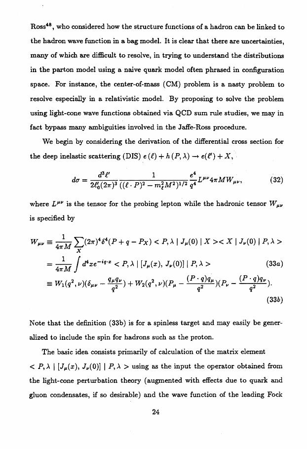
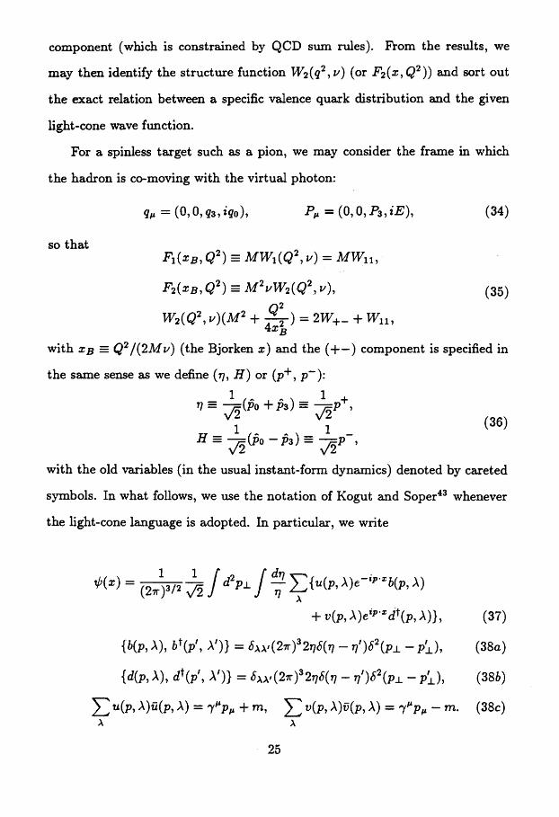
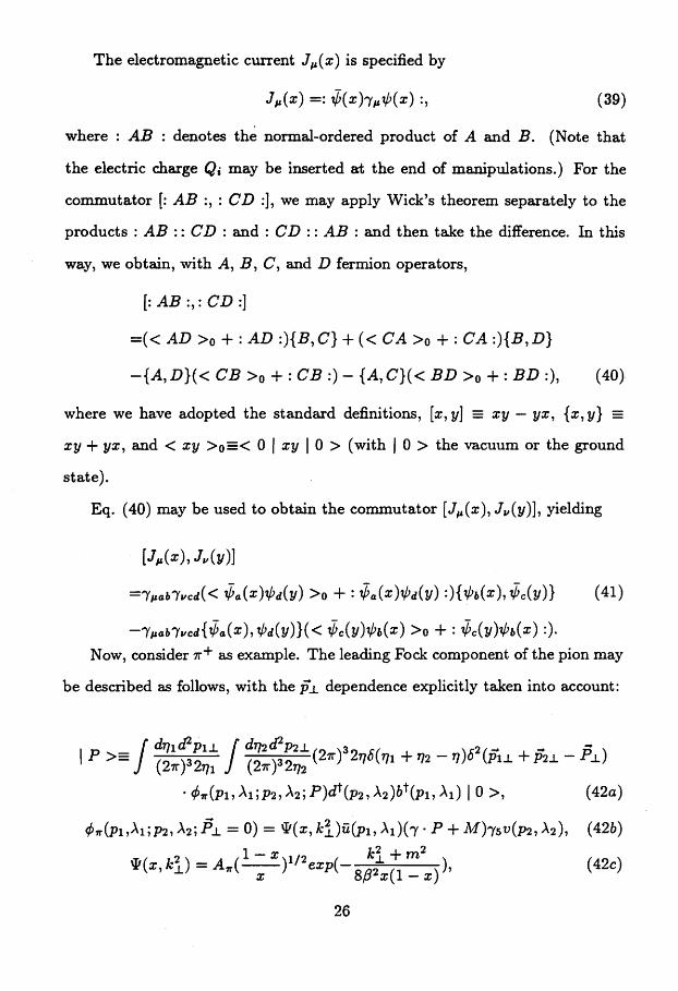
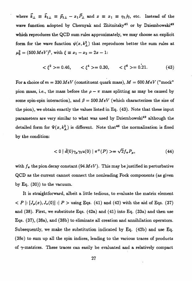
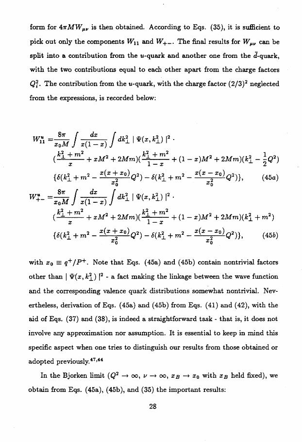
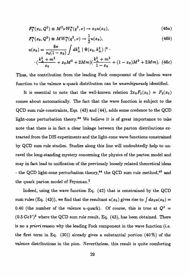
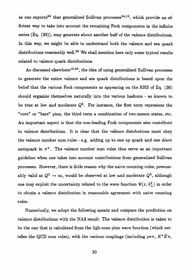
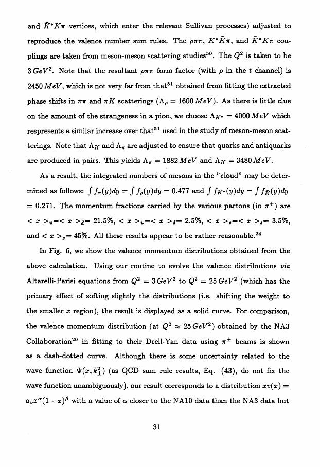
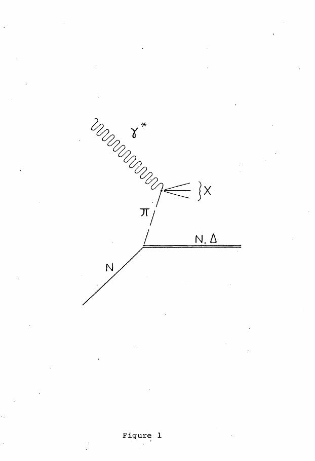
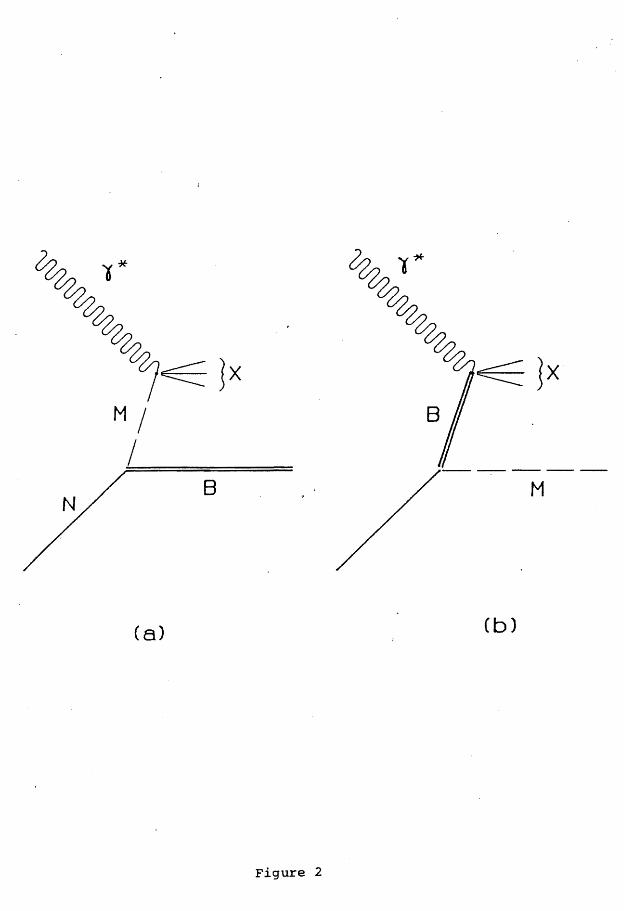
0
M
B
(b)( 8)
Figure 2
bull bull
bull -It-shy
n o
bull
M
N Q)X H
0 s f 11
o
ttl N 0 o o o o o o
r
______~~~____~~~~~~~~~~~~~o
bull
I o
N I o
I)
I 0
o
x
~-0 N 0 0 0 0 0 0
I I
N - - 0 0 0 0 N 0 CO to ~
0
0 0 0 0 0
(X)~-=J - (X)~-=J
o
~~~~~~~~~~~~~~~~~~~o
bull
-
I
0 or-
J
bull I I I I I I I
N I
0 or-
LJ)
OJx ~ J tfi
fx4
I
0 q-orshy
poundX) CD q- N 0 NN 0 0 0or- 0r- O 0 0 0 0
0 0 0 0 0 00 0 0 I I
(X)~j - (X)~j
l I t
co o
to o
gtlt p
v
N
o
~
t M N ~
d d 0 0
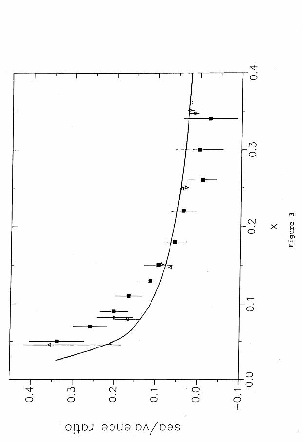
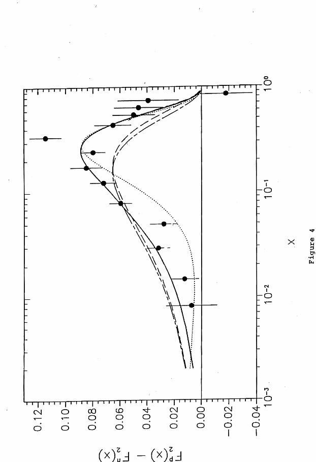
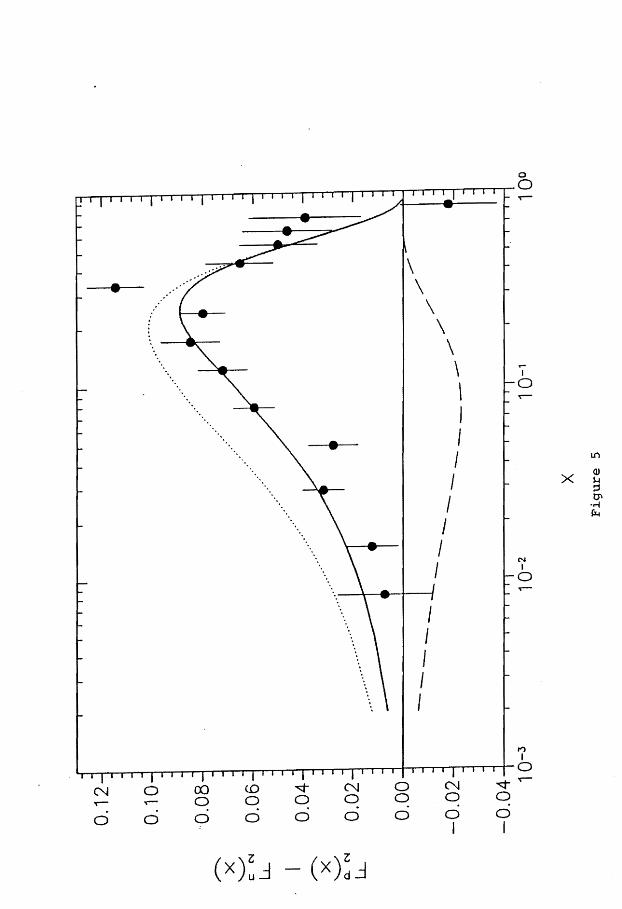
o
~~~~~~~~~~~~~~~~~~~o
bull
-
I
0 or-
J
bull I I I I I I I
N I
0 or-
LJ)
OJx ~ J tfi
fx4
I
0 q-orshy
poundX) CD q- N 0 NN 0 0 0or- 0r- O 0 0 0 0
0 0 0 0 0 00 0 0 I I
(X)~j - (X)~j
l I t
co o
to o
gtlt p
v
N
o
~
t M N ~
d d 0 0
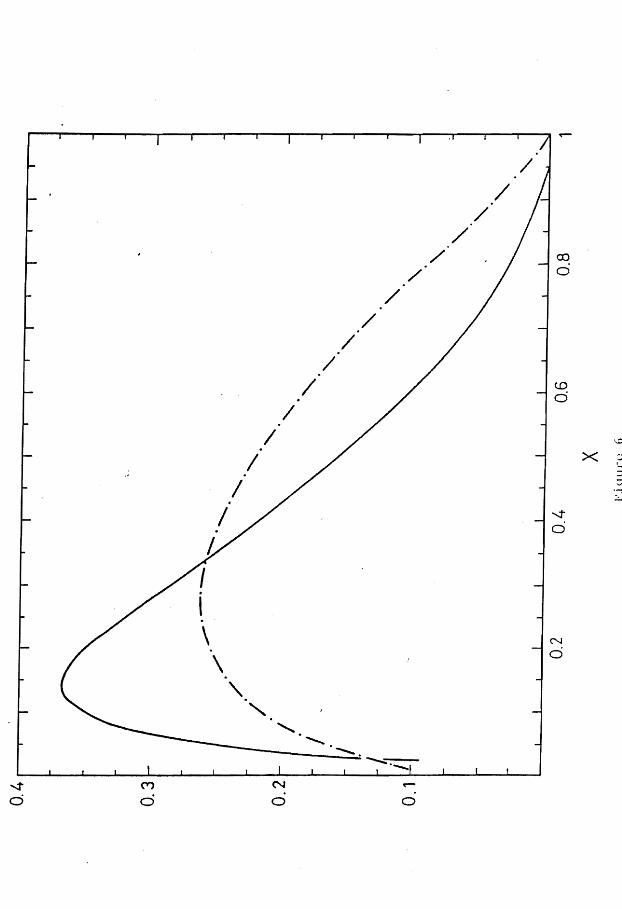
l I t
co o
to o
gtlt p
v
N
o
~
t M N ~
d d 0 0