Embed Size (px)
Citation preview

Toward the next generation of earthquake source models by accounting for model
prediction error
Acknowledgements: Piyush Agram, Mark Simons, Sarah Minson, James Beck,
Pablo Ampuero, Romain Jolivet, Bryan Riel, Michael Aivasis, Hailiang Zhang.
Zacharie DuputelSeismo Lab, GPS division,
Caltech
2
Modeling ingredients‣ Data:
- Field observations- Seismology- Geodesy - ...
‣ Theory: - Source geometry - Earth model - ...
Sources of uncertainty‣ Observational uncertainty:
- Instrumental noise- Ambient seismic noise
‣ Prediction uncertainty: - Fault geometry- Earth model
A posteriori distribution
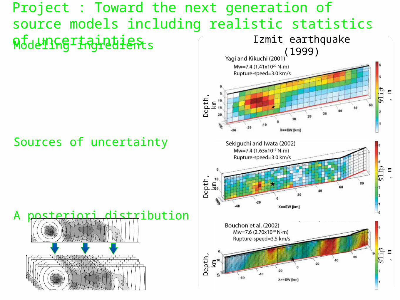
Project : Toward the next generation of source models including realistic statistics of uncertainties
Izmit earthquake (1999)
Dep
th,
kmD
ep
th,
kmD
ep
th,
km
Slip
, m
Slip
, m
Slip
, m
Single model
Ensemble of models
SIV initiative

3
Partial derivatives w.r.t. the elastic parameters (sensitivity
kernel)
Covariance matrix describing uncertainty
in the Earth model parameters
Exact theory
Stochastic (non-deterministic) theory
A reliable stochastic model for the prediction uncertainty
The forward problem‣ posterior distribution:
p(d|m) = N(d | g( ,m), Cp)p(d|m) = δ(d - g( ,m))
Calculation of Cp based on the physics of the problem: A perturbation approach

Covariance
Cμ
Cp
Prediction uncertainty due to the earth model
1000 stochastic realizations

?
Slip, m
H
Dep
th /
H
2H
μ1
μ2
μ2/μ1 =1.4
0.9H
- Data generated for a layered half-space (dobs)
- 5mm uncorrelated observational noise (→Cd)
- GFs for an homogeneous half-space (→Cp)
- CATMIP bayesian sampler (Minson et al., GJI
2013):
Toy model 1: Infinite strike-slip fault
Slip, m
H
Dep
th /
H
2H
μ2
0.9H
Synthetic Data + Noiseshallow fault + Layered half-
space
Inversion:Homogeneous half-space
μ1
μ2

Toy model 1: Infinite strike-slip fault
Input (target) model
Posterior Mean Model

Slip, m
Slip, m
Depth
/
H
Dis
pla
cem
en
t, m
Distance from fault / H
No Cp (overfitting)
Cp Included (larger residuals)
Depth
/
H
Why a smaller misfit does not necessarily indicate a better solution
Distance from fault / H
Dis
pla
cem
en
t, m

8
Toy Model 2: Static Finite-fault modeling
Dist. along Strike, km
Dis
t. a
long D
ip,
km
East, km
Nort
h,
km
Shear modulus, GPa
Depth
, km
Horizontal Disp., m
Vertical Disp., m
Slip, m
Input (target) model
Earth model
Data
Finite strike-slip fault‣ Top of the fault at 0 km‣ South-dipping = 80°‣ Data for a layered half-space

9
Toy Model 2: Static Finite-fault modeling
Dist. along Strike, km
Dis
t. a
long D
ip,
km
East, km
Nort
h,
km
Shear modulus, GPa
Depth
, km
Horizontal Disp., m
Vertical Disp., m
Slip, m
Input (target) model
Earth model
Data
Model for
Data
Model forGFs
Finite strike-slip fault‣ 65 patches, 2 slip components‣ 5mm uncorrelated noise
(→Cd)‣ GFs for an homogeneous half- space (→Cp)
10
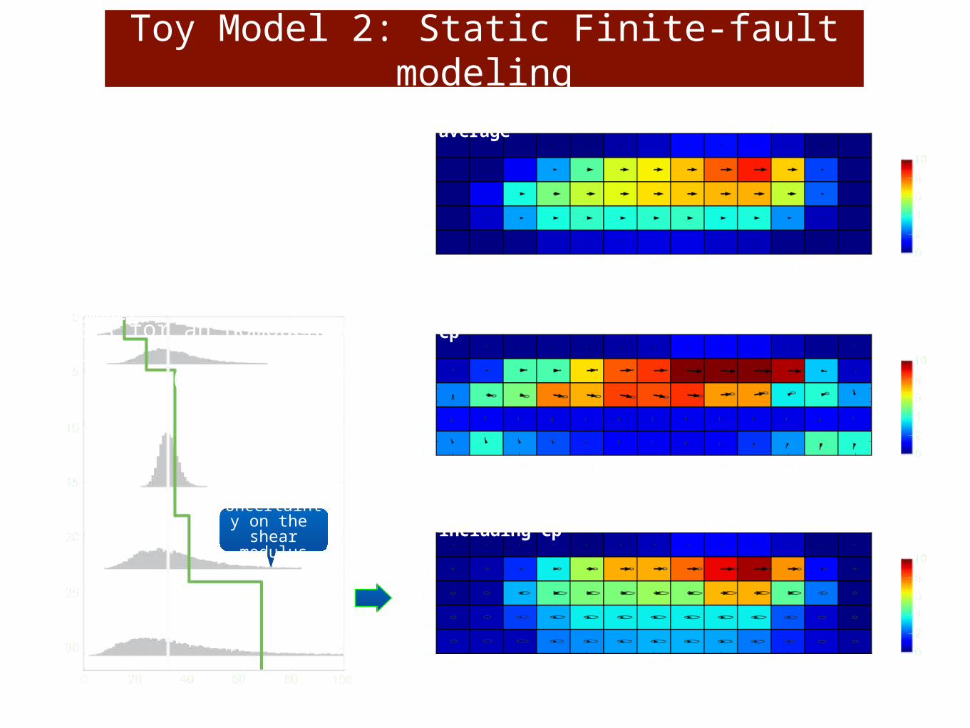
Toy Model 2: Static Finite-fault modeling
Dist. along Strike, km
Dis
t. a
long D
ip,
km
Shear modulus, GPa
Depth
, km
Slip, mFinite strike-slip fault‣ 65 patches, 2 slip components‣ 5mm uncorrelated noise
(→Cd)‣ GFs for an homogeneous half- space (→Cp)
Input (target) model - 65 patches average
Earth model
Dist. along Strike, km
Dis
t. a
long D
ip,
km
Slip, m
Posterior mean model, No Cp
Dist. along Strike, km
Dis
t. a
long D
ip,
km
Slip, m
Posterior mean model, including Cp
Uncertainty on the shear
modulus

Conclusion and Perspectives
Improving source modeling by accounting for realistic uncertainties
‣2 sources of uncertainty-Observational error-Modeling uncertainty
‣Importance of incorporating realistic covariance components-More realistic uncertainty estimations- Improvement of the solution itself
‣Accounting for lateral variations
‣Improving kinematic source models

Jolivet et al., submitted to BSSAAGU Late breaking session on Tuesday
Application to actual data: Mw 7.7 Balochistan earthquake

13
Toy Model 2: Static Finite-fault modeling
Shear modulus, GPa
Depth
, km
Finite strike-slip fault‣ 65 patches, 2 slip components‣ 5mm uncorrelated noise
(→Cd)‣ GFs for an homogeneous half- space (→Cp)
Earth model
Uncertainty on the shear
modulus
Dist. along Strike, km
Dis
t. a
long D
ip,
km
Slip, m
Posterior mean model, including Cp
CpEast(xr), m2
x 104
East, km
Nort
h,
km
Covariance with respect to xr
xr

14
Toy Model 2: Static Finite-fault modeling
Log(μi / μi+1)
Depth
, km
Finite strike-slip fault‣ 65 patches, 2 slip components‣ 5mm uncorrelated noise
(→Cd)‣ GFs for an homogeneous half- space (→Cp)
Earth model
Dist. along Strike, km
Dis
t. a
long D
ip,
km
Slip, m
Posterior mean model, including Cp
CpEast(xr), m2
x 104
East, km
Nort
h,
km
xr
Covariance with respect to xr
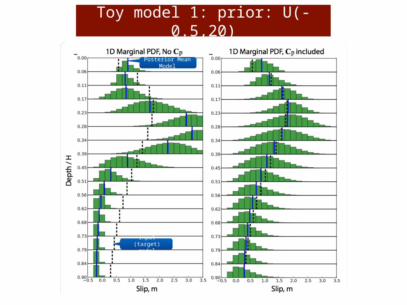
Toy model 1: prior: U(-0.5,20)
Input (target) model
Posterior Mean Model
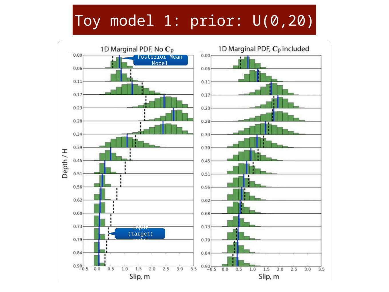
Input (target) model
Posterior Mean Model
Toy model 1: prior: U(0,20)

Toy model including a slip step

Toy model including a slip step

Evolution of m at each beta step
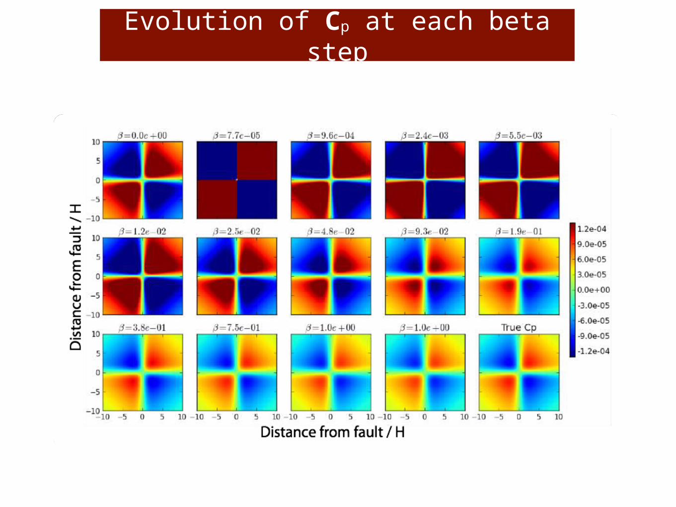
Evolution of Cp at each beta step

Covariance Cμ
1000 realizations

Covariance Cp
1000 realizations

Measurement
errors
Prediction
errors
Observational error:
‣ Measurements dobs : single realization of a stochastic variable d* which can be described by a probability density p(d*|d) = N(d*|d, Cd)
Prediction uncertainty: where Ω = [ μT , φT ]T
‣ Ωtrue is not known and we work with an approximation‣ The prediction uncertainty:
‣ scales with the with the magnitude of m‣ can be described by p(d|m) = N(d | g( ,m), Cp)
A posteriori distribution:
‣ In the Gaussian case, the solution of the problem is given by:
Earthmode
l
Sourcegeometr
y
Measurements
Displacement field
Prior information
On the importance of Prediction uncertainty
D: Prediction space

![Ji. ]s, fr&, No. Lower Agram Road, Agram Post, Bangalore ...pcdablr.gov.in/circular/ltc_clarification_08092017.pdf · VERY I M PORTANT CI RCU LAR gTsIIoI Office of the Principal Controller](https://img.pdfslide.us/doc/110x75/5fc94c90fbf01b634b0bfef9/ji-s-fr-no-lower-agram-road-agram-post-bangalore-very-i-m-portant.jpg)