Toward altimetric data assimilation in a Tropical Atlantic ...horizon.documentation.ird.fr/exl-doc/pleins_textes/pleins_textes_6/... · JOURNAL OF GEOPHYSICAL RESEARCH, VOL. 97, NO

JOURNAL OF GEOPHYSICAL RESEARCH, VOL. 97, NO. C12, PAGES 20,271-20,283, DECEMBER 15, 1992

Toward Altimetric Data Assimilation in a Tropical Atlantic Model

BERNARD BOURLES

Centre ORSTOM de .Cayenne, French Guiana

SABINE ARNAULT

Laboratoire d‘océanographie Dynamique et de Climatologie, ORSTOM, Université Paris VI, Paris

CHRISTINE PROVOST

Laboratoire d‘océanographie Dynamique et de Climatologie, CNRS, Université Paris VI, Paris

We present three types of experiments of sequential assimilation of altimetric data in a linear tropical Atlantic model, using an analysis technique we developed. In the first experiments we assimilate dynamic height fields calculated from simulated data in order to study the impacts of assimilations. In the second ones we assimilate dynamic height anomaly fields calculated from simulated data, and finally, in the third ones we use sea level anomaly fields obtained from altimetric data from Geosat. Perturbations are observed in the eastern part of the basin, due to Kelvin waves artificially generated in the west equatorial basin. However, we show that altimetic data may be very useful for improving model simulations in the tropics when appropriate assimilation techniques are used.

1. INTRODUCTION

The 1982-1983 “El Nino,” which strongly perturbed the climate as far as the mid-latitudes, has confirmed that tropical oceans play a major role in the observed climate variability [Merle and Gillet, 19851. Nowadays, oceanic tridimensional models describe fairly well the tropical circulation [Philander aiid Pacanowski, 1984, 1986; Morlière et al., 19891. However, as the accuracy of the atmospheric forcings and of the initial conditions is still limited, oceanic state simulations are not precise enough for prediction by using coupled “ocean-atmosphere” models. Therefore it is necessary to mix all available informations (data, statistics, model results, etc) to provide the most complete and precise state of the ocean, and data assimilation techniques could be useful for doing that. They have been used for a long time in meteorology, but their studies are quite recent in tropical oceans. First experiments in the tropical Pacific and the Indian oceans, using in situ data, have shown encouraging results [Moore et al., 1987; Leetina and Ji, 1989; Morlière et al., 19891.

Contrary to in situ data, satellite data can provide high spatial resolution and quasi-synoptic views of the sea surface of the oceans, and recent studies indicate that satellite altimetric data may be very helpful for the study of the large-scale low-frequency variations of the tropical oceans [Miller et al., 1986;. Ménard, 1988; Arnault et al., 1989, 19901. Thus we have chosen to assimilate altimetric data, obtained from the U.S. Navy Geosat satellite, in a simple linear model of the tropical Atlantic Ocean [Delécluse, 1984; Arnault, 19841. When considering satellite data for assimilation, specific problems can arise: aliasing due to the data coverage, weak signal amplitude, relationship between model

Copyright 1992 by the American Geophysical Union.

variables and satellite data, etc. Thus numerical experiments are necessary before assimilating actual altimetry. In section 2 we present the linear model that we use and

the assimilation technique that we developed for this study. In section 3 we describe preliminary studies of the impact of synthetic dynamic height assimilation in the model. Then we assimilate synthetic dynamic height anomalies, which are directly related to the sea level anomalies obtained from altimetric data. In section 4 we describe the altimetric data used and we discuss the results of their assimilation in the linear model, before concluding. Results obtained may be helpful in the approach of an operational hindcasting of the ocean state, which is one of the objectives of the Tropical Ocean Global Atmosphere (TOGA) program.

2. THE MODEL AND THE ASSIMILATION TECHNIQUE

2.1. The Model

Altimetric data give information on the sea level anomaly. Due to the baroclinic character of the tropical Atlantic Ocean, the sea level anomaly can be compared, in a first approach, to dynamic height anomaly, which characterizes fairly well the dynamic state of the ocean. We may compute mean geostrophic currents and estimate the heat content variability over the subthermoclinal layer from these dynamic height anomaly fields [Delcroix and Gautier, 19871.

Thus we need a model which reliably reproduces dynamic height variations and which is not costly in computing time so that various numerical experiments can be undertaken. Dif€erent studies have shown the ability of linear vertical mode models to reproduce the seasonal variability of dynamic height [Du Penhoat and Tréguier, 19851. The linear vertical mode model developed by Delécluse [1984] and Arnault [1984] is one possible choice.

Philander et al. [19871 have shown that mass fields seem to produce better results than velocity fields when assimilated in their general circulation model. However, analytical and paper lumber 92Jc01507. p 1. S.T. Q. &I* Fofida ~ ~ ~ ~ ~ ~ f l ~ ~ ~ ~ ~

8‘6 20,271

0148-0227/92/92JC-01507$0 .O

2 7 AOLU 1993

20,272 BOURLES ET AL.: TOWARD ALTIMETRIC DATA ASSIMILATION IN A TROPICAL MODEL

* + + + + + + + + + + + + + + + + + + + + + + + + + + + + + + + + + + + + + + . . . . . . . . . . . . . . . . . . . . . . . . . * + + + + + + + + + + + + + + + + + + + + + + + + + + + + + + + + + + + t + + + + + + + + + + + + + + + + *++t+++++t + + + + + + + + + + + t + + + + + + + + + t + + + + + + + + + + + + + + + + + + + . . . . . . . . . . . . . . . . . . . . . . + + + + + + + + + + + + + + + + + + + + + + + i. + + + + + + + + + + + + + + + + + + . . . . . . . . . . . . . . . . . . . . . . . . . . . . . . . . . . . . . . . . . . + + + + + + + + + + + + + . . . . . . . . . . . . . . . . . . . . . . . . . . . . * + + + + + + + t + + + + + + + + + + + + + + + + + + + + + + + + + + + + + + + + + + + + + t + + + t + +ti+++++++ i + + + + + + + + + + + + + + + + + + + + + + t + + + + + + + + + + + + + + + + + + + + + ++++++++*++++++++ + + + + + + + + + + + + + + + + + + + + + + + + + + + + + + + + + + + + + + + . . . . . . . . . . . . . . . . . . . . . . . *+++++++++i + + + + + + + + + + + + + + + + + + + + + + + + ++++i+ + . . . . . . . . . . . . . . . . . . . .

TotalEnergy - Potential Energy - Kinetic Energy .....

.+. Wind Forcing

2oo 1

1 2 3 4 ? 6 7 I p Time (years)

5

4

"?

N' 2 E

2 1 .5

.5 r O P

M

U

-1 3 -2

-3

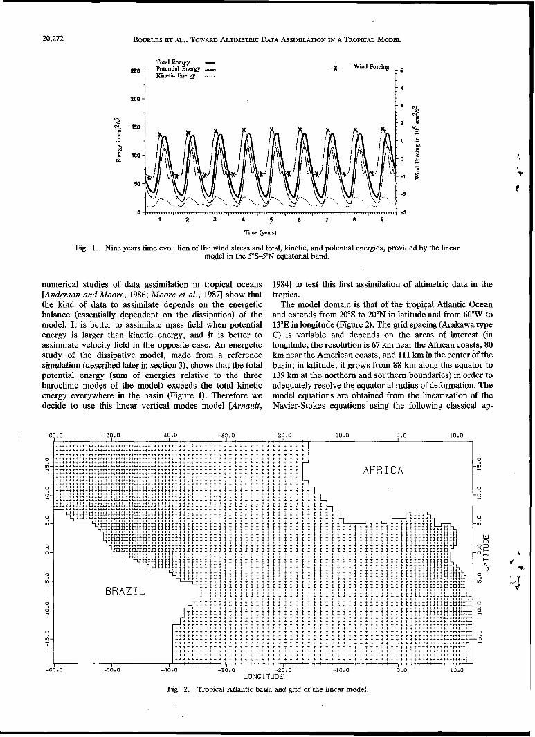
Fig. 1. Nine years time evolution of the wind stress and total, kinetic, and potential energies, provided by the linear model in the 5"S-Y'N equatorial band.

numerical studies of data assimilation in tropical oceans [Anderson und Moore, 1986; Moore et al., 19871 show that the kind of data to assimilate depends on the energetic balance (essentially dependent on the dissipation) of the model. It is better to assimilate mass field when potential energy is larger than kinetic energy, and it is better to assimilate velocity field in the opposite case. An energetic study of the dissipative model, made from a reference simulation (described later in section 3), shows that the total potential energy (sum of energies relative to the three baroclinic modes of the model) exceeds the total kinetic energy everywhere in the basin (Figure 1). Therefore we decide to use this linear vertical modes model [Arnault,

19841 to test this first assimilation of altimetric data in the tropics.

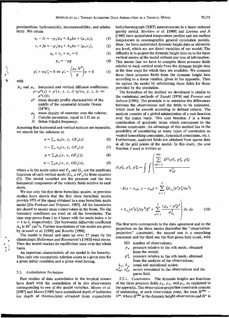
The model domain is that of the tropical Atlantic Ocean and extends from 20"s to 20"N in latitude and from 60"W to 13"E in longitude (Figure 2). The grid spacing (Arakawa type C) is variable and depends on the areas of interest (in longitude, the resolution is 67 km near the African coasts, 80 km near the American coasts, and I l 1 km in the center of the basin; in latitude, it grows from 88 km along the equator to 139 km at the northern and southern boundaries) in order to adequately resolve the equatorial radius of deformation. The model equations are obtained from the linearization of the Navier-Stokes equations using the following classical ap-

l

o 2

O

O

o 10

o

O

10 I

o. O

I - o Y

AFR I CA

BOURLES ET AL.: TOWARD ALTIMETRIC DATA ASSIMILATION IN A TROPICAL MODEL 20,273

proximations: hydrostaticity , incompressibility, and adiaba- ticity. We obtain

(1) U t -fu = -Px/PO + AhAu + (puuz)z

p ; + w p * , = o = P P ; - (pogN2)w - = o ( 5 )

with

Ah and pV horizontal and vertical dausion coefficients. P‘P*(Z) + P ‘ ( X , Y , z , t ) ( P ’ ( X , Y , z , t ) <<

p*(z>); p* mean density profile characteristic of the

middle of the equatorial Atlantic Ocean (24”W);

po mean density of seawater over the column; f Coriolis parameter, equal to 2 i2 sin (o;

N Briint-Väisälä frequency. Assuming that horizontal and vertical motions are separable, we search for the solutions as

U = 6, un(x, Y , t )Fn(z)

= C n Vu, (x , Y , t)Fn(z)

P = GnPs,(x, Y , t)Fn(z)

(6)

(7)

(8)

= C n w n ( X , Y , t )Gn(z) , (9)

where n is the mode index and F , and G, are the amplitude functions of each vertical mode (G, CY aF,/az from equation (3)) . The model variables are the pressure and the two horizontal components of the velocity fields relative to each mode.

We use only the first three baroclinic modes, as previous studies have shown that the first three baroclinic modes provide 95% of the signal obtained in a nine baroclinic mode model [Du Penhoat and Tréguier, 19851. AU the boundaries are closed to ensure mass conservation in the basin. No slip boundary conditions are used on all the boundaries. The time step grows from 1 to 4 hours with the mode index n (n = 1 to 3, respectively). The horizontal dausivity coefficient Ah is lo7 Cm2/s. Further descriptions of this model are given by Arnault et al. [1990] and Bourlès [1990].

The model is forced and spun up over 17 years by the climatologic Hellerman and Rosenstein’s [ 19831 wind stress. Then the model reaches its equilibrium state over the whole basin.

An important characteristic of our model is the linearity. Thus only one assymptotic solution exists at a given time for a given initial condition and a given wind forcing.

2.2. Assimilation Technique

Past studies of data assimilation in the tropical oceans have dealt with the assimilation of in situ observations corresponding to one of the model variables. Moore et al. [1987] and Moore 119891 have assimilated depth of isotherms (or depth of thermocline) obtained from expendable

bathythermograph (XBT) measurements in a linear reduced gravity model. Morlière et al. [1989] and Leetma and Ji [ 19891 have assimilated temperature profiles and sea surface temperature in oceanographic general circulation models. Here, we have assimilated dynamic height data or altimetric sea level, which are not direct variables of our model. The difficulty is to project the dynamic height data on to the three vertical modes of the model without any loss of information. This means that we have to compute three pressure fields relative to each vertical mode from the dynamic height data at the time steps for which they are available. We compute these three pressure fields from the dynamic height data according to a linear relation, given in the appendix. Then we update the model by substituting these fields for those provided by the simulation.

The formalism of the method we developed is similar to the variational methods of Sasaki [1970] and Provost and Salinon [1986]. The principle is to minimize the daerences between the observations and the fields to be estimated, which must be smooth according to defined criteria. The analysis consists of a global minimization of a cost function over the entire basin. This cost function J is a linear combination of quadratic terms which correspond to the chosen constraints. An advantage of this method lies in the possibility of considering as many types of constraints as wanted (smoothing constraints, dynamical constraints, etc.). Furthermore, analyzed fields are obtained from sparse data at all the grid points of the model. In this study, the cost function J used is written as

3

n = 1

The first term corresponds to the data agreement and to the projection on the three modes (hereafter the “observation- projection” constraint), the second one is a smoothing constraint and the third one the first guess field recall, with

ND number of observations; p n pressure relative to the nth mode, obtained

from the model; p*, pressure relative to the nth mode, obtained

from the analysis of the observations; zonal and meridional scales;

guess field.

L,, L Und, 2 - 2 ffP, errors associated to the observations and the

2.2.1. Constraints. The dynamic heights are functions of the three pressure fields p 1, p 2 , and p 3 , as explained in the appendix. The observation-projection constraint consists of minimizing, at each observation point, the term Hobs - H*, where Hobs is the dynamic height observation and H* is


the bilinear interpolation at the observation point of the dynamic heights obtained at the four closest grid points surrounding the observation point:

D ( p ; , p ; , p ; ) = Hobs(xobs, yobs) - H,f+ Ho

3 4

n = 1 i = l

where i is the index of the four grid points surrounding the observation, n is the mode index, and KA is a coefficient depending on the modes and the interpolation. This constraint takes into account the errors aid associated with the observations. The computation of these errors is explained in the section 3.

The anisotropy of the fields, which is very pronounced in the tropics, is taken into account in the smoothing constraint where we consider the zonal and meridional correlation lengths L, and L, in the two respective components of the horizontal Laplacian. The correlation lengths (zero crossing of the spatial autocorrelation functions at each grid point) computed from the model dynamic height fields or the three pressure fields relative to each mode are very similar: for each field (dynamic height or pressure), L, decreases iden- tically from about 2000 km along the equator to 800 km in high latitudes and L, grows from about 300 km in the center of the basin to 1000 km close to the African and South American coasts. Consequently, we will not consider different LXn or LYn correlation scales for each mode but only use the L, and L, scales computed from the model dynamic height fields.

The guess field recall constraint takes into account the errors u;,, associated with the three pressure fields of the model. As these fields are numerical model results, the determination of the errors is relatively arbitrary. For each pressure field, we estimate errors as equal to the time-space variance added to 1/10 of the time variability. Thus we obtain three estimated error fields constant with time and the errors

' are supposed more important in the areas with strong variability.

2.2.2. Assimilation process and analysis errors. The cost function J is minimized according to the searched fields pTI. We obtain a system of NMXNPT linear equations (NM, number of modes; NPT, number of grid points of the model). This system is written in a matrix form A X = B , where A is a positive and very sparse square matrix, X is the column vector of unknowns p*, , and B depends on the observations. This system is solved by a conjugate gradient method, accelerated by block symmetric overrelaxation [Provost, 19831.

When data are available, the assimilation processing consists of (1) stopping the simulation of the linear model, (2) proceeding to the analysis, and (3) substituting the fields p*, obtained from the analysis for the three pressure fields p n (the guess field). Then we restart the simulation and the linear model is only driven by the monthly wind stress, until the next update.

First experiments (not described here) have shown that (1) a Newtonian progressive data assimilation scheme (over several time steps) does not provide improvements compared to a brutal replacement scheme (over only one time step), when pressure fields are assimilated over the entire

basin; on the other hand, to avoid strong time-space gradi- ents around the data point, a Newtonian scheme has to be chosen when fields are assimilated in limited areas of the basin, and (2) the velocity field is very quickly adjusted after each updating, due to the large dissipation coefficient of the model, and has no effects on the mass field response to the assimilations.

As the model is linear, the analysis errors may be easily estimated. The analyzed field variations 6X relative to the guess field X & and to the observations Hobs can be computed according to

SX 6B 6 X 6B -- - A-' - and -= A-' - 8Xgf 6 X d 6HobS 6 H ObS

Then, the analysis error AX is obtained from

where A$ and Ags are the guess field and observation errors, respectively.

This computation is made simultaneously with the analysis, the inverted matrix being the same as in the analysis.

3. ASSIMILATION OF SYNTHETIC DYNAMIC HEIGHT AND DYNAMIC HEIGHT ANOMALY FIELDS

In this section, we observe the response of the linear model to assimilation on a seasonal time scale. We define the "data retention" of the model as the period during which the model retains the information provided by the past updates. To reproduce the global and quasi-synoptic coverage obtained from satellite data, we have first considered simulated data issued from the climatological run of the Geophysical Fluid Dynamic Laboratory (GFDL) model, forced by the Hellerman and Rosenstein's [1983] wind stress fields [Phi- lander and Pacanowski, 19841. Temperature and salinity are obtained at all the vertical levels and all the grid-points of this model, on the fifteenth of each month. Corresponding dynamic height fields were computed from these data using the state equation as that of Miller0 and Poisson [1981]. These dynamic height fields are computed from 5 dbar (first vertical level of the GFDL model) to 500 dbar, and they are used as observations in assimilation experiments. The model, forced by the same climatological wind stress, is equilibrated after the seventeenth year of simulation which is used as control run (CR).

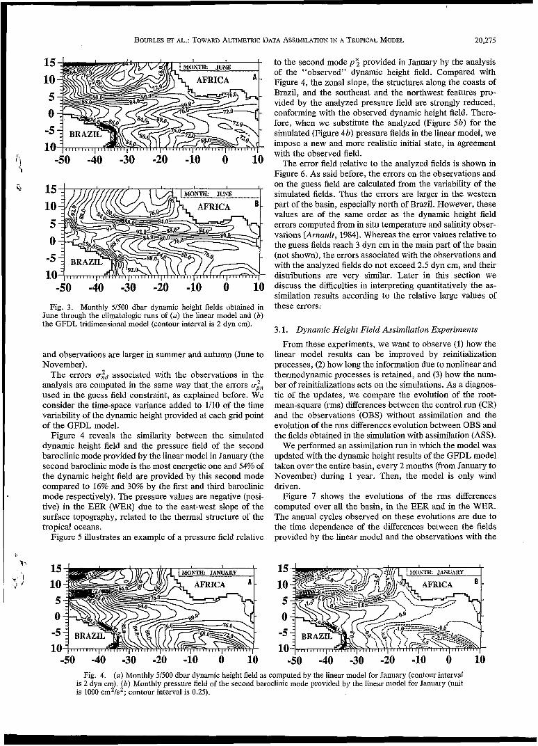
The dynamic height fields obtained from the linear model are, except off the north Brazilian coasts, lower than those issued from the simulation of the GFDL model (from now on called "observations"). As illustrated in Figure 3b, the linear model overestimates the equatorial slope, the values being lower in the East Equatorial Region (EER) and larger in the West Equatorial Region (WER). This overestimation of the equatorial gradient is maximum in autumn and reaches 25 dyn cm in October (not shown). In the southern hemisphere, both models simulate ridges and troughs, which are not located at the same latitudes and are out of phase during the entire year. The linear model strongly overestimates the troughs obtained in the . northwest (35"W-10"N) and the southeast (o"E-lO"S), mainly because of the vicinity of the closed boundaries. Differences between our model results


-50 -40 -30 -io -io o i o

15 10 5 O

-5 10

-50 -40 -30 -20 -10 O 10 Fig. 3. Monthly 5/500 dbar dynamic height fields obtained in

June through the climatologic runs of (u) the linear model and (b) the GFDL tridimensional model (contour interval is 2 dyn cm).

and observations are larger in summer and autumn (June to November).

The errors a i d associated with the observations in the analysis are computed in the same way that ,the errors used in the guess field constraint, as explained before. We consider the time-space variance added to 1/10 of the time variability of the dynamic height provided at each grid point of the GFDL model.

Figure 4 reveals the similarity between the simulated dynamic height field and the pressure field of the second baroclinic mode provided by the linear model in January (the second baroclinic mode is the most energetic one and 54% of the dynamic height field are provided by this second mode compared to 16% and 30% by the first and third baroclinic mode respectively). The pressure values are negative (positive) in the EER (WER) due to the east-west slope of the surface topography, related to the thermal structure of the tropical oceans.

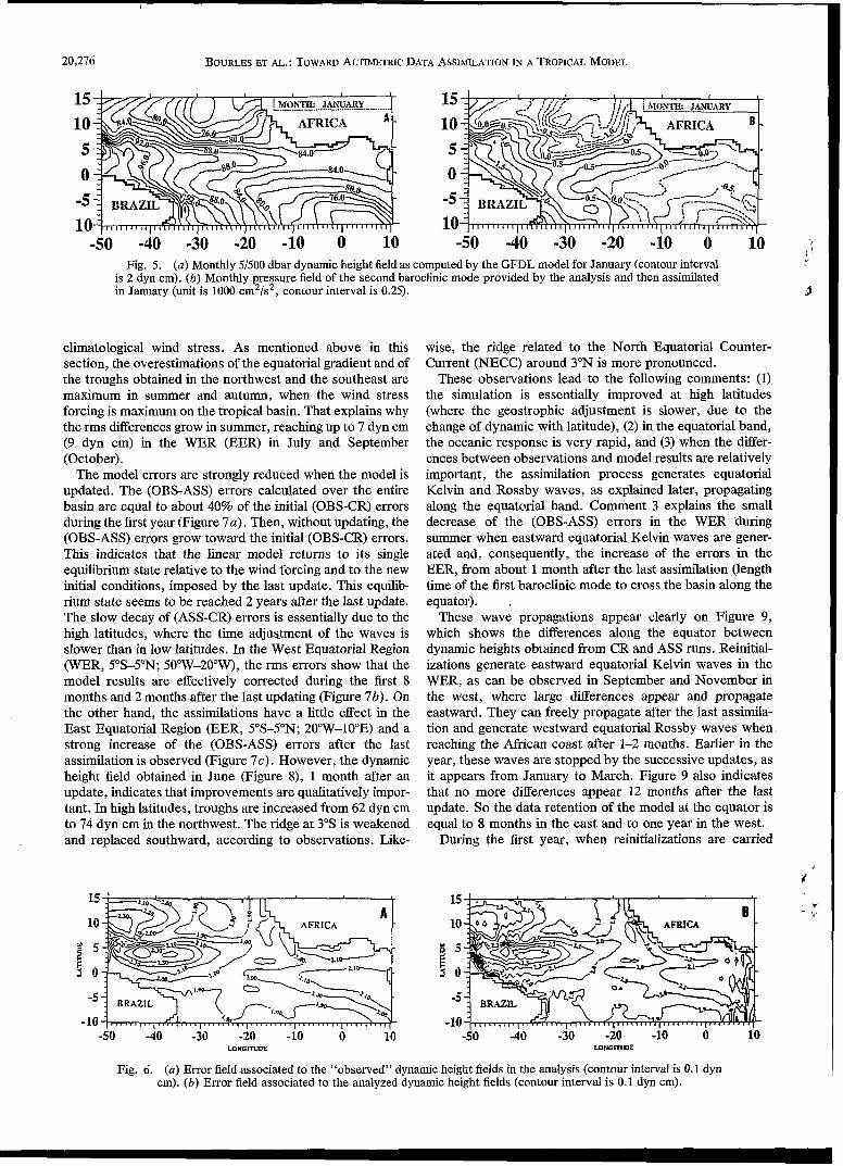
Figure 5 illustrates an example of a pressure field relative

-50 -40 -30 -io -io o io

to the second mode p ; provided in January by the analysis of the "observed" dynamic height field. Compared with Figure 4, the zonal slope, the structures along the coasts of Brazil, and the southeast and the northwest features provided by the analyzed pressure field are strongly reduced, conforming with the observed dynamic height field. There- fore, when we substitute the analyzed (Figure 5b) for the simulated (Figure 4b) pressure fields in the linear model, we impose a new and more realistic initial state, in agreement with the observed field.

The error field relative to the analyzed fields is shown in Figure 6. As said before, the errors on the observations and on the guess field are calculated from the variability of the simulated fields. Thus the errors are larger in the western part of the basin, especially north of Brazil. However, these values are of the same order as the dynamic height field errors computed from in situ temperature and salinity observations [Arnault, 19841. Whereas the error values relative to the guess fields reach 3 dyn cm in the main part of the basin (not shown), the errors associated with the observations and with the analyzed fields do not exceed 2.5 dyn cm, and their distributions are very similar. Later in this section we discuss the difliculties in interpreting quantitatively the assimilation results according to the relative large values of these errors:

3.1. Dynamic Height Field Assimilation Experiments

From these experiments, we want to observe (1) how the linear model results can be improved by reinitialization processes, (2) how long the information due to nonlinear and thermodynamic processes is retained, and (3) how the number of reinitializations acts on the simulations. As a diagnos- tic of the updates, we compare the evolution of the root- mean-square (rms) diffaences between the control run (CR) and the observations (OBS) without assimilation and the evolution of the rms dzerences evolution between OBS and the fields obtained in the simulation with assimilation (ASS).

We performed an assimilation run in which the model was updated with the dynamic height results of the GFDL model taken over the entire basin, every 2 months (from January to November) during 1 year. Then, the model is only wind driven.

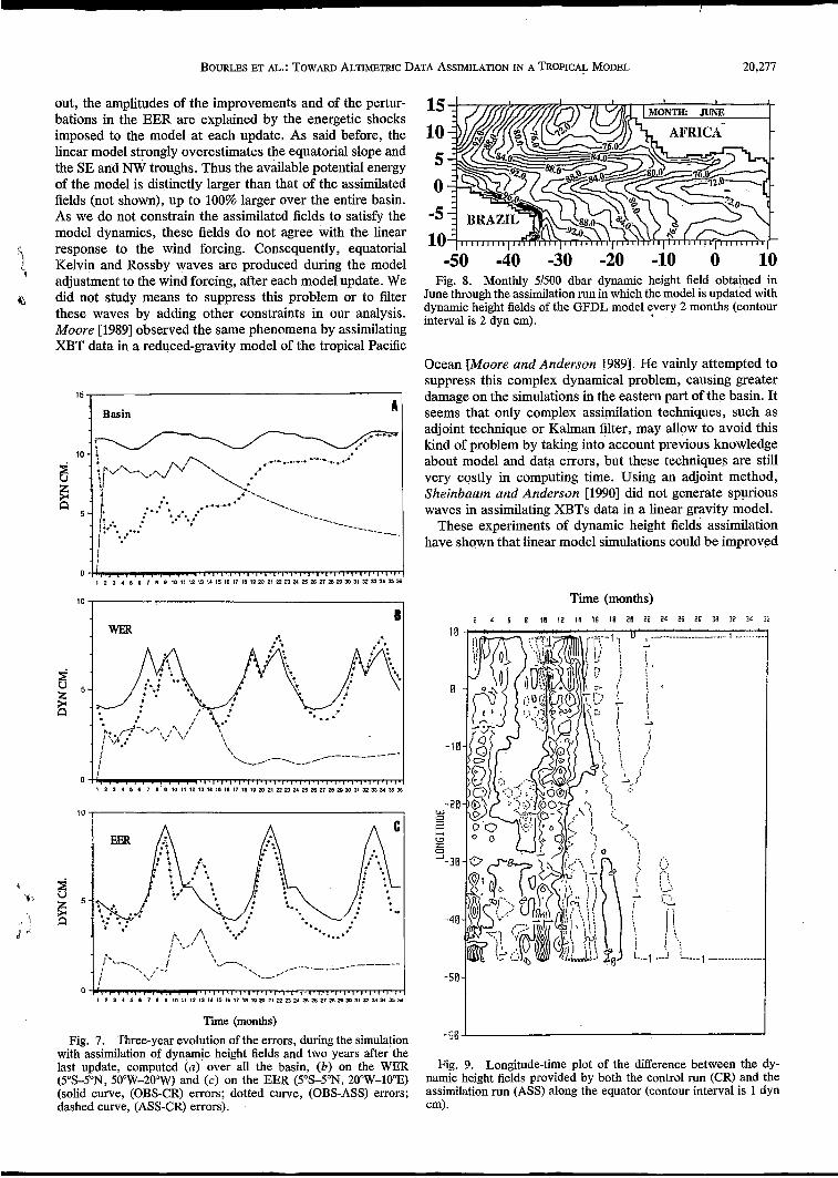
Figure 7 shows the evolutions of the rms differences computed over all the basin, in the EER and in the WER. The annual cycles observed on these evolutions are due to the time dependence of the differences between the fields provided by the linear model and the observations with the

-50 -40 -30 -20 -io o 10 Fig. 4. (u) Monthly Y500 dbar dynamic height field as computed by the linear model for January (contour interval

is 2 dyn cm). (b) Monthly pressure field of the second baroclinic mode provided by the linear model for January (unit is 1000 cm2/s2; contour interval is 0.25).

20,276 BOURLES ET AL.: TOWARD ALTIMETIUC DATA ASSIMILATION IN A TROPICAL MODEL

15 15 10 10 5 5 O O

-5 -5 10 10

-50 -40 -30 -20 -10 O 10 -50 -40 -30 -20 -10 O 10 Fig. 5. (u) Monthly 5/500 dbar dynamic height field as computed by the GFDL model for January (contour interval

is 2 dyn cm). (b ) Monthly pressure field of the second baroclinic mode provided by the analysis and then assimilated in January (unit is 1000 cm2/s2, contour interval is 0.25).

climatological wind stress. As mentioned above in this section, the overestimations of the equatorial gradient and of the troughs obtained in the northwest and the southeast are maximum in summer and autumn, when the wind stress forcing is maximum on the tropical basin. That explains why the rms differences grow in summer, reaching up to 7 dyn cm (9 dyn cm) in the WER (EER) in July and September (October).

The model errors are strongly reduced when the model is updated. The (OBS-ASS) errors calculated over the entire basin are equal to about 40% of the initial (OBS-CR) errors during the first year (Figure 7a). Then, without updating, the (OBS-ASS) errors grow toward the initial (OBS-CR) errors. This indicates that the linear model returns to its single equilibrium state relative to the wind forcing and to the new initial conditions, imposed by the last update. This equilibrium state seems to be reached 2 years after the last update. The slow decay of (ASS-CR) errors is essentially due to the high latitudes, where the time adjustment of the waves is slower than in low latitudes. In the West Equatorial Region (WER, 5OS-5"N; 5O0W-2O"W), the rms errors show that the model results are effectively corrected during the first 8 months and 2 months after the last updating (Figure 7b). On the other hand, the assimilations have a little effect in the East Equatorial Region (EER, 5OS-5"N; 20"W-10"E) and a strong increase of the (OBS-ASS) errors after the last assimilation is observed (Figure 7c). However, the dynamic height field obtained in June (Figure 8), 1 month after an update, indicates that improvements are qualitatively important. In high latitudes, troughs are increased from 62 dyn cm to 74 dyn cm in the northwest. The ridge at 3"s is weakened and replaced southward, according to observations. Like-

wise, the ridge related to the North Equatorial Counter- Current (NECC) around 3"N is more pronounced.

These observations lead to the following comments: (1) the simulation is essentially improved at high latitudes (where the geostrophic adjustment is slower, due to the change of dynamic with latitude), (2) in the equatorial band, the oceanic response is very rapid, and (3) when the differences between observations and model results are relatively important, the assimilation process generates equatorial Kelvin and Rossby waves, as explained later, propagating along the equatorial band. Comment 3 explains the small decrease of the (OBS-ASS) errors in the WER during summer when eastward equatorial Kelvin waves are generated and, consequently, the increase of the errors in the EER, from about 1 month after the last assimilation (length time of the first baroclinic mode to cross the basin along the equator). ,

These wave propagations appear clearly on Figure 9, which shows the differences along the equator between dynamic heights obtained from CR and ASS runs. Reinitial- izations generate eastward equatorial Kelvin waves in the WER, as can be observed in September and November in the west, where large differences appear and propagate eastward. They can freely propagate after the last assimilation and generate westward equatorial Rossby waves when reaching the African coast after 1-2 months. Earlier in the year, these waves are stopped by the successive updates, as it appears from January to March. Figure 9 also indicates that no more differences appear 12 months after the last update. So the data retention of the model at the equator is equal to 8 months in the east and to one year in the west.

During the first year, when reinitializations are carried

-50 -io -3, -io -io o io LOffiKWE

Fig. 6. (u) Error field associated to the "observed" dynamic height fields in the analysis (contour interval is 0.1 dyn cm). ( b ) Error field associated to the analyzed dynamic height fields (contour interval is 0.1 dyn cm).

BOURLES ET AL.: TOWARD ALTIMETRIC DATA ASSIMILATION IN A TROPIC& MODEL 20,277

out, the amplitudes of the improvements and of the perturbations in the EER are explained by the energetic shocks imposed to the model at each update. As said before, the linear model strongly overestimates the equatorial slope and the SE and NW troughs. Thus the available potential energy of the model is distinctly larger than that of the assimilated fields (not shown), up to 100% larger over the entire basin. As we do not constrain the assimilated fields to satisfy the model dynamics, these fields do not agree with the linear response to the wind forcing. Consequently, equatorial Kelvin and Rossby waves are produced during the model adjustment to the wind forcing, after each model update. We did not study means to suppress this problem or to fìlter these waves by adding other constraints in our analysis. Moore [1989] observed the same phenomena by assimilating XBT data in a reduced-gravity model of the tropical Pacific

, 1

Basin '* 1

0 % , , , , , , , , , i.,.,.,. I . , . , .- i 2 3 4 5 6 7 8 O 1 0 1 1 1 2 1 3 1 1 1 5 ~ 6 1 7 I ~ l D W 2 1 t Z ~ 2 4 ~ 2 s 2 7 ~ 2 0 ~ 3 1 3 2 ~ ~ ~ ~

BI 10

I 2 3 1 5 6 7 8 D 1 0 1 t I 2 I 3 1 I 1 5 1 6 l 7 1 1 1 9 2 0 2 1 2 2 n 2 ~ r X 2 2 7 X 2 0 ~ I I 3 z ~ ~ ~ 1 6

Time (months)

Fig. 7. Three-year evolution of the errors, during the simulation with assimilation of dynamic height fields and two years after the last update, computed (a) over all the basin, ( b ) on the WER (5"S-5"N, 5O"W-2O0W) and (c) on the EER (S0S-5"N, 20"W-WE) (solid curve, (OBS-CR) errors; dotted curve, (OBS-ASS) errors; dashed curve, (ASS-CR) errors).

-So -40 -30 -io -io o 10 Fig. 8. Monthly 51500 dbar dynamic height field obtained in

June through the assimilation run in which the model is updated with dynamic height fields of the GFDL model !very 2 months (contour interval is 2 dyn cm).

Ocean [Moore and Anderson 19891. He vainly attempted to suppress this complex dynamical problem, causing greater damage on the simulations in the eastern part of the basin. It seems that only complex assimilation techniques, such as adjoint technique or Kalman filter, may allow to avoid this kind of problem by taking into account previous knowledge about model and data errors, but these techniques are still very costly in computing time. Using an adjoint method, Sheinbaum and Anderson [1990] did not generate spurious waves in assimilating XBTs data in a linear gravity model.

These experiments of dynamic height fields assimilation have shown that linear model simulations could be improved

Time (months) 2 1 6 8 10 12 11 16 18 20 22 24 26 2K 38 32 31 lb

i a

a

-10

-20 w O 1 c c( W æ

_I a

-38

-46

-58 1 Fig. 9. Longitude-time plot of the dserence between the dy-

namic height fields provided by both the control run (CR) and the assimilation run (ASS) along the equator (contour interval is 1 dyn cm) .


O 2 4 I I II 12 I( I C I l 21 12 14 16 21 II 32 38 16

Time (months)

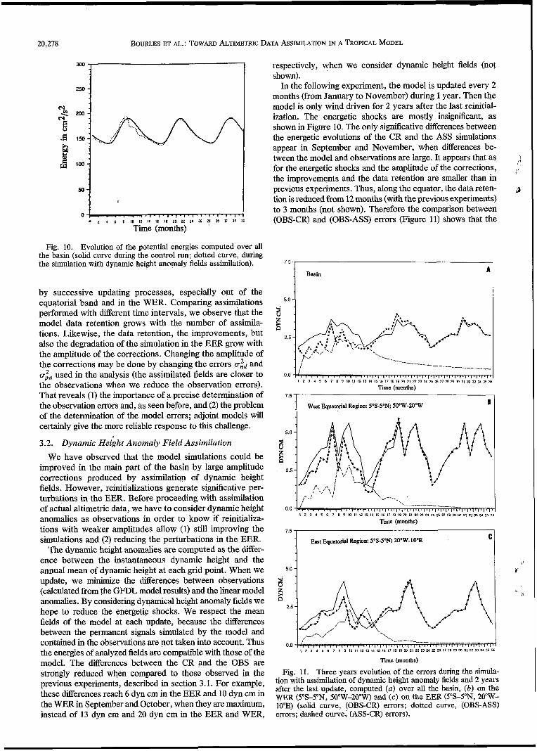
Fig. 10. Evolution of the potential energies computed over all the basin (solid curve during the control run; dotted curve, during the simulation with dynamic height anomaly fields assimilation).

by successive updating processes, especially out of the equatorial band and in the WER. Comparing assimilations performed with different time intervals, we observe that the model data retention grows with the number of assimilations. Likewise, the data retention, the improvements, but also the degradation of the simulation in the EER grow with the amplitude of the corrections. Changing the amplitude of the corrections may be done by changing the errors a,$ and crin used in the analysis (the assimilated fields are closer to the observations when we reduce the observation errors). That reveals (1) the importance of a precise determination of the observation errors and, as seen before, and (2) the problem of the determination of the model errors; adjoint models will certainly give the more reliable response to this challenge.

3.2. Dynamic H&ht Anomaly Field Assimilation We have observed that the model simulations could be

improved in the main part of the basin by large amplitude corrections produced by assimilation of dynamic height fields. However, reinitializations generate significative perturbations in the EER. Before proceeding with assimilation of actual altimetric data, we have to consider dynamic height anomalies as observations in order to know if reinitializations with weaker amplitudes allow (1) still improving the simulations and (2) reducing the perturbations in the EER.

The dynamic height anomalies are computed as the difference between the instantaneous dynamic height and the annual mean of dynamic height at each grid point. When we update, we minimize the differences between observations (calculated from the GFDL model results) and the linear model anomalies. By considering dynamical height anomaly fields we hope to reduce the energetic shocks. We respect the mean fields of the model at each update, because the differences between the permanent signals simulated by the model and contained in the observations are not taken into account. Thus the energies of analyzed fields are compatible with those of the model. The differences between the CR and the OBS are strongly reduced when compared to those observed in the previous experiments, described in section 3.1. For example, these differences reach 6 dyn cm in the EER and 10 dyn cm in the WER in September and October, when they are maximum, instead of 13 dyn cm and 20 dyn cm in the EER and WER,

respectively, when we consider dynamic height fields (not shown).

In the following experiment, the model is updated every 2 months (from January to November) during 1 year. Then the model is only wind driven for 2 years after the last reinitialization. The energetic shocks are mostly insignificant, as shown in Figure 10. The only significative differences between the energetic evolutions of the CR and the ASS simulations appear in September and November, when daerences between the model and observations are large. It appears that as for the energetic shocks and the amplitude of the corrections, the improvements and the data retention are smaller than in previous experiments. Thus, along the equator, the data retention is reduced from 12 months (with the previous experiments) to 3 months (not shown). Therefore the comparison between (OBS-CR) and (OBS-ASS) errors (Figure 11) shows that the

7 5 I

Basin

5.0

A

I 2 3 4 5 6 7 8 9 IO 11 12 I3 11 15 16 II 18 1'2 x ) 13 22 23 24 25 26 21 28 29 30 31 32 33 Y I36

Time (months) 75

West Equatorial Region: 5'S-5"N, 5ooW-2OoW Il

I i..;

0.0 , ', , , , , , ., 1 2 3 4 5 6 7 6 Q IO Il 12 13 14 15 16 I7 I S 19 ?t 21 22 23 24 25 26 27 26 29 30 31 32 33 Y 35 36

Time (months)

5.0 1 I

0.0 1 2 3 4 5 6 7 B Q IO I l 12 I2 14 I5 16 17 I8 IS 20 21 22 23 24 25 26 27 ls 2p 31 32 33 24 35 36

Time (months)

Fig. 11. Three years evolution of the errors during the simulation with assimilation of dynamic height anomaly fields and 2 years after the last update, computed (a) over all the basin, ( b ) on the WER (5"%5"N, 5OoW-2O0W) and (c ) on the EER (YS-YN, 20"W- 10"E) (solid curve, (OBS-CR) errors; dotted curve, (OBS-ASS) errors; dashed curve, (ASS-CR) errors).


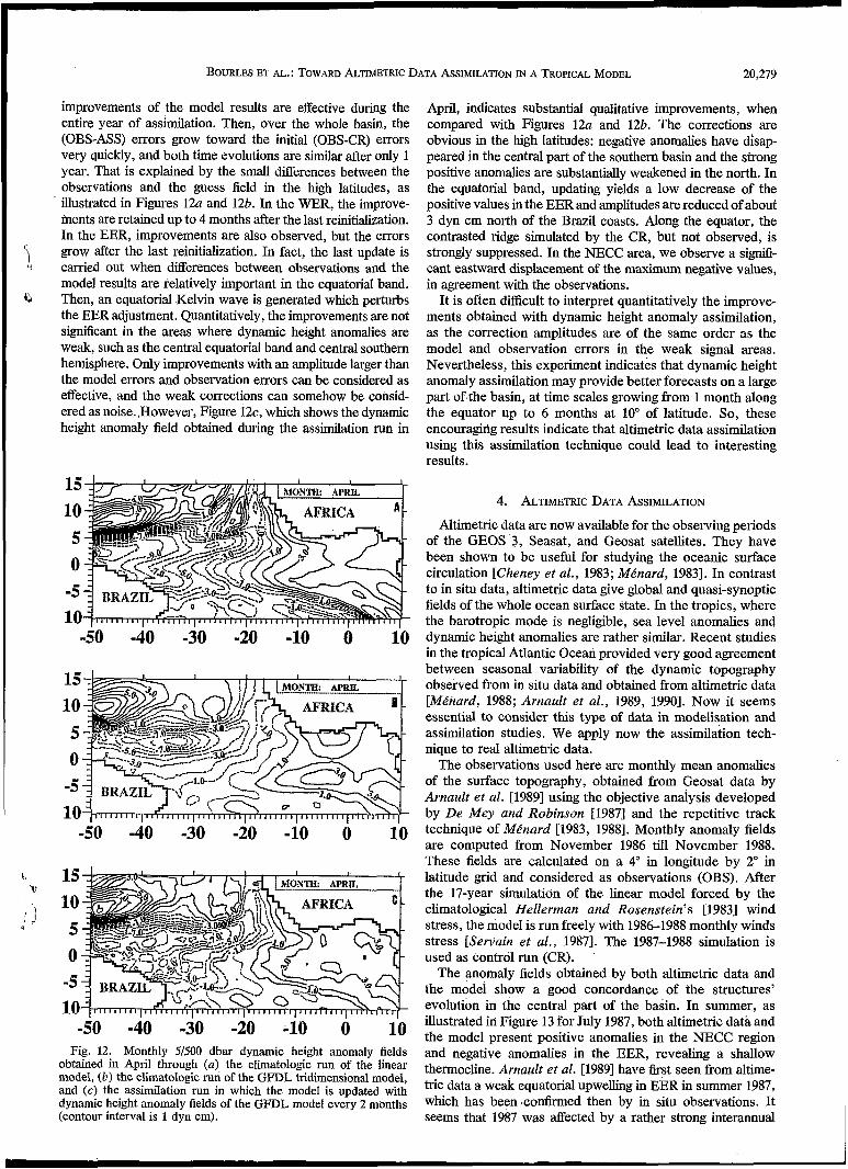
improvements of the model results are effective during the entire year of assimilation. Then, over the whole basin, the (OBS-ASS) errors grow toward the initial (OBS-CR) errors very quickly, and both time evolutions are similar after only 1 year. That is explained by the small differences between the observations and the guess field in the high latitudes, as illustrated in Figures 12a and 12b. In the WER, the improvements are retained up to 4 months after the last reinitialization. In the EER, improvements are also observed, but the errors grow after the last reinitialization. In fact, the last update is carried out when differences between observations and the model results are relatively important in the equatorial band. Then, an equatorial Kelvin wave is generated which perturbs the EER adjustment. Quantitatively, the improvements are not significant in the areas where dynamic height anomalies are weak, such as the central equatorial band and central southem hemisphere. Only improvements with an amplitude larger than the model errors and observation errors can be considered as effective, and the weak corrections can somehow be considered as noise. ,However, Figure 1212, which shows the dynamic height anomaly field obtained during the assimilation run in

15 10 5 O

-5 10

-50 -40 -30 -20 -10 O ¡O

-50 -40 -30 -20 -10 O 10

15 10 5 O

-5 10

-50 -40 -30 -io -io o i o Fig. 12. Monthly 5600 dbar dynamic height anomaly fields

obtained in April through (a) the climatologic run of the linear model, (b ) the climatologic run of the GFDL tridimensional model, and (c) the assimilation run in which the model is updated with dynamic height anomaly fields of the GFDL model every 2 months (contour interval is 1 dyn cm).

April, indicates substantial qualitative improvements, when compared with Figures 12a and 12b. The corrections are obvious in the high latitudes: negative anomalies have disappeared in the central part of the southern basin and the strong positive anomalies are substantially weakened in the north. In the equatorial band, updating yields a low decrease of the positive values in the EER and amplitudes are reduced of about 3 dyn cm north of the Brazil coasts. Along the equator, the contrasted ridge simulated by the CR, but not observed, is strongly suppressed. In the NECC area, we observe a significant eastward displacement of the maximum negative values, in agreement with the observations.

It is often difficult to interpret quantitatively the improvements obtained with dynamic height anomaly assimilation, as the correction amplitudes are of the same order as the model and observation errors in the weak signal areas. Nevertheless, this experiment indicates that dynamic height anomaly assimilation may provide better forecasts on a large part of.the basin, at time scales growing from 1 month along the equator up to 6 months at 10" of latitude. So, these encouragirig results indicate that altimetric data assimilation using this assimilation technique could lead to interesting results.

4. ALTIMETRIC DATA ASSIMILATION

Altimetric data are now available for the observing periods of the GEOS 3, Seasat, and Geosat satellites. They have been shown to be useful for studying the oceanic surface circulation [Cheney et al., 1983; Ménurd, 19831. In contrast to in situ data, altimetric data give global and quasi-synoptic fields of the whole ocean surface state. In the tropics, where the barotropic mode is negligible, sea level anomalies and dynamic height anomalies are rather similar. Recent studies in the tropical Atlantic Ocean provided very good agreement between seasonal variability of the dynamic topography observed from in situ data and obtained from altimetric data [Ménard, 1988; Arnuult et al., 1989, 19901. Now it seems essential to consider this type of data in modelisation and assimilation studies. We apply now the assimilation technique to real altimetric data.

The observations used here are monthly mean anomalies of the surface topography, obtained from Geosat data by Arnault et al. [1989] using the objective analysis developed by De Mey and Robinson [1987] and the repetitive track technique of Ménard [1983, 19881. Monthly anomaly fields are computed from November 1986 till November 1988. These fields are calculated on a 4" in longitude by 2" in latitude grid and considered as observations (OBS). After the 17-year simulation of the linear model forced by the climatological Hellerman and Rosenstein's [ 19831 wind stress, the model is run freely with 1986-1988 monthly winds stress [Servain et al . , 19871. The 1987-1988 simulation is used as control run (CR).

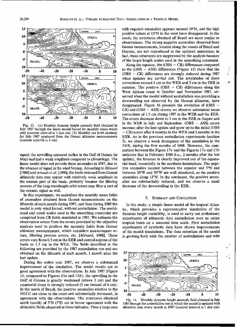
The anomaly fields obtained by both altimetric data and the model show a good concordance of the structures' evolution in the central part of the basin. In summer, as illustrated in Figure 13 €or July 1987, both altimetric data and the model present positive anomalies in the NECC region and negative anomalies in the EER, revealing a shallow thermocline. Arnuult et al. [1989] have first seen from altimetric data a weak equatorial upwelling in EER in summer 1987, which has been'confirmed then by in situ observations. It seems that 1987 was affected by a rather strong interannual


-50 -40 -30 -20 -io ò i o

-50 -40 -30 -20 -10 i i o Fig. 13. (u) Monthly dynamic height anomaly field obtained in

July 1987 through the linear model forced by monthly mean winds only (contour interval is 1 dyn cm). (b) Monthly sea level anomaly for July 1987 produced from the Geosat altimeter measurements (contour interval is 1 cm).

signal; the upwelling appeared earlier in the Gulf of Guinea (in May) and had a weak amplitude compared to climatology. The linear model does not provide these anomalies in 1987, due to the absence of signal in the wind forcing. According to Ménard [1988] andArnault et al. [1990], the fields obtainedfrom Geosat altimetric data may appear with relatively weak amplitude in the eastern part of the basin, probably because the filtering process of the long-wavelength orbit errors may filter a part of the oceanic signal as well.

In this experiment, we assimilate the monthly mean fields of anomalies obtained from Geosat measurements on the fifteenth of each month during 1987, and then during 1988 the model is only wind forced, without assimilation. The meridional and zonal scales used in the smoothing constraint are computed from CR fields simulated in 1987. We estimate the observation errors from the errors provided by the objective analysis used to produce the anomaly fields from Geosat altimeter measurements, which considers measurement errors, filtering process errors, etc. [Mé'nard, 19881. These errors vary from 0.5 cm in the EER and central regions of the basin to 1.5 cm in the WER. The fields described in the following are provided by the 1987 assimilation run and are obtained on the fifteenth of each month, 1 month after the last update.

During the entire year 1987, we observe a substantial improvement of the simulation. The model results are in good agreement with the observations. In July 1987 (Figure 14, compared to Figures 13a and 13b), the upwelling in the Gulf of Guinea is greatly weakened (above 3 cm) and the equatorial slope is strongly reduced (3 cm instead of 6 cm). In the north of Brazil, the positive anomalies relative to the NECC are close to the coast and substantially increased, in agreement with the observations. The structures obtained north (south) of 5"N (5%) are in better agreement with the altimetric fields observed at these latitudes. Thus a large area

with negative anomalies appears around 10"N, and the high positive values at 10"N in the west have disappeared. In the south, the structures obtained off Brazil are more similar to observations. The strong negative anomalies observed from Geosat measurements, located along the coasts of Brazil and Guyana, are not reproduced in the updated simulation; in fact, these structures are suppressed by the analysis because of the larger length scales used in the smoothing constraint.

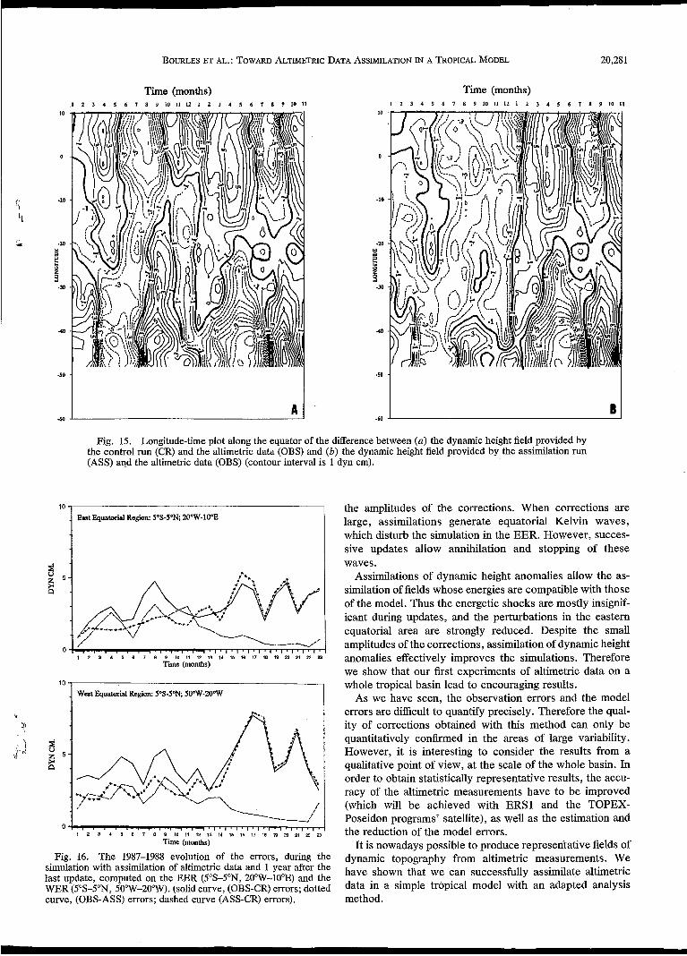
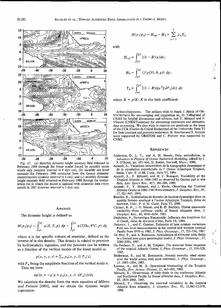
Along the equator, the (OBS - CR) differences compared to the (OBS - ASS) differences (Figure 15) show that the (OBS - CR) differences are strongly reduced during 1987 when updates are carried out. The amplitudes of these corrections exceed 4 cm in the WER and 3 cm in the EER in summer. The positive (OBS - CR) differences along the West African coast in October and November 1987, observed when the model without assimilation was providing a downwelling not observed by the Geosat altimeter, have disappeared. Figure 16 presents the evolution of (OBS - CR) and (OBS - ASS) errors; we observe substantial mean corrections of 1.5 cm during 1987 in the WER and the EER. The errors decrease down to 3 cm in the EER in August and in the WER in July and September. (OBS - ASS) errors increase after the last update and grow up to the initial (OBS - CR) errors after 6 months in the WER and 3 months in the EER. As in the previous assimilation experiments (section 3), we observe a weak divergence of the simulation in the EER, during the first months of 1988. However, the comparison between the Figure 17c and the Figures 17a and 17b indicates that in February 1988 (i.e., 2 months after the last update), the forecast is clearly improved out of the equatorial band, essentially in the northern hemisphere. The negative anomalies located between the equator and SON and between 20"W and 50"W are well simulated, as the positive anomalies along 12"N. In the southeast, the positive anomalies are substantially reduced, and we observe a small decrease of the downwelling in the EER.

5. SUMMARY AND CONCLUSION

In this study, a simple linear model of the tropical Atlan- tic, which provides a representative simulation of the dynamic height variability, is used to carry out preliminary experiments of altimetric data assimilation over an entire tropical basin on a seasonal time scale. First assimilation experiments of synthetic data have shown improvements of the model simulations. The data retention of the model is growing both with the number of assimilations and with

-30 -40 -30 -20 -io ò i o Fig. 14. Monthly dynamic height anomaly field obtained in July

1987 through the assimilation run in which the model is updated with altimetric data every month in 1987 (contour interval is 1 dyn cm).

BOURLES ET AL.: TOWARD ALTIMETRIC DATA ASSIMILATION IN A TROPICAL MODEL 20.281

Time (months) l Z 3 4 5 6 1 8 Y 1 0 1 1 1 1 1 1 J 4 S 6 7 8 9 ~ O ~ l

Time (months) 1 2 1 4 5 6 7 B 9 1 0 1 1 L 1 i 1 3 4 5 6 7 1 9 1 0 1 1

10

O

-10

.10 Y

6 : .M

-tu

-50

.a , -.I I) Fig. 15. Longitude-time plot along the equator of the difference between (u) the dynamic height field provided by

the control run (CR) and the altimetric data (OBS) and (b) the dynamic height field provided by the assimilation run (ASS) and the altimetric data (OBS) (contour interval is 1 dyn cm).

CI

O 1 2 3 4 6 8 7 U 9 IO 11 I2 13 14 I5 16 I7 18 18 20 21 22 P

Time (months)

West Equptorial Region: 5OS-YN 5O0W-2O"W I

o : , , , . . , , , , , . , . , , , , , . I , , , , . * I 1 2 3 4 6 8 1 8 U IO Il 12 13 I4 15 16 17 I8 10 20 21 22 P

Time (months)

Fig. 16. The 1987-1988 evolution of the errors, during the simulation with assimilation of altimetric data and 1 year after the last update, computed on the EER (5"S-5"N, 20"W-10"E) and the WER (YS-YN, 5O0W-20"W). (solid curve, (OBS-CR) errors; dotted curve, (OBS-ASS) errors; dashed curve (ASS-CR) errors).

the amplitudes of the corrections. When corrections are large, assimilations generate equatorial Kelvin waves, which disturb the simulation in the EER. However, successive updates allow annihilation and stopping of these waves.

Assimilations of dynamic height anomalies allow the assimilation of fields whose energies are compatible with those of the model. Thus the energetic shocks are mostly insignificant during updates, and the perturbations in the eastern equatorial area are strongly reduced. Despite the small amplitudes of the corrections, assimilation of dynamic height anomalies effectively improves the simulations. Therefore we show that our first experiments of altimetric data on a whole tropical basin lead to encouraging results.

As we have seen, the observation errors and the model errors are dacul t to quantify precisely. Therefore the qual- ity of corrections obtained with this method can only be quantitatively confirmed in the areas of large variability. However, it is interesting to consider the results from a qualitative point of view, at the scale of the whole basin. In order to obtain statistically representative results, the accuracy of the altimetric measurements have to be improved (which will be achieved with ERS1 and the TOPEX- Poseidon programs' satellite), as well as the estimation and the reduction of the model errors.

It is nowadays possible to produce represen'tative fields of dynamic topography from altimetric measurements. We have shown that we can successfully assimilate altimetric data in a simple tropical model with an adapted analysis method.


15

10

5

O

-5

10 o 10 -10 -20 -40 -30 -50

-30 -20 -io o i o -40 -50

-50 -40 -30 -20 -io o 10 Fig. 17. (a) Monthly dynamic height anomaly field obtained in

February 1988 through the linear model forced by monthly mean winds only (contour interval is 1 dyn cm), ( b ) monthly sea level anomaly for February 1988 produced from the Geosat altimeter measurements (contour interval is 1 cm), and ( c ) monthly dynamic height anomaly field obtained in February 1988 through the assimilation run in which the model is updated with altimetric data every month in 1987 (contour interval is 1 dyn cm).

APPENDIX

The dynamic height is defined as

H(P1lP2) = Il2 a(S, T , p ) d p - llz (Y(35%o,0°c,p) dp

where (Y is the specific volume of seawater, defined as the inverse of in situ density. This density is related to pressure by hydrostaticity equation, and the pressure can be written as a function of the vertical modes of the linear model as

P(Xl Y 3 z , t ) = 1, P n b , Y 3 t ) F A Z )

with F n being the amplitude function of the vertical mode n. Thus we have

dp/az = -p 'g = P , ~ ( X , Y , t ) dF,(z) /dz

We calculate the density from the state equation of Millero and Poisson [1981], and we obtain the dynamic height expression

3

n = 1

with

Y , = Ilz [(l - R)/gp21(dF,/dz) dp

where R = p / K ; K is the bulk coefficient.

Acknowledgnzents. The authors wish to thank J. Merle of OR- STOM/Paris for encouraging and supporting us, O. Tallagrand of CNRS for helpful discussions and advices, and Y. MBnard and P. Vincent (CNES/Toulouse) for interesting comments and altimetric data processing. We also wish to express our gratitude to the team of the CCR (Centre de Calcul Recherche) of the University Paris VI for their constant and precious assistance. B. Bourles and S. Arnault were supported by ORSTOM and C. Provost was supported by CNRS .

REFERENCES Anderson, D. L. T., and A. M. Moore, Data assimilation, in

Advances in Physics of Ocean Numerical Modeling, edited by J. J. O'Brien, pp. 437-464, D. Reidel, Norwell, Mass., 1986.

Amault, S., Variations saisonnières de la topographie dynamique et de la circulation superficielle de 1' Océan Atlantique Tropical, thèse, Univ. P. et M. Curie, Paris VI, 1984.

Amault, S., Y. Ménard, and M. C. Rouquet, Variability of the Tropical Atlantic in 19861987 as observed by Geosat and in situ data, Adv. Space Res., 9(7), 383-386, 1989.

Amault, S . , Y. MBnard, and J. Merle, Observing the Tropical Atlantic Ocean in 19861987 from altimetry, J . Geophys. Res., 95,

Bourlès, B., Assimilation de donnees de hauteur dynamique dans un modèle linéaire appliqué 9 l'océan Atlantique Tropical, thèse de doctorat, Univ. P. et M. Curie, Paris VI, 1990.

Cheney, R. E., J. G. Marsh, and B. D. Beckley, Global mesoscale variability from collinear tracks of Seasat altimeter data, J . Geophys. Res., 88, 4343-4354, 1983.

Delécluse, P., Dynamique Equatoriale: Influence des frontières Est et Ouest, thèse de doctorat d'état, Paris VI, 1984.

Delcroix, T., and C. Gautier, Estimates of heat content variations from sea level measurements in the central and western tropical Pacific from 1979 to 1985, J . Phys. Oceanogr., 17,725-734, 1987.

De Mey, P., and A. Robinson, Assimilation of altimeter eddy fields in a limited area quasi-geostrophic model, J . Phys. Oceanogr., 17, 2280-2293, 1987.

Du Penhoat, Y., and A. M. Tréguier, The seasonal linear response of the tropical Atlantic Ocean, J . Phys. Oceunogr., 15, 316-329, 1985.

Hellerman, S., and M. Rosenstein, Normal monthly wind stress over the world ocean with error estimates, J . Phys. Oceunogr.,

17, 921-945, 1990.

13, 1093-1104, i983. Leetma, A., and M. Ji, Operational hindcasting of the Tropical

Pacific, Dyn. Atnzos. Oceans, 13, 465-490, 1989. MBnard, Y., Observation of eddy fields in the northwest Atlantic

and Northwest Pacific by Seasat altimeter data, J . Geophys. Res.,

Ménard, Y . , Observing the seasonal variability in the tropical Atlantic from altimetry, J . Geophys. Res., 93, 13,967-13,978, 1988. '

88, 1853-1866, 1983.


Merle, J., and H. Gillet, Les crises climatiques, in Encyclopaedia Universalis, pp. 152-157, Paris, 1985.

Miller, L., R. E. Cheney, and D. Milbert, Sea level time series in the equatorial Pacific from satellite altimetry, Geopltys. Res. Lett., 13, 375-478, 1986.

Millero, F., and A. Poisson, International one atmosphere equation of state of seawater, Deep Sea Res., 28A, 525-529, 1981.

Moore, A. M., Aspect of geostrophic adjustement during tropical ocean data assimilation, J . Plzys. Oceanogr., 19, 435-461, 1989.

Moore, A. M., and D. L. T. Anderson, The assimilation of XBT data into a layer model of the tropical Pacific ocean, Dyn. Atinos.

Moore, A. M., N. S. Cooper, and D. L. T. Anderson, Initialisation and data assimilation in models of the Indian ocean, J . Pltys. Oceanogr., 17, 1965-1977, 1987.

MorliBre, A., G. Reverdin, and J. Merle, Assimilation of temperature profiles in a oceanic general circulation model for a continu- ous survey of tropical Atlantic, J . Pltys. Oceartogr., 19, 1892-

Philander, R. G. H., and R. C. Pacanowski, Simulation of the seasonal cycle in the tropical Atlantic Ocean, Geopltys. Res. Lett., 13, 802-804, 1984.

Philander, R. G. H., and R. C. Pacanowski, A model of a seasonal cycle in the tropical Atlantic, J . Geophys. Res., 91, 14,192- 14,206, 1986.

Philander, R. G. H., S. G. H. Hurlin, and R. C. Pacanowski, Initial

1 Oceans, 13, 441-464, 1989. -5

1899, 1989. *

conditions for a general model of tropical oceans, J. Phys. Oceanogr., 17, 147-157, 1987.

Provost, C., A variational method for estimating the general circulation in the ocean, Ph.D. thesis, Univ. of Calif., San Diego, 1983.

Provost, C., and R. Salmon, A variational method for inverting hydrographic data, J . Mar. Res., 44, 1-34, 1986.

Sasaki, Y., Some basic formalisms in numerical variational analysis, Mon. Weather Rev., 98, 875-883, 1970.

Servain, J., M. Serva, S. Lukas, and G. Rougier, Climatic atlas of the tropical Atlantic wind stress and sea surface temperature 1980-1984, Ocean Air Interactions, I , 109-182, 1987.

Sheibaum, J., and D. L. T. Anderson, Variational assimilation of XBT data, part 2, Sensitivity studies and use of smoothing constraints, J . Plzys. Oceanogr., 20, 689-704, 1990.

S. Amault, Laboratoire d'Océanographie Dynamique et de Cli- matologie, ORSTOM, Université Paris VI, 4 place Jussieu, T14-2, 75252 Paris Cedex 05, France.

B. Bourles, Centre ORSTOM de Cayenne, BP 165, 97323 Cay- enne Cedex, French Guiana.

C. Provost, Laboratoire d’océanographie Dynamique et de Cli- matologie, CNRS, Université Paris VI, 4 place Jussieu, T14-2,75252 Paris Cedex 05, France.

(Received August 5, 1991; revised April 15, 1992;

accepted May 22, 1992.)

c Y I

Documents

Toward altimetric data assimilation in a Tropical Atlantic ...horizon.documentation.ird.fr/exl-doc/pleins_textes/pleins_textes_6/... · JOURNAL OF GEOPHYSICAL RESEARCH, VOL. 97, NO