Embed Size (px)
Citation preview
Toward a unified global regulatory
capital framework for life insurers
by
Ishmael Sharara
A thesis
presented to the University of Waterloo
in fulfillment of the
thesis requirement for the degree of
Doctor of Philosophy
in
Actuarial Science
Waterloo, Ontario, Canada, 2010
c⃝ Ishmael Sharara 2010

I hereby declare that I am the sole author of this thesis. This is a true copy of the
thesis, including any required final revisions, as accepted by my examiners.
I understand that my thesis may be made electronically available to the public.
ii
Abstract
In many regions of the world, the solvency regulation of insurers is becoming
more principle-based and market oriented. However, the exact forms of the solvency
standards that are emerging in individual jurisdictions are not entirely consistent. A
common risk and capital framework can level the global playing field and possibly
reduce the cost of capital for insurers. In the thesis, a conceptual framework for
measuring the insolvency risk of life insurance companies will be proposed. The
two main advantages of the proposed solvency framework are that it addresses the
issue of incentives in the calibration of the capital requirements and it also provides
an associated decomposition of the insurer’s insolvency risk by term. The proposed
term structure of insolvency risk is an efficient risk summary that should be readily
accessible to both regulators and policyholders. Given the inherent complexity of the
long-term guarantees and options of typical life insurance policies, the term structure
of insolvency risk is able to provide stakeholders with more complete information
than that provided by a single number that relates to a specific period. The capital
standards for life insurers that are currently existing or have been proposed in Canada,
U.S., and in the EU are then reviewed within the risk and capital measurement
framework of the proposed standard to identify potential shortcomings.
iii

Acknowledgements
I would like to thank my supervisors, Prof Mary Hardy and Prof David Saunders,
for the help and support that they provided to me during a very challenging time.
I also want to acknowledge the other members of the PhD committee: Thanks to
Prof Rob Brown for making those long trips to attend the defenses! Prof Hyuntae
Kim for challenging me to look deeper into my work and Prof James Thompson for
the interesting read, it was worthwhile! I also want to thank Dr. Allen Brender for
making himself available and for the helpful comments that he provided.
Last but not least, I want to say a special thanks to Mary Lou Dufton who helped
me in numerous ways throughout the course of my program.
iv

Dedication
Ecclesiastes 9:11
I returned, and saw under the sun, that the race [is] not to the swift, nor the battle
to the strong, neither yet bread to the wise, nor yet riches to men of understanding,
nor yet favour to men of skill; but time and chance happeneth to them all.
I dedicate this thesis to God and my young family. Thank you all for being very
patient and fair with me.
v
Table of Contents
List of Tables x
List of Figures xi
1 Introduction 1
1.1 Background . . . . . . . . . . . . . . . . . . . . . . . . . . . . . . . . 1
1.1.1 Overview . . . . . . . . . . . . . . . . . . . . . . . . . . . . . 1
1.1.2 U.S. Risk Based Capital . . . . . . . . . . . . . . . . . . . . . 3
1.1.3 Canadian MCCSR . . . . . . . . . . . . . . . . . . . . . . . . 4
1.1.4 Solvency II . . . . . . . . . . . . . . . . . . . . . . . . . . . . 5
1.2 Thesis motivation . . . . . . . . . . . . . . . . . . . . . . . . . . . . . 8
1.2.1 Why regulate life insurers? . . . . . . . . . . . . . . . . . . . . 8
1.2.2 The measurement problem of ruin theory . . . . . . . . . . . . 10
1.3 Accomplishments of thesis . . . . . . . . . . . . . . . . . . . . . . . . 18
1.4 Outline of thesis . . . . . . . . . . . . . . . . . . . . . . . . . . . . . . 21
2 A conceptual framework for a unifying global capital standard 22
2.1 Introduction . . . . . . . . . . . . . . . . . . . . . . . . . . . . . . . . 22
2.2 An asset-liability model for a life insurer . . . . . . . . . . . . . . . . 23
vi

2.2.1 Model definition . . . . . . . . . . . . . . . . . . . . . . . . . . 23
2.2.2 Market value of assets and liabilities . . . . . . . . . . . . . . 24
2.2.3 Solvency capital rules . . . . . . . . . . . . . . . . . . . . . . . 26
2.2.4 Term structure of insolvency risk . . . . . . . . . . . . . . . . 27
2.2.5 Framework for policyholder-oriented risk management incentives 29
2.3 Outline of the proposed regulatory capital framework . . . . . . . . . 30
2.3.1 GFAs for asset and liability valuation . . . . . . . . . . . . . . 32
2.3.2 GFAs for regulatory capital . . . . . . . . . . . . . . . . . . . 37
3 A review of the MCCSR, US RBC and Solvency II formulas 50
3.1 Overview . . . . . . . . . . . . . . . . . . . . . . . . . . . . . . . . . . 50
3.2 A benchmark review of the standard formulas . . . . . . . . . . . . . 53
3.2.1 Definition of terms . . . . . . . . . . . . . . . . . . . . . . . . 53
3.2.2 Market-valuation based balance sheet . . . . . . . . . . . . . . 55
3.2.3 Capital requirements . . . . . . . . . . . . . . . . . . . . . . . 62
3.3 Chapter conclusion . . . . . . . . . . . . . . . . . . . . . . . . . . . . 68
4 Proposal of an ALM risk measurement framework 69
4.1 Overview . . . . . . . . . . . . . . . . . . . . . . . . . . . . . . . . . . 69
4.1.1 Motivation . . . . . . . . . . . . . . . . . . . . . . . . . . . . . 69
4.1.2 Outline of chapter . . . . . . . . . . . . . . . . . . . . . . . . 71
4.2 Model insurer . . . . . . . . . . . . . . . . . . . . . . . . . . . . . . . 72
4.2.1 Model insurance portfolio . . . . . . . . . . . . . . . . . . . . 72
4.2.2 Assumed investment strategies of the model insurer . . . . . . 73
4.3 Definitions of supervisory target capital . . . . . . . . . . . . . . . . . 76
4.4 A numerical comparison of the proposed ALM risk capital requirements 80
vii
4.4.1 Sample distribution of supervisory target capital . . . . . . . . 80
4.4.2 Insolvency risk profile implied by supervisory target capital . 83
4.4.3 What risk is being measured? . . . . . . . . . . . . . . . . . . 87
4.4.4 Term structure of ALM risk . . . . . . . . . . . . . . . . . . . 91
4.4.5 An incentive-based review of proposed capital standards . . . 106
4.5 The impact of model risk on relative risk and capital assessments . . 109
4.6 Chapter conclusion . . . . . . . . . . . . . . . . . . . . . . . . . . . . 113
5 Policy recommendations and future research 116
5.1 Introduction . . . . . . . . . . . . . . . . . . . . . . . . . . . . . . . . 116
5.2 Market discipline . . . . . . . . . . . . . . . . . . . . . . . . . . . . . 117
5.3 Proposed Canadian and Solvency II capital standards . . . . . . . . . 119
5.4 US PBA capital standard . . . . . . . . . . . . . . . . . . . . . . . . 120
5.5 Other potential applications of thesis results . . . . . . . . . . . . . . 121
5.6 Conclusion and future research . . . . . . . . . . . . . . . . . . . . . 121
Appendices 125
A Data and formulas for Chapter 3 calculations 125
A.1 Model portfolio and valuation assumptions . . . . . . . . . . . . . . . 125
A.2 MCCSR formula . . . . . . . . . . . . . . . . . . . . . . . . . . . . . 126
A.3 U.S. RBC formula . . . . . . . . . . . . . . . . . . . . . . . . . . . . 130
A.4 Solvency II standard formula . . . . . . . . . . . . . . . . . . . . . . . 132
B Assumptions for Chapter 4 calculations 138
B.1 Mortality table assumption . . . . . . . . . . . . . . . . . . . . . . . . 138
B.2 Initial interest rates . . . . . . . . . . . . . . . . . . . . . . . . . . . . 138
viii

B.3 The C-3 phase III interest rate generator: model specification . . . . 141
B.4 Simulated sample key interest rates from the C3 Phase III generator . 142
Bibliography 144
ix
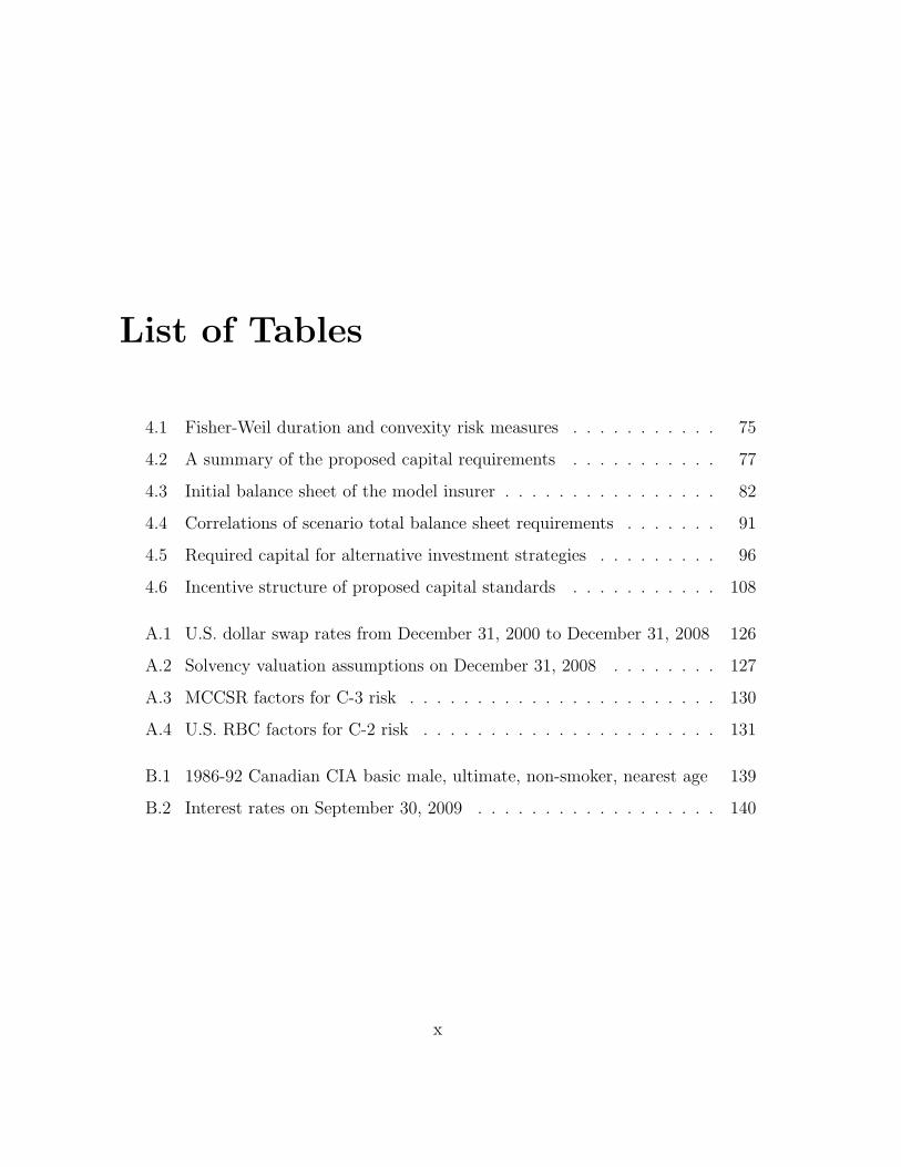
List of Tables
4.1 Fisher-Weil duration and convexity risk measures . . . . . . . . . . . 75
4.2 A summary of the proposed capital requirements . . . . . . . . . . . 77
4.3 Initial balance sheet of the model insurer . . . . . . . . . . . . . . . . 82
4.4 Correlations of scenario total balance sheet requirements . . . . . . . 91
4.5 Required capital for alternative investment strategies . . . . . . . . . 96
4.6 Incentive structure of proposed capital standards . . . . . . . . . . . 108
A.1 U.S. dollar swap rates from December 31, 2000 to December 31, 2008 126
A.2 Solvency valuation assumptions on December 31, 2008 . . . . . . . . 127
A.3 MCCSR factors for C-3 risk . . . . . . . . . . . . . . . . . . . . . . . 130
A.4 U.S. RBC factors for C-2 risk . . . . . . . . . . . . . . . . . . . . . . 131
B.1 1986-92 Canadian CIA basic male, ultimate, non-smoker, nearest age 139
B.2 Interest rates on September 30, 2009 . . . . . . . . . . . . . . . . . . 140
x

List of Figures
3.1 Total balance sheet requirements . . . . . . . . . . . . . . . . . . . . 57
3.2 Free capital of the model insurer . . . . . . . . . . . . . . . . . . . . . 58
4.1 Scenario Total Balance Sheet Requirements . . . . . . . . . . . . . . 81
4.2 Insolvency risk profile implied by supervisory target capital . . . . . . 84
4.3 Incremental capital charge for balance sheet solvency . . . . . . . . . 86
4.4 Risky scenario set for U.S. PBA . . . . . . . . . . . . . . . . . . . . . 88
4.5 Risky scenario set for Solvency II . . . . . . . . . . . . . . . . . . . . 89
4.6 Measured risk exposure of investment strategies . . . . . . . . . . . . 94
4.7 Measured risk exposure of investment strategies (cont’d) . . . . . . . 95
4.8 Tail-dependencies of alternative measures of (long-bond) ALM risk . . 100
4.9 Tail-dependencies of alternative measures of (short-bond) ALM risk . 101
4.10 Marginal risk contributions of the long-bond strategy by period . . . 104
4.11 Marginal risk contributions of the short-bond strategy by period . . . 105
4.12 Reinvestment risk of the short bond strategy . . . . . . . . . . . . . . 111
B.1 C3 Phase III scenarios: sample key rates . . . . . . . . . . . . . . . . 143
xi

Chapter 1
Introduction
1.1 Background
1.1.1 Overview
The subject matter pertaining to the solvency regulation of financial institutions has
become very topical in recent years. The changes to the solvency regulation of finan-
cial institutions that are occurring globally are in response to factors such as the need
to level the global playing field, the increase in complexity of products, the globaliza-
tion of insurance and financial capital markets, and the need to prevent regulatory
arbitrage across sectors of the financial industry. Additionally, the recent global fi-
nancial crisis has proven to be a significant catalyst for advancing the crucial debate
on the regulation of financial institutions, especially those deemed to be systemically
important.
The Basel Committee on Banking Supervision (BCBS) which effectively sets
global prudential bank standards issued the first Basel capital accord in 1988 (BIS
1

(1988)). To date, there have been two further iterations of the original accord (BIS
(2006, 2010)) to address perceived shortcomings in the global bank capital rules. The
International Association of Insurance Supervisors (IAIS) and International Actuar-
ial Association (IAA) have done considerable work on developing a global standard
for insurer solvency assessment (e.g. Sandstrom (2006); IAIS (2002, 2005, 2007);
IAA (2004)). The International Accounting Standards Board (IASB) and U.S. Fi-
nancial Accounting Standards Board (FASB) are collaborating to develop a single
global standard for insurance contracts. This collaboration has recently resulted in
the issuance of an exposure draft of the proposed International Financial Reporting
Standard (IFRS) for insurance in July 2010. The main elements of the proposed
insurance accounting standard are summarized in IASB (2010). In contrast to the
accounting model that was described in the previously issued discussion paper (IASB
(2007)), the exposure draft values insurance contracts using a fulfilment cost method
rather than exit value. Insurance liabilities that are outlined in the exposure draft
include deferred amounts of profit that result from a calibration to premium at in-
ception. The measured contract liability is therefore not economic. The final IFRS
for insurance is not expected to be issued until June 2011. The importance of having
harmonized insurance accounting bases for public financial and regulatory reports is
noted in IAA (2004).
Individual jurisdictions have also undertaken projects to modernize their solvency
standards for insurers. Brief descriptions of the developments that are occurring in
the U.S., Canada and EU are provided next.
2
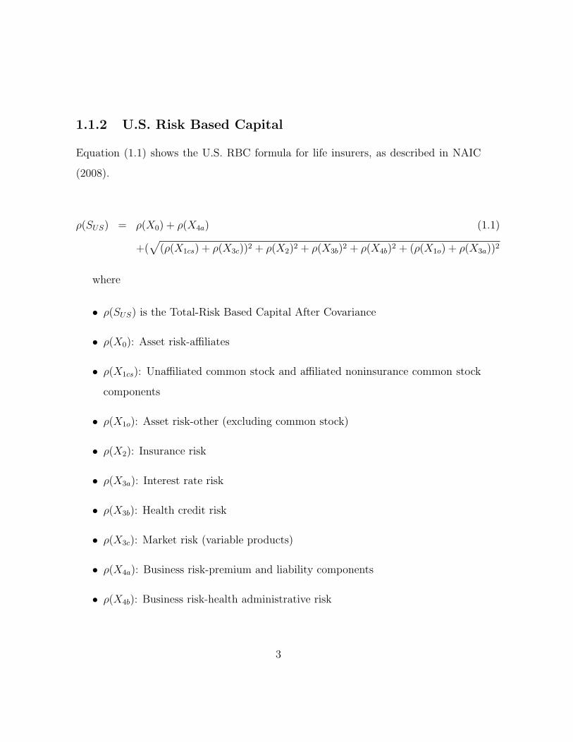
1.1.2 U.S. Risk Based Capital
Equation (1.1) shows the U.S. RBC formula for life insurers, as described in NAIC
(2008).
ρ(SUS) = ρ(X0) + ρ(X4a) (1.1)
+(√
(ρ(X1cs) + ρ(X3c))2 + ρ(X2)2 + ρ(X3b)2 + ρ(X4b)2 + (ρ(X1o) + ρ(X3a))2
where
• ρ(SUS) is the Total-Risk Based Capital After Covariance
• ρ(X0): Asset risk-affiliates
• ρ(X1cs): Unaffiliated common stock and affiliated noninsurance common stock
components
• ρ(X1o): Asset risk-other (excluding common stock)
• ρ(X2): Insurance risk
• ρ(X3a): Interest rate risk
• ρ(X3b): Health credit risk
• ρ(X3c): Market risk (variable products)
• ρ(X4a): Business risk-premium and liability components
• ρ(X4b): Business risk-health administrative risk
3
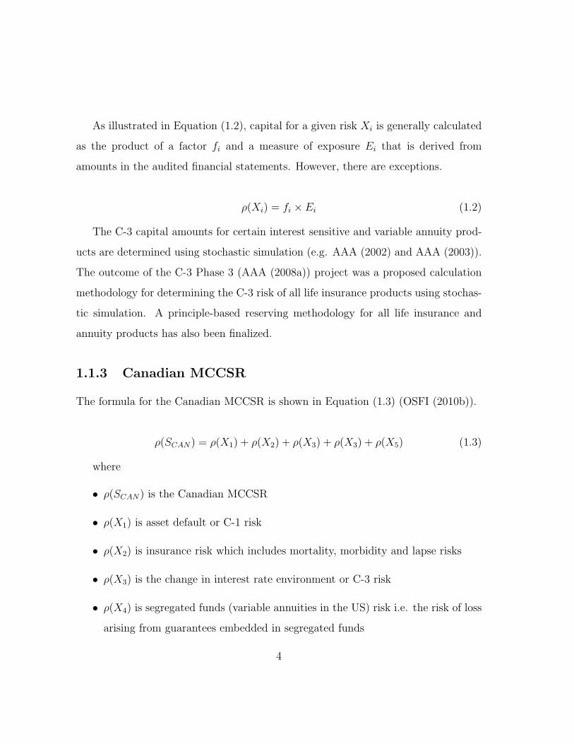
As illustrated in Equation (1.2), capital for a given risk Xi is generally calculated
as the product of a factor fi and a measure of exposure Ei that is derived from
amounts in the audited financial statements. However, there are exceptions.
ρ(Xi) = fi × Ei (1.2)
The C-3 capital amounts for certain interest sensitive and variable annuity prod-
ucts are determined using stochastic simulation (e.g. AAA (2002) and AAA (2003)).
The outcome of the C-3 Phase 3 (AAA (2008a)) project was a proposed calculation
methodology for determining the C-3 risk of all life insurance products using stochas-
tic simulation. A principle-based reserving methodology for all life insurance and
annuity products has also been finalized.
1.1.3 Canadian MCCSR
The formula for the Canadian MCCSR is shown in Equation (1.3) (OSFI (2010b)).
ρ(SCAN) = ρ(X1) + ρ(X2) + ρ(X3) + ρ(X3) + ρ(X5) (1.3)
where
• ρ(SCAN) is the Canadian MCCSR
• ρ(X1) is asset default or C-1 risk
• ρ(X2) is insurance risk which includes mortality, morbidity and lapse risks
• ρ(X3) is the change in interest rate environment or C-3 risk
• ρ(X4) is segregated funds (variable annuities in the US) risk i.e. the risk of loss
arising from guarantees embedded in segregated funds
4

• ρ(X5) is foreign exchange risk
Capital amounts for individual risks are simply summed to get the total amount.
There is therefore no recognition of diversification among the risk classes that underly
the MCCSR formula since the risks are effectively assumed to be perfectly correlated.
As in the case of U.S. RBC, capital for individual risks is generally determined as
the product of a factor and a measure of exposure that is obtained from the annual
financial statement. However, the amount of capital with respect to segregated funds
risk can be determined using internal models (OSFI (2010b)).
All public insurers in Canada have started to report under IFRS as of January 1,
2011. With the expected finalization of Phase 2 of the insurance accounting project
in June 2011, preparations are underway for the adoption of the new standard. Since
regulatory reports are based on public financial reports in Canada, the adoption of
IFRS requires that changes be made to the current MCCSR framework in anticipa-
tion of the new insurance accounting standard. There are also other reasons why the
Office of the Superintendent of Financial Institutions (OSFI) has been reviewing its
capital adequacy framework for life insurers. Among these are the increase in actu-
arial and risk management expertise allowing more sophisticated methods to be used
and the need to consider changes that are currently occurring in other jurisdictions
(JCOAA (2008a)). Background information on the proposed internal model frame-
work is summarized in Table 4.2 of Chapter 4. For more detailed information, refer
to JCOAA (2008a,b); MAC (2007), for example.
1.1.4 Solvency II
Solvency II is the new solvency standard that will apply to insurers that operate in the
European Union. A comprehensive history of the evolution of Solvency II is provided
5
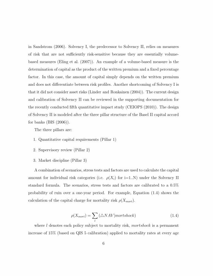
in Sandstrom (2006). Solvency I, the predecessor to Solvency II, relies on measures
of risk that are not sufficiently risk-sensitive because they are essentially volume-
based measures (Eling et al. (2007)). An example of a volume-based measure is the
determination of capital as the product of the written premium and a fixed percentage
factor. In this case, the amount of capital simply depends on the written premium
and does not differentiate between risk profiles. Another shortcoming of Solvency I is
that it did not consider asset risks (Linder and Ronkainen (2004)). The current design
and calibration of Solvency II can be reviewed in the supporting documentation for
the recently conducted fifth quantitative impact study (CEIOPS (2010)). The design
of Solvency II is modeled after the three pillar structure of the Basel II capital accord
for banks (BIS (2006)).
The three pillars are:
1. Quantitative capital requirements (Pillar 1)
2. Supervisory review (Pillar 2)
3. Market discipline (Pillar 3)
A combination of scenarios, stress tests and factors are used to calculate the capital
amount for individual risk categories (i.e. ρ(Xi) for i=1..N) under the Solvency II
standard formula. The scenarios, stress tests and factors are calibrated to a 0.5%
probability of ruin over a one-year period. For example, Equation (1.4) shows the
calculation of the capital charge for mortality risk ρ(Xmort).
ρ(Xmort) =∑l
(NAV |mortshock) (1.4)
where l denotes each policy subject to mortality risk, mortshock is a permanent
increase of 15% (based on QIS 5 calibration) applied to mortality rates at every age
6
and NAV is the change in the insurer’s net asset value (i.e. assets minus liabilities)
given the mortality shock.
The capital amounts for individual risks that have been determined under the
Solvency II standard formula are typically aggregated using Equation (1.10).
ρ(SEU) =
√∑i
∑j
ϕ(i, j) · ρ(Xi) · ρ(Xj) (1.5)
where
• ρ(Xi) is the solvency capital requirement for risk i.
• ϕ(i, j) denotes the (tail) correlation between risks i and j.
A given insurer can calculate its required capital amount using a standard formula,
partial internal model or fully internal model. Under the internal model approach,
an insurer can use an internal model to determine the capital requirement subject
to specific calibration standards in addition to a “use test”. The second pillar of the
Solvency II framework is the means by which the regulator promotes good governance
and risk management practices of the insurer. Under the third pillar, the insurance
supervisor encourages the provision of timely and relevant information on the insurer’s
operations to market participants so that they can monitor the insurer effectively. The
design of Solvency II is also very similar to that of the Swiss Solvency Test (SST)
(see Sandstrom (2006)). In particular, they both determine capital by applying an
appropriately calibrated shock to a risk factor and measuring the impact on the net
assets of the insurer using a market-valuation balance sheet. The notable differences
between the SST and Solvency II include the SST’s use of scenarios to model abnormal
losses.
7
1.2 Thesis motivation
In many regions of the world, the solvency regulation of insurers is becoming more
principle-based and market oriented. However, the exact nature of the solvency stan-
dards that are emerging in individual jurisdictions are not entirely consistent, as
has been suggested above in the case of the U.S. RBC, MCCSR and Solvency II. A
common risk and capital framework can level the global playing field and possibly
reduce the cost of capital for insurers. As has been noted in the introduction, the
IAIS and IAA have done a lot of work in developing a global framework for insurer
solvency assessment. For example, see IAA (2004); IAIS (2002, 2005, 2007). To date,
they have outlined principles for a global capital framework and issued standards and
guidelines to promote the goal of convergence in insurer solvency assessment among
their members.
The primary goal of this thesis is to propose an insolvency risk and capital mea-
surement framework that can be used as benchmark standard for life insurers. The
arguments that will be used to justify the proposed framework will go beyond the
typical considerations of actuarial ruin-theory. As such, the proposed risk and capital
measurement framework should be relatively more robust.
1.2.1 Why regulate life insurers?
Unlike in banking, the failure of an insurer would generally not result in a conta-
gion effect across the industry. According to Cummins et al. (1993), solvency regu-
lation (for insurers) should be designed to duplicate as closely as possible the out-
come of a competitive market in which all parties have access to all relevant infor-
mation. In particular, solvency regulation should address the agency problem that
8
is created by the information asymmetry between the firm owners and policyhold-
ers/debtholders. This is necessary since policyholders are “...dispersed and insuffi-
ciently informed; none of them (individually) has enough incentive to spend time,
energy, and/or financial resources in monitoring the management of her insurance
company” (Plantine and Rochet (2007)). Accordingly, Plantine and Rochet (2007)
suggest a “banker model” of insurance regulation in which the regulator’s role is
limited to the effective representation of the policyholders in the corporate gover-
nance structure of the insurer. Consistent with the banker model of regulation, Doff
(2008) also states that “..the focus of an insurance supervision framework should be
to decrease information asymmetries and to align incentives for policyholders and the
insurance company”.
The following factors tend to make life insurers especially prone to insolvency risk:
1. Insurers generally have ample liquidity even in times of financial distress since
they typically receive premiums well in advance of having to pay claims to poli-
cyholders. The liquidity risk profile of life insurers also differs from that of banks
since life insurance and annuity contracts tend to be long-term, and penalties
and/or other fees are usually assessed for early withdrawal or cancelation of the
policies. The availability of ample liquidity means an insurer is able to con-
tinue in business even if it is losing money as long as its management is able
to conceal current losses in the income statement by understating reserves for
example. The result is that troubled insurers will usually come to the attention
of the regulators and the market when the likely losses for policyholders are
severe (Plantine and Rochet (2007)).
2. Life insurance products generally have long-term guarantees and options that
are difficult to assess in terms of risk. The notable collapse of Equitable Life in
9
the UK was partly due to inadequately priced options in the pension annuity
portfolio (e.g. IAA (2004)). In Eling (2010), insurance business model and
product complexity are suggested as possible reasons why market participants
are not able to effectively monitor the insurer’s risk taking.
Based on the preceding discussion, solvency regulation is essentially required since
the acquisition of information (e.g. assessment of willingness and ability to pay claims
of insurer) by policyholders is costly (e.g. Eling et al. (2007); Cummins et al. (1993)).
As a means to mitigate the information asymmetry between the firm owners and
policyholders, a very accessible and efficient risk summary for life insurers will be
proposed in the thesis.
The disadvantages of stringent solvency regulation include unintended conse-
quences such as unnecessarily high insurance prices and the squeezing out of small
insurers from the market (e.g. Eling et al. (2007); Cummins et al. (1993)).
1.2.2 The measurement problem of ruin theory
In general, the notion that risk can be measured accurately can incentivise manage-
ment to engage in risky behaviour that is not properly accounted for under the capital
standard either because it is too difficult to assess, or because of model error.
Ruin-theory based capital requirements are determined such that they limit the
probability of insurer failure to some very low level that is acceptable to the super-
visor. For an introduction and overview of ruin-theory, see Klugman et al. (1998).
The existing and proposed capital standards for life insurers all tend to be based
on ruin-theory (e.g. MCCSR, US RBC, and Solvency II). However, there are sig-
nificant implementation challenges associated with a ruin-theoretic capital adequacy
framework. Plantine and Rochet (2007) discuss several practical and conceptual lim-
10
itations of ruin-theory. From a theoretical standpoint, the failure of ruin-theory to
account for the response of the market to capital requirements is a particularly no-
table limitation that they cited. They also note that the results of several studies (e.g.
Cummins et al. (1995)) suggest that RBC type formulas are not good predictors of
insurer failure. The computational challenges of ruin theory will be further discussed
in the next sections.
In IAA (2004), the International Actuarial Association (IAA) endorsed the three
pillar structure of Basel II for insurance solvency supervision. The three pillar struc-
ture was discussed in Section 1.1 in the context of Solvency II. Within the three
pillar solvency regulation framework, the pillar 1 capital requirements are viewed as
a buffer to protect against residual risks that were not adequately dealt with under
pillars 2 and 3. For this reason, capital requirements are termed the “last line of
defence” in IAA (2004). Accordingly, we can describe the measurement of pillar 1
capital requirements within a three pillar framework by Equation (1.6).
ρp1(X) = ρ(X)−∆ρp2(X)−∆ρp3(X) (1.6)
where ρ(X) is the appropriate capital amount in the absence of any pillar 2 and
pillar 3 risk mitigating effects i.e. ∆ρp2(X) and ∆ρp3(X) respectively. ρp1(X) is the
pillar 1 capital requirement with respect to residual risks only i.e. after considering
the risk mitigating effects of pillar 2 and pillar 3.
Given the qualitative and/or subjective nature of pillars 2 and 3, the measurement
problem of ruin theory can only be compounded within a three pillar regime.
Eling (2010) defines market discipline in the context of insurance as “the ability
of customers, investors, and intermediaries to monitor and influence the manage-
ment of insurance companies”. The results in Eling (2010) suggest that the extent
11

of market discipline in life insurance is very limited. One reason for the ineffective-
ness of market-discipline is due to the complexity of the products that are offered
by life insurers which makes them very difficult to understand by stake holders. Ad-
ditionally, from the viewpoint of prudential regulation, it is worthwhile to ask to
what extent the market-discipline that can be expected to exist in a given insurance
market is “policyholder-oriented”. That is, does the market-discipline properly re-
flect the regulator’s goal of protecting policyholders? The significant impediments
to policyholder-oriented market discipline that exist in life insurance imply that the
effectiveness of the third pillar is probably very limited. For reasons already men-
tioned, it is likely that the ability of policyholder discipline to be effective will remain
hampered even in the presence of increased disclosures by life insurers.
Pillar 2 is the supervisory effort in promoting good corporate governance and risk
management practices (e.g. stress testing, asset-liability management) by the insurer.
The inclusion of corporate governance and risk management in a solvency regulation
framework was a key recommendation of the “Sharma report” (Sharma (2002)). Un-
der pillar 2, larger insurers are likely to be using economic capital models and sophisti-
cated ERM systems to manage their risk. Generally speaking, insurers using internal
models to determine regulatory capital would be required to ensure consistency with
their economic capital models. The recent global financial crisis showed that the so-
phisticated ERM systems that had been built by the banks were inadequate. The
supervisor needs to be confident that the models being used are appropriate from
the legislated viewpoint of safeguarding the policyholders’ interest. The verification
problem of internal economic capital models led Plantine and Rochet (2007) to not
advocate their use in the determination of regulatory capital. Eling et al. (2007) cite
the possibility of “model arbitrage” as another disadvantage of using internal models
12

for regulatory capital purposes. In fact, based on their overall analysis, including
review of available literature on solvency, Eling et al. (2007) conclude that risk-based
capital models should only be used as guidelines rather than strict requirements since
they have limited predictive utility.
Further, the extent to which the regulator is able to provide effective monitoring
in the design and application of the insurer’s complex risk management models is
questionable at best. The global financial crisis revealed that even rating agencies,
who are paid to provide similar monitoring, were not able to properly assess the risk
of securities in which financial institutions had an interest. Given that the problem
of insurer insolvency is really about bad (and or dishonest) management in many
situations, and the information asymmetry that generally exists between regulators
and the company’s management, the potential rewards of the regulator’s effort under
pillar 2 can be limited.
In conclusion, the accurate application of Equation (1.6) can be seen to be an
extremely challenging endeavour.
Quantitative capital requirements (Pillar 1)
To further our understanding of the challenges involved in the implementation of a
ruin-theory based capital framework, lets consider the following example. Assume
that a given insurer is faced with individual risk exposures Xi for i=1,..,N. For ex-
ample, i could be either of market, credit, insurance or operational risks. Assume
further that each
Xi = µi(1 + Ziνi) (1.7)
where µi is the mean, νi = σi
µiis the coefficient of variation of Xi and Zi is the
standardized random variable corresponding to Xi. The total risk exposure of the
13

insurer is then given by
S = X1 +X2 + ..+XN =N∑i=1
µi(1 + Ziνi) (1.8)
To define a capital requirement based on the given insurer’s risk profile, an appropriate
risk measure must be specified.
A risk measure is defined as any mapping from a random variable to the real
number line, Jorion (2005). The purpose of a risk measure is to summarise the
entire risk distribution X by one number ρ(X). Examples of popular risk measures
include the standard deviation principle, Value at Risk (VaR) and Conditional Tail
Expectation (Tail VaR). Desirable properties of a risk measure for capital adequacy
will be explored in Chapter 2. The overall capital requirement for the given insurer
can be expressed as:
ρ(S) = µS(1 + κSνS) (1.9)
where µS =∑N
i=1 µi, σS = σ(∑N
i=1Xi), νS = σS
µSis the coefficient of variation of S and
κS is a parameter that depends on the compound distribution S and the solvency
standard. For example, if the regulatory solvency standard is calibrated to a 1%
probability of ruin and S is normally distributed, then κS = Φ−1(0.99) where Φ−1 is
the inverse standard normal cumulative distribution function.
Standardized solvency models
The U.S. RBC, Canadian MCCSR, and the Solvency II standard formulas have
been discussed in previous sections. Under the Canadian MCCSR or U.S. RBC for-
mula, capital for a given risk Xi is generally calculated as the product of a factor
and a measure of exposure that is derived from audited financial statements as shown
14
in Equation (1.2). For example, the MCCSR capital buffer for the default risk of
$100 million of AA-rated bonds is calculated by substituting Ei=$100 million and
fi=0.5% (i.e. the 2010 MCCSR factor). By definition, the calibration of a stan-
dardized solvency model (e.g. factors fi in Equation (1.2)) is conservative since it
is meant to cover the tail-risk profile of insurers that operate in a given market or
industry. In a heterogenous insurance market, the conservative calibration of the stan-
dard model implies that it will not accurately portray the economic risk exposures
of a given insurer, especially one that is on the lower-end of the risk-profile spec-
trum. Additionally, volume-based risk measures such as those derived, for example,
by multiplying premium volume by a fixed factor provide misaligned incentives for
prudent risk management. If inappropriate incentives are to be avoided, an insurer’s
regulatory capital should not deviate significantly from its economic capital.
The U.S. RBC, Canadian MCCSR and Solvency II standard formulas use dif-
ferent aggregation techniques to approximate the overall capital requirement of the
insurer ρ(S) from the capital requirements of the individual risk categories (ρ(Xi)
for i=1..N). The U.S. RBC capital amounts are aggregated using Equation (1.1) (see
NAIC (2008)). Equation (1.1) effectively assumes correlations of either 0 or 1 between
categories of risk. On the other hand, the capital requirements for individual risk
categories under the Canadian MCCSR are aggregated using Equation (1.3) (OSFI
(2008)). By simply summing up the capital requirements for individual risks, the
Canadian MCCSR effectively assumes that the risks Xi are perfectly correlated. The
prescribed correlation matrix approach that is used under the Solvency II standard
formula to combine risks at each aggregation level is summarized by Equation (1.10)
(for example, see CEIOPS (2010)). The calibration of the correlations ϕ(i, j) is such
that they produce an overall capital requirement ρ(SEU) at the 99.5% confidence level
15
over a one year period. Equation (1.10) can be shown to produce correct results in
the case of linear correlations only when the underlying distributions Xi are elliptical
e.g. multivariate normal. However, many loss distributions in insurance are skewed,
as are credit, market and operational risks.
ρ(SEU) =
√∑i
∑j
ϕ(i, j) · ρ(Xi) · ρ(Xj) (1.10)
where
• ρ(Xi) is the solvency capital requirement for risk i.
• ϕ(i, j) denotes the (tail) correlation between risks i and j.
The US RBC, MCCSR and the Solvency II standard formulas use different ap-
proaches to combine risks. This is a reflection of the inherent difficulty in modelling
dependency.
Internal solvency models
The solvency regulation of insurers in many jurisdictions is moving toward more
principle-based regimes for reasons cited in the introductory paragraph. In particular,
insurers are for the first time being given the opportunity to use internal models
to determine regulatory capital, generally subject to specific calibration standards
and a “use test”. The idea of using an institution’s internal model for determining
regulatory capital was introduced in a 1996 market-risk amendment to the Basel
II accord (BIS (1996)). An internal model framework allows a better alignment
of a financial institution’s regulatory capital with economic capital by giving the
16
institution more control over the definition and calibration of the parameters of the
regulatory capital model. In Hardy (1993) a compelling argument for the use of
stochastic modeling in life insurer solvency assessment was presented. In the analysis
that was conducted, both relative and absolute solvency risk assessments of several
life offices with different risk profiles were shown to be potentially misleading when
they are conducted using deterministic scenarios rather than stochastic scenarios.
For example, an insurer might use the method of copulas to model the dependen-
cies among the risk categories Xi rather than a simpler approach underlying a given
solvency standard.
Definition 1. Embrechts et al. (2001)
An N-dimensional copula is a function C with domain [0, 1]N such that
1. C is grounded and n-increasing.
2. C has margins Ck, k=1,..,N, which satisfy Ck(u) = u for all u in [0,1].
Copulas are a useful alternative to linear correlation in dependency modeling since
they can be chosen and calibrated to more accurately capture the assumed joint tail-
behavior of the risk factors, which could be very different from their behaviour under
normal situations. Sklar’s Theorem (see Embrechts et al. (2001)) as restated below
demonstrates the usefulness of the copula concept in risk management.
Theorem 1. (Sklar’s Theorem) Let H be an N-dimensional distribution function
with margins F1,...,FN . Then there exists an N-copula C such that for all x in RN ,
H(x1, . . . , xN) = C(F1(x1), . . . , FN(xN)).
If F1,...,FN are all continuous, then C is unique; otherwise C is uniquely deter-
mined on Ran F1,...,Ran FN . Conversely, if C is an N-copula and F1,...,FN are
17
distribution functions, then the function H defined above is an N-dimensional distri-
bution function with margins F1,...,FN .
Using the technique of copulas, the joint distribution of the component risks H(X1,
. . . , XN) which is required to calculate ρ(S), is modeled by separately specify-
ing the distribution of the marginals (Fi, i=1,..N) and the dependence structure, as
represented by the copula C. An example of a copula that can be used to derive
multivariate distributions from the modeled univariate distributions Fi, i=1,..,N is
the N-dimensional Gaussian copula Cθ given by
Cθ(F1(x1), ..., FN(xN)) = Φθ(Φ−1(F1(x1)), ...,Φ
−1(FN(xN)))
where Φθ is the multivariate standard normal distribution with correlation matrix
θ and Φ−1 is the inverse of Φ, the standard normal distribution function.
There are other risk management tools that can afford the insurer an opportunity
to enhance the accuracy of the regulatory capital calculations performed using a
fully-internal model. For example, Extreme Value Theory (EVT) can be very useful
in approximating the tail-losses that are important for calculating regulatory capital.
McNeil et al. (2005) contains a comprehensive discourse on EVT and its applications.
1.3 Accomplishments of thesis
The practical implementation challenges of a ruin-theory based capital framework
have been discussed in the preceding sections. Plantine and Rochet (2007) considered
the shortcomings of ruin theory significant enough to abandon the theory altogether in
favor of an alternative theory that is based on corporate finance arguments. Starting
with the perfect capital market assumptions of Modigliani and Miller (1958) and
18
then introducing agency risk into the analysis, they conclude that the potential role
of capital in a solvency regulatory framework is in its use as an incentive device for
aligning the interests of shareholders and policyholders. The impact of capital on
shareholder risk-taking behavior is then likened to the effect of a deductible on an
insurance policyholder.
In this thesis, a different approach is taken from that of Plantine and Rochet
(2007). The framework for insurer capital requirements that is developed in the thesis
combines both the incentive and ruin-theoretic roles of capital, rather than completely
discarding ruin-theory altogether. The two key insights of Plantine and Rochet (2007)
that are retained in the proposed framework are the following:
1. Capital can be used as incentive device to mitigate moral hazard risk, as ex-
plained by the deductible analogy.
2. The role of the solvency/prudential regulator is limited to the aggressive repre-
sentation of the policyholders in the management of the insurer since policyhold-
ers typically do not have representation in the corporate governance structure
of insurers.
The problem with using pillar 2 as the main instrument of solvency supervision is
that it is qualitative and very subjective by nature. It is hard to legislate “desired”
behaviour. However, it is possible to promote sound policyholder-oriented risk man-
agement policies by the insurer through the use of carefully designed and calibrated
incentives. In the recommended framework, capital has a dual role. It is a buffer
against residual risks and also a robust mechanism of incentives for sound risk be-
haviour by shareholders. The incentive effect reinforces the pillar 2 supervisory effort.
It can be argued that the more important of the two roles of capital is the one in which
19
it is regarded as a system of incentives. Given the important and powerful role of
incentives in driving risk management behaviour, a capital framework that considers
incentives as an input rather than an output of the model should be superior.
The main accomplishments of the thesis are the following:
1. A unified framework for analyzing insurer insolvency risk and capital is pro-
posed. Additionally, a term structure decomposition of the insurer’s insolvency
risk is proposed to assist in the insolvency risk analysis. By providing an ad-
ditional (time) dimension to insolvency risk measurement, the term structure
decomposition provides a more complete picture of the insurer’s overall insol-
vency risk compared to traditional capital standards that only provide a single
number to summarize the insurer’s total exposure. For example, a term struc-
ture decomposition of an insurer’s insolvency risk might reveal that a one-year
based capital requirement is grossly misleading as a measure of the insurer’s
time-dependent risk exposure.
2. The unified capital framework is also applied to the measurement of ALM risk
for life insurers. The proposed ALM risk and capital framework is “policyholder-
oriented”, defined in this thesis to mean capital requirements or corresponding
incentives that are completely aligned with the overall goal of prudential regu-
lation.
3. The unified capital framework and its associated term structure decomposition
can be applied to enhance the effectiveness of all three-pillars of the solvency
regulation framework.
4. The term structure decomposition of insolvency or ALM risk can be used in
other applications as well. For example, it can be used to provide more complete
20
risk information to the stakeholders of an insurer in public financial reports. It
can also be potentially used in portfolio optimization and economic capital
calculations.
1.4 Outline of thesis
The context of the current thesis engagement has been provided in this chapter. In
Chapter 2, the proposed benchmark global capital framework will be outlined. A
method to decompose the capital or risk that has been calculated within the frame-
work of the benchmark standard will also be presented in this chapter. In Chapter
3, the effectiveness of the existing Canadian MCCSR and US RBC standards, and
the Solvency II standard formula, will be compared against the benchmark capital
standard that is proposed in Chapter 2. In particular, special attention will be paid
to the incentives that are provided under these standardized capital frameworks to
assess whether they are “policyholder-oriented”. The unified global framework for
measuring ALM risk and capital is presented in 4. Finally, Chapter 5 concludes by
offering policy recommendations regarding the Solvency II, US PBA, and Canadian
capital standards. Suggestions for future research are also listed in that final chapter.
21
Chapter 2
A conceptual framework for a
unifying global capital standard
2.1 Introduction
In this chapter, a conceptual framework for a unifying global standard will be pro-
posed. The two main advantages of the proposed solvency framework are that it
addresses the issue of incentives in the calibration of the capital requirements and it
also provides an associated decomposition of the insurer’s insolvency risk by term.
When the incentive effect of capital is considered, pillar 1 of the three pillar solvency
framework is no longer just a buffer to absorb residual risks. Rather, the incentives
that are created by the capital requirements can facilitate the qualitative and subjec-
tive efforts of the supervisor under the remaining pillars. According to Cummins et al.
(1993), solvency regulation should be designed to duplicate as closely as possible the
outcome of a competitive market in which all parties have access to all relevant infor-
mation. The proposed term structure of insolvency risk is an efficient summary of the
22

insurer’s risk information that should be readily accessible to all market participants,
including regulators and policyholders. Given the inherent complexity of the long-
term guarantees and options of typical life insurance policies, the term structure of
insolvency risk is able to provide stakeholders with more complete information than
that provided by a single number that relates to a specific period.
A solvency model for a life insurer will now be presented in the context of asset-
liability mismatch risk as a means to introduce notation and solvency concepts that
will be used in the remainder of the thesis.
2.2 An asset-liability model for a life insurer
2.2.1 Model definition
The insurance model is a multi-period discrete time model. The solvency risk mea-
surements are based on monte-carlo simulations of many sample paths of the relevant
risk factors (e.g. equity prices, interest rates or commodity futures prices) over the
time horizon T. Denote each simulated sample path by ω ∈ Ω. Suppose that (Ω,F ,P)
is a probability space with filtration Ft; t=1,..,T. P is a real-world or physical
probability measure. Let X(ω) denote the value taken by the random variable X in
the state of the world ω.
We define the following adapted stochastic processes:
• MVAt is the market value of assets of the insurer at time t.
• MVLt is the market value of insurer’s liabilities at time t.
• ALRt= MVAt/MVLt is the assets to liability ratio.
23
• Θ=Θt, t=1,..,T denotes an investment, risk management or trading strategy.
Each Θt is a random vector showing the amount of each security invested in the
asset portfolio at time t.
LCF(ω) = LC1(ω),LC2(ω), ... and ACF(ω) = AC1(ω),AC2(ω), ... are the li-
ability and asset cash flows along the path ω.
2.2.2 Market value of assets and liabilities
In this section, the meaning of market value of insurance liabilities will be explained.
Generally speaking, financial economics principles should be the basis for calculating
the market value of insurance liabilities. Panjer et al. (1998) contains illustrative
applications of financial economics to insurance and pension valuation.
Babbel et al. (2002) examine the specific issues, such as the treatment of default
and liquidity risk, that arise in the application of financial economics principles to
the valuation of illiquid life insurance liabilities. In Black and Scholes (1973); Merton
(1974), a holding in corporate debt can be treated as a combined position in risk-
free debt and a short put. Babbel et al. (2002) illustrate the pricing of a bullet GIC
and whole life insurance product using a similar decomposition technique that dis-
aggregates the insurance liability into a risk-free amount that measures the insurer’s
indebtedness (“Treasury” or “defeasance” value) and a put option amount that re-
flects default risk. Using the notation of the previous section, Equation (2.1) shows
the calculation of this Treasury value for a whole life insurance policy that is exposed
to interest-sensitive surrenders. At t=0, TVL0 is the Treasury value of the liabili-
ties, Er represents risk-neutral expectation with respect to risk-free interest rates r
and Em|r is the conditional expectation with respect to mortality risk given interest
rates. If mortality risk is orthogonal to interest rate risk, mortality can be treated
24
as deterministic in Equation (2.1) (i.e. in the evaluation of the inner expectation
Em|r). A surrender function that summarizes the relationship between interest rates
and surrenders can be postulated and used as the basis for determining the interest-
sensitive component cash flows of LCt for t=1,2,..,T. To price in the ‘default’ put
option POVL0, option-adjusted spreads in respect of non-completely orthogonal and
non-diversifiable (e.g. systematic mortality) risks are applied along the interest rate
paths. Equation (2.2) then shows that the market value of liabilities MVL0 is the
defeasance value minus the value of the put option.
TVL0 = Er(Em|r(T∑t=1
LCte−rt·t)) (2.1)
MVL0 = TVL0 − POVL0 (2.2)
The valuation of insurance liabilities in this manner is consistent with the market-
based valuations of interest-rate derivative securities which require the specifica-
tion and calibration of an arbitrage-free model for the short rate r. For example,
Hull and White (1993) compare different approaches to developing arbitrage-free term
structure models and describe a numerical procedure for constructing a variety of
single-factor models.
A comprehensive review of the pricing, reserving and capital assessment techniques
of equity-linked life insurance contracts from both the actuarial and dynamic hedging
perspectives can be found in Hardy (2003). Option-pricing techniques for valuing in-
surance are also illustrated in Boyle and Hardy (1997, 2007). Bader and Gold (2003)
support the application of financial economics principles to the valuation of defined
pension plans for regulatory solvency and public reporting purposes. In particular,
they argue against the use of book valuation methods, and the traditional actuar-
25
ial practice of using a valuation discount rate that reflects the assumed long-term
investment strategy of the pension plan.
2.2.3 Solvency capital rules
The following definitions of solvency have been used in the actuarial literature.
1. An insurer is solvent at time t if MVAt ≥ Lt. Define this as “point-in-time”
(PIT) solvency.
2. If at time t, MVA(ω)t+1 ≥ MVL(ω)t+1, the insurer is solvent under scenario ω.
Define this as “short-term solvency” (STS). The regulatory capital framework
that was proposed in IAA (2004) is based on the STS perspective. Similarly,
the Solvency II (CEIOPS (2010)), Swiss Solvency Test (Sandstrom (2006)), and
the proposed Canadian capital requirements (OSFI (2010a); MAC (2007)) for
life insurers are also calibrated in this setting.
3. If MVA(ω)t ≥ MVL(ω)t for t=0,1...,n for n=2,..,T-1 where T is the maturity of
liability cash flows, then the insurer meets the “n-year balance sheet solvency”
(XnYR) condition under scenario ω. The short-term solvency (STS) definition
would be equivalent to an X1YR rule but has been separately considered due
to its relevance as indicated in the preceding bullet.
4. We define long-term balance sheet solvency (LTBS) as the situation when
MVAt ≥ MVLt for t=0,1,..,T, where T is the maturity of the liability cash
flows. The determination of principle-based U.S. RBC that is described in
AAA (2008a, 2002, 2003) is based on the LTBS formulation albeit using statu-
tory rather than market values of assets and liabilities.
26
5. Let MVAt+1=MVAt(1 +Rt)− LCFt+1, where Rt is the random t-period invest-
ment return. Define δt=MVAt+1−MVAt. The insurer is solvent in the cash flow
sense (i.e. “cash-flow solvency” (CFS)) if MVA0+∑T−1
t=0 δt ≥ 0. The Canadian
Asset Liability Method (CALM) (ASB (Canada) (2009)) and U.S. principle-
based reserve method are applications of the cash flow solvency concept.
2.2.4 Term structure of insolvency risk
It is useful to consider a method to map out the insolvency risk profile of the insurer
through time t. The insolvency risk term structure would provide similar information
to that provided by a mortality table for a cohort of insureds. Alternatively, it can be
likened to an implied volatility term structure derived from option prices of different
maturities.
Equation (2.3) shows the recursive calculation of the insurer’s assets MVAt(ω) for
t=0,1,..,T-1; given projected liability cashflows LC1(ω),LC2(ω),LC3(ω), ... under
scenario path ω, where Rt(ω) is the investment return and MVA0(ω) is the amount
used as the starting assets in the projection.
MVAt+1(ω) = MVAt(ω)(1 + Rt(ω))− LCFt+1(ω) (2.3)
The projected liability values Lt(ω) for t=0,1,..,T are determined using the appli-
cable valuation basis.
If we require MVAt ≥ Lt for t=0,1...,n, for solvency, we can define the aggregate
loss random variable Sn for a given solvency assessment horizon n=1,2,...,T using
Equation (2.5), where T is the maturity of the liability cashflows.
27
Sn = min∆∈R
MVA0 = (L0 +∆)|ALRt >= 1; t = 0, 1, ..., n (2.4)
= X1 +X2 + ...+Xn (2.5)
where Xt for t=1,..,n is the marginal loss random variable corresponding to time
period t. Equation (2.6) expresses Xt in terms of S(.) (assume S0=0).
Xt = St − St−1 (2.6)
= min∆∈R
MVA0 = (St−1 +∆)|ALRt >= 1 (2.7)
The interpretation of Xt(ω) is that it is the non-negative amount of top-up required
to the assets at time t=0 so that ALRt(ω) >= 1, given that the insurer was solvent
under that scenario path ω to the beginning of the period (i.e. ALRi(ω) >= 1 for all
i=0,1,..,t-1).
Let Ωtail = ω ∈ Ω|ST (ω) > V aRα(ST ) for α in [0,1]. Now taking expectations of
the quantities in Equation (2.5) for n=T, we obtain the insolvency risk decomposition
in Equation (2.8).
E(ST |Ωtail) = E(X1|Ωtail) + E(X2|Ωtail) + ...+ E(XT |Ωtail) (2.8)
The insolvency term structure expressed by Equation (2.8) is a useful construct
since it provides an attribution of the insurer’s default risk (as measured by TVaRα(ST ))
to future periods. It will be used to explain important results in the remainder of the
thesis. Tail-value at risk (TVaR) has been widely used in capital allocation problems
similar to its use in Equation (2.8). For example, Panjer (2001) uses it for allocating
capital to the business lines of a financial conglomerate.
28
2.2.5 Framework for policyholder-oriented risk management
incentives
In this section, notation for explaining the role of policyholder-oriented incentives
in the design and calibration of the proposed model for capital requirements will be
introduced.
Define d(X,Y) to be some measure of distance between the multivariate random
vectors X=(X1,X2,...,XT ) and Y=(Y1,Y2,...,YT ), with means µX , µY and covari-
ance matrices∑
X and∑
Y . Assume that Y is an objective that has to be achieved,
and that X represents the random possible outcomes of a given process that has
been designed to achieve those goals. Then d(X,Y) can been interpreted as a mea-
sure of the risk of the process in achieving the objective. In the present context,
we can assume that Y represents the liability cash flows of the insurer, that is, Y=
LC1,LC2,LC3, .... In our proposed framework, as discussed in previous sections,
the sole objective of the prudential regulator is to safeguard these policyholder obli-
gations. If X represents the corresponding cash flows from the insurer’s assets given
a particular operational, investment or business strategy, we have the interpretation
that d(X,Y) is a measure of the riskiness of the strategy, or of the insurer’s insolvency
risk, in general. We can make the same argument using the market values of assets
and liabilities instead of cash flows.
In order to promote the alignment of the interests of the shareholders with the
regulatory objective, the capital requirements can be defined in manner that creates
appropriate shareholder/managerial incentives for sound policyholder-oriented risk
management (PORM). To better articulate the role of capital as an incentive device in
29

solvency regulation, Equation 2.9 defines an “incentive function” on given regulatory
capital requirements ρ(.).
I(J,K) = ρ(J)− ρ(K) (2.9)
I(J,K) in Equation (2.9) provides a measure of the monetary incentives or reward
for changing the underlying strategy from J to K. If J is a riskier strategy than K,
in terms of the regulatory objective, we should have I(J,K) ≥ 0. If K corresponds to
an insurer strategy that perfectly replicates the liability cash flows, then
I(J,K) = ρ(J)− ρ(K)
= ρ(J) (2.10)
since ρ(K) = 0. That is, the monetary incentive for adopting the minimum-risk
strategy K is the full amount of regulatory capital associated with the current strategy
J. In the special case when the strategy K is the benchmark strategy (i.e. exact proxy
for regulatory objective), we refer to I(J,K) as the PORM incentives of strategy J.
They are policyholder-oriented since they represent the “reward” for moving down
the risk spectrum toward the regulatory objective.
2.3 Outline of the proposed regulatory capital frame-
work
The proposed framework for a unified global capital standard for life insurers is pre-
sented in the following sections. The proposed Global Framework Attributes (GFAs)
will be discussed under two broad categories of a regulatory capital framework:(1)
valuation of assets and liabilities (2) required capital. As has been previously noted,
30
the IAIS has done related work. To date, they have published principles, standards
and guidelines for a solvency assessment framework that they hope will be adopted
by each of the IAIS member states. In that regard, some of the GFAs presented will
be largely consistent with the IAIS principles, outlined in IAIS (2002, 2005, 2007), for
example. In Cummins et al. (1993), seven specific objectives of risk-based capital are
provided. One of these objectives is that the risk-based capital requirements should
provide “incentives” for insurers to reduce insolvency risk.
The distinguishing feature of the work in this thesis is the great emphasis it places
on having appropriate “policyholder-oriented risk management (PORM) incentives”
within a pillar 1 capital framework for reasons previously cited in the thesis. As
discussed in previous sections, the empirical evidence available (e.g. Sharma (2002))
suggests that failure in corporate governance and risk management is frequently the
cause of insurer insolvency, rather than inadequate capital per se. The proposed
GFAs are therefore generally based on the following two important insights:
1. The overriding goal of prudential supervision is limited to the aggressive rep-
resentation of an insurer’s existing policyholders in its corporate governance
structure. In the proposed framework, the prudential regulator does not need
to consider the interests of other stakeholders such as employees and sharehold-
ers of the insurer, similar to the approach of Plantine and Rochet (2007). The
problem of poor corporate governance and risk management that is generally
associated with failed insurers can be expected to be especially pronounced in
a principle-based environment for solvency regulation.
2. The single objective of all three pillars of the solvency framework is to pro-
mote policyholder-oriented corporate governance and risk management by the
insurer’s shareholders/management in a coherent and harmonized manner. In
31
particular, pillar 1 capital requirements should be structured to provide ap-
propriate shareholder/management behavioral incentives to support the second
and third pillars.
2.3.1 GFAs for asset and liability valuation
The GFAs for the valuation of assets and liabilities are largely consistent with the
IAIS principles stated in IAIS (2002, 2005, 2007).
GFA 1
(1.1) The solvency assessment of all assets and liabilities should be
based on fundamental economic values
Fundamental economic values require the use of realistic assumptions and meth-
ods to value assets and liabilities. They do not include arbitrary levels of con-
servatism. A solvency framework benefits from the use of economic values since
they are more objective, transparent and relevant, compared to alternative val-
uation systems. For example, the book valuation of assets and the formulaic-
approach to life insurance reserves under the current U.S. NAIC standard (see
Lombardi (2006)) do not represent assessments of fundamental economic value.
Using an equity-indexed annuity portfolio as an example, Wallace (2006) demon-
strates that the underlying risk of the portfolio is only properly reflected when
economic values (in this example, also market values) for assets and liabilities
are used. When historical accounting or other U.S. GAAP-based valuations are
used, the resulting measured risk can be dangerously misleading.
Further, for the policyholder-oriented incentives defined in Equation (2.9) to
have their intended effect, they must be structured in the context of economic
32
valuations.
(1.2) The valuation of assets and liabilities should be calibrated to
the market, as far as possible.
When the market for an asset or liability is active, transparent and liquid, its
market value should be used as the basis for measuring fundamental economic
value. If there is no ready market for the asset or liability, the estimate of
fundamental economic value should be based on market-inputs that have been
derived from similar or other instruments, provided that this is reasonable. The
added transparency and objectivity of market values allows market participants
and the regulator to make more meaningful assessments of the insurer’s financial
position. Therefore, the solvency monitoring of the insurer that is performed
under pillars 2 and 3 is enhanced when market values are used. The book
valuation of assets and the formula-based life insurance reserves under the U.S.
NAIC system are objective, but they do not properly reflect the risk of the
underlying cash flows. Other advantages of market-based valuation include the
following:
• As stated previously, a major root cause for insurer solvency failures is due
to incompetent or dishonest management. For example, in the situation
when an insurer’s management consistently understates reserves or under-
prices policies, the insolvency risk profile of the insurer takes the character
of a ponzi scheme with an ultimate ruin or default probability of 1. The
objectivity and transparency of market-based valuations helps to mitigate
such operational risks.
• A mark-to-market solvency framework would also be advantageous since
33
the use of fair value or market value in public accounting has generally
increased. The desirability of a harmonized solvency and public reporting
standard is noted in IAA (2004).
Three categories of fair-value measurements are defined under the U.S.
FASB Statement No. 157, Fair Value Measurements (i.e. US GAAP). In
order of reliability, they are: quoted market prices in active markets (level
1), mark-to-model prices (level 2), and the unobservable inputs category
that uses (subjective) estimates and assumptions in the valuation (level
3). The corresponding International Accounting Standard, IAS 39, is very
similar.
The convergence of financial reporting standards to IFRS globally, as noted
in Chapter 1, lends credence to the use of a mark-to-market valuation
framework in the solvency assessment of an insurer. As described in the
exposure draft of the IFRS for insurance IASB (2010), the measured in-
surance contract liability does not reflect a fair or “exit” value estimate.
However, the sum of the first two components (i.e. best estimate lia-
bility plus risk adjustment, from the insurer’s perspective) has a strong
resemblance to fair or market value making it easier to reconcile the two
amounts.
• A mark-to-market (MtM) paradigm for all the assets and liabilities of the
insurer ensures consistency in their valuation for solvency assessment. As
suggested in IAA (2004), an inconsistent valuation of assets and liabilities
would create hidden surplus or deficit.
• Alternative statutory solvency asset valuation approaches such as histor-
ical cost, amortized cost and the equity method do not provide current
34
estimates of value that are risk-sensitive. The disadvantages of using val-
uations that are not market-based will be elaborated later in Chapter 3,
in the context of the statutory valuation practices that are in current use
in Canada and the U.S.. The results of Chapter 3 demonstrate the inap-
propriate incentives that result when non market-based or risk-insensitive
methods are used to value the insurer’s assets and liabilities.
As described in IAA (2004), the collapse of the Equitable Life Assurance Society
in the U.K. was partly a result of inadequately priced guarantees and options
in a portion of their pension portfolio. If market or option pricing theory-
based methods had been used to explicitly reflect the value of these options and
guarantees in a transparent manner, it is possible that the collapse of a such a
major insurer could have been prevented.
Notwithstanding the significant risk management benefits of market valuation,
there are also significant implementation challenges. Examples of the challenges
include:
• Most insurance liabilities are illiquid and will not have a readily available
quoted market price, the most reliable estimate of fair value (Level 1)
under US GAAP, as described above. In the terminology of US FAS 157,
many insurance liabilities would fall under the Level 3 type of fair value,
which is the more subjective and least reliable of the three categories of fair
valuation. Under Solvency II, the challenge of determining an “implied”
or “extrapolated” market value of insurance liabilities was addressed by
prescribing the cost of capital methodology (e.g. CEIOPS (2010)) for
measuring the liability risk margin. As can be expected, a lot of simplifying
35
assumptions were required to make this approach viable within a principle-
based solvency framework. For example, a fixed cost of capital rate is
assumed for all insurers, life and P&C insurers alike. Towers Perrin (2004)
discuss the practical implementation challenges of a fair value approach in
the context of P&C insurers.
• As observed in the recent global financial crisis, liquidity can suddenly dry
up for some markets under stressed conditions. In this case, estimates of
fundamental value are made using the less reliable level-3 type of valuation,
for example.
• Procyclical capital requirements are those that tend to exacerbate prevail-
ing market conditions. Risk-sensitive market valuations are more prone to
procyclicality, in comparison to book valuation methods for example.
(1.3) The calculation of the policyholder liability should provide sep-
arate estimates for the best estimate liability and solvency margin
Separate estimates of the best estimate liability and solvency margin enable
effective absolute and relative assessments of insurer financial strength. Knowl-
edge of the best estimate liability would allow stakeholders of the insurer to
make informed judgements of the actual levels of capitalization. Hirst et al.
(2007) also note how market participants feel more confident about the quality
of an earnings forecast when information on the source of the earnings by line
item is also included in the disclosure. Therefore, the effectiveness of market
discipline can be potentially enhanced when market participants receive disag-
gregated risk information on the liabilities since they are more confident to act
on that information.
36
2.3.2 GFAs for regulatory capital
GFA 2
(2.1) The global capital framework must be principle-based
(2.2) The regulatory capital requirements should be calibrated to an
overall enterprise level of statistical confidence
The capital requirement should be principle-based to accommodate the varied
insurer risk profiles. The calibration of capital requirements should be at the
enterprise level to incentivise integrated risk management by the insurer.
(2.3) The determination of regulatory capital should be assessed within
the context of an integrated asset-liability model
The interactions between both sides of the insurer’s balance sheet need to be
properly modeled for accurate measurement of the insurer’s net risk exposures
and corresponding capital requirements.
(2.4) All material risk exposures should be dealt with under the sol-
vency framework, whether quantitatively or qualitatively
Material insurance underwriting, market, credit, operational and other risks
should be included in the solvency assessment framework if inappropriate be-
havioral incentives are to be avoided.
(2.5) Risk dependencies, diversification and concentration
A capital requirement should be set reflecting the net risk exposure of the
insurer at the enterprise level. Therefore, dependencies among risks should be
considered to the extent possible.
In IAA (2004), the WP states that the solvency assessment method should
37
recognise the impact of dependencies, diversification, concentration.
(2.6) The use of internal models should be allowed subject to appro-
priate policyholder-oriented constraints
The constraints that are to be applied to internal models should reflect the long
and cash-flow nature of the insurance obligations.
GFA 3
(3.1) The minimum capital requirements should anticipate the devel-
opment of all material risks and cash flows over the full term of the
existing liabilities
In general, life insurance is a long-term cash flow business. Accordingly, insur-
ers use pricing models with a sufficiently long horizon to accurately measure
the underlying risk-return profile of the insured portfolios. If the horizon is not
long enough, inappropriate risk-return decisions will be made. The long-horizon
is important for profitability assessment since there is generally no ready sec-
ondary market to sell the liabilities. In this regard, policy obligations can be
rightly characterised as “sell and hold” liabilities. To match the “sell and hold”
insurance liabilities, insurers have traditionally used buy and hold strategies
for their investment portfolios. In other words, insurers are more accurately
categorised as investors rather than traders. Consequently, it would be inap-
propriate to view the risk arising from the investment operations of a typical
insurance enterprise as trading risk (i.e. short-term) rather than investment
risk. Many regulatory capital systems for insurers around the world are cur-
rently calibrated using a solvency assessment horizon that is much longer than
one year. This includes those of Canada and the United States as will be seen
38
in Chapter 3.
In IAA (2004), the WP suggests that a reasonable period for solvency assess-
ment is about one-year. In the context of market risk, the combination of a one-
year assessment horizon and market-based valuation of assets and liabilities will
incentivise short-term risk-taking behavior by insurers. In most situations, an
insurer will have well established and documented investment policies and pro-
cedures that can be reliably used for modeling future cash flows. For example,
cash-flow modeling of the insurer’s investment strategy and liabilities is the ba-
sis for determining the liability margin for investment risk under the Canadian
Asset Liability Method (CALM) that will be described in Chapter 3. Given a
buy-and-hold investment philosophy, the limited usefulness of short-term mar-
ket value changes in assessing the long-term solvency of an insurance portfolio
can be evidenced by the following current accounting practices for insurers:
1. Book valuation methods for hold-to-maturity (HTM) assets have been in
widespread use globally to this point - a reflection that cash flows tend to be
more important in assessing long-term profitability and solvency strength
in the business of insurance, rather than short-term MtM gains/losses.
2. Historically, the smoothing of MtM asset and liability gains and losses
that has characterised the balance sheet evaluation of insurers around the
world supports the need for a risk assessment period that is more than
one-year. For example, the Asset Valuation Reserve (AVR) and Interest
Maintenance Reserve (IMR) are mechanisms that are employed under the
U.S. statutory system to smooth the impact of asset gains on statutory
surplus.
39
3. The underlying risk assessment horizons that have been historically used to
calibrate minimum capital requirements for ALM risk have typically been
longer than one-year. For example, in Canada, the CALM that is described
in Chapter 3 calibrates investment risk margins using an assessment period
that is over the full term of the liabilities, similar to the principle-based
approach that has now been proposed in the United States (e.g. AAA
(2008a)). Another example is the calibration of the bond default factors
under the U.S. RBC formula for life insurance to a 10-year period.
4. The current accounting practice for cash flow hedges under FAS 133-
Accounting for Derivative Instruments and Hedging Activities 1 supports
the view that short-term MtM changes should not be given undue weight
when the reference instrument that is being valued is being held for its cash
flow value (similar to a HTM asset) rather than being held for trading or
as a fair value hedge.
Finally, risks that were previously thought to be easily hedgeable might be-
come unhedgeable under stressed market conditions. A one-year market-value
based risk measurement would therefore not adequately measure the extent of
the insurer’s exposure to an investment strategy that utilizes currently liquid
securities that could potentially become very illiquid under stressed conditions.
(3.2) The minimum capital requirements must be optimally risk-
sensitive from the policyholders’ perspective
We define optimally risk-sensitive capital requirements to be those that meet
1Under FAS 133, fair value changes associated with derivative instruments that are classified as
cash-flow hedges are recorded in AOCI and are not included in the P&L
40
the following conditions:
1. The underlying risk measure must be policyholder-oriented in the sense
that it measures the tail-risk of the insurer defaulting on the payment of
insurance benefits to policyholders. This meaning of risk is appropriate
since the sole objective of prudential regulation should be to secure the
existing policyholder obligations.
2. The underlying risk measure must give due recognition to measurement er-
ror. Further, it must achieve an “optimal” balance in the tradeoff between
measurement error and the solvency assessment horizon.
We also distinguish three types of measurement error risk that can con-
taminate a risk measure for capital adequacy:
Type A: Specification and calibration error for the asset valuation model.
Lets denote this error by εA.
Type B: Specification and calibration error for the liability valuation
model. Lets denote this error by εL.
Type C: Asset and liability cashflow model specification and calibration
error. Denote this by εCF .
The discussions in Section 2.2.2 and 2.3.1 highlight the difficulty involved in
calculating an accurate market value of insurance liabilities. Consequently, we
would expect the error term εL to be somewhat large. On the other hand, the
size of εA would depend on the nature of the insurer’s portfolio. If it is invested
in private equity, hedge funds, OTC derivatives and other illiquid investments,
εA can be expected to be significantly large. Conversely, investment in publicly
traded securities that are quoted on a major exchange implies a smaller εA.
41
Consider, for example, a capital requirement VaRα(∆S) calculated at the α%
confidence level of the change in net assets or surplus (∆S) over a one-year
period. Equation (2.11) highlights the impact of the asset and liability valua-
tion errors on the measured capital requirement. In this equation, A′, L′ and
S′ are the theoretically correct valuations of assets, liabilities and surplus given
assumed changes in risk factors ∆ over the one-year period. Given that the sce-
nario model for the underlying risk factors is also a potentially significant source
of measurement error, Equation (2.12) shows the measured capital amount in
terms of the “true” unobserved surplus amount S′′ and the three categories of
measurement error.
VaRα(∆S) = VaRα(∆A−∆L) (2.11)
= VaRα(∆A′ −∆L′ +∆εA −∆εL)
= VaRα(∆S′ +∆εA −∆εL)
VaRα(∆S) = VaRα(∆S′′ +∆εCF +∆εA −∆εL) (2.12)
If the proportion of the measured capital that is due to the error terms (i.e.
∆εCF , ∆εA and ∆εL in Equation (2.12)) is significant for a given capital re-
quirement, the regulatory capital framework will not be effective and might
have unintended consequences. The dependence of the capital requirement on
the character of the asset and liability portfolios should be noted in the context
of the error terms. An optimally risk-sensitive solvency framework should mini-
mize the distorting impact of measurement error on the overall required capital
amount and on the system of incentives described by Equation (2.9).
42
A regulatory capital framework that is optimally risk-sensitive has the following
advantages:
1. It provides appropriate incentives for insurers to implement sound
policyholder-oriented risk management policies and practices.
2. The deployment of capital in the insurance sector is not discouraged since
the capital requirements properly reflect the solvency regulatory objective,
and are not inappropriately burdensome.
(3.3) The minimum capital requirement framework should be cog-
nisant of the economic incentives that it creates. To promote sound
business practice and reduce insolvency risk, the economic incentives
created by the minimum capital requirements should be aligned with
the economic fundamentals of insurance business.
Capital can be an expensive resource. If the minimum capital requirements for
a given set of mutually exclusive investment or risk management strategies, for
example, are inappropriately ordered given the insurer’s liabilities, unwarranted
biases can be created against or for a given strategy. Insurers may also judge
the adequacy of their economic capital requirements using the minimum capital
requirements as a benchmark. For example, a 400% ratio of available capital to
minimum requirements might be considered to be excessive, regardless of the
differences in the underlying assumptions and methodologies of the economic
and regulatory capital amounts. This will be especially problematic where the
time horizons used in calibrating the capital requirements are different.
(3.4) The proposed solvency capital rule
Consistent with GFAs 3.1, 3.2 and GFA 1, and using the notation of Section
43
2.2.4, the aggregate loss random variable ST that is associated with the pillar
1 capital requirements under the proposed solvency framework is described by
Equation (2.13).
ST = min∆∈R
A0 = (L0 +∆)|ALRt >= 1; t = 0, 1, ...,T (2.13)
If Tail-VaR or Conditional Tail Expectation (CTE) is the risk measure that is
used for determining capital requirements, Equation (2.8) then gives a useful
decomposition of the insolvency risk exposure of the insurer by time horizon,
as was discussed in Section 2.2.4.
A given capital requirement ρα(ST ) that is defined on the aggregate loss random
variable ST at the α-confidence level can also be decomposed into cash-flow and
market-valuation based components of insurer insolvency risk as described by
Equation (2.14).
ρα(ST ) = ρα(CFS) + ρα(ALR) (2.14)
The cash-flow solvency (CFS) condition that was discussed in Section 2.2.3 di-
rectly measures the risk of actual non-payment of the contractual benefits to
policyholders (similar to the risk exposure of ponzi scheme members). An incre-
mental capital charge ρα(ALR) to that based on cash-flow default risk consider-
ations alone ρα(CFS) is then obtained by imposing a marginal constraint on the
market-based leverage ratio of the insurer (MVAt ≥ MVLt for t=0,1,..,T). The
incremental capital charge is based on the insight that an investment scenario
that otherwise generates sufficient returns for the insurer to be able to discharge
all policyholder obligations as they fall due may still be risky if it achieves those
44

investment results at the expense of increased volatility in the market-valuation
based leverage ratio. Hence ρα(ALR) will increase with the volatility of the
market leverage ratio that is not explained by cash-flow volatility.
The imposition of a floor on the market-value based leverage ratio of the in-
surance portfolio (ALRt >= 1 for t=0,1,...,T) enhances the security of the
policyholder obligations for two reasons. A purely cash-flow based capital re-
quirement (i.e. without the constraint on the market-based solvency/leverage
ratio) would significantly depend on the subjective modeling assumptions of the
insurer. The constraint on the market-based leverage ratio should increase the
relative objectivity of the capital requirements. In Chapter 3, the ill-incentives
that result from subjective valuation assumptions are illustrated in the con-
text of the current Canadian MCCSR formula (OSFI (2008)) which relies on
subjective CALM liability estimates that are cash-flow based.
The market leverage-ratio constraint is also relevant in the context of the ex-
pected IFRS for insurance (IASB (2010)). The first two components of the
insurance contract liability that are described in the exposure draft (i.e. best
estimate liability and risk adjustment) should be easier to reconcile with a
market-value based measurement.
The imposition of a marginal market-based LTBS condition on a cash flow-
based capital requirement therefore appears to provide an adequate basis for
calibrating policyholder-oriented capital requirements.
Based on the preceding discussion, we now define policyholder-oriented capital
requirements to be those that correspond to a system of risk management in-
centives, as defined by Equation (2.9), that are consistent with the benchmark
45
risk management incentives defined on the capital requirements specified by
Equation (2.14).
GFA 4
The capital requirements should be based on a coherent measure of
risk
A risk measure is any mapping from a random variable to the real number line
(Jorion (2005)).
In Wirch and Hardy (1999) it is shown that many risk measures can be ex-
pressed as an expected value of the loss random variable X given some proba-
bility distortion function or change of measure.
A distorted probability Γ is defined on a σ-algebra Ω as Γ(A) = g[P(X ∈ A)],
where A ∈ Ω, and g:[0,1] → [0,1] is an increasing function with g(0)=0 and
g(1)=1, and P is a probability measure on Ω.
Given that FX is the distribution function of X, a non-negative random variable,
and SX = 1 - FX is the survival distribution function, then
EG[X] =
∫ ∞
0
g[P (X > x)]dx =
∫ ∞
0
g[SX(x)]dx
is a risk measure.
If g is a concave function, the risk measure EG[X] will be “coherent”. A coherent
risk measure is a desirable basis for capital requirements since it satisfies some
consistency criteria, referred to as axioms in Artzner et al. (1999).
Definition 2. A risk measure that satisfies the following axioms is called co-
herent:
46
• Monotonicity: If X1 ≤ X2, ρ(X1) ≤ ρ(X2)
If one risk is always smaller than another, the capital required to support
it should be correspondingly smaller.
• Translation Invariance: For k>0, ρ(X + k) = ρ(X) + k
The capital for a certain risk is the amount of the certain risk.
• Positive Homogeneity: For b>0, ρ(bX) = bρ(X)
The capital for the same risk but in a different measurement unit is simply
the capital amount in one unit multiplied by the unit conversion factor e.g.
different units of currency.
• Subadditivity: For random losses X1 and X2, ρ(X1+X2) ≤ ρ(X1)+ρ(X2)
The overall capital required to support two risks should not be greater than
the sum of their individual capital amounts.
Two popular risk measures that are widely used in the financial industry are
Value-at-Risk (VaR) and Conditional Tail Expectation (CTE). A brief descrip-
tion of each measure is provided below.
Value-at-Risk (VaR)
VaR is the maximum loss over a target horizon such that there is a low, pre-
specified probability that the actual loss will be larger (see Jorion (2005)). VaR
is not coherent since it does not satisfy the subadditivity axiom in general.
Given some confidence level α, the VaR of the portfolio at the confidence level
α is given by the smallest number x such that the probability that the loss X
exceeds x is not larger than (1− α).
VaRα = inf (x ∈ ℜ : P (X ≤ x) ≥ α) (2.15)
47
Disadvantages of VaR include the following:
1. It is not coherent since it is does not satisfy the subadditivity axiom.
2. It does not consider losses in the tail of the distribution. Therefore very
different loss distributions can have the same VaR computed at some con-
fidence level.
Conditional Tail Expectation (CTE)
An example of a risk measure that is coherent is the Conditional Tail Expecta-
tion (CTE). It is the expected value of the loss given that it exceeds VaR.
For a continuous random variable X, the α-level CTE can be defined as:
CTEα = E(X|X > VaRα) (2.16)
=
∫∞VaRα
x · f(x) dx∫∞VaRα
f(x) dx(2.17)
GFA 5
The capital adequacy framework should have a minimum capital floor
which is objective and cannot be easily gamed or manipulated by
insurers
In an internal model-based regulatory capital environment, it is important to
impose an objective floor on the internal model-based minimum capital re-
quirements. The necessity of this safety measure is supported by the Basel III
amendments (BIS (2010)) which resulted in the adoption of a leverage ratio for
banks.
48

GFA 6
There should be no regulatory capital assessment on assets represent-
ing free capital
The imposition of capital requirements on these free assets discourages insurers
from maintaining more capital than is absolutely necessary in the insurer (IAA
(2004)). Therefore, the assessment of capital on free assets should be avoided
to the extent that the free assets do not include assets that can potentially turn
into a liability at a future date, such as a swap or forward contract.
GFA 7
The capital framework should include a stabilizing adjustment to
counter systemic risk
Market-based capital requirements would have the tendency to exacerbate mar-
ket cycles i.e. they are procyclical. In the interest of promoting financial market
stability, it is desirable for the cyclical effect of market-based risk measurements
to be muted to the extent possible.
49
Chapter 3
A benchmark review of the
MCCSR, US RBC and Solvency II
formulas
3.1 Overview
In this chapter, the Canadian Minimum Continuing Capital and Surplus Require-
ments (MCCSR) (OSFI (2008)), the U.S. Risk Based Capital (RBC) (NAIC (2008))
and the Solvency II (CEIOPS (2010)) standard formulas for life insurance will be
evaluated against the global capital framework that was proposed in Chapter 2. An
outline of the three standard formulas was provided in Chapter 1. In that same chap-
ter it was mentioned that the solvency regulation of insurers in the U.S., Canada and
the EU is currently undergoing major review. One common trend among the changes
that are occurring in these jurisdictions is the move toward approaches that are more
principle-based. Similarly to Basel II (and now Basel III), insurers will be allowed
50
to use internal models to determine their regulatory capital needs under the evolving
standards. However, the extent and manner of use will vary under each standard.
For example, the use of internal models under Solvency II is generally motivated as a
means to lower capital requirements from those determined under the standard for-
mula. In contrast, capital requirements in the U.S. that have been determined using
internal models tend to be subject to a floor that is based on a standard approach
(Vaughan (2009)). In either case, however, standardized approaches will continue
to serve as relevant benchmarks for their internal model counterparts. Therefore,
for this reason as well, it is important to consider what are the optimal design and
calibration features of a standard capital formula.
The main purpose of the analysis that is conducted in this chapter is to illustrate
the application of the proposed global capital framework as a benchmark against
which alternative capital standards can be evaluated. Specifically, the advantages
offered by the following characteristics of the proposed global capital framework will
be further discussed with the aid of numerical illustrations:
1. The use of a market-valuation based balance sheet in solvency assessment.
2. A calibration horizon for solvency capital that is based on the term of the
liabilities.
3. The incentives that are offered under a capital standard must be policyholder-
oriented, as defined in the previous chapter. If capital requirements are badly
structured, unintended consequences can result (Cummins et al. (1993)).
Kim and Santomero (1988) show how badly structured capital requirements can
incentivise banks to undertake activities that are specifically designed to exploit
the inconsistencies in the capital requirements.
51
4. The required capital levels must be efficient, that is, there must not be any
redundancies or deficiencies in the capital amount. Redundancies or deficiencies
can cause a misallocation of capital.
5. Explicit calibration of capital requirements to an enterprise probability of ruin.
The analysis in this chapter is primarily concerned with the design aspects of each
standard formula. It is not concerned with the matter of the actual calibration of
parameters of a given standard formula. In any case, the appropriate calibration of
the parameters is dependent on the insurance market so it is difficult to directly draw
comparisons across the standard formulas.
Descriptions and comparisons of the major insurance solvency systems in the
world can be found in Sandstrom (2006). A comprehensive comparison of the US
RBC and Solvency II systems was also conducted by Vaughan (2009). The author
identified features of Solvency II that are potentially problematic. Some of these
features are: (1) The use of a one-year horizon to measure market risk; (2) The
danger from promoting the adoption of internal models as a means to reduce capital
requirements; (3) The absence of investment restrictions; and (4) The associated
challenges of implementing a capital standard that is based on market valuations.
Plantine and Rochet (2007) proposed the use of simple verifiable ratios based on
public statements rather than the more complicated US RBC type formulas that
seem to perform poorly in predicting insolvency.
A standardized approach to determining capital is limited in terms of accuracy
since it is based on conservative “one-size-fits-all” assumptions that do not necessarily
reflect the actual risk exposure of any given insurer. The primary beneficiaries under a
standardized risk-based capital framework are those insurers with the riskiest profiles.
The numerical examples that are presented in the chapter have been deliberately
52
tailored to highlight certain unique features of each standard formula. The illustrative
term life insurance portfolios and assumed investment strategies are therefore not
necessarily representative of the typical insurer. They have been simply designed
to facilitate a review of the general features of the three standard formulas, and to
highlight their shortcomings when the underlying risk profile is arbitrary rather than
average.
3.2 A benchmark review of the standard formulas
3.2.1 Definition of terms
Let MVA and MVL(ic, lc,mc) be the market values of the assets and liabilities of the
model insurer respectively, where ic, lc and mc are the current interest rates, lapse
rates and mortality rates for determining the liability. And let SAi and SLj(ic, lc,mc)
be the statutory values of the same assets and liabilities in accordance with the
standard formula j=CAN or EU. We will use the notation SLus(ip, lp,mp) where ip,
lp and mp are the prescribed interest rates, lapse rates and mortality rates based on
the policy issue date. The major risk categories that underly the MCCSR, US Life
RBC, and the Solvency II standard formulas are indicated in Equations (1.1), (1.3)
and (1.10).
The supervisory target capital STCj amount for each standard formula j is de-
fined as the minimum amount of capital required by an insurer to avoid supervisory
intervention.
Specifically, supervisory target capital should be interpreted as follows:
• Canada: Regulatory capital corresponding to an MCCSR ratio of 150%
53

• United States: Company Action Level RBC (i.e. 200% of the ACL RBC)
• European Union: Solvency Capital Requirement
The statutory liability valuations SLj are defined below:
• In Canada, the Canadian Asset Liability Method (CALM) is used to determine
reserves. The amount of CALM reserves SLcan(ic, lc,mc) is determined using
the cash-flow solvency rule that was explained in Section 2.2.3. It is the carrying
value of starting assets in a cash-flow projection such that the terminal surplus
is zero (ASB (Canada) (2009)).
• In the United States, formula-based reserves SLus(ip, lp,mp) are determined us-
ing a prescribed modified net premium method (Commissioners Reserve Val-
uation Method) and prescribed valuation assumptions that are based on the
policy issue date (Lombardi (2006)).
• Equation (3.1) defines the technical provisions (TP) or market-consistent value
of liabilities SLeu(ic, lc,mc) under Solvency II as the sum of the best-estimate
liability (BEL) and a market value margin (MVM) which is estimated using a
cost of capital approach (e.g. CEIOPS (2010)).
SLeu(ic, lc,mc) = BEL +MVM (3.1)
where the best estimate liability is defined as the probability-weighted average
of discounted cash-flows at risk-free rates. The MVM is calculated as the present
value of the future costs of capital requirements discounted at risk-free rates.
The insurance portfolio is assumed to be run-off when determining the MVM
(CEIOPS (2010)).
54

The definitions of the total balance sheet requirement TBSRj and free capital
FCj, as they are used in this thesis, are given by Equation (3.2).
TBSRj = SLj + STCj (3.2)
FCj = MVA− TBSRj (3.3)
Free capital is the actual dollar amount of capital that can be used to pay share-
holder dividends, repurchase shares, or embark on business expansion projects at the
discretion of the shareholders. As such, the amount of free capital can be directly
compared across jurisdictions regardless of the differences in statutory accounting
practices.
The following analysis does not consider the different definitions of available cap-
ital under the three jurisdictions. The categorization of the different elements in the
capital structure of a typical insurance enterprise, and the corresponding tier-specific
regulatory capital requirements, are an important aspect of any solvency system but
are outside the scope of this thesis.
3.2.2 Market-valuation based balance sheet
In this section, the risk-management benefits of an market-value based balance sheet
will be illustrated using a simple example of a model term life insurer. The assump-
tions that are required to obtain illustrative results of capital are identified in the
next section.
55
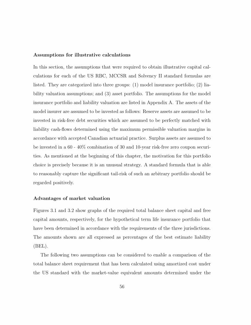
Assumptions for illustrative calculations
In this section, the assumptions that were required to obtain illustrative capital cal-
culations for each of the US RBC, MCCSR and Solvency II standard formulas are
listed. They are categorized into three groups: (1) model insurance portfolio; (2) lia-
bility valuation assumptions; and (3) asset portfolio. The assumptions for the model
insurance portfolio and liability valuation are listed in Appendix A. The assets of the
model insurer are assumed to be invested as follows: Reserve assets are assumed to be
invested in risk-free debt securities which are assumed to be perfectly matched with
liability cash-flows determined using the maximum permissible valuation margins in
accordance with accepted Canadian actuarial practice. Surplus assets are assumed to
be invested in a 60 - 40% combination of 30 and 10-year risk-free zero coupon securi-
ties. As mentioned at the beginning of this chapter, the motivation for this portfolio
choice is precisely because it is an unusual strategy. A standard formula that is able
to reasonably capture the significant tail-risk of such an arbitrary portfolio should be
regarded positively.
Advantages of market valuation
Figures 3.1 and 3.2 show graphs of the required total balance sheet capital and free
capital amounts, respectively, for the hypothetical term life insurance portfolio that
have been determined in accordance with the requirements of the three jurisdictions.
The amounts shown are all expressed as percentages of the best estimate liability
(BEL).
The following two assumptions can be considered to enable a comparison of the
total balance sheet requirement that has been calculated using amortized cost under
the US standard with the market-value equivalent amounts determined under the
56
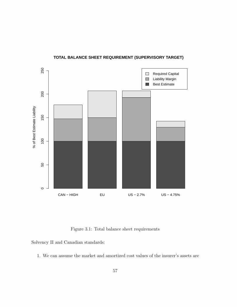
CAN − HIGH EU US − 2.7% US − 4.75%
Required Capital
Liability Margin
Best Estimate
TOTAL BALANCE SHEET REQUIREMENT (SUPERVISORY TARGET)
% o
f Bes
t Est
imat
e Li
abili
ty
050
100
150
200
250
Figure 3.1: Total balance sheet requirements
Solvency II and Canadian standards:
1. We can assume the market and amortized cost values of the insurer’s assets are
57
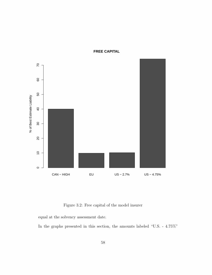
CAN − HIGH EU US − 2.7% US − 4.75%
FREE CAPITAL
% o
f Bes
t Est
imat
e Li
abili
ty
010
2030
4050
6070
Figure 3.2: Free capital of the model insurer
equal at the solvency assessment date.
In the graphs presented in this section, the amounts labeled “U.S. - 4.75%”
58
are directly comparable to the corresponding amounts under Canadian and EU
Solvency II rules, subject to the assumption of equal market and amortized
cost values. This might be the case if, prior to December 31, 2008, the insurer
had been investing in and rolling over one-year Treasury bills upon maturity.
Given that risky investment strategy, the AVR and IMR would have been nil on
December 31, 2008, when the portfolio is rebalanced to the assumed matched
strategy.
2. The valuation rate for calculating formula-based reserves can be adjusted to
reflect current interest rates. The amounts labeled in the graphs as “U.S. -
2.7%” are comparable to the corresponding Canadian and Solvency II amounts
in the sense that they have been calculated using the same reference interest
rates. The 2.7% rate corresponds to the 10-year swap rate in Table A.1 of the
appendix.
The risk management benefits of basing a solvency assessment on market values
are illustrated in Figures 3.1 and 3.2:
1. To demonstrate the risk management benefits of a market valuation balance
sheet, we first need an economic measure of liabilities. Let us assume that the
Solvency II liability is a good proxy for this economic liability i.e. MVL(ic, lc,mc)
≈ SLeu(ic, lc,mc). Figure 3.1 then implies that the financial position of the in-
surer (i.e. net assets) is grossly overstated when the solvency liabilities are
determined using the U.S. formula-based approach (based on ip= 4.75%). In
fact, TBSRus(ip = .0475, lp = 0,mp) ≤ MVL(ic, lc,mc) . The main reason for
the significantly lower capital requirements under the U.S. rules is the relatively
high statutory (lagged) interest rate of 4.75% that was used to determine liabil-
59
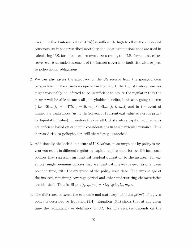
ities. The fixed interest rate of 4.75% is sufficiently high to offset the embedded
conservatism in the prescribed mortality and lapse assumptions that are used in
calculating U.S. formula-based reserves. As a result, the U.S. formula-based re-
serves cause an understatement of the insurer’s overall default risk with respect
to policyholder obligations.
2. We can also assess the adequacy of the US reserve from the going-concern
perspective. In the situation depicted in Figure 3.1, the U.S. statutory reserves
might reasonably be inferred to be insufficient to assure the regulator that the
insurer will be able to meet all policyholder benefits, both as a going-concern
( i.e. SLus(ip = .0475, lp = 0,mp) ≤ SLcan(ic, lc,mc)) and in the event of
immediate bankruptcy (using the Solvency II current exit value as a crude proxy
for liquidation value). Therefore the overall U.S. statutory capital requirements
are deficient based on economic considerations in this particular instance. This
increased risk to policyholders will therefore go unnoticed.
3. Additionally, the locked-in nature of U.S. valuation assumptions by policy issue-
year can result in different regulatory capital requirements for two life insurance
policies that represent an identical residual obligation to the insurer. For ex-
ample, single premium policies that are identical in every respect as of a given
point in time, with the exception of the policy issue date. The current age of
the insured, remaining coverage period and other underwriting characteristics
are identical. That is, SL[x]+t(ip, lp,mp) = SL[x+t](ip′ , lp′ ,mp′).
4. The difference between the economic and statutory liabilities ρ(im′) of a given
policy is described by Equation (3.4). Equation (3.4) shows that at any given
time the redundancy or deficiency of U.S. formula reserves depends on the
60

relationship between the prescribed and current valuation assumptions.
ρ(im′) = MVL(ic, lc,mc)− SLus(ip, lp,mp) (3.4)
For example, when interest rates are falling (i.e. ip − ic ≥ 0) there will be
a bias towards undervaluing liabilities (i.e ρ(im′) ≥ 0). The opposite effect
would be expected when interest rates are increasing (i.e. ic − ip ≥ 0). For a
given insurer at any given moment, the aggregate deficiency or redundancy of
reserves with respect to interest rates will depend on the history of interest rates
as well as the volume of new business that was issued in each previous year.
If interest rates are assumed to be cyclical, the net redundancy or deficiency
could be expected to cancel out over time for a mature insurer. However, since
interest rates can have prolonged periods in which they are either trending up
or down, the assumption that the deficiencies and redundancies will cancel is
not guaranteed.
5. When the statutory valuation interest rates under the U.S. framework are much
lower than market rates, resulting in conservative reserves, insurers in financial
difficulty may be incentivized to arbitrage the regulatory capital requirements
through reinsurance, securitization or other innovative capital market transac-
tions. An economic valuation of assets and liabilities that uses current assump-
tions may be expected to mitigate the possibility of regulatory arbitrage by
insurers.
6. The MCCSR amounts in Figures 3.1 and 3.2 are based on the most-conservative
valuation assumptions in accordance with generally accepted Canadian actuar-
ial practice ASB (Canada) (2009). The MCCSR amounts would be lower if
61

more aggressive assumptions had been used, resulting in more free capital for
shareholders. Therefore, there appears to be an incentive for shareholders to
understate reserves when policy liabilities are subjective.
Since the determination of the Canadian GAAP liability requires the subjective
input of the actuary, it is possible to have multiple balance sheet measurements
of the same liability. Subjective liabilities also make it difficult to obtain robust
comparisons of financial strength across insurers.
7. Figure 3.2 shows that the amount of the insurer’s free capital for the U.S.- 4.75%
case is significantly greater than the amounts for the other standard formulas.
The real danger of misclassifying capital or liabilities as free capital is that the
money may be permanently withdrawn by shareholders.
3.2.3 Capital requirements
In this section, the appropriateness of the standard formula capital requirements is
determined using the proposed global capital framework as the benchmark.
Calibration horizon and cash-flow versus market valuation perspectives
Solvency II uses a calibration period of one year (CEIOPS (2010)). Equation (A.13)
in the appendix illustrates the calculation of credit spread risk under Solvency II.
The need to determine capital for spread risk under Solvency II is because risk is
defined under that standard in terms of changes in market values over a one-year
period. The calibration of the formula is such that the resulting capital requirement
corresponds to VaR 99.5% of the market-value losses due to spread risk over a one-
year period. In contrast, the calibration of the credit default risk factors under the
62
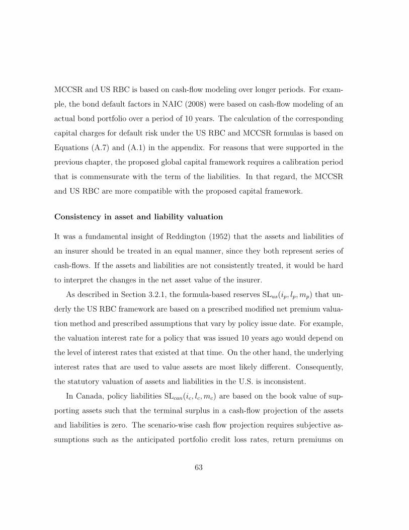
MCCSR and US RBC is based on cash-flow modeling over longer periods. For exam-
ple, the bond default factors in NAIC (2008) were based on cash-flow modeling of an
actual bond portfolio over a period of 10 years. The calculation of the corresponding
capital charges for default risk under the US RBC and MCCSR formulas is based on
Equations (A.7) and (A.1) in the appendix. For reasons that were supported in the
previous chapter, the proposed global capital framework requires a calibration period
that is commensurate with the term of the liabilities. In that regard, the MCCSR
and US RBC are more compatible with the proposed capital framework.
Consistency in asset and liability valuation
It was a fundamental insight of Reddington (1952) that the assets and liabilities of
an insurer should be treated in an equal manner, since they both represent series of
cash-flows. If the assets and liabilities are not consistently treated, it would be hard
to interpret the changes in the net asset value of the insurer.
As described in Section 3.2.1, the formula-based reserves SLus(ip, lp,mp) that un-
derly the US RBC framework are based on a prescribed modified net premium valua-
tion method and prescribed assumptions that vary by policy issue date. For example,
the valuation interest rate for a policy that was issued 10 years ago would depend on
the level of interest rates that existed at that time. On the other hand, the underlying
interest rates that are used to value assets are most likely different. Consequently,
the statutory valuation of assets and liabilities in the U.S. is inconsistent.
In Canada, policy liabilities SLcan(ic, lc,mc) are based on the book value of sup-
porting assets such that the terminal surplus in a cash-flow projection of the assets
and liabilities is zero. The scenario-wise cash flow projection requires subjective as-
sumptions such as the anticipated portfolio credit loss rates, return premiums on
63
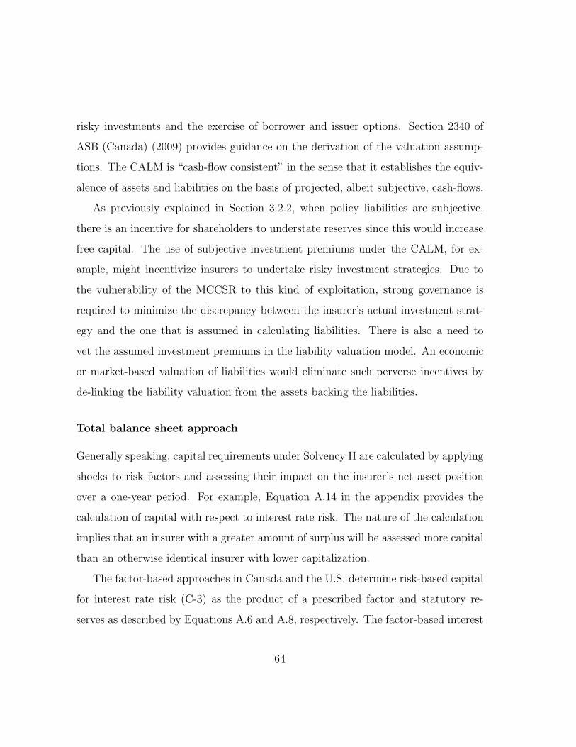
risky investments and the exercise of borrower and issuer options. Section 2340 of
ASB (Canada) (2009) provides guidance on the derivation of the valuation assump-
tions. The CALM is “cash-flow consistent” in the sense that it establishes the equiv-
alence of assets and liabilities on the basis of projected, albeit subjective, cash-flows.
As previously explained in Section 3.2.2, when policy liabilities are subjective,
there is an incentive for shareholders to understate reserves since this would increase
free capital. The use of subjective investment premiums under the CALM, for ex-
ample, might incentivize insurers to undertake risky investment strategies. Due to
the vulnerability of the MCCSR to this kind of exploitation, strong governance is
required to minimize the discrepancy between the insurer’s actual investment strat-
egy and the one that is assumed in calculating liabilities. There is also a need to
vet the assumed investment premiums in the liability valuation model. An economic
or market-based valuation of liabilities would eliminate such perverse incentives by
de-linking the liability valuation from the assets backing the liabilities.
Total balance sheet approach
Generally speaking, capital requirements under Solvency II are calculated by applying
shocks to risk factors and assessing their impact on the insurer’s net asset position
over a one-year period. For example, Equation A.14 in the appendix provides the
calculation of capital with respect to interest rate risk. The nature of the calculation
implies that an insurer with a greater amount of surplus will be assessed more capital
than an otherwise identical insurer with lower capitalization.
The factor-based approaches in Canada and the U.S. determine risk-based capital
for interest rate risk (C-3) as the product of a prescribed factor and statutory re-
serves as described by Equations A.6 and A.8, respectively. The factor-based interest
64
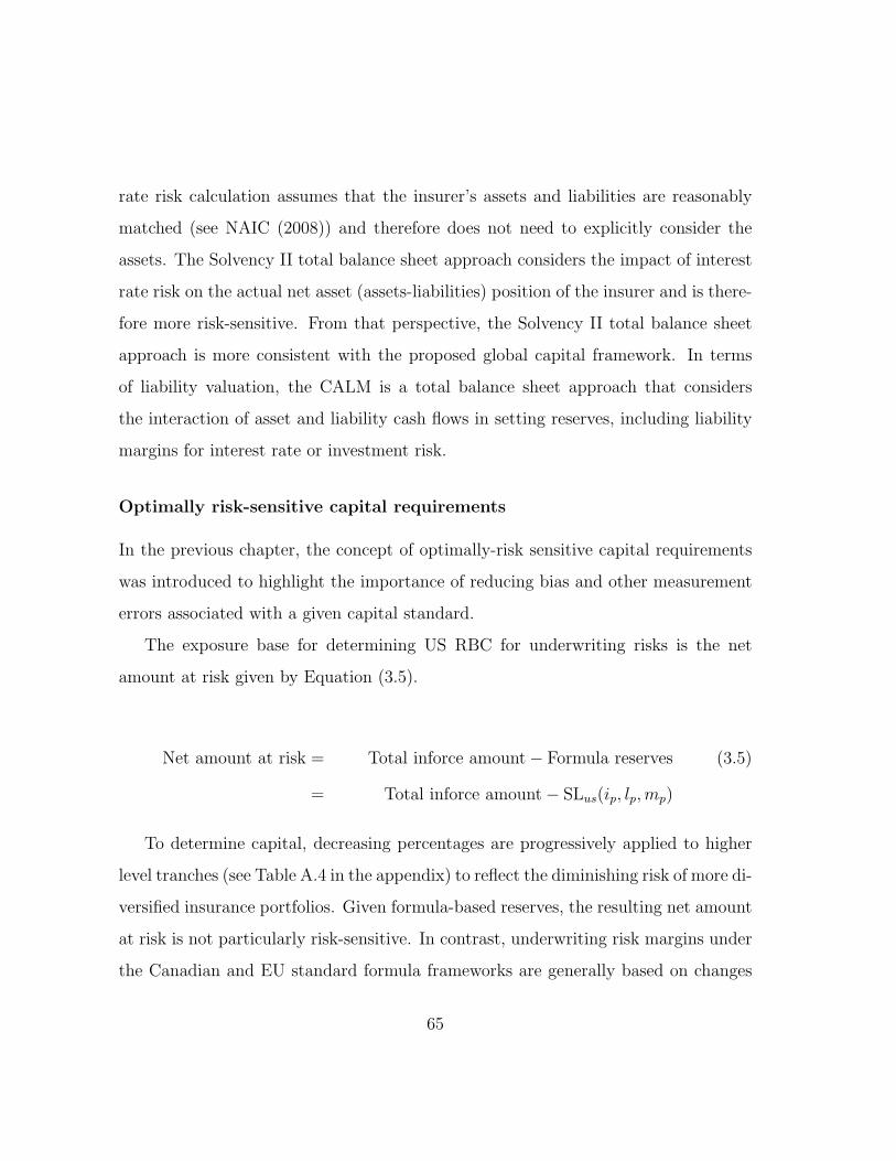
rate risk calculation assumes that the insurer’s assets and liabilities are reasonably
matched (see NAIC (2008)) and therefore does not need to explicitly consider the
assets. The Solvency II total balance sheet approach considers the impact of interest
rate risk on the actual net asset (assets-liabilities) position of the insurer and is there-
fore more risk-sensitive. From that perspective, the Solvency II total balance sheet
approach is more consistent with the proposed global capital framework. In terms
of liability valuation, the CALM is a total balance sheet approach that considers
the interaction of asset and liability cash flows in setting reserves, including liability
margins for interest rate or investment risk.
Optimally risk-sensitive capital requirements
In the previous chapter, the concept of optimally-risk sensitive capital requirements
was introduced to highlight the importance of reducing bias and other measurement
errors associated with a given capital standard.
The exposure base for determining US RBC for underwriting risks is the net
amount at risk given by Equation (3.5).
Net amount at risk = Total inforce amount− Formula reserves (3.5)
= Total inforce amount− SLus(ip, lp,mp)
To determine capital, decreasing percentages are progressively applied to higher
level tranches (see Table A.4 in the appendix) to reflect the diminishing risk of more di-
versified insurance portfolios. Given formula-based reserves, the resulting net amount
at risk is not particularly risk-sensitive. In contrast, underwriting risk margins under
the Canadian and EU standard formula frameworks are generally based on changes
65
in the reserve requirements due to a prescribed change in the underlying risk fac-
tors, and are therefore more risk sensitive and portfolio-specific. For example, the
calculation of mortality parameter risk under the Solvency II formula is provided by
Equation (A.10). In the fifth quantitative impact study of Solvency II (i.e. QIS 5),
the mortality shock which should be applied to the balance sheet has been changed
from 10% to 15%. In Canada, mortality parameter risk is included in the CALM
liability, with the remaining two components of mortality risk (i.e. volatility and
catastrophic risks) being included in capital requirements (OSFI (2010b)).
Categories of risk
A capital framework should include all material risk exposures. Equation (1.1) shows
that the US RBC for life insurance formula does not include catastrophe and oper-
ational risks. However, the U.S. RBC formula includes a charge for general business
risk (C4) which is not included in the Solvency II or MCCSR formulas. In Canada, an
arbitrary loading of 50% is applied to capital requirements that have been determined
in accordance with Equation (1.3) to account for qualitative risk exposures.
The Solvency II standard formula does not include a margin for mortality volatility
or process risk which is explicitly included in the MCCSR formula. The significance
of this component can be expected to rise with increased skewness in the distribution
of life insurance amounts and with decreasing size of the portfolio.
Diversification credits
The calibration of the dependencies among risks is primarily a qualitative exercise.
The difficulty in measuring tail dependencies was discussed in Chapter 1. From the
point of view of incentives, Equation (2.9), implies that there will be no incentive
66
to diversify if perfect correlation is assumed among risk types. On the other hand,
significant diversification incentives will encourage insurers to bulk up, and perhaps
squeeze out smaller players out of the market. The appropriate amount of incentives
to provide for diversification will be determined by the specifics of the insurance
market, among other considerations.
Equation (1.10) suggests the potential for significant diversification credits under
Solvency II. The assumed correlation structure of risks under Solvency II describes
the joint behaviour of the risks under a financially adverse scenario of events. Specif-
ically, the tail correlations are calibrated such that they produce a solvency capital
requirement at the enterprise level that has an associated ruin probability of 0.5%
over a one year period. In general, the diversification incentives that are provided
under the U.S. RBC formula (described by Equation (1.1)) are more modest than
the amounts under Solvency II. Equation (1.3) shows that there are no diversification
credits under Canada’s MCCSR formula since the total capital requirement is simply
the sum of its component requirements.
Enterprise-level ruin probability
The solvency capital requirement under Solvency II is calculated to achieve a 99.5%
confidence level over a one-year period at the enterprise level. In contrast, the total
solvency buffer (i.e. TBSRi - BEL, for i=CAN, US ) under the Canadian and US
regimes has no explicit confidence level attached to it. If there is no specific targeted
security level, then it is plausible to expect that such systems will result in significant
levels of redundancies and/or deficiencies that cause capital to be misallocated.
67

3.3 Chapter conclusion
For reasons described in Chapter 2, and based on the analysis of this chapter, an eco-
nomic or market-based valuation framework that meets the conditions stipulated in
the global framework attributes (GFAs) appears to be a reasonable unifying basis for
a global capital framework. A long-term, cash-flow based economic valuation frame-
work is preferable from a risk management perspective since it provides a relatively
more objective, transparent and consistent solvency benchmark for determining ap-
propriate capital requirements. A single global capital framework would also tend to
mitigate the extent of arbitrage that is possible by international insurers.
68
Chapter 4
Proposal of an asset-liability
mismatch risk measurement
framework
4.1 Overview
4.1.1 Motivation
The global capital framework that was proposed in Chapter 2 will be applied to
the specific measurement of asset-liability mismatch (ALM) risk in this chapter.
The proposed ALM risk measurement approaches under the U.S. Principle-Based
Approach (US PBA) (AAA (2008a)), Future Internal Model Approach (FIMA) in
Canada (JCOAA (2008a,b); MAC (2007)) and Solvency II (e.g. CEIOPS (2010)),
will be critically compared against the incentive-based capital framework that was
proposed in Chapter 2. The main features of the (internal-model) regulatory capital
69
standards that have been proposed in the U.S., Canada and the EU are summarized
in Table 4.2. The proposed capital standard in Canada is preliminary and has not
been finalized.
As the complexity of the features that are embedded in insurance contracts has
increased, so has the sophistication of the risk management programs that are used to
hedge those features. As part of the asset-liability management programs of insurers
worldwide, the embedded derivatives in insurance contracts are frequently hedged
using portfolios of interest rate and credit default swaps, options, futures and other
capital market instruments. To promote innovation and prudent risk management
by the insurer, the regulatory capital framework must properly reflect the risk miti-
gating impact of these strategies on the insurer’s overall risk profile. In the context
of Equation 2.12, all three measurement errors (∆εCF , ∆εA and ∆εL) can be ex-
pected to be large when a significant proportion of the insurer’s portfolio consists of
over-the-counter (OTC) and other derivatives that are suitable for matching complex
insurance liabilities. A comparison of alternative capital standards should therefore
consider the potential exposure to measurement error of each standard. Additionally,
the incentive effect of the ALM risk capital requirements should be considered for the
same reasons that were outlined in previous chapters. For example, it was argued in
Chapter 2 under GFA 3 that a solvency capital framework should be compatible with
the generally long-term cash-flow nature of insurance business. In this regard, a cap-
ital standard that is calibrated to short-term market movements can inappropriately
incentivise insurers to take a myopic view of their risk exposures.
The primary goals of this chapter are twofold:
1. To apply the global capital framework that was proposed in Chapter 2 to the
specific measurement of the ALM risk of life insurers. The proposed ALM risk
70
capital standards in the U.S., Canada and the EU will also be reviewed against
this proposed benchmark standard to highlight their deficiencies.
2. The appropriateness of the incentive structures that are implied by the pro-
posed ALM risk capital requirements in the U.S., Canada and the EU will also
be examined using the framework for policyholder-oriented incentives that was
outlined in Chapter 2. Doff (2008) reviewed the extent to which Solvency II
satisfied the seven objectives of risk-based capital proposed by Cummins et al.
(1993). He concluded that Solvency II generally satisfies the criteria. A different
conclusion is reached in this chapter regarding the appropriateness of the in-
centives of the Solvency II framework (i.e. the first objective in Cummins et al.
(1993)) with respect to the measurement of ALM risk.
4.1.2 Outline of chapter
The remainder of this chapter is structured as follows. The assumptions of the model
insurer for which the monte-carlo simulation experiments that underly the results of
this chapter were performed are provided in Section 4.2. The definitions of supervisory
target capital that are used in this chapter are provided in Section 4.3. In Section 4.4,
alternative ALM risk capital standards including the proposed US PBA, Canadian
and Solvency II standards, will be critically reviewed against the benchmark standard
that was proposed in Chapter 2. The term structure of insolvency risk decomposition
of the proposed ALM risk measurement framework will be used to reconcile observed
differences among the alternative capital standards. In Section 4.5, the potential
impact of model error on relative ALM risk and capital assessments will be discussed.
The main conclusions of this chapter are outlined in Section 4.6.
71

4.2 Model insurer
4.2.1 Model insurance portfolio
The monte-carlo analysis conducted in this chapter is based on a model life insurance
company that issues only 20-year term life insurance. The 20-year term product is
being used as a proxy for long-dated insurance products. It is assumed that the model
insurer has been in business for the last 20 years and has been growing at a rate of
5% per year (number of policies) during that period. The number of policies issued
in the most recent period is assumed to be 10,000. Therefore, the number of policies
issued in a given previous year is 10,000 × 1.05−t, where t is the number of years
preceding the most recent period.
• The original term of the insurance policies is 20 years
• The premiums are level and the product is not renewable
• The face amount of each policy is $500,000
• The annual premium is $1.80 per $1,000 face amount
• Expenses are 5% of the gross premium for all renewal years
• Issue age: 35
• All death benefits are assumed to be paid at the end of the year of death, while
premiums and expenses are paid at the beginning of the year
The cashflows of the term life insurance portfolio are projected assuming a lapse
rate of 4% per year, and mortality in accordance with Table B.1 in the appendix.
72

The monte-carlo simulation also assumes that there will be no further issuance of
new policies in future periods so that the insurance portfolio will be managed on a
run-off basis.
4.2.2 Assumed investment strategies of the model insurer
In this chapter, reference will be made to six alternative investment strategies (Θi
for i=1,..,6) of the model insurance company: the “bullet”, “barbell”, “laddered”,
“short bond”, “long bond” and “duration matching” portfolio strategies. The first
five of these strategies are more or less static (i.e. buy and hold) in the sense that no
portfolio rebalancing is assumed to occur other than the reinvestment or divestment
of net cash flows (investment income plus par redemptions less insurance cashflows)
to the insurer. Reinvestment cash flows are used to purchase (hypothetical) bonds
of a maturity which corresponds to the residual maturity of the portfolio holdings at
the time, while existing bond holdings are sold as needed to fund net cash outflows
to the policyholders.
The details of the portfolio strategies are as follows:
1. Bullet strategy (Θ1): The initial portfolio of this strategy consists entirely of
hypothetical 14-year risk-free (annual) coupon bonds. After 14 years when the
bond matures, the proceeds are reinvested in 5 year bonds. As needed, bonds
are sold to fund insurance policyholder benefits.
2. Barbell strategy (Θ2): The initial portfolio consists of 1-year (23.9%) and
20-year (76.1%) risk-free coupon bonds.
3. Laddered strategy (Θ3): The initial portfolio is invested in risk-free coupon
bonds of the following maturities, with the proportion corresponding to each
73
maturity indicated in parentheses: 1-year (5%), 3-year (5%), 5-year (10%), 7-
year (15%), 10-year (10%), 15-year (10%), 20-year (20%) and 30-year (25%).
4. Short bond strategy (Θ4): Under this strategy, the entire portfolio is invested
in 5-year risk-free (annual) coupon bonds. At every five-year anniversary there-
after, when the remaining bonds have matured, the portfolio is rolled over into
new five year bonds.
5. Long bond strategy (Θ5): The initial portfolio consists entirely of 30-year
risk-free (annual) coupon bonds.
6. Duration matching strategy (Θ6): Under the duration matching strategy,
the portfolio is rebalanced annually to match the duration of the liabilities. At
any given time, the minimum bond maturity that has a duration that is greater
or equal to that of the liabilities under the prevailing interest rate environment
is determined. If the duration of the determined bond maturity is greater than
the liability duration, an exact duration match is achieved by a proportionate
investment in one-year bonds, with the remainder of the portfolio being allo-
cated to the determined bond maturity. The initial portfolio under this strategy
consists of 1-year (2.7%) and 14-year (97.3%) default-free bonds.
In the monte-carlo simulation study, all bonds are assumed to be purchased at par
or face value. The interest rates that were used as the starting point for the simulation
are shown in the appendix in Table B.2. The coupon rates for the bonds purchased
on the start date of the simulation correspond to the par yield column in Table B.2.
Beyond the start date, the C-3 Phase III interest rate generator was used to obtain
10,000 stochastic scenarios. The C-3 Phase III generator has been recommended by
the Life Reserve Working Group (LRWG) of the American Academy of Actuaries
74
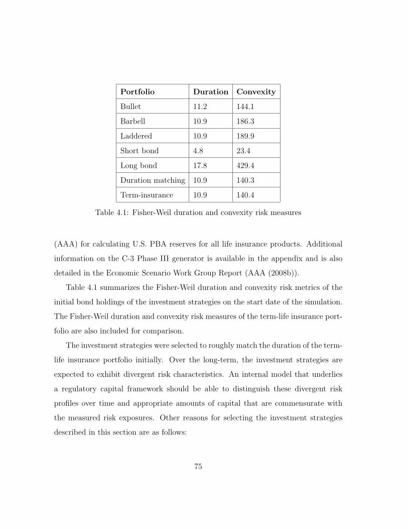
Portfolio Duration Convexity
Bullet 11.2 144.1
Barbell 10.9 186.3
Laddered 10.9 189.9
Short bond 4.8 23.4
Long bond 17.8 429.4
Duration matching 10.9 140.3
Term-insurance 10.9 140.4
Table 4.1: Fisher-Weil duration and convexity risk measures
(AAA) for calculating U.S. PBA reserves for all life insurance products. Additional
information on the C-3 Phase III generator is available in the appendix and is also
detailed in the Economic Scenario Work Group Report (AAA (2008b)).
Table 4.1 summarizes the Fisher-Weil duration and convexity risk metrics of the
initial bond holdings of the investment strategies on the start date of the simulation.
The Fisher-Weil duration and convexity risk measures of the term-life insurance port-
folio are also included for comparison.
The investment strategies were selected to roughly match the duration of the term-
life insurance portfolio initially. Over the long-term, the investment strategies are
expected to exhibit divergent risk characteristics. An internal model that underlies
a regulatory capital framework should be able to distinguish these divergent risk
profiles over time and appropriate amounts of capital that are commensurate with
the measured risk exposures. Other reasons for selecting the investment strategies
described in this section are as follows:
75
1. The short and long bond strategies can be considered to be proxies for high
risk investment or risk management strategies of an insurer. From a supervi-
sory standpoint, it is especially important for an internal model to be able to
accurately capture the increased insolvency tail-risk of these strategies through
commensurately increased capital requirements. Given typically long-term in-
surance liabilities, the short bond strategy can also be viewed as a representative
depiction of the very real-life situation that exists in many insurance markets
where there are no investable assets of sufficient duration to match that of the
liabilities. In those insurance markets where this is the case, the reinvestment
risk is intrinsic to the insurance market. On the other hand, the long bond
strategy creates an asset-liability mismatch exposure to price risk, akin to the
situation that is faced by banking institutions that borrow short and lend long
when the yield curve is upward sloping.
2. The duration matching strategy is a risk management strategy that has been se-
lected to assess the relative impact of hedging ALM risk on capital requirements
under the different internal model-based capital frameworks.
4.3 Definitions of supervisory target capital
In this section, the measurement of ALM risk under the proposed Canadian, U.S.
and Solvency II regulatory capital frameworks will be reviewed. A summary of the
important features of these proposed capital frameworks is provided in Table 4.2.
The total capital requirements under each proposed capital standard will be com-
pared using the Total Balance Sheet Requirement (TBSR). The Scenario Total Bal-
ance Sheet Requirement quantity (i.e. ALM risk loss random variable) will be first
76

U.S. Canada EU
Liability valuation Actuarial Valuation
Approach (AVA)
(AVA is the statutory
value of assets needed
to pay benefits at a
CTE X% confidence
level)
IFRS GAAP Liability
(BEL + IFRS MVM)
(details to be finalised
with issuance of IFRS
Insurance Contracts
Phase II)
Market Value Liabil-
ity (BEL+SII MVM)
(i.e. Solvency II trans-
fer value)
Asset valuation Statutory (combina-
tion of book, equity,
historical cost, fair
value)
IFRS Fair Value Market Value
Solvency assessment
basis
Total asset require-
ment
Total asset require-
ment = best estimate
liability (BEL) + cap-
ital buffer (but capital
ratios will continue to
used)
Total asset require-
ment= BEL + MVM
+ SCR
Risk metric CTE CTE VAR
Solvency assessment
horizon
Lifetime of liability 1 year 1 year
Confidence level 90% 99% 99.5%
Investments Quantitative limits
and restrictions
To be determined No restrictions
Internal models only C3-risk for
now, and by product
(model segment); var-
ious floors for capital
and reserves
By risk, and not ex-
pected to be imple-
mented before 2014;
floor based on stan-
dard formula
Enterprise-wide model
(option to use partial
internal model); only
floor is the MCR
Risk mitigation Can be reflected in the
cash flow model over
the liability term
Only instruments held
on valuation date can
be recognised
Can be reflected over
the 1-year horizon
Table 4.2: A summary of the proposed capital requirements
77
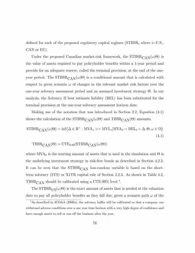
defined for each of the proposed regulatory capital regimes (STBSRi where i=U.S.,
CAN or EU).
Under the proposed Canadian market-risk framework, the STBSRCAN(ω|Θ) is
the value of assets required to pay policyholder benefits within a 1-year period and
provide for an adequate reserve, called the terminal provision, at the end of the one-
year period. The STBSRCAN(ω|Θ) is a conditional amount that is calculated with
respect to given scenario ω of changes in the relevant market risk factors over the
one-year solvency assessment period and an assumed investment strategy Θ. In our
analysis, the Solvency II best estimate liability (BEL) has been substituted for the
terminal provision at the one-year solvency assessment horizon date.
Making use of the notation that was introduced in Section 2.2, Equation (4.1)
shows the calculation of the STBSRCAN(ω|Θ) and TBSRCAN(Θ) amounts.
STBSRCAN(ω|Θ) = inf∆ ∈ R+ : MVA1 >= MVL1|MVA0 = BEL0 +∆,Θ, ω ∈ Ω
(4.1)
TBSRCAN(Θ) = CTE0.99(STBSRCAN(ω|Θ))
where MVA0 is the starting amount of assets that is used in the simulation and Θ is
the underlying investment strategy in risk-free bonds as described in Section 4.2.2.
It can be seen that the STBSRCAN loss-random variable is based on the short-
term solvency (STS) or X1YR capital rule of Section 2.2.3. As shown in Table 4.2,
TBSRCAN should be calibrated using a CTE-99% level 1.
The STBSRUS(ω|Θ) is the exact amount of assets that is needed at the valuation
date to pay all policyholder benefits as they fall due, given a scenario path ω of the
1As described in JCOAA (2008a), the solvency buffer will be calibrated so that a company can
withstand adverse conditions over a one year time horizon with a very high degree of confidence and
have enough assets to sell or run off the business after the year.
78
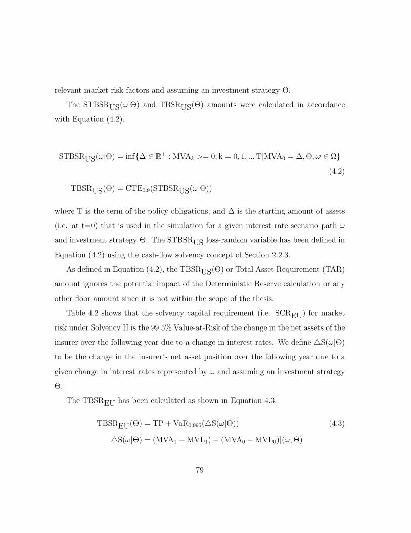
relevant market risk factors and assuming an investment strategy Θ.
The STBSRUS(ω|Θ) and TBSRUS(Θ) amounts were calculated in accordance
with Equation (4.2).
STBSRUS(ω|Θ) = inf∆ ∈ R+ : MVAk >= 0; k = 0, 1, ..,T|MVA0 = ∆,Θ, ω ∈ Ω
(4.2)
TBSRUS(Θ) = CTE0.9(STBSRUS(ω|Θ))
where T is the term of the policy obligations, and ∆ is the starting amount of assets
(i.e. at t=0) that is used in the simulation for a given interest rate scenario path ω
and investment strategy Θ. The STBSRUS loss-random variable has been defined in
Equation (4.2) using the cash-flow solvency concept of Section 2.2.3.
As defined in Equation (4.2), the TBSRUS(Θ) or Total Asset Requirement (TAR)
amount ignores the potential impact of the Deterministic Reserve calculation or any
other floor amount since it is not within the scope of the thesis.
Table 4.2 shows that the solvency capital requirement (i.e. SCREU) for market
risk under Solvency II is the 99.5% Value-at-Risk of the change in the net assets of the
insurer over the following year due to a change in interest rates. We define S(ω|Θ)
to be the change in the insurer’s net asset position over the following year due to a
given change in interest rates represented by ω and assuming an investment strategy
Θ.
The TBSREU has been calculated as shown in Equation 4.3.
TBSREU(Θ) = TP + VaR0.995(S(ω|Θ)) (4.3)
S(ω|Θ) = (MVA1 −MVL1)− (MVA0 −MVL0)|(ω,Θ)
79
where TP corresponds to the Solvency II technical provisions that were defined in
Section 3.2.1. The Solvency II best-estimate liability (BEL) has been substituted for
the TP amount since the focus of this chapter is on the measurement of ALM risk.
4.4 A numerical comparison of the proposed ALM
risk capital requirements
In this section, we will take a closer look at some of the more fundamental aspects
of the proposed regulatory capital standards for ALM risk. The analysis presented
is based on monte-carlo simulation results of the model insurance company that was
described in Section 4.2. The model insurer will be assumed to invest its assets in
accordance with the long-bond strategy in cases where it is not necessary to reflect
the impact of varying the investment strategy. In a risk-based solvency supervision
framework, the long-bond strategy should command the greatest attention of the
regulator since it is the most unmatched strategy.
4.4.1 Sample distribution of supervisory target capital
Figure 4.1 shows the distribution of the scenario-specific total balance sheet require-
ment (STBSR) for each of the three proposed capital adequacy regimes.
The model insurer is assumed to commit its entire asset portfolio to the long-bond
investment strategy that has been described in Section 4.2.
The assumed initial market-consistent values of the insurer’s assets and liabilities
are shown in Table 4.3.
The distributions of STBSREU and STBSRCAN have been left-truncated at the
80
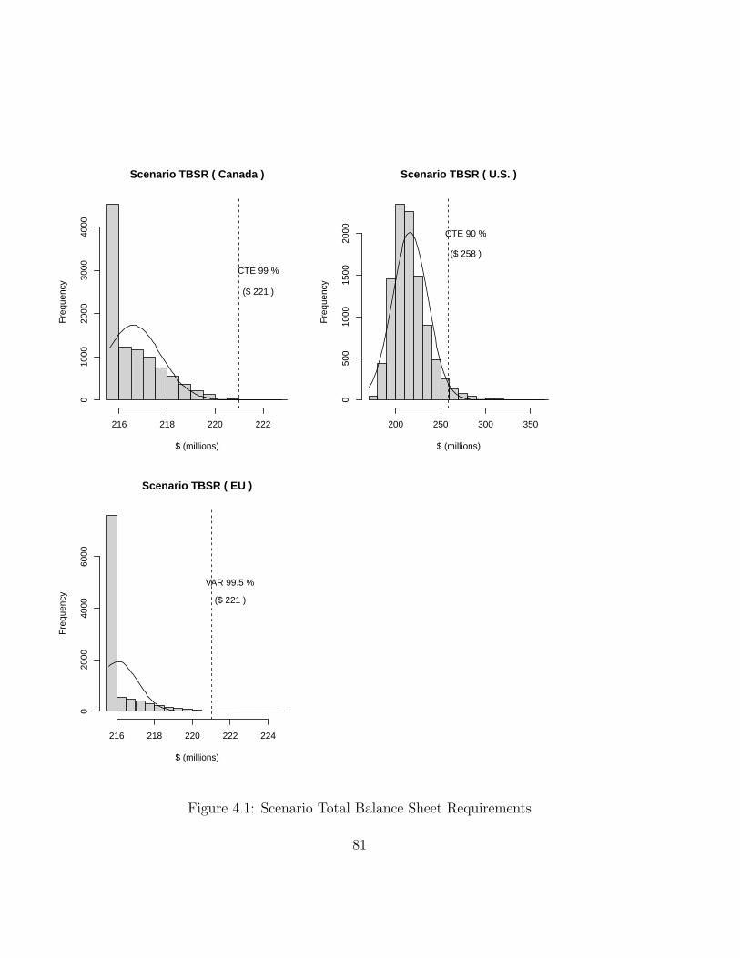
Scenario TBSR ( Canada )
$ (millions)
Fre
quen
cy
216 218 220 222
010
0020
0030
0040
00
CTE 99 %
($ 221 )
Scenario TBSR ( U.S. )
$ (millions)
Fre
quen
cy
200 250 300 350
050
010
0015
0020
00 CTE 90 %
($ 258 )
Scenario TBSR ( EU )
$ (millions)
Fre
quen
cy
216 218 220 222 224
020
0040
0060
00
VAR 99.5 %
($ 221 )
Figure 4.1: Scenario Total Balance Sheet Requirements
81

Market value of assets 266,004,000
Best estimate of liabilities 215,599,000
Net Assets 50,405,000
Table 4.3: Initial balance sheet of the model insurer
amount of the market-consistent technical provisions thus generating a probability
mass-point at $215,599,000. Under the proposed Canadian and Solvency II frame-
works, it seems reasonable that a solvent insurer should have an amount of assets that
is at least sufficient to sell or runoff the business on the solvency assessment date.
In the case of the long-bond strategy, Figure 4.1 shows that the U.S. PBA total
capital amount of $258 million is the highest of the three regimes. The Canadian and
Solvency II total capital amounts are each $221 million when rounded to the nearest
1 million dollars. In other words, for the same ALM risk exposure, the U.S. PBA
requires an additional $37 million of capital, which is 17.0% of the liabilities. This
example clearly highlights the extent of regulatory capital arbitrage that is possible
given the different perspectives of risk under the three regimes.
Equations 4.1 and 4.3 show that there are two main sources of difference between
the Canadian and Solvency II capital requirements:
1. The proposed Canadian framework utilizes the Conditional Tail Expectation as
the risk measure while the Value-at-Risk metric is the basis of the target capital
requirement under Solvency II.
2. The Solvency II capital requirement includes an incremental capital charge on
free assets i.e. those assets over and above the target requirement. Equation 4.1
shows that the proposed Canadian standard does not include this incremental
82

capital charge.
In the example given, the two differences between the Canadian and Solvency
II capital calculations offset each other producing roughly identical target capital
amounts.
The superimposed normal distributions in Figure 4.1 suggest that the insurer’s
ALM risk exposure is skewed when determined under each of the three capital ade-
quacy regimes given the long-bond investment strategy.
4.4.2 Insolvency risk profiles implied by supervisory target
capital amounts of proposed standards
The supervisory target capital amounts or TBSRs that were determined in the previ-
ous section will be used to “bootstrap” an implied solvency risk profile of the model
insurer that corresponds to the TBSR of each capital regime. Figure 4.2 shows the
time variation of the asset-to- economic liability (AL) ratios of the model insurance
company for different amounts of starting assets.
The four cases correspond to different assumed amounts of starting assets of
the model insurer: (1) best estimate liability (BEL) of the insurer’s obligations (2)
TBSRCAN (3) TBSRUS; and (4) TBSREU . The one-year solvency assessment period
that underlies the calibration of the target capital requirements under the Canadian
and Solvency II regimes results in an implied long-term solvency profile of the model
insurer that is very concerning as shown in Figure 4.2. The capital requirements
under the proposed Canadian and Solvency II capital regimes can leave the insurer
exposed to significant insolvency risk in future periods. The long-term calibration
perspective of the U.S. PBA capital requirements is evident in Figure 4.2. At any
83
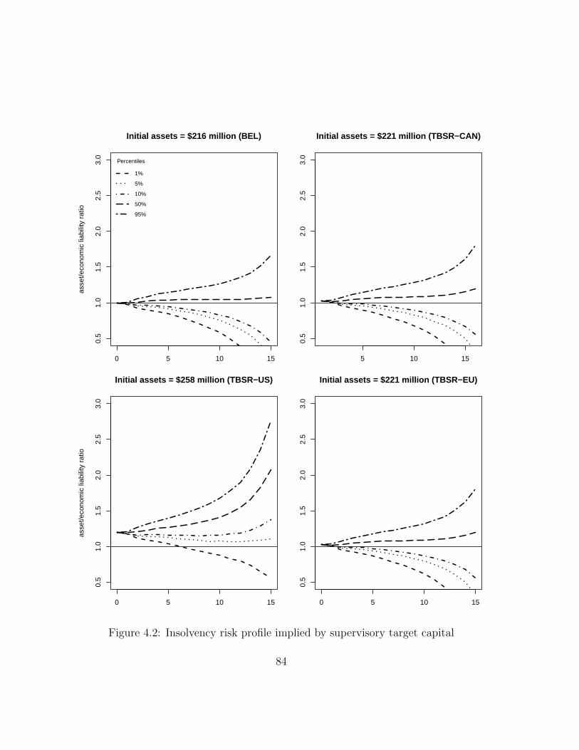
Initial assets = $216 million (BEL)
asse
t/eco
nom
ic li
abili
ty r
atio
0 5 10 15
0.5
1.0
1.5
2.0
2.5
3.0
Percentiles
1%
5%
10%
50%
95%
Initial assets = $221 million (TBSR−CAN)
5 10 15
0.5
1.0
1.5
2.0
2.5
3.0
Initial assets = $258 million (TBSR−US)
asse
t/eco
nom
ic li
abili
ty r
atio
0 5 10 15
0.5
1.0
1.5
2.0
2.5
3.0
Initial assets = $221 million (TBSR−EU)
0 5 10 15
0.5
1.0
1.5
2.0
2.5
3.0
Figure 4.2: Insolvency risk profile implied by supervisory target capital
84
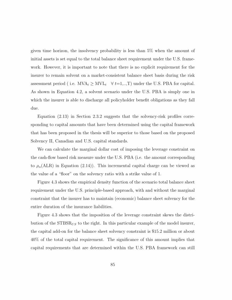
given time horizon, the insolvency probability is less than 5% when the amount of
initial assets is set equal to the total balance sheet requirement under the U.S. frame-
work. However, it is important to note that there is no explicit requirement for the
insurer to remain solvent on a market-consistent balance sheet basis during the risk
assessment period ( i.e. MVAt ≥ MVLt ∀ t=1,..,T) under the U.S. PBA for capital.
As shown in Equation 4.2, a solvent scenario under the U.S. PBA is simply one in
which the insurer is able to discharge all policyholder benefit obligations as they fall
due.
Equation (2.13) in Section 2.3.2 suggests that the solvency-risk profiles corre-
sponding to capital amounts that have been determined using the capital framework
that has been proposed in the thesis will be superior to those based on the proposed
Solvency II, Canadian and U.S. capital standards.
We can calculate the marginal dollar cost of imposing the leverage constraint on
the cash-flow based risk measure under the U.S. PBA (i.e. the amount corresponding
to ρα(ALR) in Equation (2.14)). This incremental capital charge can be viewed as
the value of a “floor” on the solvency ratio with a strike value of 1.
Figure 4.3 shows the empirical density function of the scenario total balance sheet
requirement under the U.S. principle-based approach, with and without the marginal
constraint that the insurer has to maintain (economic) balance sheet solvency for the
entire duration of the insurance liabilities.
Figure 4.3 shows that the imposition of the leverage constraint skews the distri-
bution of the STBSRUS to the right. In this particular example of the model insurer,
the capital add-on for the balance sheet solvency constraint is $15.2 million or about
40% of the total capital requirement. The significance of this amount implies that
capital requirements that are determined within the U.S. PBA framework can still
85
250 300 350 400
0.00
0.01
0.02
0.03
0.04
0.05
0.06
$ (millions)
Den
sity
STBSR − U.S. PBA (including marginal leverage constraint)STBSR − U.S. PBA
Figure 4.3: Incremental capital charge for balance sheet solvency
86
leave the insurer greatly exposed to balance sheet insolvency risk over the term of the
liabilities.
4.4.3 What risk is being measured?
The importance of having a minimum capital requirement that reflects the long-term
cash flow nature of life insurance was underscored by GFA 3 of the global capital
framework that was proposed in Chapter 2. In particular, GFA 3.2 requires the
regulatory capital framework to be based on a risk measure that directly considers
the policyholder cash flows as the primary objective to be met by the insurer.
To assess the extent to which the proposed standards reflect regulatory or pol-
icyholder oriented risk measurements, Figures 4.4 and 4.5 show plots of the model
insurer’s asset to liability ratios (ALRt in Section 2.2) that correspond to the ten
worst-case interest rate scenarios under the proposed U.S. and Solvency II capital
standards respectively.
The interest rate scenarios corresponding to the ten largest STBSRs under each
framework are considered to be the “worst”. As before, the model insurer is assumed
to follow the risky long-bond investment strategy (which should therefore be of more
interest to the prudential regulator). In addition to the adverse interest rate sce-
nario paths, Figure 4.4 also shows the term-liability cash flow profile. The following
important observations can be made from these graphs:
• The interest rate scenarios identified as adverse under each framework are very
different. The worst case scenarios under the U.S. cash flow perspective are
those where interest rates generally increase sharply over the term of the liability
cash flows. The sharp increase in interest rates leads to severely depressed asset
market prices at the times when assets need to be sold to fund net term liability
87
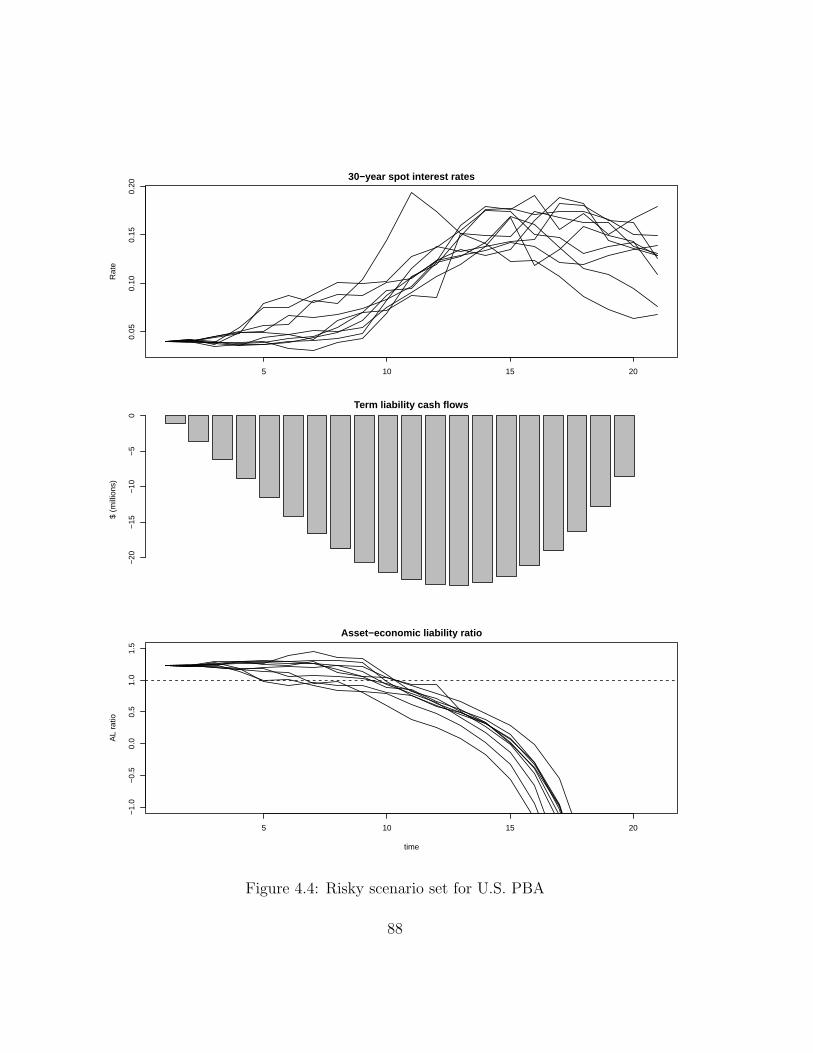
5 10 15 20
0.05
0.10
0.15
0.20
Rat
e
30−year spot interest rates
$ (m
illio
ns)
−20
−15
−10
−5
0
Term liability cash flows
5 10 15 20
−1.
0−
0.5
0.0
0.5
1.0
1.5
Asset−economic liability ratio
time
AL
ratio
Figure 4.4: Risky scenario set for U.S. PBA
88
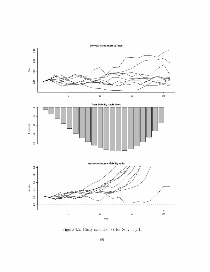
5 10 15 20
0.04
0.06
0.08
0.10
Rat
e
30−year spot interest rates
$ (m
illio
ns)
−20
−15
−10
−5
0
Term liability cash flows
5 10 15 20
1.0
1.2
1.4
1.6
1.8
2.0
Asset−economic liability ratio
time
AL
ratio
Figure 4.5: Risky scenario set for Solvency II
89

cash flows. Under the one-year market valuation risk perspective, an adverse
scenario path is one characterised by a sharp rise in interest rates over a one-year
horizon. As the model insurer is long-duration and convexity risks (based on the
long-bond strategy), the sharp rise in interest rates over the one-year horizon
leads to a significant loss of economic value on a total balance sheet basis. The
one-year measurement horizon for ALM risk that underlies Solvency II and the
proposed Canada framework implies that the progression of interest rates and
the investment strategy beyond the one-year horizon will not be accounted for
under those regimes. The apparent lack of a common trend beyond the one-year
horizon among the ten worst scenarios in Figure 4.5 is consistent with this fact.
• Under each adverse interest rate scenario path in Figure 4.4, the sharp increase
in interest rates causes the model insurer to become technically insolvent (i.e.
ALRt < 1) at some future time point. The earliest predicted time of insolvency
or ruin is about five years in the future. However, the asset-liability ratios of
the model insurer in Figure 4.5 show a very different picture. Figure 4.5 shows
that the ALRt ratios of the model insurer are greater than one at all durations
and for all scenarios. The insurer is therefore never really technically insolvent
under any of these “adverse” interest scenarios. This observation leads one to
question the ability of the one-year, market-valuation based risk measurement
framework to adequately assess ALM risk from a policyholder-oriented or reg-
ulatory perspective. The correlation matrix of the scenario total balance sheet
requirement amounts (STBSR) in Figure 4.1 is shown in Table 4.4 to further
demonstrate the apparent lack of dependence between the U.S. PBA and the
one-year based Solvency II and proposed Canadian capital requirements.
Given long-term liabilities, the low correlation between the U.S. and the Sol-
90
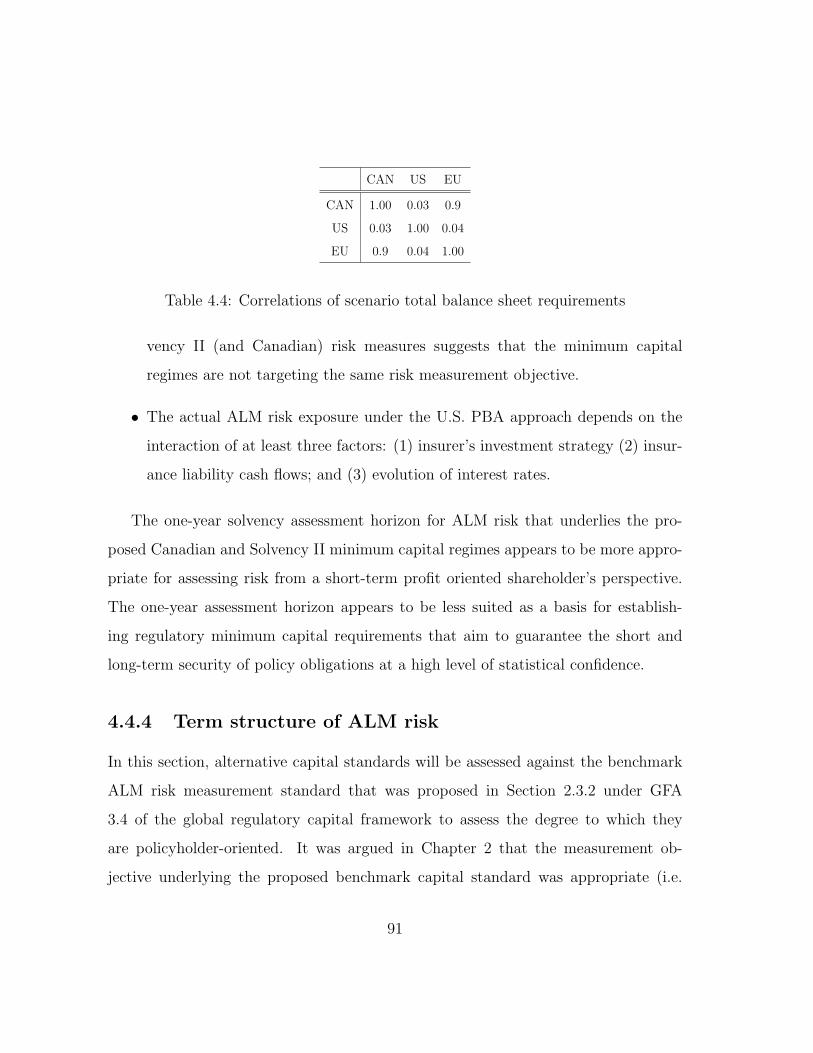
CAN US EU
CAN 1.00 0.03 0.9
US 0.03 1.00 0.04
EU 0.9 0.04 1.00
Table 4.4: Correlations of scenario total balance sheet requirements
vency II (and Canadian) risk measures suggests that the minimum capital
regimes are not targeting the same risk measurement objective.
• The actual ALM risk exposure under the U.S. PBA approach depends on the
interaction of at least three factors: (1) insurer’s investment strategy (2) insur-
ance liability cash flows; and (3) evolution of interest rates.
The one-year solvency assessment horizon for ALM risk that underlies the pro-
posed Canadian and Solvency II minimum capital regimes appears to be more appro-
priate for assessing risk from a short-term profit oriented shareholder’s perspective.
The one-year assessment horizon appears to be less suited as a basis for establish-
ing regulatory minimum capital requirements that aim to guarantee the short and
long-term security of policy obligations at a high level of statistical confidence.
4.4.4 Term structure of ALM risk
In this section, alternative capital standards will be assessed against the benchmark
ALM risk measurement standard that was proposed in Section 2.3.2 under GFA
3.4 of the global regulatory capital framework to assess the degree to which they
are policyholder-oriented. It was argued in Chapter 2 that the measurement ob-
jective underlying the proposed benchmark capital standard was appropriate (i.e.
91
policyholder-oriented) given the goal of prudential regulation.
The relevant risky scenario set of the proposed benchmark capital standard Ω′′(α, θ)
given a confidence-level α and investment or risk management strategy θ is formally
defined in Equation (4.4).
Ω′′(α, θ) = ω : ST (ω, θ) ≥ VaRα(ST (ω, θ)) (4.4)
where ST is the aggregate loss-random variable that underlies the benchmark
capital standard that is defined in Equation (2.13).
The results of Section 4.4.3 showed that the worst-case or risky scenario set
for some confidence-level α, i.e. Ω′i(α)=ω : STBSRi(ω) >= VaRα(STBSRi); i =
CAN,US,EU, at least depends on the length of the calibration period that under-
lies the capital standard. Based on the analysis of that section, the proposed Solvency
II and Canadian capital standards were shown to be not policyholder-oriented. That
is, Ω′CAN(α, θ) and Ω′
EU(α, θ) were shown to be significantly different from Ω′′(α, θ).
It is worthwhile to consider whether capital requirements can be policyholder-
oriented when the underlying risk measure is based on a calibration horizon that is
less than the full-term of the liabilities. To investigate that possibility, capital amounts
TBSRXnY R corresponding to the XnYR solvency capital rules that were introduced
in Section 2.2.3 are defined here in Equation (4.5). For notational convenience, we
denote the benchmark capital standard by X20YR. This notation is appropriate since
in the case of the term life insurance portfolio that was described in Section 4.2, the
full-term of the liability cash flows is 20 years.
92
STBSRXnY R(ω|Θ) = infx ∈ R : ALRt >= 1 ∀t = 1, .., n|Θ, ω ∈ Ω (4.5)
TBSRXnY R(Θ) = CTEα(STBSRXnY R(ω|Θ))
where n is the term of the risk measure and α = 0.9 is the desired confidence-level.
For example, the STBSRX5Y R is the amount needed to discharge policyholder obliga-
tions and also maintain the market-value based leverage-ratio (ALRt=MVAt/MVLt;
t=1,2,..,5) above 1 over a five-year calibration horizon. As explained before, the
proposed Canadian capital standard is equivalent to a X1YR solvency capital rule.
In Figures 4.6 and 4.7, risk profiles of the six investment strategies that were
described in Section 4.2 (i.e. laddered (LADD), bullet (BULL), barbell (BARB),
long bond (LB), short bond (SB) and duration matching (MATCH)) are provided as
a basis for a comparison of the alternative capital standards.
In particular, the box plots represent the (sampling) distributions of the scenario
total balance sheet requirement amount for each given capital standard. Given the
apparent lack of correlation that was observed between the proposed one-year based
capital standards (i.e. in Canada and the EU) and the longer-term U.S. PBA stan-
dard, in Sections 4.4.3 and 4.4.4, it is not surprising that the corresponding risk
profiles of the investment strategies are significantly different. The capital require-
ments for each investment strategy that have been determined in accordance with
the proposed capital standards are summarized in Table 4.5. The capital amounts
are shown as percentages of the Solvency II best-estimate liability.
A preliminary assessment of the degree to which a given capital standard is
policyholder-oriented, in terms of whether it is measuring the same underlying tail-
risk as the benchmark X20YR standard, can be made by observing the following from
Figures 4.6, 4.7 and Table 4.5:
93
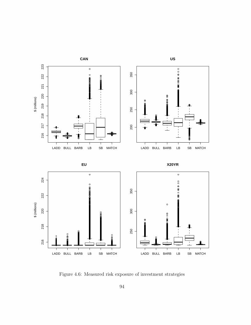
LADD BULL BARB LB SB MATCH
216
217
218
219
220
221
222
223
CAN
$ (m
illio
ns)
LADD BULL BARB LB SB MATCH
200
250
300
350
US
LADD BULL BARB LB SB MATCH
216
218
220
222
224
EU
$ (m
illio
ns)
LADD BULL BARB LB SB MATCH
250
300
350
X20YR
Figure 4.6: Measured risk exposure of investment strategies
94
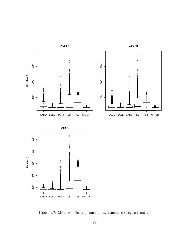
LADD BULL BARB LB SB MATCH
250
300
350
X15YR
$ (m
illio
ns)
LADD BULL BARB LB SB MATCH
250
300
350
X10YR
LADD BULL BARB LB SB MATCH
220
240
260
280
300
X5YR
$ (m
illio
ns)
Figure 4.7: Measured risk exposure of investment strategies (cont’d)
95
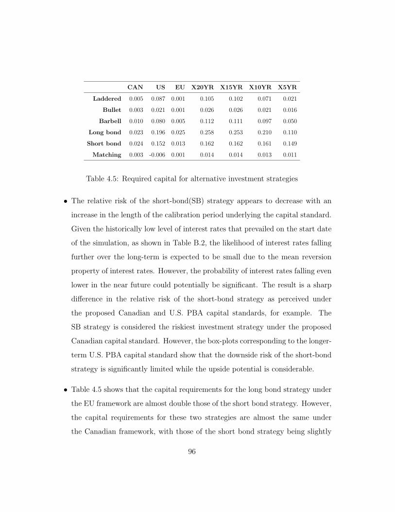
CAN US EU X20YR X15YR X10YR X5YR
Laddered 0.005 0.087 0.001 0.105 0.102 0.071 0.021
Bullet 0.003 0.021 0.001 0.026 0.026 0.021 0.016
Barbell 0.010 0.080 0.005 0.112 0.111 0.097 0.050
Long bond 0.023 0.196 0.025 0.258 0.253 0.210 0.110
Short bond 0.024 0.152 0.013 0.162 0.162 0.161 0.149
Matching 0.003 -0.006 0.001 0.014 0.014 0.013 0.011
Table 4.5: Required capital for alternative investment strategies
• The relative risk of the short-bond(SB) strategy appears to decrease with an
increase in the length of the calibration period underlying the capital standard.
Given the historically low level of interest rates that prevailed on the start date
of the simulation, as shown in Table B.2, the likelihood of interest rates falling
further over the long-term is expected to be small due to the mean reversion
property of interest rates. However, the probability of interest rates falling even
lower in the near future could potentially be significant. The result is a sharp
difference in the relative risk of the short-bond strategy as perceived under
the proposed Canadian and U.S. PBA capital standards, for example. The
SB strategy is considered the riskiest investment strategy under the proposed
Canadian capital standard. However, the box-plots corresponding to the longer-
term U.S. PBA capital standard show that the downside risk of the short-bond
strategy is significantly limited while the upside potential is considerable.
• Table 4.5 shows that the capital requirements for the long bond strategy under
the EU framework are almost double those of the short bond strategy. However,
the capital requirements for these two strategies are almost the same under
the Canadian framework, with those of the short bond strategy being slightly
96
greater. The primary reason for this difference is the assessment of incremental
capital on free assets under Solvency II as was explained in Section 4.4.1. The
distorting impact of this aspect of Solvency II in risk assessment is therefore
evident.
• The relative risk ranking of the laddered, barbell and bullet strategies under the
U.S., Canadian and EU frameworks is also of interest. The duration and con-
vexity risk measures of the initial portfolios of these strategies were summarised
in Table 4.1. Under the Solvency II capital standard, the risk of the laddered
and bullet strategies is the same, while that of the barbell is about five times
that of either the bullet or laddered strategies. Under the proposed Canadian
capital standard, the risk of the laddered strategy is about 67% greater than
that of the bullet strategy, while the risk of the barbell strategy is more than
300% that of the bullet strategy. Of the three strategies, the Canadian and EU
standards are consistent in their ranking of the barbell strategy as the riskiest.
This is in contrast to the risk assessment under the U.S. PBA standard which
ranks the laddered portfolio strategy as having the greatest risk exposure to in-
terest rate risk among the three investment strategies, with the barbell strategy
ranking second.
• As evidenced by the capital requirements in Table 4.1, the longer horizon X-
measurement methods (i.e 10, 15, and 20 year methods) are more or less con-
sistent with the U.S. framework in their relative risk rankings of the investment
portfolio strategies. The minor exception is the relative ranking of the laddered
and barbell strategies which is reversed. However, when the actual order of
magnitude of the difference in capital requirements is taken into account, this
97
inconsistency does not appear to be very material. On the other hand, the
only consistency between the rankings that are based on the five-year horizon
X5YR method and the U.S. rankings is the ranking of the bullet and duration
matching strategies as the second least and least risky strategies respectively.
• With the exception of the duration matching strategy, the capital requirements
for all other investment strategies determined under the U.S. capital framework
appear to be significantly more conservative than the corresponding require-
ments under the Canadian and Solvency II regimes. The capital requirement
for the duration matching strategy under the U.S. framework is -0.6% of the best
estimate liability since the total balance sheet requirement under that strategy
is less than the amount of the Solvency II best estimate liability. This is pos-
sible since we have not imposed the Solvency II best-estimate liability floor on
TBSRUS in Equation 4.2.
• The significantly different character of the risk exposures underlying the six in-
vestment strategies in Figures 4.6 and 4.7 highlights the challenge of implement-
ing a standard factor-based capital formula that is able to reasonably capture
the essential features of each unique exposure, as was explained in Chapter 1.
To further establish whether capital requirements under a given standard are
policyholder-oriented, the tail-dependency of a given alternative capital standard
with the benchmark standard can be analyzed. In Figure 4.8, the 100 worst-case
scenarios of the long-bond strategy in terms of the benchmark capital standard are
plotted against corresponding outcomes of each given capital standard for those same
scenarios. That is, given ω ∈ Ω′′(α = .01, θ = LB), F1 is the empirical distribution of
STBSRX20Y R(θ = LB), Fi is the empirical distribution of STBSRi(θ = LB) for a given
98
capital standard i, the tail-dependency plots in Figure 4.8 are plots of points of the
form (x,y), where x=F1(STBSRX20Y R(ω, θ = LB)) and y= Fi(STBSRi(ω, θ = LB)).
A plot which shows a strong linear relationship (note that the line x=y is indicated
by a black dotted line in each plot) such as that for the X15YR method suggests that
the given capital standard is policyholder-oriented. The tail-dependency plots of the
short-bond investment strategy are also shown in Figure 4.9 for comparison.
An analysis of Figures 4.8 and 4.9 leads to the following conclusions:
• Figures 4.8 and 4.9 show that a significant number of interest rate scenarios that
are classified as adverse (i.e. the worst 1%) under the benchmark capital stan-
dard are actually considered the least risky from the perspective of the proposed
Canadian and EU capital standards since they correspond to the minimum tar-
get capital requirement 2 under those standards. Similarly to previous results,
the proposed Canadian and EU capital adequacy standards are therefore not
policyholder-oriented.
• The graphs also suggest that the tail-dependency between an alternative capital
standard and the benchmark standard increases with the calibration horizon
underlying the alternative standard. In the case of the long-bond investment
strategy, for example, Figure 4.4 shows that the use of a time period such
as 5-years to determine regulatory capital would result in the exclusion of the
continued adverse development of interest scenarios and the investment strategy
beyond the 5-year period. For each given adverse scenario in Figure 4.4, interest
rates continue to increase beyond the 5-year calibration period, resulting in
more assets being sold at even more depressed levels to fund net payouts to
2The minimum target capital requirement under the Canadian and EU standards correspond to
a probability mass point at the amount of the best estimate liability at time t = 0.
99
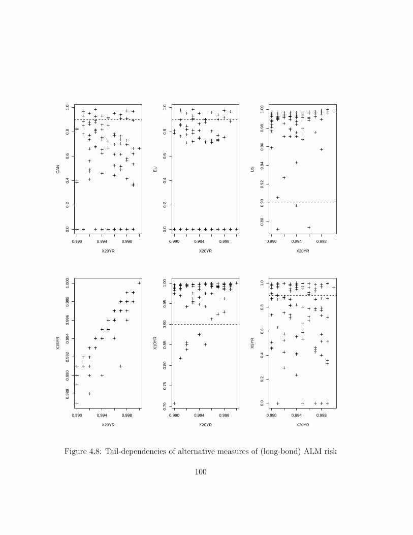
0.990 0.994 0.998
0.0
0.2
0.4
0.6
0.8
1.0
X20YR
CA
N
0.990 0.994 0.998
0.0
0.2
0.4
0.6
0.8
1.0
X20YR
EU
0.990 0.994 0.998
0.88
0.90
0.92
0.94
0.96
0.98
1.00
X20YRU
S
0.990 0.994 0.998
0.98
80.
990
0.99
20.
994
0.99
60.
998
1.00
0
X20YR
X15
YR
0.990 0.994 0.998
0.70
0.75
0.80
0.85
0.90
0.95
1.00
X20YR
X10
YR
0.990 0.994 0.998
0.0
0.2
0.4
0.6
0.8
1.0
X20YR
X5Y
R
Figure 4.8: Tail-dependencies of alternative measures of (long-bond) ALM risk
100
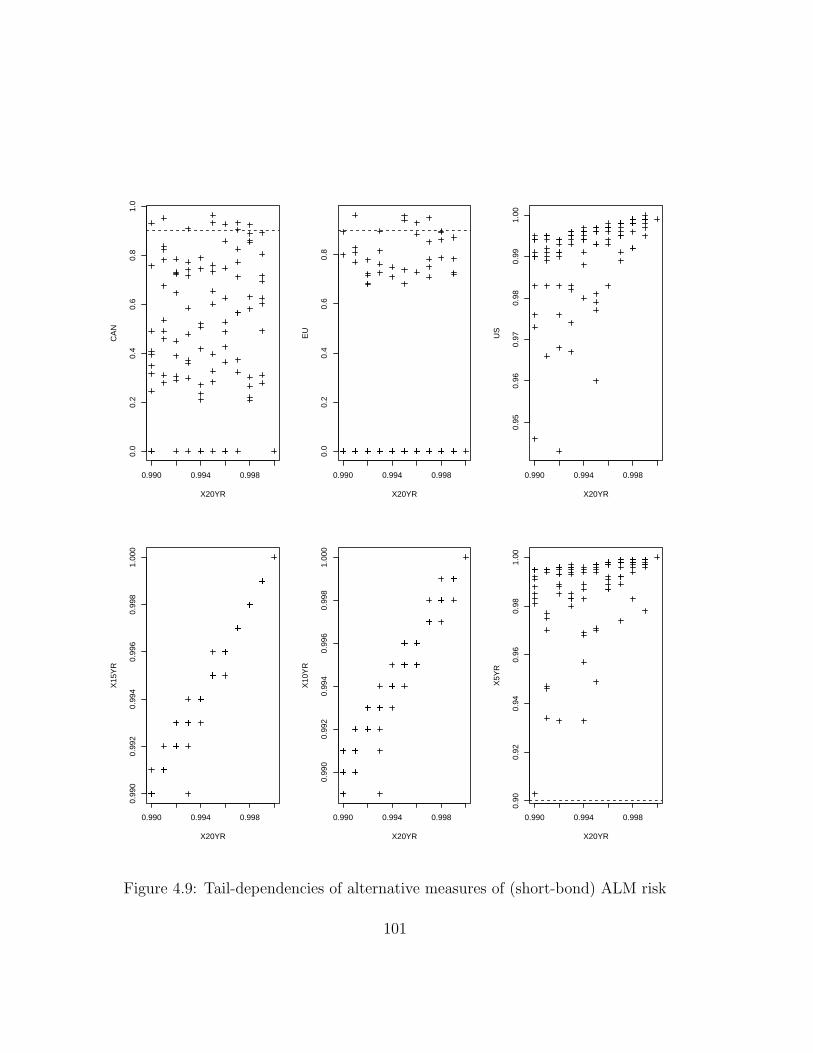
0.990 0.994 0.998
0.0
0.2
0.4
0.6
0.8
1.0
X20YR
CA
N
0.990 0.994 0.998
0.0
0.2
0.4
0.6
0.8
X20YR
EU
0.990 0.994 0.998
0.95
0.96
0.97
0.98
0.99
1.00
X20YRU
S
0.990 0.994 0.998
0.99
00.
992
0.99
40.
996
0.99
81.
000
X20YR
X15
YR
0.990 0.994 0.998
0.99
00.
992
0.99
40.
996
0.99
81.
000
X20YR
X10
YR
0.990 0.994 0.998
0.90
0.92
0.94
0.96
0.98
1.00
X20YR
X5Y
R
Figure 4.9: Tail-dependencies of alternative measures of (short-bond) ALM risk
101
insurance policyholders. Consequently, a 5-year calibration horizon is too short
to adequately capture the complete tail-risk profile of the long-bond strategy.
The X5YR-based capital requirement is therefore not policyholder-oriented in
the case of the long bond strategy because of its low tail-risk correlation with
the benchmark capital standard which reflects all material risk over the term
of the liabilities. However, Figure 4.8 suggests that a 15-year period might be
adequate. Conversely, the tail-dependency plots of the short-bond strategy in
Figure 4.9 show that a 5-year horizon is likely adequate to completely describe
the long-term risk profile of this strategy. The same figure suggests that a 10-
year calibration period will result in an extremely good proxy for the benchmark
capital standard. Relative to the long-bond strategy, the risk of the short-
bond strategy appears to be front-loaded, therefore allowing shorter calibration
periods to be used.
• In Section 2.2.4, a method to decompose the ALM risk exposure of a given
investment or risk management strategy by future time period, as measured
under the benchmark capital standard, was suggested by Equation 2.8. In or-
der to better understand the tail-dependency plots in Figures 4.8 and 4.9, we
can make use of the term structure decomposition of the ALM risk exposures of
the long and short-bond investment strategies. The ALM risk term structures
corresponding to these strategies are respectively depicted in Figures 4.10 and
4.11. An analysis of Figure 4.10 shows that only 2% of the long-bond strategy’s
risk is due to exposure in the first period. The cumulative percentages of the
long-bond’s total ALM risk exposure that can be explained at the end of the
fifth, tenth, and fifteenth years are respectively 26%, 74% and 98%. Given this
risk decomposition, it is relatively easy to explain the observed tail-correlations
102
in Figure 4.8. For example, the observed low tail-correlations of the proposed
Canadian and Solvency II capital standards with the proposed benchmark capi-
tal standard are due to the fact the one-year based standards are only capturing
about 2% of the total ALM risk exposure of the long-bond strategy. The term
structure decomposition of the ALM risk exposure of the short-bond strategy
that is shown in Figure 4.11 reveals a different picture. By the end of the fifth
year, about 90% of the total ALM risk has already been explained. This ob-
servation confirms the earlier conclusion that was reached in the examination
of the tail-dependency plots that the X5YR capital standard was probably ad-
equate or policyholder-oriented in terms of analyzing the risk of the short-bond
strategy. The combined use of the benchmark capital standard that has been
proposed in this thesis and the associated term structure decomposition of capi-
tal that is described by Equation 2.8, thus appears to be an immensely powerful
and more complete tool for describing the insurer’s ALM risk exposure given
an underlying investment or risk management strategy.
In conclusion, the analysis of this section has shown us that a capital standard
need not use a calibration horizon that extends to the full-term of the liabilities in
order to be considered policyholder-oriented, in the sense that was defined in Chapter
2. A shorter calibration horizon is possible if the term structure decomposition of the
benchmark ALM risk exposure indicates that a significant percentage of the risk is
explained within that measurement period.
103
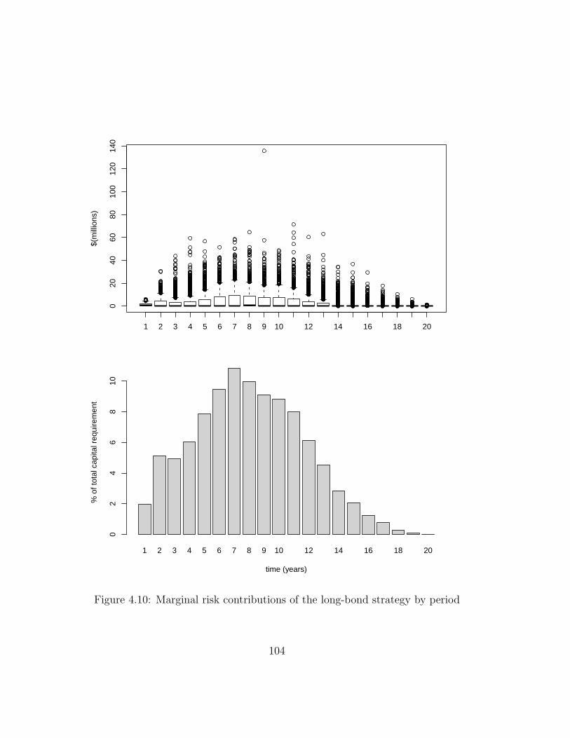
1 2 3 4 5 6 7 8 9 10 12 14 16 18 20
020
4060
8010
012
014
0
$(m
illio
ns)
1 2 3 4 5 6 7 8 9 10 12 14 16 18 20
time (years)
% o
f tot
al c
apita
l req
uire
men
t
02
46
810
Figure 4.10: Marginal risk contributions of the long-bond strategy by period
104
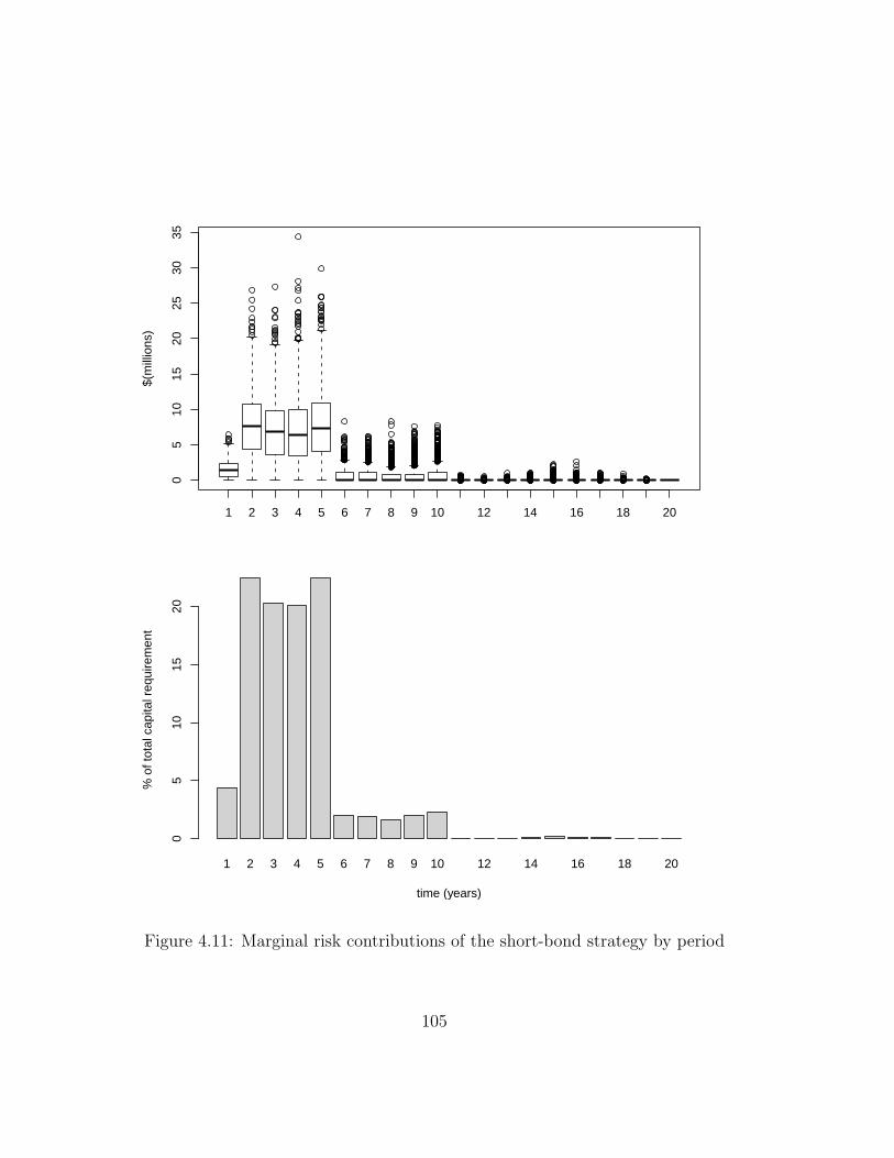
1 2 3 4 5 6 7 8 9 10 12 14 16 18 20
05
1015
2025
3035
$(m
illio
ns)
1 2 3 4 5 6 7 8 9 10 12 14 16 18 20
time (years)
% o
f tot
al c
apita
l req
uire
men
t
05
1015
20
Figure 4.11: Marginal risk contributions of the short-bond strategy by period
105

4.4.5 An incentive-based review of proposed capital stan-
dards
In the three-pillar solvency regulation framework, it has been argued throughout this
thesis that the pillar 1 capital requirements should be designed and calibrated such
that the resulting incentive structure of the capital requirements is appropriate from
a prudential regulation perspective. Studies by Kim and Santomero (1988); Rochet
(1992) conclude that poorly designed capital requirements can create incentives for
regulatory arbitrage by banks. Accordingly, GFA 3.3 requires a capital framework to
be cognisant of the economic incentives that it creates.
The behavioral incentives that are implied by a given capital standard will be
analyzed in this section using notation that was introduced in Section 2.2.5. The
corresponding incentives for each of the proposed Canadian FIMA, US PBA, Solvency
II and benchmark capital standards are shown in Table 4.6. For a given capital
standard l, each element of the incentive matrix corresponds to the quantity Γl(θi,θj)
which is defined by Equation (4.6). It measures the capital savings in percentage
terms when the insurer changes its investment strategy from θi to θj.
Γ(θi, θj) =I(θi, θj)
I(θi)(4.6)
where I(θi,θj) is as defined in Equation (2.9). That is, I(θi,θj) is the dollar amount
of capital savings when the insurer changes its investment strategy from θi to θj, where
i and j are the row and column indicators of the incentive matrix. I(θi) is simply the
amount of regulatory capital for investment strategy θi that is indicated in Table 4.5.
As previously defined, a system of incentives will considered to be policyholder-
oriented if it is largely consistent with the incentive structure of the benchmark capital
106

standard (i.e. ΓBM(θi,θj)). Policyholder-oriented incentives are designed to encour-
age insurer behaviour that is consistent with the overall goal of prudential supervi-
sion, which is to ensure the complete and timely discharge of existing policyholder
obligations. Accordingly, if the incentive matrix of a given capital standard is incon-
sistent with the benchmark incentives, we can conclude that the insurer’s sharehold-
ers/management are being encouraged to engage in risk-taking behavior that is not
completely aligned with the overall objective of prudential regulation.
An examination of Table 4.6 shows that the incentive structures implied by the pro-
posed capital standards, with the exception of the proposed US PBA, are significantly
different from those of the benchmark standard. Therefore, the proposed Solvency II
and Canadian capital standards do not necessarily result in incentives that encourage
prudent risk management from a policyholder or regulatory perspective.
The percentage capital savings when an insurer changes from a long-bond (θ5)
to a short-bond investment strategy (θ4) are ordered as follows: (ΓEU = 0.5) >
(ΓBM = 0.4) > (ΓUS = 0.2) > (ΓCAN = 0.0). The Solvency II capital standard
therefore offers the greatest incentive for this portfolio change while the proposed
Canadian standard does not offer any incentive at all. This sharp difference between
the one-year based Canadian and Solvency II capital standards is an example of the
potential distortion in risk assessment that results from the determination of capital
on free assets under Solvency II. From the viewpoint of prudential regulation, the
change to a short bond strategy is a favorable move that should be encouraged (since
ΓBM=0.4). In terms of all the capital standards in Table 4.6, the matching strategy
(θ6) is considered the least risky. Consequently, an insurer would expect non-negative
capital savings if it were to adopt this derisking strategy. The degree to which the
107
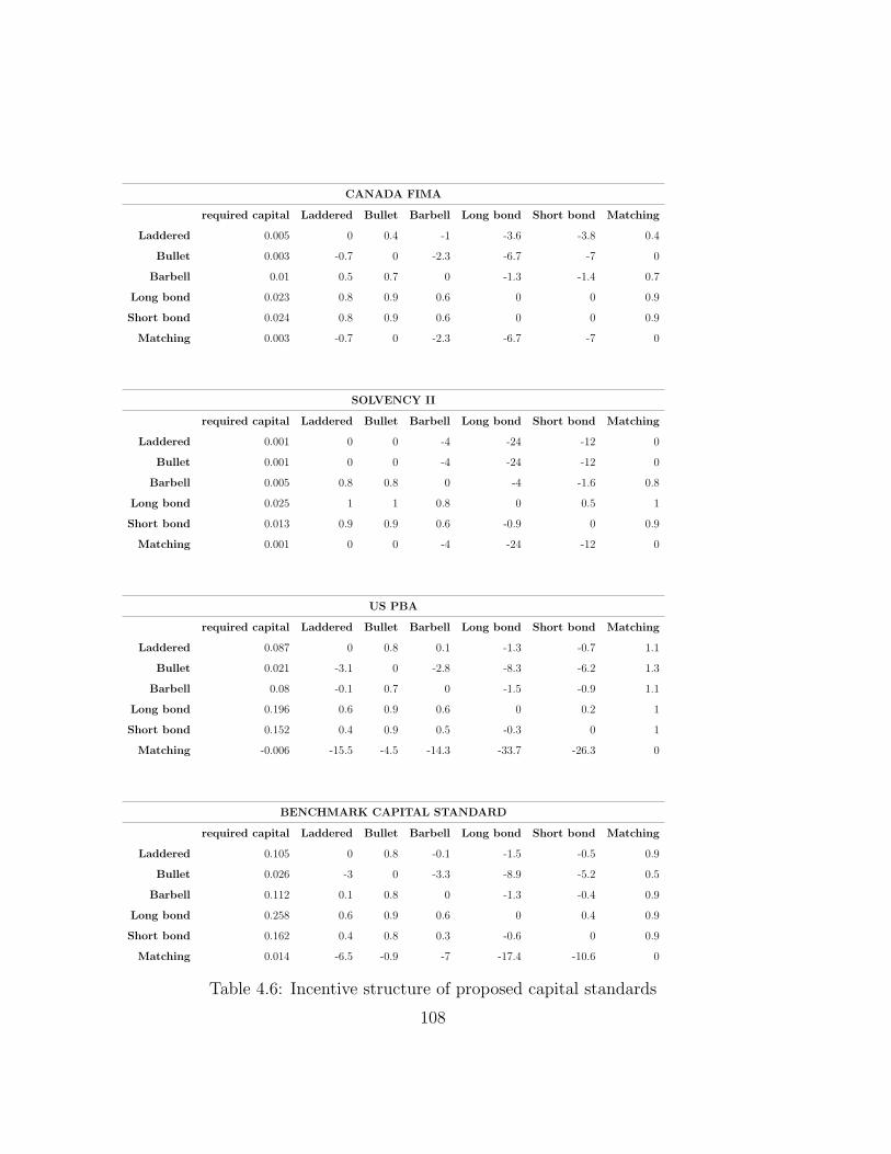
CANADA FIMA
required capital Laddered Bullet Barbell Long bond Short bond Matching
Laddered 0.005 0 0.4 -1 -3.6 -3.8 0.4
Bullet 0.003 -0.7 0 -2.3 -6.7 -7 0
Barbell 0.01 0.5 0.7 0 -1.3 -1.4 0.7
Long bond 0.023 0.8 0.9 0.6 0 0 0.9
Short bond 0.024 0.8 0.9 0.6 0 0 0.9
Matching 0.003 -0.7 0 -2.3 -6.7 -7 0
SOLVENCY II
required capital Laddered Bullet Barbell Long bond Short bond Matching
Laddered 0.001 0 0 -4 -24 -12 0
Bullet 0.001 0 0 -4 -24 -12 0
Barbell 0.005 0.8 0.8 0 -4 -1.6 0.8
Long bond 0.025 1 1 0.8 0 0.5 1
Short bond 0.013 0.9 0.9 0.6 -0.9 0 0.9
Matching 0.001 0 0 -4 -24 -12 0
US PBA
required capital Laddered Bullet Barbell Long bond Short bond Matching
Laddered 0.087 0 0.8 0.1 -1.3 -0.7 1.1
Bullet 0.021 -3.1 0 -2.8 -8.3 -6.2 1.3
Barbell 0.08 -0.1 0.7 0 -1.5 -0.9 1.1
Long bond 0.196 0.6 0.9 0.6 0 0.2 1
Short bond 0.152 0.4 0.9 0.5 -0.3 0 1
Matching -0.006 -15.5 -4.5 -14.3 -33.7 -26.3 0
BENCHMARK CAPITAL STANDARD
required capital Laddered Bullet Barbell Long bond Short bond Matching
Laddered 0.105 0 0.8 -0.1 -1.5 -0.5 0.9
Bullet 0.026 -3 0 -3.3 -8.9 -5.2 0.5
Barbell 0.112 0.1 0.8 0 -1.3 -0.4 0.9
Long bond 0.258 0.6 0.9 0.6 0 0.4 0.9
Short bond 0.162 0.4 0.8 0.3 -0.6 0 0.9
Matching 0.014 -6.5 -0.9 -7 -17.4 -10.6 0
Table 4.6: Incentive structure of proposed capital standards
108
matching strategy is incentivized under each capital standard follows the general
pattern: ΓUS > ΓBM > ΓCAN > ΓEU .
Lastly, as general rule, capital standards that are based on a short-term calibration
horizon can be expected to encourage a short-term perspective to risk assessment by
the shareholders of the insurer.
4.5 The impact of model risk on relative risk and
capital assessments
In Chapter 2, GFA 3.2 of the global capital framework requires the capital require-
ments to be optimally risk-sensitive from the policyholder’s perspective, as defined in
Section 2.3.2 of that chapter. In other words, the capital requirements must satisfy
the following two conditions:
1. They must be policyholder-oriented as discussed in the preceding sections.
2. They should be structured such that they are not prone to significant measure-
ment error that can distort risk measurements.
Three types of measurement error (εA, εL and εCF ) that should be considered in
the design and calibration of the capital framework were discussed in Section 2.3.2.
It was noted in that section that the relative magnitude of the errors depended on
the nature of the asset and liability portfolios. In particular, all three errors can be
expected to be large when the asset and liability portfolios contain complex guarantees
and embedded options that are difficult to model and value.
The implementation of the general framework for assessing the market value of
insurance liabilities that was outlined Section 2.2.2 is challenging. The valuation error
109
for typically illiquid insurance liabilities εL can therefore be potentially significant and
this should be a consideration in the final design and calibration of the corresponding
regulatory capital requirements.
The potential impact of the Type C (scenario generator) model error on the deter-
mination of US PBA capital requirements will be illustrated in the case of the short
bond strategy in this section. Under the short bond strategy, the entire portfolio is
invested in five-year risk-free coupon bonds as described in Section 4.2. Whenever the
bonds in the portfolio mature, the proceeds are rolled over into new five-year bonds.
The uncertainty of interest rates at the times when new bonds have to be purchased
is the primary source of the investment risk of the short bond strategy.
Reinvestment risk is an important consideration in the many insurance markets
where the universe of available investment instruments is not of sufficient duration to
match that of the liabilities. Zero-coupon swaps or notes, long-dated cross currency
swaps and inverse floaters are among the tools that can be used to hedge reinvestment
risk in such markets provided the infrastructure to use such hedging techniques is
sufficiently developed. Swaption strategies can also be used to allow the insurer the
opportunity to capitalize on favorable movements in interest rates.
The top graph in Figure 4.12 shows the risky (‘worst case’) interest rate scenario
set for the short bond strategy in terms of the U.S. PBA capital framework.
As can be identified in Figure 4.12, the risky scenario set is characterized by low
interest (reinvestment) rates at time horizons of 5, 10 and 15 years, when the insurer’s
investment portfolio is rolled over into new five-year bonds.
It was noted in Figures 4.6 and 4.7 that the relative risk of the short bond strategy
appeared to be much greater when a shorter horizon was used to measure the risk.
Figure 4.12 reflects the expectation that is embedded in the 10,000 interest rate
110

0 5 10 15 20
0.02
0.03
0.04
0.05
0.06
0.07
0.08
Rat
e
Percentiles
95%
50%
10%
5%
1%
Sample distribution of 5−year interest rates (10,000 scenarios)
0 5 10 15 20
0.01
00.
020
0.03
00.
040
time (years)
Rat
e
Worst 5−year interest rate scenarios
Figure 4.12: Reinvestment risk of the short bond strategy
111
scenarios that were used in the simulation that five-year interest rates will tend to
increase with time. Further, given that the starting interest rates in the simulation
were very low and because of the mean reversion property of interest rates, Figure 4.12
shows that the downside risk in terms of interest rates falling further is significantly
limited over the long-haul. However, it is likely that interest rates will fall further in
the short-term. These underlying “views” on the short and long-term paths of future
interest rates that are embedded in the scenario generator model largely contribute
to the conflicting relative risk assessments of the short bond strategy versus the long
bond or barbell strategy (as shown in Figures 4.6 and 4.7), for example. In particular,
given the view that interest rates are much more likely to rise than fall over the long-
term, Figure 4.6 suggests that the downside risk of the short bond strategy is limited
while the upside potential is significant. The determination of capital and assessment
of risk under the U.S. cash-flow based capital standard is therefore potentially exposed
to significant model error. To the extent that the scenario generator model has
been misspecified, the corresponding risk management decisions and solvency capital
calculations will be misleading. For example, if the likelihood of reinvestment rates
being lower than current rates over the long-haul is actually much higher than that
which is embedded in the 10,000 C-3 Phase III scenarios that were used in the risk
calculations, the relative risk of the short bond strategy would be much higher than
determined in Section 4.4.5.
The potential benefit of imposing a market-based leverage constraint on a cash-
flow based capital requirement (e.g. US PBA capital framework) in terms of reducing
the impact of the subjectivity of modeling assumptions was motivated in Section 2.3.2
under GFA 3.4.
112

4.6 Chapter conclusion
A general framework for assessing the ALM-risk exposure of a life insurer has been
provided in this chapter. The recommended approach for the measurement of ALM
risk can serve as a unifying framework for the principle-based ALM-risk capital stan-
dards that have been proposed in the U.S., Canada, and the EU.
In Section 4.4.4, alternative capital standards were compared against the bench-
mark standard that has been proposed in the thesis to determine the extent to which
they are ‘policyholder-oriented’. As defined in Chapter 2, capital requirements are
policyholder-oriented if the measurement objective of the underlying risk measure re-
flects the ultimate goal of prudential supervision, the complete and timely discharge
of all existing policyholder obligations. If the calibration period that underlies a given
capital standard is such that a significant proportion of the overall ALM risk expo-
sure of the insurer is explained by exposure in that period, then the resulting capital
requirement adequately reflects the policyholders’ exposure to the default risk of the
insurer. In the analysis of Section 2.2.4, the benchmark capital standard and the
ALM risk decomposition technique that is described in Section 2.2.4 were shown to
be invaluable tools for making this determination.
Throughout the thesis, it has been stressed that the incentive effect of capital
requirements should be a primary consideration in the design and calibration of a
regulatory capital framework. For example, the decision of what, if any, incentives
should be provided through capital requirements for insurers to bulk up or diversify
is an important one. As noted in Chapter 3, the Canadian MCCSR formula does
not offer any credits for diversifying among its component risk categories. On the
other hand, as noted in that chapter, the incentives for diversification under the
Solvency II standard formula appear to be very significant. The overall consideration
113
in determining the appropriateness of incentives offered under a capital framework
depends on whether their application serves to promote the overall goal of prudential
supervision. In Section 4.4.5, a suggestive framework for analyzing and calibrating the
incentives that underly a capital standard for life insurers was presented. Essentially,
the incentive structure that is implied by a given life insurer capital standard must
be largely consistent with the incentive structure of the benchmark capital standard.
Such an incentive scheme is considered to be policyholder-oriented in the sense that
has been defined in the thesis. The design of the proposed Solvency II and Canadian
capital standards implies an incentive structure for ALM risk that is not policyholder-
oriented.
Finally, the design of a capital framework should consider the three sources of
measurement error that could distort the underlying risk measures. They are errors
in asset valuation, liability valuation, and in the cash-flow model of the assets and
liabilities (which includes sampling error). For example, measurements of capital
that are based on a short-term calibration horizon such as one year (e.g. proposed
Solvency II and Canadian capital standards) are particularly prone to errors in asset
and liability valuation. Longer-horizon based capital standards such as the US PBA
and the proposed benchmark capital standard would be more prone to errors in
cash-flow modeling than they are to valuation risk. Policyholder-oriented capital
requirements that minimize the incidence of measurement error risk are considered to
be ‘optimally’ risk sensitive. An optimally risk-sensitive regulatory capital framework
reflects the overall goal of prudential supervision in an optimal fashion, giving due
consideration to the associated challenges of implementation.
In Section 4.4.3, the apparent low correlation between the ALM-risk measurements
that underly the U.S. and the proposed Canadian and EU capital standards was
114
illustrated in the case of a twenty-year life insurance product. The one-year calibration
horizon of the Solvency II and Canadian frameworks was shown to be inadequate for
describing the ALM-risk profile of long-term strategies. An analysis of the ALM-risk
term structure of the long-bond strategy validated this conclusion since only 2% of
the strategy’s overall long-term risk could be explained by exposure in the first year.
Additionally, the inadequacy of the one-year based capital standards in measuring
long-term risk exposures implies that they cannot function as effective early warning
indicators of financially distressed insurers to insurance supervisors.
The global financial crisis of 2007-2009 highlighted the pitfalls of a short-term ori-
ented approach to the appraisal of enterprise risk that was caused, among other fac-
tors, by poorly structured managerial incentives. The troubled financial institutions
that were at the epicenter of the crisis were widely criticized for making short-term
business decisions that did not give due regard to long-term consequences. In the
context of life insurance, the work of this chapter can be applied to determine the
appropriate calibration horizon for a regulatory capital standard so that the corre-
sponding incentive structure is aligned with the single goal of prudential regulation,
the minimization of losses to policyholders due to insurer insolvency.
115
Chapter 5
Policy recommendations,
applications of thesis results and
future research
5.1 Introduction
As discussed in Chapter 1, the solvency regulation standards that are emerging in
different jurisdictions can be generally organized under three pillars – quantitative
capital requirements, supervisory review and market discipline. The use of a three-
pillar solvency regulation mechanism has the potential problem that is described by
Eling (2010) as follows, “Combining two approaches always runs the risk that a little
of everything will be done, but not enough of anything (just like the “stuck in the
middle” problem described by Porter (1980))”.
In Chapter 4, significant differences were identified among the proposed Canadian,
US PBA and Solvency II capital standards with respect to the measurement of ALM
116
risk. In Chapter 2, a benchmark framework for measuring the insolvency risk of a
life insurer was proposed. This framework was then applied to the measurement of
ALM risk in Chapter 4 and was suggested as a possible basis for achieving global
convergence in solvency standards.
The goal of this chapter is to suggest changes that can be made to the proposed
Canadian, Solvency II and US PBA capital standards, as described in this thesis, in
order to bring about convergence to the proposed global benchmark standard.
5.2 Market discipline
The primary reason for subjecting insurers to solvency regulation that was provided
in Chapter 1 is based on the fact that the policyholders of an insurer are typically
not able to effectively monitor and influence the insurer in their own capacity to
protect their interest. In that same chapter, significant impediments that may exist
to render ineffective the operation of market-discipline were provided. Information
asymmetry and costly information are cited in Eling (2010) as possible impediments
to the operation of market discipline. Life insurance and annuity contracts typically
contain complex long-term guarantees and options that are extremely difficult to
analyze. This makes it difficult for market participants, including policyholders and
intermediaries such as rating agencies and brokers, to provide effective monitoring of
the insurer’s risk portfolio. Consequently, market participants generally have to rely
on the integrity of the insurer’s management for accurate disclosure of the insurer’s
risk positions. Given that dishonest or incompetent management is frequently the
reason cited for insurer failure, the ability of market participants to effectively monitor
the insurer’s insolvency risk is at best questionable.
117
The effectiveness of market-discipline can be enhanced if the insurance policyhold-
ers and other market participants are furnished with relevant and timely information
that they are able to process and act upon. Eling (2010) notes that for market
discipline to work, the information that is provided to market participants must be
“timely, standardized, consistent and transparent”. The term structure of insolvency
risk decomposition that was proposed and illustrated in Chapters 2 and 4, respec-
tively, can be provided to market participants as a pillar-three disclosure. The benefits
of including the term structure of insolvency risk in the pillar-three disclosures are:
1. It is an efficient risk summary that is particularly suited for dissemination
to market participants. It can be provided at the portfolio, business line or
enterprise-wide levels depending on the particular application.
2. It is easy to understand. The amount of capital allocated to a given period is
based on the marginal risk contribution of that period to the insurer’s overall
insolvency risk over the term of the liabilities.
3. It provides more complete information than any single number. For exam-
ple, it allows ALM strategies with risk profiles that are ‘front-loaded’ to be
distinguished from those that are “back-loaded” (similar to a ponzi-scheme).
Hirst et al. (2007) show that market participants find earnings forecasts by
management more credible when information on the component earnings by
source (i.e. income statement line items) is included in the disclosure along
with the combined earnings forecast. Accordingly, we can expect that market
participants will be more likely to act on the disaggregated risk information
that is provided by the term structure decomposition of insolvency or ALM risk
since they will find it to be more credible and informative than a single number.
118
4. It provides a context for assessing the appropriateness or relevance of shorter-
term based risk measures. For example, a short-term risk measure would be
judged to be inadequate for assessing the risk exposure of an insurer strategy
that is back-loaded since it effectively cuts off the tail of the risk profile.
In summary, providing the term structure decomposition of the insurer’s insol-
vency risk to market participants should enhance the effectiveness of pillar-three of
the solvency regulation framework. This applies whether the underlying pillar-one
capital requirements are based on the U.S. PBA, proposed Canadian or Solvency II
standards. Increased transparency in the insurer’s risk portfolio should also have the
benefit of reducing its cost of capital.
5.3 Proposed Canadian and Solvency II capital
standards
As noted in Chapter 4, the proposed Canadian and Solvency II capital standards are
not policyholder oriented. Accordingly, the incentives that are provided under these
(pillar 1) standards are not always consistent with the overall objective of prudential
regulation as discussed in Section 4.4.5 of the previous chapter. To that end, the other
pillars can be potentially used to negate the impact of the misaligned incentives.
In order of preference, the following recommendations are provided to address the
potential shortcomings of the one-year based capital standards:
1. The pillar 1 capital requirements for ALM risk should be redesigned so that
they become policyholder-oriented. It is understood that this will be a difficult
119

task to undertake at this time given the considerable progress that has been
made toward adopting Solvency II in its current form.
2. The insurer’s term structure of insolvency risk should be used as primary tool
for the conduct of the supervisory review pillar of the solvency regulation frame-
work. As a quantitative summary measure of the insurer’s overall risk exposure
with respect to existing business, it should add a lot of value to the primarily
qualitative exercises conducted under this pillar.
3. As explained in the previous section, market participants should be furnished
with information on the insurer’s term structure of risk exposures.
5.4 US PBA capital standard
The US PBA capital framework fared better than the proposed Solvency II and
Canadian capital standards in the analysis that was conducted in Chapter 4. The
absence of the market-based leverage-ratio constraint in the US PBA capital standard
is the only source of difference with the benchmark standard. The risk-management
benefits of the proposed market-based leverage constraint were explained in Section
2.3.2 under GFA 3.4. Accordingly, application of this leverage constraint should be
an improvement of the proposed US PBA capital standard for all life insurance and
annuity products.
In Table 4.5, the capital requirement for the matching strategy was found to
be negative when the market-value measure of the liability was used. Accordingly,
imposing a balance-sheet constraint that is based on market values would make the
US PBA capital standard more compatible with a market valuation balance-sheet.
The first two components of the insurance contract liability that are described in the
120
exposure draft of the IFRS insurance standard (IASB (2010)) should be reasonably
correlated with a market-value based measurement. The leverage constraint would
therefore also make the US PBA capital standard more consistent with the proposed
IFRS for insurance, which is important due to the global reach of the international
reporting standards.
5.5 Other potential applications of thesis results
Other potential applications of the results in this thesis include the following:
1. The disclosures that have been recommended in the previous section can also
be used in public financial reports.
2. The term structure decomposition can be used in portfolio selection in the case
where assets are being managed against a liability benchmark.
3. The risk decomposition technique can also be applied in the relative assessment
of economic capital and risk given alternative insurer strategies.
5.6 Conclusion and future research
The potential applications of the benchmark capital standard and its associated term
structure decomposition have been reviewed in this chapter. A possible pathway of
achieving convergence in the proposed US PBA, Canadian and Solvency II capital
standards has also been offered.
Opportunities for future research include the following:
121
1. Eling (2010) suggests there is a strong need of research to enhance our currently
limited understanding of market discipline as it applies to insurance. From a
solvency regulation standpoint, customer or insurance product-driven market
discipline should be the primary focus of these further investigations.
2. The specific analysis of the proposed U.S. PBA, Canadian and Solvency II
capital standards that was presented in Chapter 4 can be enhanced by including
the following elements in the comparison:
• Applicable minimum capital floors. For example, the Minimum Capital
Requirement (MCR) under Solvency II, the Deterministic Reserve (DR)
under the US PBA, etc.
• A numerical analysis of dynamic aspects of each capital regime. For exam-
ple, further research to evaluate the extent of the increase in the volatility
of the capital requirements under the proposed Solvency II and Canadian
standards, and to anticipate the impact of the increased volatility on the
insurer’s ALM risk practices.
3. The ALM risk measurement framework that has been proposed in this thesis
implies that the term structure decomposition of the insurer’s risk exposure
will vary with the nature of the insurer’s product portfolio and investment/risk
management. Research can be undertaken to develop guidelines for determining
the appropriate calibration period for specific insurance products and common
investment strategies.
In conclusion, the unified framework for analyzing insolvency risk and associated
capital requirements that has been presented in this thesis should be a valuable con-
122

tribution to the development of a global regulatory capital framework for life insurers.
123

Appendices
124
Appendix A
Data and formulas for Chapter 3
calculations
A.1 Model portfolio and valuation assumptions
Model insurance portfolio
• 1,000,000 identical policies issued to males aged 35
• 30-year level, non-renewal term life product
• $500,000 face amount per policy
• Premium rate of $2 per $1,000 face amount
Interest rates
The interest rates that were used in the calculations are shown in Table A.1.
125
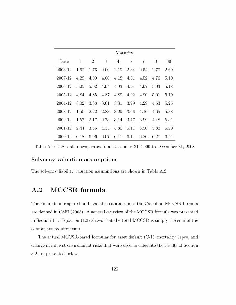
Maturity
Date 1 2 3 4 5 7 10 30
2008-12 1.62 1.76 2.00 2.19 2.34 2.54 2.70 2.69
2007-12 4.29 4.00 4.06 4.18 4.31 4.52 4.76 5.10
2006-12 5.25 5.02 4.94 4.93 4.94 4.97 5.03 5.18
2005-12 4.84 4.85 4.87 4.89 4.92 4.96 5.01 5.19
2004-12 3.02 3.38 3.61 3.81 3.99 4.29 4.63 5.25
2003-12 1.50 2.22 2.83 3.29 3.66 4.16 4.65 5.38
2002-12 1.57 2.17 2.73 3.14 3.47 3.99 4.48 5.31
2001-12 2.44 3.56 4.33 4.80 5.11 5.50 5.82 6.20
2000-12 6.18 6.06 6.07 6.11 6.14 6.20 6.27 6.41
Table A.1: U.S. dollar swap rates from December 31, 2000 to December 31, 2008
Solvency valuation assumptions
The solvency liability valuation assumptions are shown in Table A.2.
A.2 MCCSR formula
The amounts of required and available capital under the Canadian MCCSR formula
are defined in OSFI (2008). A general overview of the MCCSR formula was presented
in Section 1.1. Equation (1.3) shows that the total MCCSR is simply the sum of the
component requirements.
The actual MCCSR-based formulas for asset default (C-1), mortality, lapse, and
change in interest environment risks that were used to calculate the results of Section
3.2 are presented below.
126
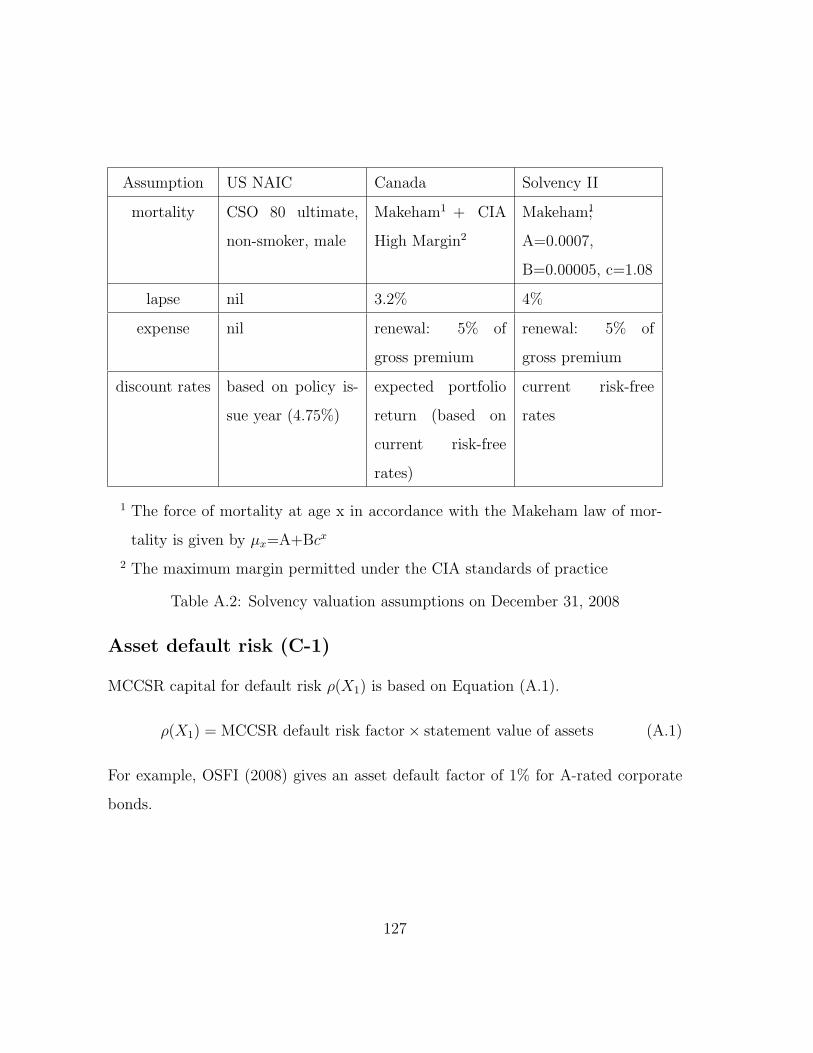
Assumption US NAIC Canada Solvency II
mortality CSO 80 ultimate,
non-smoker, male
Makeham1 + CIA
High Margin2
Makeham1;
A=0.0007,
B=0.00005, c=1.08
lapse nil 3.2% 4%
expense nil renewal: 5% of
gross premium
renewal: 5% of
gross premium
discount rates based on policy is-
sue year (4.75%)
expected portfolio
return (based on
current risk-free
rates)
current risk-free
rates
1 The force of mortality at age x in accordance with the Makeham law of mor-
tality is given by µx=A+Bcx
2 The maximum margin permitted under the CIA standards of practice
Table A.2: Solvency valuation assumptions on December 31, 2008
Asset default risk (C-1)
MCCSR capital for default risk ρ(X1) is based on Equation (A.1).
ρ(X1) = MCCSR default risk factor× statement value of assets (A.1)
For example, OSFI (2008) gives an asset default factor of 1% for A-rated corporate
bonds.
127

Mortality risk
Equation (A.2) gives overall mortality risk ρ(X2,m) as the sum of the volatility and
catastrophic risk components, which are respectively defined by Equation (A.3) and
Equation (A.4).
ρ(X2,m) = volatility risk component + catastrophic risk component (A.2)
with
volatility risk component = 2.5× A× B× E/F (A.3)
where:
• A is the standard deviation of the projected death claims in the year immedi-
ately following the valuation date.
It is calculated by the following formula:
A =
√ ∑allpolicies
q(1− q)b2
where q is the valuation mortality and b is the death benefit for the policy.
• B is defined as follows:
B = max (1, lnD)
where D is the Macaulay Duration of the projected net death claims for the
term-life insurance portfolio at a discount rate of 5%
• E is the total net amount at risk for the term-life portfolio
128

• F is the total face amount
catastrophic risk capital = α× C× E/F (A.4)
where:
• α = 10%
• C is next year’s expected death claims
• E is the total net amount at risk
• F is the total face amount of insurance
Lapse risk
MCCSR capital for lapse risk ρ(X2,l) is based on Equation (A.5).
ρ(X2,l) = CALM reserveA − CALM reserveB (A.5)
where:
• CALM reserveA is the CALM reserve for the term insurance portfolio that has
been calculated using appropriate valuation assumptions.
• CALM reserveB is the CALM reserve that has been recalculated using a more
conservative lapse assumption i.e. an additional 15% margin to that already
assumed in the valuation. For example if a 10% margin had already been
assumed in the valuation, ReserveB will be based on a lapse margin assumption
of 10% + 15% = 25%.
129
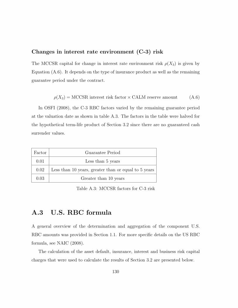
Changes in interest rate environment (C-3) risk
The MCCSR capital for change in interest rate environment risk ρ(X3) is given by
Equation (A.6). It depends on the type of insurance product as well as the remaining
guarantee period under the contract.
ρ(X3) = MCCSR interest risk factor× CALM reserve amount (A.6)
In OSFI (2008), the C-3 RBC factors varied by the remaining guarantee period
at the valuation date as shown in table A.3. The factors in the table were halved for
the hypothetical term-life product of Section 3.2 since there are no guaranteed cash
surrender values.
Factor Guarantee Period
0.01 Less than 5 years
0.02 Less than 10 years, greater than or equal to 5 years
0.03 Greater than 10 years
Table A.3: MCCSR factors for C-3 risk
A.3 U.S. RBC formula
A general overview of the determination and aggregation of the component U.S.
RBC amounts was provided in Section 1.1. For more specific details on the US RBC
formula, see NAIC (2008).
The calculation of the asset default, insurance, interest and business risk capital
charges that were used to calculate the results of Section 3.2 are presented below.
130
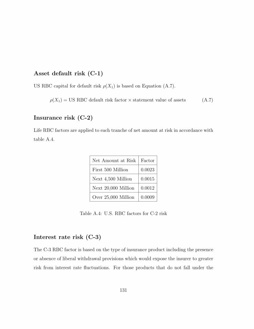
Asset default risk (C-1)
US RBC capital for default risk ρ(X1) is based on Equation (A.7).
ρ(X1) = US RBC default risk factor× statement value of assets (A.7)
Insurance risk (C-2)
Life RBC factors are applied to each tranche of net amount at risk in accordance with
table A.4.
Net Amount at Risk Factor
First 500 Million 0.0023
Next 4,500 Million 0.0015
Next 20,000 Million 0.0012
Over 25,000 Million 0.0009
Table A.4: U.S. RBC factors for C-2 risk
Interest rate risk (C-3)
The C-3 RBC factor is based on the type of insurance product including the presence
or absence of liberal withdrawal provisions which would expose the insurer to greater
risk from interest rate fluctuations. For those products that do not fall under the
131

scope of C-3 Phase I and C-3 Phase II, the C-3 risk capital requirements ρ(X3) are
generally determined by Equation (A.8).
ρ(X3) = US RBC factor for C-3 risk× formula-based reserves (A.8)
The pre-tax factor of 0.0115 which is applicable to the Low-Risk Category products
was used to determine the interest rate RBC for the term-life insurance portfolio
example in Section 3.2.
Business risk (C-4)
Regulatory capital for exposure to general business risk,ρ(X4), is determined by Equa-
tion (A.9).
ρ(X4) = US RBC factor for C-4 risk× premium income (A.9)
The pre-tax C-4 factor of 3.08% was used to determine the business risk capital
charge for the term-life insurance portfolio example in Section 3.2.
A.4 Solvency II standard formula
A general overview of the Solvency II framework was provided in Section 1.1.
The formulas for mortality, lapse, credit spread, interest rate and operational risks
that were used to calculate the results of Section 3.2 are stated below.
132
Life underwriting: mortality risk
The capital charge for mortality risk, ρ(Xmort), was based on Equation (A.10).
ρ(Xmort) =∑i
(NAV |mortshock) (A.10)
where i denotes each policy subject to mortality risk. The remaining terms are:
• NAV is the change in net asset value given the mortality shock
• mortshock is a permanent increase of 15% applied to mortality rates at every
age
Life underwriting: catastrophic risk
The capital charge for exposure to catastrophic mortality risk, ρ(Xcat), was based on
Equation (A.11).
ρ(Xcat) = NAV |catshock =∑i
Net Amount at Riski × 0.0015 (A.11)
The terms in the formula are:
• subscript i denotes summation over each policy subject to mortality risk i.e. all
term life policies at the valuation date
• NAV is the change in net asset value given the catastrophic mortality shock
• catshock is an absolute increase in mortality rates of 1.5 per thousand
133
Life underwriting: lapse risk
The formula for the capital charge for lapse risk, ρ(Xl), is calculated on a policy by
policy basis using Equation (A.12).
ρ(Xl) = max(Lapsedown; Lapseup; Lapsemass) (A.12)
where:
• Lapsedown is the capital charge for a permanent decrease in lapse rates
Lapsedown =∑
i (NAV |lapseshockdown)
where lapseshockdown is a permanent decrease in lapse rates of 50% at all policy
durations where a lapse event would incur a payout that is smaller than the best
estimate liability at that duration i.e. negative surrender strain
• Lapseup is the capital charge for a permanent increase in lapse rates
Lapseup =∑
i (NAV |lapseshockup)
where lapseshockup is a permanent increase in lapse rates of 50% at all policy
durations where a lapse event would incur a payout that is greater than the
best estimate liability at that duration i.e. positive surrender strain
• Lapsemass is the risk capital charge for a mass lapse event. It is calculated as
30% of the sum of the surrender strains for policies where the surrender strain
is positive.
134
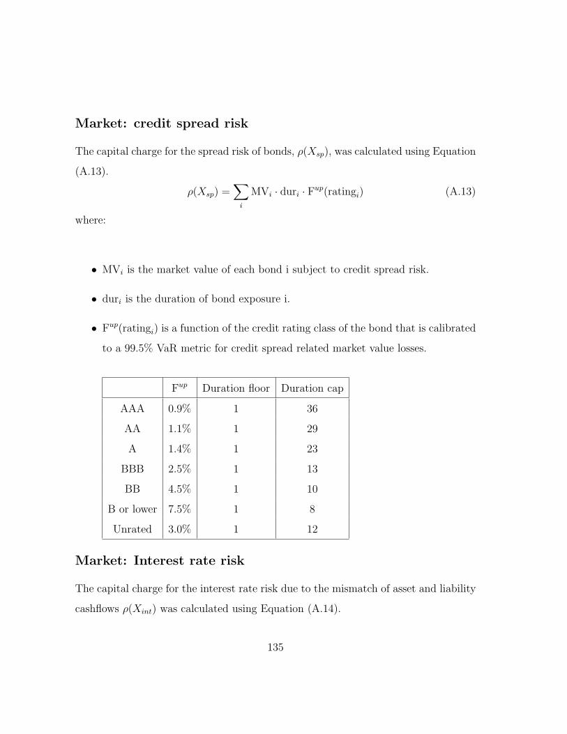
Market: credit spread risk
The capital charge for the spread risk of bonds, ρ(Xsp), was calculated using Equation
(A.13).
ρ(Xsp) =∑i
MVi · duri · Fup(ratingi) (A.13)
where:
• MVi is the market value of each bond i subject to credit spread risk.
• duri is the duration of bond exposure i.
• Fup(ratingi) is a function of the credit rating class of the bond that is calibrated
to a 99.5% VaR metric for credit spread related market value losses.
Fup Duration floor Duration cap
AAA 0.9% 1 36
AA 1.1% 1 29
A 1.4% 1 23
BBB 2.5% 1 13
BB 4.5% 1 10
B or lower 7.5% 1 8
Unrated 3.0% 1 12
Market: Interest rate risk
The capital charge for the interest rate risk due to the mismatch of asset and liability
cashflows ρ(Xint) was calculated using Equation (A.14).
135
ρ(Xint) = max(Mktupint,Mktdownint ) (A.14)
where:
Mktupint = NAV |upshock is the change in the Net Asset Value due to a pre-
scribed upward shock to interest rates. Mktdownint = NAV |down is the change in net
assets due to a prescribed downward shock to interest rates. The interest rate shocks
are calibrated to VaR 99.5% over a one-year period.
Operational risk
The current-year capital charge for operational risk, ρ(Xop), was based on Equation
(A.15).
ρ(Xop) = min(0.3× BSCR;max(0.03× EP; 0.003× TP)) (A.15)
where:
• BSCR is the Basic Solvency Capital Requirement i.e. the sum of all the risk
charges calculated above including diversification credits, and before adjust-
ments for the risk reduction arising from future profit sharing and deferred
taxes (which we have ignored).
• EP is the total earned premium (gross of reinsurance, if any) for the term life
portfolio in the year following the valuation date
136

• TP are the Technical Provisions on the valuation date. Best estimate provisions
are required to be used in the computation to avoid circularity (since the cost
of capital margin in TP includes a charge for operational risk).
137
Appendix B
Assumptions for Chapter 4
calculations
B.1 Mortality table assumption
The mortality rates that were used to perform the calculations in Chapter 4 are given
in Table B.1 of this appendix.
B.2 Initial interest rates
The interest rates on the starting date of the monte-carlo simulation experiments of
Chapter 4 are given in Table B.2 of this appendix.
138

Age q(x) Age q(x) Age q(x)
31 0.00109 56 0.00491 81 0.07543
32 0.00114 57 0.00542 82 0.08332
33 0.00118 58 0.006 83 0.09187
34 0.00119 59 0.00666 84 0.10112
35 0.00118 60 0.0074 85 0.11113
36 0.00116 61 0.00824 86 0.12191
37 0.00115 62 0.00919 87 0.13354
38 0.00115 63 0.01026 88 0.14605
39 0.00118 64 0.01147 89 0.15949
40 0.00122 65 0.01284 90 0.17393
41 0.00131 66 0.01439 91 0.18941
42 0.0014 67 0.01614 92 0.20598
43 0.00152 68 0.0181 93 0.22371
44 0.00164 69 0.02031 94 0.24263
45 0.00178 70 0.02279 95 0.26281
46 0.00194 71 0.02555 96 0.28427
47 0.00212 72 0.02864 97 0.30704
48 0.00231 73 0.03207 98 0.33115
49 0.00253 74 0.03587 99 0.35658
50 0.00277 75 0.04007 100 0.38543
51 0.00304 76 0.04471 101 0.42814
52 0.00334 77 0.0498 102 0.49724
53 0.00367 78 0.05539 103 0.60527
54 0.00403 79 0.0615 104 0.76478
55 0.00445 80 0.06817 105 1
Table B.1: 1986-92 Canadian CIA basic male, ultimate, non-smoker, nearest age
139
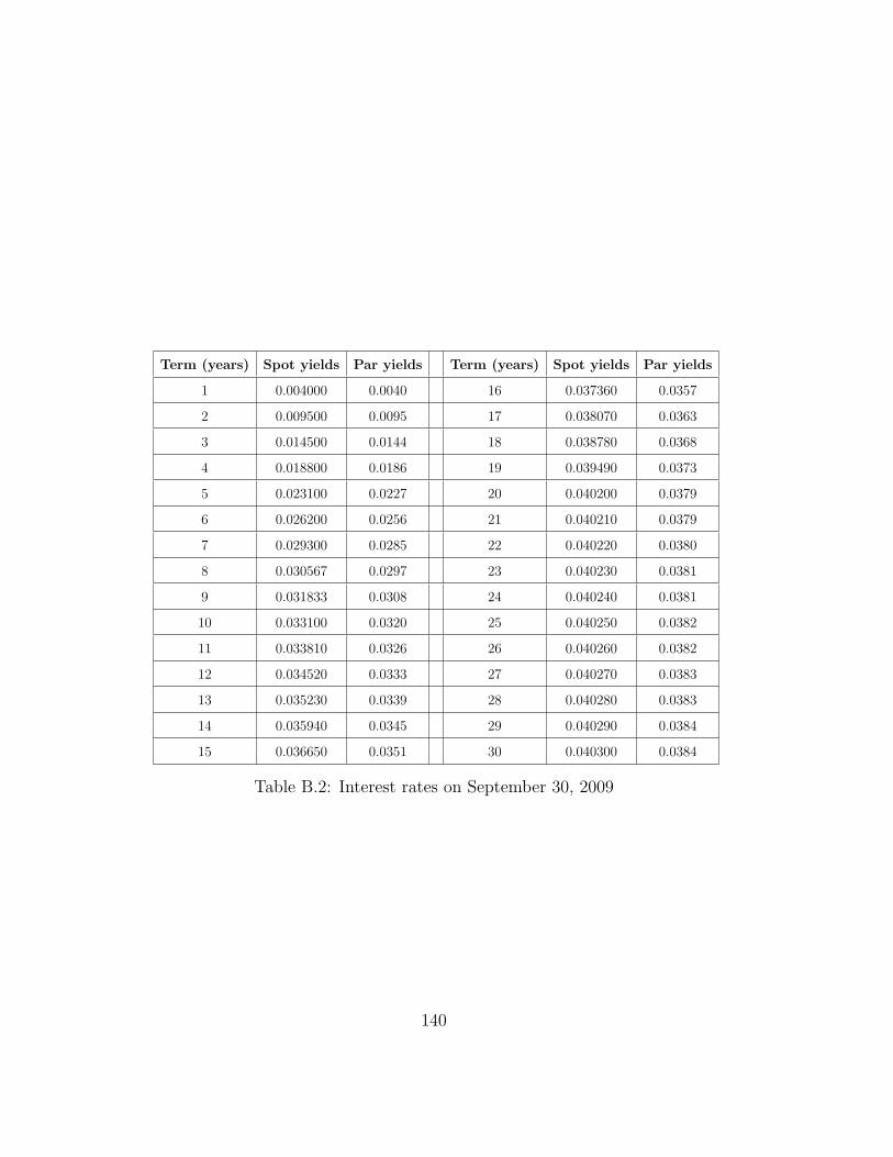
Term (years) Spot yields Par yields Term (years) Spot yields Par yields
1 0.004000 0.0040 16 0.037360 0.0357
2 0.009500 0.0095 17 0.038070 0.0363
3 0.014500 0.0144 18 0.038780 0.0368
4 0.018800 0.0186 19 0.039490 0.0373
5 0.023100 0.0227 20 0.040200 0.0379
6 0.026200 0.0256 21 0.040210 0.0379
7 0.029300 0.0285 22 0.040220 0.0380
8 0.030567 0.0297 23 0.040230 0.0381
9 0.031833 0.0308 24 0.040240 0.0381
10 0.033100 0.0320 25 0.040250 0.0382
11 0.033810 0.0326 26 0.040260 0.0382
12 0.034520 0.0333 27 0.040270 0.0383
13 0.035230 0.0339 28 0.040280 0.0383
14 0.035940 0.0345 29 0.040290 0.0384
15 0.036650 0.0351 30 0.040300 0.0384
Table B.2: Interest rates on September 30, 2009
140
B.3 The C-3 phase III interest rate generator: model
specification
The following is a description of the Stochastic Log Volatility (SLV) Model. The SLV
model simulates the following three (3) correlated stochastic processes in discrete
monthly time:
1. 1it: The natural logarithm of the long maturity interest rate
2. αt: The nominal spread between the long and short maturity rates
3. υt: The natural logarithm of the volatility of the long maturity rate process
The SLV discrete time equations are:
1it = max⟨1λL,min1λU , (1−β1) ·1 it−1+β1 · log τ1+ψ(2τt−αt−1)⟩+1 σt ·1Zt (B.1)
αt = (1− β2) · αt−1 + β2 ·2 τt + ϕ(1it−1 − log τ1) +1 σ2 ·2 Zt · (1rt−1)θ (B.2)
υt = (1− β3) · υt−1 + β3 · log τ3 + σ3 ·3 Zt (B.3)
where
1it=log 1rt
1λU=log 1rmax
1λL=log 1rmin
2rt=exp 1it − αt
If 2rt <2 rmin, then 2rt = κ ·1 rt · αt
1σt = exp (υt)
1Zt,2 Zt and 3Zt ∼ N(0, 1) with constant correlation matrix ρ
141

B.4 Simulated sample key interest rates from the
C3 Phase III generator
The sample distributions of the 1, 7, 10 and 30 year spot interest rates based on the
10,000 C3 Phase III generator scenarios that were used in the analysis of Chapter 4
are summarized in Figure B.1 of this appendix.
142
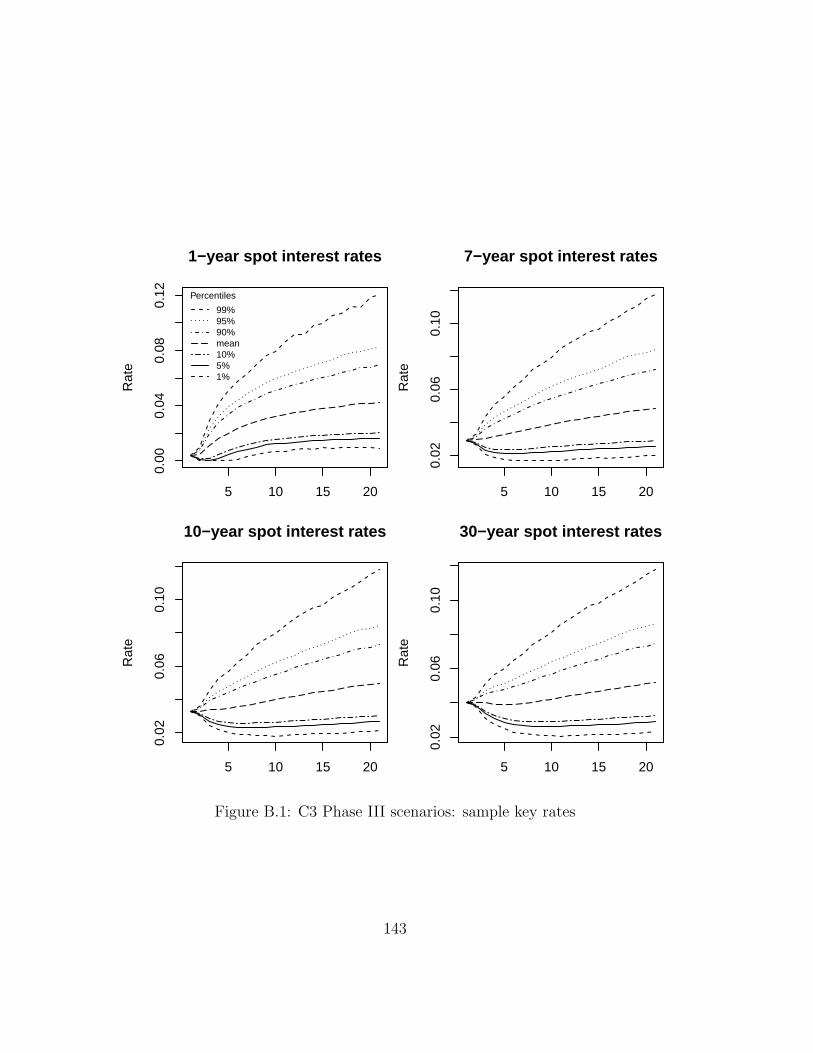
Rat
e
5 10 15 20
0.00
0.04
0.08
0.12
1−year spot interest rates
Percentiles
99%95%90%mean10%5%1%
Rat
e
5 10 15 20
0.02
0.06
0.10
7−year spot interest rates
Rat
e
5 10 15 20
0.02
0.06
0.10
10−year spot interest rates
Rat
e
5 10 15 20
0.02
0.06
0.10
30−year spot interest rates
Figure B.1: C3 Phase III scenarios: sample key rates
143
Bibliography
AAA (2002). Principle-Based Risk-Based Capital Report. American Academy of
Actuaries (AAA).
AAA (2003). Recommended Approach for Setting Regulatory Risk-Based Capital
for Variable Products with Guarantees (Excluding Index Guarantees). American
Academy of Actuaries (AAA).
AAA (2008a). C3 Life and Annuity Capital Work Group’s Presentation to the
National Association of Insurance Commissioners Life Risk Based Capital Work
Group. American Academy of Actuaries (AAA).
AAA (2008b). Report from the American Academy of Actuaries’ Economic Scenario
Work Group. American Academy of Actuaries (AAA).
Artzner, P., Delbaen, F., Eber, J.-M., and Heath, D. (1999). Coherent Measures of
Risk. Mathematical Finance, 9(3):203–228.
ASB (Canada) (2009). Standards of Practice - Practice-Specific Standards for Insur-
ers. Actuarial Standards Board (Canada).
Babbel, D., Gold, J., and Merrill, C. L. (2002). Fair Value of Liabilities: The Financial
Economics Perspective. North American Actuarial Journal, 6(1):12–27.
144
Bader, L. N. and Gold, J. (2003). Reinventing Pension Actuarial Practice. Pension
Forum, 14(2):1–13.
BIS (1988). International Convergence of Capital Measurement and Capital Stan-
dards. Basel Committee on Banking Supervision, Bank for International Settle-
ments (BIS).
BIS (1996). Amendment to the Basel Capital Accord to Incorporate Market Risk.
Basel Committee on Banking Supervision, Bank for International Settlements
(BIS).
BIS (2006). Basel II: International Convergence of Capital Measurement and Capital
Standards: A Revised Framework - Comprehensive Version. Basel Committee on
Banking Supervision, Bank for International Settlements (BIS).
BIS (2010). Basel III: A global regulatory framework for more resilient banks and
banking systems. Basel Committee on Banking Supervision, Bank for International
Settlements (BIS).
Black, F. and Scholes, M. (1973). The pricing of options and corporate liabilities.
Journal of political economy.
Boyle, P. P. and Hardy, M. R. (1997). Reserving for Maturity Guarantees: Two
Approaches. Insurance: Mathematics and Economics, 21(2):113–127.
Boyle, P. P. and Hardy, M. R. (2007). Financial Engineering: Applications in Insur-
ance. In Handbook of Financial Engineering. Wiley (New York).
CEIOPS (2010). QIS5 Technical Specifications. Committee of European Insurance
and Occupational Pension Supervisors.
145

Cummins, J., Harrington, S., and Klein, R. (1995). Solvency experience, risk-based
capital, and prompt corrective action in property-liability insurance. Journal of
Banking and Finance.
Cummins, J., Harrington, S., and Niehaus, G. (1993). An economic overview of risk-
based capital requirements for the property-liability insurance industry. Journal of
Insurance Regulation, 11:427–447.
Doff, R. (2008). A critical analysis of the Solvency II proposals. The Geneva Papers
on Risk and Insurance - Issues and Practice, 33:193–206.
Eling, M. (2010). What do we know about market discipline in insurance?. University
of Ulm, Germany.
Eling, M., Schmeiser, H., and Schmit, J. T. (2007). The Solvency II Process: Overview
and Critical Analysis. Risk Management and Insurance Review, 10(1):69–85.
Embrechts, P., Lindskog, F., and McNeil, A. (2001). Modelling Dependence with Cop-
ulas and Applications to Risk Management. Department of Mathematics, ETHZ.
Hardy, M. R. (1993). Stochastic Simulation in Life Office Solvency Assessment. Jour-
nal of the Institute of Actuaries, 120:II:131–152.
Hardy, M. R. (2003). Investment Guarantees: Modelling and Risk Management for
Equity-Linked Life Insurance. Wiley, New York.
Hirst, D., Koonce, L., and Venkataraman, S. (2007). How disaggregation enhances
the credibility of management earnings forecasts. Journal of accounting research.
Hull, J. and White, A. (1993). One-factor interest-rate models and the valuation of
interest-rate derivative securities. Journal of financial and quantitative analysis.
146

IAA (2004). A Global Framework for Insurer Solvency Assessment. International
Actuarial Association (IAA).
IAIS (2002). Principles on Capital Adequacy and Solvency, Principles No. 5. Inter-
national Association of Insurance Supervisors (IAIS).
IAIS (2005). Towards a Common Structure and Common Standards for the As-
sessment of Insurance Solvency: Cornerstones for the Formulation of Regulatory
Financial Requirements. International Association of Insurance Supervisors (IAIS).
IAIS (2007). IAIS Common Structure for the Assessment of Insurance Solvency.
International Association of Insurance Supervisors (IAIS).
IASB (2010). Exposure Draft Insurance Contracts.
IASB(2007). International Accounting Standards Board’s Discussion Paper: Prelim-
inary Views on Insurance Contracts.
JCOAA (2008a). Framework for a New Standard Approach to Setting Capital Re-
quirements. Joint Committee of OSFI, AMF, and Assuris (JCOAA).
JCOAA (2008b). Standardized Approach for Calculating the Solvency Buffer for
Market Risk. Joint Committee of OSFI, AMF, and Assuris (JCOAA).
Jorion, P. (2005). Financial Risk Manager Handbook Third Edition. John Wiley &
Sons, Inc.
Kim, D. and Santomero, A. (1988). Risk in banking and capital regulation. Journal
of Finance.
147
Klugman, S., Panjer, H., and Willmot, G. (1998). Loss Models. John Wiley, New
York.
Linder, U. and Ronkainen, V. (2004). Solvency II Towards a new insurance supervi-
sory system in the EU. Scandinavian Actuarial Journal, (6):462–474.
Lombardi, L. J. (2006). Valuation of Life Insurance Liabilities. ACTEX Publications,
Inc.
MAC (2007). Canadian Vision for Life Insurer Solvency Assessment. Minimum Con-
tinuing Capital and Surplus Requirements Advisory Committee (MAC).
McNeil, A., Frey, R., and Embrechts, P. (2005). Quantitative Risk Management.
Princeton University Press, New Jersey.
Merton, R. C. (1974). On the pricing of corporate debt: The risk structure of interest
rates. Journal of Finance.
Modigliani, F. and Miller, M. H. (1958). The cost of capital, corporation finance and
the theory of investment. The American Economic Review.
NAIC (2008). Life Risk-Based Capital Report. National Association of Insurance
Commissioners (NAIC).
OSFI (2008). Minimum Continuing Capital and Surplus Requirements (MCCSR) for
Life Insurance Companies.
OSFI (2010a). Guidance for the Development of a Model-Based Solvency Framework
for Canadian Life Insurance Companies.
148
OSFI (2010b). Minimum Continuing Capital and Surplus Requirements (MCCSR)
for Life Insurance Companies.
Panjer, H. H. (2001). Measurement of risk, solvency requirements and allocation of
capital within financial conglomerates. IIPR technical report 01-14, University of
Waterloo.
Panjer, H. H., Boyle, P. P., Cox, S. H., Dufresne, D., Gerber, H. U., Mueller, H. H.,
Pedersen, H. W., Pliska, S. R., Sherris, M., Shiu, E. S., and Tan, K. S. (1998).
Financial economics: With applications to investments, insurance and pensions.
The Actuarial Foundation.
Plantine, G. and Rochet, J.-C. (2007). When Insurers Go Bust. An Economic Anal-
ysis of the Role and Design of Prudential Regulation. Princeton University Press.
Porter, M. (1980). Competitive Strategy. Free Press, New York.
Reddington, F. (1952). Review of the principle of life-office valuations. Journal of
the Institute of Actuaries.
Rochet, J. (1992). Capital requirements and the behaviour of commercial banks.
European Economic Review.
Sandstrom, A. (2006). Solvency: Models, Assessment and Regulation. Chapman &
Hall/CRC.
Sharma, P. (2002). Prudential Supervision of Insurance Undertakings.
Towers Perrin (2004). How Might the Presentation of Liabilities at Fair Value Have
Affected the Reported Results of U.S. Property and Casualty Insurers?
149
Vaughan, T. M. (2009). The Implications of Solvency II for U.S. Insurance Regulation.
Networks Financial Institute Policy Brief No. 2009-PB-03.
Wallace, M. (2006). The problem with current accounting: A critique of SFAS 115
and SFAS 133 using an equity-indexed annuity example. North American Actuarial
Journal.
Wirch, J. L. and Hardy, M. R. (1999). A synthesis of risk measures for capital
adequacy. Insurance: Mathematics and Economics, 25(3):337–347.
150