1

Toward a Dynamic Notion of Value Creation and Appropriation in Firms:

The Concept and Measurement of Economic Gain

Marvin B. Lieberman Natarajan Balasubramanian UCLA Anderson School of Management

110 Westwood Plaza, B415 Los Angeles, CA 90095-1481

Tel.: (310) 206-7765 marvin.lieberman@anderson.ucla.edu

Whitman School of Management 721 University Ave. Syracuse, NY 13244 Tel.: (315) 443-3571 nabalasu@syr.edu

Roberto Garcia-Castro IESE Business School

Camino del Cerro del Águila, 3 28023 Madrid-Spain

Tel.: (34) 91 211 30 00 rgarcia@iese.edu

September 1, 2016

Research Summary: ‘Value creation’ is central to strategy. Even so, confusion arises because it can be defined in different ways, e.g., as the sum of producer and consumer surplus in a given time period, or as the change in surplus over time. To formalize the latter notion we introduce the concept of economic gain, defined as the increase in total surplus. Economic gain can arise through innovation or when a superior firm displaces competitors. We provide a firm-level measurement framework to quantify economic gain and its distribution among stakeholders, including the firm’s shareholders, employees, suppliers, and customers. As an empirical illustration, we compare the creation and distribution of economic gain by Southwest Airlines and American Airlines between 1980 and 2010.

Managerial Summary: Most managers and the business press regard ‘value creation’ as the increase in shareholder wealth represented by a rise in corporate profit or stock price. A broader conception of value creation goes beyond shareholders to include the value that is distributed to additional stakeholders of the firm, including employees, suppliers, and customers. We develop a mathematical framework that allows this broader notion of value creation and distribution to be assessed and quantified in many cases. We illustrate the framework using historical data on Southwest Airlines and American Airlines over three decades.

Keywords: value creation, value distribution, value appropriation, stakeholders, economic gain

2

INTRODUCTION

The notion that firms create and distribute economic value is central to the field of strategic

management. Several streams of research—in particular, the resource-based view of the firm (RBV),

the stakeholder theory of the firm, and more recently, value-based strategy (VBS)—explicitly focus

on questions of value creation and capture.1 Despite this centrality of ‘value creation’ within the

field, there has been a lack of clarity on the precise meaning of the concept. Without clear

definitions and suitable empirical tools, researchers have rarely attempted to measure the total

economic value created by a firm or its distribution among key stakeholders.

A major source of confusion is that value creation can be reasonably defined in two different

ways: first, as the total economic value created by a firm within a specific interval of time (sum of

consumer and producer surplus); and second, as the change in this value over longer periods. We

call the first definition ‘static value creation’, and the second, ‘dynamic value creation’ or ‘economic

gain’. While both are useful concepts, the dynamic notion has been largely ignored in strategic

management and is comparatively undeveloped. This is surprising given that the common view of

value creation by a CEO is explicitly dynamic: shareholders want the CEO to increase the firm’s

profit and stock price over time.

Drawing together concepts from economics and strategic management, we show that

economic gain has two components, which we call ‘innovation’ and ‘replication’. A firm may

improve through cost reductions or through quality improvements that increase customers’

willingness to pay (WTP). We refer to these broadly as ‘innovation’, recognizing that they may arise 1In the RBV (e.g., Wernerfelt, 1984; Barney, 1991) the economic value created by a firm arises from the scarcity of valuable resources and competitors’ difficulty in imitating or substituting them. The stakeholder theory views the firm as ‘a constellation of cooperative and competitive interests possessing intrinsic value’ (Donaldson and Preston, 1995, p. 66) and focuses on value capture by these stakeholders. Similarly, VBS uses game theory to model coalitions of agents who cooperate to create value and then compete to capture it (Brandenburger and Stuart, 1996; MacDonald and Ryall, 2004; Makadok, 2011; Chatain and Zemsky, 2011).

3

from various sources internal and external to the firm. In addition, a firm that is superior to its

rivals can create value by expanding at the expense of competitors, thereby serving more customers

who may benefit from the firm’s higher quality or lower cost. We refer to this second type of value

creation as ‘replication’.2 While the two components are related—replication creates value only if the

firm has previously been innovative relative to rivals—it is useful to distinguish them in assessing the

process of value creation. Given our focus on specific firms, we ignore value creation that may come

from exogenous growth in industry demand.

We adapt methods from the literature on productivity measurement to estimate these

components of dynamic value creation, as well as the distribution of value among the firm’s

stakeholders. In some contexts it is possible to derive the estimates from standard corporate

accounting data. Although we cannot directly overcome the problem of measuring consumer

surplus, which hinders most empirical efforts to estimate the total economic value created by a firm,

we show that under some assumptions this problem can be reasonably addressed in a dynamic

context. To make our concepts and measures more concrete, we provide an illustration of dynamic

value creation for Southwest Airlines (SWA) and American Airlines (AA) over the interval from

1980 to 2010.

Our theoretical exposition of economic gain and the associated measurement framework

make several contributions to the strategic management literature. (A related empirical study,

Lieberman, Garcia-Castro and Balasubramanian (2016), analyzes a larger sample of airline and

automotive companies, thereby providing more comprehensive evidence on inter-firm and inter-

stakeholder variation as well as guidance on data implementation.) At the broadest level we clarify

that value creation by a firm can be viewed and potentially quantified in the alternative ways that we

2 Although quantity changes are not alien to VBS (e.g., Bennett, 2013; Stuart, 2007) they have not been extensively studied. Our discussion brings to the surface the fact that innovation gains and quantity changes are both fundamental in how firms create and capture value.

4

call ‘static’ and ‘dynamic’. The ‘static’ notion (total surplus) is widely recognized, but the dynamic

notion (change in surplus) is often more relevant and measurable.

The ability to estimate economic gain and its distribution among the firm’s stakeholders has

the potential to facilitate conversations among theoretical strands of the strategic management

literature—especially the RBV, the stakeholder view, and the VBS. Furthermore, economic gain

links with the concept of competitive advantage, which is often defined as a firm’s ability to create

greater economic value than competitors. Achieving economic gain is a necessary condition to

increasing competitive advantage. Like economic gain, competitive advantage is now regarded as

relating to all stakeholders (Peteraf and Barney, 2003; Coff, 1999, 2010), whereas most studies of

firm performance have been limited to measuring shareholder value. Thus, compared with prior

empirical work in strategic management, our measurement framework offers a more comprehensive

assessment of a firm’s value creation and distribution.

ALTERNATIVE CONCEPTS AND MEASURES OF VALUE CREATION

Confusion about value creation arises from at least two sources. As described above, one source of

confusion relates to whether the concept is ‘static’ or ‘dynamic.’ A second source relates to the

corporate stakeholders under consideration: only shareholders, or a more inclusive set. Table 1

classifies common concepts and measures of corporate value creation along these dimensions.

--Insert Table 1 about here--

Shareholder value versus total value creation

The most commonly considered stakeholders are the firm’s shareholders. Shareholder value creation

and associated measures (profits, market capitalization, etc.) are standard concepts. Using simple

ratios such as return on assets or equity, the firm’s profit rate can easily be compared over time or

relative to competitors. More sophisticated measures such as ‘economic value added’ subtract out

the firm’s cost of capital in order to estimate true economic profit. Countless studies draw upon

5

such measures, which can be readily computed from available data.

Such a focus on shareholder value has two main limitations. First, by considering only a

single, albeit important, stakeholder, it offers a limited perspective, ignoring most of the economic

value typically created and distributed by a firm. Second, it provides only a partial insight into how

firms create value: managers can create value for shareholders by enlarging the total value created by

the firm or simply by redistributing rents. Actions that expand the total pie are fundamentally

different from those that merely carve a larger slice for shareholders, with distinct implications for

stakeholders and society.

Going beyond shareholders, the concept of total economic value is usually defined as the gap

between the customer’s WTP and the supplier’s opportunity cost. This approach can be formulated

within the context of supply and demand curves (e.g., Besanko, Dranove, Shanley, and Schaefer,

2012) or in a bargaining framework (e.g., Brandenburger and Stuart, 1996). Although broader than

shareholder value, this concept of economic value (total surplus) usually limits its attention to two

stakeholders: shareholders and consumers.3

Empirical applications of the concept of total value creation are constrained by difficulties in

measuring WTP and opportunity costs. To overcome these challenges, a growing number of studies

in industrial organization economics develop models of competition that incorporate structural

estimates of costs and demand, thereby providing assessments of producer and consumer surplus.

(See Ackerberg et al., 2007, for a review of this literature.) These studies typically examine a single

industry, modeling specific features of the industry context to obtain moment conditions that allow

supply and demand to be identified.4

While the structural estimation approach has been used primarily to answer policy questions 3 Brandenburger and Stuart (1996) include three stakeholders: suppliers, the firm, and customers. 4 A recent example in the strategy literature is Grennan (2014), which develops such a model to measure the importance of bargaining ability in determining the division of value between coronary stent producers and their customers (hospitals).

6

in economics, it offers promise for addressing questions in strategic management. A major strength

of the structural approach is the ability to incorporate idiosyncratic firm or industry data to identify

determinants of the economic surplus and its division among parties. Although studies in this vein

have focused almost exclusively on characterizing effects at the industry level, the approach can be

applied to questions at the level of individual firms.

Static versus dynamic value creation

Within the two notions of value creation described above—shareholder value and total economic

value—a second dimension relates to timeframe. Measures such as accounting profits, economic

value added (EVA), residual income, and the economic value created (e.g., Brandenburger and

Stuart, 1996; Davis and Kay, 1990) are static in that they focus on value created in a single time

period. In contrast, the business press and much of the scholarly literature describe (shareholder)

value creation as dynamic: an increase in the firm’s stock market value. The common notion of a

value-creating CEO is not one who presides over a firm with large profits or stock market

capitalization, but rather a CEO who is able to raise the firm’s profit and stock price over time.

Shareholders want the CEO not simply to maintain the firm but to grow it in a profitable way; it is

rare that a CEO is judged based on the level of shareholder wealth and not on the changes.5

Furthermore, a dynamic framework emphasizes the need to consider stakeholders beyond

shareholders in order to fully understand the flow of economic value. Firms that create new value

may distribute it in different ways depending upon competition, legal rights, bargaining power, and

so on. For example, a firm that introduces an innovation with strong patent protection is likely to be

in a position to appropriate much of the innovation’s value for its shareholders or employees. By

comparison, in an environment where technology is improving but difficult to protect from

imitation, most if not all of the new economic value will flow downstream to consumers. The 5 Moreover, arguments from behavioral economics suggest that human utility adjusts to a reference point and is thus more sensitive to changes than to absolute levels (Kahneman, 2011).

7

computer industry is perhaps the best example: prices of computers and profits of computer

manufacturers have fallen over the past three decades even though innovations have exponentially

improved the quality of computers used by customers.

To summarize, the conceptualization of value creation differs greatly across the quadrants in

Table 1. Concepts of shareholder value creation—both static and dynamic—are well established, and

good empirical measures are in wide use. With regard to total value creation, static concepts are well

developed, but the difficulty of measuring consumer surplus limits their empirical application.

Dynamic concepts and measures of total value creation have gone almost completely unrecognized

in strategic management, and tools for assessing value capture by multiple stakeholders remain

rudimentary and ad hoc. This suggests the need for concepts and methods to characterize growth in

total economic value and the distribution of that value among stakeholders of the firm. The

remainder of this paper develops such a concept: ‘economic gain’.6

ECONOMIC GAIN: A DYNAMIC NOTION OF TOTAL VALUE CREATION

Concept

We define economic gain as the change in economic value (total surplus) created by a firm from one

period to the next. We begin by illustrating the notion of economic gain arising from an innovation.

Consider Firm A facing a single competitor Firm B in some industry. Suppose in period 0, the two

firms are identical, and the economic value created by each is ν0Y0, where ν is the average economic

value created per unit (i.e., the average difference between WTP and cost), Y is the number of units

of output, and the subscript refers to the period. Now, suppose Firm A develops a single innovation

in period 1, and that innovation has two types of effects that last over two periods. First, the

innovation increases the average value created in each period by Δν1 to ν1. Second, this innovation

allows the firm to grow by taking away some of its competitors’ customers. In particular, suppose

6 We thank Arnold Harberger for suggesting this term.

8

Firm A grows to Y1=Y0+ΔY1 in period 1 and to Y2=Y1+ΔY2 in period 2.7 For simplicity, we make

the following assumptions: (a) Firm A grows by taking customers away from Firm B8; (b) Firm A

does not innovate in period 2; (c) Firm B does not innovate in periods 1 and 2.9 Then, the economic

value created by Firm A in period 1 is given by:

ν1Y1= (ν0 + Δν1)( Y0+ΔY1) (1)

However, some of this value is created by Firm A simply replacing Firm B. In particular, if Firm B

had not contracted, then it would have created ν0ΔY1 of economic value that is now by created by

Firm A (by assumption, the average value created by Firm B does not change and stays at ν0).

Excluding this inter-firm transfer and subtracting the economic value created by Firm A in period 0

from Equation (1) gives the economic gain for Firm A in period 1:

Γ1 = Y0Δν1 + Δν1ΔY1 (2)

Turning to period 2, Firm A’s economic value created equals:

ν1Y2= (ν0 + Δν1)( Y0+ΔY1+ΔY2) (3)

Note that we use ν1 as the average value created, since by assumption, Firm A does not innovate in

period 2. As before, a part of this economic value created (ν0ΔY2) is purely an inter-firm transfer

from Firm B to Firm A. Excluding this inter-firm transfer and subtracting the economic value

created by Firm A in period 1 from Equation (3), gives the economic gain for Firm A in period 2:

Γ2 = (ν1 – ν0)ΔY2 (4)

Thus, the total economic gain for Firm A from its innovation in period 1 is given by:10 7 If there were no costs to expanding the firm, the firm could expand and occupy the whole industry instantly. However, that is unlikely, and hence, a firm will spread out its growth over multiple periods. 8 More broadly, firm A may grow at the expense of several firms, including firms outside the industry. This discussion can be generalized to those situations. 9 In general, firm B may also innovate and increase its average value created over time. We discuss this later in the text as well as in Online Appendix B and C. 10 We use (ν1 – ν0) in the last term of Equation (5) rather than Δν1 to make it more apparent that the comparison for replication gain is with an outside firm or industry average (see Equation (6)).

9

Γ = Γ1 + Γ2 = {Y0Δν1 + Δν1ΔY1} + (ν1 – ν0)ΔY2 (5) ‘innovation gain in Period 1’ ‘replication gain in Period 2’

Hence, a firm can achieve economic gain in two broad ways. First, and corresponding to the

first two terms of Equation (5), value is created through innovations within firms that increase the

average economic value created per unit over its current output (Y0Δν1) and allow the firm to

expand by immediately displacing some competitors (Δν1ΔY1). We term this as ‘innovation gain’.

Broadly, innovations increase the customer’s WTP for the product (without proportionately

increasing the opportunity costs), or decrease the opportunity costs (without proportionately

decreasing the customer’s WTP).11 The second way of achieving economic gain, ‘replication gain’,

corresponding to the third term of Equation (5), is when the superior firm, based on its past

innovations, grows relative to its competitors.12

--Insert Figure 1 about here--

We illustrate this graphically in Figure 1 for a cost-reducing innovation.13 In Period 0, Firm A

is identical to its competitors, with a unit cost of C0 and an output, Y0. The price is p0=C0. All the

economic value created, equal to the area between the demand and supply curves, is appropriated by

the customers. The firm and its stakeholders receive their opportunity costs.

In Period 1, Firm A innovates and reduces its unit costs to C1. Thus, the firm has created

additional value (Δν1 = ν1 – ν0 = C0 - C1) by freeing up resources that can be used elsewhere. Now,

11 We include in the category of gains from innovation a range of enhancements that are under the firm’s control, such as unit cost reductions from economies of scale. Note that WTP and opportunity costs may also change due to factors outside the control of the firm. However, given our focus on economic value that arises through the actions of a firm, we exclude these possibilities from the concept of economic gain. 12 The covariance term (Δν1ΔY1) could potentially be assigned to replication gain. However, this requires an unrealistic assumption of no firm growth in period 1 and is inconsistent with our measurement framework for innovation gain. (See below and proofs of Propositions 1 and 2 in the Online Appendix.) 13 Online Appendix A provides additional graphical illustrations including on the static notions of value creation. That appendix also lays out the assumptions underlying these graphical illustrations.

10

Firm A expands output to Y1 in this period by taking customers away from its competitors. Firm A’s

economic gain in period 1 is the sum of the two hatched rectangles (corresponding to the two terms

in Equation (2) or the two terms corresponding to ‘innovation gain in Equation (5)). The hatched

rectangle to the left of Y0 corresponds to the gain from having a lower cost in existing

markets/customers (Y0Δν1). The hatched rectangle between Y0 and Y1 is the gain from immediately

displacing some of its less-efficient competitors, and expanding output (Δν1ΔY1).

In the next period, Period 2, Firm A does not innovate further, but leverages its innovation

from period 1 and expands output to Y2 by further displacing its competitors. Then, Firm A’s

economic gain in Period 2 is solely due to replication of its competitive advantage in Period 1. This

corresponds to Equation (4) (or the last term in Equation (5)), (ν1 – ν0)ΔY2, and is equal to the area

of the dotted rectangle between Y1 and Y2 in Figure 1.14 There are several real-life examples of such

economic gain. Many successful firms such as McDonald’s, Starbucks, and Walmart started with an

innovation that provided them an initial advantage over their competitors, and then expanded over

time by leveraging that innovation. Later in this article, we discuss the example of Southwest

Airlines, and show that it appears to have followed a similar path. Such replication is a common type

of strategy, particularly when productive units are specific to a geographic area (Winter and

Szulanski, 2001, Bowman and Ambrosini, 2003; Jonsson and Foss, 2011).

While the above illustration focuses on a cost reduction, economic gain from innovations

that increase WTP is conceptually similar. Firms that are able to increase their customers’ WTP, say

by improving product quality, will increase the per-unit value created, and eventually grow by

14 Note that the same total economic gain would be achieved if Firm B had immediately copied and fully implemented Firm A’s innovation, thereby preventing Firm A’s displacement of Firm B. In the next section, we will include such imitation as a form of innovation gain. The concept of replication gain is needed in our framework to capture economic gains associated with changes in market share. (If market shares remain stable in an industry with constant demand, all economic gain will be innovation gain.)

11

displacing their competitors. Thus, to summarize, economic gain arises when a firm reduces its cost

or increases the customers’ WTP through innovation, or when a superior firm grows at the expense

of its competitors.

Now, we briefly discuss two sources of value creation ignored here. The preceding

discussion assumes that the focal firm’s competitors do not innovate, and that industry output stays

constant (at YIND(0,1,2)) in Figure 1. However, firms may imitate innovations from their competitors or

adopt innovations from outside the industry. Then, the per-unit value created by competitors will

also increase over time, and in the extreme case, competitors are eventually able to match the focal

firm’s cost (or WTP). This causes industry output to increase (to YIND(N) in Figure 1). Further, this

brings new ‘extra-marginal’ customers into the industry, as firms lower their prices (or improve their

products). The economic value created for these additional customers is depicted in Figure 1 as the

solid triangle towards the right of the figure. This is the familiar ‘Harberger triangle’ (Harberger,

1954, 1964; Hines, 1998), which is often small compared to the gains from innovation. We briefly

discuss this aspect later in the paper.

We also ignore an additional way in which economic value may be created within an

industry: exogenous growth in demand. Changes in consumer tastes, growth in population or

income, or increases in the prices of substitute products may shift the industry demand curve in a

manner that increases the consumer surplus generated by the industry. We exclude this type of value

creation from the concept of economic gain, as it is independent of the actions of firms in the

industry. Accordingly, our definition of economic gain through replication refers to expansion of a

superior firm that increases its market share. Given this focus, we also exclude any value creation

that may arise when a firm diversifies into a new industry.

Turning to measurement, the notion of economic gain has a major advantage: at least a part of

it can be reasonably and generally estimated using publicly available data on inputs, outputs, costs,

12

and prices (including potential adjustments for quality). Because it considers only period-to-period

changes, under some assumptions, it circumvents the problem of estimating WTP and opportunity

costs. This allows us to estimate innovation gains in many situations, and replication gains in some

situations. Such a general approach to measuring a firm’s economic gain from innovation is

discussed in the next section.

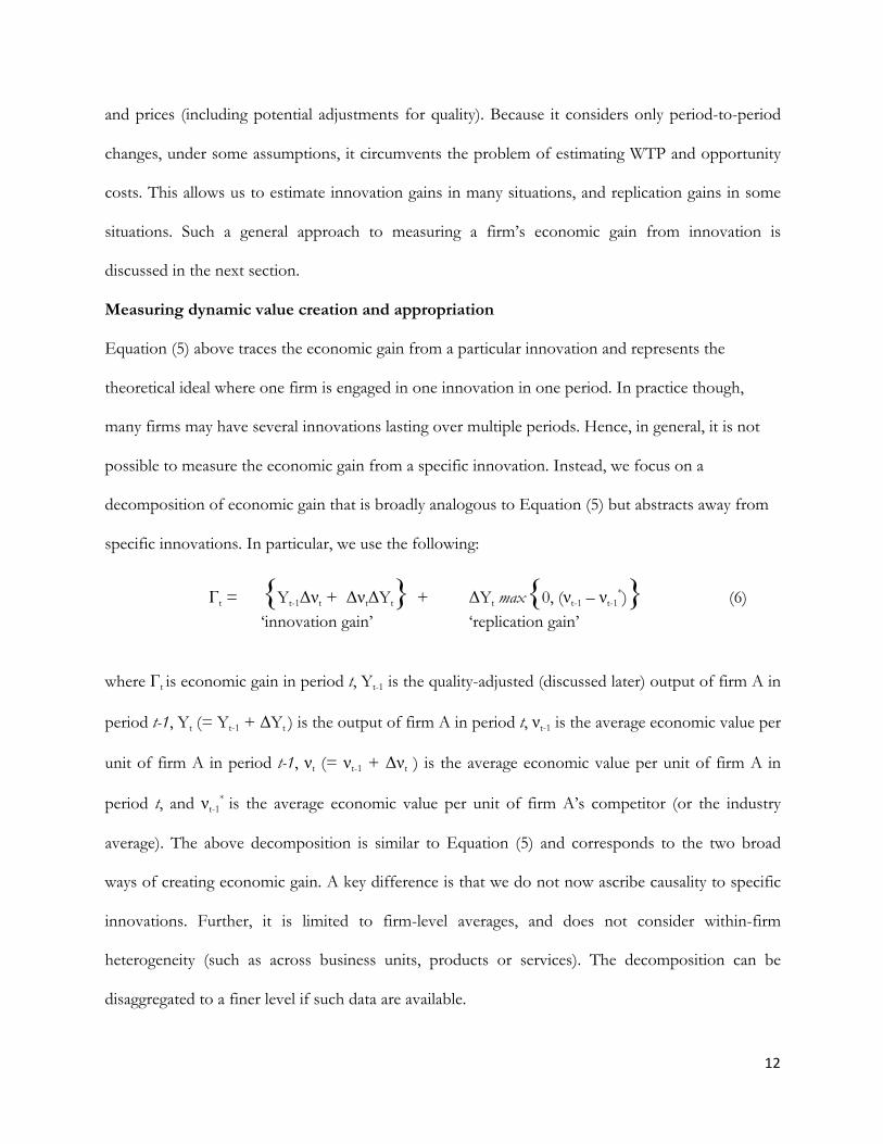
Measuring dynamic value creation and appropriation

Equation (5) above traces the economic gain from a particular innovation and represents the

theoretical ideal where one firm is engaged in one innovation in one period. In practice though,

many firms may have several innovations lasting over multiple periods. Hence, in general, it is not

possible to measure the economic gain from a specific innovation. Instead, we focus on a

decomposition of economic gain that is broadly analogous to Equation (5) but abstracts away from

specific innovations. In particular, we use the following:

Γt = {Yt-1Δνt + ΔνtΔYt} + ΔYt max{0, (νt-1 – νt-1*)} (6)

‘innovation gain’ ‘replication gain’

where Γt is economic gain in period t, Yt-1 is the quality-adjusted (discussed later) output of firm A in

period t-1, Yt (= Yt-1 + ΔYt ) is the output of firm A in period t, νt-1 is the average economic value per

unit of firm A in period t-1, νt (= νt-1 + Δνt ) is the average economic value per unit of firm A in

period t, and νt-1* is the average economic value per unit of firm A’s competitor (or the industry

average). The above decomposition is similar to Equation (5) and corresponds to the two broad

ways of creating economic gain. A key difference is that we do not now ascribe causality to specific

innovations. Further, it is limited to firm-level averages, and does not consider within-firm

heterogeneity (such as across business units, products or services). The decomposition can be

disaggregated to a finer level if such data are available.

13

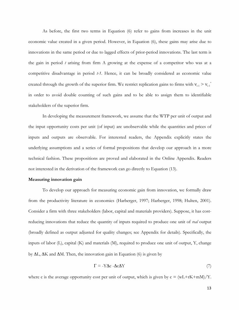
As before, the first two terms in Equation (6) refer to gains from increases in the unit

economic value created in a given period. However, in Equation (6), these gains may arise due to

innovations in the same period or due to lagged effects of prior-period innovations. The last term is

the gain in period t arising from firm A growing at the expense of a competitor who was at a

competitive disadvantage in period t-1. Hence, it can be broadly considered as economic value

created through the growth of the superior firm. We restrict replication gains to firms with νt-1 > νt-1*

in order to avoid double counting of such gains and to be able to assign them to identifiable

stakeholders of the superior firm.

In developing the measurement framework, we assume that the WTP per unit of output and

the input opportunity costs per unit (of input) are unobservable while the quantities and prices of

inputs and outputs are observable. For interested readers, the Appendix explicitly states the

underlying assumptions and a series of formal propositions that develop our approach in a more

technical fashion. These propositions are proved and elaborated in the Online Appendix. Readers

not interested in the derivation of the framework can go directly to Equation (13).

Measuring innovation gain

To develop our approach for measuring economic gain from innovation, we formally draw

from the productivity literature in economics (Harberger, 1997; Harberger, 1998; Hulten, 2001).

Consider a firm with three stakeholders (labor, capital and materials providers). Suppose, it has cost-

reducing innovations that reduce the quantity of inputs required to produce one unit of real output

(broadly defined as output adjusted for quality changes; see Appendix for details). Specifically, the

inputs of labor (L), capital (K) and materials (M), required to produce one unit of output, Y, change

by ΔL, ΔK and ΔM. Then, the innovation gain in Equation (6) is given by

Γ = -YΔc -ΔcΔY (7)

where c is the average opportunity cost per unit of output, which is given by c = (wL+rK+mM)/Y.

14

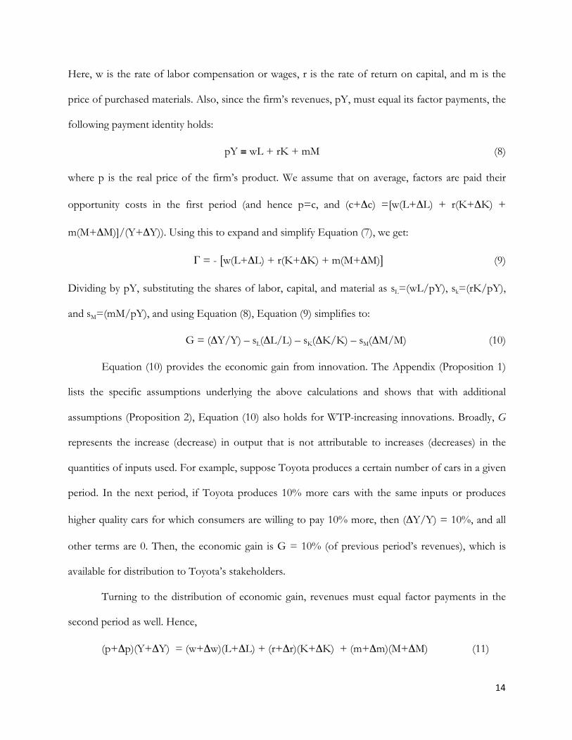
Here, w is the rate of labor compensation or wages, r is the rate of return on capital, and m is the

price of purchased materials. Also, since the firm’s revenues, pY, must equal its factor payments, the

following payment identity holds:

pY ≡ wL + rK + mM (8)

where p is the real price of the firm’s product. We assume that on average, factors are paid their

opportunity costs in the first period (and hence p=c, and (c+Δc) =[w(L+ΔL) + r(K+ΔK) +

m(M+ΔM)]/(Y+ΔY)). Using this to expand and simplify Equation (7), we get:

Γ = - [w(L+ΔL) + r(K+ΔK) + m(M+ΔM)] (9)

Dividing by pY, substituting the shares of labor, capital, and material as sL=(wL/pY), sk=(rK/pY),

and sM=(mM/pY), and using Equation (8), Equation (9) simplifies to:

G = (ΔY/Y) – sL(ΔL/L) – sK(ΔK/K) – sM(ΔM/M) (10)

Equation (10) provides the economic gain from innovation. The Appendix (Proposition 1)

lists the specific assumptions underlying the above calculations and shows that with additional

assumptions (Proposition 2), Equation (10) also holds for WTP-increasing innovations. Broadly, G

represents the increase (decrease) in output that is not attributable to increases (decreases) in the

quantities of inputs used. For example, suppose Toyota produces a certain number of cars in a given

period. In the next period, if Toyota produces 10% more cars with the same inputs or produces

higher quality cars for which consumers are willing to pay 10% more, then (ΔY/Y) = 10%, and all

other terms are 0. Then, the economic gain is G = 10% (of previous period’s revenues), which is

available for distribution to Toyota’s stakeholders.

Turning to the distribution of economic gain, revenues must equal factor payments in the

second period as well. Hence,

(p+Δp)(Y+ΔY) = (w+Δw)(L+ΔL) + (r+Δr)(K+ΔK) + (m+Δm)(M+ΔM) (11)

15

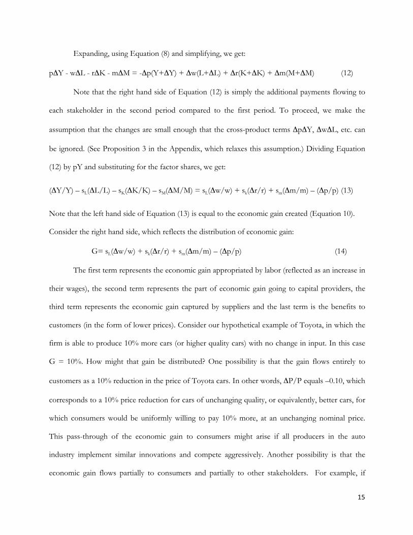
Expanding, using Equation (8) and simplifying, we get:

pΔY - wΔL - rΔK - mΔM = -Δp(Y+ΔY) + Δw(L+ΔL) + Δr(K+ΔK) + Δm(M+ΔM) (12)

Note that the right hand side of Equation (12) is simply the additional payments flowing to

each stakeholder in the second period compared to the first period. To proceed, we make the

assumption that the changes are small enough that the cross-product terms ΔpΔY, ΔwΔL, etc. can

be ignored. (See Proposition 3 in the Appendix, which relaxes this assumption.) Dividing Equation

(12) by pY and substituting for the factor shares, we get:

(ΔY/Y) – sL(ΔL/L) – sK(ΔK/K) – sM(ΔM/M) = sL(Δw/w) + sk(Δr/r) + sm(Δm/m) – (Δp/p) (13)

Note that the left hand side of Equation (13) is equal to the economic gain created (Equation 10).

Consider the right hand side, which reflects the distribution of economic gain:

G= sL(Δw/w) + sk(Δr/r) + sm(Δm/m) – (Δp/p) (14)

The first term represents the economic gain appropriated by labor (reflected as an increase in

their wages), the second term represents the part of economic gain going to capital providers, the

third term represents the economic gain captured by suppliers and the last term is the benefits to

customers (in the form of lower prices). Consider our hypothetical example of Toyota, in which the

firm is able to produce 10% more cars (or higher quality cars) with no change in input. In this case

G = 10%. How might that gain be distributed? One possibility is that the gain flows entirely to

customers as a 10% reduction in the price of Toyota cars. In other words, ΔP/P equals –0.10, which

corresponds to a 10% price reduction for cars of unchanging quality, or equivalently, better cars, for

which consumers would be uniformly willing to pay 10% more, at an unchanging nominal price.

This pass-through of the economic gain to consumers might arise if all producers in the auto

industry implement similar innovations and compete aggressively. Another possibility is that the

economic gain flows partially to consumers and partially to other stakeholders. For example, if

16

Toyota’s rivals do not achieve the same level of economic gain as Toyota—say, because they did not

implement the innovations as successfully—it is likely that only some of Toyota’s gains from

innovations will be competed away to consumers; the remainder may be captured by Toyota’s

employees, suppliers, or shareholders. The extent to which these groups capture Toyota’s overall

gain depends upon their bargaining power, the degree of competition in the industry, and Toyota’s

performance relative to rivals.

Note that the distribution of gains represented by Equation (14) applies even in the absence

of any economic gain by the firm (i.e., when G is zero or even negative). So, some stakeholders

could gain (e.g., consumers) at the expense of other stakeholders (e.g., shareholders), even if the

total economic gain is zero or negative.

In the remainder of this paper, we refer to the formulation represented by Equation (13) [or

its component parts, ‘value creation’ in Equation (10) and ‘value distribution’ in Equation (14)] as

the ‘VCA model’ (for Value Creation and Appropriation). If the production technology is constant

returns to scale, Equation (10) is equivalent to the well-known Solow (1957) decomposition for total

factor productivity (TFP), whereas Equation (14) (the ‘dual’) has been much less frequently used.15

Measuring replication gain

The approach outlined above for measuring economic gain from innovation can be modified to

measure the economic gain from replication. In this case, we first estimate the gain corresponding to

νt-1 – νt-1* in Equation (6), i.e., the gain from shifting a single unit of output from the less efficient

competitor (or industry average) to the focal firm. Then we can multiply this estimate by ΔYt, the

number of units over which the focal firm displaces the competitor.

Suppose the firm faces a competitor with the same WTP as the focal firm, and which pays

15 An exception is Harberger (1997, 1998) and related studies, which apply the TFP formula and the dual to assess economic growth at the industry level.

17

its input owners their opportunity costs. We can then replace the first (baseline) period in the above

discussion with this competitor’s output and inputs scaled in a way that the scaled output matches

the output of the focal firm. Formally, suppose in some period, Yc, Lc, Kc and Mc are the

competitor’s output and input quantities, pc, wc, rc and mc are the output and input prices, and ρ is a

scaling factor such that Yc=ρY1, where Y1 is the output of the focal firm in the first period. Then,

repeating the same calculations as above, we can write:

– {sLc(ΔLc/Lc) + sKc(ΔKc/Kc) + sMc(ΔMc/Mc)} =

sLc(Δwc/wc) + skc(Δrc/rc) + sMc(Δmc/mc) – (Δpc/pc) (15)

Where ΔLc=(ρL1- Lc), ΔKc=(ρK1- Kc), ΔMc=(ρM1- Mc), Δwc=(w1- wc), Δrc=(r1- rc), Δmc=(m1- mc), sLc

= (wcLc/pcYc), sKc = (rcKc/pcYc), and sMc = (mcMc/pcYc). Note that ΔYc=(ρY1- Yc)=0, since we are

scaling the competitor to the firm’s size. Broadly, the left hand side indicates how much more

economic value the firm is creating, per unit of output, relative to the competitor in that period. To

compute replication gains (in dollars) from this period to the next, we multiply throughout by (1/ρ

)pcYc times the extent of growth, (Y2- Y1)/Y1 (Proposition 4 in the Appendix shows this formally).

The right hand side indicates the difference between the two firms in how that economic value is

distributed. In particular, it denotes the additional economic gain (as a percentage of the scaled

competitor’s revenues) to the stakeholders of the superior firm relative to what they would have

received if they were part of the competitor firm in the first period.

AN ILLUSTRATIVE EXAMPLE: SOUTHWEST AIRLINES, 1980-2010

Overview

To illustrate these concepts and methods, we focus on the U.S. airline industry to estimate the

economic gain created by Southwest Airlines (SWA) and American Airlines (AA) over the interval

from 1980 to 2010. We first compare SWA and AA using operational indicators to give an overview

of how value is created in this industry. We then apply the VCA model to develop estimates of

18

economic gain. Our calculations are intended as a quantitative sketch of the creation and distribution

of economic gain by these firms, not as a causal test of any hypotheses.

The airline industry offers several attractive features for applying the VCA model. First, the

requisite data are publicly available for many airline companies over a long period of time. Second,

the industry is likely to meet many of the assumptions required for a reasonable application of the

model. A vast majority of value creation in this industry is through cost-reducing innovations,

particularly with regard to labor and fuel use. Innovation gains through increases in service quality

(higher WTP for a better experience delivered) have been marginal, if any. SWA’s growth has largely

come from a decline in its competitors’ market shares rather than through industry growth. While

there have been improvements in the quality of planes, the quality of other inputs such as fuel and

pilots have not changed significantly. Finally, the industry has been very competitive, which means

the factors are likely to be earning returns close to their opportunity costs.

--Insert Tables 2A and 2B about here--

Tables 2A and 2B summarize the data and our calculations for SWA and AMR over decade

intervals between 1980 and 2010. The US airline industry was deregulated in 1978, when price and

entry restrictions on interstate flights were eliminated. SWA began providing scheduled service in

1971 but remained a small carrier flying only within Texas until late 1979. Thus, our data from 1980

to 2010 capture SWA’s expansion across the United States. In its formative years SWA developed a

distinctive business model (Gittell, 2005), which SWA refined and replicated during the subsequent

period of expansion. By comparison, AA has long been one of the world’s largest airlines; we take

AA as representative of the established carriers in the United States. Moreover, AA and SWA have

always been direct competitors, with SWA headquartered in Dallas, and AA in nearby Fort Worth.

The most common measure of output in the airline industry is ‘revenue passenger miles’

(RPM), the total number of miles flown by paying passengers during a calendar year. We adopt RPM

19

as the standard to compare between the airlines and over time, recognizing that some quality

differences exist.16

SWA is an outlier in the airline industry, having grown to become one of the major carriers

in the United States while remaining consistently profitable. Table 2 shows that in 1980, SWA

produced 7% of AA’s output, based on total RPMs flown. By 2010, SWA had reached almost 60%

of AA’s size and offered service between virtually all of the major cities of the United States. In

1980, SWA’s net income was 13.4% of revenue; by 2010, this ratio had fallen to 3.8%, albeit on a

much larger revenue base. By comparison, AA suffered losses in both years.

The major source of SWA’s advantage has been its labor efficiency. In 1980, SWA had 909

employees per million RPM flown; by 2010, SWA had cut this figure by more than half to 447. In

comparison, AA had 1,526 employees per million RPM in 1980 and 583 in 2010. SWA also enjoyed

an input cost advantage in its early years, given that it paid comparatively low wages and salaries. In

1980, average wages and benefits were just over $26,000 per employee at SWA, as compared with

almost $34,000 at AA. By 2010, however, SWA was paying the highest compensation in the US

airline industry, averaging $106,000 per employee at SWA versus $87,500 at AA. Thus, SWA’s

advantage in labor efficiency was increasingly offset by a higher unit labor cost. In effect, employees

at SWA were capturing a larger share of the value created by the company, as compared with

employees at AA and other legacy carriers.

SWA has enjoyed lesser efficiency advantages in other areas. In 1980, SWA consumed 37 16 Airlines differ across various dimensions of quality. For example, AA offers a mix of coach, business and first class service, whereas SWA provides only coach class. Thus, AA has arguably provided RPMs of higher average quality. On the other hand, SWA’s flights have shorter average length-of-haul, which requires greater resources per RPM (given the time devoted to takeoff and landing). All airlines have adopted tighter packing of passenger seating in recent years, which has reduced the average quality of customer experience, offset to some degree by improvements in other areas such as aircraft entertainment systems. Viewed over a thirty-year perspective, however, such quality-of-service differences are relatively minor, particularly by comparison with many other industries. Thus, RPM provides a reasonably consistent benchmark for assessing value creation across airline companies and over time.

20

gallons of jet fuel per thousand RPM, as compared with 43 gallons at AA. Between 1980 and 2010,

SWA nearly doubled its fuel efficiency while AA improved by an even larger margin; the two carriers

achieved almost identical fuel efficiency in 2010. (These gains stemmed primarily from

improvements made by the aircraft and engine manufacturers.) In most years, SWA appears less

efficient than AA in capital input per RPM, although this could be an accounting issue. In 1980

SWA maintained a significantly higher load factor (RPM divided by Available Seat Miles, or ASM)

than AA; in later years AA achieved marginally higher values than SWA. In general, load factors

have been rising since the 1990s, as airlines have made greater efforts to avoid empty seats. Airlines

have also adopted higher density seating—a fact well known to coach passengers. This tighter

packing of passengers raises efficiency in the use of fuel, capital, materials and labor, although

service quality suffers to a degree.

Estimation of gains to innovation

Table 2a summarizes our estimates of economic gains from innovation at SWA and AA. Applying

Equation (10) to the airline data (after extending the formula to incorporate multiple inputs

including labor, capital, fuel and materials, as described in Authors (2016)), yields the estimated ‘total

gain from innovation’ shown in the bottom portion of the table. In general, innovation gains have

been substantial in the airline industry. Over 1980 to 2010, AA’s percentage gain of 66% exceeded

that of SWA (50%). For both carriers, about half of this total gain arose between 2000 and 2010, a

period of industry restructuring when airlines responded to major pressures, including a deep

recession and a steep rise in oil prices.

Applying Equation (14) to the airline data gives the distribution of the innovation gains

among each firm’s customers, employees, suppliers and shareholders.17 For both airlines, the

17 The analysis can be performed at a more detailed level, e.g., distinguishing management and employee groups within the airlines. Here we focus on average effects by stakeholder category at the expense of a more fine-grained discussion.

21

estimates show a consistent flow of gains to customers, as well as a sharp increase in the value

flowing to fuel suppliers between 2000 and 2010. Employees also captured some of the innovation

gains, although the pattern differs between SWA and AA.

Over the 1980-2010 period, nearly all of AA’s innovation gains were distributed to its

customers in the form of price reductions. This extreme flow of value from AA to customers

reflects the strong competitive pressure in the US airline industry. Only a small proportion (5%) of

AA’s innovation gain went to the company’s employees. Virtually none of the gain went to

shareholders, given that AA experienced losses of about 2% of revenues in both 1980 and 2010.

SWA also distributed the majority of its innovation gains to customers. Relative to AA,

however, SWA’s gains increasingly went to employees. Table 2a shows an employee gain of almost

19% at SWA between 1980 and 2010, more than three times the comparable figure for AA.

Conceivably, this shift of gains to employees at SWA may reflect an effort by the company to

provide incentives and maintain morale needed to sustain rapid growth.

Table 2a reveals shifts of value out of and then returning into the supply chain for fuel, as

fuel prices fell between 1980 and 2000 but then increased more than threefold. Over the period

from 2000 to 2010, the majority of all innovation gains made by SWA and AA flowed to fuel

suppliers, most likely ending up as rents collected by oil producers.

Perhaps surprisingly, Table 2a shows negative gains to capital for SWA. Although seemingly

at odds with SWA’s consistent profitability and rising stock price, the negative values indicate a

decline in the rate of profit, rather than total profit. SWA’s total profit has been increasing, as the

company’s growth more than offset the declining profit rate. Over the 30-year period of our sample,

SWA’s profit rate fell from 13.4% to 3.8% of revenue while the company’s total net income grew

more than sixteen-fold.

22

Gains from replication

The calculations summarized at the bottom of Table 2a estimate the gains from innovation within

SWA and AA as they improved their operations from 1980 to 2010. Complementing this analysis,

Table 2b gives similar calculations that compare between SWA and AA at four points in time: 1980,

1990, 2000 and 2010. These calculations estimate the gains that would have been achieved by

immediately transforming AA into a firm with SWA’s efficiency level. We perform these calculations

by scaling up the data for SWA to match AA’s output (RPM) in each year, and applying Equation

14. Below, we apply these estimates to assess the gains from SWA’s replication and growth.

Table 2b reveals that SWA maintained a significant efficiency advantage over AA in each of

the years examined. However, the magnitude of SWA’s advantage diminished over time. This is

consistent with the higher rates of innovation gain for AA in Table 2a. Based on our calculations,

shifting a unit of output from AA to SWA in 1980 would have produced an economic gain of

27.9%.18 A similar transformation in 2010 yields a gain of only 6.0%. Thus, the efficiency of the two

airlines has been converging over time. One possible explanation is that AA was able to adopt

innovations pioneered by SWA and others at a faster rate than SWA was able to achieve new

innovations to improve its business model.

The bottom portion of Table 2b allows us to draw some tentative inferences about the

distribution of the replication gains made by SWA as it enlarged its market share at the expense of

AA (and other legacy airlines). These calculations suggest that as output and corresponding resource

inputs shifted from AA to SWA, much of the resulting economic gain was distributed to consumers

and shareholders of SWA. This follows directly from the lower prices and higher profits of SWA

relative to AA. However, one needs to be careful about such interpretations, as the calculations are

based upon company averages; we do not know if such a reallocation of resources from AA to SWA 18 Equivalently, AA could have produced its 1980 output with 21.8% (.279/1.279) less resource inputs, based on the factor prices paid by AA in 1980.

23

at the margin would have had the same distribution of returns or have led to the efficiency gains that

we see in Table 2b.

Assessment of overall gains from innovation and replication

To have a complete picture of value creation by SWA, we now bring together the forms of

economic gain discussed in this paper. These are illustrated in Figure 2, which provides a stylized

representation of the US airline industry supply curve as it has shifted over time. To draw this

curve, we assume that AA is representative of all airlines in the industry other than SWA, and that

airlines have constant marginal cost up to capacity. These assumptions imply that the industry

supply curve is made up of an initial flat portion over the output of SWA, followed by a similar

portion at a higher level of resource input for AA and all other airlines. We also ignore any deviation

between the prices of input factors and their opportunity costs, and changes in such over time. The

resulting curve in Figure 2 resembles Figure 1 in the theoretical part of this article.

--Insert Figure 2 about here--

We draw such curves for 1980, 1990, 2000 and 2010 relative to the benchmark of AA’s 1980

cost level (set at 100). The values represented come from SWA’s output and the estimated total

gains from innovation in Tables 2a and 2b. The initial flat portion of the curve is drawn at the level

of SWA’s resource input per RPM, extending horizontally to SWA’s output in each year. The

subsequent portion of the curve is drawn at AA’s resource input per RPM in that year, relative to the

comparable figure in 1980. Hence, in 1980, the portion of the curve corresponding to SWA is

21.8% lower (0.279/1.279, from Table 2b) than the AA part of the curve. These segments shift

downward in each decade at the rates of gain from innovation estimated in Table 2a. The downward

arrows on the left of Figure 2 correspond to the innovation gains of SWA, whereas the downward

arrows on the right of the Figure correspond to the innovation gains of AA. For instance, from 1980

to 1990, SWA’s innovation gain was 5.6% (Table 2a), which corresponds to the length of the top-

24

most downward arrow on the left of Figure 2. The ‘toe’ of the curve expands in each decade, as

SWA’s output has grown.

From these curves in Figure 2 one can gauge magnitudes of ‘static’ and ‘dynamic’ value

creation. In each year, the shaded portion of the curve is the static value creation due to the presence

of SWA in the airline market. It represents SWA’s ‘added value’ to the market, as discussed in the

VBS literature, or equivalently, the loss of value that would arise if SWA did not exist (and its service

was replaced by other, less efficient carriers, as represented by AA). It is clear from the figure that

SWA’s static value-added, given by the area of these rectangles, increased greatly from 1980 to 2000,

as the decline in SWA’s relative efficiency was more than offset by SWA’s growth.19

Figure 2 also illustrates the dynamic economic gains achieved by SWA and AA, which. were

substantial for both companies. The total gain between 1980 and 2010 is the area between the

corresponding supply curves. It is the resource savings achieved through the improvements made

by the two airlines and by the expansion of the more efficient company, SWA.

Limiting the analysis to gains made by SWA, over each decade the total economic gain is

given by the sum of SWA’s innovation gain (denoted by the appropriate downward arrow at the left

of Figure 2 between the supply curves) and SWA’s replication gain (denoted by the horizontal

arrow).20 It is clear that gains from replication have been a large component of SWA’s total

economic gain, given the company’s large initial competitive advantage combined with its rapid

growth. Indeed, if SWA had made innovation gains at its historic rate without expanding from its

1980 level of output, the company’s total economic gain would have been meager—merely the small

rectangle between the y-axis and the downward arrows shown for SWA. 19 Under the assumptions, SWA’s static value creation (or value added) in each year equals SWA’s efficiency differential, as indicated in Table 2B, times the output of SWA in that year. 20 If AA is also innovating, another reasonable estimate of SWA’s replication gain would net out the economic gain associated with AA’s innovation from SWA’s replication gain. However, then AA’s gains cannot be mapped to its stakeholders in that period (because the output and inputs associated with those gains is within SWA). The Online Appendix discusses this further.

25

DISCUSSION

We now consider some implications of the VCA Model, and the advantages and limitations of the

measurement framework. We conclude with a brief discussion of areas for future research.

Implications of the VCA Model in Linking Value Creation and Distribution

Lack of correspondence between creation and capture of economic gain. The VCA Model requires that the

economic gain must be equal to the sum of the gains appropriated by the various stakeholders, but it

does not impose any restrictions on how much each individual stakeholder can appropriate. This

lack of a value creation–appropriation correspondence is similar to that in the VBS literature

(Brandenburger and Stuart, 1996; MacDonald and Ryall, 2004) where value appropriation is

indeterminate, subject to bounds. Furthermore, recent advances in strategic management, including

works on the dynamics of rent appropriation and stakeholder bargaining power (Coff, 1999;

Castanias and Helfat, 2001; Lippman and Rumelt, 2003a,b; Asher, Mahoney, and Mahoney, 2005;

Wang and Barney, 2006; Coff, 2010; Harrison, Bosse, and Phillips, 2010), are consistent with this

intuition. These properties allow a simultaneous examination of value creation and appropriation in

empirical studies. Such an exercise is not possible with shareholder value, which, by definition,

equals the value appropriated by the shareholders.

Lack of correspondence between profit growth and economic gain. Profit growth is a key objective for managers

and shareholders. However, profit growth does not correspond to economic gain if it comes at the

expense of another stakeholder’s returns. As can be seen from Equation (14), such cases represent

value transfers from one stakeholder to another rather than value creation. Conversely, while an

increase in competitive advantage leads to economic gain, such a gain does not necessarily translate

into profit growth. Competition for resources and customers may result in all economic gain created

by the firm being competed away to customers and resource owners. Hence, profit growth does not

imply positive economic gain, and conversely, positive economic gain does not imply profit growth.

26

Innovation gain and the average unit stakeholder returns. Innovation is often considered critical to a firm’s

performance. Our framework highlights another important aspect of innovation: only innovation

gain can increase the average unit stakeholder returns for all stakeholders of a given firm. To see this,

set the left hand side of Equation (14) to zero. Then, if one stakeholder gains, at least one other

stakeholder must lose.

By comparison, pure replication is simply scaling up the current level of value creation by

proportionately expanding the firm’s inputs and outputs. Hence, while the total level of value

creation goes up, the value created per unit does not change, which in turn implies that the average

return for all stakeholders cannot increase. This does not mean that the firm’s stakeholders do not

gain. Because the firm is expanding, it will have more employees, customers and suppliers, who in

aggregate now receive more economic value than they did previously (e.g., when they were

associated with the firm’s competitors). Hence, some or all of these stakeholders clearly benefit from

replication gain, even though the average return may not change.

Advantages and Limitations of the VCA model

A major advantage of the VCA model, besides its tight integration with theory, is that the data

required for estimating Equation 13 (quantities and prices of inputs and outputs) are publicly

available for many firms and industries. Furthermore, the model is based on a payment identity and

thus does not require that markets be in some form of equilibrium. The method is therefore widely

applicable.

Even so, the full set of required prices and quantities are not obtainable for many firms and

industries. Data on inputs from suppliers are normally lacking. In such cases, an abbreviated form of

the model can be estimated based on value-added, as we discuss in Lieberman et al. (2016). A related

constraint is that most US companies do not provide data on employee wages and benefits, and

some companies are diversified to an extent that makes it hard to untangle value creation within

27

specific businesses without access to detailed business-unit data. Still, an exploratory analysis of the

Compustat Global database (which covers 1996-2010 and about 115 countries) suggests that there

are well over 87,000 firm-year observations with all the required data. The Online Appendix

provides additional details, including data availability by country and by industry sector, and a flow

chart that helps assess whether our model may be suitably applied.

Another advantage of the model is its relation to traditional measures of firm performance,

such as return on assets. Ignoring taxes, our measure of the gains to capital (sk Δr/r) represents the

part of the economic gain that flows to shareholders. For instance, consider a firm with a capital (K)

of 250 million dollars, and initial revenue (pY) of $200 million, of which $75 million went to workers

as wages and benefits (wL), $25 million as profits to capital (rK), and $100 million as payments to

suppliers. Then, its initial return on assets, r, would be 10%. If this firm creates an economic gain of

2%, then without any change in output prices, employment, wages, or capital stock, the measure, sk

Δr/r, would be 2%, since capital owners capture all the economic gain. The new return on assets can

be obtained by adding the incremental $4 million (2% of $200 million) to profits, and dividing by the

capital base to get 11.6%.21 Hence, gains to capital in the model will be correlated with increased

return on assets as measured traditionally. Nevertheless, as the SWA example demonstrates, one

must be careful not to view a declining rate of return as necessarily indicative of a decline in the

firm’s economic profits. For growing firms whose returns exceed the cost of capital, economic

profits can increase despite a diminishing rate of return.

While the VCA model has wide applicability, many limitations must be recognized. We now

elaborate on these, referring the reader to Lieberman et al. (2016) for further details on some

context-specific issues.

21 Part of this return represents depreciation; if the rate of economic depreciation is 10%, the return net of depreciation is initially zero, rising to 1.6% in the second period.

28

At the outset, note that we are using the terms ‘innovation’ and ‘replication’ to mean specific

types of economic gain attributable to firm-level changes. We are agnostic, however, about the

nature of underlying sources. Innovation gain could be due to the firm’s own innovation or to

imitation of rivals or some other form of spillovers. Similarly, replication gain is the additional

economic value created in a given period because the firm expanded by displacing a competitor who

was less efficient in the prior period. In our framework, the economic gain created by a firm through

imitation of a competitor’s innovation would be first reflected as an innovation gain for the imitating

firm; subsequently, this firm might be able to grow and displace other competitors who failed to

adopt the innovation, leading to what we call replication gain. Indeed, the biggest creator of value in

an industry is often not the original innovator. If the objective is to separate economic gain into

‘innovation’ and ‘replication’ as defined in this article, then our framework will provide the correct

breakdown, within the bounds of its assumptions. This also means that our framework is not a

causal framework.

If market shares remain stable over time, all economic gains in an industry will take the form

of innovation gain. However, as the example of SWA illustrates, in some cases a firm’s total

economic gain may be achieved largely through displacement of competitors. In such instances it is

important to account for replication gain, even though the estimate of this gain is sensitive to

assumptions with respect to the identity of the competitor(s) being displaced. In our airline example

we took AA as a representative competitor, but alternatively, we could have taken an average of

multiple airlines or have based our calculations on the actual changes in airline market shares

observed in each period.

As shown in the Appendix and Online Appendix, the VCA framework exactly measures the

innovation gains under certain assumptions. The Online Appendix provides propositions and a

simulation analysis of the potential direction and magnitude of distortion if these assumptions are

29

not met. More importantly, it helps develop a broad idea of contexts where our framework is likely

to be reasonably accurate. We summarize findings from those analyses here.

In general, we find that the framework does well in measuring innovation gain if the firm

grows by displacing competitors through cost-reducing innovations, and when input factors are not

paid significantly more than their opportunity costs (Proposition 1 in the Appendix, Baseline

Scenario and Scenario 2 in the Online Appendix). This is true even for large innovations that result

in significant firm growth. Such conditions broadly match the assumptions of Solow’s (1957) classic

article and the literature on TFP (Hulten, 2001). Thus, established industries where cost-reducing

innovations are the predominant form of innovation are likely to be particularly good contexts for

applying the model. Airlines are one such example.

With WTP-increasing innovations, in theory, the model requires a constant-quality price

index that reflects the underlying quality changes at the firm level. (See Proposition 2 in the

Appendix.) While such firm-specific price indexes can be developed, a reasonable alternative is the

use of industry-level constant-quality price indexes. Such indexes have been studied extensively (see

for example, Diewert, 1995) and are readily available for many industries (see Online Appendix for a

list). However, the use of such an industry-level price index requires the assumption that any

observed price differences across firms in the same industry reflect quality differences (see

Propositions 7—9 in the Online Appendix). This is more likely to be true for persistent long-term

price differences than for short-term differences. It may be problematic for short-run analyses in

very competitive industries with large inter-firm quality differences, where firms may pass through

part or all of their quality advantage to consumers in the form of lower prices. Hence, a structural

approach may be more appropriate to evaluate value creation and distribution in such contexts (e.g.,

Grennan, 2014). Similar measurement issues also arise if real input quantities are not directly

30

observed or if we cannot completely adjust for input quality changes (see Proposition 6 in the

Online Appendix).

Another source of measurement error is deviations of input prices from opportunity costs in

the first period, which may arise if factor markets are not competitive. Though the framework allows

for inter-supplier heterogeneity within a class of input providers, it assumes that on average, input

providers are paid their opportunity costs in the first period. Sensitivity to this issue is discussed in

the Online Appendix (Proposition 5 and Scenario 2 in the simulation analysis). In general, if a factor

(such as labor) is paid more than its opportunity cost in the first period, the innovation gain arising

from any savings of that factor per unit of output in the second period will be overestimated.

Significant industry innovation may result in the addition of new customers to the industry.

This may overestimate true innovation gain for a specific firm. Broadly, output sold to these new

customers has a lower economic value per unit than output sold to the industry’s existing customers,

which the VCA model is not able to discriminate.22

Another important limitation is that the method uses the marginal customer as a proxy for all

customers. Thus, our approach ignores the fact that benefits to ‘infra-marginal customers’ (i.e.,

customers whose WTP is greater than the price) may differ from the marginal customer. This may

be particularly problematic if a certain innovation increases the WTP for some customers but not

for others. Further, any economic gain created through a unit-for-unit substitution of a costlier input

(i.e., an input with higher opportunity costs) with a cheaper input (i.e., an input with lower

opportunity costs) is not measured.

It is important to note that the choice of endpoints in performing the calculation can be

critical; selection of endpoints that are at different stages of a business cycle can introduce serious

22 However, as shown in the Online Appendix, the magnitude of such error is likely to be large only in industries where demand is highly elastic. In other industries with low to moderate price elasticity, the framework is likely to reasonably approximate actual innovation gains in industries.

31

distortion. Furthermore, Divisia indexes, such as Equation 13, are path dependent (Hulten, 1973).

Hence an aggregation of sequential annual estimates will yield different values than when two distant

endpoints are compared directly. Star and Hall (1976) suggest that such deviations tend to be small,

but further work is needed to explore how these issues affect the robustness of estimates based on

the VCA model.

Finally, the model relies heavily on accounting-based measures. Previous research has

identified inherent limitations of accounting data to measure anything of economic relevance

(Benston, 1985; Fisher & McGowan, 1983). Accounting measures generally ignore the time value of

money and can be distorted by depreciation schedules, variations in investments periods, or

differential growth rates, which may cause the accounting rate of return to deviate from the

economic rate of return (Fisher & McGowan, 1983).23

Notwithstanding these limitations, Equation 13’s usefulness lies in its ability to provide

quantitative insights into the distribution of value among the firm’s stakeholders. None of the

current methodologies used in the strategic management field offer such a possibility, which has

constrained quantitative investigations of questions related to value appropriation. The limitations

discussed above only serve as reminders to be careful when interpreting the results.

Areas for future research

The VCA model offers many potential future research avenues, particularly for empirical

studies. We suggest a few examples. Note that the model is agnostic about the underlying source of

economic gain, and hence, is not by itself a causal framework. Even so, estimates from the

framework can be used to study causal hypotheses, under the same condition required for any 23 Although we cannot fully overcome these problems, our approach runs parallel to work in Productivity Accounting, a fruitful area of research which blends economics, statistics and business performance metrics (Davis, 1955; Grifell-Tatjé & Lovell, 2015). Recent studies in this research tradition have been able to obtain firm-level productivity estimates by using accounting data combined with supplementary information on input/output quantities and price indexes (e.g., Brea-Solís, Casadesus-Masanell, & Grifell-Tatjé, 2015).

32

empirical study in strategy: there is some exogenous variation in the data that permits causal

identification.24

One issue that can be explored is whether shareholders are better positioned to capture gains

from innovation or from replication. Replication gains do not usually require a firm to introduce

changes in its business model. The firm simply grows by replacing less efficient competitors. Hence,

there are no new knowledge asymmetries (in the sense of Coff, 2010) that stakeholders can exploit

to capture more rents. Innovation gains typically require the efforts of skilled employees, who may

capture a larger share of those gains. Hence, we conjecture that shareholders, as residual claimants,

capture relatively more of replication gains (compared to innovation gains). This is consistent with

the evidence for SWA (comparing Tables 2a and 2b).25

Similarly, the model can be used to examine if a more ‘equitable’ distribution of economic gain

helps or hinders overall firm growth and the sustainability of a firm’s competitive advantage. A

number of literatures suggest that a broad sharing of economic gains is beneficial to the firm’s

stakeholders (including shareholders) over the long term (Harrison, Bosse, and Phillips, 2010;

Weitzman, 1984). Similarly, Coff (1999) suggested that if shareholders do not appropriate value (or

their appropriation is not evident in accounting performance), it might limit imitation attempts since

the firm might not appear to be unusually profitable. More generally, the division of the economic 24 We conjecture that assumptions regarding the time lag between the timing of an innovation and its impact on the average willingness to pay-cost gap and output growth (somewhat similar to assumptions in productivity estimation techniques such as Ackerberg-Caves-Frazer (2015) that assume a time lag between the firm’s productivity changes and the change in input quantities, which allows them to causally estimate productivity) may be helpful. We leave this topic for future research. 25 A related question relates to how the rate of growth may affect the ability of employees to capture economic gains. Compared with other factors utilized by the firm, skilled labor may be the more difficult to increase rapidly and effectively. If new workers cannot be hired and trained quickly, current employees may require incentives, e.g., to work overtime or to ensure their long-term retention within the firm. Moreover, employees may have power (through unions or other mechanisms) to impede the growth process. A firm that is growing rapidly may therefore choose to pay a premium to its workers. Conversely, a firm that is shrinking and laying off workers may have power to shift economic gains increasingly to shareholders.

33

pie can affect the future size of the pie. Potentially, these ideas can be empirically assessed in the

VCA framework.

CONCLUSION

Understanding value creation and appropriation in firms has been one of the most fundamental

concerns of the field of strategic management. Even so, the field has lacked clear definitions of value

creation, and the extant approaches to measurement have important limitations. In this article we

have attempted to provide greater clarity on the definitions by highlighting two main dimensions of

misunderstanding—the breadth of stakeholder(s) being considered (shareholders vs. others) and the

timeframe for analysis (static or within a single period, vs. dynamic across periods). We have focused

on dynamic value creation and introduced the concept of economic gain: the increase in economic

surplus generated by the firm between one time period and another. Furthermore, we have

illustrated two main ways of creating economic gain—through innovations that reduce costs or

increase WTP, and through the growth and replication of superior firms. Finally, we have presented

a general, flexible, and computationally feasible method to estimate economic gain and its

distribution among the firm’s stakeholders. We hope these efforts bring greater precision to the

definition of value creation and provide a useful foundation for measurement in future research.

REFERENCES Ackerberg D, Benkard CL, Berry S, Pakes A. 2007. Econometric Tools for Analyzing Market

Outcomes. Handbook of Econometrics 6 (Part A): 4171–4276. Ackerberg D. Caves K, Frazer G. Identification Properties of Recent Production Function

Estimators, Econometrica 83: 2411-2451 Asher CC, Mahoney JM, Mahoney JT. 2005. Towards a Property Rights Foundation for a

Stakeholder Theory of the Firm. Journal of Management and Governance 9: 5–32. Barney JB. 1991. Firm Resources and Sustained Competitive Advantage. Journal of Management 17: 99. Bennett VM. 2013. Organization and Bargaining: Sales Process Choice at Auto Dealerships.

Management Science 59(9): 2003-2018. Benston GJ. 1985. The Validity of Profit-Structure Studies with Particular Reference to the FTC’s

Line of Business Data. American Economic Review 75(1): 37. Besanko D, Dranove D, Schaefer S, Shanley M. 2010. Economics of Strategy (6th ed.). John Wiley &

Sons: New York.

34

Blair MM. 1998. For Whom Should Corporations Be Run?: An Economic Rationale for Stakeholder Management. Long Range Planning 31(2): 195–200.

Bowman C, Ambrosini V. 2003. How the Resource-based and the Dynamic Capability Views of the Firm Inform Corporate-level Strategy. British Journal of Management 14(4): 289-303.

Brandenburger AM, Stuart H. 1996. Value-Based Business Strategy. Journal of Economics and Management Strategy 5: 5–25.

Brea-Solís H, Casadesus-Masanell R, Grifell-Tatjé E. 2015. Business Model Evaluation: Quantifying Walmart’s Sources of Advantage. Strategic Entrepreneurship Journal 9(1): 12-33.

Castanias RP, Helfat CE. 2001. The Managerial Rents Model: Theory and Empirical Analysis. Journal of Management 27: 661–678.

Chatain O, Zemsky P. 2011. Value Creation and Value Capture with Frictions. Strategic Management Journal 32(11): 1206-1231.

Coff RW. 1999. When Competitive Advantage Doesn’t Lead to Performance: The Resource-Based View and Stakeholder Bargaining Power. Organization Science 10(2): 119–133.

Coff RW. 2010. The Coevolution of Rent Appropriation and Capability Development. Strategic Management Journal 31: 711–733.

Davis E, Kay J. 1990. Assessing Corporate Performance. Business Strategy Review 1: 1. Davis HS. 1955. Productivity accounting. University of Pennsylvania Press: Philadelphia. Diewert, W.E., 1995. Axiomatic and Economic Approaches to Elementary Price Indexes. Working

Paper. National Bureau of Economic Research Donaldson T, Preston LE 1995. The Stakeholder Theory of the Corporation: Concepts, Evidence,

and Implications. The Academy of Management Review 20(1): 65-91. Fisher FM, McGowan JJ. 1983. On the Misuse of Accounting Rates of Return to Infer Monopoly

Profits. American Economic Review 73(1): 82. Garcia-Castro R, Aguilera RV. 2015. Incremental value creation and appropriation in a world with

multiple stakeholders. Strategic Management Journal 36(1): 137-147. Gittell JH. 2005. The Southwest Airlines way. McGraw-Hill: New York. Grennan M. 2014. Bargaining Ability and Competitive Advantage: Empirical Evidence from Medical

Devices. Management Science 60(12): 3011-3025. Grifell-Tatjé E, Lovell CAK. 2015. Productivity Accounting: The Economics of Business Performance.

Cambridge University Press: New York. Harberger AC. 1954. Monopoly and resource allocation, American Economic Review, 44(2): 77-87. Harberger AC. 1964. The measurement of waste, American Economic Review, 54(3): 58-76. Harberger AC. 1971. Three Basic Postulates for Applied Welfare Economics. Journal of Economic

Literature 9(3): 785–797. Harberger AC. 1998. A Vision of the Growth Process. American Economic Review 88: 1–32. Harberger AC. 1997. Studying the Growth Process: A Primer. Paper prepared for a conference on

Capital Formation and Economic Growth at The Hoover Institution, Stanford University Harrison JS, Bosse DA, Phillips RA. 2010. Managing for Stakeholders, Stakeholder Utility Functions,

and Competitive Advantage. Strategic Management Journal 31(1): 58–74. Hines JR. 1998. Three sides of Harberger Triangles, NBER Working Paper 6852. Hulten CR. 1973. Divisia Index Numbers. Econometrica 41(6): 1017–1025.

35

Hulten CR. 2001. Total Factor Productivity: A Short Biography. In National Bureau of Economic Research, Hulten, C.R, Dean, E.R., and Harper, M.J. (eds). University of Chicago Press:Chicago, IL.: 1-54.

Jonsson A, Foss NJ. 2011. International expansion through flexible replication: Learning from the internationalization experience of IKEA. Journal of International Business Studies 42(9): 1079-1102.

Kahneman D. 2011. Thinking Fast and Slow. Farrar, Strauss and Giroux: New York. Lieberman MB, Garcia-Castro R, Balasubramanian N. 2016. Measuring Value Creation and

Appropriation in Firms: The VCA Model. Strategic Management Journal (Forthcoming). Lippman SA, Rumelt RP. 2003a. The Payments Perspective: Micro-Foundations of Resource

Analysis. Strategic Management Journal 24: 903–927. Lippman SA, Rumelt RP. 2003b. A Bargaining Perspective on Resource Advantage. Strategic

Management Journal 24: 1069–1086. Luffman GA, Wit SF, Lister S. 1982. A Quantitative Approach to Stakeholder Interests. Managerial

& Decision Economics 3: 70–78. Macdonald G, Ryall RD. 2004. How Do Value Creation and Competition Determine Whether a

Firm Appropriates Value? Management Science 50: 1319-1333. Makadok R. 2011. The Four Theories of Profit and Their Joint Effects. Journal of Management 37(5):

1316-1334. Makadok R, Coff RW. 2002. The theory of value and the value of theory: Breaking new ground

versus reinventing the wheel. Academy of Management Review 27(1): 10-13. Peteraf MA, Barney JB. 2003. Unraveling the Resource-Based Tangle. Managerial & Decision Economics

24: 309–323. Porter, ME. 1985. Competitive Advantage. Free Press: New York. Solow R. 1957. Technical Change and the Aggregate Production Function. Review of Economics and

Statistics 39: 312–320. Star S, Hall RE. 1976. An Approximate Divisia Index of Total Factor Productivity. Econometrica

44(2): 257-263. Stuart HW. 2007. Creating monopoly power. International Journal of Industrial Organization 25(5):

1011-1025. Wang HC, Barney JB. 2006. Employee Incsentives to make Firm-Specific Investments: Implications

for Resource-Based Theories of Corporate Diversification. Academy of Management Review 31: 466–476.

Weitzman M. 1984. The share economy. Harvard University Press: Cambridge, MA. Wernerfelt B. 1984. A Resource-Based View of the Firm. Strategic Management Journal 5: 171-180. Winter SG, Szulanski G. 2001. Replication as Strategy. Organization Science 12(6): 730-743.

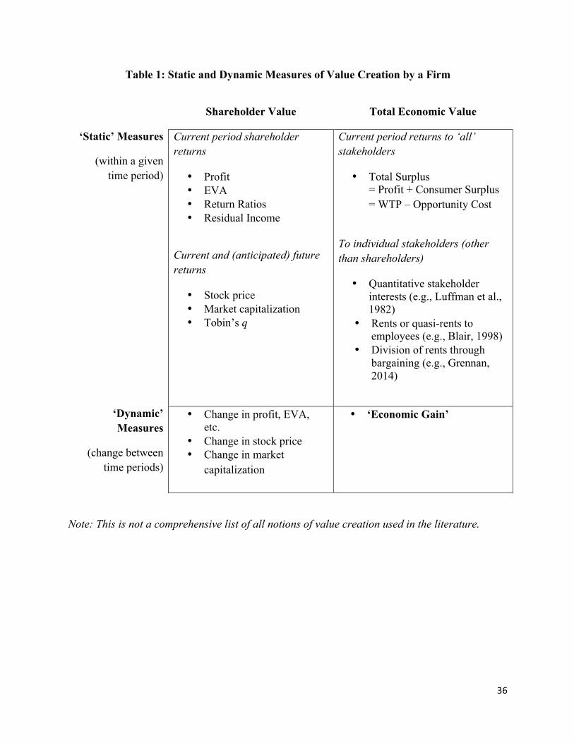
36

Table 1: Static and Dynamic Measures of Value Creation by a Firm

Shareholder Value Total Economic Value

‘Static’ Measures

(within a given time period)

Current period shareholder returns

• Profit • EVA • Return Ratios • Residual Income

Current and (anticipated) future returns

• Stock price • Market capitalization • Tobin’s q

Current period returns to ‘all’ stakeholders

• Total Surplus = Profit + Consumer Surplus = WTP – Opportunity Cost

To individual stakeholders (other than shareholders)

• Quantitative stakeholder interests (e.g., Luffman et al., 1982)

• Rents or quasi-rents to employees (e.g., Blair, 1998)

• Division of rents through bargaining (e.g., Grennan, 2014)

‘Dynamic’ Measures

(change between time periods)

• Change in profit, EVA, etc.

• Change in stock price • Change in market

capitalization

• ‘Economic Gain’

Note: This is not a comprehensive list of all notions of value creation used in the literature.

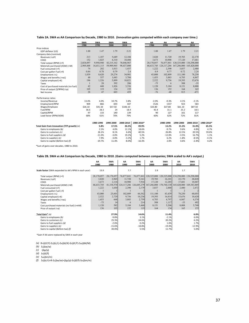
37

Table2A.SWAvsAAComparisonbyDecade,1980to2010.(Innovationgainscomputedwithineachcompanyovertime.)SWA SWA SWA SWA AA AA AA AA1980 1990 2000 2010 1980 1990 2000 2010

1.00 1.47 1.79 2.21 1.00 1.47 1.79 2.21

Revenues(=pY) 213 1,187 5,649 12,104 3,820 11,720 19,703 22,170COGS 152 1,025 4,310 10,488 3,673 10,908 17,120 17,681

2,024,097 9,958,940 42,215,162 78,046,967 28,178,057 76,877,841 120,325,000 134,298,0002,969,448 16,411,115 59,909,965 98,437,000 46,633,745 124,117,286 167,286,000 165,420,000

74 282 1,013 1,437 1,222 2,390 3,037 2,4800.84 0.78 0.79 2.4 0.9 0.77 0.72 2.241,839 8,620 29,274 34,901 43,000 102,809 111,100 78,25048 357 1,683 3,704 1,453 3,883 6,783 6,847196 1,326 5,899 10,821 2,522 9,756 19,393 15,676

Taxes 1 28 392 286 -75 6 508 -3542 448 1,826 3,336 1,120 5,184 8,151 8,008105 119 134 155 136 152 164 16528 47 603 459 -76 -40 813 -471

13.4% 4.0% 10.7% 3.8% -2.0% -0.3% 4.1% -2.1%909 866 693 447 1526 1337 923 583

$26.10 $41.50 $57.50 $106.10 $33.80 $37.80 $61.10 $87.50Fuel/RPM 36.6 28.3 24 18.4 43.4 31.1 25.2 18.5

97 133 140 139 90 127 161 11768% 61% 70% 79% 60% 62% 72% 81%

1980-1990 1990-2000 2000-2010 1980-2010* 1980-1990 1990-2000 2000-2010 1980-2010*TotalGainfromInnovation(TFPgrowth)(a) 5.8% 17.5% 26.5% 49.9% 13.2% 21.3% 31.0% 65.5%

Gainstoemployees(b) 2.5% 4.0% 12.1% 18.6% -9.7% 9.6% 4.8% 4.7%Gainstocustomers(c) 26.1% 8.1% 6.6% 40.5% 26.8% 12.5% 20.5% 59.6%Gainstofuelsuppliers(d) -11.0% -3.0% 19.2% 5.2% -12.0% -3.5% 16.7% 1.1%Gainstosuppliers(e) 7.9% -3.0% -3.2% 1.7% 6.2% -1.8% -8.5% -4.1%Gainstocapital(Before-tax)(f) -19.7% 11.4% -8.0% -16.3% 2.0% 4.6% -2.4% 4.2%

Table2B.SWAvsAAComparisonbyDecade,1980to2010.(Gainscomputedbetweencompanies;SWAscaledtoAA'soutput.)

AA SWA AA SWA AA SWA AA SWA1980 1980 1990 1990 2000 2000 2010 2010

13.9 7.7 2.9 1.7

28,178,057 28,178,057 76,877,841 76,877,841 120,325,000 120,325,000 134,298,000 134,298,000Revenues(=pY) 3,820 2,965 11,720 9,161 19,703 16,101 22,170 20,828COGS 3,673 2,116 10,908 7,916 17,120 12,285 17,681 18,047

46,633,745 41,338,570 124,117,286 126,685,279 167,286,000 170,760,130 165,420,000 169,383,8051,222 1,030 2,390 2,179 3,037 2,888 2,480 2,472

1 1 1 1 1 1 2 243,000 25,601 102,809 66,542 111,100 83,439 78,250 60,0552,522 2,729 9,756 10,236 19,393 16,814 15,676 18,6201,453 668 3,883 2,759 6,783 4,797 6,847 6,374

Taxes -75 14 6 214 508 1,117 -35 492Costpurchasedmaterials(nofuel)(=mM) 1,120 582 5,184 3,460 8,151 5,206 8,008 5,740

136 105 152 119 164 134 165 155

27.9% 14.6% 11.4% 6.0%-9.8% 3.1% -2.1% 6.0%25.3% 24.6% 20.2% 6.2%-2.0% 0.2% 1.0% 1.7%-15.6% -18.8% -19.4% -12.9%30.0% 5.5% 11.7% 5.0%

(a) R=(∆Y/Y)-SL(∆L/L)-SK(∆K/K)-SF(∆F/F)-SM(∆M/M)(b) SL(∆w/w)(c) -(∆p/p)(d) SF(∆f/f)(e) SM(∆m/m)(f) SK(∆r/r)=R-SL(∆w/w)+(∆p/p)-SF(∆f/f)-SM(∆m/m)

Gainstosuppliers(e)Gainstocapital(Before-tax)(f)

*GainifAAwerereplacedbySWAineachyear

*Sumofgainsoverdecades,1980to2010.

Priceofoutput(=p)

TotalGain*(a)Gainstoemployees(b)Gainstocustomers(c)Gainstofuelsuppliers(d)

Materialspurchased(ASM)(=M)Fuelconsumed(=F)CostpergallonFuel(=f)Employment(=L)Capitalemployed(=K)Wagesandbenefits(=wL)

Loadfactor(RPM/ASM)

Scalefactor(SWAexpandedtoAA'sRPMineachyear)

Totaloutput(RPM)(=Y)

NetIncome

PerformanceratiosIncome/RevenueEmployment/RPMWages/Employee

Capital/RPM

Priceofoutput($/RPM)(=p)

PriceindicesGDPdeflator(US)

Companydata(nominal)

Totaloutput(RPM)(=Y)Materialspurchased(ASM)(=M)Fuelconsumed(=F)CostpergallonFuel(=f)Employment(=L)Wagesandbenefits(=wL)Capitalemployed(=K)

Costofpurchasedmaterials(nofuel)

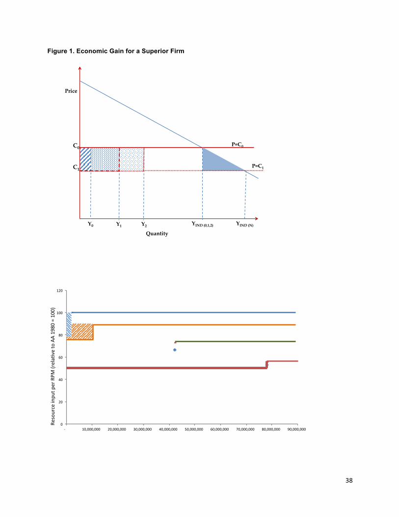
38

Figure 1. Economic Gain for a Superior Firm

Y0

Quantity

Price

P=C0

Y1 Y2

C1

YIND (0,1,2)

P=C1

YIND (N)

C0

0

20

40

60

80

100

120

- 10,000,000 20,000,000 30,000,000 40,000,000 50,000,000 60,000,000 70,000,000 80,000,000 90,000,000

Resourceinpu

tperRPM

(rela>

veto

AA1980=100)

Output=RevenuePassengerMiles(RPM)

1980

1990

2000

2010

Figure2.ValueCreatedbySWAThroughInnova;onandReplica;on,1980to2010

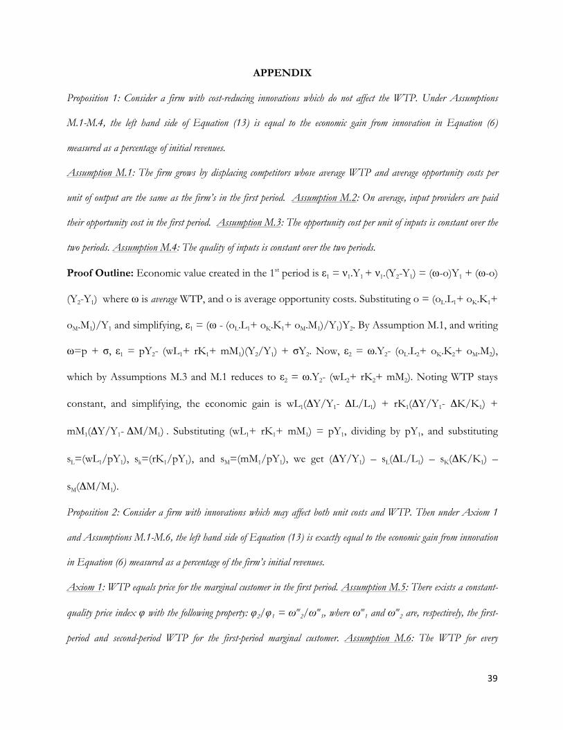
39

APPENDIX

Proposition 1: Consider a firm with cost-reducing innovations which do not affect the WTP. Under Assumptions

M.1-M.4, the left hand side of Equation (13) is equal to the economic gain from innovation in Equation (6)

measured as a percentage of initial revenues.

Assumption M.1: The firm grows by displacing competitors whose average WTP and average opportunity costs per

unit of output are the same as the firm’s in the first period. Assumption M.2: On average, input providers are paid

their opportunity cost in the first period. Assumption M.3: The opportunity cost per unit of inputs is constant over the

two periods. Assumption M.4: The quality of inputs is constant over the two periods.

Proof Outline: Economic value created in the 1st period is ε1 = ν1.Y1 + ν1.(Y2-Y1) = (ω-o)Y1 + (ω-o)

(Y2-Y1) where ω is average WTP, and o is average opportunity costs. Substituting o = (oL.L1+ oK.K1+

oM.M1)/Y1 and simplifying, ε1 = (ω - (oL.L1+ oK.K1+ oM.M1)/Y1)Y2. By Assumption M.1, and writing

ω=p + σ, ε1 = pY2- (wL1+ rK1+ mM1)(Y2/Y1) + σY2. Now, ε2 = ω.Y2- (oL.L2+ oK.K2+ oM.M2),

which by Assumptions M.3 and M.1 reduces to ε2 = ω.Y2- (wL2+ rK2+ mM2). Noting WTP stays

constant, and simplifying, the economic gain is wL1(ΔY/Y1- ΔL/L1) + rK1(ΔY/Y1- ΔK/K1) +

mM1(ΔY/Y1- ΔM/M1) . Substituting (wL1+ rK1+ mM1) = pY1, dividing by pY1, and substituting

sL=(wL1/pY1), sk=(rK1/pY1), and sM=(mM1/pY1), we get (ΔY/Y1) – sL(ΔL/L1) – sK(ΔK/K1) –

sM(ΔM/M1).

Proposition 2: Consider a firm with innovations which may affect both unit costs and WTP. Then under Axiom 1

and Assumptions M.1-M.6, the left hand side of Equation (13) is exactly equal to the economic gain from innovation

in Equation (6) measured as a percentage of the firm’s initial revenues.

Axiom 1: WTP equals price for the marginal customer in the first period. Assumption M.5: There exists a constant-

quality price index φ with the following property: φ2/φ1 = ωm2/ωm

1, where ωm1 and ωm

2 are, respectively, the first-

period and second-period WTP for the first-period marginal customer. Assumption M.6: The WTP for every

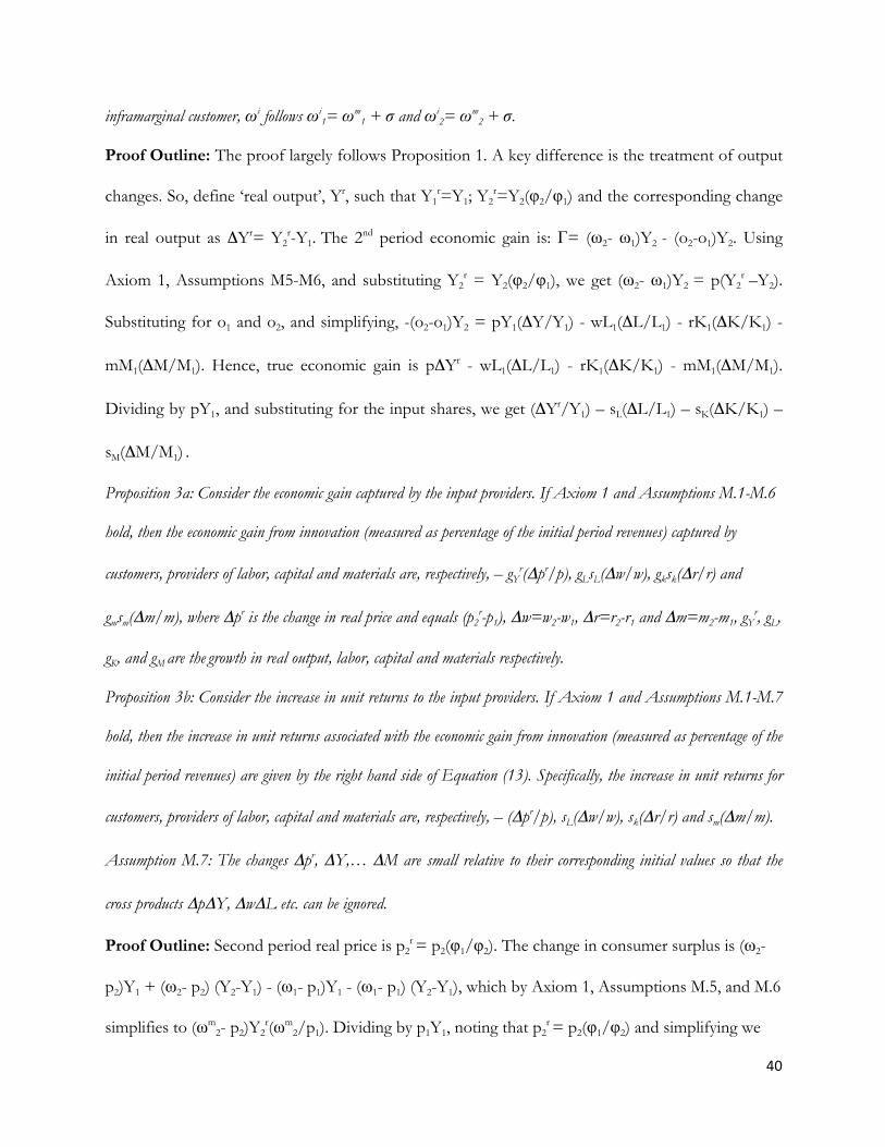
40

inframarginal customer, ωi, follows ωi

1= ωm1 + σ and ωi

2= ωm2 + σ.

Proof Outline: The proof largely follows Proposition 1. A key difference is the treatment of output

changes. So, define ‘real output’, Yr, such that Y1r=Y1; Y2

r=Y2(φ2/φ1) and the corresponding change

in real output as ΔYr= Y2r-Y1. The 2nd period economic gain is: Γ= (ω2- ω1)Y2 - (o2-o1)Y2. Using

Axiom 1, Assumptions M5-M6, and substituting Y2r = Y2(φ2/φ1), we get (ω2- ω1)Y2 = p(Y2

r –Y2).

Substituting for o1 and o2, and simplifying, -(o2-o1)Y2 = pY1(ΔY/Y1) - wL1(ΔL/L1) - rK1(ΔK/K1) -

mM1(ΔM/M1). Hence, true economic gain is pΔYr - wL1(ΔL/L1) - rK1(ΔK/K1) - mM1(ΔM/M1).

Dividing by pY1, and substituting for the input shares, we get (ΔYr/Y1) – sL(ΔL/L1) – sK(ΔK/K1) –

sM(ΔM/M1) .

Proposition 3a: Consider the economic gain captured by the input providers. If Axiom 1 and Assumptions M.1-M.6

hold, then the economic gain from innovation (measured as percentage of the initial period revenues) captured by

customers, providers of labor, capital and materials are, respectively, – gYr(Δpr/p), gLsL(Δw/w), gksk(Δr/r) and

gmsm(Δm/m), where Δpr is the change in real price and equals (p2r-p1), Δw=w2-w1, Δr=r2-r1 and Δm=m2-m1, gY

r, gL,

gK, and gM are the growth in real output, labor, capital and materials respectively.

Proposition 3b: Consider the increase in unit returns to the input providers. If Axiom 1 and Assumptions M.1-M.7

hold, then the increase in unit returns associated with the economic gain from innovation (measured as percentage of the

initial period revenues) are given by the right hand side of Equation (13). Specifically, the increase in unit returns for

customers, providers of labor, capital and materials are, respectively, – (Δpr/p), sL(Δw/w), sk(Δr/r) and sm(Δm/m).

Assumption M.7: The changes Δpr, ΔY,… ΔM are small relative to their corresponding initial values so that the

cross products ΔpΔY, ΔwΔL etc. can be ignored.

Proof Outline: Second period real price is p2r = p2(φ1/φ2). The change in consumer surplus is (ω2-

p2)Y1 + (ω2- p2) (Y2-Y1) - (ω1- p1)Y1 - (ω1- p1) (Y2-Y1), which by Axiom 1, Assumptions M.5, and M.6

simplifies to (ωm2- p2)Y2

r(ωm2/p1). Dividing by p1Y1, noting that p2

r = p2(φ1/φ2) and simplifying we

41

get– gYr(Δpr/p1) whereΔpr= (p2

r-p1) and gYr=(Y2

r/Y1). For labor, note that the change in total wages

are (w2- w1)L1 + (w2- w1)(L2-L1), which simplifies to gLsL(Δw/w1) where sL= w1L1/ p1Y1. To prove

Proposition 3b, replace gYr, gL, gK, and gM with 1 in the above expressions.

Proposition 4: Suppose there exists a competitor that pays its input owners their opportunity costs and with the same

WTP as the focal firm. Let Yc, Lc, Kc and Mc be the competitor’s quantities, pc, wc, rc and mc be the prices, and ρ a

scaling factor such that Yc=ρY1, where Y is the output of the focal firm. Let GM= –sLc(ΔLc/Lc) + sKc(ΔKc/Kc) +

sMc(ΔMc/Mc) where ΔZc=(ρZ1- Zc), Z={L, K, M}, and sLc = (wcLc/pcYc), sKc = (rcKc/pcYc), and sMc =

(mcMc/pcYc). Then, (1/ρ)pcYcGM(Y2-Y1)/Y1 is equal to replication gain as defined in Equation (6).

Proof Outline: GM multiplied by (1/ρ)pcYc is (-wcL1 – rcK1 – mcM1) + (1/ρ)(wcLc + rcKc + mcMc),

which simplifies to pcY1 – wcL1 – rcK1 – mcM1, the true economic value created by the focal firm in

the first period. Dividing by Y1 gives the additional economic value created per unit in the first

period by the firm, and multiplying by (Y2-Y1) gives the replication gain.