Total Maximum Daily Loading · establishment of the Total Maximum Daily Load (TMDL) begins. The TMDL process establishes the allowable loadings of pollutants or other quantifiable

Final Nutrient Total Maximum Daily Load

for Orange Lake,

Alachua County, Florida

Xueqing Gao and Douglas Gilbert

Watershed Assessment Section

Florida Department of Environmental Protection

2600 Blair Stone Road, MS 3555

Tallahassee, FL 32399-2400

September 19, 2003

Table of Contents

Table of Contents...................................................................................... i List of Figures............................................................................................ iii List of Tables............................................................................................. iv Acknowledgements................................................................................... v 1. Introduction...............................................................………………….. 1 1.1. Purpose of Report....................................................…………….. 1 1.2. Identification of Water Body.....................................…………….. 1 2. Description of Standards..................................................................... 3 3. Statement of Problem.......................................................................... 4 4. Assessment of Sources......................................................................... 4

4.1 Types of Sources............................................................................ 4 4.2 Estimating Watershed Loadings of TN and TP using WMM............ 5 Strategy to determine loadings and assimilative capacity.................. 5

Breakdown of sub-basins and Landuses....................................... 5 Potential Sources of TN and TP..................................................... 7 Estimating Watershed TN and TP .................................................. 8

4.3 Lake Modeling using Bathtub Model.............................................. 9 Bathtub Model................................................................................. 9 Bathtub Data Requirements .......................................................... 10 Calculation of Trophic State Index.................................................. 11 Error and Variability Analysis.......................................................... 11

4.4 TMDL Scenario Development........................................................ 12 Available Data and Data Use ........................................................ 12

5. Results.................................................................................................. 13 5.1 Data Analysis................................................................................ 13

Historical trend of trophic status of Orange Lake........................ 13 TN and TP Inlet and Outlet Concentrations................................... 20

5.2 Estimating TN and TP sub-basin loadings Using WMM............... 21 Data required for loading estimation.........……………………… 23 Preparing rainfall data for WMM water quantity calibration........... 29 WMM calibration and Simulation of Watershed Loadings............. 30 Loading from Lochloosa Lake....................................................... 46 Atmospheric Loading to the Lake.................................................. 46 Summary of discharge and TN and TP loadings................................ 47

5.3 Establishing Relationship between TN and TP loading to the Lake and In-Lake Concentrations............................................ 49 Data required by Bathtub model........................................................ 49 Calibrating Bathtub Model............................................................. 51 TSI from Model Predictions vs. TSI from Measured Data............. 54 TP loading vs. TSI of Orange lake................................................... 54

i

Natural Background...................................................................... 56 6. Orange Lake TMDL........................................................................... 58

6.1 Load Allocation............................................................................... 59 6.2 Wasteload Allocation...................................................................... 60 6.3 Margin of Safety............................................................................ 60

7. Next Step............................................................................................... 60 References............................................................................................... 62 Appendix A ................................................................................................ 64

ii

List of Figures

Figure 1 General Location of Watershed.................................................. 2 Figure 2 Orange Lake Sub-basins......................................................... 6 Figure 3 Bathtub Conceptual Scheme...................................................... 9 Figure 4 Location of Data Stations........................................................... 14 Figure 5-A Lake TN Concentration vs. Volume........................................ 18 Figure 5-B Lake TP Concentration vs. Volume........................................ 18 Figure 5-C Lake Chla Concentration vs. Volume..................................... 19 Figure 5-D Lake TSI vs. Volume.............................................................. 19 Figure 6 USGS Gauging Stations and sub-basin delineation’s................ 22 Figure 7 Location of Weather Station....................................................... 24 Figure 8 TN Loading Camp Canal/Styx River OL subbasin.................... 32 Figure 9 TP Loading Camp Canal/Styx River OL subbasin.................... 32 Figure 10 TN Load and Flow from Camp Canal..................................... 33 Figure 11 TP Load and Flow from Camp Canal..................................... 33 Figure 12 Percent TN Loading from Newnans Lake and Camp Canal.. 34 Figure 13 Percent TP Loading from Newnans Lake and Camp Canal.. 34 Figure 14 Percent TN by Landuse 1997................................................ 41 Figure 15 Percent TN by Landuse 2000................................................ 42 Figure 16 Percent TP by Landuse 1997................................................ 43 Figure 17 Percent TP by Landuse 2000................................................ 44 Figure 18 TSI vs. TP Load Reductions.................................................. 55

iii

List of Tables

Table 1 Lake Basin Landuse and acreage................................................ 7 Table 2 Data Types and Period of Record................................................ 12 Table 3 Annual Average Lake TN, TP, Chla, and TSI............................... 15 Table 4 Seasonal Variation of Lake TN, TP, Chla, and TSI...................... 15 Table 5 Lake Annual Average Stage and Volume..................................... 16 Table 6 Lake Quarterly Average Stage and Volume................................. 17 Table 7 Lake Inlet and Outlet Annual Average TN Concentrations........... 20 Table 8 Lake Inlet and Outlet Annual Average TP Concentrations........... 21 Table 9 Annual Precipitation..................................................................... 23 Table 10 Sub-basin Landuses and area................................................... 25 Table 11 Percent Directly Connected Impervious Area by Landuse ........ 26 Table 12 TN and TP Landuse based Event Mean Concentration............. 27 Table 13 Percent suspended TN and TP by Landuse and Sub-basin...... 27 Table 14 Camp Canal Daily discharge, TN and TP Concentration.......... 28 Table 15 Adjusted Effective Rainfall......................................................... 30 Table 16 Simulated Flow and Runoff to the Lake..................................... 30 Table 17 TN and TP Loading to the Lake................................................. 31 Table 18 TN Loads by Landuse and Subbasin (1995 – 2000)................. 35 Table 19 TP Loads by Landuse and Subbasin (1995-2000).................... 37 Table 20 TN and TP Loadings from Lochloosa Lake.............................. 46 Table 21 TN and TP Atmospheric Loadings to Lake............................... 47 Table 22 Sources of Water to the Lake................................................... 47 Table 23 Sources of TN Loading to the Lake.......................................... 47 Table 24 Sources of TP Loading to the Lake......................................... 48 Table 25 Physical Characteristics of Orange Lake by Year.................. 49 Table 26 Precipitation and Evaporation by Year...................................... 50 Table 27 Measured TN, TP, Chla Concentrations of Lake by Year......... 50 Table 28 Flow, TN, and TP Concentrations by Landuse.......................... 50 Table 29 Bathtub Calibration Results ....................................................... 53 Table 30 TSI Measured vs. Predicted....................................................... 54 Table 31 TP Sources to Orange Lake....................................................... 56 Table 32 TP comparision to other studies................................................. 58 Table 33 TMDL Components.................................................................... 59

iv

Acknowledgments

This study could not have been accomplished without the significant contributions from staff within the Watershed Assessment Section. Particular appreciation to Barbara Donner for her contributions. All of the basin delineation’s, landuse aggregations, and much of the data gathering are a result of her efforts. Additional appreciation to Dr. TS Wu for his assistance and insights on modeling and to Dr. Paul Lee for his assistance in understanding the groundwater system. The Department also recognizes the substantial support and assistance provided by the St. Johns River Water Management District staff, particularly their contributions towards understanding the issues, history, and processes at work in the Orange Lake watershed.

v

1. INTRODUCTION 1.1 Purpose of Report This report represents the efforts to develop a nutrient TMDL for Orange Lake (Lake). The Lake, located in Central Florida near Gainesville (Figure 1), was verified as impaired by nutrients based on elevated levels of the Trophic State Index for lakes, and was included on the verified list of impaired waters for the Ocklawaha Basin that was adopted by Secretarial Order on August 26, 2002. According to Section 303(d) of the federal Clean Water Act (CWA) and the Florida Watershed Restoration Act, Chapter 403, Florida Statutes, the Florida Department of Environmental Protection (DEP) is required to submit on a recurring basis lists of surface waters that do not meet applicable water quality standards (impaired waters). The methodologies used by the state for the determination of impairment are established in Rule 62-303, Identification of Impaired waters (IWR), Florida Administrative Code (FAC). Once a water body or water body segment has been verified as impaired and referenced in the Secretarial Order Adopting the Verified List of Impaired Waters, work on establishment of the Total Maximum Daily Load (TMDL) begins. The TMDL process establishes the allowable loadings of pollutants or other quantifiable parameters for a waterbody based on the relationship between pollution sources and in-stream water quality conditions, so that states can establish water quality based controls to reduce pollution from both point and nonpoint sources and restore and maintain the quality of their water resources (USEPA, 1999) 1.2 Identification of Water Body Orange Lake is located in a topographical region of the state that is known as the Central Lowlands (Clark et al. 1964, Latitude 29028’03”, Longitude 82010’58”, Figure 1). The geology of the area is dominated by the Hawthorn formation, which is about 50 feet thick where Orange Lake is located (Scott 1988a). The Hawthorn formation is relatively impermeable and acts as a confining layer to separate the surface water from the influence of the Floridian Aquifer. However, a connection between the lake water and Floridian Aquifer exists through a sink hole system located in the southwest part of Orange Lake. Because the potentiometric surface of this area is about the same as or lower than the long-term average elevation of the lake surface (57.8 feet, Lasi 1999), the movement of the lake water is downward. Therefore, it is not anticipated that the Floridan Aquifer will have a significant direct influence on the lake water quality. The surface area of Orange Lake ranges from 5,000 to 14,7000 acres, depending on the amount of rainfall. The maximum depth of the lake under average conditions is about 12 feet and the mean depth is approximately 5.5 feet (Deevey 1989). Major sources of water to the lake include: (1) interflow via Camps Canal-River Styx from Newnans Lake and Cross Creek from Lochloosa Lake; (2) surface runoff from the watershed; and (3) the direct precipitation into the lake. Water flows out of the lake through the sink hole system located in the southwest part of the lake and through the outlet stream, Orange Creek (Figure 1).

1

For assessment purposes, the State of Florida has been divided into waterbody assessment polygons termed Waterbody Ids or WBIDs. Additional information about derivation and use of these WBIDs is provided in the “Documentation For the 2002 Update to the State Of Florida’s 303(d) List” dated October 1, 2002, and GIS shapefiles of the WBIDs can be obtained from the following website: http://www.floridadep.org/water/watersheds/basin411/downloads.htm

Figure 1. The general location and landuse types of the Orange Lake watershed

2

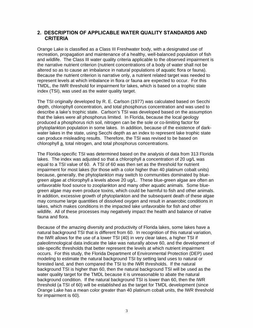
http://www.floridadep.org/water/watersheds/basin411/downloads.htm

2. DESCRIPTION OF APPLICABLE WATER QUALITY STANDARDS AND CRITERIA

Orange Lake is classified as a Class III Freshwater body, with a designated use of recreation, propagation and maintenance of a healthy, well-balanced population of fish and wildlife. The Class III water quality criteria applicable to the observed impairment is the narrative nutrient criterion (nutrient concentrations of a body of water shall not be altered so as to cause an imbalance in natural populations of aquatic flora or fauna). Because the nutrient criterion is narrative only, a nutrient related target was needed to represent levels at which imbalance in flora or fauna are expected to occur. For this TMDL, the IWR threshold for impairment for lakes, which is based on a trophic state index (TSI), was used as the water quality target. The TSI originally developed by R. E. Carlson (1977) was calculated based on Secchi depth, chlorophyll concentration, and total phosphorus concentration and was used to describe a lake’s trophic state. Carlson’s TSI was developed based on the assumption that the lakes were all phosphorus limited. In Florida, because the local geology produced a phosphorus rich soil, nitrogen can be the sole or co-limiting factor for phytoplankton population in some lakes. In addition, because of the existence of dark-water lakes in the state, using Secchi depth as an index to represent lake trophic state can produce misleading results. Therefore, the TSI was revised to be based on chlorophyll a, total nitrogen, and total phosphorus concentrations. The Florida-specific TSI was determined based on the analysis of data from 313 Florida lakes. The index was adjusted so that a chlorophyll a concentration of 20 ug/L was equal to a TSI value of 60. A TSI of 60 was then set as the threshold for nutrient impairment for most lakes (for those with a color higher than 40 platinum cobalt units) because, generally, the phytoplankton may switch to communities dominated by blue-green algae at chlorophyll a levels above 20 ug/L. These blue-green algae are often an unfavorable food source to zooplankton and many other aquatic animals. Some blue-green algae may even produce toxins, which could be harmful to fish and other animals. In addition, excessive growth of phytoplankton and the subsequent death of these algae may consume large quantities of dissolved oxygen and result in anaerobic conditions in lakes, which makes conditions in the impacted lake unfavorable for fish and other wildlife. All of these processes may negatively impact the health and balance of native fauna and flora. Because of the amazing diversity and productivity of Florida lakes, some lakes have a natural background TSI that is different from 60. In recognition of this natural variation, the IWR allows for the use of a lower TSI (40) in very clear lakes, a higher TSI if paleolimnological data indicate the lake was naturally above 60, and the development of site-specific thresholds that better represent the levels at which nutrient impairment occurs. For this study, the Florida Department of Environmental Protection (DEP) used modeling to estimate the natural background TSI by setting land uses to natural or forested land, and then compared the TSI to the IWR thresholds. If the natural background TSI is higher than 60, then the natural background TSI will be used as the water quality target for the TMDL because it is unreasonable to abate the natural background condition. If the natural background TSI is lower than 60, then the IWR threshold (a TSI of 60) will be established as the target for TMDL development (since Orange Lake has a mean color greater than 40 platinum cobalt units, the IWR threshold for impairment is 60).

3

3. STATEMENT OF PROBLEM As noted previously, the IWR threshold for nutrient impairment is an annual TSI of greater than 60. As shown in Table 3, several years of the verified period had annual TSI values greater than 60. In fact, based on summaries of the data contained in the DEP IWR Water Run 9.1 database (IWR-data), the long-term TSI (1989 – 2000) calculated from these data according to the procedures adopted in the IWR is 69, indicating that the high TSIs were not an anomalous event. This long-term TSI was based on long-term average concentrations of total phosphorus (TP), total nitrogen (TN), and chlorophyll a (Chla) were 46 ± 6, 1700 ± 211, and 43.8 ± 9.5 µg/L, respectively (Table 3). While the verified period for listing purposes is June, 1995 – December 2000, this report uses the period from January, 1995 through December, 2000 due to use of annual average values and because no data are available after 2000 in the IWR-database. For the verified period in this report, the TP, TN, and Chla concentrations were 53 ± 9, 1772 ± 363, and 59.2 ± 15.3 ug/L, respectively, and the TSI of the verified period was 73. 4. ASSESSMENT OF SOURCES 4.1 Types of Sources An important part of the TMDL analysis is the identification of source categories, source subcategories, or individual sources of nutrients in the Orange Lake watershed and the amount of pollutant loading contributed by each of these sources. Sources are broadly classified as either “point sources” or “nonpoint sources.” Historically, the term point sources has meant discharges to surface waters that typically have a continuous flow via a discernable, confined, and discrete conveyance, such as a pipe. Domestic and industrial wastewater treatment facilities (WWTFs) are examples of traditional point sources. In contrast, the term “nonpoint sources” was used to describe intermittent, rainfall driven, diffuse sources of pollution associated with everyday human activities, including runoff from urban land uses, runoff from agriculture, runoff from silviculture, runoff from mining, discharges from failing septic systems, and atmospheric deposition. However, the 1987 amendments to the Clean Water Act redefined certain nonpoint sources of pollution as point sources subject to regulation under EPA’s National Pollutant Discharge Elimination Program (NPDES). These nonpoint sources included certain urban stormwater discharges, including those from local government master drainage systems, construction sites over five acres, and from a wide variety of industries (see Appendix A for background information about the State and Federal Stormwater Programs). To be consistent with Clean Water Act definitions, the term “point source” will be used to describe traditional point sources (such as domestic and industrial wastewater discharges) AND stormwater systems requiring an NPDES stormwater permit when allocating pollutant load reductions required by a TMDL (see Section 6). However, the methodologies used to estimate nonpoint source loads do not distinguish between NPDES stormwater discharges and non-NPDES stormwater discharges, and as such, this source assessment section does not make any distinction between the two types of stormwater.

4

4.2 Estimating TN and TP loadings using WMM Overall Strategy to Determine Loadings and Assimilative Capacity The goal of the nutrient TMDL development for Orange Lake is to identify the maximum allowable TP and TN loadings to the lake so that the lake will meet the water quality standard and maintain its function and designated use as a Class III water. Specifically, the goal is interpreted in this study as a TSI of 60 or the natural background TSI if the natural background is higher than 60. Three steps were taken to achieve this goal.

1. TN and TP loadings from the Orange Lake watershed were estimated using the Watershed Management Model (WMM).

2. Loading estimates from the WMM were entered into the Bathtub eutrophication model to establish the relationship between TN and TP loadings and in-lake TN, TP, and Chla concentrations. The model results for in-lake TN, TP, and Chla were used to calculate TSI-predicted (TSI-P) for several different loading scenarios discussed later.

3. The loadings to the lake were adjusted until the TSI-P calculated from the model results was less than 60. The TN and TP loadings that resulted in a TSI compliant with Section 62-303.450, FAC, were considered the nutrient TMDL for Orange Lake.

Breakdown of Orange Lake watershed and landuse categories The Orange Lake watershed drains an area of about 87,339 acres. For modeling purposes, the watershed was divided into two sub-basins (Figure 2). These sub-basins are Camps Canal – River Styx sub-basin (CCRS – area discharging directly into Camps Canal and River Styx), Orange Lake sub-basin (OL – area discharging directly into Orange Lake).

5

"́

"́

"́

"́

"́Orange Creek

Camps Canal

River Styx

Cross Creek

#

Sink Hole System

Prairie Creek

CCRS

OL

3 0 3 6 Miles

N

Figure 2. Sub-basins of Orange Lake watershed. CCRS and OL represent Camps Canal and River Styx sub-basin and Orange Lake sub-basins, respectively. Landuse categories in Orange Lake watershed were aggregated using the simplified level 1 codes tabulated in Table 1. The spatial distribution of different landuse types of Orange Lake watershed is demonstrated in Figure 1.

6

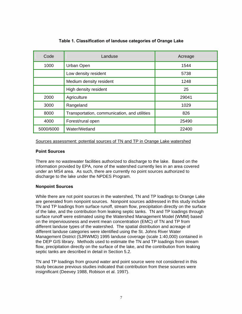
Table 1. Classification of landuse categories of Orange Lake

Code Landuse Acreage

1000 Urban Open 1544

Low density resident 5738

Medium density resident 1248

High density resident 25

2000 Agriculture 29041

3000 Rangeland 1029

8000 Transportation, communication, and utilities 826

4000 Forest/rural open 25490

5000/6000 Water/Wetland 22400 Sources assessment: potential sources of TN and TP in Orange Lake watershed Point Sources There are no wastewater facilities authorized to discharge to the lake. Based on the information provided by EPA, none of the watershed currently lies in an area covered under an MS4 area. As such, there are currently no point sources authorized to discharge to the lake under the NPDES Program. Nonpoint Sources While there are not point sources in the watershed, TN and TP loadings to Orange Lake are generated from nonpoint sources. Nonpoint sources addressed in this study include TN and TP loadings from surface runoff, stream flow, precipitation directly on the surface of the lake, and the contribution from leaking septic tanks. TN and TP loadings through surface runoff were estimated using the Watershed Management Model (WMM) based on the imperviousness and event mean concentration (EMC) of TN and TP from different landuse types of the watershed. The spatial distribution and acreage of different landuse categories were identified using the St. Johns River Water Management District (SJRWMD) 1995 landuse coverage (scale 1:40,000) contained in the DEP GIS library. Methods used to estimate the TN and TP loadings from stream flow, precipitation directly on the surface of the lake, and the contribution from leaking septic tanks are described in detail in Section 5.2. TN and TP loadings from ground water and point source were not considered in this study because previous studies indicated that contribution from these sources were insignificant (Deevey 1988, Robison et al. 1997).

7

Estimating TN and TP loading from Orange Lake watershed using WMM WMM development was originally funded by DEP under contract to Camp Dresser and McKee (CDM). CDM further refined and developed the model to its present state. WMM is a watershed model designed to estimate annual or seasonal pollutant loadings from a given watershed and evaluate the effect of watershed management strategies on water quality (WMM User’s Manual: 1998). While the strength of the model is its capability to characterize pollutant loadings from nonpoint sources, such as those through stormwater runoff, stream baseflow, and leakage of septic tanks, the model handles point sources such as discharge from wastewater treatment facilities and combined sewer overflows (CSOs) as well. Estimation of pollution load reduction due to partial or full-scale implementation of on-site or regional best management practices (BMP) is also part of the functions of this model. The fundamental assumption of the model is that the stormwater runoff from any given landuse is in direct proportion to annual rainfall and is dictated by the portion of the landuse category that is impervious and the runoff coefficients of both pervious and impervious area. The governing equation is:

(1) RL = [Cp + (CI – Cp) IMPL] * I Where:

RL = total average annual surface runoff from land use L (in/yr); IMPL = fractional imperviousness of land use L; I = long-term average annual precipitation (in/yr); CP = pervious area runoff coefficient; and CI = impervious area runoff coefficient.

The model estimates pollutant loadings based on nonpoint pollution loading factors (expressed as lbs/ac/yr) that vary by land use and the percent imperviousness associated with each land use. The pollution loading factor ML is computed for each land use L by the following equation:

(2) ML = EMCL * RL * K Where:

ML = loading factor for land use L (lbs/ac/yr); EMCL = event mean concentration of runoff from land use L (mg/L); EMC

varies by land use and pollutant; RL = total average annual surface runoff from land use L computed

from Equation (1) (in/yr); and K = 0.2266, a unit conversion constant.

Data required for WMM application include:

• Area of all the landuse categories and the area served by septic tanks • Percent impervious area of each landuse category • EMC for each pollutant type and landuse category • Percent EMC of each pollutant type that is in suspended form • Annual precipitation

8

Calibration of WMM is usually conducted on both runoff quantity and quality. This is a two-step procedure since the water quality calibration is a function of the predicted runoff volumes. Calibration of water quantity is usually achieved through adjusting the pervious and impervious area runoff coefficients. Typical ranges of runoff coefficients are 0.05 – 0.30 for pervious area (WMM User’s Manual: 1998) and 0.85 – 1.0 for impervious area (Linsley and Franziani, 1979). After the water quantity calibration, water quality is calibrated by adjusting the pollutant delivery ratio, i.e., the percent quantity of pollutant in the surface runoff that is eventually delivered to the destination waterbody. In this study, the range of the pollutant delivery ratio was estimated using the method developed by Roehl (1962) that correlates the delivery ratio to watershed area. 4.3 Establishing the relationship between TN and TP loading and in-lake TN, TP,

and Chla concentrations using the Bathtub model Bathtub eutrophication model The Bathtub eutrophication model is a suite of empirically derived steady state models developed by the U. S. Army Corps of Engineering (ACOE) Waterways Experimental Station. The primary function of these models is to estimate nutrient concentrations and algal biomass resulting from different patterns of nutrient loadings. The procedures for selection of the appropriate model for a particular lake are described in the Users Manual. The empirical prediction of lake eutrophication using this approach typically can be described as a two-stage procedure using the following two categories of models (Walker 1999):

• Nutrient balance model. This type of model relates in-lake nutrient concentration to external nutrient loadings, morphometry, and hydrology.

• Eutrophication response model. This type of model describes relationships among eutrophication indicators within the lake, including nutrient levels, Chla, transparency, and hypolimnetic oxygen depletion.

Figure 3 describes the concept scheme used by Bathtub to relate external loading of nutrients to the in-lake nutrient concentrations and the physical, chemical, and biological response of the lake to the level of nutrients.

Figure 3. Bathtub concept scheme

Loading of nutrients (Flow and Concentration)

Physical characters of the lake In-lake nutrient Chla, Secchi (Surface area and mean depth) Concentrations (TN&TP) DO

Hydraulic characters of the lake (Water residence time)

The nutrient balance model adopted by Bathtub assumes that the net accumulation of nutrients in a lake is the difference between nutrient loadings into the lake from various

9

sources and the nutrients carried out through outflow and losses of nutrient through whatever decay process occur inside lake:

(3) Net accumulation = Inflow – Outflow – Decay In this study, “inflow” included TN and TP loadings from the interflow of inlet streams (Camps Canal and Cross Creek), stormwater surface runoff from various landuse categories, leakage of septic tanks, and direct atmosphere precipitation into the lake. Nutrient outflow was primarily through the seepage of the sink hole system and the outflow stream: Orange Creek. To address nutrient decay within the lake, Bathtub provided several alternative mass balance models depending on the inorganic/organic nutrient partitioning coefficient and reaction kinetics. The major pathway of decay for TN and TP in the model is through sedimentation to the bottom of the lake.

Prediction of the eutrophication response by Bathtub also involves choosing through several alternative models depending on whether the algal communities are limited by phosphorus or nitrogen, or co-limited by both nutrients. Scenarios that include algal communities limited by light intensity or controlled by the lake flushing rate are also included in the suit of models. In addition, the response of chlorophyll a concentration to the in-lake nutrient level is characterized by two different kinetic processes: linear or exponential. The variety of models available in Bathtub allows the users to choose specific models based on the particular condition of the project lake.

One feature offered by Bathtub is the “calibration factor.” The empirical models implemented in Bathtub are mathematical generalizations about lake behavior. When applied to data from a particular reservoir, measured data may differ from predictions by a factor of two or more. Such differences reflect data limitations (measurement or estimation errors in the average inflow and outflow concentrations), unique features of the particular lake (Walker 1999), and unexpected processes inherent to the lake. The calibration factor offered by Bathtub provides model users with a tool to calibrate the magnitude of lake response predicted by the empirical models. The model calibrated to current conditions against measured data from the lake can then be applied to predict changes in lake conditions likely to result from specific management scenarios under the condition that the calibration factor remains constant for all prediction scenarios. Data requirements for running Bathtub Data requirements for Bathtub model include:

• Physical characteristics of the lake (surface area, mean depth, length, and mixed layer depth)

• Meteorological data (precipitation and evaporation) • Measured water quality data (TN, TP, and Chla concentrations of the lake water,

TN and TP concentrations in precipitation, etc.) • Loading data (flow and TN and TP concentrations of the flow from various

landuse categories, inlet streams, outlet streams, and the TN and TP contribution from the leakage of septic tanks)

• Coefficient of variance (CV) of all the measured data

10

Calculation of Trophic State Index (TSI) TSI was calculated using the procedures outlined in Florida’s 1996 305(b) report:

CHLATSI = 16.8 + 14.4 × LN (CHLA)] TNTSI = 56 + [19.8 × LN (TN)] TN2TSI = 10 × [5.96 + 2.15 × LN (TN + 0.0001)] TPTSI = [18.6 × LN (TP × 1000)] –18.4 TP2TS = 10 × [2.36 × LN (TP × 1000) – 2.38]

Limiting nutrient considerations for calculating NUTRTSI: If TN/TP > 30 then NUTRTSI = TP2TSIIf TN/TP < 10 then NUTRTSI = TN2TSI If 10 < TN/TP < 30 then NUTRTSI = (TPTSI + TNTSI)/2 TSI = (CHLATSI + NUTRTSI)/2

Error and variability analysis The distinction between “error” and “variability” is important. Error refers to a difference between a measured and a predicted mean value and is usually described as: The absolute value of |measurement – prediction|/measurement. Variability refers to spatial or temporal fluctuations in measurement around the mean. Spatial variability is not usually included in the variability analysis of empirical modeling efforts. Empirical modeling variability analysis usually concentrates on those changes caused by temporal fluctuation. Variability is frequently described using the mean coefficient of variance (CV), which is defined as the standard error (SE) of the estimate expressed as a fraction of the predicted value (Walker 1999). In this study, model estimates were presented as mean ± 1SE whenever a CV could be determined. When WMM was used to simulate TN and TP loadings from surface runoff, neither error analysis nor variability analysis were conducted. This was because no flow data were available from any gauging station located within the Orange Lake watershed. In addition, the variability analysis within WMM required CVs for the EMC of TN and TP from different landuse categories and the CV for the suspended fraction of TN and TP from different landuse categories. Because we did not have these CVs, the variability analysis was not conducted using WMM. WMM simulation was conducted for all the years for which there were data. Model predictions for all the years were later averaged to calculate the long-term annual mean and CV, which are required for the error and variability analysis for Bathtub. Bathtub allows the input of the CV for both measured data and model predictions from WMM. Therefore, both error and variability analyses were conducted with Bathtub. To accomplish this, several years of measured data from the non-model variables (precipitation, lake volume, and evaporation) and the WMM predictions (TN, TP, and flow) were averaged and the mean values and CVs of these data were entered to Bathtub as input.

11

4.4 TMDL development for Orange Lake Once WMM and Bathtub model calibrations were achieved, TMDL of the lake was developed through evaluating TSIs of the following scenarios: A. TSI of current condition B. TSI after the loadings from all human landuse categories (urban open, low, medium,

and high density residential, agriculture and rangeland, and transportation, communication, and utilities) within the watershed were assessed as the landuse category Forest/Rural Open. This is the watershed Natural Background condition

C. TSI after all the loadings from human landuse categories were assessed as natural background and the TN and TP loadings from the two upper reach lakes, i.e. Newnans Lake and Lochloosa Lake, through the interflow of Camps Canal-River Styx and Cross Creek achieved their TMDL goals.

The scenario C was considered the natural background condition of the lake. If the TSI of scenario C was lower than 60, the loadings from human landuse would be allowed to increase and up to the final TSI of 60. If the TSI of Scenario C were higher than 60, then the Natural Background TSI would become the target for the TSI. Requirement for historical data, overall data availability and the years from which data were chosen for the modeling Model calibration and simulation of this study requires that several types of data should have measured historical record. These data types and their availability are listed in Table 2. Table 2. Data types that are required to have historical records and the period these data are availability

Data type Available time period

Precipitation 1995 – 2000

Stream flow at the mouth of Camps Canal 1990 –2000

Lake stage 1989 –2000

Stream water quality data 1995 – 2000

Lake water quality data 1989 –2000 Because calibration of the model requires that data from the different types be in the same time period, 1995 to 2000 were chosen as the years from which data were used for model calibration.

12

5. RESULTS

5.1 Data Analysis Historical trend of trophic status of Orange Lake Monthly TN, TP, and Chla concentrations for Orange Lake from 1989 through 2000 were retrieved from the IWR database. The locations of the individual stations from which water quality data were collected are shown in Figure 4. Analysis of the data indicated that the spatial variation between stations across Orange Lake is not significant. Therefore, data from all the stations within the lake were pooled together and treated as data collected from one station. Quarterly mean values for TN, TP, and Chla concentrations were calculated based on the monthly data. Quarterly TSIs were calculated based on the quarterly mean values of TN, TP, and Chla concentrations, and quarterly TN, TP, Chla, and TSI values were then used to calculate annual mean values. The long term annual average values of these data were calculated based on annual mean values of each year from 1989 through 2000. The individual annual average values for the verified period were calculated based on the mean values from 1995 through 2000. The seasonal trend of TN, TP, Chla, and TSI were examined by calculating the long-term quarterly mean values based on the quarterly mean values of each year (1989 – 2000). The quarterly means for the verified period were calculated using the data from 1995 through 2000. The individual annual mean TN, TP, Chla, and TSI values are listed in Table 3 and the long-term quarterly TN, TP, Chla, and TSI results are listed in Table 4.

13

#

#

# #

#

#

#

#

#

#

#

Orange Creek

Camps Canal

River Styx

Cross Creek

#

Sink Hole System

Prairie Creek

CCRS

OL

3 0 3 6 Miles

N

Figure 4. Locations of water quality stations

14

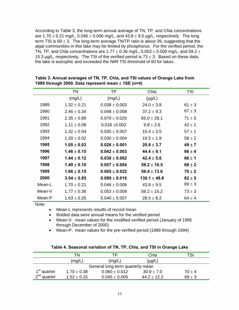
According to Table 3, the long-term annual average of TN, TP, and Chla concentrations are 1.70 ± 0.21 mg/L, 0.046 ± 0.006 mg/L, and 43.8 ± 9.5 µg/L, respectively. The long term TSI is 69 ± 3. The long-term average TN/TP ratio is about 39, suggesting that the algal communities in this lake may be limited by phosphorus. For the verified period, the TN, TP, and Chla concentrations are 1.77 ± 0.36 mg/L, 0.053 ± 0.009 mg/L, and 59.2 ± 15.3 µg/L, respectively. The TSI of the verified period is 73 ± 3. Based on these data, the lake is eutrophic and exceeded the IWR TSI threshold of 60 for lakes.

Table 3. Annual averages of TN, TP, Chla, and TSI values of Orange Lake from 1989 through 2000. Data represent mean ± 1SE (n=4)

TN TP Chla TSI (mg/L) (mg/L) (µg/L)

1989 1.32 ± 0.21 0.038 ± 0.003 24.0 ± 3.8 61 ± 3 1990 2.46 ± 0.34 0.048 ± 0.008 37.2 ± 9.3 67 ± 3

1991 2.35 ± 0.89 0.070 ± 0.020 65.0 ± 28.1 71 ± 5 1992 1.11 ± 0.08 0.018 ±0.002 9.8 ± 2.6 43 ± 1 1993 1.32 ± 0.04 0.035 ± 0.007 15.4 ± 3.5 57 ± 1 1994 1.20 ± 0.02 0.030 ± 0.004 19.5 ± 1.9 58 ± 2 1995 1.05 ± 0.03 0.026 ± 0.001 20.6 ± 3.7 49 ± 7 1996 1.46 ± 0.15 0.042 ± 0.003 44.4 ± 9.1 66 ± 4 1997 1.44 ± 0.12 0.038 ± 0.002 42.4 ± 5.6 66 ± 1 1998 1.49 ± 0.10 0.057 ± 0.004 59.2 ± 10.5 68 ± 2 1999 1.66 ± 0.15 0.065 ± 0.022 58.4 ± 13.6 70 ± 2 2000 3.54 ± 0.85 0.089 ± 0.016 130.1 ± 48.8 82 ± 5

Mean-L 1.70 ± 0.21 0.046 ± 0.006 43.8 ± 9.5 69 ± 3

Mean-V 1.77 ± 0.36 0.053 ± 0.009 59.2 ± 15.2 73 ± 3 Mean-P 1.63 ± 0.25 0.040 ± 0.007 28.5 ± 8.2 64 ± 4

Note: • Mean-L represents results of record mean • Bolded data were annual means for the verified period. • Mean-V: mean values for the modified verified period (January of 1995

through December of 2000) • Mean-P: mean values for the pre-verified period (1989 through 1994)

Table 4. Seasonal variation of TN, TP, Chla, and TSI in Orange Lake

TN TP Chla TSI (mg/L) (mg/L) (µg/L)

General long-term quarterly mean 1st quarter 1.70 ± 0.38 0.060 ± 0.012 30.9 ± 7.0 70 ± 4 2nd quarter 1.52 ± 0.15 0.045 ± 0.005 44.2 ± 12.2 69 ± 3

15

3rd quarter 1.80 ± 0.35 0.043 ± 0.008 54.3 ± 20.9 70 ± 4 4th quarter 1.89 ± 0.40 0.045 ± 0.008 46.0 ± 15.4 69 ± 4

Quarterly mean for the verified period 1st quarter 1.35 ± 0.11 0.056 ± 0.015 34.5 ± 5.9 69 ± 4 2nd quarter 1.64 ± 0.21 0.049 ±0.006 50.4 ± 11.4 71 ± 4 3rd quarter 1.98 ± 0.55 0.053 ± 0.013 84.6 ± 32.4 75 ± 5 4th quarter 2.12 ± 0.65 0.053 ± 0.013 67.3 ± 23.8 74 ± 4 Data represent mean ±1SE. n equals to 12 years for the general long-term quarterly mean values and 6 for quarterly mean values for the verified period. There was a sudden increase and subsequent decrease of TN, TP, and Chla concentrations between 1989 and 1992. During the period from 1992 through 2000, a continuous increase of TN, TP, and Chla concentrations was observed. TN, TP, and Chla increased by 218% (from 1.11 mg/L in 1992 to 3.54 mg/L in 2000), 407% (from 0.018 mg/L in 1992 to 0.089 mg/L in 2000), and 1224% (from 9.8 µg/L in 1992 to 130.1 µg/L in 2000) during this time period, respectively (Table 3). At the same time, TSI increased by 93% from 43 in 1992 to 82 in 2000. Although dramatic changes of annual TN, TP, and Chla concentrations were observed between years, seasonal variation was not very obvious, except that the mean value of Chla concentration of the first quarter was significantly lower than that of the third quarter. The TN, TP, Chla, and TSI values of all the other quarters were not significantly different from each other throughout an average year (Table 4). To explain the annual variation, stage data of Orange Lake collected from 1989 through 2000 were converted to lake volumes using the Elevation – Lake Volume curve of Orange Lake developed by the St. John River Water Management District (Robison 1997). The annual average stage elevation and lake volume are listed in Table 5. The long-term quarterly average stage elevation and lake volume calculated based on data from 1989 through 2000 are listed in Table 6.

Table 5. Annual average stage elevation and volume of Orange Lake. Data represent mean SE (n=4)

Stage elevation Lake volume

(feet) (acre-foot)

1989 56.6 ± 0.4 56750 ± 4888

1990 54.4 ± 0.4 34000 ± 4163

1991 54.1 ± 0.8 33000 ± 7360

1992 54.7 ± 0.4 56 0 ± 0 3

37250 ± 3794

1993 56.0 ± 0.3 50000 ± 2677

1994 56.5 ± 0.3 54450 ± 3853

1995 57.9 ± 0.2 72500 ± 2784

1996 58.3 ± 0.1 77750 ± 946

16

1997 57.6 ± 0.1 68500 ± 1893 1998 58.7 ± 0.4 83250 ± 5329

1999 56.9 ± 0.5 60250 ± 5406

2000 53.1 ± 0.8 25250 ± 5836

Mean 56.3 ± 0.5 54413 ± 4078

Low stage elevation and lake volume for Orange Lake was observed in 1990, 1991, and 2000. This is consistent with the explanation that the high TN, TP, and Chla concentrations of these years might be caused by the concentration process (Table 5). However, lake volume alone obviously can not explain the dynamics of TN, TP, and Chla concentrations in all the other years. According to Figure 5-A, B, C, and D, lake volume steadily increased from 1992 through 1998. TN, TP, and Chla concentrations also increased during the same time period and these increases could have been caused by the increase of TN and TP loading into the lake.

Table 6. Quarterly average stage elevation and volume of Orange Lake. Data represent mean SE (n=6).

Stage elevation Lake volume

(feet) (acre-foot)

1st quarter 56.6 ± 0.6 58542 ± 6454

2nd quarter 56.2 ± 0.5 53358 ± 5910

3rd quarter 56.0 ± 0.5 51833 ± 5476

4th quarter 56.3 ± 0.6 55727 ± 5663

17

0.000

0.500

1.000

1.500

2.000

2.500

3.000

3.500

4.000

4.500

5.000

1989 1990 1991 1992 1993 1994 1995 1996 1997 1998 1999 2000Year

TN c

once

ntra

tion

(mg/

L)

0

10000

20000

30000

40000

50000

60000

70000

80000

90000

100000

Lake

Vol

ume

(acr

e-fe

et)

TN

Lake Volume

Figure 5-A TN concentration vs. volume of Orange Lake

0.000

0.020

0.040

0.060

0.080

0.100

0.120

1989 1990 1991 1992 1993 1994 1995 1996 1997 1998 1999 2000

Year

TP c

once

ntra

tion

(mg/

L)

0

10000

20000

30000

40000

50000

60000

70000

80000

90000

100000

Lake

Vol

ume

(acr

e-fe

et)

TP

Lake Volume

Figure 5-B. TP concentration vs. volume of Orange Lake

18

0.000

20.000

40.000

60.000

80.000

100.000

120.000

140.000

160.000

180.000

200.000

198919901991 199219931994 199519961997 199819992000

Year

Chl

a co

ncen

trat

ion

(µg/

L)

0

10000

20000

30000

40000

50000

60000

70000

80000

90000

100000

Lake

Vol

ume

(acr

e-fe

et)

Chla

Lake Volume

Figure 5-C. Chla concentration vs. volume of Orange Lake

0.000

10.000

20.000

30.000

40.000

50.000

60.000

70.000

80.000

90.000

100.000

1989 1990 1991 1992 1993 1994 1995 1996 1997 1998 1999 2000

Year

TSI

0

10000

20000

30000

40000

50000

60000

70000

80000

90000

100000

Lake

Vol

ume

(acr

e-fe

et)

TSI

Lake Volume

Figure 5-D. TSI vs. lake volume of Orange Lake

19

No clear long-term seasonal trend was found with the lake volume (Table 6). This was consistent with the findings that TN, TP, Chla, and TSI did not show significant variation between different quarters of an average year. TN and TP concentrations of inlet and outlet streams and the sink hole system of Orange Lake Orange Lake has two major inlet streams including the Camps Canal – River Styx and Cross Creek. Measured TN and TP concentrations were only available for Cross Creek. TN and TP concentrations for Camps Canal – River Styx was estimated by dividing the sum of TN and TP loads of the interflow from the Prairie Creek and TN and TP load in the surface runoff from CCRS sub-basin into Camps Canal – River Styx system by the total volume of the interflow and surface run off. TN and TP loads from the surface runoff and the volume of the surface runoff were estimated using WMM as shown in a later section. No directly measured TN and TP concentrations were available for the two major outlets (the Orange Creek and the sink hole system). For modeling purpose, TN and TP concentrations of these outlets were considered equal to the lake concentrations. TN and TP concentrations for the major inlets and outlets of Orange Lake are listed in Table 7 and Table 8, respectively.

Table 7. Annual average TN concentration of Camps Canal – River Styx, Cross Creek, Orange Creek, and the sink hole system. Data represent mean ± SE. Unit: mg/L

Inlets Outlets

Camps Canal-River Styx Cross Creek Orange Creek Sink Hole

System 1989 ---- ---- 1.32 ± 0.21 1.32 ± 0.21

1990 ---- ---- 2.46 ± 0.34 2.46 ± 0.34

1991 ---- ---- 2.35 ± 0.89 2.35 ± 0.89

1992 ---- ---- 1.11 ± 0.08 1.11 ± 0.08

1993 ---- ---- 1.32 ± 0.04 1.32 ± 0.04

1994 ---- ---- 1.20 ± 0.02 1.20 ± 0.02

1995 3.79 1.64 ± 0.44 1.05 ± 0.03 1.05 ± 0.03

1996 3.34 1.87 ± 0.17 1.46 ± 0.15 1.46 ± 0.15

1997 3.14 1.90 ± 0.38 1.44 ± 0.12 1.44 ± 0.12

1998 2.03 1.68 ± 0.10 1.49 ± 0.10 1.49 ± 0.10

1999 2.54 ---- 1.66 ± 0.15 1.66 ± 0.15

2000 0.96 ---- 3.54 ± 0.85 3.54 ± 0.85

Mean 2.70 ± 0.42 1.78 ± 0.10 1.77 ± 0.36 1.77 ± 0.36

20

Table 8. Annual average TP concentration of Camps Canal – River Styx, Cross Creek, Orange Creek, and the sink hole system. Data represent mean ± SE. Unit: mg/L

Inlets Outlets

Camps Canal-River Styx Cross Creek Orange Creek Sink Hole

System 1989 ---- ---- 0.038 ± 0.003 0.038 ± 0.003

1990 ---- ---- 0.048 ± 0.008 0.048 ± 0.008

1991 ---- ---- 0.070 ± 0.020 0.070 ± 0.020

1992 ---- ---- 0.018 ± 0.002 0.018 ±0.002

1993 ---- ---- 0.035 ± 0.007 0.035 ± 0.007

1994 ---- ---- 0.030 ± 0.004 0.030 ± 0.004

1995 0.193 0.055 ± 0.020 0.026 ± 0.001 0.026 ± 0.001

1996 0.128 0.050 ± 0.008 0.042 ± 0.003 0.042 ± 0.003

1997 0.127 0.067 ± 0.009 0.038 ± 0.002 0.038 ± 0.002

1998 0.116 0.078 ± 0.005 0.057 ± 0.004 0.057 ± 0.004

1999 0.171 ---- 0.065 ± 0.022 0.065 ± 0.022

2000 0.096 ---- 0.089 ± 0.016 0.089 ± 0.016

Mean 0.138 ± 0.015 0.062 ± 0.006 0.053 ± 0.009 0.053 ± 0.009 The mean values listed in Table 7 and Table 8 were calculated based on the annual mean values of the years within the verified period (1995 through 2000). TN and TP concentrations of Cross Creek in 1999 and 2000 were unavailable. Therefore, the mean annual TN and TP concentrations of Cross Creek were calculated based on the annual means of 1995 through 1998. It appears that TN and TP concentrations of the two inlet streams were either similar to (Cross Creek) or significantly higher (Camps Canal – River Styx) than TN and TP concentrations of the lake, suggesting that the TN and TP concentrations of Orange Lake were controlled by the external loading of TN and TP. 5.2 Estimating TN and TP loadings from CCRS and OL sub-basins using WMM External loadings of TN and TP from CCRS and OL sub-basins into Orange Lake were estimated using WMM in this study. TN and TP loadings from CCRS sub-basin discharge into Orange Lake primarily through Camps Canal – River Styx. However, surface runoff is not the only source of water discharged through the Camp Canal – River Styx system. Interflow from Prairie Creek conveyed a significant amount of outflow water from Newnans Lake into Orange Lake watershed. To estimate the total loadings of TN and TP through the Camps Canal – River Styx system using WMM, the interflow measured at the USGS gauging station 02241000 (Figure 6) was treated as a point source whose TN and TP concentrations were considered the same as the TN and TP concentrations of Prairie Creek.

21

"́

"́

"́

"́"́ Orange Creek

Camps Canal

River Styx

Cross Creek

#

Sink Hole System

Prairie Creek

CCRS

OL

02241000

02241100

02242401

02242451

02242450

3 0 3 6 Miles

N

Figure 6. Locations of USGS gauging stations in Orange Lake watershed.

22

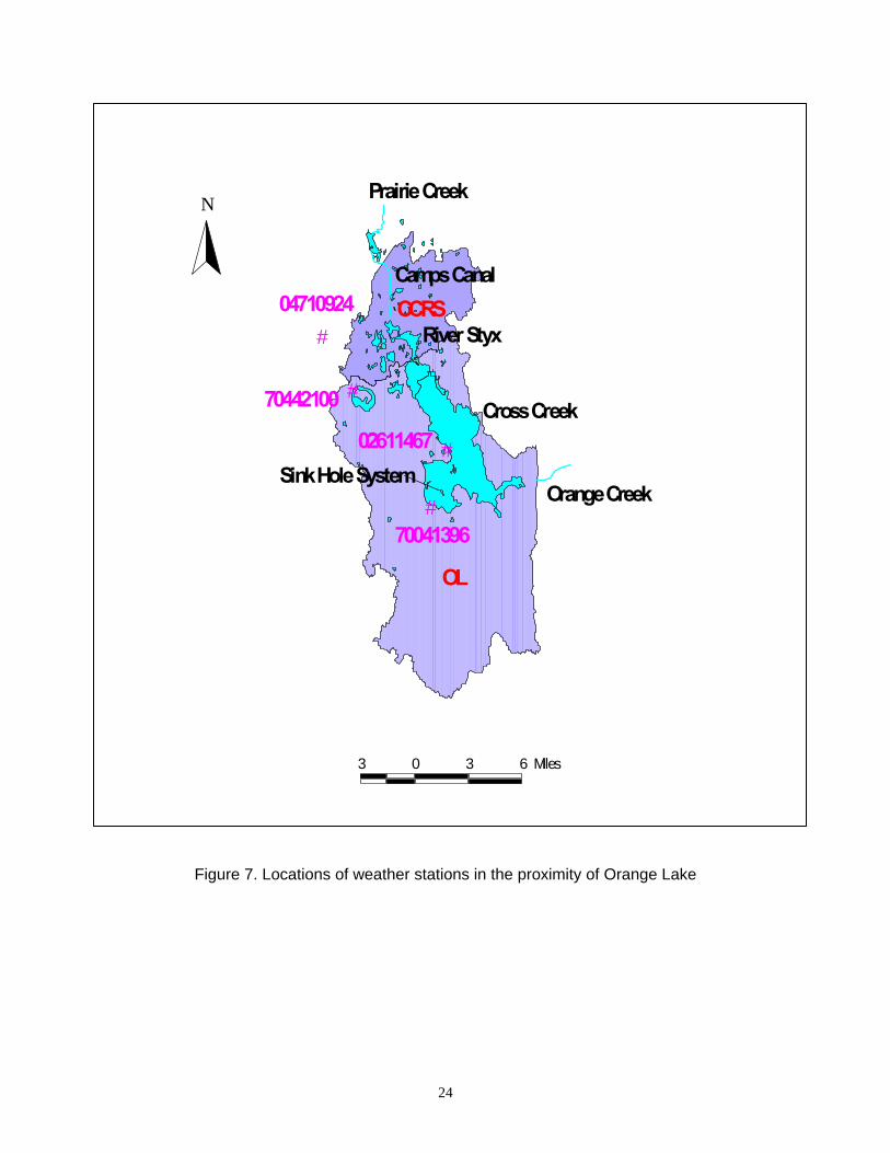
Because no measured flow and TN and TP data were available for the Camps Canal – River Styx system, WMM calibration was not conducted. Most of the model parameters used to estimate the TN and TP loading through surface runoff were borrowed from the TMDL study carried out for the Newnans Lake watershed. These model parameters were also applied when estimating the TN and TP loadings from the OL sub-basins. Data required for estimating TN and TP loadings from CCRS and OL sub-basin using WMM A. Rain precipitation data were collected from four weather stations in the proximity of

Orange Lake (Figure 7). Precipitation data from none of these weather stations covered the entire period from 1995 through 2000. Therefore, precipitation data from all the weather stations were combined and treated as from one composite station. Whenever precipitation data were available at more than one weather station in a given year, composite mean was calculated and used as the precipitation of the year for the composite weather stations. The composite precipitation data are listed in Table 9.

Table 9. Annual precipitation at Gainesville Regional Airport

Year Annual Precipitation (in/year)

1995 49.99 ± 1.06

1996 50.04 ± 1.60

1997 58.92 ± 3.35

1998 46.03 ± 0.23

1999 44.03

2000 33.12

Note: Precipitation data were only available at one weather station in 1999 and 2000.

23

#

#

#

# Orange Creek

Camps Canal

River Styx

Cross Creek

#

Sink Hole System

Prairie Creek

CCRS

OL

70442100

02611467

70041396

04710924

3 0 3 6 Miles

N

Figure 7. Locations of weather stations in the proximity of Orange Lake

24

B. Areas of different landuse categories in each sub-basin were obtained by aggregating GIS landuse coverage based on the simplified level 1 code listed in Table 1. Acreage of each landuse category for CCRS and OL sub-basins is listed in Table 10. Percent distributions of each landuse category in CCRS and OL sub-basins are shown in Figure 8.

Table 10. Area of each landuse category of CCRS and OL sub-basins Unit: acre CCRS OL

Forest/Rural Open 10094 15342

Urban Open 36 1494

Agriculture 1273 27751

Low Density Residential 281 5398

Medium Density Residential 106 1082

High Density Residential 0 13

Communication and Transportation 27 799

Rangeland 211 819

Water/Wetlands 4976 17316

Total 17004 70014

Non-human landuse categories including Water/Wetland and Forest/Rural account for about 85% of the total acreage of CCRS sub-basin (Water/wetland 25% and Forest/rural 60%, Figure 8). The leading human landuse category in CCRS sub-basin is Agriculture, which accounts for 7% of the total acreage. The second largest human landuse category is the Low Density Residential, which accounts for 2% of the total acreage. Landuse categories include Medium Density Residential, Transportation and communication, and Rangeland all account for 1% of the total watershed area. No High Density Residential exists in CCRS sub-basin. The total human landuse accounts for about 12% of the total acreage of the watershed, indicating that the watershed may be relatively undeveloped. Landuse pattern in OL sub-basin is different from CCRS sub-basin. While non-human landuse only accounts for 47% (Water/Wetland 25% and Forest/Rural 22%) of the total acreage, much less than in CCRS, Agricultural claims about 39% of the total watershed area. The second largest human landuse is the Low Density Residential, which accounts for 8% of the watershed. Medium Density Residential ranks the third, about 2% of the total watershed area. Rangeland and Transportation and communication both occupy 1% of the watershed. Again, the High Density Residential is not important in OL sub-basin. The total human landuse claims about 53% of the OL sub-basin, suggesting a significant influence from human activities on the landuse pattern of the watershed. C. Percent impervious area of each landuse category is a very important parameter in

estimating surface runoff using WMM. Non-point pollution monitoring studies

25

throughout the U.S. over the past 15 years have shown that annual “per acre” discharges of urban stormwater pollution are positively related to the amount of imperviousness in the landuse (WMM User’s Manual 1998). Ideally, impervious area is considered as the area that does not retain water and therefore, 100% of the precipitation falling on the impervious area should become surface runoff. In practice, the runoff coefficient for impervious area typically ranges between 95 to 100%. Impervious runoff coefficients lower than this range were observed in the literature, but usually this number should not be lower than 80%. For pervious area, the runoff coefficient usually ranges between 10 to 20%. However, values lower than this range were also observed (WMM User’s Manual: 1998). In this study, 0.95 was used as the runoff coefficient for impervious area and 0.17 was used as the runoff coefficient for pervious area, and is consistent with what was observed with the TMDL study conducted on Newnans Lake.

It should be noted that the impervious area percentages do not necessarily represent directly connected impervious area (DCIA). Using a single-family residence as an example, rain falls on rooftops, sidewalks, and driveways. The sum of these areas may represent 30% of the total lot. However, much of the rain that falls on the roof drains to the grass and infiltrates to the ground or runs off the property and thus does not run directly to the street. For WMM modeling purpose, whenever the area of the watershed that contributes to the surface runoff was considered, DCIA was used in place of impervious area. Because local values were not available, DCIAs used in this study were collected from literature published values or results from other studies (Table 11).

Table 11 Percent direct connected impervious area for different landuse categories

Landuse Categories DCIA Reference

Forest/Rural Open 0.5% WMM User’s Manual: 1998

Urban Open 0.5% WMM User’s Manual: 1998

Agriculture 3.7% Brown 1995

Low Density Residential 12.40% Brown 1995

Medium Density Residential 18.70% Brown 1995

High Density Residential 29.60% Brown 1995

Communication and Transportation 36.20% Brown 1995

Rangeland 3.7% CDM

Water/Wetlands 30% Harper and Livingston 1999

D. Local Event mean concentrations (EMC) of TN and TP for different landuse

categories were not available and therefore were obtained from literature values (Table 12).

26

Table 12. Event mean concentration of TN and TP for different landuse categories Unit: mg/L

Landuse Categories TN TP Reference

Forest/Rural Open 1.25 0.053 Harper 1992

Urban Open 1.59 0.220 Harper 1992

Agriculture 2.58 0.465 Harper 1992

Low Density Residential 1.77 0.177 Harper 1992

Medium Density Residential 2.29 0.300 Harper 1992

High Density Residential 2.42 0.490 Harper 1992

Communication and Transportation 2.08 0.340 Harper 1992

Rangeland 1.25 0.053 Harper 1992

Water/Wetlands 1.60 0.189 Harper 1992

EMCs of TN and TP for most landuse categories were cited from a review prepared by Harper (1992). EMCs for Agriculture, Low Density Residential, and Water/Wetlands were directly provided by the review. However, EMCs for Urban Open, Medium Density Residential, High Density Residential, Transportation and Communication, and Rangeland were not directly defined in Harper’s review. Therefore, some extrapolations were made between the landuse categories in this study and the landuse categories defined by Harper’s review. Basically, the Urban Open area in our study was treated as the Low-Intensity Commercial area in Harper’s review. Medium Density Residential was treated as Single Family area; High Density Residential was treated as Multi-Family area; Transportation and Communication was treated mainly as Highway; and Rangeland was treated the same as Forest/rural.

E. Not all the TN and TP are transported by the stormwater in the dissolved form. The

percentage of the total EMC represented by TN and TP attached to suspended particles is allowed to be defined in WMM. Percent suspended TN and TP values were reported by Lasi (1999) for Orange Lake watershed and were used in this study (Table 13).

Table 13. Percent TP and TN in suspended form for different landuse categories.

Landuse Categories TP TN

Forest/Rural Open 28% 6%

Urban Open 57% 44%

Agriculture 38% 20%

Low Density Residential 57% 44%

Medium Density Residential 57% 44%

27

High Density Residential 57% 44%

Communication and Transportation 57% 44%

Rangeland 38% 20%

Water/Wetlands 48% 77%

F. The sediment delivery ratio determines how much TN and TP attaching to

suspended particles will be delivered to the destination waterbody eventually. In this study, the range of sediment delivery ratio was estimated using the correlation between delivery ratio and watershed area developed by Roehl (1962). Because of the difference in total area of the watershed, CCSR and OL sub-basins were assigned different sediment delivery ratios, which were 0.18 and 0.10, respectively.

G. To estimate the TN and TP loadings from leakage of septic tanks, WMM incorporates the concept of “septic tank failure loading rate” which defines the percent increase of TN and TP loadings. The annual failure rate reported for the country is 3-5 percent. Pollutant loading rates reported in the WMM Users Manual assume 50 gallons per capita per day usage. The mid-range of loading rates for failing septic tanks in the Manual is 2.0 mg/L for TP (about a 160% to 250% increase) and for TN is 15 mg/L (about a 140% to 200% increase). To provide a Margin of Safety, this study adopted the high end of the range in the Users Manual, which were 30 mg/L for TN and 4.0 mg/L for TP (WMM User Manual: 1998). Another value required by WMM to estimate the influence from leaking septic tanks on TN and TP loading is the “septic tank failure rate”, which defines the frequency at which septic tanks may fail. Studies conducted on the water quality of the Ocklawaha River Basin found that annual frequency of septic tank repairs was about 0.97% (Basin Status Report 2001). For average annual conditions, it is conservative to assume that septic tank systems failures would be unnoticed or ignored for fives years before repair or replacement occurred (WMM User Manual: 1998). Therefore, the septic tank failure rate used in this study was calculated by multiplying repairing frequency (0.97%) by 5 (years) and was about 5%.

H. To estimate the TN and TP loading discharged through Camps Canal – River Styx

system into Orange Lake, interflow from Prairie Creek was included in the WMM modeling. To do this, the interflow was treated as a point source and was characterized by the flow data measured at the USGS gauging station 02241000 (Figure 6) and TN and TP concentrations of Prairie Creek. The daily discharge and the TN and TP concentrations of the discharge are listed in Table 14.

Table 14. Daily discharge and TN and TP concentrations in the discharge of Camps Canal at the USGS gauging station 02241000

Daily Discharge TN TP (MGD) (mg/L) (mg/L)

1995 17.48 4.69 0.223 1996 17.63 4.19 0.138 1997 15.09 4.44 0.143 1998 63.91 2.09 0.117

28

1999 3.91 4.74 0.242 2000 0.00 4.03 0.172

Preparing rainfall data for WMM water quantity calibration As it has been discussed in the Method section, WMM uses Equation (1) to estimate the surface runoff from precipitation data. Equation (1) assumes that the amount of surface runoff is in direct proportion to precipitation, which implies that all the rainfall precipitation to some extent contributes to the surface runoff. This assumption, however, is an oversimplification of the ambient condition, in which a certain amount of rainfall is retained by soil and never contributes to the surface runoff. In other words, when the precipitation value is lower than a certain threshold, no surface runoff will occur (Viessman, et al. 1989). This can be described using the following equation: (4) Q = k*(P – P0) Where,

Q is the surface runoff produced by a given amount of annual precipitation k is equivalent to [Cp + (CI – Cp) IMPL] of Equation (1), which is the runoff coefficient of landuse category L. P is the annual precipitation P0 is the base precipitation value below which Q is zero.

Equation (4) can be rewritten as: (5) Q = k*P – k*P0 Comparing Equation (5) to Equation (1), which is (1) R = [Cp + (CI – Cp) IMPL] * I It is obvious that Equation (1) fails to take into account –k*P0, which is the portion of rainfall that will never contribute to surface runoff. Therefore, using Equation (1), WMM may overestimate the surface runoff, especially for dry years during which the majority or even all of the rainfall is retained in the watershed and very little or even no surface runoff will be produced. Ideally, P0 could be estimated by plotting the surface runoff part of the stream flow against the amount of rain precipitation. The typical stream flow usually has four component elements: (1) direct surface runoff, (2) interflow, (3) ground water or baseflow, and (4) channel precipitation (Viessman et al. 1989). Because Camps Canal is a small stream, channel precipitation could be considered insignificant. Baseflow was not a significant portion of the stream flow in Orange Lake watershed (Lasi 1999). Therefore, the surface runoff part of the stream flow at the USGS gauging station 02241000 could be considered as the difference between the total stream flow and the interflow from Prairie Creek. The interflow from Prairie Creek typically accounts for 59% of the total flow in Prairie Creek. The other 41% of the Prairie Creek flow go to Paynes Prairie. When the interflow from Prairie Creek was compared to the total flow measured at the USGS gauging station 02241000, no difference was observed. In other words,

29

most part of the flow measured at the gauging station was the interflow from Prairie Creek. Surface runoff into the stream section where the gauging station is located is insignificant. This made it impossible to estimate the k and P0 using the surface runoff – rain fall correlation. Therefore, P0 used in this study was the result created with the TMDL study of Newnans Lake, which is 32.6 inches/year. Before the actual measured precipitation was used for WMM simulation, this value (32.6 inches/year) was subtracted from the original precipitation observations to created a set of “adjusted precipitation values” (Table 15), which were equivalent to I in Equation (1).

Table 15. Adjusted annual precipitation calculated based on P0

Unit: inches/year Measured annual precipitation Adjusted annual precipitation

1995 49.99 17.83

1996 50.04 17.88

1997 58.92 26.76

1998 46.03 13.87

1999 44.03 11.87

2000 33.12 0.96 WMM simulation for surface runoff and TN and TP loading from CCRS and OL sub-basins By using the measured data and model parameters discussed above, WMM simulation was conducted to estimate the total discharge (including the interflow and surface runoff) and TN and TP loading through the Camps Canal – River Styx system and the surface runoff and TN and TP loading from OL sub-basin. The total discharge through the Camps Canal – River Styx system and surface runoff from the OL sub-basin are listed in Table 16. The TN and TP loading through Camps Canal – River Styx system and surface runoff from OL sub-basin are listed in Table 17.

Table 16. Estimated annual flow of Camps Canal – River Styx system and surface runoff from OL sub-basin. Unit: Acre-foot/year

Discharge through Camps Canal – River Styx system Surface runoff from OL sub-basin

1995 25804 26385

1996 25990 26459

1997 26245 39594

1998 76431 20519

1999 8524 17561

2000 335 1420

30

Table 17. TN and TP loadings from Camps Canal – River Styx system and OL sub-basin Unit: lbs/year

Camps Canal – River Styx system OL sub-basin

TN TP TN TP

1995 266261 13512 90459 11934

1996 236296 9054 90712 11967

1997 224401 9030 138314 17907

1998 422666 24058 70349 9280

1999 58861 3139 60305 7942

2000 875 88 4870 642 TN and TP loadings from OL sub-basin follow the trend of precipitation (Figure 8 and 9). The highest TN and TP loadings appeared in 1997, the year of the highest rainfall. When the measured rainfall reached the lowest in 2000 and the effective rainfall became almost 0, TN and TP from OL sub-basin also reached their lowest values. TN and TP loadings through the Camps Canal – River Styx system do not appear to follow the trend of rainfall. In contrast, the loadings follow the trend of the flow measured at the mouth of Camps canal (USGS gauging station 02241000) very well (Figure 10 and 11). This suggests that TN and TP loadings through the Camps Canal – River Styx system is significantly influenced by the TN and TP loadings from the Newnans Lake through Prairie Creek. In fact, except for year 2000, during which the flow from Prairie Creek became 0, TN and TP loadings from Newnans Lake account for more than 70% of the total TN and TP loadings through the Camps Canal – River Styx system (Figure 12 and 13). This indicates that, to control the eutrophication of Orange Lake, TN and TP loading from Newnans Lake should be considered as a major source of TN and TP. TN and TP loadings from different landuse categories are listed in Tables 18 and 19. Figures 14, 15, 16, and 17 show the percent contribution of TN and TP from different landuse categories in the wettest year (1997) and the driest year (2000), respectively. Leakage of septic tanks is not classical landuse categories. It is included here to offer a complete picture of sources of TN and TP loadings. Using these graphs, we intended to show how the amount of annual precipitation influences the relative importance of TN and TP contribution from different point and nonpoint sources.

31

32

0

50000

100000

150000

200000

250000

300000

350000

400000

450000

1995 1996 1997 1998 1999 2000

TN L

oadi

ng (l

bs/y

ear)

0.00

10.00

20.00

30.00

40.00

50.00

60.00

70.00

Prec

ipia

tion

(in/y

ear)

CCRS OL Precipitation Adjusted Precipitation

Figure 8. Contribution of TN loading through the Camps Canal – River Styx system and the OL sub-basin.

0

5000

10000

15000

20000

25000

1995 1996 1997 1998 1999 2000

TP lo

adin

g (lb

s/ye

ar)

0.00

10.00

20.00

30.00

40.00

50.00

60.00

70.00

Prec

ipia

tion

(in/y

ear)

CCRS OL Precipitation Adjusted Precipitation

Figure 9. Contribution of TP loading through the Camps Canal – River Styx system and the OL sub-basin.

0

50000

100000

150000

200000

250000

300000

350000

400000

450000

1995 1996 1997 1998 1999 2000

TN lo

adin

g (lb

/yea

r)

0.00

10.00

20.00

30.00

40.00

50.00

60.00

70.00

Flow

at t

he m

outh

of C

amps

Can

a(M

GD

)

CCRS Flow at the mouth of Camps Canal

Figure 10. TN loading through the Camps Canal – River Styx system vs. the flow at the mouth of Camps Canal (measured at USGS gauging station 02241000)

0

5000

10000

15000

20000

25000

1995 1996 1997 1998 1999 2000

TP lo

adin

g (lb

/yea

r)

0.00

10.00

20.00

30.00

40.00

50.00

60.00

70.00

Flow

at t

he m

outh

of C

amps

Can

a(M

GD

)

CCRS Flow at the mouth of Camps Canal

Figure 11. TP loading through the Camps Canal – River Styx system vs. the flow at the mouth of Camps Canal (measured at USGS gauging station 02241000)

33

0%

10%

20%

30%

40%

50%

60%

70%

80%

90%

100%

1995 1996 1997 1998 1999 2000

Perc

ent T

N c

ontr

ibut

ion

from New nans Lake through Prairie Creek from CCRS subbasin

Figure 12. Percent contribution of TN loading from Newnans Lake and CCRS sub-basin in the total TN loading through the Camps Canal – River Styx system.

0%

10%

20%

30%

40%

50%

60%

70%

80%

90%

100%

1995 1996 1997 1998 1999 2000

Perc

ent T

P co

ntrib

utio

n

from New nans Lake through Prairie Creek from CCRS subbasin

Figure 13. Percent contribution of TP loading from Newnans Lake and CCRS

sub-basin in the total TN loading through the Camps Canal – River Styx system.

34

Table 18. Contribution of TN from different landuse categories in 1995 Units: lbs/year CCRS sub-basin OL sub-basin

Forest/rural open 8410 12715

Urban open 26 1004


Low density residential 341 6184

Medium density residential 196 1899

High density residential 0 31

Transportation/communication 66 1824

Rangeland 178 678

Water/wetland 4760 13766

Septic tank 68 4951

Table 18(continued) Contribution of TN from different landuse categories in 1996 Units: lbs/year CCRS sub-basin OL sub-basin


Urban open 26 1006






Rangeland 178 680


Septic tank 58 4964



35

Urban open 39 1506






Rangeland 267 1017


Septic tank 102 10000



Urban open 20 780






Rangeland 138 527


Septic tank 73 3851



Urban open 17 668




36



Rangeland 118 451


Septic tank 45 3396



Urban open 1 54






Rangeland 10 37


Septic tank 3 267

Table 19. Contribution of TP from different landuse categories in 1995 Units: lbs/year CCRS sub-basin OL sub-basin


Urban open 3 113






Rangeland 6 23

37


Septic tank 7 500

Table 19(continued). Contribution of TP from different landuse categories in 1996

Units: lbs/year CCRS sub-basin OL sub-basin


Urban open 3 113






Rangeland 6 23


Septic tank 8 501



Urban open 5 169






Rangeland 9 35


Septic tank 11 749

38

Table 19(continued). Contribution of TP from different landuse categories in 1998 Units: lbs/year CCRS sub-basin OL sub-basin


Urban open 2 88






Rangeland 5 18


Septic tank 6 388



Urban open 2 75






Rangeland 4 15


Septic tank 5 332

Table 19(continued). Contribution of TP from different landuse categories in 2000

Units: lbs/year CCRS sub-basin OL sub-basin


39

Urban open 0 6

Agriculture 18 367





Rangeland 0 1


Septic tank 0 27

40

A

Forest/Rural Open51.7%

Water/Wetlands29.3%

Septic tank0.4%

Rangeland1.1%

Transport and communication

0.4%

High density residential

0.0%

M edium density residential

1.2%Low density residential

2.1%

Agricultural13.6%

Urban Open0.2%

B


Urban Open1.1%

Agricultural51.4%

Septic tank7.2%

Transportation and communication

2.0%

Rangeland0.7%

Water/Wetlands14.9%


2.1%


0.0%

Low density residential

6.7%

Figure 14. Percent contribution of TN from different landuse categories in 1997. A: CCRS sub-basin; B: OL sub-basin.

41

A


Sept ic tank0.3%

Water/Wet lands29.3%


0.0%


1.2%

Transportat ion and communication

0.4%

Rangeland1.1%

Low density resident ial

2.1%

Agricultural13.6%

Urban Open0.2%

B


Agricultural52.4%


6.8%


2.1%


0.0%


2.0%

Rangeland0.7%

Water/Wetlands15.2%

Septic tank5.5%

Urban Open1.1%

Figure 15. Percent contribution of TN from different landuse categories in 2000. A: CCRS sub-basin; B: OL sub-basin.

42

A


Water/Wetlands57.5%

Septic tank0.4%

Urban Open0.2%

Agricultural20.1%


1.7%


1.3%


0.0%Transport and communication

0.6%

Rangeland0.4%

B

Agricultural57.4%

Septic tank4.2%

Forest/Rural Open3.6% Urban Open

0.9%


4.2%


0.0%


1.7%

Water/Wetlands25.7%

Rangeland0.2%


2.0%

Figure 16. Percent contribution of TP from different landuse categories in 1997. A: CCRS sub-basin; B: OL sub-basin.

43

A


Septic tank0.0%

Urban Open0.2%

Agricultural20.2%


1.8%

Rangeland0.4%


0.6%


1.3%


0.0%

Water/Wetlands57.7%

B

Agricultural57.4%


1.7%


2.0%

Rangeland0.2%


0.0%


4.2%

Water/Wetlands25.7%


Urban Open0.9%

Septic tank4.2%

Figure 17. Percent contribution of TP from different landuse categories in 2000. A: CCRS sub-basin; B: OL sub-basin.

44

Because no point source of significant scale exists in either CCRS or OL sub-basin, no significant difference was found for the percent contribution of TN and TP from different landuse categories between the wet year (1977) and dry year (2000) from these two sub-basins. However, the percent contribution of TN and TP from different landuse categories in CCRS or OL sub-basins are very different. In 1997, the leading TN contributor in CCRS sub-basin is the Forest/Rural open landuse category, which alone accounts for more than 51% of the TN loading from the entire sub-basin (Figure 14). Water/Wetland ranks second, accounting for about 29% of TN loading from the sub-basin. Contributions from these two landuse categories (non-human landuse categories) composed of about 81% of the total TN loading from the CCRS sub-basin. The largest human landuse categories from the sub-basin is Agriculture, which accounts for about 14% of the total TN loading. This is followed by Low density residential and medium density residential, which accounts for 2.1% and 1.2% of the total TN loading from the sub-basin. In addition, Rangeland claims 1.1% of the total TN loading. TN contribution from Septic tank only accounts for about 0.3%, which is insignificant in the total TN loading. Non-human landuse categories are responsible for about 19% of TN loading from the sub-basin. In the OL sub-basin, the landuse category that contributes the largest percentage of TN is Agriculture, which accounts for 52.4% of the total TN loading from the sub-basin (Figure 15). TN contribution from non-human landuse categories only makes up 29.3% of the total TN loading (Forest/Rural open 14.1% and Water/Wetlands 15.2%). The second largest TN contributor of human landuse category is the residential area, which accounts for 8.9% of the total TN loading (Low density residential 6.8% and Medium density residential 2.1%). Contribution from septic tank leakage is also higher in OL sub-basin than the CCRS sub-basin, which represents 5.5% of the total TN loading. Other human landuse categories contribute about 3.8% of the TN. This includes 2.0% from Transportation and communication, 1.1% from Urban open area, and 0.7% from Rangeland. The human landuse categories contribute about 70.7% of the TN loading created in OL sub-basin. The amount of annual precipitation does not significantly influence the percent TN contributions from different landuse categories. Although the exact percent TN contributions from different landuse categories change slightly between 1997 and 2000, the overall distribution of TN contribution in 2000 follows the pattern of 1997 (Figure 14-15). The percent contribution of TP loading appears differ from that of TN loading. In 1997, the top TP contributor in CCRS sub-basin is Water/wetlands, which alone contributes 57.5% of the total TP loading. Forest/rural open contributes about 17.8%. This makes the total TP contribution from non-human landuse categories 75.3% of the total TP loading created in CCRS sub-basin. The leading TP contributor of human landuse category in CCRS is Agriculture, which accounts for 20.1% of the TP loading. This is followed by the residential area that contributes about 3.0% (Low density residential 1.7% and Medium density residential 1.3%). Transportation and communication, Rangeland, Septic tank, and Urban open contribute 0.6%, 0.4%, 0.4%, and 0.2%, respectively (Figure 16). Agriculture is the leading TP contributor in OL sub-basin, which alone represents 57.4% of the total TP loading created in OL sub-basin (Figure 17). Non-human landuse

45

categories contribute 29.3% of the TP (Water/wetland 25.7% and Forest/rural open 3.6%). Residential area contribute another 5.9% (Low density residential 4.2% and Medium density residential 1.7%). Contribution from septic tank is about 4.2%. The remaining portion of the TP loading is from Transportation and communication, Urban open, and Rangeland categories, which represent 2.0%, 0.9%, and 0.2% of the TP loading created in OL sub-basin, respectively. Once again, percent TP contribution from different landuse categories in 2000 follows that of 1997 (Figure 16, 17). TN and TP loading from Lochloosa Lake through Cross Creek Because no measured flow data were available for Cross Creek, the annual flow for Cross Creek was calculated in this study by multiplying the WMM simulated annual flow of River Styx at the mouth to Orange Lake by 0.89 – a long-term average ratio between the simulated annul flow of Cross Creek and the simulated annual flow of River Styx. This ratio was calculated by comparing the simulated annual flow of Cross Creek with the annual flow of River Styx (1942 through 1991) simulated using the Streamflow Synthesis and Reservoir Regulation (SSARR) model by St. Johns River Water Management District (Robison, et al. 1997). Measured TN and TP concentrations were only available for the period from 1995 through 1998. The TN and TP annual loadings from Lochloosa Lake through the Cross Creek were calculated by multiplying the annual flow of the stream by the TN and TP concentrations. The resultant TN and TP loadings are listed in Table 20.

Table 20. TN and TP annual loadings from Lochloosa Lake through Cross Creek

Year Annual Flow TN Concentration

TP Concentration

TN annual loading

TP annual loading

(acre-feet) (mg/L) (mg/L) (lbs/year) (lbs/year)

1995 17425 1.64 0.055 77727 2620

1996 17575 1.87 0.050 89345 2369

1997 15044 1.90 0.067 77703 2722

1998 63716 1.68 0.078 290265 13472

Atmospheric loading of TN and TP into Orange Lake One source of TN and TP loading to Orange Lake that was not considered by the WMM was the TN and TP falling directly onto the surface of Orange Lake through precipitation. In this study, atmospheric loading of TN and TP was calculated by multiplying the amount of precipitation directly falling on to the lake surface (calculated by multiplying annual precipitation by surface area of the lake) by the TN and TP concentration of the rainfall. Because no TN and TP concentration of the rainfall was found for the project area, published values were adopted in this study, which were 0.1 mg/L and 0.05 mg/L for TN and TP respectively (Stites, et al 2001). Calculated annual TN and TP loadings are tabulated in Table 21.

46

Table 21. Atmospheric loading of TN and TP into Orange Lake Units: lbs/year

TN TP

1995 15493 7747

1996 15509 7754

1997 18260 9130

1998 14264 7132

1999 13645 6822

2000 10264 5132

Mean 14572 7286

SE 1078 539

CV 7% 7% Summary of discharge and TN and TP loadings from different sources Water discharge and TN and TP loadings from different sources including from Newnans Lake through Camps Canal, from Lochloosa Lake through Cross Creek, CCRS sub-basin, OL sub-basin, and precipitation are listed in Table 22, 23, and 24.

Table 22. Discharge of water from different sources Units: acre-feet/year 1995 1996 1997 1998 1999 2000

From Camps Canal 19580 19748 16905 71591 4382 0

From Cross Creek 17425 17575 15044 63716 3900 0

CCRS 6224 6242 9340 4840 4142 335

OL 26385 26459 39594 20519 17561 1420

Precipitation 57092 57149 67288 52565 50281 37822

Tributary total 37005 37323 31949 135307 8282 0

Watershed 32609 32701 48934 25360 21703 1755

Total 126707 127173 148171 213232 80266 39577

Table 23. TN loading from different sources Units: lbs/year 1995 1996 1997 1998 1999 2000

From Camps Canal 250000 220000 200000 410000 56551 0

47

From Cross Creek 77727 89345 77703 290265 ---- ----

CCRS 16261 16296 24401 12666 10822 875

OL 90459 90712 138314 70349 60305 4870

Precipitation 15493 15509 18260 14264 13645 10264

Tributary total 327727 309345 277703 700265 ---- ----

Watershed 106719 107008 162714 83015 ---- ----

Total 449939 431861 458678 797544 ---- ----

Table 24. TP loading from different sources Units: lbs/year 1995 1996 1997 1998 1999 2000

From Camps Canal 11877 7413 6576 22786 2885 0

From Cross Creek 2620 2369 2722 13472 ---- ----

CCRS 1635 1641 2454 1272 1089 88

OL 11934 11967 17907 9280 7942 642

Precipitation 7747 7754 9130 7132 6822 5132

Tributary total 14497 9782 9298 36258 ---- ----

Watershed 13569 13608 20361 10552 ---- ----

Total 35813 31144 38789 53943 ---- ----

The total TN loading to Orange Lake ranges from 431861 lbs/year in 1996 to 797544 lbs/year in 1998 (Table 23). Most TN comes from two tributary streams, which contribute from 61% to 88% of the total TN loading. Of the two streams, TN loading from Camps Canal appears more important than Cross Creek. While Cross Creek contribute from 17% to 36% of the total TN loading, percent TN contribution from Camps Canal ranges from 44% to 56%. This results from the high TN concentration in Newnans Lake. Watershed (CCRS and OL sub-basins) contributes from 10% to 35% of the TN loading, which, when compared to the TN contribution from tributary streams, is less important. TN loading through precipitation is not the most important source, It only ranges from 2% to 4%. The total TP loading to Orange Lake ranges from 31144 to 53943 lbs/year (Table 24). Contributions from tributary streams and watershed are comparable, which account for 24% to 67% and 20% to 52% of the total TP loading, respectively. The majority TP loading through tributary streams is carried into the from Newnans Lake through Camps Canal, which alone makes up from 17% to 42% of the TP loading. Of the TP loading contributed by the watershed, loading from OL sub-basin always dominates, which ranges from 17% to 46% of the total TP loading to Orange Lake. TP loading through the direct precipitation on the lake surface is also significant. It represents from 13% to 25% of the TP into the lake.

48

In summary, the majority of TN loading into Orange Lake appears to be carried by tributary streams, especially from Newnans Lake through Camps Canal. This is consistent with the fact that Newnans Lake has a high TN concentration. TP loading from tributary streams and watershed appears to be equally important. When loading control is considered, decreasing the TN concentration in Newnans Lake should be a priority area to target for TN control, and reducing loading from both watershed and tributary should receive equal emphasis. 5.3 Establishing the relationship between TN and TP loading and in-lake TN, TP, and Chla concentrations Data required for calibrating the Bathtub eutrophication model The relationship between TN and TP loading and the in-lake TN and TP concentrations was established through fitting the Bathtub predictions with the measured TN and TP concentrations of the lake. To calibrate the model, the following data were required:

1. Physical characteristics of the lake (surface area, mean depth, and mixed layer depth)

2. Meteorological data (precipitation and evaporation) 3. Measured water quality data (TN, TP, and Chla concentrations of the lake water) 4. Loading data (flow and TN and TP concentrations of the flow from various point

and nonpoint sources) Because Bathtub allows both error and variability analysis, whenever there were historical data, long-term average and coefficient of variance (CV) of the average were calculated and entered into the model as input. All the data that were required for model calibration are listed in Tables 25 through 28.

Table 25. Physical characteristics of Orange Lake

Lake surface area Mean depth Mixed layer depth (km2) (m) (m)

1995 53.0 1.69 1.69

1996 55.5 1.73 1.73

1997 50.7 1.67 1.67

1998 57.8 1.77 1.77

1999 46.3 1.60 1.60

2000 27.6 1.09 1.09

Mean 48.5 1.59 1.59 SE 4.5 0.10 0.10 CV 9% 6% 6%

49

Note: Because Orange Lake is a shallow lake with a relatively large surface area, wind mixing is strong and thermal stratification does not form in the summer. Therefore, the “Mixed layer depth” was assumed equal to the mean depth of the lake.

Table 26. Precipitation and evaporation Unit: m/year Precipitation Evaporation

1995 1.270 1.329 1996 1.271 1.331 1997 1.497 1.567 1998 1.169 1.224 1999 1.118 1.171 2000 0.841 0.881 Mean 1.194 1.250

SE 0.088 0.092 CV 7% 7%

Table 27. Measured TN, TP, and Chla concentrations of Orange Lake Unit: ppb TN TP Chla

1995 1048 26 20.58

1996 1458 42 44.42

1997 1440 38 42.40

1998 1485 57 59.26

1999 1658 65 58.45

2000 3541 89 130.12

Mean 1772 53 59

SE 363 9 15

CV 21% 17% 26%

Table 28. Flow and TN and TP concentrations of different sources

Flow TN TP Mean SE CV Mean SE CV Mean SE CV (hm3/yr) (ppb) (ppb)

50

Forest/Rural Open 6.76 1.58 23% 1181.63 0.00 0% 40.35 0.00 0%

Urban Open 0.41 0.10 23% 957.18 0.00 0% 107.38 0.00 0%

Agricultural 8.82 2.06 23% 2127.32 0.00 0% 307.84 0.00 0%

Low density residential 2.31 0.54 23% 1065.82 0.00 0% 86.60 0.00 0%

Medium density residential 0.57 0.13 23% 1382.15 0.00 0% 147.32 0.00 0%

High density residential 0.01 0.00 23% 1452.97 0.00 0% 238.63 0.00 0%

Transportation, Communications, and Utilities

0.57 0.13 23% 1251.27 0.00 0% 166.09 0.00 0%

Rangeland 0.31 0.07 23% 1034.61 0.00 0% 35.34 0.00 0%

Water/Wetlands 13.76 3.22 23% 508.97 0.00 0% 110.05 0.00 0%

Camps Canal 27.18 12.96 48% 3998.92 487.81 12% 172.66 25.03 15%

Cross Creek 24.19 11.50 48% 1774.79 66.23 4% 62.42 6.26 10%

Note: a) Bathtub does not allow direct input of loading. Therefore, data presented here are

flow and the TN and TP concentrations of the flow. b) Flows for each source presented here are calculated by aggregating individual flows

from the two sub-basins (CCRS and OL sub-basin) and then averaging throughout the period from 1995 through 2000.

c) TN and TP concentrations presented here for each source were calculated by adding TN and TP loadings from the two sub-basins (CCRS and OL sub-basin), dividing the sum by the total flow over the two sub-basins, and then averaging throughout the period from 1995 through 2000.

Calibrating the Bathtub eutrophication model To calibrate the model, each source of TN and TP was designated as an independent tributary. Flow and TN and TP concentrations of the flow were defined for each tributary as listed in Table 28. The loading from septic tanks is not defined in Table 28 because in Bathtub, septic tanks are characterized differently from regular point and nonpoint sources (because septic tanks in the model do not produce additional flow). Instead of being defined by flow and pollutant concentration of the flow, loading from septic tank leakage is defined by an areal loading rate calculated based on dividing WMM predicted total TN and TP loading by the area of the lake surface, which are 0.119 (SE = 0.033, CV = 28%) mg/m2/d and 0.011 (SE = 0.003, CV = 23%) mg/m2/d, respectively. Bathtub provides alternative models for estimating the influence of sedimentation on the in-lake TN and TP concentrations. The settling velocity model was chosen for both TN and TP in this study. This model assumes that the sedimentation of TN and TP is in first-order kinetics and should linearly correlate with the in-lake TN and TP concentration. The model also assumes that the sedimentation is influenced by the depth of the lake. The deeper the lake, the slower the sedimentation. This model fit the condition of Orange Lake because the lake is relatively shallow and large in surface

51

area. Continued wind mixing prevents the lake from forming thermal stratification, a process that prevents the particles from being re-suspended once settled down to the bottom. Continued wind mixing through the entire water column also reduces particle settling rate by continuously bringing the settled particle back in to water column. These processes could produce a relatively low settling rate in Orange Lake. Other sedimentation models provided by Bathtub assume second-order kinetics, which fit reasonably well with lakes that form thermal stratification during the summer, but could overestimate the sedimentation of Orange Lake, and in turn cause underestimation of the in-lake TN and TP concentration. Among the eutrophication responding models provided by Bathtub, the model created by Jones and Bachman (1976) was adopted in this study to calculate the chla concentration. The primary reason for choosing this model was because it assumes that phytoplankton communities are phosphorus limited, which is consistent with the observation in Orange Lake that the long-term average TN/TP ratio over the verified period is 35, an indication of phosphorus limitation. The model takes the following form:

B = CB * 0.081 * P1.48

Where, B is the chlorophyll a concentration, CB is a model calibration factor (discussed in a later section), and P is the phosphorus concentration. Several conditions need to be satisfied to use this model: (1) the non-algal turbidity (a) of the lake has to be smaller than 0.4 m-1; (2) the ratio between the concentration of inorganic nitrogen and the concentration of inorganic phosphorus has to be greater than 7; (3) (N – 150)/P has to be greater than 12, where N is the TN concentration, P is the TP concentration; and (4) the flushing rate (Fs) has to be smaller than 25/year. The non-algal turbidity (a) is calculated using the following equation: a = 1/s – 0.025 * B where, s is the Secchi depth, and B is the chlorophyll a concentration. For Orange Lake, the long-term Secchi depth over the verified period is about 0.71m. The long-term average chlorophyll a concentration over the same period is 59 ppb. The non-algal turbidity calculated from these numbers is about 0, which is obviously smaller than 0.4 m-1. The long-term average concentration of inorganic nitrogen (including nitrate, nitrite, and ammonium) over the verified period is 181 ppb. Inorganic orthophosphate is rarely measured in Orange Lake. Only scattered data were found for 1991 and 1997, which ranged from 4 – 12 ppb. Even using the highest inorganic phosphorus concentration (12 ppb), the ratio between the concentration of inorganic nitrogen and orthophosphate is still about 15, which is greater than 7. The long-term TN and TP concentration over the verified period are 1772 ppb and 53 ppb, respectively. This makes (N – 150)/P equal to 30, which is greater than 12. The flushing rate of Orange Lake is calculated using the following equation: Fs = (inflow – evaporation)/lake volume The long-term annual inflow (including discharge from tributary, watershed, and precipitation directly onto the surface of the lake) over the verified period is about 140 cubic hectometers per year (hm3/year) and the long-term annual average evaporation is about 60 hm3/year. The average lake volume of Orange Lake is about 77 hm3. This makes the flushing rate of the lake about 1.06/ year, which is less than 25.

52

Above analyses indicate that Orange Lake satisfies the assumptions of the Jones and Bachman model and therefore it was adopted in this study. Using this model, a reasonable fit between predicted and measured Chla concentration was achieved. Calibration factors were applied to fit TN and TP predictions to the measured data. Two calibration methods are provided by Bathtub for phosphorus and nitrogen: Method 0 calibrates decay rates and Method 1 calibrates concentration. In the first case, the calibration factors are applied to estimated sedimentation rates in computing nutrient balances. In the second case, the factors are applied to estimated concentrations. In Method 0, it is assumed that the error is attributed primarily to the sedimentation model. In Method 1, the error source is unspecified (some combination of input error and sedimentation model error). The latter may be used when predicted nutrient profiles are insensitive to errors in predicted sedimentation rate because the mass balance is dominated by inflow and outflow terms (low hydraulic residence times) (Walker 1999). In this study, because wind mixing could significantly lower the sedimentation rate over the default sedimentation rate (based on data from lakes that form thermal stratification), it was assumed that the error of the model predictions came mainly from the error associated with the sedimentation model. Therefore, Method 0 was adopted in this study to calibrate the decay rate due to the sedimentation. Typical calibration factors for TN and TP recommended by the Bathtub User’s manual are 0.5 – 2.0 for TN and 0.33 – 3 for TP. In this study, 0.9 and 3 were adopted for calibrating TN and TP, respectively. A calibration factor of 2 was applied to chlorophyll a concentration. Results of model calibration are listed in Table 29.

Table 29. Bathtub calibration results

Measured Estimated Error T statistics

Mean CV Mean CV 1 2 3 TP (mg/l) 0.053 0.17 0.056 0.29 5% -0.28 -0.18 -0.14 TN (mg/l) 1.77 0.21 1.75 0.20 1% 0.05 0.05 0.04 Chla (µg/l) 59.0 0.26 57.1 0.49 3% 0.12 0.09 0.06 Bathtub provides for statistical comparisons between observed and predicted concentrations. These are computed using three alternative measures of error: observed error only, T(1); error typical of model development data set, T(2); and observed and predicted error, T(3). Tests of model applicability are normally based upon T(2) and T(3). If their absolute values exceed 2 for the comparison of area-weighted mean concentrations, there is less than a 5% chance that nutrient sedimentation dynamics in the reservoir are typical of those in the model development data set. This assumes that input conditions have been specified in an unbiased manner. Once an appropriate sedimentation model is selected, T(1) can be used as a basis for deciding whether calibration is appropriate. If the absolute value of T(1) exceeds 2, then there is less than a 5% chance that the observed and predicted means are equal, given the error in the observed mean (Walker 1999). In this case, no T value for TN, TP and Chla predictions was higher than 2. Therefore, the assumption that model predictions equal the measured data was not rejected and the model was considered calibrated properly.

53

Comparing the TSI calculated from Bathtub predictions and the TSI based on measured data The TSI was calculated based on Bathtub estimated TN, TP, and Chla concentrations. Because the mean values of model predictions for TN, TP, and Chla all have associated CV values estimated by Bathtub (Table 29). TSIs calculated based on model estimated TN, TP, and Chla include the mean, the maximum possible value, and the minimum possible value (Table 30).

Table 30. TSI calculated based on model predicted and measured TN, TP, and Chla concentrations

TSI calculated based on model predictions

TSI calculated based on measured data

Mean 73 73

Maximum 76 79

Minimum 68 64 According to Table 30, the range of TSIs calculated based on model estimated TN, TP, and Chla appeared to overlap with the mean ± 1 SE of the TSIs calculated based on measured data. Therefore, the former was considered proper estimates of the latter. Relationship between TP loading reduction and TSI of Orange Lake and the nutrient TMDL for the lake Using the calibrated Bathtub model, alternative phosphorus and chlorophyll a concentrations can be predicted for different phosphorus loadings. The TP and chlorophyll a concentrations at different TP loadings can then be used to calculate TSI based on the procedure described in the method section. A relationship between the TP loading reduction and TSI of Orange Lake can thus be developed (Figure 16).

54

0

10

20

30

40

50

60

70

80

90

100

0% 10% 20% 30% 40% 50% 60% 70% 80% 90% 100%

Percent TP loading reduction

TSI

Figure 18. Relationship between TSI of Orange Lake and the TP loading reduction.

According to Figure 16, to achieve the goal of a TSI of 60, the TP loading has to be reduced by about 45% to 50% from the current level (about 12,650 Kg/year). TP loadings from several sources can be controlled to achieve the 50% reduction. These sources including the loading from Newnans Lake through the Camps Canal, the loading from Lochloosa Lake through Cross Creek, and the TP loading from the Orange Lake watershed. Based on a concurrent nutrient TMDL study being conducted on Newnans Lake, the lake currently has a high TP concentration that is caused by both the external loading from the watershed and internal nutrient recycling process. The long-term annual average TP concentration measured at the outlet stream (Prairie Creek) of Newnans Lake over the verified period is about 0.172 mg/L. After the internal nutrient recycling is eliminated and the external loading is reduced to the Newnans Lake TMDL level, the in-lake TP concentration in Newnans Lake would become 0.068 mg/L, which would reduced the TP loading from Newnans Lake into Orange Lake from 4693 kg/year to 1848 kg/year. This step alone would reduced the total TP loading into Orange Lake from 12,650 kg/year to 9806 kg/year, a 22% reduction in TP loading. Further reduction of TP loading into Orange Lake can be achieved by controlling the loading from Lochloosa Lake through Cross Creek. The current TP concentration measured at Cross Creek is about 0.062 mg/L. When a 50% TP loading reduction is achieved for Lochloosa Lake, the TP concentration of Lochloosa Lake would decrease to 0.045 mg/L (Baniukiewicz, et al. 2003). This would reduce the TP loading from Lochloosa Lake into Orange Lake from 1510 kg/year to 1089 kg/year, which would result in about 3% of the total TP loading into Orange Lake. Landuse management would be another important approach to control the TP loading into Orange Lake. When the loading from all the watershed area occupied by human

55

landuse categories is assessed as loadings from Forest/Rural open, the TP loading from the watershed into Orange Lake would be reduced from the current 5114 kg/year to about 2358 kg/year, which would result in a 22% reduction of TP loading into Orange Lake. Natural Background for Orange Lake Watershed and Newnans and Lochloosa Lakes at their respective TMDL loadings Natural Background was evaluated as if the TMDL goals for Newnans Lake and Lochloosa Lake are achieved and the loadings from all the human landuse categories in Orange Lake watershed are assessed as loadings from Forest/Rural. Under these conditions, the reduction of TP loading into Orange Lake would be 22% (from Newnans Lake) + 3% (from Lochloosa Creek) + 22% (from Orange Lake watershed) = 47%, which would result in an in-lake TP concentration of about 0.028 mg/L and a chlorophyll a concentration of about 21.9 µg/L. This corresponds to an annual average TP loading of 6615 kg/year. The TSI calculated based on these TP and chlorophyll a concentrations would be 58. Final TMDL Calculation As the natural background TSI was less than 60, the target TSI for the TMDL is 60. A 45% TP loading reduction cuts the TP loading into Orange Lake back from the current 12650 kg/year to 6923 kg/year. The 6923 kg/year for TP is considered the TMDL for Orange Lake. At an annual average loading for TP of 6923 kg/year, the in-lake concentration of TP and Chla should be 0.031 mg/L and 24.1 µg/L respectively. A long-term TSI of 73 over the verified period put Orange Lake on the nutrient impaired list. Based on the TN/TP ratio of the lake that is greater than 30, phytoplankton community of the lake are appeared to be phosphorus limited and control of eutrophication of the lake should focus on controlling the availability of phosphorus to the phytoplankton communities. Several sources of TP loading were identified in this study. These include loading from Newnans Lake through Camps Canal, loading from Lochloosa Lake through Cross Creek, loading from the Orange Lake watershed, and loading through the atmospheric precipitation. A detailed average annual TP loading (over the verified period from 1995 through 2000) from different sources are summarized in Table 31.

Table 31. Summary of TP contribution from different sources Average

Annual TP loading

(kg/year)

Percent of total TP loading

Percent in TP loading from

the watershed

Percent in TP loading from

human landuse categories

Forest/Rural open 273 2.2% 5.3% ----

Water/Wetland 1514 12.0% 29.6% ----

56

Urban open 44 0.3% 0.9% 1.3%

Agriculture 2715 21.5% 53.1% 81.6%

Rangeland 11 0.1% 0.2% 6.0%

Low density residential 199 1.6% 3.9% 2.5%

Medium density residential 84 0.7% 1.6% 0.1%

High density residential 2 0.0% 0.0% 2.8%


95 0.7% 1.9% 0.2%

Septic tank 177 1.4% 3.5% 5.3%

Watershed total 5114 40.4% 100% ----

Camps Canal 4692 37.1% ---- ----

Cross Creek 1509 11.9% ---- ----

Precipitation 1334 10.5% ---- ----

Total 12651 100% ---- ----

Contributions of TP from different sources are obviously different. Of the total TP loading into Orange Lake, Newnans Lake (through Camps Canal) and Orange Lake watershed contribute 40.4% and 37.1%, respectively (Table 31). These two sources make up about 77.5% of the total TP loading. When TP loading reduction is concerned, these two sources should be the focus. To control the TP loading from Orange Lake watershed, reductions in loadings from Agricultural landuse must be evaluated because it alone contributes 53.1% of the total TP loading into Orange Lake and accounts for 81.6% of the total TP loading from all the human landuse categories. Nutrient loading into Orange Lake was also studied by Lasi using EUTROMOD (1999). Comparison of the median TP loading estimates from Lasi’ study and the results from this study are listed in Table 32. It appears that the total TP loading from Lasi’s study is about 53% higher than the TP loading estimates from this study. Based on Table 32, the major difference comes from the difference between the TP loadings from the Orange Lake watershed. Loadings from tributaries and precipitation are very similar in both studies. The

57

Table 32. Comparison of the TP loading from Lasi’s study to the TP loading estimates from this study. Units: kg/year From Lasi’s study From this study Loading from tributaries 6914 6201 Loading from watershed 18058 5114 Precipitation 1778 1334 Total 27078 12649 divergence could be attributed to the type of rainfall used in estimating the TP loading. In Lasi’s study, original total rainfall measurements were used, assuming that whatever the rainfall was, there would be some surface runoff. This assumption was not included for this study because in a nutrient TMDL study conducted in Newnans Lake watershed, the observed surface runoff became zero when the annual rainfall was lower than 32.6 in/year. Therefore, using the procedure described in the previous section, 32.6 in/year was subtracted from the original rainfall measurement before the precipitation data were used for TP loading estimation. Consider that the long-term annual average rainfall over the period that this project covers (1995 through 2000) is 47.0 in/year, the adjusted rainfall used in this study after subtracting 32.6 in/year is 14.4 in/year, which is about 69% lower than the original measured rainfall. This difference could account for the divergence between the TP loading estimate from Lasi’s study and that from this study. Water budget calibration using adjusted rainfall was conducted in the nutrient TMDL study conducted for Newnans Lake watershed. The amount of surface runoff estimated using adjusted rainfall was only 6% different from the measured amount of water, indicating that using adjust rainfall should not cause underestimation of TP loading. No water budget calibration was conducted in this study because no flow data were available. However, as Newnans Lake and Orange Lake are located in the same large watershed and geological characters and soil type of both watersheds are similar, it would be reasonable to assert that the rainfall-runoff relationship which applies to Newnans Lake should also apply to Orange Lake. 6.0 Determination of TMDL The objective of a TMDL is to provide a basis for allocating acceptable loads among all of the known pollutant sources in a watershed so that appropriate control measures can be implemented and water quality standards achieved. A TMDL is expressed as the sum of all point source loads (Waste Load Allocations), nonpoint source loads (Load Allocations), and an appropriate margin of safety (MOS), which takes into account any uncertainty concerning the relationship between effluent limitations and water quality:

TMDL = ∑ WLAs + ∑ LAs + MOS As mentioned in Section 4.1, the WLA is broken out into separate subcategories for wastewater discharges and stormwater discharges regulated under the NPDES Program:

58

TMDL ≅ ∑ WLAswastewater + ∑ WLAsNPDES Stormwater + ∑ LAs + MOS It should be noted that the various components of the TMDL equation may not sum up to the value of the TMDL because a) the WLA for NPDES stormwater is typically based on the percent reduction needed for nonpoint sources and is accounted for within the LA, and b) TMDL components can be expressed in different terms [for example, the WLA for stormwater is typically expressed as a percent reduction and the WLA for wastewater is typically expressed as a mass per day]. WLAs for stormwater discharges are typically expressed as “percent reduction” because it is very difficult to quantify the loads from MS4s (given the numerous discharge points) and to distinguish loads from MS4s from other nonpoint sources (given the nature of stormwater transport). The permitting of stormwater discharges is also different than the permitting of most wastewater point sources. Because stormwater discharges cannot be centrally collected, monitored and treated, they are not subject to the same types of effluent limitations as wastewater facilities, and instead are required to meet a performance standard of providing treatment to the “maximum extent practical” through the implementation of Best Management Practices. This approach is consistent with federal regulations [40 CFR § 130.2(I)], which state that TMDLs can be expressed in terms of mass per time (e.g. pounds per day), toxicity, or other appropriate measure. The TP nutrient TMDL for Orange Lake (Table 33) is expressed in terms of pounds per year and/or percent reduction. As mentioned previously, the IWR thresholds for nutrient impairment in lakes was used as the water quality target for the lake. Rule 62-303.352(1), FAC, specifies for lakes with an average color of 60 or greater that the annual average TSI should be 60 or less, unless paleolimnological information indicates the annual average natural TSI of the lake was greater than 60. The model estimate for the annual average TSI at natural background for the Orange Lake watershed and with Newnans and Lochloosa Lakes at the TMDL loading was 58. The resulting in-lake TP and Chla concentrations were predicted to be 0.028 mg/L and 21.9 ug/L respectively. Because the natural background TSI was less than 60 (58) the TMDL was calculated for a TSI of 60.

Table 33 TMDL Components

WLA WBID

Parameter

Wastewater

(lbs/year) NPDES

Stormwater

LA (lbs/year) MOS TMDL

(lbs/year) Percent

Reduction

2749A TP None NA 15,262 Implicit 15,262 45 6.1 Load Allocation The allowable LA is 15,262 lbs/year for TP. This corresponds to reductions from the existing loadings of 45 percent for TP. At an annual average loading for TP of 15,262 lbs/year, the in-lake concentration of TP and Chla should be 0.031 mg/L and 24.1 µg/L respectively. It should be noted that the LA includes loading from stormwater discharges

59

regulated by the Department and the Water Management Districts that are not part of the NPDES Stormwater Program (see Appendix A). 6.2 WasteLoad Allocation NPDES Stormwater Discharges As noted in Sections 4 and 6.1, load from stormwater discharges permitted under the NPDES Stormwater Program are placed in the WLA, rather than the LA. This includes loads from municipal separate storm sewer systems (MS4). However, based on the information provided by EPA, no MS4 area was found overlapping the Orange Lake watershed and no stormwater loads were assigned to the WLA. NPDES Wastewater Discharges There are no known NPDES point source discharges within the subject watershed. 6.3 Margin of Safety An implicit margin of safety exists due to conservative assumptions used in the modeling process. Additionally, the estimates of septic tank failures were set to the maximum values instead of the mean values. The Department recognizes that the absolute value of these loading numbers may be significantly different from the absolute loads calculated by other models, based on analysis using data from other sources, use of different assumptions, and/or differing interpretation of the results of other researchers. However, the Department is very confident in the load reductions required to return the lake to a healthy condition and the estimated concentrations of TP (0.031 mg/L), and Chla (24.1 .ug/L) that would be expected in a healthy Orange Lake. 7. NEXT STEPS: IMPLEMENTATION PLAN DEVELOPMENT AND BEYOND Following adoption of this TMDL by rule, the next step in the TMDL process is to develop an implementation plan for the TMDL, which will be a component of the Basin Management Action Plan for the Orange Lake Basin. This document will be developed in cooperation with local stakeholders and will attempt to reach consensus on more detailed allocations and on how load reductions will be accomplished. The Basin Management Action Plan (B-MAP) will include:

• Appropriate allocations among the affected parties. • A description of the load reduction activities to be undertaken. • Timetables for project implementation and completion. • Funding mechanisms that may be utilized. • Any applicable signed agreements. • Local ordinances defining actions to be taken or prohibited. • Local water quality standards, permits, or load limitation agreements. • Monitoring and follow-up measures.

60

It should be noted that TMDL development and implementation is an iterative process, and this TMDL will be re-evaluated during the BMAP development process and subsequent Watershed Management cycles. The Department acknowledges the uncertainty associated with TMDL development and allocation, particularly in estimates of nonpoint source loads and allocations for NPDES stormwater discharges, and fully expects that it may be further refined or revised over time. If any changes in the estimate of the assimilative capacity AND/OR allocation between point and nonpoint sources are required, the rule adopting this TMDL will be revised, thereby providing a point of entry for interested parties.

61

REFERENCES

Basin Status Report. 2001. Ocklawaha. Division of Water Resource Management,

Florida Department of Environmental Protection Brenner, M. and T. J. Whitmore. 1998. Historical sediment and nutrient accumulation

rates and past water quality in Newnans Lake. Final Report for St. Johns. River Water Management District.

Brown, M. T. 1995. South Dade Watershed Project. University of Miami/SWFWMD Canfield, D. E. Jr. 1981. Chemical and trophic state characteristics of lakes in relation to

regional geology. Final report submitted to Coop. Fish and Wildlife Research Unit, University of Florida: 444 pp.

CDM. 1990. Point and non-point source loading assessment, phase I. Report to Sarasota Bay National Estuary Program.

Clark, W., R. Musgrove, C. Menke, and J. Cagle. 1964. Interim report on the water resources of Alachua, Bradford, Clay, and Union counties, Florida. Florida Geological Inform. Circular # 35, State Board of Conservation, Division of Geology, Tallahassee, Florida: 170 pp.

Copeland, R., T. Gardner, J. Craft, W. Schmidt, C. M. Browner, H. L. Rhodes, and C. C. Aller. 1991. Florida’s ground water quality monitoring program hydrogeological framework. Department of Environmental Regulation.

Deevey, E. S. 1988. Estimation of downward leakage from Florida lakes. Limnology and Oceanography. 33: 1308-1320

Gido, K. B. 2002. Interspecific comparisons and potential importance of nutrient excretion by benthic fishes in a large reservoir. Transactions of the American Fisheries Society 131: 260 – 270.

Gottgens, J. F. and C. L. Montague. 1987. Orange, Lochloosa and Newnans Lakes, a survey and preliminary interpretation of environmental research data. Special Publication SJ 87-SP3, Department of Environmental Engineering Sciences, A. P. Black Hall, University of Florida, Gainesville, FL.

Harper, H. H. 1992. Estimation of stormwater loading rate parameters for Central and South Florida. Environmental Research & Design. Orlando, Florida.

Harper, H. H. 1994. Stormwater loading rate parameters for central and south Florida. Environmental Research & Design, Inc.

Harper, H. H. and E. H. Livingston. 1999. Everything you always wanted to know about stormwater management practices but were afraid to ask. Biennial Stormwater Research Conference, Tampa, Florida.

Holly, J. B. 1976. Stratigraphy and sedimentary history of Newnans lake. M. S. thesis, university of Florida: 102 p.

James, R. T. and V. J. Bierman Jr. 1995. A preliminary modeling analysis of water quality in lake Okeechobee, Florida: Calibration results. Water Research 29: 2755 – 2766.

Jones, J. R. and R. W. Bachman. 1976. Prediction of phosphorus and chlorophyll levels in lakes. Journal of Water Pollution Control Federation 48, 217-2182.

Lasi, M. A. 1999. An external nutrient budget for Orange Lake effect of sinkhole seepage on in-lake nitrogen and phosphorus stores. St. Johns River Water Management District, Palatka, Florida

Linsley, R. U., and J. B. Franzini. 1997. Water Resources Engineering, McGrow-Hill Book Co.

Nordlie, F. G. 1976. Plankton communities of three central Florida lakes. Hydrobiologia 48 (1): 65-78

62

Robison, C. P., G. B. Hall, C. Ware, and R. B. Hupalo. 1997. Water management alternatives: effects on lake levels and wetlands in the Orange Creek basin. Appendixes. Page 15. Special publication SJ97-SP8. St. Johns River Water Management District.

Roehl, J. W. 1962. Sediment source areas, delivery ratios, and influencing morphological factors. International association of Scientific Hydrology. 59: 202-213. Symposium of Bari, October 1-8, 1962

Schaus, M. H., M. J. Vanni, T. E. Wissing, M. T. Bremigan, J. E. Garvey, R. A. Stein. 1997. Nitrogen and phosphorus excretion by detritivorous gizzard shad in a reservoir ecosystem. Limnology and Oceanography 42: 1386 – 1397.

Sloto, R. A. and M. Y. Crouse. 1996. HYSEP: A computer program for streamflow hydrograph separation and analysis: U.S. Geological Survey Water-Resources Investigations Report 96-4040.

St. John River Water Management District. 2002. Assessment of pollution sources in the Newnans Lake Watershed. 99-0128.000/Report/TOC.Doc

Stites, D. L., M. Coveney, L. Battoe, E. Lowe, and V. Hoge. 2001. An external phosphorus budget for Lake Apopka, 1989-1994. Division of Environmental Sciences, Department of Water Resources, St. Johns River Water Management district, Palatka, Florida.

U. S. Environmental Protection Agency. 1999. Protocol for developing nutrient TMDLs. Washington, DC: Office of Water. EPA 841-B-89-007.

User’s Manual: Watershed management model, Version 4.1 1998. Rouge River national wet weather demonstration project. Wayne County, Michigan. PRO-NPS-TM27.02.

Viessman, W. Jr., G. L. Lewis, and J. W. Knapp. 1989. Introduction to hydrology. 3rd edition. Harper Collins Publisher. New York. Page 160.

Walker, W. W. 1999. Simplified procedures for eutrophication assessment and prediction: User manual. Instruction Report W-96-2. U.S. Army Corps of Engineers. Washington, DC.

63

Appendix A In 1982, Florida became the first state in the country to implement statewide regulations to address the issue of nonpoint source pollution by requiring new development and redevelopment to treat stormwater before it is discharged. The Stormwater Rule, as authorized in Chapter 403, Florida Statutes (F.S.), was established as a technology-based program that relies upon the implementation of BMPs that are designed to achieve a specific level of treatment (i.e., performance standards) as set forth in Chapter 62-40, Florida Administrative Code (F.A.C.). The rule requires Water Management Districts (WMDs) to establish stormwater pollutant load reduction goals (PLRGs) and adopt them as part of a SWIM plan, other watershed plan, or rule. Stormwater PLRGs are a major component of the load allocation part of a TMDL. To date, stormwater PLRGs have been established for Tampa Bay, Lake Thonotosassa, Winter Haven Chain of Lakes, the Everglades, Lake Okeechobee, and Lake Apopka. No PLRG has been developed for Newnans Lake at the time this study was conducted. In 1987, the U.S. Congress established section 402(p) as part of the Federal Clean Water Act Reauthorization. This section of the law amended the scope of the federal NPDES to designate certain stormwater discharges as “point sources” of pollution. These stormwater discharges include certain discharges that are associated with industrial activities designated by specific Standard Industrial Classification (SIC) codes, construction sites disturbing five or more acres of land, and master drainage systems of local governments with a population above 100,000 [which are better known as “municipal separate storm sewer systems” (MS4s)]. However, because the master drainage systems of most local governments in Florida are interconnected, EPA has implemented Phase 1 of the MS4 permitting program on a county-wide basis, which brings in all cities (incorporated areas), Chapter 298 urban water control districts, and the DOT (Department of Transportation) throughout the 15 counties meeting the population criteria. An important difference between the federal and the state stormwater permitting programs is that the federal program covers both new and existing discharges while the state program focuses on new discharges. Additionally, Phase 2 of the NPDES stormwater permitting program will expand the need for these permits to construction sites between one and five acres, and to local governments with as few as 10,000 people. These revised rules require that these additional activities obtain permits by 2003. While these urban stormwater discharges are now technically referred to as “point sources” for the purpose of regulation, they are still diffuse sources of pollution that can not be easily collected and treated by a central treatment facility similar to other point sources of pollution, such as domestic and industrial wastewater discharges. The DEP recently accepted delegation from EPA for the stormwater part of the NPDES program. It should be noted that most MS4 permits issued in Florida include a re-opener clause that allows permit revisions to implement TMDLs once they are formally adopted by rule.

64

Documents

Total Maximum Daily Loading · establishment of the Total Maximum Daily Load (TMDL) begins. The TMDL process establishes the allowable loadings of pollutants or other quantifiable