torus geo

7/27/2019 torus geo

http://slidepdf.com/reader/full/torus-geo 1/52

Geodesics on the Torus

and other Surfaces of Revolution

Clarified Using Undergraduate Physics Tricks

with Bonus: Nonrelativistic and Relativistic

Kepler Problems

Robert T. Jantzen

Department of Mathematical SciencesVillanova University

(in progress)

May 23, 2010

Abstract

In considering the mathematical problem of describing the geodesics on

a torus or any other surface of revolution, there is a tremendous advantage

in conceptual understanding that derives from taking the point of view of

a physicist by interpreting parametrized geodesics as the paths traced out

in time by the motion of a point in the surface, identifying the parameter

with the time. Considering energy levels in an effective potential for the

reduced motion then proves to be an extremely useful tool in studying

the behavior and properties of the geodesics. The same approach can be

easily tweaked to extend to both the nonrelativistic and relativistic Kepler

problems. The spectrum of closed geodesics on the torus is analogous to

the quantization of energy levels in models of atoms.

1 Geometry as Forced Motion?

The central idea of general relativity [1, 2] is that motion under the influenceof the gravitational force is viewed instead as the natural result of geodesicmotion in a curved spacetime. It was this application to physics that gave a

tremendous boost to interest in classical differential geometry at the turn of thetwentieth century just as it was maturing as a mathematical discipline. Theterm ‘geodesic’ is not part of our common everyday language, but it is a simpleidea that most of us have some intuition about from the role of straight lines inflat Euclidean geometry and great circles on a sphere: geodesics are paths whichat least locally minimize the distance between two points in a space and are such

1

7/27/2019 torus geo


that the direction of the path within the space does not change as we move alongit. For example, moving along a great circle on a sphere, the direction of the

path only changes within the enveloping 3-dimensional Euclidean space to staytangent to the sphere, but within the sphere itself, does not rotate to the leftor to the right with respect to its intrinsic geometry. If one imagines an insect-sized toy car on a much larger sphere, moving along a great circle means lockingthe steering wheel so that the car always moves straight ahead, never changingdirection.

The torus (donut shaped surface) is a nice example to follow the flat planeand the highly symmetric curved sphere as a playground for gaining concreteexperience with geodesics [3], but the techniques discussed here which proveuseful in its description apply to any surface of revolution [4–7], provided thatthe curve being revolved has an explicit arclength parametrization (not true of a simple parabola of revolution, for example). These techniques are familiar toany physics undergraduate student who has taken a second course in classicalmechanics, the motivating application which for the most part led to the de-velopment of calculus itself. These elementary tools are not part of the typicalmathematician’s toolbox, however, so the description of this problem one findsin the literature or on the web falls short of what it should be.

One imagines tracing out a parametrized geodesic path in a surface as themotion of a point particle in the surface, interpreting the parameter in terms of which the curve is expressed as the time. Indeed a computer algebra system an-imation of a parametrized curve does exactly this in some appropriately chosentime unit. We will limit ourselves to consider surfaces of revolution about thez-axis in ordinary Euclidean space, so that one can describe the surface usingan “azimuthal” angular variable θ measuring the angle about the z-axis (justthe usual polar coordinate of the projection of a point into the x-y plane), and

a radial arc length variable r which parametrizes the curve of constant angle θin the surface by its arc length (not to be confused with the usual polar coordi-nate of the projection into that plane). Like the Kepler problem for orbits in aplane expressed in polar coordinates, or more generally for motion in any centralforce field in 2-dimensions, conservation of angular momentum about the axisof symmetry enables one to reduce the problem to that of the radial motionalone with the effects of the angular motion felt by an effective potential, thecentrifugal potential, which acts as a barrier surrounding the axis of symmetryfor motion with nonzero angular momentum. One glance at the diagram of this1-dimensional effective potential captures the key features of the geodesic prob-lem. Yet mathematicians appear to be unaware of this possibility. Visualizationof mathematics is one of the most helpful tools for understanding, so it is worthbringing attention to it in this context.

With simple modifications one can also incorporate a central force into thisgeodesic problem in 2 dimensions and apply the same machinery to reveal theconic section orbits of the Kepler problem, i.e., the nonrelativistic gravitationalproblem, as well as understand its relativistic generalization to motion of a testparticle in a nonrotating black hole or outside any static spherically symmetricbody. One does not even really need the advanced classical mechanical knowl-

2

7/27/2019 torus geo


edge (the calculus of variations and Lagrangians, see Appendix B) as long as onebuys into the concept of the conservation of energy and of angular momentum,

ideas already presented in high school physics.In this way we can reintroduce our even limited intuition about particle

motion into the problem of finding geodesics on a surface of revolution, thusconverting geometry back into the framework of forced motion. For an under-graduate who has taken separately multivariable calculus, differential equationsand linear algebra, a little exposure to elementary differential geometry bringsall of these tools together under one roof and has the potential to play a unifyingrole in integrating them together, something sorely lacking in many undergrad-uate mathematics programs for students who want or need some working knowl-edge of those topics. Using geodesic motion on the torus as a central examplegives an elegant and concrete focus to this particular class of problems. As aclassical mechanical system in physics, it is a particularly rich and beautifulexample of motion in a central force field in 2 dimensions, a consequence of itsrotational and discrete symmetries.

In the present article, we suggestively introduce the main ideas needed toconsider geodesics, but this cannot substitute for a more detailed study of thenecessary mathematical tools. Thus it is really aimed at those who already haveenough background, but does not exclude those with interest in the topic whoare willing to accept the loose explanation given of the preliminary ideas.

Finally, searching the literature one finds very little concrete discussion of the geodesics on the torus precisely because they cannot be fully describedanalytically, but now that computer algebra systems are readily available, onebegins to see some limited mention of using computer algebra systems (Mapleand Mathematica) to study them numerically. However, even if one accepts thedefining differential equations as given and plays with numerical solutions, it

is still important to have a good understanding of the setting in which thesenumerical games are played. The present discussion hopes to supply a detailedpicture that is still missing elsewhere. In particular, the classification of closedgeodesics on the torus corresponds to a discrete set of energy levels in thispicture, mirroring the analogous quantization of energy levels in the model of an atom. Finding and studying these closed geodesics is equally interesting tothose of us who enjoy mathematics for its own sake.

2 Straight lines, circles, spheres and tori

For straight lines in the x-y plane, the arc length of a segment is simply thedistance between the points, which amounts to the Pythagorean theorem. Todescribe the differential of arc length between two nearby points on a curve inthe plane, the same Pythagorean theorem is used

ds2 = dx2 + dy2 . (1)

For polar coordinates in the plane

x = r cos θ , y = r sin θ , (2)

3

7/27/2019 torus geo


since the radial and angular coordinate lines are orthogonal, one can evaluate thedifferential of arc length along a curve by applying the Pythagorean theorem to

the two orthogonal differentials of arc length along the two coordinate lines. drdirectly measures the differential of arc length in the radial direction, while r dθmeasures the differential of arc length in the angular direction, since incrementsof angle must be multiplied by the radius of the arc to obtain the arc length of a circular arc. Thus one obtains

ds2 = dr2 + r2dθ2 , (3)

a result which could also be obtained simply by taking the differentials of x andy expressed in terms of r and θ and substituting into ds2, then expanding andsimplifying the result using the fundamental trigonometric identity.

If we repeat this in the context of Cartesian coordinates (x,y,z) in Euclideanspace where ds2 = dx2 + dy2 + dz2, the polar coordinates in the plane are

upgraded to cylindrical coordinates in space

x = r cos θ , y = r sin θ , z = z , (4)

and one passes to spherical coordinates by introducing polar coordinates in ther-z half plane r ≥ 0

r = ρ sin φ , z = ρ cos φ , (5)

so that taken together one has

x = ρ sin φ cos θ , y = ρ sin φ sin θ , z = ρ cos φ . (6)

Since these coordinates are also orthogonal, the iterated Pythagorean theorem(distance formula as a sum of squares) can be used to evaluate the differential

of arc length along a curve. ρ is an arc length coordinate, while r dθ = ρ sin φ dθcontinues to describe the differential of arc length along the azimuthal angularcoordinate (θ) lines, and now ρ dφ describes the differential of arc length alongthe polar angular coordinate (φ) lines, so

ds2 = dρ2 + ρ2dφ2 + ρ2 sin2 φ dθ2 . (7)

This same result could have been obtained by inserting the differentials of theCartesian coordinates into ds2, expanding and simplifying.

For a sphere of constant radius ρ = b, this reduces to

ds2 = b2dφ2+b2 sin2 φ dθ2 = [d(bφ)]2+[b sin φ]2dθ2 = dr2+[b sin(r/b)]2dθ2 , (8)

where r = b φ is a new arc length coordinate measuring the arc length along theθ coordinate lines down from the North Pole of the sphere, not to be confusedwith the previous polar coordinate r. We do this to compare the sphere arclength formula directly with the plane formula in the same variables. If we hadinstead introduced an angle ϕ = π/2 − φ in the constant θ half plane measured

4

7/27/2019 torus geo


up from the horizontal direction so that sin φ = cos ϕ and then a new radialcoordinate r = b ϕ, we would have found instead

ds2 = dr2 + [b cos(r/b)]2dθ2 . (9)

Thus for both the flat plane and the sphere, a common form of the so called“line element” ds2 expressed in terms of a single function R(r) which gives theradius of the azimuthal θ coordinate circle corresponding to the fixed radialvariable r within the surface

R(r) =

r , polar coords in plane,

b−1 sin(r/b) , usual spherical coords (r/b = φ),

b−1 cos(r/b) , alternative spherical coords (r/b = π/2 − φ)

(10)

and the standard form of the metric

ds2 = dr2 + R(r)2dθ2 . (11)

At this point I must remark that spherical coordinates trigger my mathemat-ics/physics schizophrenia. As a physicist I normally use the opposite conventionfor spherical coordinates [8] common in physics applications in which (θ, φ) areswitched with respect to the usual calculus textbook convention adopted here,so that φ is the azimuthal angle in cylindrical and spherical coordinates ratherthan θ as in polar coordinates. To make matters worse, the radial coordinates(r, ρ) are also interchanged in the physics convention! As a calculus teachermyself, I have to admit that it is easier to not switch the angles on studentswho have enough to keep track of as it is, and in the present context it is easiestto treat all of these problems with the same notation.

To assign unique polar, cylindrical or spherical coordinates to a point inthe plane or space, one restricts the radial variables r and ρ to be nonnegativeand the zenith angle φ to its obvious closed interval, but one has the option of choosing one of two obviously useful intervals for the azimuthal angle θ

r ≥ 0 : radial distance from z axis,

ρ ≥ 0 : radial distance from origin,

0 < φ ≤ π : zenith angle down from positive z axis,

0 ≤ θ < 2π or −π < φ ≤ π : azimuthal angle. (12)

However, to describe in a continuous fashion those parametrized curves whichwrap more than one complete revolution around the z axis, one must allow the

azimuthal angle to take values outside these intervals.Both the flat plane z = 0 within space and the spherical coordinate sphereof radius b arise as surfaces of revolution [4–7], which are constructed by takinga curve in the x-z plane and revolving it around the z-axis to obtain a surfaceof revolution. As long as the curve can be parametrized so that the integraldefining the arc length parametrization can be evaluated exactly, and one can

5

7/27/2019 torus geo


invert the relation between the arc length and curve parameter to express thecurve in terms of an arc length parametrization, we can play the same game as

above. Revolving the x-axis itself leads to the flat plane z = 0, while revolvingthe circle x2 + z2 = b2 leads to the spherical coordinate sphere of radius b. Sincearc length is trivial for straight lines and arcs of circles, choosing any straightline or circle in the x-z plane will do the job. An inclined straight line leads toa flat cone (for example, a φ coordinate surface in spherical coordinates, wherer = ρ and R(r) = r sin φ0), while a vertical straight line leads to a flat cylinder(for example, an r coordinate surface in cylindrical coordinates, where the newradial coordinate is r = z and R(r) = 1). Choosing instead a circle not centeredon the z-axis leads to a torus.

If the curve of this construction crosses the z-axis and its tangent line is nothorizontal there, then the surface of revolution has a singular point where it isnot differentiable, and the limiting tangent line if not vertical either sweeps out acone with its vertex at this point, or corresponds to a limiting cusp of revolutionif indeed it is vertical. For a torus, this conical case leads to self-intersectionson the axis of symmetry, with two disjoint components of the surface.

We construct a torus as a surface of revolution by revolving a circle aboutthe z axis as illustrated in Fig. 1. We take a circle of radius b > 0 with centerat x = a > 0 on the x-axis, parametrized by a polar angle χ measured in thex-z plane counterclockwise from the positive x-axis, and rotate this circle aboutthe z-axis (the “symmetry axis”). We thus obtain a standard family of torifor which the radius of the azimuthal radius function is R = a + b cos χ, whilez = b sin χ so that the Cartesian coordinates are parametrized by

x = (a + b cos χ)cos θ , y = (a + b cos χ)sin θ , z = b sin χ , (13)

or in vector form, introducing the position vector r =x,y,z

r = (a + b cos χ)cos θ, (a + b cos χ)sin θ, b sin χ . (14)

Then introducing the arc length coordinate r = bχ, this becomes

r = (a + b cos(r/b))cos θ, (a + b cos(r/b))sin θ, b sin(r/b) , (15)

and we can add to the above list of azimuthal radius functions

R(r) = a + b cos(r/b) , torus , (16)

which reduces to the alternative spherical coordinate relation when a = 0. Asbefore one could also derive the standard form for the line element by merely

substituting into ds

2

the differentials of the Cartesian coordinates expressed interms of the two angular variables, expanding and simplifying and rescaling theradial angular variable to r, but since the coordinate circles are orthogonal, itis just the sum of the squares of the simple circular differentials of arc lengthalong the two directions.

6

7/27/2019 torus geo


Figure 1: The torus is a surface of revolution obtained by revolving about thez-axis a circle in the x-z plane with center on the x-axis. Illustrated here is the“unit ring torus” case (a, b) = (2, 1) of a unit circle which is revolved aroundthe axis, with an inner equator of unit radius. The outer (χ = 0, red) andinner (χ = ±π, green) equators are shown together with the “prime meridian”(θ = 0, blue). The Northern (χ = π/2) and Southern (χ = −π/2) Polar Circlescorrespond to the North and South Poles on the sphere. The radial arc lengthcoordinate r = b χ and the corresponding angle χ are measured upwards fromthe outer equator. The grid shown in the computer rendition of the surfaceconsists of the constant θ circles which result from the intersection of the toruswith vertical planes through the symmetry axis (the meridians) and the constantr or χ horizontal circles (the parallels) which result from the intersection of thetorus with horizontal planes.

7

7/27/2019 torus geo


By introducing the shape parameter c = (a − b)/b ≥ −1 in terms of whichone has a/b = 1+c and (a+b)/b = 2+c, one finds the following distinct subsets

of the whole family. The ring tori [9] result from the range a > b or c > 0. Ahorn torus results from a = b or c = 0 in which the inner radius of the torusgoes to zero, and the origin itself has a limiting behavior which is the tip of two cusps of revolution lacking a tangent plane so it is a bit problematic. For0 < a < b or −1 < c < 0 one has spindle tori with two self-intersection pointson the axis of symmetry and an additional part of the surface inside the outersurface. For the limiting case a = 0 or c = −1 one has the ordinary sphere of radius b where χ = ϕ. Note that apart from on overall scale factor which doesn’tchange any geodesic properties of the torus (which only depend on the shapeof the torus), we have a one-parameter family of distinct (nonsimilar) torusgeometries parametrized by the shape parameter −1 < c < ∞, with c = −1corresponding to the limiting case of the sphere. Note that the commonly usedhorn and spindle terminology is interchanged by Gray et al [5] for some reason,while apparently Kepler named the inner and outer surface components of theself-intersecting spindle tori to be lemons and apples respectively for obviousshape reasons [10].

Note that if one expresses the differential of arc length in terms of the twoangular coordinates and the shape parameter, one finds

ds2 = b2[dχ2 + (c + 1 + cos χ)2dθ2] . (17)

The overall scale factor b2 just rescales the unit of length on the torus, but theso called “conformal geometry” only depends on the shape parameter c.

To have a concrete simple ring torus example to play with, it seems naturalto use the torus with (a, b) = (2, 1) and shape parameter c = 1, which we willcall the “unit ring torus” (my terminology). Any ring torus has a Northern andSouthern Polar Circle (my terminology but obvious) like the North and SouthPoles on a sphere, and both an inner and outer equator like the equator on asphere. Like the sphere, its plane cross-sections at constant θ are circles, “themeridians,” marking off longitude from the “prime meridian” θ = 0, whose in-tersection with the outer equator is the origin of the (r, θ) coordinate system.Similarly each circle of revolution in the torus is a “parallel” or line of latitudeas on the sphere. This terminology of meridians (plane cross-sections throughthe axis of symmetry) and parallels (circles of revolution about the axis) intro-duced for any surface of revolution also applies to the non-ring tori. The innerequator shrinks to a point at the origin for the horn torus and then passes toan outer equator of the inner lemon surface for the spindle tori. We will referto the horn torus with (a, b) = (1, 1) and c = 0 as the “unit horn torus.” The

upper/lower half of any torus above/below the equators might be called theupper/lower hemitorus in analogy with the hemispheres of a sphere, but onecan also introduce the inner/outer hemitorus inside/outside the Northern andSouthern Polar Circles.

One can use as convenient range for either angular coordinate θ or χ theinterval [0, 2π) or (−π, π] but for r we will usually use the range (−bπ, bπ]. One

8

7/27/2019 torus geo


can also conveniently map the pair of angles onto the unit square [0, 1] × [0, 1]by measuring both angles in units of revolutions (divide each angle in the range

[0, 2π) by 2π), identifying opposite edges of the square. This can be usefulwhen one is considering closed geodesics, where this will tell us informationabout the horizontal and vertical periods of the geodesics compared to the fun-damental period 2π shared by both angular coordinates. Such closed geodesicscan then be characterized by a pair of integers (m, n), given a fixed referencepoint through which they pass: the number m of vertical oscillations during nazimuthal revolutions around the symmetry axis (without retracing their path).Note that while all of the various coordinates are periodic functions of an affineparameter along a geodesic, only for a closed geodesic does a common periodexist so that the geodesic itself as a function from the real line to the torusmanifold is periodic.

We will see that the inner and outer equators and the meridians are allgeodesics, but for the ring tori on which we will concentrate our attention, theonly geodesic which does not pass through the outer equator is the inner equator.With this one exception, one can classify all geodesics on a ring torus by studyingthe initial value problem at a fixed point on the outer equator. The meridianpassing through the initial point turns out to be a geodesic. The remaininggeodesics through this point have an obvious categorization into two separatefamilies: those which cross the inner equator and thus require an unboundedrange of values of the radial coordinate to describe (the “unbound geodesics”)and the rest, for which the range of values of the radial coordinate is bounded(the “bound geodesics”). There are closed geodesics of each type so one needsthree integers [m, n; p] to completely characterize them, where p = 0 refers tothe bound case and p = 1 to the unbound case with one exception. The boundterminology is standard in the physics approach to the problem to be described

below. The inner and outer equators are closed and correspond respectively tothe triplets [0, 1; 1] and [0, 1; 0] if we agree to associate the bound inner equatorgeodesic with all the unbound geodesics which cross it. Each meridian is aclosed unbound geodesic corresponding to [1, 0; 1]. The case [1, 0; 0] does notexist. For the horn torus, the inner equator degenerates to a point and there areonly bound geodesics. For the spindle tori there are instead two disjoint familiesof bound geodesics which can be labeled by p = 0 for those confined to the outerapple surface and p = 1 for those confined to the inner lemon surface. In thislatter case one must consider two separate initial value problems to describe allthe geodesics, one on each equator.

Although it is pretty obvious, it is worth noting that in addition to itsrotational symmetry, each torus is reflection symmetric about the equatorialplane and every vertical plane through the axis of symmetry. This will also be

true of its geodesics. In particular for initial data on the outer equator, thesereflection symmetries of the torus correspond to reflections across the radial(vertical) and azimuthal (horizontal) directions in the tangent space, so it isenough to consider initial angles in one quadrant of the vertical tangent planeto study all types of geodesics which pass through that initial point. Becauseof the rotational symmetry about the vertical axis, it does not matter where on

9

7/27/2019 torus geo


the outer equator we consider the initial value problem.It is important to also note that the continuous symmetry group of this

problem combined with its discrete symmetries gives the dynamical system of geodesic motion on the torus a rich structure making possible a great deal of insight that a system without symmetry does not allow. This is ultimatelyresponsible for most of the analysis of the present article, and is usually missingin differential geometry textbooks dealing with the classical topics of curves andsurfaces in space.

3 Geodesic equations

Let (x1, x2) = (r, θ) denote the two parameters/coordinates on the surface of revolution in general and on the torus in particular. The position vector as afunction of these variables is then of the form

r(r, θ) = x(r, θ), y(r, θ), z(r, θ) = R(r)cos θ, sin θ, 0 + Z (r)0, 0, 1 , (18)

where Z (r) is the height function with respect to the x-y plane, while R(r) isthe horizontal distance from the z-axis. Considering each of the variables inturn as a parameter for a curve with the other variable fixed leads to the twoorthogonal tangent vectors along the r and θ coordinate lines on the surface

er =∂r(r, θ)

∂r= R(r)cos θ, sin θ, 0 + Z (r)0, 0, 1 , (19)

eθ =∂r(r, θ)

∂θ= R(r)− sin θ, cos θ, 0 , (20)

where for the torus one has

R(r) = − sin(r/b) , Z (r) = cos(r/b) . (21)

The inner products of these two tangent vectors give the so called metric com-ponents gij = ei · ej (i, j = r, θ) whose values are given by

grr = R(r)2 + Z (r)2 = 1 , gθθ = R(r)2 , grθ = gθr = 0 . (22)

The first result grr = 1 is a consequence of the fact that by choice r is anarc length parameter along its coordinate lines. The vanishing componentsreflect the orthogonality of the two tangent vectors, which form a basis of the2-dimensional tangent space. The matrix of metric components with the indices(r, θ) used interchangeably with (1, 2) is diagonal because of this orthogonality.

grr grθgθr gθθ

=

1 00 R(r)2

. (23)

The differential of the position vector is then

dr(r, θ) = er dr + eθ dθ (24)

10

7/27/2019 torus geo


and its self-dot product defines the so called line element representing the squareof the differential of arc length on the surface

ds2 = dr(r, θ) · dr(r, θ) , (25)

analogous to the expressions in polar or spherical coordinates in the flat planeor in flat space. This line element is a quadratic form in the differentials of theseparameters/coordinates whose symmetric matrix of coefficients is referred to asthe components of the metric. Using the Einstein summation convention thatrepeated indices are summed over, and using both 1, 2 and r, θ for the indices(i, j) as convenient, one therefore has a line element and metric componentmatrix related by

ds2 = dr2 + R(r)2dθ2 =

2

i=1

2

j=1

gijdxidxj = gijdxidxj (26)

= grrdr2 + grθdrdθ + gθrdθdr + gθθdθ2 .

The inverse of the matrix of metric components has components denoted bygij , which for this diagonal matrix is just the diagonal matrix of reciprocals of the original diagonal entries

grr = 1 , grθ = gθr = 0 , gθθ = R(r)−2 , (27)

namely grr grθ

gθr gθθ

=

1 00 R(r)−2

. (28)

It is useful to normalize the two tangent vectors along the coordinate lines

ei = g−1/2ii ei : er = er , eθ = R(r)−1eθ (29)

to obtain an orthonormal basis of the tangent plane to the surface

er · er = 1 = eθ · eθ , er · eθ = 0 . (30)

Then any vector X tangent to the torus can be expressed in the form

X = X rer + X θeθ = X rer + X θeθ , (31)

where the two components X r and X θ are functions of the two coordinates. Wecan also evaluate a unit normal vector field to the surface which is the outwardunit normal on the torus by taking the cross-product of these two orthonormal

vectors reversed in sign

n = −er × eθ = −R(r)−1er × eθ = Z (r)cos θ, sin θ, 0 − R(r)0, 0, 1 , (32)

where the radial arc length condition again confirms that this is clearly a unitvector.

11

7/27/2019 torus geo


Since the two basis vectors er and eθ not only change in directions tangentto the surface as one moves around in the surface, but also must change in

the normal direction to remain tangent to the surface as the orientation of thetangent plane changes, their partial derivatives with respect to r and θ willconsist of a part tangent to the surface and a part along the normal vector tothe surface. Thus these derivatives can be expressed as linear combinations of er and eθ plus a multiple of the unit outward normal n.

∂ei∂xj

= Γkijek + K ijn . (33)

The expansion coefficients Γkij of the part tangent to the surface are called the

Christoffel symbols. Ignoring the extra term along the normal direction, appro-priate if we are only interested in how vectors change within the surface, leadsto the so called covariant derivative within the surface. This is useful since wewant to define a geodesic curve by the property that its tangent vector does notchange its direction within the surface (or its length if properly parametrized)as we move along the curve. The additional term along the unit normal is a con-sequence of the bending of the surface, and its coefficients are the componentsof the “extrinsic curvature” of the surface, also called the second fundamentalform modulo a sign convention. Here we are only interested in the intrinsicgeometry of the surface, so we will not worry about this object, interesting inits own right.

We can define the covariant derivative within the surface to be the ordinarypartial derivative on scalar functions in the surface (functions of xi, i.e., of (r, θ),functions which can arise by re-expressing functions of the original Cartesiancoordinates on space, or which are simply new functions of the surface coordi-nates)

∇if = ∂f ∂xi , (34)

but for vector fields tangent to the surface we can simply ignore the par-tial derivative component along the normal direction by defining the covariantderivatives of the two basis vector fields using the Christoffel terms only

∇iej = Γkijek . (35)

We can then extend them to a linear combination of the two surface vectorfields by linearity and the product rule to the following linear combination of products of scalars and basis vector fields

X = X rer + X θeθ = X iei , (36)

∇jX = (∇jX

i

)ei + X

i

(∇jei) =

∂X i

∂xj ei + X

i

Γ

k

jiek =

∂X i

∂xj ei + X

k

Γ

i

jkei

=

∂X i

∂xjei + Γi

jkX k

ei ≡ [∇ejX i]ei , (37)

after a convenient relabeling of the indices which are summed over. The extracorrection terms just take into account that not only are the components of the

12

7/27/2019 torus geo


vector X changing, but also the basis vectors themselves. Furthermore, thisonly measures changes of the vector X within the surface, ignoring how it must

change in the normal direction to remain tangent to the surface.Since the basis vectors are orthogonal to themselves and n, we can easily

project out the Christoffel symbol components by taking dot products of theirdefining relation

e · ∂ei∂xj

= Γkije · ek = gkΓk

ij =

2k=1

gkΓkij = gΓ

ij (no sum on ) , (38)

where we remind the reader that the repeated index k is summed over, but eachsum only consists of one term since gk = 0 if k = . It turns out that theChristoffel symbols are also given directly by derivatives of the metric compo-nents

Γi

jk =

1

2gi∂gj

∂xk +

∂gk

∂xj −∂gjk

∂x

. (39)

Using either approach to evaluate them in general and for the torus, one finds

Γrθθ = −1

2(R(r)2) = −R(r)R(r) = (a + b cos χ)sin χ , (40)

Γθrθ = Γθ

θr =R(r)

R(r)= − sin χ

a + b cos χ, (41)

where we use χ and r/b interchangeably as convenient.Suppose (xi(λ)) = (r(λ), θ(λ)) is a parametrized curve in the surface, leading

to the parametrized position vector

r(r(λ), θ(λ)) = R(r(λ))

cos θ(λ), sin θ(λ)

+ Z (r(λ))

0, 0, 1

. (42)

The tangent vector to this curve can be evaluated using the chain rule

d

dλr(r(λ), θ(λ)) =

∂r(r, θ)

∂r

dr(λ)

dλ+

∂r(r, θ)

∂θ

dθ(λ)

dλ=

dr(λ)

dλer +

dθ(λ)

dλeθ , (43)

or in an abbreviated notation

dr

dλ=

dr

dλer +

dθ

dλeθ =

dxi

dλei . (44)

In order to compute the derivative of this tangent vector along the curve withinthe surface, we need the product and chain rules. The derivative of the basisvectors along the curve, ignoring the contribution along the normal, i.e., usingthe covariant derivative, is the chain rule application

deidλ

=∂ei∂xj

dxj

dλ→ Dei

dλ= Γk

jidxj

dλek (45)

and defines the covariant derivative of the basis tangent vectors along the curveitself. The covariant derivative of the tangent vector along the curve is then a

13

7/27/2019 torus geo


product/sum rule application to the following linear combination of products

D2xi

dλ2ei ≡ D

dλ

dxi

dλei

= d2xi

dλ2ei + dxi

dλDeidλ

= d2xi

dλ2ei + dxi

dλΓk

jidxj

dλek

=

d2xi

dλ2+ Γi

jkdxj

dλ

dxk

dλ

ei , (46)

after a convenient relabeling of the indices which are summed over.A geodesic parametrized by an affine parameter by definition satisfies the

following system of ordinary differential equations

d2xi

dλ2+ Γi

jkdxj

dλ

dxk

dλ= 0 , i.e.,

d2xi

dλ2+

2j=1

2k=1

Γijk

dxj

dλ

dxk

dλ= 0 , (47)

for i = 1, 2 recalling that we use i,j,k = 1, 2 interchangeably with i,j,k = r, θ.These equations are simply a statement that the tangent vector to the curvedoes not change at all within the surface as one moves along the curve.

One can easily see that any linear change of parametrization λ = aλ+b wherea and b are constants will preserve this form of the differential equations. It turnsout that this one-parameter family of parametrizations of a given geodesic is theonly freedom left in the choice of parameter in order that the tangent vectorhave constant length

dr

dλ· dr

dλ=

ds2

dλ2=

ds

dλ

2

= gijdxi

dλ

dxj

dλ= const . (48)

In particular one can always introduce an arc length parametrization along thegeodesic by choosing ds/dλ = 1. Thus an affine parametrization is simply anyparametrization for which the parameter is a linear function of some arc lengthparametrization λ = As + B, where A, B are constants.

In the present case these geodesic equations are explicitly

d2r

dλ2+ Γr

θθ

dθ

dλ

2

=d2r

dλ2− R(r)R(r)

dθ

dλ

2

= 0 , (49)

d2θ

dλ2+ 2Γθ

rθdr

dλ

dθ

dλ=

d2θ

dλ2+ 2

R(r)

R(r)

dr

dλ

dθ

dλ

= R(r)−2d

dλ

R(r)2

dθ

dλ

= 0 , (50)

where the final form of the second equation is easily verified by expanding the

derivative. One needs to specify the initial position and initial tangent vectorin order to determine a unique geodesic through a given point on the surface,aimed in a particular direction tangent to the surface. This is the geodesic initialvalue problem, appropriate for this coupled system of two second order nonlineardifferential equations. If one chooses λ = 0 for the initial parameter value, thelength of the initial tangent vector determines the scaling of λ with respect to

14

7/27/2019 torus geo


arc length along the resulting geodesic. It is also natural to consider geodesicsbetween two fixed points on the surface, the two point geodesic boundary value

problem, but this usually has nonunique solutions, if not an infinite number, andnumerical solution requires much more sophisticated approximation schemescompared to the initial value problem. Finding a shortest such geodesic is alsoa nontrivial matter.

We can study these geodesic equations analytically (when possible) and nu-merically (when not). However, one can also introduce some additional quan-tities which enable one to more easily interpret how solutions of this system of differential equations behave. For those who are already familiar with differen-tial geometry, this can be the starting point for the remaining discussion.

Before moving on we can note some simple solutions to these geodesic equa-tions without specifying R(r). For example, the θ = θ0 coordinate circles (themeridians on the torus) have dθ/dλ = 0 = d2θ/dλ2, which satisfies the angulardifferential equation and reduces the radial equation to d2r/dλ2 = 0, with so-lution r = c1λ + c2, so that r is an affine parameter on these special geodesics(recall it is actually an arc length parameter on its coordinate lines). Similarlyfor those points r = r0 for which R(r0) = 0, the radial equation is automaticallysatisfied while θ becomes an affine parameter on these circles of revolution. Forthe torus, 0 = R(r) ∝ sin(χ) leads to the values χ = 0, ±π describing the outerand inner equators, which are therefore geodesics. For the ordinary sphere, thespecial geodesics of these two types correspond to the lines of longitude and theequator. For the plane, we only get the straight lines through the origin (whichis the intersection of the plane with the z-axis) as these special geodesics.

4 The physics approach

So far this is the typical mathematical approach. However, let’s adopt the pointof view of a physicist, imagining tracing out a geodesic by identifying the affineparameter λ with the time, so that the mental picture is now of a point particlemoving on the surface, tracing out a path called the orbit of the particle, whichrefers to the unparametrized curve. The tangent vector of the geodesic curve isnow called the velocity

v =dr

dλ= vrer + vθeθ (51)

and we might as well adopt a 2-component vector notation for components withrespect to the basis vectors ei

vi =dxi

dλ: vr , vθ =

dr

dλ,

dθ

dλ (52)

and its magnitude v = (v ·v)1/2 is the speed, which is just the time rate of changeof the arc length along the curve (time rate of change of distance traveled)

v =

gij

dxi

dλ

dxj

dλ

1/2

=ds

dλ. (53)

15

7/27/2019 torus geo


Note that vr = vr is just the radial velocity while vθ is the azimuthal angular

velocity and vθ = R(r)vθ is the azimuthal component of the velocity vector.The velocity can be represented in terms of polar coordinates in the tangentplane to make explicit its magnitude and inclination angle with respect to theradial direction within the surface. To introduce these, we simply represent theorthonormal components in terms of the usual polar coordinate variables in this

velocity plane in which vr is along the first axis and vθ is along the second axis

vr , vθ = vcos β, sin β . (54)

The speed plays the role of the radial variable in this velocity plane, while theangle β gives the direction of the velocity with respect to the direction er in thecounterclockwise sense in this plane. For affinely parametrized geodesics, thespeed is constant along the geodesic; for arclength parametrized geodesics, thespeed is 1.

The second order differential equations for the geodesics

dvr

dλ= · · · ,

dvθ

dλ= · · · (55)

may be interpreted as defining the radial and azimuthal angular accelerationsnecessary to keep the moving point on a path which doesn’t change directionwithin the surface. As a system of second order differential equations, appro-priate initial data consists of the initial values of the unknowns and their firstderivatives, i.e., the initial position and initial velocity. For a ring torus, everygeodesic except the inner equator must pass through the outer equator (as wewill see below), and because of the rotational symmetry about the vertical axis,we might as well fix the initial position to lie on the outer equator r = 0 at

θ = 0. It then remains to specify the initial velocity at that point, but if weassume an arc length parametrization, then the velocity vector must be a unitvector, so only its direction within the vertical tangent plane at that initial po-sition remains to be specified. Thus we have a 1-parameter family of arc lengthparametrized geodesics which interpolate between the outer equator (horizontalinitial direction) and the meridian (vertical initial direction). A computer al-gebra system can be easily programmed to provide a procedure for numericallysolving the differential equations with these initial conditions as a function of the initial direction specified by the initial value β 0 of the angle β , which atthis initial position is the direction measured from the vertical direction in theclockwise direction as seen from outside the torus looking towards the surface.

Using such a computer algebra system program one can visualize the geodesicswhich result from various angles β 0 . Decreasing the angle from β 0 = π/2 to-

wards zero, one sees that the path rises higher and higher before falling backtowards the outer equator until at a certain point it goes over the North Po-lar Circle. Decreasing the angle further, the path creeps closer and closer tothe inner equator, and then at a certain point, the path breaks through and“threads the donut hole,” i.e., crosses the inner equator. This behavior is easilyquantified as we will see below.

16

7/27/2019 torus geo


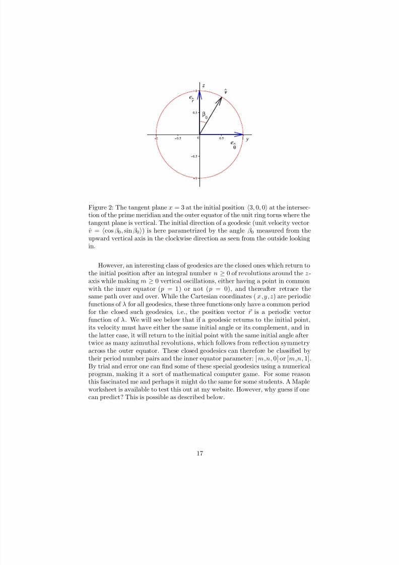
Figure 2: The tangent plane x = 3 at the initial position 3, 0, 0 at the intersec-tion of the prime meridian and the outer equator of the unit ring torus where thetangent plane is vertical. The initial direction of a geodesic (unit velocity vectorv = cos β 0, sin β 0) is here parametrized by the angle β 0 measured from theupward vertical axis in the clockwise direction as seen from the outside lookingin.

However, an interesting class of geodesics are the closed ones which return tothe initial position after an integral number n ≥ 0 of revolutions around the z-axis while making m ≥ 0 vertical oscillations, either having a point in commonwith the inner equator ( p = 1) or not ( p = 0), and thereafter retrace the

same path over and over. While the Cartesian coordinates (x,y,z) are periodicfunctions of λ for all geodesics, these three functions only have a common periodfor the closed such geodesics, i.e., the position vector r is a periodic vectorfunction of λ. We will see below that if a geodesic returns to the initial point,its velocity must have either the same initial angle or its complement, and inthe latter case, it will return to the initial point with the same initial angle aftertwice as many azimuthal revolutions, which follows from reflection symmetryacross the outer equator. These closed geodesics can therefore be classified bytheir period number pairs and the inner equator parameter: [m,n, 0] or [m,n, 1].By trial and error one can find some of these special geodesics using a numericalprogram, making it a sort of mathematical computer game. For some reasonthis fascinated me and perhaps it might do the same for some students. A Mapleworksheet is available to test this out at my website. However, why guess if one

can predict? This is possible as described below.

17

7/27/2019 torus geo


5 Energy and angular momentum: the key to

unlocking the mysteryTo understand the system of two second order geodesic equations, one canuse a standard physics technique of partially integrating them and so reducethem to two first order equations by using two constants of the motion whicharise from the two independent symmetries of the “equations of motion”: timetranslation, which results in a constant energy, and rotational symmetry, whichresults in a constant angular momentum. There is no need to understand howthis happens—it is a topic which belongs in an advanced mechanics course. Herewe will just manipulate our specific equations to accomplish our goals.

Since the mass m of the point particle whose motion traces out a geodesicpath is irrelevant in this problem, those physical quantities like energy andmomentum which involve the mass as a proportionality factor will instead by

replaced by the “‘specific” quantities obtained by dividing out the mass. Thusthe specific kinetic energy (kinetic energy 12mv2 divided by the mass m) is just

E =1

2v2 =

1

2gij

dxi

dλ

dxj

dλ(56)

=1

2

dr

dλ

2

+1

2R(r)2

dθ

dλ

2

(57)

=1

2v2 cos2 β +

1

2v2 sin2 β , (58)

and vice versav = (2E )1/2 . (59)

Both the specific energy and speed are constant for an affine parametrization of the geodesic.

In the physics approach the specific energy of the particle is constant becausefrom the point of view of its motion in space, it is only accelerated perpendicularto the surface (since the component of the second derivative along the surfacehas been designed to be zero). If a force were responsible for this acceleration,namely the normal force which keeps the particle on the surface, since it isperpendicular to the velocity of the particle it would not do any work on theparticle (recall that work done is the integral of the dot product of the forceand velocity vectors). Thus its energy and hence specific energy E must remainconstant (said to be “conserved” along the geodesic). Similarly the speed v =(2E )1/2 must therefore be constant along a geodesic according to this reasoning.

In this same physics language, the second geodesic equation tells us that the

specific angular momentum about the axis of symmetry (defined exactly as inthe case of circular motion around an axis with radius R(r), namely the velocity

vθ = R(r) dθ/dλ in the angular direction multiplied by the radius R(r) of thecircle)

= R(r) vθ = R(r)2dθ

dλ= R(r) v sin β (60)

18

7/27/2019 torus geo


7/27/2019 torus geo


Figure 3: Instead of fixing the speed/energy (circles) in the initial velocity planeat the outer equator, fixing the angular momentum leads to a vertical line corre-sponding to all geodesics in either counterclockwise ( > 0) or clockwise ( < 0)azimuthal motion or in purely radial motion ( = 0). Here the counterclockwisecase is illustrated.

This combination of the constants of the motion is of course also constant alonga geodesic, so that for initial data at (r, θ) = (0, 0) one has

R(r)sin β = R(0)sin β 0 . (66)

The obvious interpretation of this constant length is its value at a radial “turningpoint” r = r(ext) where sin β = ±1 (see below), if it exists, where the unitvelocity is aligned with the azimuthal angular direction and this reduces to±R(r(ext)). The existence of this constant is a consequence of the 1-parameterrotational group of symmetries of the torus (or indeed any surface of revolution)about its axis of symmetry, and indeed such a constant of the motion ariseswhen the surface is invariant under any 1-parameter group of symmetries, afact easily seen in the variational approach to the geodesic equations. In themathematical language, this quantity is a constant discovered by Clairaut forgeodesic motion in a surface described in a coordinate system adapted to this1-parameter group of symmetries [6, 7]. However, it appears that none of the

textbooks on differential geometry develop the tools of transformation groups orsymmetry groups (associated with the names of Lie and Killing), and so cannotremark on the interpretation available in most elementary textbooks on generalrelativity. These surfaces of revolution are invariant under the the 1-parametergroup of rotations about the symmetry axis, and as such are “isometries” of the intrinsic metric. The circular orbits of this symmetry group are the integral

20

7/27/2019 torus geo


curves of a Killing vector field generator, which in this case is ∂/∂θ. Translationsin this coordinate θ correspond to these rotations. The Clairaut conditions on

Clairaut coordinates just state that the coordinates are orthogonal and one isa Killing coordinate, i.e., such that the metric is invariant under translationin that coordinate, and hence the components of the metric in the coordinatesystem adapted to that single independent Killing vector field are independentof that coordinate. The constant of the motion is just the inner product of theunit tangent vector (unit velocity) along a geodesic with that Killing vector field

(v)θ = v · ∂

∂θ= R(r)sin(β ) . (67)

We can use this constant of the motion to answer some interesting questionsabout the crossing angle of a geodesic with the parallels it encounters. Forexample, if a geodesic starting at the outer equator crosses the inner equator,

it must do so at an angle which satisfies

sin β (λ) =R(0)

R(bπ)sin β 0 =

a + b

a − bsin β 0 =

2 + c

csin β 0 . (68)

This crossing angle β (λ) is a bigger angle than β 0 for a ring torus for which c > 0.If a geodesic starts out at the outer equator and returns to the outer equatorR(r(λ)) = R(0), then sin(β (λ)) = sin(β 0), so its crossing angle with respect tothe outer equator is either a) the same β 0 or b) its supplement π−β 0. This cross-ing angle cannot equal one of the two sign-reversed angles −β 0, −(π − β 0) sincethe azimuthal angle θ is a monotonically increasing or decreasing function alonga geodesic for nonzero angular momentum (the sign of dθ/dλ does not change),always revolving either clockwise or counterclockwise around its symmetry axis

as seen from above. If the geodesic returns to the initial starting point at theorigin of coordinates, the first case a) means the initial data at the final point isthe same as at the starting point and so it must retrace its path and the geodesicis closed, while in the second case b) by symmetry with respect to reflectionsacross the equatorial plane, the curve must be a geodesic which will return tothe starting point with the original initial velocity after another time intervalof equal length λ, and is therefore also closed. However, for geodesics whichpass through the inner equator, the radial coordinate is either monotonicallyincreasing or decreasing (dr/dλ always has the same sign, never vanishing), andso cannot cross itself at the starting point with the supplementary angle andhence must begin retracing its path as a closed geodesic. In fact since for suchgeodesics both r and θ are monotonic functions of λ, the velocity must alwaysremain within one of the four quadrants of the tangent space for which the sign

combinations of (dr/dλ, dθ/dλ) are fixed. Thus the unbound geodesics eithernever intersect themselves or they are closed and retrace their own path. Thebound geodesics may intersect themselves, but only at supplementary angleswith respect to the meridians.

The so called “turning points” of the radial motion occur at extreme radialvalues r = r(ext), where the radial velocity vr = v cos β is zero and the velocity

21

7/27/2019 torus geo


purely azimuthal. These points correspond to cos β = 0 and so sin β = ±1 andare therefore determined as the roots of the equation

R(r(ext)) = R(0)| sin β 0| , (69)

or explicitly for the torus, r(ext) = ±r(max) where

r(max)

b= χ(max) = arccos

(a + b)| sin β 0| − a

b

= arccos((2 + c)| sin β 0| − (1 + c)) . (70)

This can only hold for the so called bound geodesics (see below) for which aturning point radius R(r(ext)) exists and hence must be larger than or equal tothe inner equatorial radius

R(0)

|sin β 0

|= R(r(ext))

≥R(bπ)

↔ −πb

≤r(ext)

≤πb , (71)

so that sin β 0 is larger in absolute value than the ratio of the inner and outerequatorial radii

| sin β 0| ≥ R(bπ)

R(0)=

a − b

a + b=

c

2 + c. (72)

The formula for r(ext) can be used to aim geodesics starting at the outerequator to hit a certain extremal radius. For example, to asymptotically ap-proach the inner equator one needs the initial angle to satisfy

| sin β 0| =a − b

a + b=

c

2 + c→ β 0 = ±β (crit), π ± β (crit) (73)

where

β (crit) = arcsin c

2 + c

(74)

(19.5◦ for the unit ring torus) defines a critical angle, or to reach the Northernor Southern Polar Circles the angle must be larger and satisfy

| sin β 0| =a

a + b=

1 + c

2 + c(75)

defining another special angle

β (polar) = arcsin

1 + c

2 + c

(76)

(41.8◦ for the unit ring torus). All initial angles smaller than this correspond togeodesics which cross the polar circles, while all initial angles smaller than theformer critical angle result in unbound geodesics which cross the inner equator.

Note that one can simply solve the energy equation describing the radialmotion for the radial velocity and integrate

λ − λ0 =

rr0

1

(2E − 2/R(r)2)1/2dr . (77)

22

7/27/2019 torus geo


Figure 4: The unit angular momentum potential (i.e., for 2 = 1) for “non-radial” torus geodesics starting on the outer equator on the unit ring torus(a, b) = (2, 1), where r = χ. If the energy is less than 1/2, the geodesics donot make it through the hole: |rmax| < π. Of course the potential is periodicas well, and we have only shown one period here: −π ≤ r ≤ π. For energylarger than 1/2, the variable r is unbounded. Five energy levels are shown: 2typical bound geodesics (E < 1/2), 1 unique bound geodesic asymptotically

approaching the inner equator (E = 1/2), and 2 typical unbound geodesics(E > 1/2). The bound geodesics have symmetric extremal radii. The potentialminimum corresponds to the outer equator, and the potential maximum to theinner equator.

For the torus this integral can be done exactly in terms of elliptic functions, butthe result cannot be inverted to express r as a function of λ. However, it canalso just be integrated numerically to provide λ(r), which becomes arc lengthonce multiplied by the speed. Note also that at turning points of the radialmotion dr/dλ = 0, so that the denominator of this integral vanishes. Thusan integral for which the turning point r is an upper limit of integration is animproper integral, which even if it converges can still lead to some complications

for numerical evaluation.

23

7/27/2019 torus geo


6 The reduced problem of the radial motion

The real advantage of our physics approach is in the diagram we can createto describe the radial motion. The second term in the energy is the “effectivepotential energy” due to the angular motion, called the centrifugal potential. If we only consider nonradial motion, we can fix a convenient value of the angularmomentum while allowing the energy to be determined by the initial angle andtherefore have a single potential energy function U describe the radial motion

1

2

dr

dλ

2

+ U = E , U =1

2

2

R(r)2=

1

2

2

(a + b cos(r/b))2. (78)

Since the sum of the radial kinetic energy and this potential energy functionis the constant energy for a given geodesic, once one sets an energy level, themotion must be restricted to the region where the difference E − U is nonneg-

ative, with the radial velocity dr/dλ necessarily zero at points where E = U ,which determine the extreme values r(ext) of the radial variable within whichthe geodesic is confined. Fig. 4 illustrates one period of the periodic potentialfor the unit ring torus (a, b) = (2, 1) with the choice = 1, where the innerequator has energy 1/2 and is the unstable equilibrium solution sitting at thepeak of the potential energy graph. Geodesics with energy less than 1/2 arebound with radial motion confined between the symmetric extreme values of the radial coordinate, analogous to the negative energy elliptic orbits of theKepler problem. The geodesics with energy E > 1/2 are unbound, requiring aninfinite interval −∞ < r < ∞ of radial coordinate values to describe continu-ously, and therefore the periodic potential shown in Fig. 5. For example, theenergy E = 3.942 corresponds to the 7 loop unbound geodesic shown in Fig. 6for the initial angle β 0 = 0.119 radians (6.8◦).

If we return to the original second order equation for the radial variable andreplace the angular velocity using conservation of angular momentum we get

d2r

dλ2= R(r)R(r)

dθ

dλ

2

= R(r)R(r)

R(r)2

2

=2R(r)

R(r)3= −dU

dr. (79)

This shows that the effective potential really does generate the radial componentof the effective (specific) force through its derivative. However, we are sparedhaving to deal with this second order equation since we have its first integralalready, namely the energy relation. Note that this effective force is really

just the radial coordinate acceleration required to keep the geodesic directionunchanged and is not a true force. The only real force on the motion (if this werea real point particle in motion) is the force normal to the surface required tokeep the curve from leaving the surface, a force which arises from the constraint

that the motion remain within the surface. For completeness we show thatthe constancy of energy implies the second order radial equation by a simplederivative calculation. If the energy is constant but r is not constant, then

E =1

2

dr

dλ

2

+1

2

2

R(r)2,

dE

dt=

dr

dλ

d2r

dλ2− 2R(r)

R(r)3

. (80)

24

7/27/2019 torus geo


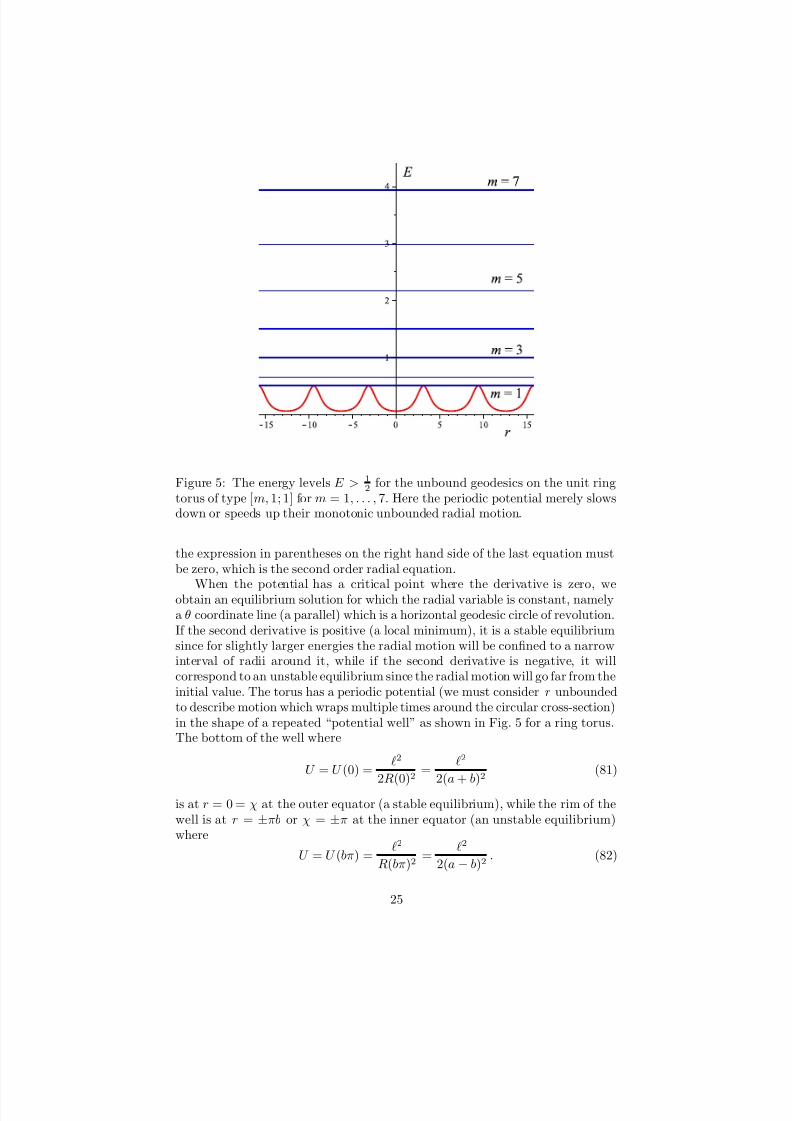
Figure 5: The energy levels E > 12 for the unbound geodesics on the unit ring

torus of type [m, 1; 1] for m = 1, . . . , 7. Here the periodic potential merely slowsdown or speeds up their monotonic unbounded radial motion.

the expression in parentheses on the right hand side of the last equation mustbe zero, which is the second order radial equation.

When the potential has a critical point where the derivative is zero, weobtain an equilibrium solution for which the radial variable is constant, namelya θ coordinate line (a parallel) which is a horizontal geodesic circle of revolution.If the second derivative is positive (a local minimum), it is a stable equilibriumsince for slightly larger energies the radial motion will be confined to a narrowinterval of radii around it, while if the second derivative is negative, it willcorrespond to an unstable equilibrium since the radial motion will go far from theinitial value. The torus has a periodic potential (we must consider r unboundedto describe motion which wraps multiple times around the circular cross-section)in the shape of a repeated “potential well” as shown in Fig. 5 for a ring torus.The bottom of the well where

U = U (0) =2

2R(0)2=

2

2(a + b)2(81)

is at r = 0 = χ at the outer equator (a stable equilibrium), while the rim of thewell is at r = ±πb or χ = ±π at the inner equator (an unstable equilibrium)where

U = U (bπ) =2

R(bπ)2=

2

2(a − b)2. (82)

25

7/27/2019 torus geo


Figure 6: An closed geodesic [7, 1; 1] for the unit ring torus with 7 loops crossingthe inner equator, corresponding to an initial angle of β ≈ 0.119 (≈ 6.81◦) andrelatively high energy E = 3.942 on the unit ring torus.

The “walls” of the potential act as a barrier to reaching the inner equator unlessthe energy is sufficiently high to overcome this barrier. The turning pointsr = r(max), r(min) of the radial motion for this case occur at the minimum radiusR(r) allowed by conservation of angular momentum: where the energy levelintersects the potential graph. The maximum angular velocity dθ/dλ occurs atthese turning points where the radial velocity is momentarily zero, simply by

conservation of angular momentum since these points turning are closest to thesymmetry axis about which the geodesic is revolving. For the horn torus, therim of the potential well moves up to positive infinity, so that the nonradialunbound geodesics disappear.

By fixing the angular momentum, one can consider a single potential functioninstead of a family at the cost of allowing the variable energy to describe differentgeodesics. For example, if we consider an initial point at the origin of coordinateson the outer equator (see Fig. 3), we only have to vary the angle of the directionof the velocity to describe the 1-parameter family of distinct geodesic pathswhich emanate from the initial position, and the different inclination anglescorrespond to the different values of the energy (equivalently of the speed).There are a number of obvious choices to fix = 0 in the potential functionwhich only depend on the shape parameter

U =2

2R(r)2=

2

2(a + b cos(r/b))2=

2/b2

2(c + 1 + cos(r/b))2. (83)

For example, setting || = R(0), R(bπ), b or equivalently ||/b = (a + b)/b, (a −b)/b, 1 = c + 1, c, 1 leads to values at the outer and inner equators respectively

26

7/27/2019 torus geo


of

U (0) = 12

, 12

c

c + 2

2

, 12(c + 2)2

, U (bπ) = 12

c + 2

c

2

, 12

, 12c2

. (84)

The middle choice won’t work for horn tori where c = 0. For the unit ring torus(c = 1) either of the last two choices are the same as simply setting || = 1,which will be assumed below in the unit ring torus examples.

This latter potential is illustrated in Figs. 4 and 5 for the unit ring torus.Those orbits for which |χ(max)| ≤ π are referred to as the bound orbits sincethe range of the radial variable is confined to a finite interval of values whichis symmetric about the center r = 0 because of the reflection symmetry of the potential about its center. In the physics language, the bound geodesicsare “trapped” in the potential “well,” while the unbound geodesics are freeto pass from one well to the next as they continue to loop around the torus

forever. For the energy level 12 , there are two geodesics. One is the innerequator which is an unstable equilibrium, and the other is a geodesic whichasymptotically approaches the inner equator both from above and from belowat the two limiting turning points of the radial motion, revolving an infinitenumber of times around the symmetry axis in each direction. If the energyis larger than 1

2 , the orbits are referred to as unbound since one requires anunbounded range of the radial variable to describe them continuously. Notethat only the inner equator geodesic does not pass through the outer equator(obviously!), so initial data at a point on the outer equator is enough to describeall other geodesics.

Thus from the potential diagram typical of all ring tori, one sees five classesof geodesics: the inner and outer equators, the geodesic asymptotic to the innerequator, the remaining bound geodesics, and the unbound geodesics, to which

we must add the sixth type, namely the radial geodesics since the radial coor-dinate lines are geodesics for any surface of revolution, as they must be becauseof the reflection symmetry about the plane cross-section of the surface whoseintersection is the given radial coordinate line.

On the other hand when one passes from ring tori to the horn torus bydecreasing the shape parameter c to zero, the energy level for the inner equatorgrows to positive infinity and the nonradial unbound geodesics disappear. Allgeodesics are trapped in the infinite potential well whose walls go to infinityat the inner equator where R(r) = 0. Continuing into the spindle tori, onehas two separate sets of nonradial bound geodesics confined either to the appleor the lemon component of the torus, and the two points of self-intersectionare protected by the infinite potential walls surrounding the axis of symmetry.The infinite values of the potential occur at

±r∞/b =

±χ∞ where R(r∞) = 0,

namelyχ∞ = arccos (−a/b) = arccos(−(c + 1)) . (85)

There are two stable equilibrium solutions, one at the inner equator on the lemonand one at the outer equator on the apple. These potentials are illustrated inFig. 7, where the condition ||/b = 1 is assumed so that U (0) = 1/2(c + 2)−2 <

27

7/27/2019 torus geo


Figure 7: The potential for the (a,b,c) = (1, 1, 0) unit horn torus (left) on theinterval −π ≤ r ≤ π and for the (a,b,c) = (1/2, 1, −1/2) spindle torus (right)on the interval −2π ≤ r ≤ 2π. The horn torus has a single equilibrium solutionat the outer equator at the origin, with infinite potential walls surrounding theinner equator. The spindle torus has equilibrium solutions at both the outer(apple) equator (center well) and the inner (lemon) equator (outer wells), andnonradial geodesics are confined to either the lemon or spindle. Turning pointsfor one energy level are shown for both cases.

1/2 and U (bπ) = 1/2c−2 > 1/2. As one decreases c from 0 towards −1 the innerwell narrows and rises as χ∞

→π/2 and the outer well widens and deepens,

until at the limiting case c = −1 of the sphere, the inner and outer wells arethe same shape, and only the inner well is needed to describe the nonradialgeodesics, all of which are bound and closed with −π/2 < r < π/2. Note thatif we allow −b < a < 0 or −2 < c < −1, then we again get the spindle toribut with r = 0 now describing the inner equator on the lemon surface. Thisallows one to describe the lemon geodesics using initial data at the origin of coordinates (r, θ) = (0, 0) as in the remaining cases.

Since the outer equator is a stable equilibrium, nearby geodesics will oscillateabout it with a frequency that is easily calculated by approximating the bottomof the potential well by its quadratic Taylor polynomial. The equations of motion for these limiting solutions are then

r = 0 :

dθ

dλr=0 =

(a + b)2 → θ =

(a + b)2 λ ,

r 1 : E =1

2

dr

dλ

2

+2

(a + b)2+

2r2

2b(a + b)3,

having imposed the initial condition θ = 0 at λ = 0 on the angular solution.

28

7/27/2019 torus geo


Figure 8: Periodic orbits [3, 2; 1] (left, unbound) and [3, 2; 0] (right, bound) forthe unit ring torus corresponding to an initial angles of β 0 = 0.0.3226 (18.5◦)and β 0 = 0.7167 (41.1◦).

Defining

ω =||

[b(a + b)3]1/2,

1

2R2 = E − 2

(a + b)2(86)

the energy equation describes a simple harmonic oscillator

R2 =

dr

dλ

2

+ ω2r2 . (87)

Integrating this for λ as a function of r (solve for dλ and integrate), imposingthe initial condition λ = 0 at r = 0 yields the result

r =±R

sin(ωλ) =±R

sin((c + 2)1/2θ) . (88)

Thus there are (c + 2)1/2 radial oscillations during one revolution about thesymmetry axis, or

√ 3 ≈ 1.73 for the unit ring torus. The final equation here,

having eliminated the parameter λ, directly gives the orbit equation for this case,namely the path traced out by these limiting geodesics near the outer equator.Note that the smallest positive integer value of the positive shape parameterthat leads to an asymptotically closed orbit for the small oscillations at the outerequator is c = 2 (i.e., a/b = 3), with 2 oscillations per revolution. For a sphere(limiting value c = −1) this leads to one oscillation per revolution, correspondingto a great circle, which also characterizes the exact oscillations about the equatorof any amplitude. For the redundant parameter range −2 < c < −1 for spindletori (duplicating the range −1 < c < 0) where r = 0 instead corresponds to theinner equator (on the lemon) of the self-intersecting torus, one finds an infinitenumber of values of c for which the periodic limiting small amplitude oscillationshave a period which is an integer multiple of the length of the inner equator.

29

7/27/2019 torus geo


7 The orbits

If we are only interested in the paths traced out by the geodesics (the orbits), wecan easily eliminate the affine parameter λ and get a direct integral relationshipbetween θ and r in general, first solving the energy equation for the radialvelocity and then using the chain rule

dθ

dr=

dθ

dλ/

dr

dλ=

R(r)21

(2E − 2/R(r)2)1/2=

R(r)

1

(2ER(r)2 − 2)1/2. (89)

Note that this goes infinite at a turning point of the radial motion where dr/dλ =0. This expression can be integrated and expressed in terms of the initial dataat (r, θ) = (0, 0) parametrized by the initial polar angle β 0 by using the relation

E =2

2R(0)2

sin2

β 0, (90)

which leads to

θ =

r0

R(0)sin β 0

R(r)(R(r)2 − R(0)2 sin2 β 0)1/2dr ≡ F (r, β 0)

=

χ0

(c + 1) sin β 0

(c + 1 + cos χ)[(c + 1 + cos χ)2 − (c + 1)2 sin2 β 0]1/2dχ

≡ G(χ, β 0) . (91)

Since this integral cannot be done in closed form unless c = −1 (the limitingcase of a sphere), one must numerically integrate this. Introduce the reciprocalof the angle θ measured in cycles (i.e., the reciprocal of θ/(2π))

N (χ, β 0) =2π

G(χ, β 0), β 0 < β (crit) . (92)

This can be used to numerically determine the values of the initial angle β 0which correspond to closed orbits.

For an unbound geodesic the value of this quantity after one radial oscillationis the theta frequency function N (2π, β 0) = 2π/G(2π, β 0) associated with thetheta period G(2π, β 0). This quantity is the number of times the azimuthalincrement occurring during that complete oscillation fits into a full azimuthalrevolution, i.e, the number of radial oscillations per azimuthal revolution. If this is a rational number m/n

N (2π, β 0) =

m

n , (93)

then after m radial oscillations, n azimuthal revolutions will take place, cor-responding to an unbound geodesic of type [m, n; 1]. Fig. 9 shows a plot of N (2π, β 0) over the entire interval β ∈ [0, β (crit)) of values corresponding to theunbounded geodesics moving up initially in the positive θ direction. The graph

30

7/27/2019 torus geo


Figure 9: The number N (2π, β 0) of radial oscillations per azimuthal revolutionfor the unbound geodesics on the unit ring torus plotted versus the initial an-gle β 0 first over the interval [0, β (crit)] and then for [0.9999β (crit), β (crit)], whereβ (crit) ≈ 0.3398. The dashed line shows the asymptotic k/β 0 approximation forsmall angles. The rational values N (2π, β 0) = m/n correspond to the unboundclosed geodesics of type [m, n;1].

rises very quickly due to a vertical asymptote at β 0 = 0, while it decreasesextremely slowly to its limiting value limβ0→β(crit) N (2π, β 0) = 0 where it ap-proaches a vertical tangent, as shown in a closeup of the endpoint behavior.

The integral F (π, β (crit)) is an improper integral whose integrand denomina-

tor goes to zero at the right endpoint, and it has an infinite value correspond-ing to the infinite number of azimuthal revolutions which occur as the criticalgeodesic asymptotically approaches the inner equator. The reciprocal N (π, β 0)therefore goes to zero as β 0 → β (crit) from the left, but very slowly. To get anidea of how slowly, set β 0 = β (crit) (which satisfies (c + 1) sin β (crit) = c), andevaluate the Taylor expansion about χ = π of the reciprocal of the integrandof F (π, β (crit))/(2π) to find that the leading behavior of the integrand at itsendpoint χ = π is

1

2πc1/2(π − χ)(94)

so its antiderivative behaves like

1

2πc1/2

ln[(π

−χ)−1] . (95)

Thus if in the discrete numerical plotting of this function at the endpoint, if thelast sampled point is π − χ = 10−10, say, then the value of the antiderivativethere for the unit ring torus (c = 1) is only about

1

2πln[(π − χ)−1] ≈ 3.3 . (96)

31

7/27/2019 torus geo


Figure 10: The number N (2π, β 0) of radial oscillations in one azimuthal revo-lution versus the initial angle β 0 ∈ (β (crit), π/2], here shown for the unit ring

torus with the upper bound N (2π,π/2) = (c + 2)1/2

= √ 3 ≈ 1.73. The ratio-nal values N (2π, β 0) = m/n correspond to the bound closed geodesics of type[m, n; 0] with m radial oscillations during n azimuthal revolutions.

The reciprocal of this gives a rough idea of the value of N reached by this lastsampled point. This means numerically finding rational values of N for evenrelatively large proper fractions where β 0 is close to the critical value will bedifficult. For example, for the unit ring torus where β (crit) ≈ 0.3398369094(19.471◦), one easily finds β 0 = 0.2382795502 (13.7◦) for the [3, 1; 1] geodesicsand β 0 = 0.0.3226432999 (18.5◦) for the [3, 2; 1] geodesics, but the result β 0 =0.0.3226432999 (19.454◦) for the [3, 4; 1] geodesic takes a considerable time,while the value β 0 = 0.3395532232 (19.469◦ for the [3, 5; 1] geodesic takes too

long for a simple root finder to obtain and one must resort to trial and error.The azimuthal integral θ = G(χ, β 0) for the orbits of the unbound geodesicscan be easily approximated in the limit of very small initial angles where a smallincrement of the azimuthal angle occurs during one radial oscillation. Under

32

7/27/2019 torus geo


the condition /√

2E = (a + b)sin β 0 1, the integral approaches

θ = χ0

√ 2E

b dχR(bχ)2

, (97)

which has a complicated exact value but the increment over one revolution−π ≤ χ ≤ π is relatively simple (computer algebra system exercise)

∆θ =2πab(a + b)

(a2 − b2)3/2β 0 . (98)

This leads to

β 0 → 0 : N (2π, β 0) → (a2 − b2)3/2

ab(a + b)

1

β 0=

c3/2(c + 2)1/2

(c + 1)

1

β 0, (99)

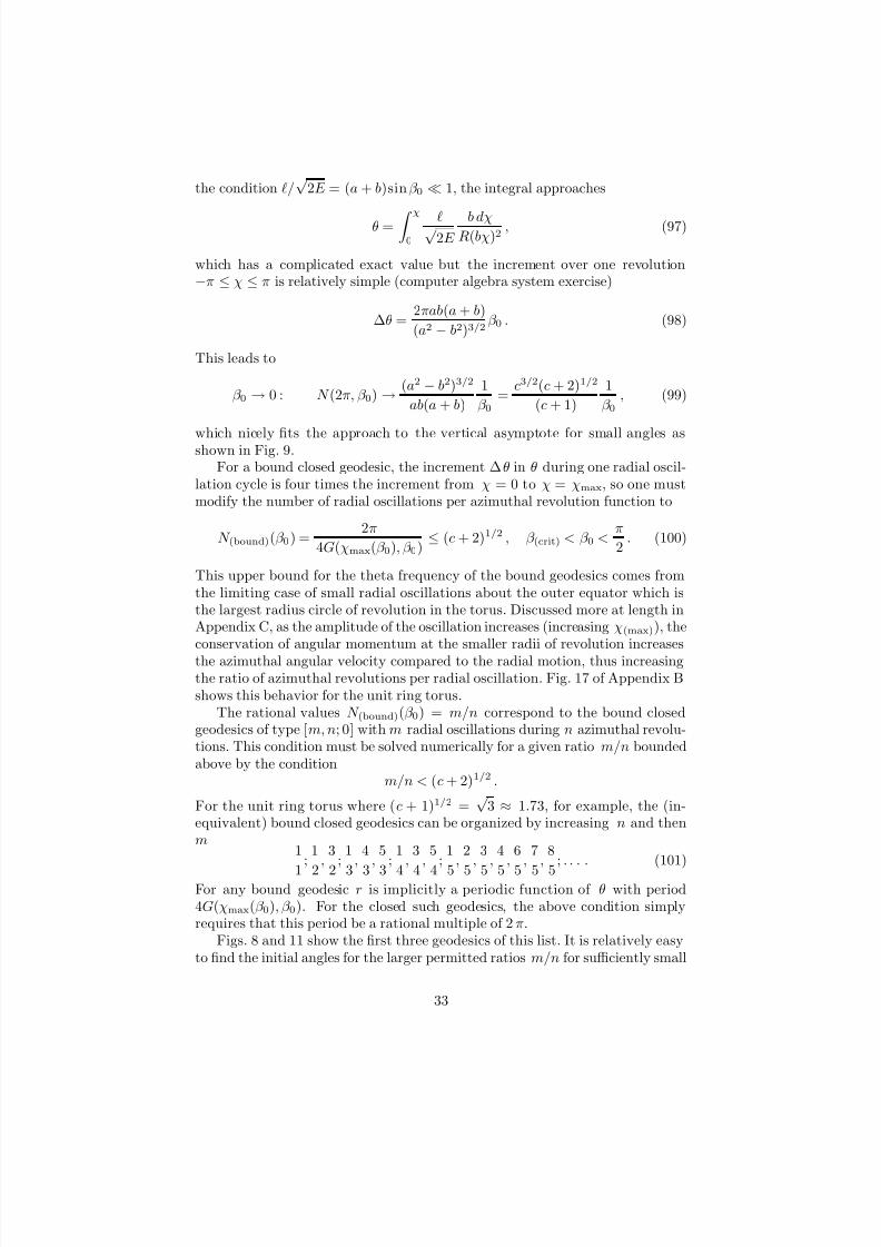
which nicely fits the approach to the vertical asymptote for small angles asshown in Fig. 9.For a bound closed geodesic, the increment ∆θ in θ during one radial oscil-

lation cycle is four times the increment from χ = 0 to χ = χmax, so one mustmodify the number of radial oscillations per azimuthal revolution function to

N (bound)(β 0) =2π

4G(χmax(β 0), β 0)≤ (c + 2)1/2 , β (crit) < β 0 <

π

2. (100)

This upper bound for the theta frequency of the bound geodesics comes fromthe limiting case of small radial oscillations about the outer equator which isthe largest radius circle of revolution in the torus. Discussed more at length inAppendix C, as the amplitude of the oscillation increases (increasing χ(max)), theconservation of angular momentum at the smaller radii of revolution increases

the azimuthal angular velocity compared to the radial motion, thus increasingthe ratio of azimuthal revolutions per radial oscillation. Fig. 17 of Appendix Bshows this behavior for the unit ring torus.

The rational values N (bound)(β 0) = m/n correspond to the bound closedgeodesics of type [m, n; 0] with m radial oscillations during n azimuthal revolu-tions. This condition must be solved numerically for a given ratio m/n boundedabove by the condition

m/n < (c + 2)1/2 .

For the unit ring torus where (c + 1)1/2 =√

3 ≈ 1.73, for example, the (in-equivalent) bound closed geodesics can be organized by increasing n and thenm

1

1

;1

2

,3

2

;1

3

,4

3

,5

3

;1

4

,3

4

,5

4

;1

5

,2

5

,3

5

,4

5

,6

5

,7

5

,8

5

; . . . . (101)

For any bound geodesic r is implicitly a periodic function of θ with period4G(χmax(β 0), β 0). For the closed such geodesics, the above condition simplyrequires that this period be a rational multiple of 2π.

Figs. 8 and 11 show the first three geodesics of this list. It is relatively easyto find the initial angles for the larger permitted ratios m/n for sufficiently small

33

7/27/2019 torus geo


Figure 11: Bound periodic orbits [1, 1; 0], [1, 2; 0] for the unit ring torus corre-sponding to initial angles of β 0 ≈ 0.4097, 0.3422(≈ 23.5◦, 19.6◦) and maximumradius χmax ≈ 143.6◦, 173.4◦ and lengths 15.3, 21.9. Orbits with initial an-gle β 0 ≤ 41.8◦ reach the North Polar Circle, while orbits with initial angleβ 0 ≤ 19.47◦ are unbound, passing the inner equator if the inequality is satisfied.

integers, but as the ratio m/n gets smaller, the limiting vertical tangent in thegraph of N (bound)(β 0) as β 0 → β (crit) from the right creates problems for accuratedetermination of the roots where N (bound) is a small rational number. Becauseits reciprocal is an improper integral with a positive integrand that goes toinfinity at the critical angle, numerical evaluation will underestimate the resultof the integral (because numerically it will only sense some highest value of the integrand in the discrete approximation and miss the infinite contribution).Thus the true angle which gives a particular rational value to N (bound)(β 0) willhave to be a bit bigger to compensate for the lower value of the approximateintegral. Thus one can take this underestimate as a starting angle in the fullnumerical geodesic solver and increase it slightly by trial and error until onecloses the orbit. Even for larger values of the ratio m/n where one can accurately

determine the corresponding initial angle, if m or n gets too large, one is of course limited again by numerical error in the full geodesic solver since toomany radial oscillations or azimuthal revolutions translates into accumulatednumerical error, so the orbit may not appear to close. When it fails to close by

just a little, one sees a constant rate of “precession” of the node (where the orbitcrosses the outer equator r = 0) since the crossing angle at the outer equator isthe same each time it crosses nearby and hence it repeats the original trajectorybut translated around the torus slightly by the amount by which the returnposition to the outer equator misses the original meridian of its departure. Thisis illustrated in Fig. 12.

8 Lengths of geodesics

Since increments of the affine parameter are only proportional to the arc lengthof a geodesic segment, one must evaluate the arc length from the affine parameterincrement using the constant of proportionality (2E )1/2, which is a functionof the energy or equivalently of the initial angle. If one has only incompleteinformation not including the affine parameter increment, like the initial angle

34

7/27/2019 torus geo


Figure 12: An almost closed bound geodesic close to the [7, 5; 0] closed geodesic(β 0 = 0.6124, 35.08 degrees) with a slightly higher initial angle (β 0 = 0.614,35.18 degrees) that causes the geodesic to return to the outer equator nearthe initial meridian a bit too soon, and therefore causing the nodal point of return near the initial meridian to precess in the opposite direction of the orbit(the orbit increases the azimuthal angle, the precession decreases the azimuthalangle of the node). A slightly smaller initial angle would lead to precessionin the same direction as the orbit. Trial and error adjustment of the (slightlysmaller) approximate initial angle from the integral condition enables one to

narrow in on the correct value to as many digits as one has patience for, subjectto the unknown accuracy of the numerical integration scheme of course.

for a closed geodesic, the arc length integral remains to be evaluated, say asa function of the interval of radial coordinate values describing the geodesicsegment. The corresponding affine parameter integral given in Eq. (77) can beevaluated exactly in term of elliptic functions, but the resulting complicatedformula is not very enlightening. With a slight modification, this formula maybe used to evaluate the arc length of one complete period of the motion for aclosed geodesic.

To evaluate the arc length of one period of one of the unbound closedgeodesics of the class [m, n; 1], one can first evaluate the arc length of one radialloop (0

≤r

≤2πb or 0

≤χ

≤2π) and then multiply by the number m of radial

loops. The arc length of one radial loop follows from integrating

ds

dr=

ds/dλ

dr/dλ=

(2E )1/2

dr/dλ, (102)

35

7/27/2019 torus geo


namely

L =

2πb

0

(2E )1/2 dr(2E − 2/R2)1/2

= b

2π

0

R dχ(R2 − 2/(2E ))1/2

= b

2π0

R dχ

(R2 − R(0)2 sin2 β 0)1/2. (103)

For example for the 7 loop geodesic with energy E = 3.942 on the unit ringtorus, the length of one loop is 6.45 and of the entire 7 loops: 45.12. Thiscompares to the circumferences of the inner equator, the Polar Circles andthe outer equator: [2π(1), 2π(2), 2π(3)] ≈ [6.28, 12.57, 18.85]. These integralsare easily done numerically with a computer algebra system. Notice that forvery high energy (very small initial angle β 0 → 0), this reduces to the radialcircumference of the torus.

For any bound geodesic, one can easily evaluate the length of one transitdeparting from the initial point on the outer equator, traveling to a given turningpoint, returning to cross the outer equator and going to the other turning pointand back again by taking 4 times the length from the outer equator to oneturning point

L = 4 b

χ(max)

0

R dχ

(R2 − R(0)2 sin2 β 0)1/2, (104)

whereχ(max) = arccos ((2 + c)| sin β 0| − (1 + c)) . (105)

For example the [1,1;0] closed geodesic shown in Fig. 11 on the unit ring torushas length 15.26.

One can also categorize the closed geodesics by the number of self-intersec-

tions they exhibit, as initiated by Irons [3]. To examine geodesic crossingswithout trying to follow a geodesic around the 3-d torus in rotatable computergraphics images, it is useful to map the torus onto the unit square by introducingtwo angles measured in cycles rather than radians

(Ξ, Θ) =

χ

2π,

θ

2π

, with 0 ≤ χ, θ ≤ 2π −→ 0 ≤ Ξ, Θ ≤ 1 . (106)

For comparison the grid of all positive pairs [m, n] describing the distinctclosed geodesics of the flat torus is briefly discussed in the Appendix. Like theflat torus, the [m, n; 1] closed geodesics on a ring torus exist for all positivepairs (m, n) and have no self-intersections, but the [m, n; 0] closed geodesics areconstrained by the theta frequency condition m/n < (c + 2)1/2 of the limiting

geodesics near the outer equator, which have the largest period of the boundgeodesics, and self-intersections are allowed. As one gets closer and closer tothe critical geodesic which asymptotically approaches the inner equator, thecloseness to the unstable equilibrium there allows an arbitrarily large numberof azimuthal revolutions near it before the geodesic flies off towards the outerequator again, which can be arranged to happen to hit any point on the outer

36

7/27/2019 torus geo


equator. Thus one can get all pairs (m, n) for m/n → 0. Numerically this isproblematic, however, since numerical error is hard to control near an unstable

equilibrium.Given that only the bound geodesics can have self-intersections, comparison

of the low integer geodesics of type [m, n; 0] reveals the following apparent cross-ing rules as a function of the number m of radial oscillations. For the boundgeodesics on the unit ring torus starting at the origin of coordinates with initialangle β ∈ (β (crit), π/2) orbiting in the increasing θ direction, looking down fromabove at the upper hemitorus one finds by inspection of many cases either 0, 1,or 2 equally spaced series of self-crossings at 0, 1, or 2 distinct values χ× of theradial angle χ ∈ [0, χ(crit)]. The equal spacing increment is 2π/m.

n = 1: No self-crossing point radii.n = 3: 1 self-crossing point radius: χ×. The series is shifted right from θ = 0

by (2π/m)/4.n > 3 odd: 2 self-crossing point radii: χ×1 < χ×2. The 2 series are shifted

right/left from θ = 0 by (2π/m)/4.n = 2: 1 self-crossing point radius χ× = 0.n > 2 even: 2 self-crossing point radii: first series at χ×1 = 0, second series

χ×2 shifted right from θ = 0 by (2π/m)/2.

It would be nice to understand how these rules come about, and to evaluate theangles χ× at which these crossings occur.

Finally while it is convenient to describe a geodesic as the curve betweentwo points which minimizes the distance between them on the surface, it isalso important to recognize that the converse is not true. While a geodesicconnecting two points is a critical point of the arc length function on the space of

paths between the two specified points, as follows from the variational approachto this problem, there can be many geodesics of differing lengths connecting anytwo points on a surface. In the flat plane, the geodesic is the unique straightline between two points, but on a sphere although there is a unique great circlecontaining any two non-antipodal points, there is still a choice of the longer orshorter segment of the great circle to follow from one point to the other, andfor antipodal points there are an infinite number of great circles to choose from.For the torus the situation is even more extreme: through any two points on thetorus, there are an infinite number of both bound and unbound geodesics whichconnect them. However, for most point pairs there is still a minimal lengthgeodesic connecting them. While one can try to aim a geodesic departing fromthe first point to hit the target point using trial and error, it is interesting thata completely different approach can be taken to numerically converge on this

connecting path [16].An interesting illustration of the minimal geodesic question regards the min-

imal length geodesic which connects two distinct points on the outer equa-tor. According to the approximate analysis above, geodesics departing from(r, θ) = (0, 0) with an initial angle differing very little from β = ±π/2 oscillateabout the outer equator with half period ∆θ = π/(c + 2)1/2, thus returning

37

7/27/2019 torus geo


to the outer equator first at θ = ∆θ. Examining numerical geodesics for suchinitial conditions then shows that for the actual geodesics, as the amplitude of

the radial oscillation increases, the actual half period increases slowly, so thatthe return point migrates slowly beyond θ = ∆θ, but the length of this geodesicsegment remains smaller than the length of the direct route between the end-points along the outer equator. Thus for two points on the outer equator withseparation equal to or less than the half period ∆θ, the outer equator segmentbetween them is the shortest geodesic between them, but for points with separa-tion greater than this critical length, the shortest geodesic is instead a half radialoscillation connecting the two points. Antipodal points on the outer equator arethe extreme case of this type, where the [1, 1; 0] geodesic which connects thosepoints is significantly shorter than half the circumference of the outer equator.

The horizontal “focusing” of the bound geodesics which emanate from theorigin of coordinates on the outer equator, like the crossing of great circles onthe sphere at antipodal points, is a consequence of the positive curvature of the torus on the outer ring between the Northern and Southern Polar Circles.On the inner ring between these Polar Circles, the curvature is negative andgeodesics from the outer equator which reach this region instead diverge fromone another before crossing on the inner equator due to the topology of thetorus. These geodesics begin crossing each other at the critical length Lr = πbequal to half the radial circumference of the torus, compared to the azimuthalcritical length Lθ = (a + b)∆θ = π(a + b)/(c + 2)1/2, leading to the ratioLθ/Lr = (c + 2)1/2. Irons [3] has evaluated the various curvature quantities onthe torus, but curvature is a long story that cannot be told here.

9 Kepler problem?

The beauty of mathematics is that many seemingly different problems actuallyshare the same mathematical foundation and hence can be treated with thesame methods to understand them. From geodesics on these special surfacesof revolution, by relaxing the condition grr = 1 to grr = f (r) we can easilyconsider general surfaces of revolution for which the radial coordinate does notmeasure arc length [5]. This enables us to handle the simple parabolic surface of revolution z = x2 + y2 = r2, for example, where grr = 1 + 4r2. However, we canalso handle the simplest example of a surface of revolution, the flat plane z = 0,but in the framework of polar coordinates, where resolving the geodesic equa-tions to reproduce straight lines is complicated but doable. Polar coordinatesare simply not adapted to the geodesic structure of the flat plane. The realpayoff, however, is to consider the simple addition of an external rotationallysymmetric force to these same flat plane equations, enabling us to handle thenonrelativistic Kepler problem with the same approach, and indeed the closelyrelated relativistic Kepler problem of planar motion in a spherically symmetricvacuum gravitational field arising either from a spherical body or a black hole.In both cases, the polar coordinates are essential to resolving the equations of motion.

38

7/27/2019 torus geo


¡

¢

£ ¤

¥

¦ §

¨

© §

£

©

¥

¨

¨

¥

¨

¡

Figure 13: A typical Kepler potential for the nonrelativistic (Newtonian gravity)and relativistic (general relativity) cases, showing the “centrifugal barrier” nearthe source (small r). Circular orbits occur at the extrema of the potential.Bound orbits have energy E < 0, while unbound orbits have E ≥ 0. Therelativistic potential turns over close to the source where stronger gravitationalattraction overcomes the centrifugal force. The lowest two energy levels showncorrespond to bound orbits with a minimum and maximum radius, while theupper two are unbound, but in the relativistic case, the highest energy levelorbit overcomes the centrifugal barrier and is captured by the source, while the

next lower energy orbit is reflected from the centrifugal barrier at the minimumradius in both cases (the outer portion for the relativistic case); the relativisticcase also contains “trapped” orbits inside the barrier.

For the flat plane case R(r) = r and the energy equation becomes

E =1

2

dr

dλ

2

+1

2

2

r2. (107)

To incorporate an actual rotationally symmetric radial force F r(r) = −dU r(r)/drinto the mix, we just need to add its potential U r(r) to the effective potentialterm already present

E =1

2

dr

dλ

2

+1

2

2

r2+ U r(r) . (108)

The new total potential then governs the problem in the same way that theeffective potential alone did the job in our previous discussion. With a potential

39

7/27/2019 torus geo


of the form

U r(r) =−

k1

r −k2

r3 →F r(r) =

−k1

r2 −3k2

r4, (109)

we can handle the nonrelativistic Kepler problem for motion in an inverse squareforce if k2 = 0 (attractive like gravitation if k1 > 0) or the relativistic Keplerproblem (k1 > 0, k2 > 0, see [11]), see Fig. 13. The additional inverse cubicpotential term in the latter case corresponds to an additional inverse quarticforce that is responsible for the precession of the orbits which in its absence areconic sections.

Amusingly enough, the radial oscillations about the outer equator of thetorus are directly mirrored in the Kepler problem, and the frequency one cal-culates for the oscillations about a stable circular orbit is called the epicyclicfrequency, an important astrophysical quantity. While these more general prob-lems are as easily dealt with as the torus geodesics, they are perhaps best left toa more comprehensive discussion elsewhere [13]. However, a slight adjustmentof the Maple worksheet for the torus allows experimentation with these kindsof orbits as well. With a little more work, one can include a light pressure dragforce to model the effect of stellar radiation pressure on orbiting dust particles,the so called Poynting-Robinson effect [14].

Perhaps the most important concept highlighted here that is missing in mostundergraduate mathematics programs is energy. There is usually just no time inan introductory course on differential equations to introduce it (and the standardtextbooks do not mention it), so whatever vague idea mathematics studentshave of it from high school or possibly from college freshman physics is neverconnected concretely to differential equations and the natural way it arises there.Even in the present article, we have danced around this connection withoutdirectly confronting it either, but hopefully its utility at least in this problem

is clear. The usual approach to geodesics through a variational approach isthe natural way to make this connection [15]. This is an interesting advancedtopic either for an undergraduate mathematics or physics setting. For advancedundergraduate mechanics in the physics setting, this approach to constrainedmotion (motion on a surface) is a natural gateway for understanding the toolsof general relativity, as developed by Walecka [2], for example.

10 What next?

It would be sad to shine the light on an interesting problem and completelyexhaust its potential for entertainment. There is much left to explore. On themathematical side, the spectrum of closed geodesics on the torus depends on theshape parameter. Passing to the horn torus c = 0 from the ring tori, the localmaximum in the periodic potential at the inner equator moves off to infinity,and the unbound nonradial geodesics disappear. All the nonradial geodesics arerepelled from the single point inner equator by this angular momentum barrier.For two-point self-intersecting tori −1 < c < 0, this infinite angular momentumbarrier splits into two barriers surrounding the two self-intersection points on

40

7/27/2019 torus geo


the symmetry axis, leading to two disjoint families of nonradial bound geodesics,those confined to the outer apple surface and those confined to the inner lemon

surface. For the shape parameter c = 2 (for example: (a, b) = (3, 1) so theratio of the outer equator radius to inner equator radius is 2), exactly two radialoscillations about the outer equator fit into one azimuthal revolution in the limitof zero amplitude oscillations. This means that for nonzero amplitudes wherethe exact frequency will be slightly different from 2, the nodal points where theoscillations intersect the outer equator will slowly migrate or “precess” in thephysics language. What is the precession frequency? This can be analyzed bykeeping the next term beyond the quadratic one in the Taylor expansion of thepotential about its minimum. (Similarly one can try to analyze the precessionof the node for near miss closed geodesics to calculate the incrementing angleof precession described above.) For the pinched torus, all radial geodesics passthrough the pinching point at the origin, but all of them have a vertical tangentvector, so one looses uniqueness of the initial value problem for the geodesicsthere; one can match up radial geodesics of different azimuthal angle on eitherside of the pinching point. What does this do to the torsion and differentiabilityof those curves?

On the physical side, one can easily explore motion in various classical me-chanical force potentials as hinted at for the Kepler problems. In an advancedmechanics course, where only formula manipulation was possible when I was astudent, there are exciting possibilities for student experimentation.

Finally the obvious must be pointed out. None of this would be possiblewithout the incredible tool now at the disposal of faculty and students alike:the computer algebra system on our personal computers. Both of the two leadingsuch software packages Maple and Mathematica offer to motivated students anenormous potential for exploring mathematical and physical problems, if given

a little guidance from faculty. The problem for undergraduate teaching is tofind the opportunities to engage students in picking up this tool in parallel withtheir gradual increase in theoretical sophistication in either a mathematics orphysics setting.

A The flat torus closed geodesics

For comparison it is useful to consider the spectrum of closed geodesics for thesimpler flat torus. The simplest realization of the flat torus is the plane withpoints identified if their Cartesian coordinates differ by integers, thus reducingdistinct points to the unit square in the first quadrant with opposite boundaryline segments identified. One can classify these geodesics by the pair of periods[m, n] of the number of revolutions in the horizontal and vertical directionsrespectively. Fig. 14 shows a typical geodesic of type [2, 3] through the originreturning the origin at the point (2, 3) in the plane, with length

√ 22 + 32 =

√ 13.

Fig. 15 shows in the same way a representation of the lattice of all the distinctclosed geodesics through the origin of type [m, n] for m, n < 7, with length√

m2 + n2.

41

7/27/2019 torus geo


Figure 14: The [2, 3] closed geodesic through the origin before and after imposingthe periodic boundary conditions for the flat torus on the unit square.

One can reinterpret Fig. 15 as a representation of the actual closed geodesicsin the tangent space at the origin using the exponential map. This map asso-ciates a point in the tangent space at a point P with a point Q on a geodesicthrough it by assigning to it a tangent vector with the same direction as thetangent vector to the geodesic at the point P , but with a length equal to thearc length from P to Q along that geodesic. One can therefore reproduce thisfigure for the bound and unbound geodesics on the curved unit ring torus. Oneonly needs to assemble the pairs (β 0, L(β 0)) of initial angles and correspondinglengths for the low integer (m, n) pair bound and unbound closed geodesics andplot them in the vertical tangent plane at the origin of coordinates. Fig. 16shows this result. One can read about the exponential map in most mathemat-ical textbooks which discuss geodesics [18].

B Variational approach to the geodesic equa-

tions

One can side step all of the Riemannian geometry discussion of covariant dif-

ferentiation and parallel transport by using the variational approach which pro-duces the geodesic equations by extremizing an action functional on the spaceof all curves connecting any two fixed points on the torus. One can either ex-tremize the arc length of the curve, which is the integral of the length of the

42

7/27/2019 torus geo


Figure 15: The closed geodesics on the flat torus on the unit square characterizedby the period pairs [m, n] for m,n < 7 before imposing the periodic boundaryconditions.

Figure 16: The closed geodesics on the unit ring torus with initial angles0 ≤ β 0 ≤ π/2 characterized by the triplets [m, n; p] for m, n < 7, p = 0, 1, rep-resented in the tangent plane at the outer equator by a line segment of length

equal to the arc length of the geodesic and with the same angle β 0 measuredclockwise from the positive vertical axis. Included are the vertical meridianand the horizontal outer equator of lengths 2π and 6π respectively. The un-bound (top) and bound (bottom) geodesics are separated by the critical angleβ 0 = 0.3398369094 (19.5 degrees) indicated by the dashed line.

43

7/27/2019 torus geo


tangent vector in any parametrization of the curve, namely the speed function

Action1 =

c

ds =

c

ds

dλdλ =

c

dr

dλ

2

+

dθ

dλ

2

dλ , (110)

which is clearly independent of a change of parametrization, or extremize theintegral of half the length squared of the tangent vector (the factor of two is forconvenience)

Action2 =1

2

c

ds

dλ

2

dλ =1

2

c

dr

dλ

2

+ R2

dθ

dλ

2

dλ , (111)

which is equivalent to the previous case only for affinely parametrized curves forwhich the speed ds/dλ is constant. These facts require a separate study of thetopic called the calculus of variations [19]. The integrand is called a Lagrangian

function, and it is a function of the curve and its tangent vector. The secondLagrangian function is just the energy function

L2

r,θ,

dr

dλ,

dθ

dλ

=

1

2

dr

dλ

2

+1

2R(r)2

dθ

dλ

2

= E (112)

while the first Lagrangian L1 = ds/dλ is the speed function

L1

r,θ,

dr

dλ,

dθ

dλ

=

dr

dλ

2

+ R(r)2

dθ

dλ

2

. (113)

Both are independent of the azimuthal angle because of the rotational invarianceof the problem

R = R(r) → ∂Li

∂θ= 0 . (114)

The Lagrangian equations are a consequence of extremizing the action

0 =d

dλ

∂Li

∂ (dxj/dλ)

− ∂Li

∂xj. (115)

For the second Lagrangian this produces the geodesic equations used in the mainbody of the article, with the angular equation directly giving the constancy of the angular momentum = ∂L2/∂ (dθ/dλ). Using instead the first Lagrangian,one obtains the constancy of the momentum conjugate to θ

pθ =∂L1

∂ (dθ/dλ)

=R2dθ/dλ

(dr/dλ)2

+ R2

(dθ/dλ)2

=R2dθ/dλ

ds/dλ=

√ 2E

, (116)

where the last line holds not only for an affine parametrization but for anyparametrization since the expression is independent of the parametrization, and

44

7/27/2019 torus geo


the final ratio of constants is just the constant vertical component R(r)sin β of the unit speed angular momentum by Eq. (65). For the bound geodesics where

| sin β | = 1 at the radial turning point r = r(ext), its absolute value equals theazimuthal radius at the extremal radius: | pθ| = R(r(ext)).

We can invert the first line of Eq. (116), solving it for the angular velocitydθ/dλ as a function of the canonical momentum pθ and then re-express theLagrangian function L1 in terms of that momentum rather than the angularvelocity

dθ

dλ= ± pθ dr/dλ

R

R2 − p2θ, L1 =

ds

dλ=

R|dr/dλ| R2 − p2θ

. (117)

Suppose we consider geodesic segments for which r is a monotonically increasingor decreasing function between r1 and r2 so dr/dλ = 0, allowing it to be usedas a parameter itself along the geodesic, i.e., segments not containing any radialturning points except possibly at the endpoints. Then one can integrate the

previous equations with r = λ

θ2 − θ1 =

r2r1

dθ

drdr = ±

r2r1

pθ

R

R2 − p2θdr ≡ ±F (r1, r2; pθ) ,

s21 =

r2r1

ds

drdr =

r2r1

R R2 − p2θ

dr ≡ G(r1, r2; pθ) . (118)

These integrals can be evaluated exactly in terms of elliptic functions, the firstas a long combination of such functions, while the second is a relatively shortexpression in one such function. The first of these two gives the orbit equa-tion θ = θ(r) for a given specified momentum pθ. This relationship cannot beinverted to give r = r(θ). However, it can also be thought of as a very com-plicated condition on the momentum that in turn determines the initial anglethat a geodesic has to be shot from its initial point (r1, θ1) to terminate atthe final point (r2, θ2). Given that solution for pθ one can then evaluate thearc length of the corresponding geodesic using the second integral formula. Fornear enough points on the torus, there will be a unique shortest length geodesicwhich satisfies the previous condition, but for most bound geodesic segments, ris not monotonic for the shortest length geodesic between two given points, butinvolves one or two radial turning points.

This integral function F , say when 0 ≤ r1 < r2 < πb for concreteness, isa monotonically increasing odd function of the momentum pθ on the closedinterval [−R(r2), R(r2)] with value 0 at pθ = 0 and which is concave up when

pθ ≥ 0, having an extreme value at each endpoint where a vertical tangent occurswhen the radial turning point decreases to r2 as | pθ| increases to R(r2). At this

point one can decrease | pθ| from R(r2) while allowing the radial turning point tooccur within the geodesic segment as that segment extends farther and fartherpast the original limiting angular interval, corresponding to the curve θ2 − θ1versus pθ turning back on itself after the vertical tangent. Corresponding to thisnew situation, the geodesic segment requires overshooting, i.e., going outside theinterval from r1 to r2 to reach a radial turning point value r(ext) beyond r2 and

45

7/27/2019 torus geo


Figure 17: The spray of geodesics leaving the origin of coordinates in the firstquadrant on the unit ring torus for −π ≤ r ≤ π, 0 ≤ θ ≤ 2π. As one increasesthe momentum pθ from 0, first one passes through the unbound geodesics whichcross the inner equator at r = π (up to the thick dashed curve which asymptot-ically approaches the inner equator), then the bound geodesics with a smallerand smaller turning point radius r(max). Looking at where these geodesics cross

the Northern Polar Circle at r = π/2, starting at θ = 0 the crossing point movesto the right through unbound geodesics and then into the bound geodesics wheretheir turning point lowers until it reaches that circle (the thick black geodesic,very close to the [3, 2, 0] closed geodesic which is slightly higher), after whichthe geodesics which reach that circle overshoot it first, crossing over and thenreturning to that circle as their second crossing point moves to the right andthe turning point rises. Note also the half wavelength ∆θ = π/

√ 3 ≈ 1.81

of the small oscillations about the outer equator. For 0 < θ < ∆θ only theouter equator itself from this spray reaches points on that outer equator, butfor ∆θ < θ < 2∆θ on the outer equator, a second member of this family reachesthe outer equator (with shorter length), while for 2∆θ < θ < 3∆θ a third mem-ber of this family reaches the outer equator. Of course for π < theta < 2π,shorter geodesics arrive from the opposite azimuthal direction.

46

7/27/2019 torus geo


Figure 18: The plot of ∆θ = θ2 − θ1 versus the canonical momentum pθ forthe unit ring torus for geodesics from r1 = 0 to r2 = π/2 (outer equator to theNorthern Polar Circle), illustrated in the previous figure with θ1 = 0. Increas-ing pθ from 0 through the unbound geodesic directions to the bound geodesicdirections until the maximal turning point radius r decreases to π/2, θ2 − θ1increases to the vertical tangent at pθ = 2 = R(π/2) and then the curve turnsover as the maximal radius again increases while pθ decreases to 1 = R(π) wherea vertical asymptote occurs corresponding to the asymptotic approach to theinner equator.

return back to it, and the discussion gets much more complicated. See Fig. 17.One must then break up the azimuthal angle integral into two separate integrals

θ2 − θ1 =

r(max)

r1

dθ

drdr +

r(max)

r2

dθ

drdr , (119)

where the relation R(r(max)) = | pθ| is inverted to give r(max) as a function of | pθ|

R(r(max)) = a + b cos(r(max)/b) = | pθ| , r(max) = b arccos

| pθ| − a

b

. (120)

Now as one decreases | pθ| from the value R(r2), r(max) increases from r2 and|θ2 − θ1| continues increasing as shown in Fig. 18 for pθ ≥ 0.This complicates the problem by making the upper limits of integration de-

pend explicitly on the momentum as well, so that it becomes a more complicatedcondition for that momentum. The two separate integrals correspond respec-tively to the rise of the radial coordinate to the radial turning point and then

47

7/27/2019 torus geo


its subsequent fall to the final value of the radius. These are also both improperintegrals since the denominator goes infinite at the radial turning points, mak-

ing the problem more tricky numerically as well to find a numerical value of pθwhich will satisfy the condition. The worst case would involve geodesic segmentsfrom the upper hemitorus to the lower hemitorus which require overshooting onboth ends of the curve.

C Convergence of geodesics

This is an aside for the experts. We derived the orbit equation for small geodesicdeviations from the outer equator, which can be reparametrized by the arclengths = (a + b) θ along the outer equator

r =±R

sin((c + 2)1/2θ) =±R

sin(ωs s) . ωs =(c + 2)1/2

a + b= b−1(c + 2)−1/2 .

(121)These oscillations have the azimuthal angular half-period T θ = π/(c + 2)1/2 andthe arc length half-period L = (a + b)T θ = b(c + 2)1/2π = π/ωs. Note thatL > bπ (the half-circumference of a meridian) and L < (a + b)π = b(c + 2)π(half-circumference of the outer equator) for all allowed values of c ≥ −1 exceptc = −1 which corresponds to the limiting case of a sphere where all three of these lengths coincide. The limit c → ∞, for which L → ∞, corresponds insteadto opening up the torus to an infinite flat cylinder,

This result is just a special case of the geodesic deviation equation [20]evaluated for deviations from the outer equator geodesic. As illustrated inFig. 18, we have seen that points on the outer equator separated by a distancegreater than L can be connected by a shorter geodesic which deviates from

the outer equator. This is an example of the focusing of geodesics by positivecurvature. The geodesics which emanate in all directions from an initial pointon the outer equator begin crossing each other first at this distance along theouter equator.

One can evaluate the single independent nonzero orthonormal component of the intrinsic curvature tensor (just half the curvature scalar in 2 dimensions [21]and equal to the Gaussian curvature of the surface [22]) to find [3]

Rrθrθ =

cos(r/b)

b(a + b cos(r/b)). (122)

For ring tori where a + b cos(r/b) is always positive, this is negative on the innerhemitorus, zero on the Polar Circles and positive on the outer hemitorus, whose

maximum (positive) value occurs at the outer equator

Rrθrθ|r=0 =

1

b(a + b)=

1

b2(c + 2), (123)

This is where geodesics cross more quickly than at any other location on thetorus, i.e., those which remain close to the outer equator will experience the

48

7/27/2019 torus geo


maximum convergence. This convergence of geodesics by regions of positivecurvature leads to the physical application of gravitational lensing.

The unit vector er = er is parallel transported along the outer equator(as are eθ and eθ) while remaining orthogonal to the outer equator. With thegeodesic separation vector ξ = r(s)er , the geodesic deviation equation reducesto

d2r

ds= −Rr

θrθ|r=0 r = −ωs2 r , (124)

which leads to the same solutions (121) that we started with. Thus we can con-clude that for any two points on a nontrivial torus ( c > −1) separated by lessthan the radial half-circumference bπ which in turn is less than the convergencearclength L, there will be a unique geodesic of lesser arclength which connectsthem. Fixing our attention on a given point of the torus, a Euclidean spherein space of radius b will therefore enclose a region of the surface on which the

geodesic from this central point to any other point in this region will be unique.In other words by evaluating the Euclidean distance between two points on thetorus, one has a sufficient condition to guarantee the uniqueness of the bound-ary value problem for the geodesic equations. Both leading computer algebrasystems Maple and Mathematica have numeric ordinary differential equationsolvers which can now handle boundary value problems, so they will producea geodesic between two specified points. Thus when the two points are withina Euclidean sphere of radius b, these programs will deliver the minimal lengthgeodesic.

Finally for spindle tori, the curvature scalar approaches negative infinity asone moves in along a meridian towards to symmetry axis where a + b cos(r/b) =0, and then again turns positive in the lemon part of the surface decreasing frompositive infinity to a minimum positive value at the inner equator on the lemon.

The curvature scalar there has the positive value

Rrθrθ|r=bπ = − 1

b(a − b)=

1

b2(−c), (125)

which is larger than the value at the outer equator. The associated convergencelength b(−c)1/2π is therefore shorter on the inner equator (but still longer thanthe half-circumference of the inner equator), but increases as c decreases tothe limiting value −1 where the inner and outer equators merge into the singleequator of the sphere.

49

7/27/2019 torus geo


Acknowledgements

This work would not have been possible without the initial Maple worksheetshared with me by my colleague Klaus Volpert at just the right moment andthen enriched by the internet enabled interaction at a distance with Murat IlterisDederis, whose interest in the minimal geodesics on the horn torus helped mego further than I had anticipated.

References

[1] There are many books introducing general relativity. For a quick on-lineoverview of general relativity see:http://en.wikipedia.org/wiki/Introduction to general relativityand

http://en.wikipedia.org/wiki/General relativity

[2] John Dirk Walecka, “Introduction to General Relativity,” World Scientific,Singapore, 2007. This text uses the motion of a particle on a surface tomotivate the mathematics needed for general relativity.

[3] Mark L. Irons, The Curvature and Geodesics of the Torus (2005),http://www.rdrop.com/∼half/math/torus/torus.geodesics.pdf

[4] Manfredo P. do Carmo, “Differential Geometry of Curves and Surfaces,”Prentice-Hall, New York, 1976: section 2.4, example 4 introduces the ter-minology for surfaces of revolution and section 4.4, example 5 discussestheir geodesic equations.

[5] Alfred Gray, Elsa Abbena and Simon Salamon, “Modern Differential Geom-etry of Curves and Surfaces with Mathematica,” Third Edition, Chapmanand Hall/CRC Press, New York, 2006: sections 15.1, 18.3–18.6 deal withsurfaces of revolution and their geodesic equations, and describe numeri-cally integrating them as an initial value problem.

[6] John Oprea, “Differential Geometry and its Applications,” MathematicalAssociation of America, 2nd edition, 2007: section 5.2 discusses Clairaut’srelation and surfaces of revolution, and Maple code for numerically inte-grating the geodesic equations as an initial value problem, with an exampleusing the (a, b) = (4, 1) torus. This undergraduate textbook provides theMaple tools necessary for differential geometry.

[7] Andrew Pressley, “Elementary Differential Geometry,” Springer, London,

2001: section 4.4 Example 4.13 briefly discusses surfaces of revolution andsection 8.4 deals with their geodesics and Clairaut relation, while example8.3 integrates the geodesic equations for the sphere.

[8] Wolfram MathWorld:http://mathworld.wolfram.com/SphericalCoordinates.html

50

7/27/2019 torus geo


discusses the mathematics and physics conventions for spherical coordi-nates.

[9] Wolfram MathWorld: http://mathworld.wolfram.com/Torus.htmldescribes the torus; see also:http://en.wikipedia.org/wiki/Standard torus

[10] Eric W. Weisstein, “CRC Concise Encyclopedia of Mathematics,” CRCPress, 2006.

[11] Charles W. Misner, Kip S. Thorne and John A. Wheeler, “Gravita-tion,” Freeman, San Francisco, 1973: see equation (25.16a) and let(λ, k1, k2, E , ) = (τ , M , M L2, E 2/2 − 1, L).

[12] Robert T. Jantzen, dr bob’s elementary differential geometry: a slightly

different approach based on elementary undergraduate linear algebra, mul-

tivariable calculus and differential equations , available in PDF format at:http://www.homepage.villanova.edu/robert.jantzen/

[13] Robert T. Jantzen, Maple worksheets for experimenting with geodesics atthe amateur level on the torus and at an advanced level for the torus andKepler problems as well are available at:http://www.homepage.villanova.edu/robert.jantzen/

[14] Donato Bini, Robert T. Jantzen and Luigi Stella, The General Relativis-tic Poynting-Robertson Effect, Classical and Quantum Gravity 26, 055009(2009).

[15] Joel Feldman, Department of Mathematics, University of British Columbia,Course Notes for Math 428 Mathematical Classical Mechanics, Geodesicson the Torus: http://www.math.ubc.ca/∼feldman/m428/. These brief notes develop the Lagrangian equations for the variational approach tothe problem.

[16] Finding Geodesics on Surfaces, Jongmin Baek, Anand Deopurkar, andKatherine Redfield, cs.stanford.edu/people/jbaek/18.821.paper2.pdf. Thisunpublished paper approaches the problem from a completely differentpoint of view using graph theory and numerical analysis, perhaps solvingthe problem of finding the geodesic of shortest length through two givenpoints on a torus, but may have some implementation problems.

[17] R. Lopez, Classroom Tips and Techniques: Geodesics on a Surface,http://www.maplesoft.com/applications/view.aspx?SID=34940 (describes

not only the numerical solution of the geodesic equations as an initial valueproblem, but also the boundary value problem for finding a geodesic be-tween two given points).

[18] For a description of the exponential map associated with a metric see:http://en.wikipedia.org/wiki/Exponential map.

51

7/27/2019 torus geo


[19] One can find an explanation (not the most elementary one but at least astarting point!) and list of references for the calculus of variations at:

http://en.wikipedia.org/wiki/Calculus of variations .This is a standard topic in any upper level undergraduate treatment of classical mechanics.

[20] Geodesic deviation is used in general relativity for interpreting the effectsof curvature on the motion of test bodies, and hence is discussed in mosttextbooks on general relativity, for example, C. Misner, K.S. Thorne andJ.A. Wheeler, Gravitation (Freeman, Sanfrancisco, 1973).

[21] The curvature tensor emerges as soon as one considers second covariantderivatives and is discussed in all textbooks on differential geometry. See:http://en.wikipedia.org/wiki/Riemann curvature tensor.

[22] The Gaussian curvature is the determinant of the component matrix of themixed extrinsic curvature tensor K ij = gikK kj (also called the shape oper-ator with components S ij) and is discussed in all textbooks on differentialgeometry (for example, Gray et al [5] above). See:http://en.wikipedia.org/wiki/Gaussian curvature,http://mathworld.wolfram.com/ShapeOperator.html.

Documents

torus geo