Embed Size (px)
Citation preview
arX
iv:0
805.
1183
v1 [
gr-q
c] 8
May
200
8
Torsion Balance Investigation of theCasimir Effect
A thesis
submitted for the Degree of
Doctor of Philosophy
in
The Faculty of Science
Bangalore University
by
G RAJALAKSHMI
Indian Institute of Astrophysics
Bangalore 560 034, India
May 2004
arX
iv:0
805.
1183
v1 [
gr-q
c] 8
May
200
8
Torsion Balance Investigation of theCasimir Effect
A thesis
submitted for the Degree of
Doctor of Philosophy
in
The Faculty of Science
Bangalore University
by
G RAJALAKSHMI
Indian Institute of Astrophysics
Bangalore 560 034, India
May 2004
Declaration
I hereby declare that the matter contained in this thesis is the result of the investi-
gations carried out by me at the Indian Institute of Astrophysics, Bangalore, under
the supervision of Prof. R. Cowsik. This work has not been submitted for the award
of any degree, diploma, associateship, fellowship etc. of any university or institute.
Prof. R. Cowsik G Rajalakshmi
(Thesis Supervisor) (Ph.D. Candidate)
Indian Institute of Astrophysics
Bangalore 560 034, India
May, 2004
Certificate
This is to certify that the thesis entitled ‘ Torsion Balance Investigation of the Casimir
Effect’ submitted to the Bangalore University by Ms. G. Rajalakshmi for the award
of the degree of Doctor of Philosophy in the faculty of Science, is based on the results
of the investigations carried out by her under my supervision and guidance, at the
Indian Institute of Astrophysics, Bangalore. This thesis has not been submitted for
the award of any degree, diploma, associateship, fellowship etc. of any university or
institute.
Indian Institute of Astrophysics, Prof. R Cowsik
Bangalore (Thesis Supervisor)
May, 2004
Acknowledgements
I thank Prof. R. Cowsik for his guidance and continuous support as my thesis advisor
during the course of this work. I have learnt many aspects of research from discussion
with him.
I thank Dr. C. S. Unnikrishnan for his support and encouragement throughout - as
a colleague and as a friend. His never ending stream of crazy-sounding ideas are a
constant source of inspiration.
I have gained a lot from discussions with Dr. N. Krishnan and Prof. S. N Tandon.
Their open criticisms have put me on the right track many a times.
I thank Prof. R. Srinivasan, for the technical help and support he provided in building
the experiment, especially the CCD optical lever.
I thank Dr. B. R. Prasad and Dr. Pijush Bhattacharjee, who as doctoral committee
members helped in advancing the thesis.
I thank Prof. B. P. Das, Dr. Sharath Ananthamurthy, Prof. C. Sivaram, Dr. A. K.
Pati and Dr. Andal Narayanan for the interesting discussions I have had with them.
I thank Suresh for his patient support and companionship during the years it took to
build the experiments.
I thank Ms. A. Vagiswari, Ms. Christina Birdie and all the other library staff for the
excellent library facility provided at the Institute.
I thank the present and past members of the Board of Graduate Studies for their help
and guidance.
I thank Mr. J. P. A. Samson, Mr. Thimmiah, Mr. Sagayanathan and Mr. Periyanayagam
of the mechanical workshop for their help with the design and fabrication of the var-
ious mechanical parts of the experimental apparatus.
Building a lab requires support and advice from many people on aspects ranging
from instrumentation to administration, it is impossible to acknowledge everybody’s
contribution individually. I thank all the staff of IIA who helped in the setting up of
the ‘Zerolab’. I thank the staff of the computer center, electrical section, photonics
and the administration for their continuous support.
I thank the present and past Chairmen of the Physics Department of Bangalore
University and the members of staff in the University for their help with the admin-
istrative matters related to the thesis.
The several years I have spend in IIA was made pleasant by the many wonderful
friends that I was lucky to have. I thank - Ramesh, Krishna, Sankar, Sivarani,
Geetha, Sridharan and Rajesh Kumapuaram for introducing me into IIA; Mogna
and Holger for being there during hard times; Arun, Rana and Pratho for those
numerous discussion - scientific and otherwise; Dharam for being a nag and for the
care; Manoj for the enumerable arguments on wide ranging topics; Appu for being
such a patient listener; Ravi for help in a many a things- personal and technical;
Preeti, Latha, Sivarani and Shalima for those many early morning chais; Geetanjali
for being a wonderful roommate. I also thank E Reddy, Sujan, Annapurani, Srikanth,
Rajguru, Pandey, Swara, Bhargavi, Sanjoy, Pavan, Mangala, Jana, Ramachandra,
Ambika, Shanmugham, Kathiravan, Reji, Sahu, Malai, Jayendra, Nagaraj and Maiti
for making my stay at IIA enjoyable.
I thank Pramila, Rani and Samson for their hospitality and care.
I thank my loving parents whose guidance and encouragement has made me what
I am. My brother, Sankar for his silent support and affection. I thank Raja for
enduring me through these years and being a constant source of encouragement and
companionship. Athai and Athember for their affection and support. Last but not
the least, I thank my grand fathers - Chandrasekharan, Ananthanarayanan and Kr-
ishnamurthy - who at a very young age guided me in developing a personality of my
own. To them I dedicate this thesis.
CONTENTS
1. Introduction . . . . . . . . . . . . . . . . . . . . . . . . . . . . . . . . . . 1
1.1 Casimir Force - an introduction . . . . . . . . . . . . . . . . . . . . . 1
1.1.1 Casimir force as a manifestation of zero point energy . . . . . 2
1.1.2 Effect of Finite Temperature . . . . . . . . . . . . . . . . . . . 3
1.1.3 Effect of Finite Conductivity . . . . . . . . . . . . . . . . . . . 4
1.1.4 Importance of these effects for experiments . . . . . . . . . . . 5
1.2 Historical Review of Experimental Status . . . . . . . . . . . . . . . . 6
1.3 Motivations to study Casimir force . . . . . . . . . . . . . . . . . . . 8
1.3.1 Understanding the Quantum Vacuum . . . . . . . . . . . . . . 9
1.3.2 “The Hierarchy Problem” . . . . . . . . . . . . . . . . . . . . 10
1.3.3 Constraints on new macroscopic forces . . . . . . . . . . . . . 14
2. Torsion balance- Design and Fabrication . . . . . . . . . . . . . . . . . . 20
2.1 General principle of the apparatus . . . . . . . . . . . . . . . . . . . . 20
2.2 Torsion Pendulum . . . . . . . . . . . . . . . . . . . . . . . . . . . . . 21
2.2.1 Mass Element . . . . . . . . . . . . . . . . . . . . . . . . . . . 21
2.2.2 The Pendulum Suspension . . . . . . . . . . . . . . . . . . . . 22
2.3 The Capacitor Plates and Torsion Mode Damping . . . . . . . . . . . 26
Contents iv
2.4 The Spherical Lens and the Compensating Plate . . . . . . . . . . . . 27
2.5 The Vacuum Chamber . . . . . . . . . . . . . . . . . . . . . . . . . . 29
2.6 The Electrical Wiring and Grounding in the Apparatus . . . . . . . . 30
2.7 The Thermal Panels . . . . . . . . . . . . . . . . . . . . . . . . . . . 33
3. The Autocollimating Optical Lever . . . . . . . . . . . . . . . . . . . . . 35
3.1 Conceptual aspects of the design . . . . . . . . . . . . . . . . . . . . 35
3.2 Construction of the Optical Lever . . . . . . . . . . . . . . . . . . . . 40
3.3 Implementation of the Centroiding Algorithm . . . . . . . . . . . . . 43
3.4 Tests and characteristics of the optical lever . . . . . . . . . . . . . . 45
4. Characterization of the Apparatus . . . . . . . . . . . . . . . . . . . . . 49
4.1 The Torsional Pendulum . . . . . . . . . . . . . . . . . . . . . . . . . 49
4.2 Pendulum behaviour during evacuation . . . . . . . . . . . . . . . . . 51
4.3 Calibration of the force arm . . . . . . . . . . . . . . . . . . . . . . . 52
5. Casimir Force Measurement - Strategy, Data Acquisition and Analysis 55
5.1 Strategy of the experiment . . . . . . . . . . . . . . . . . . . . . . . . 55
5.1.1 Summary of Forces acting on the Pendulum . . . . . . . . . . 56
5.1.2 The Effect of these Forces on the Pendulum . . . . . . . . . . 64
5.2 Data Acquisition: . . . . . . . . . . . . . . . . . . . . . . . . . . . . . 66
5.3 Analysis: . . . . . . . . . . . . . . . . . . . . . . . . . . . . . . . . . . 73
5.4 Discussion of results . . . . . . . . . . . . . . . . . . . . . . . . . . . 81
6. Comparison of experiments on Casimir force . . . . . . . . . . . . . . . 87
6.1 Experiments to Study Casimir force . . . . . . . . . . . . . . . . . . . 87
Contents v
6.2 Comparison of results . . . . . . . . . . . . . . . . . . . . . . . . . . . 92
7. Bounds on the Strength of New Macroscopic Forces and Future Direc-
tions . . . . . . . . . . . . . . . . . . . . . . . . . . . . . . . . . . . . . . . 96
7.1 Constraints on new macroscopic forces . . . . . . . . . . . . . . . . . 96
7.1.1 Astrophysical Bounds . . . . . . . . . . . . . . . . . . . . . . . 97
7.1.2 Bounds from Laboratory tests of Inverse square law . . . . . . 98
7.1.3 Bounds from Casimir Force Measurements . . . . . . . . . . . 99
7.1.4 Estimation of bound from our experiment . . . . . . . . . . . 100
7.2 Future Directions . . . . . . . . . . . . . . . . . . . . . . . . . . . . . 105
Appendix 109
A. Casimir Force between infinite Parallel Plates . . . . . . . . . . . . . . . 110
A.1 Force between Dielectrics . . . . . . . . . . . . . . . . . . . . . . . . . 114
A.2 Casimir force at finite temperature . . . . . . . . . . . . . . . . . . . 121
B. Casimir Force between spherical lens and flat plate . . . . . . . . . . . 124
C. Yukawa Force on a Gold Coated Lens due to Gold Coated Plate . . . . 127
1. INTRODUCTION
Abstract: This chapter presents an overview of the theoretical background and the mo-
tivations for the experiment. The chapter begins with a general description of Casimir
force, with discussions on the effect of finite temperature and finite conductivity. This
is followed by a short historical review of the earlier experiments to measure Casimir
force. The recent motivations to study Casimir force are then presented.
1.1 Casimir Force - an introduction
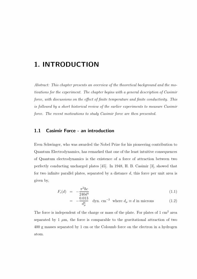
Even Schwinger, who was awarded the Nobel Prize for his pioneering contribution to
Quantum Electrodynamics, has remarked that one of the least intuitive consequences
of Quantum electrodynamics is the existence of a force of attraction between two
perfectly conducting uncharged plates [45]. In 1948, H. B. Casimir [3], showed that
for two infinite parallel plates, separated by a distance d, this force per unit area is
given by,
Fc(d) = − π2~c
240d4(1.1)
= −0.013
d4µdyn. cm−2 where dµ ≡ d in microns (1.2)
The force is independent of the charge or mass of the plate. For plates of 1 cm2 area
separated by 1 µm, the force is comparable to the gravitational attraction of two
400 g masses separated by 1 cm or the Coloumb force on the electron in a hydrogen
atom.
1. Introduction 2
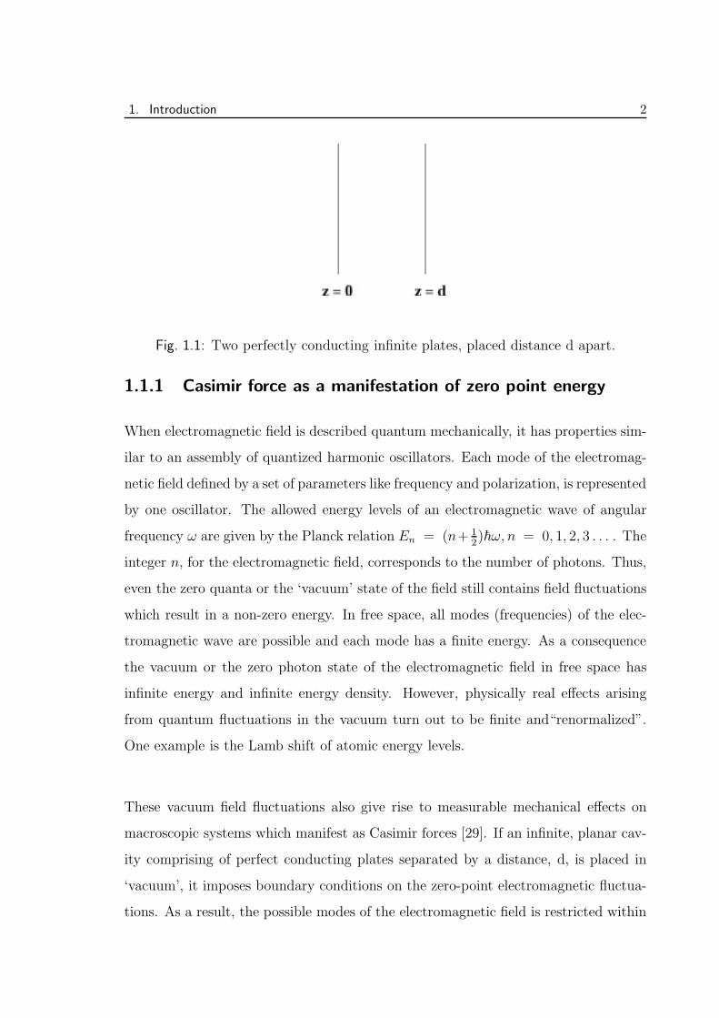
Fig. 1.1: Two perfectly conducting infinite plates, placed distance d apart.
1.1.1 Casimir force as a manifestation of zero point energy
When electromagnetic field is described quantum mechanically, it has properties sim-
ilar to an assembly of quantized harmonic oscillators. Each mode of the electromag-
netic field defined by a set of parameters like frequency and polarization, is represented
by one oscillator. The allowed energy levels of an electromagnetic wave of angular
frequency ω are given by the Planck relation En = (n+ 12)~ω, n = 0, 1, 2, 3 . . . . The
integer n, for the electromagnetic field, corresponds to the number of photons. Thus,
even the zero quanta or the ‘vacuum’ state of the field still contains field fluctuations
which result in a non-zero energy. In free space, all modes (frequencies) of the elec-
tromagnetic wave are possible and each mode has a finite energy. As a consequence
the vacuum or the zero photon state of the electromagnetic field in free space has
infinite energy and infinite energy density. However, physically real effects arising
from quantum fluctuations in the vacuum turn out to be finite and“renormalized”.
One example is the Lamb shift of atomic energy levels.
These vacuum field fluctuations also give rise to measurable mechanical effects on
macroscopic systems which manifest as Casimir forces [29]. If an infinite, planar cav-
ity comprising of perfect conducting plates separated by a distance, d, is placed in
‘vacuum’, it imposes boundary conditions on the zero-point electromagnetic fluctua-
tions. As a result, the possible modes of the electromagnetic field is restricted within
1. Introduction 3
the cavity. Thus there is a finite difference in the energy of the vacuum field outside
and inside the cavity. This results in a quantum vacuum pressure that attracts the
cavity plates together. For the zero photon state, this pressure is given by Eqn. 1.1
(see Appendix A for details).
1.1.2 Effect of Finite Temperature
The non-vacuum state of the electromagnetic field also has a Casimir force associated
with it. In general at any finite temperature, T, thermal fields are also present in
addition to the vacuum electromagnetic fields and the possible energy levels are given
by the Planck’s spectrum,
En =
(
n(ω) +1
2
)
~ω, where n(ω) =1
e~ω
kBT − 1. (1.3)
The Casimir vacuum pressure (force per unit area) is then given by [5],
F Tc (d) = − kBT
4πd3
n∑
n=0
′∫ ∞
nx
dyy2
ey − 1where x ≡ 4πkBTd/~c
† (1.4)
Fc(d) ≃ − π2~c
240d4at low T (i.e. x ≪ 1)
F Tc (d) ≃ −ζ(3)kBT
4πd3at high T (i.e. x ≫ 1) (1.5)
with ζ(3) = 1.20206 (1.6)
From these results note that the distance dependence changes from 1/d4 at low tem-
peratures to 1/d3 at high temperatures.
Considering Eqn. 1.5, it is obvious that the important non-dimensional parameter,
that distinguishes the domains of high and low temperature, is x = 4πkBTd/~c.
Moreover, it is interesting to note that high temperature also corresponds to larger
† The prime over the summation symbol means that a factor half should be inserted for the n = 0
term. See for example [5]
1. Introduction 4
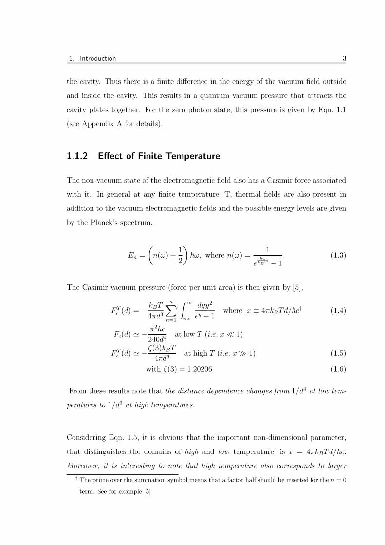
Fig. 1.2: Two semi-infinite dielectric slabs of dielectric constants ǫ1 and ǫ2, placed
distance d apart in vacuum.
separation d between the plates and vice versa. Thus at any given temperature, the
law which governs the vacuum pressure will depend on the distance between the
plates. No experiment till date has been able to observe these finite temperature
corrections to Casimir force, due to limitations in sensitivity in the distance range
where such effects start to become significant.
The primary aim of the work described in this thesis is to observe the Casimir force in
the distance range where this change in the distance dependance of the force occurs.
At a temperature of ∼ 300◦ K, the change from 1/d4 to 1/d3 is expected to occur at
about 2 µm to 4 µm. Our experiments scan separations from about 1 µm to 10 µm
and thus will be able to probe this change over from the low temperature to the high
temperature domain.
1.1.3 Effect of Finite Conductivity
The discussions so far assumed that the cavity plates are perfectly conducting, i.e,
they have infinite conductivity at all frequencies of the electromagnetic field. In
experimental situations, this simplified assumption is unrealistic and the dielectric
properties of the cavity plates should also be considered.
1. Introduction 5
Liftshitz [4] , developed the first macroscopic theory of forces between dielectrics. His
results reduce to the Casimir force given by Eqn. 1.1 for the case of perfect conductors.
For finite size plates with dielectric constants ǫ1(ω) and ǫ2(ω) [Fig. 1.2], the Casimir
force per unit area is given by the Liftshitz formula,
F pc (d) = − ~
2π2c3
∫ ∞
1
dp p2∫ ∞
0
dξ ξ3
[
{
s1 + ǫ1p
s1 − ǫ1p.s2 + ǫ2p
s2 − ǫ1p.e2ξpd/c − 1
}−1
+
{
s1 + p
s1 − p.s2 + p
s2 − p.e2ξpd/c − 1
}−1]
(1.7)
where si, p are variables that depend on the dielectric constants ǫi of the medium
and the wave vector k of the electromagnetic field. (see Appendix A for details).
1.1.4 Importance of these effects for experiments
The experiments on Casimir force are typically carried out at room temperature us-
ing metals with finite electrical conductivity. In order to make a comparison between
the experiments and the theory, it is essential to quantify the effects of temperature
and conductivity. As summarized above the effects of the thermal field fluctuations
on the Casimir force are known to become important when the spacing between the
boundaries is of the order of the characteristic length, λT = 2πωT
. ωT is the dominant
thermal angular frequency at the temperature T . Similarly, the plasma frequency ωp
of the metal determines the length scale, λp at which the finite conductivity effects
are appreciable, i.e, λp =2πωp.
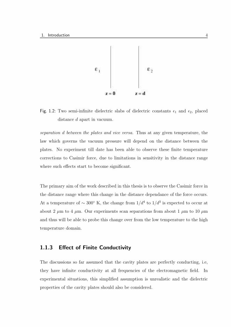
These effects have been calculated by several methods (see for example, [16, 17, 7]).
Fig. 5.2 represents one such calculation [17]. The figure shows a plot of the correction
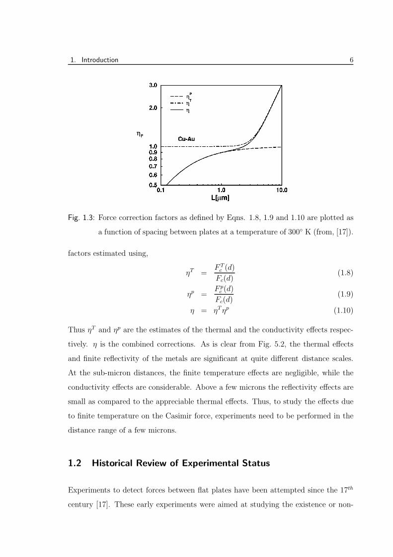
1. Introduction 6
Fig. 1.3: Force correction factors as defined by Eqns. 1.8, 1.9 and 1.10 are plotted as
a function of spacing between plates at a temperature of 300◦ K (from, [17]).
factors estimated using,
ηT =F Tc (d)
Fc(d)(1.8)
ηp =F pc (d)
Fc(d)(1.9)
η = ηTηp (1.10)
Thus ηT and ηp are the estimates of the thermal and the conductivity effects respec-
tively. η is the combined corrections. As is clear from Fig. 5.2, the thermal effects
and finite reflectivity of the metals are significant at quite different distance scales.
At the sub-micron distances, the finite temperature effects are negligible, while the
conductivity effects are considerable. Above a few microns the reflectivity effects are
small as compared to the appreciable thermal effects. Thus, to study the effects due
to finite temperature on the Casimir force, experiments need to be performed in the
distance range of a few microns.
1.2 Historical Review of Experimental Status
Experiments to detect forces between flat plates have been attempted since the 17th
century [17]. These early experiments were aimed at studying the existence or non-
1. Introduction 7
existence of the physical “vacuum”. They studied the adhesion forces between two
plates in ‘evacuated’ containers. In the 20th century, with the emergence of theories
concerning long-range, London - van der Waals interactions and Casimir force, re-
newed experiments were carried out. (For a review of the experiments until 2001,
see [4])
The earliest attempt to measure Casimir force was by Overbeek and Sparnaay [15] in
1952. They tried to measure the force between two parallel polished flat glass plates
with a surface area of 1 cm2, in the distance range of 0.6 µm to 1.5 µm. The mea-
surements at 1.2 µm, ‘pointed to the existence of a force which was of the expected
order of magnitude’ [17].
Derjaguin and Abrikossova [8, 7] were the first to obtain results in the distance range
0.1 µm - 1.0 µm that were in agreement with Lifshitz’s theory. Sparnaay [16] re-
peated his measurements with metal plates in 1957. He measured the force between
chromium plates and chromium-steel plates. The measurements did not ‘contradict’
the expected force per unit area from Casimir’s relation.
The next major set of improved measurements with metallic surfaces were performed
by van Blokland and Overbeek [18] nearly 20 years later, in 1978. They measured the
forces between a lens and a flat plate coated with chromium using a spring balance
at distances between 0.13 µm and 0.67 µm. This measurement can be considered as
the first unambiguous demonstration of the Casimir force between metallic surfaces.
In the last decade, attempts to understand the nature of quantum fluctuations at
macroscopic scales and predictions of new long range forces at the sub-millimeter
scales by theories that unify the fundamental forces have rekindled interest in Casimir
force measurements. The earliest of these was by Lamoreaux in 1997 [24], who mea-
sured the Casimir force between a lens and a plate using a torsion balance in the range
1. Introduction 8
0.6 µm - 6 µm. In a later experiment, Mohideen et al. [14] measured the Casimir
force for separations from 0.1 µm to 0.9 µm using an atomic force microscope. Ex-
periments at Bell-Labs by Chan et al. [4] indicate that Casimir type forces play an
important role in micro-electromechanical systems. Recently Bressi et al. [2] have
carried out high precision experiments between parallel plates in the range 0.5 µm -
3 µm and the related force coefficient was determined at the 15% precision level. The
most recent experiment by Decaa et. al. measures the Casimir force between two
dissimilar metals for separations of 0.2 µm - 2 µm.
A more detailed review and a discussion of data from the recent experiments on
Casimir force will be presented in a later chapter. All the experiments performed so
far to measure Casimir force were carried out at room temperatures and probed the
distance range of 0.1 µm to 3 µm. As the separation increases, the force decreases
rapidly as d−4 to start with and as d−3 in the finite temperature regime [Eqn. 1.5]. It
is important to measure the force at d > 3 µm to detect and characterize the finite
temperature corrections to the Casimir force.
1.3 Motivations to study Casimir force
Historically Casimir derived his results while attempting to explain the inter-molecular
interactions seen in experiments on colloidal suspensions. Casimir force was looked
upon as the effect of finite speed of light (retardation effect) on the London - van
der Waals interaction. The early experiments that measured the force of attraction
between surfaces where aimed at understanding the inter atom interactions and to
see the change over from the van der Waals force at very small separations to the
retarded van der Waals or Casimir force as the separations increased. The interest
slowly waned once the macroscopic theories of interactions were verified by experi-
ments.
In modern times, interest in Casimir force has been aroused by the crucial role it plays
1. Introduction 9
in theories of fundamental physics. Casimir force provides explicit evidence for the
existence of vacuum fluctuations and for the interplay between the microscopic (quan-
tum) and the macroscopic worlds. Also, in the last couple of decades, several new
theories have been proposed that predict new physics in the sub-millimeter distance
range. Casimir force is the dominant background in this range and hence it becomes
essential to understand all aspects of Casimir force before looking for new forces at
these scales.
1.3.1 Understanding the Quantum Vacuum
The existences of electromagnetic field fluctuations in vacuum presents problems due
to the amount of energy it carries. General Relativity states that all forms of mat-
ter and energy should gravitate. The large energy density, ρv associated with the
vacuum fluctuations should induce very large gravitational effects, much larger than
that allowed by observations. This “vacuum catastrophe” is related to the famous
cosmological constant problem (see [51, 52, 44, 40] for a review).
In 1917, when Einstein first attempted to apply his new theory to relativity to the
Universe, the Universe was believed to be static. Einstein could not construct a static
universe if there was only matter and curvature, so he introduced a free parameter Λ,
the cosmological constant, into his theory which was a form of energy with negative
pressure. With the discovery of the expansion of the Universe, Einstein suggested
that this could be dropped. But it was retained alive in discussions of cosmology,
and has been used time and again to explain observations that did not fit into the
standard scenarios in cosmology [10, 48]. Currently, there is strong observational
evidence [43, 41] for an accelerated expansion of the Universe. This can be explained
by a non-vanishing cosmological constant. Thus, in the present scenario, the geometry
of the Universe is determined by the energy density of matter, ρm, the energy density
due to vacuum, ρv and that from the cosmological constant, Λ/(8πG). The quantum
vacuum has properties similar to those attributed to a positive cosmological constant,
1. Introduction 10
the most important property being an effective repulsive gravity. This is because
the acceleration is proportional, in General Relativity, to the term −(ρ + 3p) of
the matter, where ρ is the energy density and p the pressure. For normal matter,
the term (ρ + 3p) is positive and therefore, the universe is expected to decelerate
as it expands. The diagonal elements of the energy momentum tensor are energy
density and the three components of pressure. Therefore, an energy momentum
tensor that is proportional to “vacuum” with diagonal elements (1,−1,−1,−1) will
have its equation of state ρ = −p, and the effective acceleration of the Universe
with such a source term will be positive. It is this property that allowed Einstein to
construct a static Universe, balancing the gravitational attraction of normal matter
with the effective repulsion of the cosmological constant. The total energy density in
the Universe, ρc can be determined from the expansion rate of the Universe and is
given by 3H20/(8πG), where H0 is the Hubble constant. Cosmological data indicates
that ρv = 0.7 ρc ∼ 4 keV/cm3. A naive estimate of ρv calculated for all modes of
the zero point field with a high frequency cut-off at the Planck scale is 120 orders of
magnitude larger than ρc. Therefore, there is a need to find a fine-tuned suppression
mechanism that will bring this large number close to zero. If a small vacuum energy as
well as a cosmological constant are present, then their values need to be fine tuned to
the small number ρc, which amounts to a fine cancelation to 120 decimal places. This
bizarre coincidence is the present cosmological constant problem. To find a solution
to this problem, the contributions from the vacuum fields have to be understood
and estimated better. Since Casimir force is a direct manifestation of the vacuum
fluctuations, it provides a tool to comprehend the ‘vacuum’.
1.3.2 “The Hierarchy Problem”
Interactions in nature have been identified to be of four fundamental type: gravita-
tional, electromagnetic, strong and weak. General Theory of relativity and Standard
Model of particles physics are the two most successful theories that explain these in-
teractions. Attempts to link these two theories are plagued with difficulties due to the
1. Introduction 11
vast differences in the strength of gravity as compared to others. The Standard Model
of electroweak and strong interactions unifies electromagnetic and weak interactions
at the characteristic energy scale, Mew of 103 GeV (= 1 TeV). The energy scale of
gravity is the Planck energy, Mpl (= 1019 GeV), where the Compton wavelength of
a particle becomes equal to its Schwarzchild radius. In natural units (~ = c = 1),
the gravitational constant G = 1/M2pl. The vast difference between these two en-
ergy scales is the “hierarchy problem”. Several frameworks have been put forward to
solve this problem. The most popular among them are string theories, M-theory and
theories with large extra dimensions (see [1] for a recent review).
Large extra dimensions and Warped geometries
A model that attempts to reconcile gravity and quantum theory is one in which the
fundamental objects that constitute our Universe are not particles but very tiny ex-
tended objects: strings. However, to have a consistent string theory that can explain
all known phenomena, spatial dimensions larger than 3 are required (for a review, see
[42, 4, 1]). The question then is, why do we not see these additional dimensions?
Two scenarios have been proposed to explain this. One that follows the original idea
by Kaluza [32], which tries to unify the fundamental forces at Planck scale. In this
picture, besides the three spatial dimensions of infinite extent, there are additional
dimensions of finite size, rc, that are curled up as compactified circular extra di-
mensions. The typical size of the circle would be determined by the Planck length,
10−33cm. This means that physics at short distances appears to be higher dimensional
and forces go as 1/r−(n+2), where n is the number of extra dimensions. At distances
much larger than rc, n = 0 and one observes the 1/r2 law. Around the compatifica-
tion scale, the forces can be modelled as e−r/rc and would show up as deviations from
the standard law.
The other idea proposed by Arkani-Hamed and others [5, 3] , tries to unify forces at
1. Introduction 12
the TeV scale, thereby removing the hierarchy problem. The 1032 times weakness of
gravity as compared to the other forces at this electroweak scale is explained by the
presence of the extra-dimensions of finite size R∗. They propose that the three spatial
dimensions in which we live are perhaps just a membrane (3-brane) embedded in a
higher dimensional bulk of (3+n) spatial dimensions. The Standard Model fields are
confined to the 3-brane while gravity can propagate into the bulk. Thus, at distances
greater than R∗, gravity spreads in all 3+n dimensions and goes as 1/r−(n+2) while the
strength of the other forces, still falls as 1/r2. At r > R∗, gravity too reverts back to
1/r2. This scenario is distinguished by the term, “large extra dimensions scenario”, as
the additional dimensions in this theory could even be macroscopic. If there were only
one extra dimension, its size would have to be of the order of 1010 km to account for
the weakness of gravity. Such an extra dimension would change the dynamics of the
Solar system and is eliminated by known experimental results. With two equal extra
dimensions, the scale length would be of the order of a 0.3 mm. This is inconsistent
with laboratory experiments [22] and astrophysical bounds [2, 12, 20, 21]. For n ≥ 3,
the scale length is less than about a nanometer. This does not imply that the new
dimensions will not show observable effects in experiments at sub-millimeter scales.
A single large dimension of size 1 mm with several much smaller extra dimensions
is still allowed. Experiments have shown that the scale length of the ‘largest’ extra
dimension has to be < 200 µm [22, 1]. This would give rise to observable changes
to inverse square law of gravity at these scales. At such distances, the strengths of
gravity and Casimir forces are comparable and in order to look for new corrections
to inverse square law of gravity, Casimir background has to be first understood and
eliminated.
New particles
The super-symmetric extensions to standard model unify the electro-weak and strong
interactions at energy scales of 1016 GeV, which is very close to the Planck scale,
1. Introduction 13
with the additional assumption that there are no charged particles between the TeV
and the Planck scale (see for ex. [4, 42] and references therein). A trade mark of
super-string theories is the occurrence of scalar partners of the graviton (dilaton),
gravitationally coupled massless scalers called moduli, and other light scalers like ax-
ions. The exchange of these particles could give rise to Yukawa type interactions, that
would appear in experiments that measure forces. The range λ, of these interactions
depends on the mass of the elementary particle. For super-symmetric theories with
low energy (few TeV) symmetry breaking, these scalar particles would produce effects
in the sub-millimeter scales [23, 30]. The predictions on the strength of these effects
is less precise than those of the extra-dimension scenarios.
-8 -7 -6 -5
0
5
10
15
20
25
6
7,a7,b
89
10
11
12
13 log(�=1m)
log j�Gj
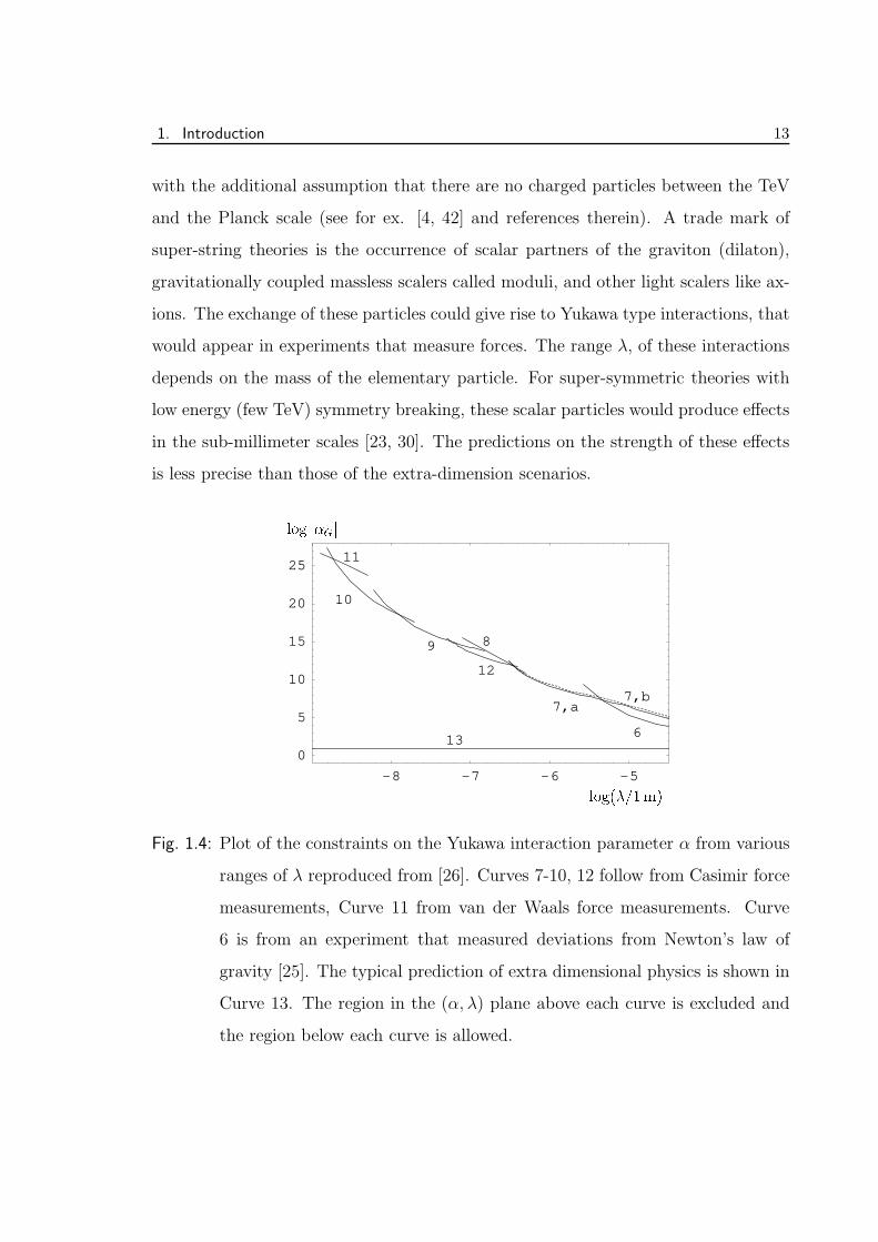
Fig. 1.4: Plot of the constraints on the Yukawa interaction parameter α from various
ranges of λ reproduced from [26]. Curves 7-10, 12 follow from Casimir force
measurements, Curve 11 from van der Waals force measurements. Curve
6 is from an experiment that measured deviations from Newton’s law of
gravity [25]. The typical prediction of extra dimensional physics is shown in
Curve 13. The region in the (α, λ) plane above each curve is excluded and
the region below each curve is allowed.
References 14
1.3.3 Constraints on new macroscopic forces
Keeping in mind that the strengths of the new macroscopic forces are small, their
potentials are scaled with respect to the gravitational interaction between two point
masses as shown below:
V (r) = −GM1M2
r
(
1 + αe−rλ
)
(1.11)
where α represents the coupling strength of the interaction and λ the range [23, 27].
The typical scale of λ will vary depending on the source of the potential. For the
extra dimension scenarios it would be the size of the extra dimension, while for the
new string inspired forces, it would be proportional to the inverse of the mass of the
mediating particle. Thus constraints can be placed on the parameter space of α− λ
from experiments that study long-range interactions [5]-[11]. For distances of . 0.1
mm, Casimir force provides the dominant background and best limits on α for these
λ can be obtained from Casimir force measurements. The available constraints to
date on α− λ from various experiments are summarised in Fig.1.4.
The torsion balance experiments described in this thesis are capable of strongly
constraining theories with macroscopic extra dimensions, apart from measuring the
Casimir force and its finite temperature corrections.
References
[1] E. G. Adelberger. Sub-millimeter Tests of the Gravitational Inverse Square Law.
http://arXiv.org/abs, hep-ex/0202008, 2002.
[2] E. G. Adelberger, Heckel, and Nelson A. E. B. R. Tests of the Gravitational
Inverse sqare law. Ann. Rev. of Nuclear and Particle Science, 53:77, December
2003.
[3] I. Antoniadis, N. Arkani-Hamed, S. Dimopoulos, and G. Dvali. New Dimension
at a Millimeter to a Fermi and Superstrings at a TeV. Phys. Lett. B, 436:257,
1998.
References 15
[4] N. Arkani-Hamed. Large Extra Dimensions: A new Arena for Particle Physics.
Physics Today, page 35, Feb. 2002.
[5] N. Arkani-Hamed, S. Dimopoulos, and G. Dvali. The Hierarchy Problem and
New Dimension at a Millimeter. Phys. Lett. B, 429:268, 1998.
[6] N. Arkani-Hamed, S. Dimopoulos, and G. Dvali. Phenomenology, astrophysics,
and cosmology of theories with submillimeter dimensions and TeV scale quantum
gravity. Phys. Rev. D, 59:086004, April 1999.
[7] M. Bordag, B. Geyer, G. L. Klimchitskaya, and V. M. Mostepanenko. Casimir
Force at Both Nonzero Temperature and Finite Conductivity. Physical Review
Letters, 85:503–506, July 2000.
[8] M. Bordag, U. Mohideen, and V. M. Mostepanenko. New Developements in
Casimir Force. Phys. Rep., 353:1, 2001.
[9] G. Bressi et al. Measurement of the Casimir Force between Parallel Metallic
Surfaces. Phys. Rev. Lett, 88:041804–1, 2002.
[10] R. R Caldwell and P J Steinhardt. Quintessence. Physics Worlds, page 31, Nov
2000.
[11] H. B. Casimir. On the Attraction Between Two Perfectly Conducting Plates.
Proc. K. Ned. Akad. Wet., 51:793, 1948.
[12] H. B. Chan et al. Quantum Mechanical Actuation of Micromechanical Systems
by the Casimir Force. Science, 291:9, 2001.
[13] R Cowsik. A new torsion balance for studies in gravitation and cosmology. Indian
Journal of Physics, 55B:487, 1981.
[14] R Cowsik. Challenges in experimental gravitation and cosmology. Technical
report, Dept. of Science & Technology, New Delhi, 1982.
[15] R Cowsik. Search for new forces in nature. In From Mantle to Meteorites (Prof.
D.Lal Festschrift), 1990.
References 16
[16] R. Cowsik, N. Krishnan, P. Sarawat, S. N Tandon, and S. Unnikrishnan. The
Fifth Force Experiment at the TIFR. In Gravitational Measurements, Funda-
mental Metrology and Constants, 1988.
[17] R. Cowsik, N. Krishnan, P. Sarawat, S. N Tandon, and S. Unnikrishnan. Limits
on the strength of the fifth-force. In Advances in Space Research (Proc. XXI
COSPAR, Espoo), 1989.
[18] R. Cowsik, N. Krishnan, S. N. Tandon, and C. S. Unnikrishnan. Limit on the
strength of intermediate-range forces coupling to isospin. Physical Review Letters,
61:2179–2181, November 1988.
[19] R. Cowsik, S. N Tandon, and N. Krishnan. Sensitive test of Equivalence Princi-
ple. Technical report, Dept. of Science & Technology, New Delhi, 1982.
[20] S. Cullen and M. Perelstein. SN 1987A Constraints on Large Compact Dimen-
sions. Physical Review Letters, 83:268–271, July 1999.
[21] B. V Derjaguin. The Force Between Molecules. Sci. Am., 203:47, 1960.
[22] B. V Derjaguin and J. J. Abrikossova. Disc. Faraday Soc., 18:33, 1954.
[23] S. Dimopoulos and G. F. Giudice. Macroscopic Forces from Supersymmetry.
Phys. Lett. B, 379:105, 1996.
[24] C. Genet. La Force de Casimir Entre Deux Miroirs Metalliques A temperature
Non Nulle. PhD thesis, Laboratoire Kastler Brossel, University of Paris, Paris,
Italy, 1999.
[25] C. Genet, A. Lambrecht, and S. Reynaud. Temperature dependence of the
Casimir effect between metallic mirrors. Phy.Rev. A, 62:012110, July 2000.
[26] C. Hanhart, D. R. Phillips, S. Reddy, and M. Savage. Extra dimensions,
SN1987a, and nucleon-nucleon scattering data. Nuclear Physics B, 595:335–359,
February 2001.
References 17
[27] C. Hanhart, J. A. Pons, D. R. Phillips, and S. Reddy. The likelihood of GODs’
existence: improving the SN 1987a constraint on the size of large compact di-
mensions. Physics Letters B, 509:1–2, June 2001.
[28] C. D. Hoyle, U. Schmidt, B. R. Heckel, E. G. Adelberger, J. H. Gundlach, D. J.
Kapner, and H. E. Swanson. Submillimeter Test of the Gravitational Inverse-
Square Law: A Search for “Large” Extra Dimensions. Physical Review Letters,
86:1418–1421, February 2001.
[29] M. Jaekel, A. Lambrecht, and S. Reynaud. Quantum vacuum, inertia and grav-
itation. New Astronomy Review, 46:727–739, November 2002.
[30] D. B. Kaplan and M. B. Wise. Coupling of the light Dialoton and Violations of
the Equivalance Principle. J. High Energy Phys., 08:37, 2000.
[31] N. Krishnan. Search for Intermidiate Range forces Weaker than Gravity. PhD
thesis, Tata Institute of Fundamental Research, Mumbai, India, 1989.
[32] T. Kulza. Preuss. Akad. Wiss., page 966, 1921.
[33] S. K. Lamoreaux. Demonstration of the Casimir Force in the 0.6 to 6 µ Range.
Phys. Rev. Lett, 78:5, 1997.
[34] E. M. Lifshitz. Theory of molecular attraction between solids. Sov. Phys. JETP,
2:73, 1956.
[35] J. C. Long et al. Upper Limit on Submillimeter-range Forces from Extra Space-
time dimensions. Nature, 421:924, 2003.
[36] W. P Milonni. The Quantum Vacuum: An Introduction to Quantum Electrody-
namics. Academic Press, Newyork, 1994.
[37] U. Mohideen and A Roy. Precision Measurement of the Casimir Force from 0.1
to 0.9 µm Range. Phys. Rev. Lett, 81:4549, 1998.
References 18
[38] V. M. Mostepanenko. Constraints on Non-Newtonian Gravity from Recent
Casimir Force Measurements. ArXiv General Relativity and Quantum Cosmology
e-prints, November 2003.
[39] J. T. G. Overbeek and M. J. Sparnaay. Proc. K. Ned. Akad. Wet., 54:387, 1952.
[40] T. Padmanabhan. Cosmological constant-the weight of the vacuum. Phys. Rep.,
380:235–320, July 2003.
[41] S. Perlmutter et al. Measurements of Omega and Lambda from 42 High-Redshift
Supernovae. Astrophys. J, 517:565–586, June 1999.
[42] L. Randall. Extra Dimensions and Warped Geometries. Science, 296:1422, 2002.
[43] A. G. Riess et al. Observational Evidence from Supernovae for an Accelerating
Universe and a Cosmological Constant. Astron. J, 116:1009–1038, September
1998.
[44] V. Sahni. The cosmological constant problem and quintessence. Classical and
Quantum Gravity, 19:3435–3448, July 2002.
[45] J. Schwinger, L. L. DeRaad, Jr., and K. A. Milton. Casimir Effect in Dielectrics.
Ann. Phys. NY, 115:1, 1978.
[46] M. J. Sparnaay. Attractive Forces Between Flat Plates. Nature, 180:334, 1957.
[47] M. J. Sparnaay. Historical Background of Casimir force. In A. Sarlemijn and
M. J. Sparnaay, editors, Physics in the Making, North-Holland, 1989. Elsevier
Science Publishers B V.
[48] N. Straumann. The History of the Cosmological COnstant Problem. ArXiv
General Relativity and Quantum Cosmology e-prints, August 2008.
[49] C. S. Unnikrishnan. Torsion Balance Experiments to Search for New Composition
Dependant Forces. PhD thesis, Tata Institute of Fundamental Research, Mumbai,
India, 1992.
References 19
[50] P. H. G. M van Blokland and J. T. G. Overbeek. van der Waals Forces Be-
tween Objects Covered with Chromium Layer. J. Chem. Soc. Faraday Trans.
72, 72:2637, 1978.
[51] S. Weinberg. The cosmological constant problem. Reviews of Modern Physics,
61:1–23, January 1989.
[52] S. Weinberg. The Cosmological Constant Problems. In Sources and Detection
of Dark Matter and Dark Energy in the Universe, page 18, 2001.
2. TORSION BALANCE- DESIGN AND
FABRICATION
Abstract: This chapter is devoted to the description of the main components of the
experimental set up. An overview of the experimental scheme will be followed by a
detailed explanation of the various components of the experiment. The procedures
followed during assembly to reduce systematic and environmental noises will be de-
scribed.
2.1 General principle of the apparatus
Torsion pendulums have been used as transducers for precision measurements for
over two centuries. They are known for their capability to isolate and measure feeble
effects that would otherwise be difficult if not impossible to observe against the back-
ground gravitational field of the earth.(see for ex., [3, 1]) Our experimental set up is
aimed at achieving the sensitivity required to measure the finite temperature effect
in the Casimir force using a torsion pendulum, optical auto-collimator combination.
[2, 4]. The experiment was to be performed in the separation range 2 µm - 10 µm.
Casimir force at 10 µm will produce, in static case, a deflection of ∼ 10−6 radians on
our pendulum. This is well with in the sensitivity of ∼ 10−8 radians of our optical
lever.
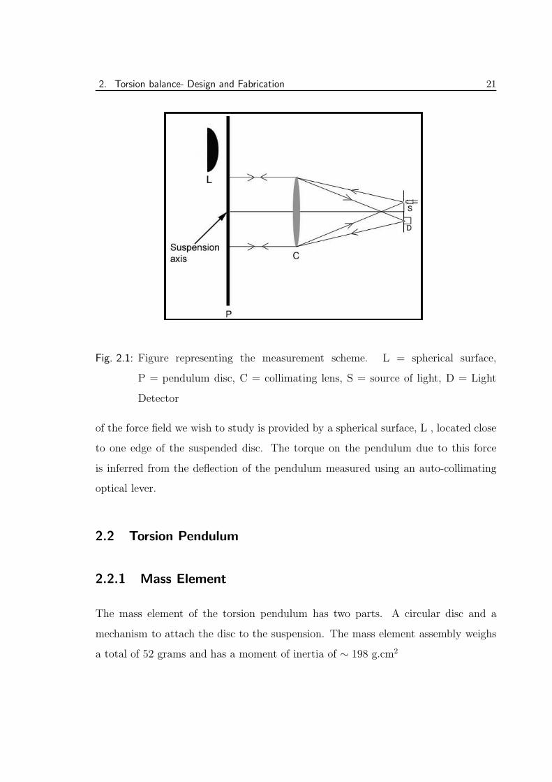
The measurement scheme [Fig. 2.1] broadly consists of a torsional pendulum with a
flat circular disc, P , as mass element, suspended using a thin strip fibre. The source
2. Torsion balance- Design and Fabrication 21
Fig. 2.1: Figure representing the measurement scheme. L = spherical surface,
P = pendulum disc, C = collimating lens, S = source of light, D = Light
Detector
of the force field we wish to study is provided by a spherical surface, L , located close
to one edge of the suspended disc. The torque on the pendulum due to this force
is inferred from the deflection of the pendulum measured using an auto-collimating
optical lever.
2.2 Torsion Pendulum
2.2.1 Mass Element
The mass element of the torsion pendulum has two parts. A circular disc and a
mechanism to attach the disc to the suspension. The mass element assembly weighs
a total of 52 grams and has a moment of inertia of ∼ 198 g.cm2
2. Torsion balance- Design and Fabrication 22
The Disc:
The active element of the suspension is a circular disc of thickness 4 mm and diameter
80 mm made of glass. The edges of the disc are chamfered and both the faces are
polished to have a surface finish of λ/2 and are coated with a 1 µm thick layer of
gold. One of the faces acts as a conducting boundary for the force under study and
the other face acts as a mirror viewed by a sensitive optical lever which measures the
angle that the normal to the disc makes with the optic axis of the optical lever.
The Disc holder:
The gold coated glass disc is held in a frame made of a gold strip that is 80 µm
thick and 4 mm wide. In order to hold the glass disc firmly, this strip is shaped
to form a groove that matches the chamfered edges of the disc and forms a circular
frame around the disc. The ends of this strip are held securely between the flat
surfaces of an Aluminium holder [Fig. 2.2]. The flat surfaces that press the strip ends
together have 50 µm deep, 4mm wide channels machined with the central axis of the
channel along the axis of the holder. These locate the strip and hence the pendulum
bob along the axis of the holder. The top of this holder has a 2 mm diameter hole
through its central axis to hold the torsional fibre. This holder is also gold coated to
avoid aluminium oxide layers that can accumulate charges.
2.2.2 The Pendulum Suspension
The mass element is suspended in two stages to avoid non-torsional modes of oscilla-
tion of the pendulum. The suspension consists of a pre-suspension, a device to damp
the simple pendular modes of the fibre, and the main suspension.
2. Torsion balance- Design and Fabrication 23
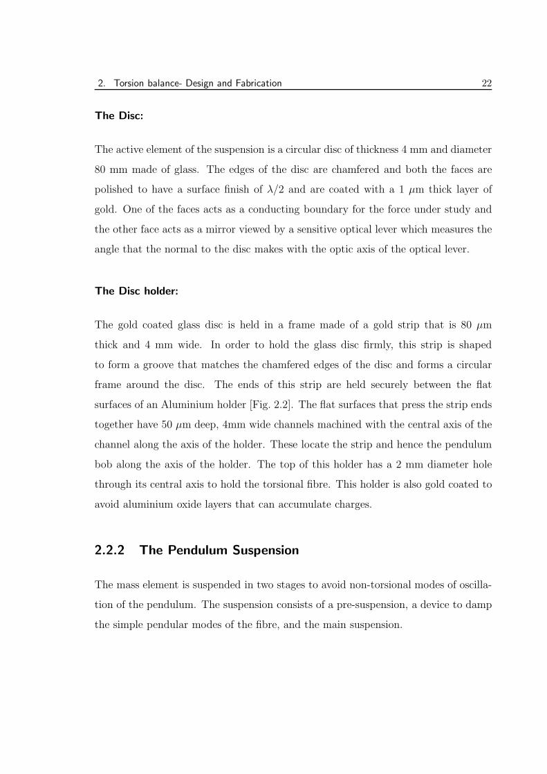
Fig. 2.2: Picture of Mass element assembly. A = Aluminium holder, P = Pendulum
Disc
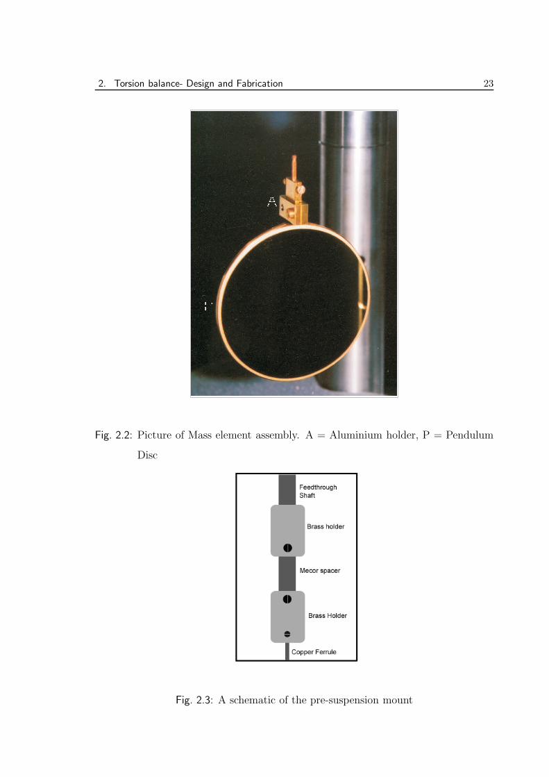
Fig. 2.3: A schematic of the pre-suspension mount
2. Torsion balance- Design and Fabrication 24
Pre-suspension:
The first portion of the suspension is a torsionally stiff copper wire of 100 µm diameter.
This ensures verticality of the main suspension that uses a metal ribbon. The pre-
suspension is essential to avoid spurious torsional effects due to tilts of the suspensions.
The ends of the stiff wire are passed through a copper ferrule of outer diameter 2 mm
and bore diameter of about 0.5 mm. The ferrule is crimped such that it holds the
fibre gently but firmly along its central axis. The length of the Copper wire is 7 cm
between the ferrules. The wire is mounted from the shaft of a rotary feed-through that
is attached to the top of the vacuum chamber housing the experiment. To electrically
isolate the suspension from the chamber, the wire is held through a Macor insulator
as described below [Fig. 2.3]. The shaft holds a cylindrical clamp made of brass,
which in turn holds a Macor cylinder. Another cylindrical brass holder is mounted to
this Macor piece and has a 2 mm diameter hole along its axis. The ferrule at one end
of the wire is passed through this hole and held in place by a screw. A copper disc
is suspended from the ferrule at the other end of the wire using a similar mechanism
[Fig. 2.4]. Kapton insulated copper wires connect the fibre suspension to an electrical
feed-through mounted on the vacuum chamber.
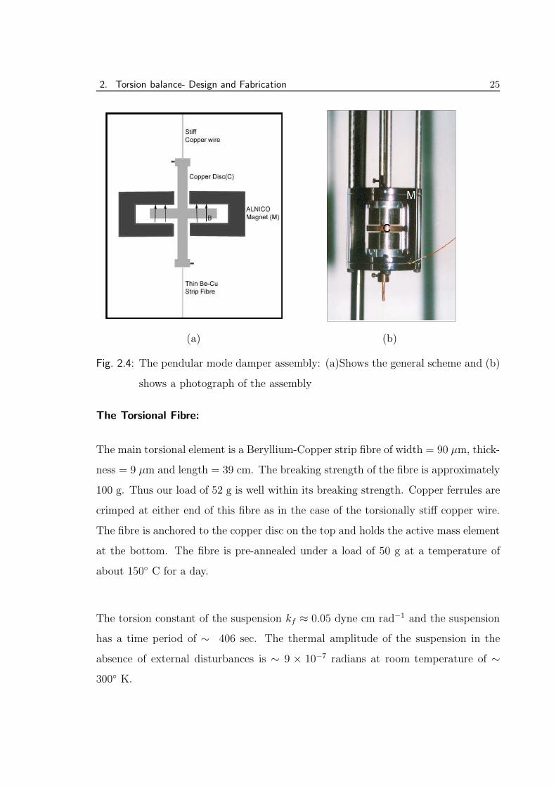
Pendular Mode Damper:
The copper disc (C) passes between the pole pieces of an aluminium-nickel-cobalt
ring magnets (M) [Fig. 2.4] such that it cuts across the field lines (B) of the magnet.
The fast pendular oscillations of the fibre and violin modes cause eddy currents to
flow in the copper disc and dissipate these modes. Thus, these modes will be damped
out rapidly. Since the copper disc and the magnet are axially symmetric, the very
slow torsional modes are not damped.
2. Torsion balance- Design and Fabrication 25
(a) (b)
Fig. 2.4: The pendular mode damper assembly: (a)Shows the general scheme and (b)
shows a photograph of the assembly
The Torsional Fibre:
The main torsional element is a Beryllium-Copper strip fibre of width = 90 µm, thick-
ness = 9 µm and length = 39 cm. The breaking strength of the fibre is approximately
100 g. Thus our load of 52 g is well within its breaking strength. Copper ferrules are
crimped at either end of this fibre as in the case of the torsionally stiff copper wire.
The fibre is anchored to the copper disc on the top and holds the active mass element
at the bottom. The fibre is pre-annealed under a load of 50 g at a temperature of
about 150◦ C for a day.
The torsion constant of the suspension kf ≈ 0.05 dyne cm rad−1 and the suspension
has a time period of ∼ 406 sec. The thermal amplitude of the suspension in the
absence of external disturbances is ∼ 9 × 10⁻⁷ radians at room temperature of ∼300◦ K.
2. Torsion balance- Design and Fabrication 26
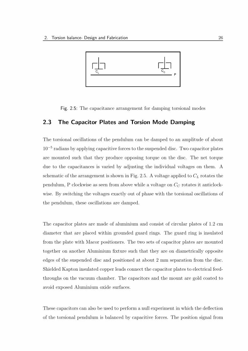
Fig. 2.5: The capacitance arrangement for damping torsional modes
2.3 The Capacitor Plates and Torsion Mode Damping
The torsional oscillations of the pendulum can be damped to an amplitude of about
10−5 radians by applying capacitive forces to the suspended disc. Two capacitor plates
are mounted such that they produce opposing torque on the disc. The net torque
due to the capacitances is varied by adjusting the individual voltages on them. A
schematic of the arrangement is shown in Fig. 2.5. A voltage applied to CL rotates the
pendulum, P clockwise as seen from above while a voltage on CC rotates it anticlock-
wise. By switching the voltages exactly out of phase with the torsional oscillations of
the pendulum, these oscillations are damped.
The capacitor plates are made of aluminium and consist of circular plates of 1.2 cm
diameter that are placed within grounded guard rings. The guard ring is insulated
from the plate with Macor positioners. The two sets of capacitor plates are mounted
together on another Aluminium fixture such that they are on diametrically opposite
edges of the suspended disc and positioned at about 2 mm separation from the disc.
Shielded Kapton insulated copper leads connect the capacitor plates to electrical feed-
throughs on the vacuum chamber. The capacitors and the mount are gold coated to
avoid exposed Aluminium oxide surfaces.
These capacitors can also be used to perform a null experiment in which the deflection
of the torsional pendulum is balanced by capacitive forces. The position signal from
2. Torsion balance- Design and Fabrication 27
the optical lever is fed back to control the effective voltage on the capacitor plates
and the torsion pendulum ‘locked’ at a fixed position. If the torque on the pendulum
due to force between the pendulum and the spherical lens surface is modified, voltage
on the capacitors changes to balance this torque. Thus, the change in voltage on the
capacitor is a direct signal of the torque acting on the pendulum.
The varying voltages are generated from a 16 bit DAC in a PCI interface card.
Typically one volt on the capacitor at 1 mm separation, gives rise to a torque of
∼ 10−3 dyne.cm. The voltage on one capacitor is kept fixed at about 4 V and that on
the other is varied from 0 V - 10 V so that both positive and negative torques may be
applied to the pendulum. The information on the angular position of the suspended
disc obtained from the autocollimator is fed back to a PID loop through software
(Labview) to control the voltage of the capacitor. When the lens is far away and the
only force on the suspension is the restoring force from the fibre, the PID loop keeps
the position of the pendulum locked to about 1/10 of a pixel or 5 × 10⁻⁷ radians (1
sec integration). This is below the thermal amplitude of the pendulum which is of
the order of 10−6 radians.
2.4 The Spherical Lens and the Compensating Plate
In our experiment the Casimir force between the suspended disc and the spherical
surface of a lens is measured. This configuration is simpler to implement as difficulties
in holding the 2 plates parallel to each other while measuring the force are avoided.
The lens is 25 mm in diameter and has a radius of curvature of about 38 cm. It
is coated with 1 µm thick layer of gold. It is mounted in a cell and held along the
diameter of the suspended disc close to one edge such that the interactions between
the lens and the mass element apply a torque on the pendulum. In this position,
the gravity due to the lens cell assembly will also apply a torque on the suspension.
This is minimized by using a compensating plate of Aluminium with mass equal to
2. Torsion balance- Design and Fabrication 28
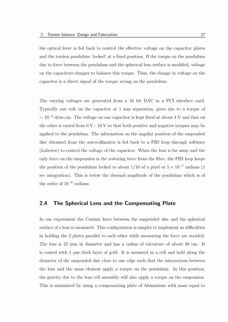
Fig. 2.6: The lens (L), compensating plate (C) and the capacitor plates (CL and Cc)
assembled (without the pendulum). T is the translation stage and E the
EncoderMiker
that of lens and the cell [Fig. 2.6]. The outer diameter of the compensating plate is
equal to that of the lens cell, but the compensating plate has a flat surface facing
the suspended disc and its thickness is adjusted to equalize the masses. The compen-
sating plate is mounted such that the gravitational torque due to the plate opposes
the gravity due to the lens assembly. The net gravitational torque on the pendulum
is small. More importantly, changes in the force as the lens is moved through small
distances is negligible compared to the changes in Casimir force and electrostatics
forces. The lens assembly and the compensating plate are together mounted on a
translation stage (T) (Newport Model- 461 series)(Fig. 2.6). An EncoderMiker ac-
tuator (E) from Oriel is used to translate this stage perpendicular to the disc surface.
The actuator movement is controlled by DC voltages applied to it. The encoder has
a resolution of 0.05 µm and its output is monitored using a Data acquisition card
with a PCI interface attached to the PC.
The lens assembly and the compensating plate are electrically isolated from each
other and from the mount. Kapton insulated copper wires connect them to separate
2. Torsion balance- Design and Fabrication 29
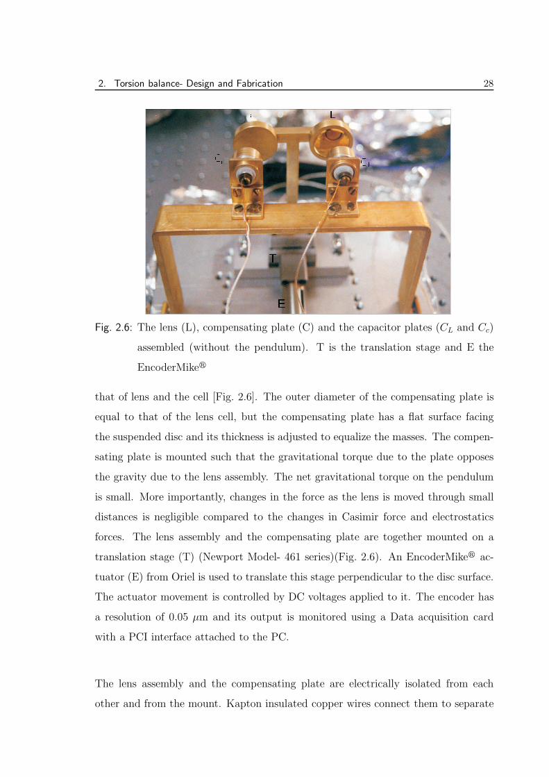
Fig. 2.7: Picture of the torsion pendulum, capacitors and the lens assembled inside
the vacuum chamber
connectors on an electrical feed-through attached to the vacuum chamber.
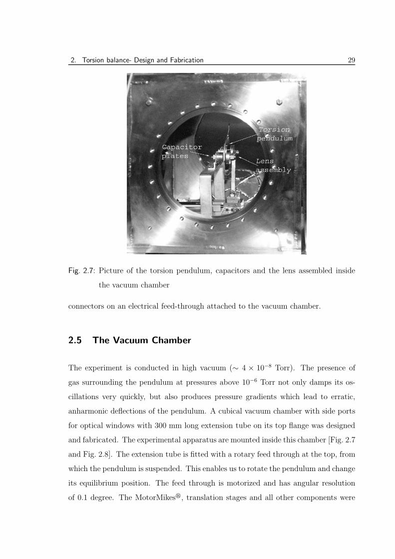
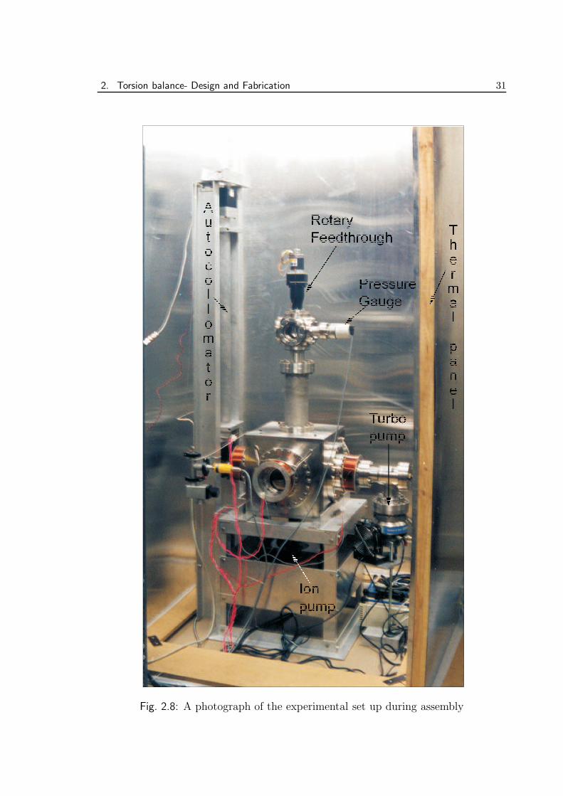
2.5 The Vacuum Chamber
The experiment is conducted in high vacuum (∼ 4 × 10⁻⁸ Torr). The presence of
gas surrounding the pendulum at pressures above 10−6 Torr not only damps its os-
cillations very quickly, but also produces pressure gradients which lead to erratic,
anharmonic deflections of the pendulum. A cubical vacuum chamber with side ports
for optical windows with 300 mm long extension tube on its top flange was designed
and fabricated. The experimental apparatus are mounted inside this chamber [Fig. 2.7
and Fig. 2.8]. The extension tube is fitted with a rotary feed through at the top, from
which the pendulum is suspended. This enables us to rotate the pendulum and change
its equilibrium position. The feed through is motorized and has angular resolution
of 0.1 degree. The MotorMikesr, translation stages and all other components were
2. Torsion balance- Design and Fabrication 30
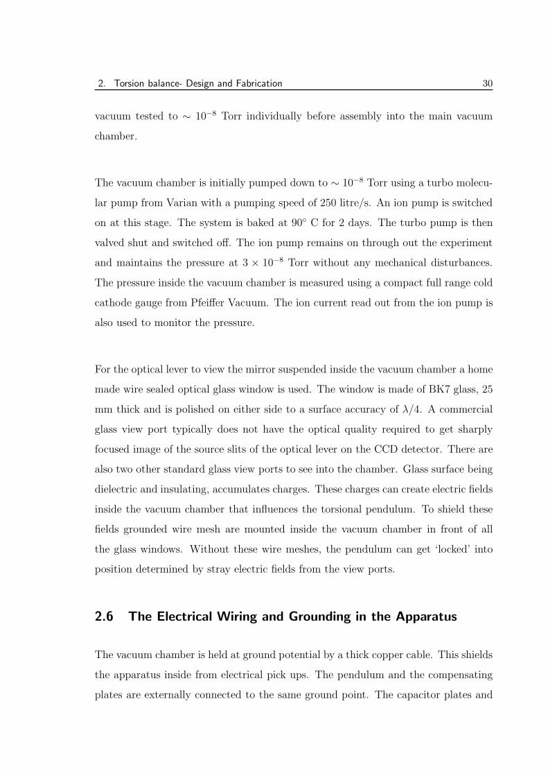
vacuum tested to ∼ 10−8 Torr individually before assembly into the main vacuum
chamber.
The vacuum chamber is initially pumped down to ∼ 10−8 Torr using a turbo molecu-
lar pump from Varian with a pumping speed of 250 litre/s. An ion pump is switched
on at this stage. The system is baked at 90◦ C for 2 days. The turbo pump is then
valved shut and switched off. The ion pump remains on through out the experiment
and maintains the pressure at 3 × 10⁻⁸ Torr without any mechanical disturbances.
The pressure inside the vacuum chamber is measured using a compact full range cold
cathode gauge from Pfeiffer Vacuum. The ion current read out from the ion pump is
also used to monitor the pressure.
For the optical lever to view the mirror suspended inside the vacuum chamber a home
made wire sealed optical glass window is used. The window is made of BK7 glass, 25
mm thick and is polished on either side to a surface accuracy of λ/4. A commercial
glass view port typically does not have the optical quality required to get sharply
focused image of the source slits of the optical lever on the CCD detector. There are
also two other standard glass view ports to see into the chamber. Glass surface being
dielectric and insulating, accumulates charges. These charges can create electric fields
inside the vacuum chamber that influences the torsional pendulum. To shield these
fields grounded wire mesh are mounted inside the vacuum chamber in front of all
the glass windows. Without these wire meshes, the pendulum can get ‘locked’ into
position determined by stray electric fields from the view ports.
2.6 The Electrical Wiring and Grounding in the Apparatus
The vacuum chamber is held at ground potential by a thick copper cable. This shields
the apparatus inside from electrical pick ups. The pendulum and the compensating
plates are externally connected to the same ground point. The capacitor plates and
2. Torsion balance- Design and Fabrication 31
Fig. 2.8: A photograph of the experimental set up during assembly
2. Torsion balance- Design and Fabrication 32
Fig. 2.9: Schematic of the experimental set up
References 33
the lens are also connected to this ground point when voltages are not applied on them.
A UV lamp is placed inside the chamber and flashed on during pump down when
the pressure in the chamber is dropping from 10 Torr to 1 Torr. This generates lots
of electrons (by photoelectric effect) and some ions; thus allowing a neutralization
of the electrical charges. The usage of the lamp was ‘empirical’ and was not very
systematic. We found small reduction in the residual electrostatic force when the
lamp was operated for short duration during pump down.
2.7 The Thermal Panels
The experimental set up is shielded from fast temperature variations and temperature
gradients in the environment. The set up is surrounded by four 1.2 × 4.2 meter,
insulating panels. Each of these panels is made of several layers of thermocol and
plywood sheets sandwiched between Aluminium sheets and held together by a wooden
frame. The ‘walls’ formed by these is covered on the top by thermocol layers attached
to Aluminium sheet. Various electrical and signal cables come out through tightly
packed holes in the shroud. The entire apparatus is placed within a closed room
and controlled from outside. The peak to peak variation in temperature inside the
enclosure is 1 degree per day (diurnal cycle), while the ambient temperature changes
by as much as 10 degree per day. However, fluctuations over time scales of an hour
are within 5 millidegree.
References
[1] R Cowsik. Torsion balances and their application to the study of gravitation at
Gauribidanur. In New Challenges in Astrophysics. Special Volume of the IUCAA
Dedication Seminar, 1997.
[2] R. Cowsik, B. P. Das, N. Krishnan, G. Rajalakshmi, D. Suresh, and C. S. Un-
References 34
nikrishnan. High Sensitivity Measurement of Casimir Force and Observability
of Finite Temperature Effects. In Proceedings of the Eighth Marcell-Grossmann
Meeting on General Relativity, page 949. World Scientific, 1998.
[3] G. T. Gillies and R. C. Ritter. Torsion balances, torsion pendulums, and related
devices. Review of Scientific Instruments, 64:283–309, 1993.
[4] C. S. Unnikrishnan. Observability of the Casimir force at macroscopic distances:
A proposal. Unpublished, TIFR Preprint, G-EXP/95/11, 1995.
3. THE AUTOCOLLIMATING OPTICAL
LEVER
Abstract: An optical lever of novel design built to measure the deflection of the tor-
sional pendulum will be described in this chapter. The optical level has a large dynamic
range of 106 and a sensitivity of ∼ 1×10⁻⁸ radians/√Hz. The chapter will begin with
the discussion of the principle of the design and go on to describe its implementation.
Finally the tests and characterization of the autocollimator will be discussed.
3.1 Conceptual aspects of the design
The angular deflection of the torsion balance contains the signal in our experiment.
The method used for its measurement is the standard optical lever arrangement [see
for example, [2, 3], [1] and references therein] where a beam of light is reflected off
a mirror on the torsional pendulum and the deflection of the light beam is then
proportional to the rotation of the pendulum. This basic scheme has been modified
to give good accuracy and large dynamic range for angle measurements.
The optical lever is arranged in an auto-collimating configuration. In this configu-
ration, the translation of the mirror does not change the image on the detector and
the optical lever is sensitive to only rotations of the mirror. An illuminated array of
slits, S , is placed in the focal plane of an achromatic lens, C , with a slight offset
with respect to its optical axis. The collimated beam emerging from the lens falls on
the mirror, M , whose rotation angle is to be measured. The reflected beam from the
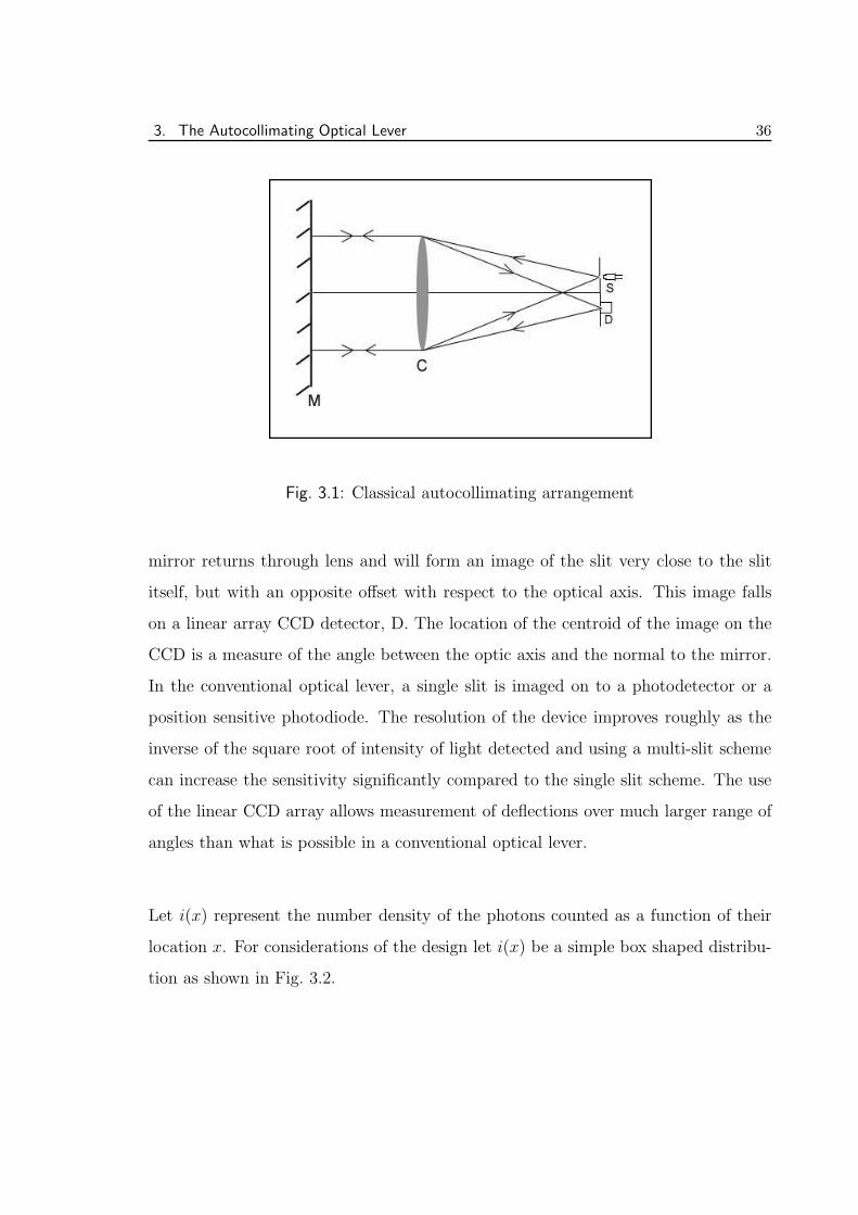
3. The Autocollimating Optical Lever 36
Fig. 3.1: Classical autocollimating arrangement
mirror returns through lens and will form an image of the slit very close to the slit
itself, but with an opposite offset with respect to the optical axis. This image falls
on a linear array CCD detector, D. The location of the centroid of the image on the
CCD is a measure of the angle between the optic axis and the normal to the mirror.
In the conventional optical lever, a single slit is imaged on to a photodetector or a
position sensitive photodiode. The resolution of the device improves roughly as the
inverse of the square root of intensity of light detected and using a multi-slit scheme
can increase the sensitivity significantly compared to the single slit scheme. The use
of the linear CCD array allows measurement of deflections over much larger range of
angles than what is possible in a conventional optical lever.
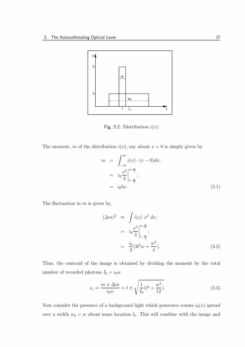
Let i(x) represent the number density of the photons counted as a function of their
location x. For considerations of the design let i(x) be a simple box shaped distribu-
tion as shown in Fig. 3.2.
3. The Autocollimating Optical Lever 37
Fig. 3.2: Distribution i(x)
The moment, m of the distribution i(x), say about x = 0 is simply given by
m =
∫ ∞
−∞i(x) · (x− 0)dx;
= i0x2
2
∣
∣
∣
∣
l+w2
l−w2
;
= i0lw. (3.1)
The fluctuation in m is given by,
(∆m)2 ≈∫
i(x) x2 dx;
= i0x3
3
∣
∣
∣
∣
l+w2
l−w2
;
=i03(3l2w +
w3
4). (3.2)
Thus, the centroid of the image is obtained by dividing the moment by the total
number of recorded photons I0 = i0w
xc =m±∆m
i0w= l ±
√
1
I0(l2 +
w2
12). (3.3)
Now consider the presence of a background light which generates counts ib(x) spread
over a width wb > w about some location lb. This will combine with the image and
3. The Autocollimating Optical Lever 38
generate a new centroid given by
xb =I0l + IblbI0 + Ib
±√
I0
(I0 + Ib)2 (l
2 +w2
12) +
Ib
(I0 + Ib)2 (l
2b +
wb2
12).
(3.4)
The presence of such a background induces both a systematic uncertainty and an
additional statistical uncertainty which can be large.
One element in the design of our optical lever is a strategy to eliminate the error
due to background light. From the total intensity field it = i(x) + ib(x) we subtract
ib + 3√ibpp
where p is the width of the digitizing pixel which is much smaller than w
and wb. δ = 3√ibpp
is the statistical fluctuation in the background light. After such a
subtraction we generate a new intensity field given by
in = {i(x) + ib(x)} − ib + 3
√
ibp
(3.5)
≈ i(x)− 3δ for in > 0.
= 0 for in < 0. (3.6)
The new centroid calculated with this in is given by
xn = l ±
√
(l2 + w2
12)
I0 − 3δw. (3.7)
Notice that xn ≈ xc when the fluctuation in the background intensity, δ, are small.
The second element in the design involves having multiple slits and corresponding
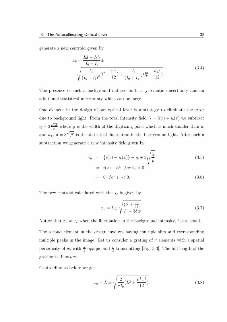
multiple peaks in the image. Let us consider a grating of ν elements with a spatial
periodicity of w, with w2opaque and w
2transmitting [Fig. 3.3]. The full length of the
grating is W = νw.
Centroiding as before we get
xg = L±√
2
νI0(L2 +
ν2w2
12). (3.8)
3. The Autocollimating Optical Lever 39
Fig. 3.3: Grating
The uncertainty in xg is much larger than that in xc and is about√2ν∆xc. This larger
uncertainty is essentially due to the fact that the width of the light distribution has
increased ν-fold.
To overcome this, consider a set of ν fiducial points xi, i = 1, 2, ..., ν, spaced at
intervals of w. The centroid of the image of the individual grating elements with
respect to the corresponding fiducial elements is given by
xci = x0ci ±
√
1
2I0(w2
4+
w2
12). (3.9)
Averaging all the xci
x =
∑
x0ci
ν±√
w2
6νI0. (3.10)
The precision in the determination of the centroid is substantially improved in this
case as opposed to Eqn. 3.8. It is as though the photon density of an individual
image of the slit has been increased by a factor ν. Since, the illumination of the slit is
limited by the brightness temperature of the source, the above method of decreasing
the statistical uncertainties proves useful.
The considerations related to the spacing of the grating are straightforward. The
3. The Autocollimating Optical Lever 40
mirror whose deflection angle is to be measured is smaller than the size of the auto-
collimator lens and as such determines the diffraction width of the image of the slit.
Thus, the width a0 of the opaque region between the slits may be taken as twice the
full width of the diffraction width due to the mirror:
a0 = 21.22λ
dmf. (3.11)
Here dm is the diameter of the mirror and f the focal length of the lens. The width
at of the transparent part of the grating should be chosen such that the width of
its image covers at least ∼ 5 pixels, so that the spatial digitization of the image is
adequate and does not lead to inadequate sampling of the possible asymmetries in
the image profile.
at +1.22λ
dmf & 5p. (3.12)
Although one would like to keep at as small as possible in an attempt to improve
the angular resolution of the optical lever, it is necessary to keep at to be at least as
large as the diffraction width itself to achieve a bright enough image, i.e., at ∼ 2.5p.
Further, it may be advantageous to choose its width large enough so that the light
illuminating it does not get diffracted away even beyond the periphery of the lens.
Thus, the grating constant a = a0 + at and it is of the order of four to five times the
diffraction width of the mirror.
3.2 Construction of the Optical Lever
A sketch of the optical lever is shown in Fig. 3.4. It consists of an array of slits made
with a photographic plate with transparent slits of 30 µm width, 90 in number, sepa-
rated from each other with dark regions of 120 µm width (opacity of the dark regions
is < 100%). This array is illuminated by light emanating from a brightly illuminated
ground glass sheet placed about five millimeters behind the array. A bank of red
LEDs which emit in a forward cone angle of ∼ 15 degree illuminate the ground glass
sheet with overlapping circles of light. This increases the brightness and uniformity of
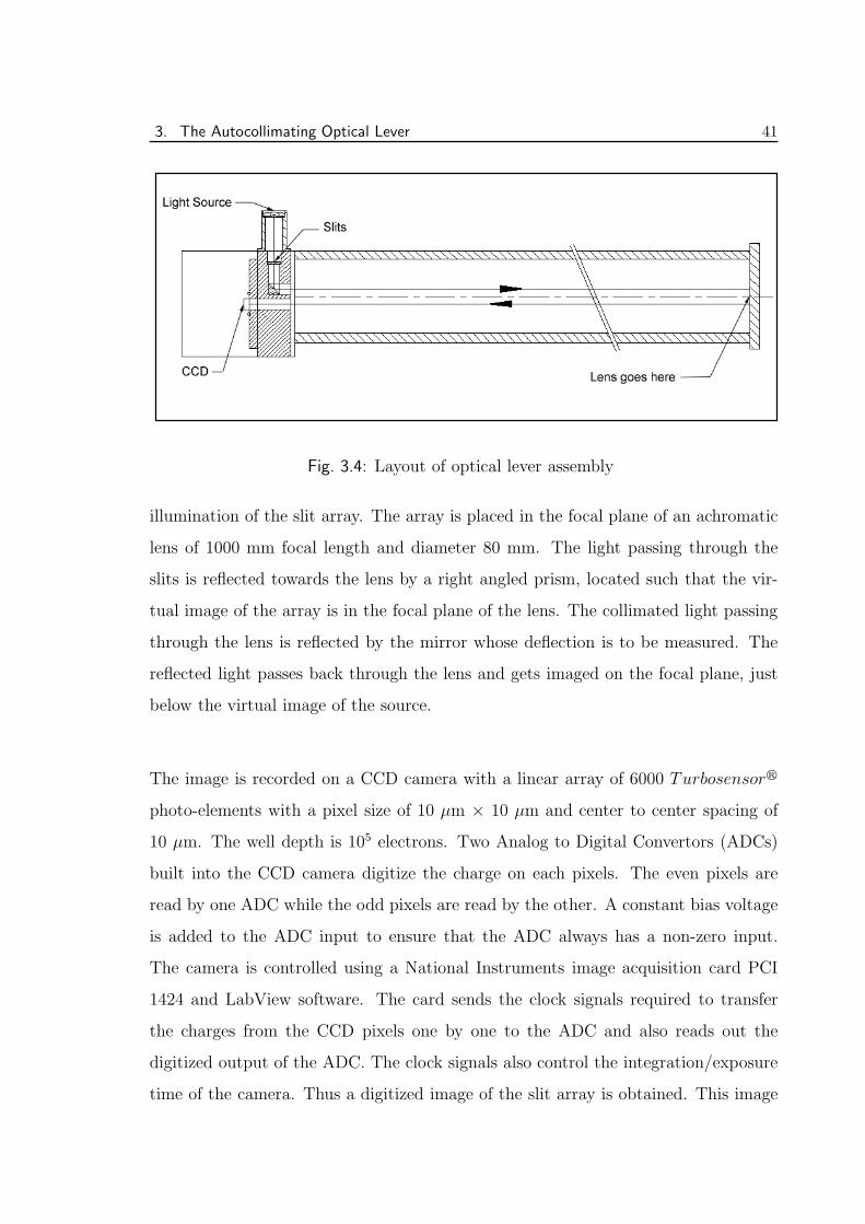
3. The Autocollimating Optical Lever 41
Fig. 3.4: Layout of optical lever assembly
illumination of the slit array. The array is placed in the focal plane of an achromatic
lens of 1000 mm focal length and diameter 80 mm. The light passing through the
slits is reflected towards the lens by a right angled prism, located such that the vir-
tual image of the array is in the focal plane of the lens. The collimated light passing
through the lens is reflected by the mirror whose deflection is to be measured. The
reflected light passes back through the lens and gets imaged on the focal plane, just
below the virtual image of the source.
The image is recorded on a CCD camera with a linear array of 6000 Turbosensorr
photo-elements with a pixel size of 10 µm × 10 µm and center to center spacing of
10 µm. The well depth is 105 electrons. Two Analog to Digital Convertors (ADCs)
built into the CCD camera digitize the charge on each pixels. The even pixels are
read by one ADC while the odd pixels are read by the other. A constant bias voltage
is added to the ADC input to ensure that the ADC always has a non-zero input.
The camera is controlled using a National Instruments image acquisition card PCI
1424 and LabView software. The card sends the clock signals required to transfer
the charges from the CCD pixels one by one to the ADC and also reads out the
digitized output of the ADC. The clock signals also control the integration/exposure
time of the camera. Thus a digitized image of the slit array is obtained. This image
3. The Autocollimating Optical Lever 42
3000 3010 3020 3030 3040 3050
0
50
100
150
200
CC
D C
ount
s
Pixel Number
Fig. 3.5: A sample image of the slits falling on the CCD
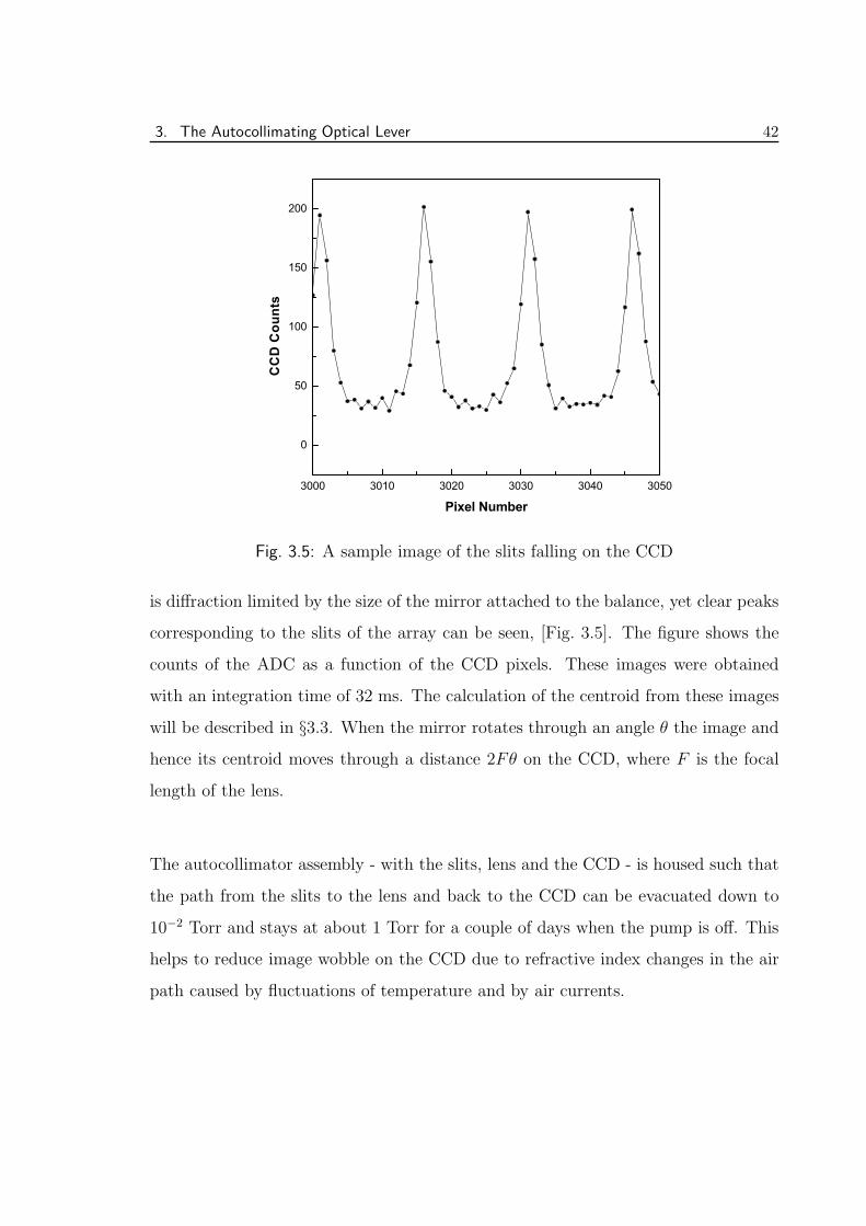
is diffraction limited by the size of the mirror attached to the balance, yet clear peaks
corresponding to the slits of the array can be seen, [Fig. 3.5]. The figure shows the
counts of the ADC as a function of the CCD pixels. These images were obtained
with an integration time of 32 ms. The calculation of the centroid from these images
will be described in §3.3. When the mirror rotates through an angle θ the image and
hence its centroid moves through a distance 2Fθ on the CCD, where F is the focal
length of the lens.
The autocollimator assembly - with the slits, lens and the CCD - is housed such that
the path from the slits to the lens and back to the CCD can be evacuated down to
10−2 Torr and stays at about 1 Torr for a couple of days when the pump is off. This
helps to reduce image wobble on the CCD due to refractive index changes in the air
path caused by fluctuations of temperature and by air currents.
3. The Autocollimating Optical Lever 43
3.3 Implementation of the Centroiding Algorithm
The centroid of the image is proportional to the angle the normal to the mirror
subtends with respect to the optic axis. The first step in the determination of the
centroid is to subtract from the individual pixel values ci the dark current and the
bias. The average value of the sum of dark and bias, di for each pixel is estimated
from 100 frames without any light falling on the CCD. Accordingly we set the effective
counts mi as,
mi = ci − di for di < ci
mi = 0 for di > ci (3.13)
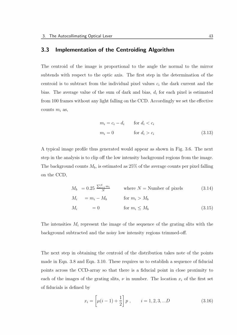
A typical image profile thus generated would appear as shown in Fig. 3.6. The next
step in the analysis is to clip off the low intensity background regions from the image.
The background counts Mb, is estimated as 25% of the average counts per pixel falling
on the CCD,
Mb = 0.25PN
i=1mi
Nwhere N = Number of pixels (3.14)
Mi = mi −Mb for mi > Mb
Mi = 0 for mi ≤ Mb (3.15)
The intensities Mi represent the image of the sequence of the grating slits with the
background subtracted and the noisy low intensity regions trimmed-off.
The next step in obtaining the centroid of the distribution takes note of the points
made in Eqn. 3.8 and Eqn. 3.10. These requires us to establish a sequence of fiducial
points across the CCD-array so that there is a fiducial point in close proximity to
each of the images of the grating slits, ν in number. The location xi of the first set
of fiducials is defined by
xi =
[
µ(i− 1) +1
2
]
p , i = 1, 2, 3, ...D (3.16)
3. The Autocollimating Optical Lever 44
where µ is the width of the each slit image in pixels (= 15 in our case) and D is the
total number of fiducial points.
Now computing the centroids of the intensity peaks that lie just ahead of each of
these fiducials and averaging we get the effective location of the image
x =L∑
k=1
′(
∑k+µ−1j=k Mj [{(j − 1) + 1
2}p− xk]
∑k+µ−1j=k Mj
)
(3.17)
Notice that in the averaging process we have to include only those values of k for
which all Msj (j = k to k + µ− 1) are not zero; this is indicated with a prime on the
outer summation sign. This procedure is similar to folding the image ν-times over
so that all the peaks line up on each other. x thus obtained is the centroid distance
modulo µp i.e., the mantissa. This may be added to a constant xc defined by
xc =
L∑
i=1
′ xi
ν(3.18)
to get the complete centroid X :
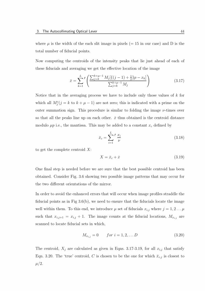
X = xc + x (3.19)
One final step is needed before we are sure that the best possible centroid has been
obtained. Consider Fig. 3.6 showing two possible image patterns that may occur for
the two different orientations of the mirror.
In order to avoid the enhanced errors that will occur when image profiles straddle the
fiducial points as in Fig 3.6(b), we need to ensure that the fiducials locate the image
well within them. To this end, we introduce µ set of fiducials xi,j where j = 1, 2 . . . µ
such that xi,j+1 = xi,j + 1. The image counts at the fiducial locations, Mxi,jare
scanned to locate fiducial sets in which,
Mxi,j= 0 for i = 1, 2, . . .D (3.20)
The centroid, Xj are calculated as given in Eqns. 3.17-3.19, for all xi,j that satisfy
Eqn. 3.20. The ‘true’ centroid, C is chosen to be the one for which xc,j is closest to
µ/2.
3. The Autocollimating Optical Lever 45
Fig. 3.6: Two possible image profiles with respect to the fiducial location, k; profile
in panel (a) will give an accurate centroid as per Eqn.3.19; profile in panel
(b) will have larger errors, since the centroid is calculated between k and
k + µ
3.4 Tests and characteristics of the optical lever
Several tests were performed to characterize the optical lever. The first was to study
the dark and bias counts of the CCD pixels. In the CCD the first and last 2 pixels
are internally shielded from light and are used by the CCD electronics to clamp the
dark and bias. The bias voltage applied to the ADC convertor, is adjusted such that
ADC output corresponding to the charges on these pixels is locked at 4-5 counts.
This keeps a check on drifts due to the internal electronics. Over and above this,
the counts in each pixel of the CCD were monitored for an exposure time of 32 ms
without any light falling on the CCD. 100 such points were averaged for each pixel to
determine the average sum of dark and bias of each pixel. This was later subtracted
from every frame acquired, to determine the dark and bias subtracted counts per pixel.
The diffraction limited image of the 30 µm slits falling on the CCD are 5 pixels wide
and are separated by 15 pixels. For an integration time of 32 ms, the peaks are at 200
counts compared to the saturation counts of 255 (with 8 bit digitization). The counts
in the region between the peaks is at 40 as against the dark counts of 5 in the regions
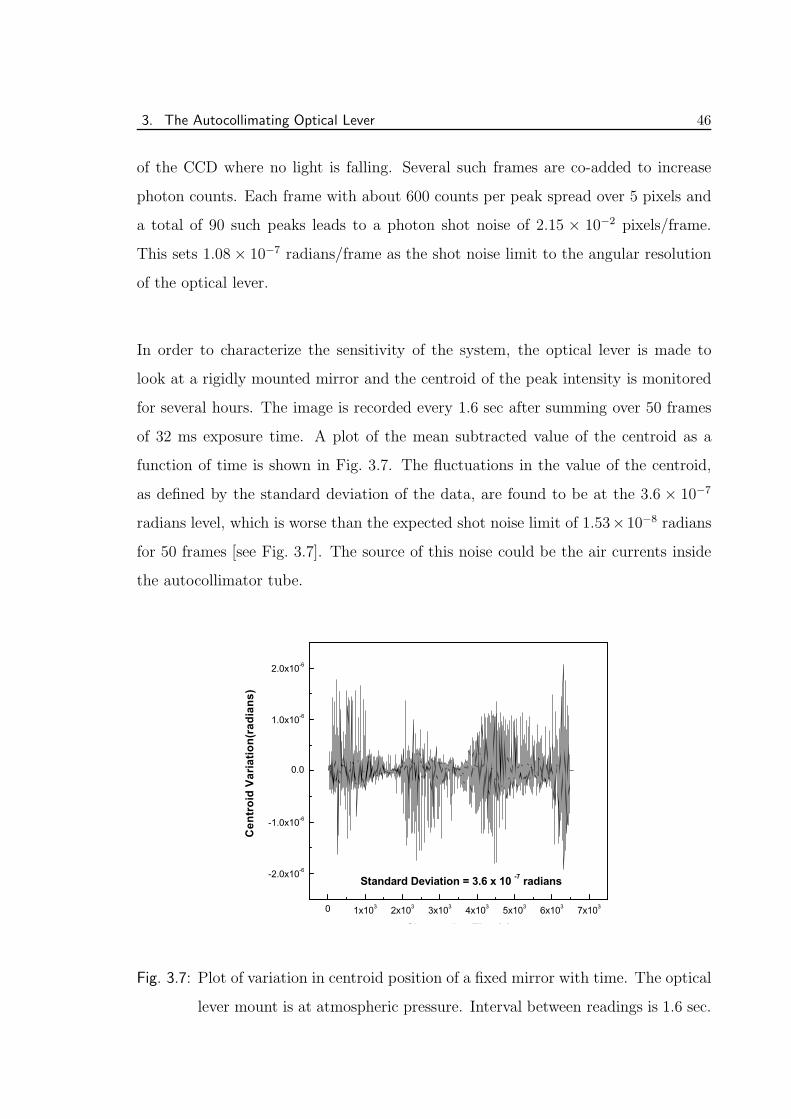
3. The Autocollimating Optical Lever 46
of the CCD where no light is falling. Several such frames are co-added to increase
photon counts. Each frame with about 600 counts per peak spread over 5 pixels and
a total of 90 such peaks leads to a photon shot noise of 2.15 × 10−2 pixels/frame.
This sets 1.08× 10⁻⁷ radians/frame as the shot noise limit to the angular resolution
of the optical lever.
In order to characterize the sensitivity of the system, the optical lever is made to
look at a rigidly mounted mirror and the centroid of the peak intensity is monitored
for several hours. The image is recorded every 1.6 sec after summing over 50 frames
of 32 ms exposure time. A plot of the mean subtracted value of the centroid as a
function of time is shown in Fig. 3.7. The fluctuations in the value of the centroid,
as defined by the standard deviation of the data, are found to be at the 3.6 × 10⁻⁷
radians level, which is worse than the expected shot noise limit of 1.53×10⁻⁸ radians
for 50 frames [see Fig. 3.7]. The source of this noise could be the air currents inside
the autocollimator tube.
0 1x10³ 2x10³ 3x10³ 4x10³ 5x10³ 6x10³ 7x10³
-2.0x10⁻⁶
-1.0x10⁻⁶
0.0
1.0x10⁻⁶
2.0x10⁻⁶
Cen
troi
d Va
riatio
n(ra
dian
s)
Observation Time(s)
Standard Deviation = 3.6 x 10 -7 radians
Fig. 3.7: Plot of variation in centroid position of a fixed mirror with time. The optical
lever mount is at atmospheric pressure. Interval between readings is 1.6 sec.
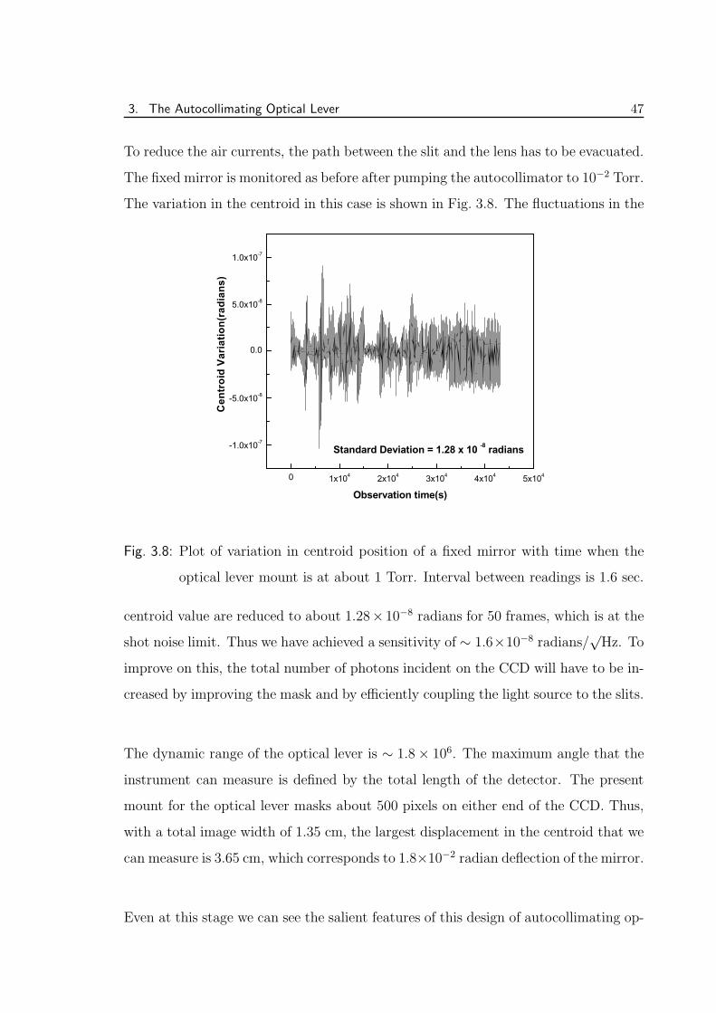
3. The Autocollimating Optical Lever 47
To reduce the air currents, the path between the slit and the lens has to be evacuated.
The fixed mirror is monitored as before after pumping the autocollimator to 10−2 Torr.
The variation in the centroid in this case is shown in Fig. 3.8. The fluctuations in the
0 1x10⁴ 2x10⁴ 3x10⁴ 4x10⁴ 5x10⁴
-1.0x10⁻⁷
-5.0x10⁻⁸
0.0
5.0x10⁻⁸
1.0x10⁻⁷
C
entr
oid
Varia
tion(
radi
ans)
Observation time(s)
Standard Deviation = 1.28 x 10 -8 radians
Fig. 3.8: Plot of variation in centroid position of a fixed mirror with time when the
optical lever mount is at about 1 Torr. Interval between readings is 1.6 sec.
centroid value are reduced to about 1.28×10⁻⁸ radians for 50 frames, which is at the
shot noise limit. Thus we have achieved a sensitivity of ∼ 1.6×10⁻⁸ radians/√Hz. To
improve on this, the total number of photons incident on the CCD will have to be in-
creased by improving the mask and by efficiently coupling the light source to the slits.
The dynamic range of the optical lever is ∼ 1.8× 10⁶. The maximum angle that the
instrument can measure is defined by the total length of the detector. The present
mount for the optical lever masks about 500 pixels on either end of the CCD. Thus,
with a total image width of 1.35 cm, the largest displacement in the centroid that we
can measure is 3.65 cm, which corresponds to 1.8×10⁻² radian deflection of the mirror.
Even at this stage we can see the salient features of this design of autocollimating op-
References 48
tical lever: it is capable of measuring angles with a sensitivity of ∼ 10−8 radians/√Hz
and has a dynamic range exceeding a few millions. These features are quite unique.
With a better mask and light source we hope to reach a sensitivity of 3 × 10⁻⁹
radian/√Hz without sacrificing the dynamic range.
References
[1] R. Cowsik et al. Torsion Balance Experiment for Measurement of Weak Forces in
Nature. Indian Journal of Pure & Applied Physics, 27:691–709, 1989.
[2] R. V. Jones. Some Points in the Design of Optical Levers and Amplifiers. Pro-
ceedings of the Physical Society B, 64:469–482, June 1951.
[3] R. V. Jones and J. C. S. Richards. CORRESPONDENCE: Recording optical
lever. Journal of Scientific Instruments, 36:199, April 1959.
4. CHARACTERIZATION OF THE
APPARATUS
Abstract: This chapter presents the tests and characterizations performed on the ex-
perimental apparatus.
4.1 The Torsional Pendulum
The force transducer in our experiment is a torsional pendulum. The sensitivity of
the torsional pendulum to any torque acting on it is related to the moment of inertia,
I of the mass element suspended and torsional constant of the suspension fibre, κ.
These parameters determine the time period of oscillation of the pendulum. The
period, Tb is given by
Tb = 2π
√
I
κ.
Another important parameter of an oscillator is its quality factor, Q. It is a measure
of the damping in the system and is defined as the ratio of time taken for the ampli-
tude of the oscillator to fall by 1/e to the time period of the oscillator.
In order to characterize our torsional pendulum, it was allowed to oscillate freely inside
the vacuum chamber at a pressure of 4.0×10⁻⁸ Torr with an amplitude of ∼ 3.0×10⁻³
radians. The oscillations are monitored continuously for about a day. Fig. 4.1 shows
a few cycles of the oscillations. The time period and Q are obtained from by Fourier
power spectrum of this time series data. The power spectrum calculated from the Fast
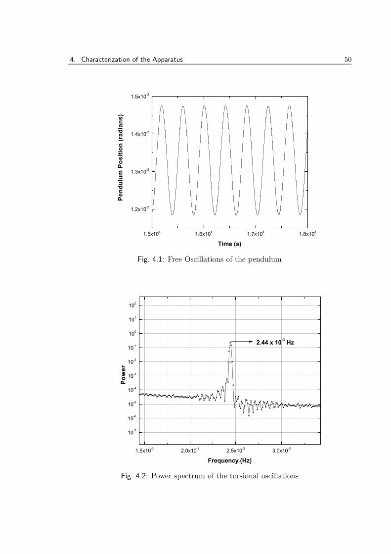
4. Characterization of the Apparatus 50
1.5x10⁴ 1.6x10⁴ 1.7x10⁴ 1.8x10⁴
1.2x10⁻²
1.3x10⁻²
1.4x10⁻²
1.5x10⁻²
Pend
ulum
Pos
ition
(rad
ians
)
Time (s)
Fig. 4.1: Free Oscillations of the pendulum
1.5x10⁻³ 2.0x10⁻³ 2.5x10⁻³ 3.0x10⁻³
10-7
10-6
10-5
10-4
10-3
10-2
10-1
100
101
102
Frequency (Hz)
Power
2.44 x 10⁻³ Hz
Fig. 4.2: Power spectrum of the torsional oscillations
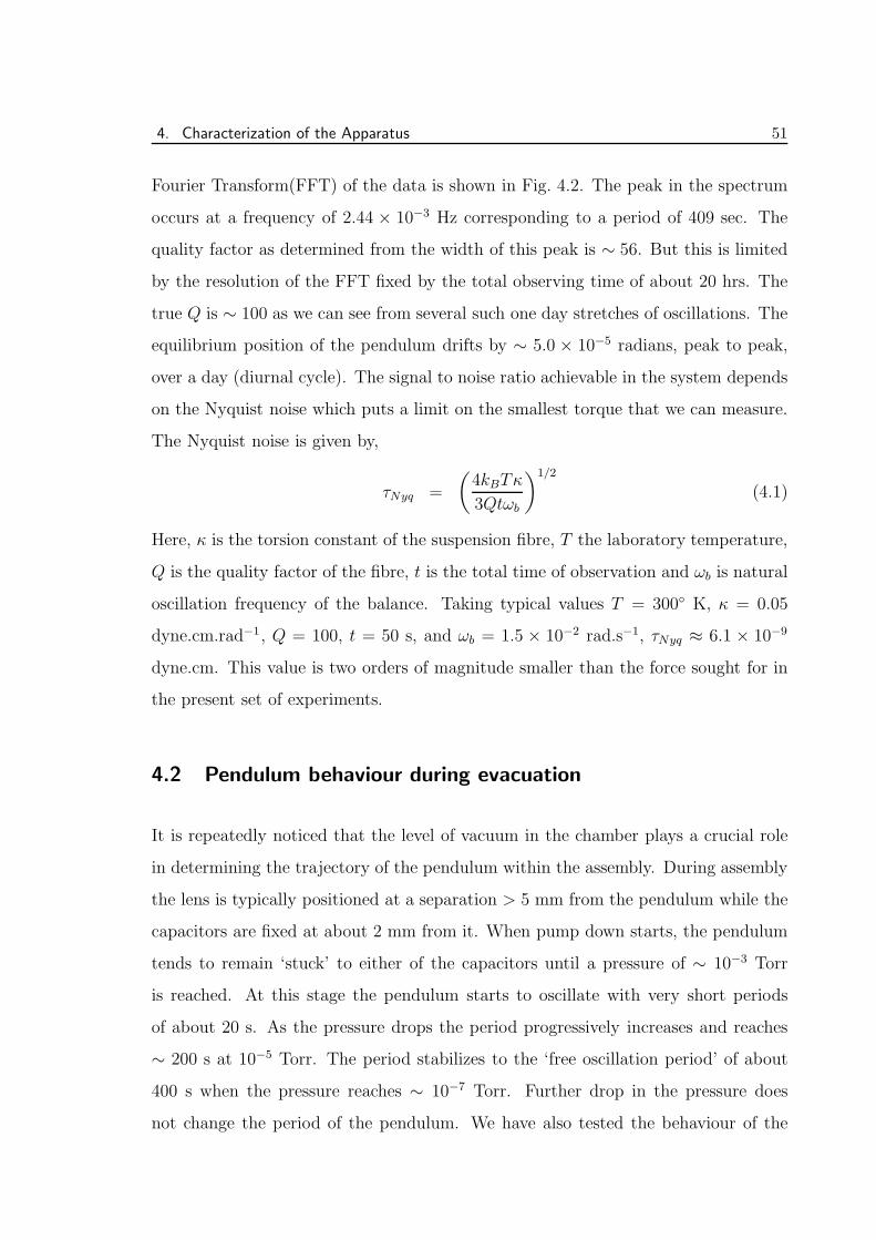
4. Characterization of the Apparatus 51
Fourier Transform(FFT) of the data is shown in Fig. 4.2. The peak in the spectrum
occurs at a frequency of 2.44 × 10⁻³ Hz corresponding to a period of 409 sec. The
quality factor as determined from the width of this peak is ∼ 56. But this is limited
by the resolution of the FFT fixed by the total observing time of about 20 hrs. The
true Q is ∼ 100 as we can see from several such one day stretches of oscillations. The
equilibrium position of the pendulum drifts by ∼ 5.0 × 10⁻⁵ radians, peak to peak,
over a day (diurnal cycle). The signal to noise ratio achievable in the system depends
on the Nyquist noise which puts a limit on the smallest torque that we can measure.
The Nyquist noise is given by,
τNyq =
(
4kBTκ
3Qtωb
)1/2
(4.1)
Here, κ is the torsion constant of the suspension fibre, T the laboratory temperature,
Q is the quality factor of the fibre, t is the total time of observation and ωb is natural
oscillation frequency of the balance. Taking typical values T = 300◦ K, κ = 0.05
dyne.cm.rad−1, Q = 100, t = 50 s, and ωb = 1.5 × 10⁻² rad.s−1, τNyq ≈ 6.1 × 10⁻⁹
dyne.cm. This value is two orders of magnitude smaller than the force sought for in
the present set of experiments.
4.2 Pendulum behaviour during evacuation
It is repeatedly noticed that the level of vacuum in the chamber plays a crucial role
in determining the trajectory of the pendulum within the assembly. During assembly
the lens is typically positioned at a separation > 5 mm from the pendulum while the
capacitors are fixed at about 2 mm from it. When pump down starts, the pendulum
tends to remain ‘stuck’ to either of the capacitors until a pressure of ∼ 10−3 Torr
is reached. At this stage the pendulum starts to oscillate with very short periods
of about 20 s. As the pressure drops the period progressively increases and reaches
∼ 200 s at 10−5 Torr. The period stabilizes to the ‘free oscillation period’ of about
400 s when the pressure reaches ∼ 10−7 Torr. Further drop in the pressure does
not change the period of the pendulum. We have also tested the behaviour of the
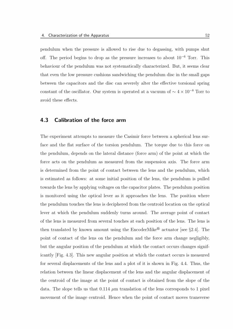
4. Characterization of the Apparatus 52
pendulum when the pressure is allowed to rise due to degassing, with pumps shut
off. The period begins to drop as the pressure increases to about 10−6 Torr. This
behaviour of the pendulum was not systematically characterized. But, it seems clear
that even the low pressure cushions sandwiching the pendulum disc in the small gaps
between the capacitors and the disc can severely alter the effective torsional spring
constant of the oscillator. Our system is operated at a vacuum of ∼ 4× 10⁻⁸ Torr to
avoid these effects.
4.3 Calibration of the force arm
The experiment attempts to measure the Casimir force between a spherical lens sur-
face and the flat surface of the torsion pendulum. The torque due to this force on
the pendulum, depends on the lateral distance (force arm) of the point at which the
force acts on the pendulum as measured from the suspension axis. The force arm
is determined from the point of contact between the lens and the pendulum, which
is estimated as follows: at some initial position of the lens, the pendulum is pulled
towards the lens by applying voltages on the capacitor plates. The pendulum position
is monitored using the optical lever as it approaches the lens. The position where
the pendulum touches the lens is deciphered from the centroid location on the optical
lever at which the pendulum suddenly turns around. The average point of contact
of the lens is measured from several touches at each position of the lens. The lens is
then translated by known amount using the EncoderMiker actuator [see §2.4]. The
point of contact of the lens on the pendulum and the force arm change negligibly,
but the angular position of the pendulum at which the contact occurs changes signif-
icantly [Fig. 4.3]. This new angular position at which the contact occurs is measured
for several displacements of the lens and a plot of it is shown in Fig. 4.4. Thus, the
relation between the linear displacement of the lens and the angular displacement of
the centroid of the image at the point of contact is obtained from the slope of the
data. The slope tells us that 0.114 µm translation of the lens corresponds to 1 pixel
movement of the image centroid. Hence when the point of contact moves transverse
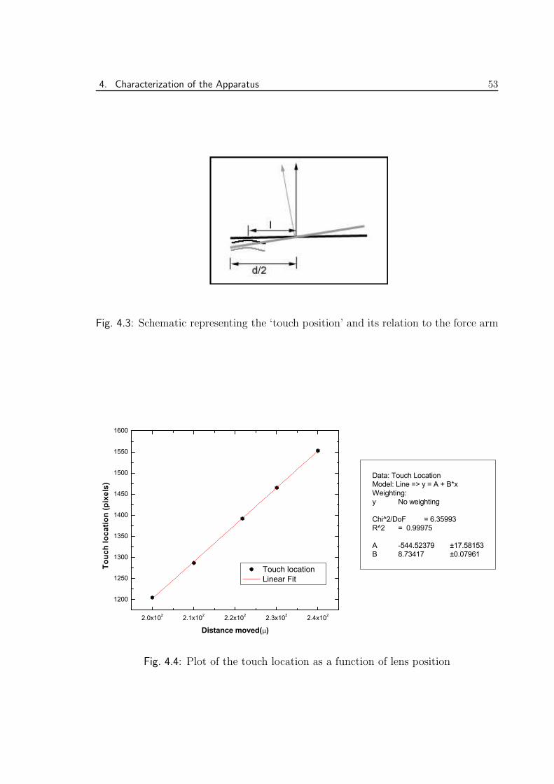
4. Characterization of the Apparatus 53
Fig. 4.3: Schematic representing the ‘touch position’ and its relation to the force arm
2.0x10² 2.1x10² 2.2x10² 2.3x10² 2.4x10²
1200
1250
1300
1350
1400
1450
1500
1550
1600
Data: Touch LocationModel: Line => y = A + B*xWeighting: y No weighting Chi^2/DoF = 6.35993R^2 = 0.99975 A -544.52379 ±17.58153B 8.73417 ±0.07961
Touc
h lo
catio
n (p
ixel
s)
Distance moved( )
Touch location Linear Fit
Fig. 4.4: Plot of the touch location as a function of lens position
4. Characterization of the Apparatus 54
to the plane of the pendulum (towards or away from the lens) by 0.114 µm, image
shifts by 1 pixel. From the optical lever parameters, we know that a image displace-
ment of 1 pixel corresponds to a transverse movement of 0.2 µm at the edge of the
pendulum disc which is at d/2 = 40 mm from the suspension axis [Fig. 4.3]. Thus
the force arm l or point of contact is at 22.8 mm from the axis of the pendulum.
5. CASIMIR FORCE MEASUREMENT -
STRATEGY, DATA ACQUISITION AND
ANALYSIS
Abstract: The basic procedures followed in our experiment will be described in this
chapter. The chapter begins with an overview of the forces influencing our torsion
pendulum transducer and goes on to describe how the data is acquired in order to
comprehend these. The analysis of this data to extract information about Casimir
force is then discussed in detail. There is clear evidence for the finite temperature
Casimir force, detected for the first time, in the analyzed data.
5.1 Strategy of the experiment
The main objective of the experiment is to measure the force of attraction between a
fixed lens and a flat plate suspended as a torsional pendulum. In the absence of the
lens, the only torque acting on the pendulum is the restoring torque from the fibre.
As the lens is brought close to the fibre, various forces begin to act on the pendulum.
The basic torques acting on the pendulum when the pendulum oscillates near the
lens are the fibre restoring torque and the torques due to electrostatic and Casimir
force.
The presence of all these forces will introduce changes on the torsional oscillations of
the pendulum. Since these forces in general arise from potentials that differ from the
5. Casimir Force Measurement - Strategy, Data Acquisition and Analysis 56
quadratic harmonic potential due to the torsion in the fibre, they make the motion
of the pendulum anharmonic. As described in the previous chapters, we record the
angular position, θ of the fibre as a function of time, t. Thus the strategy adopted is
to extract information about the forces from the t versus θ data.
The free oscillations of a pendulum will be simple harmonic. The existence of other
potentials, besides the harmonic potential due to the fibre, will contribute to the
acceleration θ, thereby changing the simple linear relationship of θ with the amplitude
of the oscillations. If f(θ) is the net force on the pendulum then,
The torque on the pendulum,
τ(θ) = f(θ)l and (5.1)
Iθ = τ(θ) (5.2)
where l is the lateral distance of the point at which the force acts on the pendulum
as measured from the suspension axis, θ is the angular acceleration of the pendulum.
Similarly the angular velocity θ is related to the potential U(θ),
1
2Iθ2 + U(θ) = E = const. (5.3)
where τ(θ) = −∂U(θ)
∂θ(5.4)
Thus, by measuring θ or θ the potential and the forces that affect the pendulum can
be characterized.
5.1.1 Summary of Forces acting on the Pendulum
Several forces between the lens and the pendulum begin to become sizeable as they
approach each other to within about 100 µm. We now discuss the forces that play a
major role in the motion of the pendulum.
5. Casimir Force Measurement - Strategy, Data Acquisition and Analysis 57
Fibre restoring torque:
The restoring torque due to the fibre makes the pendulum execute simple harmonic
motion about a mean position, hereafter referred to as the ‘null’ position θ0. As is well
known, this torque always acts towards θ0 and in proportion to the deflection of the
torsion balance from this position. In the following descriptions, the distances and
the angles are measured with respect to the position of the lens as origin [Fig. 5.1].
During the experiment, the presence of other forces will generate new torques which
will shift the balance to a new equilibrium position θe. By appropriate rotation of the
shaft from which the balance is suspended, the equilibrium position θe is made to lie
between the lens at θl = 0, and θ0. The restoring torque, τfib and the acceleration,
θfib on the pendulum due to this torque are given by:
τfib(θ) = κ(θ0 − θ) (5.5)
θfib =κ
I(θ0 − θ) (5.6)
θfib = 2.46× 10⁻⁴(θ0 − θ) (5.7)
where κ is the torsion constant of the fibre, I the moment of inertia of the pendulum
and θ0 is the equilibrium position of the pendulum. Similarly the potential, Ufib and
the angular velocity, θfib are given by,
Ufib =κ
2(θ0 − θ)2 + const. (5.8)
It is convenient to write in general,
θ2fib = −2U
I+ const. (5.9)
≡ −UN + const. (5.10)
With this we may think of θ2 as just the negative of the normalized potential UN .
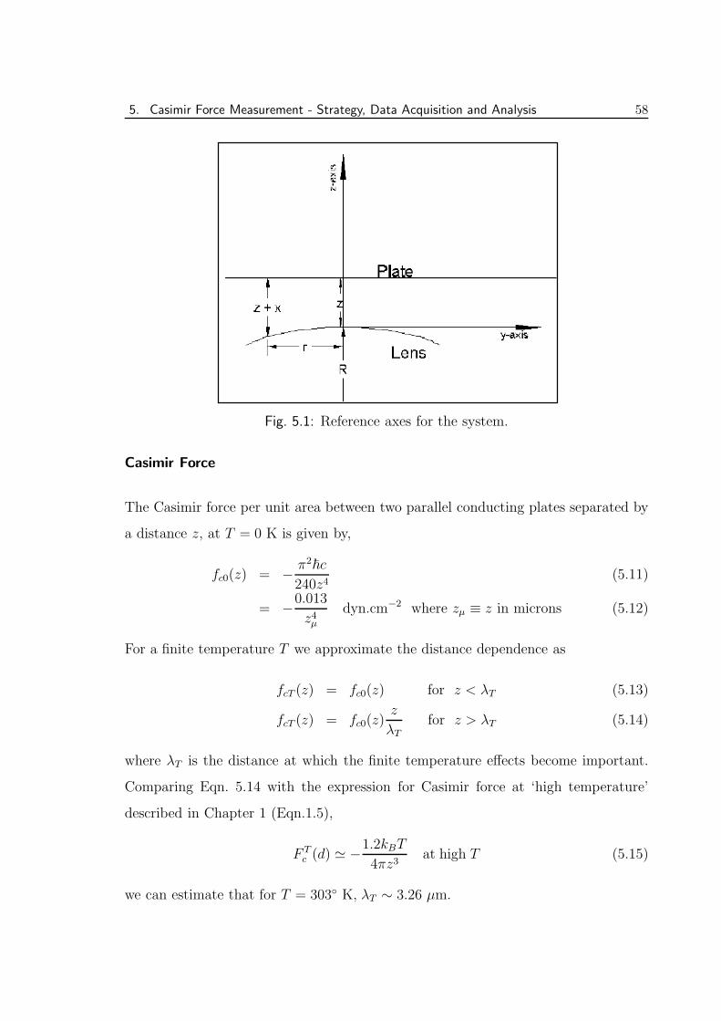
5. Casimir Force Measurement - Strategy, Data Acquisition and Analysis 58
Fig. 5.1: Reference axes for the system.
Casimir Force
The Casimir force per unit area between two parallel conducting plates separated by
a distance z, at T = 0 K is given by,
fc0(z) = − π2~c
240z4(5.11)
= −0.013
z4µdyn.cm−2 where zµ ≡ z in microns (5.12)
For a finite temperature T we approximate the distance dependence as
fcT (z) = fc0(z) for z < λT (5.13)
fcT (z) = fc0(z)z
λTfor z > λT (5.14)
where λT is the distance at which the finite temperature effects become important.
Comparing Eqn. 5.14 with the expression for Casimir force at ‘high temperature’
described in Chapter 1 (Eqn.1.5),
F Tc (d) ≃ −1.2kBT
4πz3at high T (5.15)
we can estimate that for T = 303◦ K, λT ∼ 3.26 µm.
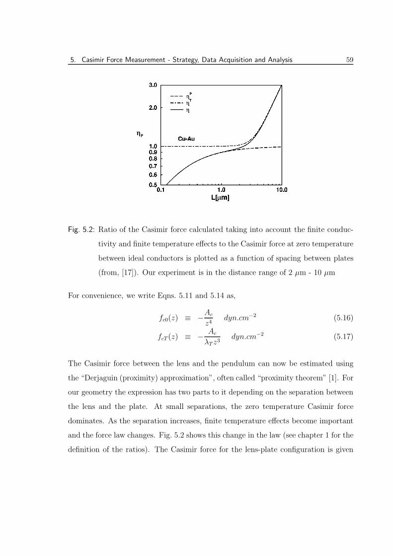
5. Casimir Force Measurement - Strategy, Data Acquisition and Analysis 59
Fig. 5.2: Ratio of the Casimir force calculated taking into account the finite conduc-
tivity and finite temperature effects to the Casimir force at zero temperature
between ideal conductors is plotted as a function of spacing between plates
(from, [17]). Our experiment is in the distance range of 2 µm - 10 µm
For convenience, we write Eqns. 5.11 and 5.14 as,
fc0(z) ≡ −Ac
z4dyn.cm−2 (5.16)
fcT (z) ≡ − Ac
λT z3dyn.cm−2 (5.17)
The Casimir force between the lens and the pendulum can now be estimated using
the “Derjaguin (proximity) approximation”, often called “proximity theorem” [1]. For
our geometry the expression has two parts to it depending on the separation between
the lens and the plate. At small separations, the zero temperature Casimir force
dominates. As the separation increases, finite temperature effects become important
and the force law changes. Fig. 5.2 shows this change in the law (see chapter 1 for the
definition of the ratios). The Casimir force for the lens-plate configuration is given
5. Casimir Force Measurement - Strategy, Data Acquisition and Analysis 60
by (see Appendix B for details),
fcl(z) = −2πRAc
3
[
1
z3− 1
(z + λT )3 +
3
2λT
{
1
(z + λT )2− 1
(z + xmax)2
}]
,(5.18)
for z < λT
fcl(z) = −πRAc
λT
{
1
z2− 1
(z + xmax)2
}
, for z > λT
where xmax = r2max
2Rand z = lθ is the separation between the lens and the plate,
R is the radius of curvature of the lens and rmax is the aperture radius of the lens
(Fig. 5.1). The potentials for the same configuration are,
Ucl(z) =πRAc
4
[
1
z2− 1
(z + λT )2 +
8
3λT
{
1
(z + λT )− 1
(z + xmax)
}]
, (5.19)
for z < λT
Ucl(z) =2πRAc
3λT
{
1
z− 1
(z + xmax)
}
for z > λT (5.20)
The angular velocity and acceleration due to Casimir force can be calculated using
Eqns. 5.3 and 5.4.
It may be noted that the roughness of the surface is not a major correction term to the
Casimir force in our experiment, since it focuses on Casimir force at relatively large
separations between the metal surfaces. However, the finite conductivity correction,
a reduction in force amounting to approximately 10% needs to be applied throughout
the measurement range.
Electrostatic Forces
There are various sources of electrostatic force between the lens and the plate. Several
effects lead to potential differences between metal coated surfaces even when they are
externally connected to ground [12, 13, 1]. Small difference in the contact potentials
in these connections can lead to potential differences between these surfaces. With
care, such potentials can be minimized to a few mV level. Another source of electro-
static interaction between the bodies are patch fields. These are microscopic electric
5. Casimir Force Measurement - Strategy, Data Acquisition and Analysis 61
potentials found on surfaces of metals. The different crystalline planes of a given ma-
terial can have work functions that can differ by as much as 1 V . If the coated metal
surface is a mosaic of random microscopic crystal planes, local potential differences
will occur between each of these micro-size patches. Surface contamination in the
metal coatings can also lead to local variations in the work function and also provide
sites for trapping electrical charges.
Force due to Capacitative coupling:
The conductive surfaces of the lens and the plate, form a capacitance which is given
by “proximity theorem” to be,
Cl = ǫ0〈A
d〉 (5.21)
= ǫ0
∫ r=rmax
r=0
2πrdr
[z + r2
2R]
(5.22)
= 2πRǫ0 ln
{
z + r2max
2R
z
}
(5.23)
where ǫ0 is the dielectric constant in free space, R is the radius of curvature of the
lens, z the separation between the lens and the pendulum in metres and rmax is the
aperture radius of the lens. If the voltage difference, V between the lens and the plate
were zero, the net force due to this capacitance will be zero. But potentials can be
present due to any of the reason mentioned above. The electrostatic potential energy
due to these between the lens and the plate is given by,
Uel =1
2ClV
2 (5.24)
= πRǫ0V2 ln
{
z + r2max
2R
z
}
(5.25)
The resulting capacitative force is given by,
fel = − d
dz[Uel] , (5.26)
≈ −πRǫ0V2
zfor r2max ≫ 2Rz. (5.27)
(5.28)
5. Casimir Force Measurement - Strategy, Data Acquisition and Analysis 62
We approximate the corrections to the above formula, due to surface roughness and
a variety of other causes and write for the torque,
τel = −πRǫ0V2
(θ − θr)(5.29)
(5.30)
where the roughness parameter θr will be determined self-consistently from the data.
The voltage V comprises of the applied voltage Vap, the D.C voltage V(0,dc) due to
contact potentials and other causes and V(0,ac) due to the stray pick up fields and
leakage, etc. This contributes to the normalized force a term,
θel = − πRǫ0V2
I(θ − θr). (5.31)
Force due to charges on the lens/pendulum:
Stray electric charges on the surfaces of the lens and the plate also lead to electrostatic
forces. The potential between these charges depends in detail on their distribution
on the surfaces and cannot be modeled easily [see for example, [10]]. An upper
limit to the strength of this force may be obtained by assuming that all the charge
is concentrated at the point of contact between the lens and the plate and that a
simple inverse square law applies for the force with an equidistance image charge.
The potential due this is given by,
Uqq =q2
4πǫ0zm, (5.32)
zm = 2z, the separation between the lens and the pendulum. (5.33)
The force and the acceleration on the pendulum due to it are,
fqq = − q2
4πǫ0z2m. (5.34)
Torque, τqq = − q2
16πǫ0lθ2, (5.35)
θqq = − q2
16πǫ0lIθ2, (5.36)
= −2.94× 10¹⁵q2
θ2. (5.37)
5. Casimir Force Measurement - Strategy, Data Acquisition and Analysis 63
where q is effective charge on the lens/pendulum. For a distributed charge the ∼ 1/θ2
dependence will change over to a slower dependence of ∼ 1/θ. This will be the case
with metallic surfaces when there are some residual charges on them.
Force due to charge and voltage on the lens:
One more source of electrostatic force is the combined effect of the charges and voltage
differences present. The electric field, E , due to these voltages, V interacts with the
charge, q to apply an additional force on the pendulum of the form,
fvq = −qE = −qV
z, (5.38)
Torque, τvq = −qV l
z, (5.39)
Acceleration, θ = −qV
Iθ, (5.40)
= −5.2× 10⁴qV
θ. (5.41)
V0 = V(0,dc)+V(0,ac); however, since the acceleration is linear in V as shown in Eqn 5.41
and the pick up voltages are at frequencies much higher than the frequency of oscilla-
tion of the balance at a few milliHertz, the A.C torques will average to zero and will
not contribute.
Gravitational force:
The gravitational attraction of the lens on the pendulum gives rise to a torque of
∼ 4 × 10⁻⁵ dyne.cm on it. This corresponds to the attraction between disc shaped
masses of approximately 10 g each separated by an effective distance of about 5 mm.
The ‘compensating plate’ (refer §2.5) is used to balance this gravitational torque
of the lens. The mass of the compensating plate is equal to that of the lens but
its position with respect to the torsion pendulum disc is not exactly the same as
the lens. Therefore, the cancellation of the gravitational torque is only approximate
and the residual gravitational torque on the pendulum is estimated to be ∼ 10−6
dyne.cm. This changes only by ∼ 10−8 dyne.cm when the lens is moved over the
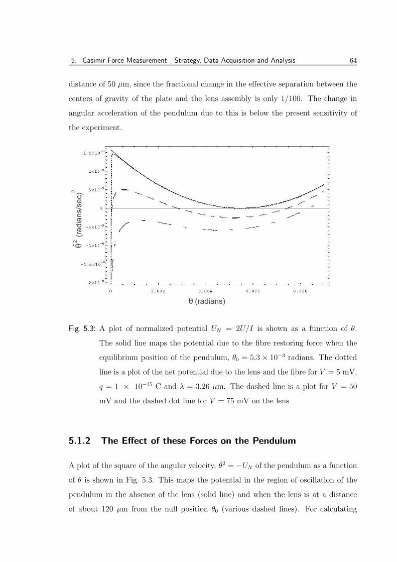
5. Casimir Force Measurement - Strategy, Data Acquisition and Analysis 64
distance of 50 µm, since the fractional change in the effective separation between the
centers of gravity of the plate and the lens assembly is only 1/100. The change in
angular acceleration of the pendulum due to this is below the present sensitivity of
the experiment.
Fig. 5.3: A plot of normalized potential UN = 2U/I is shown as a function of θ.
The solid line maps the potential due to the fibre restoring force when the
equilibrium position of the pendulum, θ0 = 5.3 × 10⁻³ radians. The dotted
line is a plot of the net potential due to the lens and the fibre for V = 5 mV,
q = 1 × 10⁻¹⁵ C and λ = 3.26 µm. The dashed line is a plot for V = 50
mV and the dashed dot line for V = 75 mV on the lens
5.1.2 The Effect of these Forces on the Pendulum
A plot of the square of the angular velocity, θ2 = −UN of the pendulum as a function
of θ is shown in Fig. 5.3. This maps the potential in the region of oscillation of the
pendulum in the absence of the lens (solid line) and when the lens is at a distance
of about 120 µm from the null position θ0 (various dashed lines). For calculating
5. Casimir Force Measurement - Strategy, Data Acquisition and Analysis 65
the potential due to the lens, the net voltage difference between the lens and the
pendulum V is set to 5 mV (dotted line), 50 mV (dashed line) and 75 mV (dashed
dot line). The net charge, q is taken to be 1× 10⁻¹⁵ C and the distance at which the
Casimir force changes from zero to finite temperature form, λ is taken to be 3.26 µm.
From the plot it can be seen that the presence of the electrostatic and Casimir forces,
considerably changes the potential between the lens and the plate. The potential is
highly attractive towards the lens for small angular separations. The angular distance
at which this change over to attractive potential happens depends on the net voltage
on the lens. Thus, when the voltage on the lens is 5 mV, the change over happens
at a distances of about 5 × 10⁻⁵ radians. As the voltage on the lens increases, the
change over point extends away from the lens. The equilibrium position of oscillation
of the pendulum is also shifted for voltages higher than 20 mV. The potential beyond
7 × 10⁻³ radians is shifted for higher voltages but is parallel to the pontetial due to
free fibre. The potential below 7 × 10⁻³ radians is flatter than the potential due to
free fibre. Thus the oscillation period of the pendulum is modified even for small
amplitude oscillations of the pendulum.
As the lens is brought close to the pendulum the signatures of the electrostatic forces
can be seen by looking at changes in:
(a) the equilibrium position of the pendulum,
(b) the time period of the pendulum, and
(c) the angular acceleration θ of the pendulum as a function of its angular position θ.
Since the Casimir force falls off more rapidly than the electrostatic force, to study
the effects of Casimir force, we need to go closer to the lens, i.e., < 1× 10⁻³ radians.
At those angular distances, the pendulum will no longer oscillate but will start to fall
5. Casimir Force Measurement - Strategy, Data Acquisition and Analysis 66
towards the lens. The force in that region then can be elucidated only from the θ
versus θ of the pendulum. Hence, to estimate Casimir force, we need to look at the θ
versus θ of the pendulum at angular distances of < 1× 10⁻³ radians.
To completely fathom the electrostatic forces though, in addition to measurements of
the changes on the pendulum as a function of lens position, knowledge about these
changes as a function of voltage on the lens are also essential. The force due to the
capacitive coupling increases as the square of the net voltage on the lens, while the
charge effect is linear in voltage. Hence, by studying the force dependance on the
voltage, an estimate of the effect of both the residual voltage and the charge on the
pendulum can be obtained.
5.2 Data Acquisition:
Despite considerable care taken during the assembly to minimize the voltages and
charges on the lens and the pendulum, certain residuals are unavoidably present in
the apparatus and it is essential to characterize these electrostatic forces. All the
earlier experiments that looked for Casimir forces have seen the effect of these forces
[8, 7, 16, 18, 24, 14, 4, 2]. Since the distance range in our experiment is larger than
the earlier experiments on Casimir force, electrostatic forces are a strong background.
Hence, the data acquisition was tuned to be able to estimate the electrostatic forces
and subtract them in order to look at the Casimir force at separations between 2 µm
- 10 µm.
The Casimir force falls off more rapidly with distance than the electrostatic forces.
Thus, at distances > 25 µm the electrostatics forces will dominate by more than two
orders of magnitude. At these separations corresponding to a angular distance of
> 1 × 10⁻³ radians, even for a net voltage, V of 75 mV between the lens and the
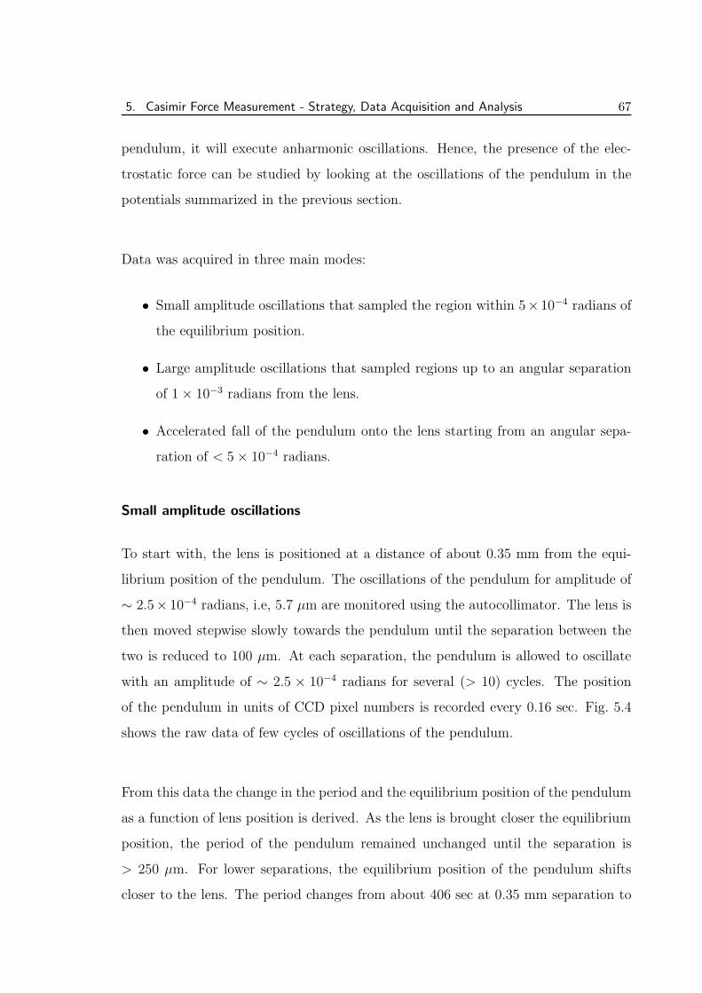
5. Casimir Force Measurement - Strategy, Data Acquisition and Analysis 67
pendulum, it will execute anharmonic oscillations. Hence, the presence of the elec-
trostatic force can be studied by looking at the oscillations of the pendulum in the
potentials summarized in the previous section.
Data was acquired in three main modes:
• Small amplitude oscillations that sampled the region within 5×10⁻⁴ radians of
the equilibrium position.
• Large amplitude oscillations that sampled regions up to an angular separation
of 1× 10⁻³ radians from the lens.
• Accelerated fall of the pendulum onto the lens starting from an angular sepa-
ration of < 5× 10⁻⁴ radians.
Small amplitude oscillations
To start with, the lens is positioned at a distance of about 0.35 mm from the equi-
librium position of the pendulum. The oscillations of the pendulum for amplitude of
∼ 2.5× 10⁻⁴ radians, i.e, 5.7 µm are monitored using the autocollimator. The lens is
then moved stepwise slowly towards the pendulum until the separation between the
two is reduced to 100 µm. At each separation, the pendulum is allowed to oscillate
with an amplitude of ∼ 2.5 × 10⁻⁴ radians for several (> 10) cycles. The position
of the pendulum in units of CCD pixel numbers is recorded every 0.16 sec. Fig. 5.4
shows the raw data of few cycles of oscillations of the pendulum.
From this data the change in the period and the equilibrium position of the pendulum
as a function of lens position is derived. As the lens is brought closer the equilibrium
position, the period of the pendulum remained unchanged until the separation is
> 250 µm. For lower separations, the equilibrium position of the pendulum shifts
closer to the lens. The period changes from about 406 sec at 0.35 mm separation to
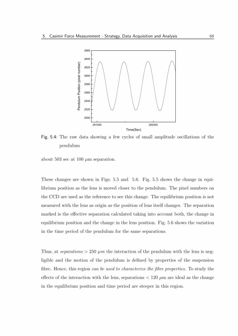
5. Casimir Force Measurement - Strategy, Data Acquisition and Analysis 68
281000 282000
2500
2520
2540
2560
2580
2600
2620
2640
2660
Pend
ulum
Pos
ition
(pix
el n
umbe
r)
Time(Sec)
Fig. 5.4: The raw data showing a few cycles of small amplitude oscillations of the
pendulum
about 503 sec at 100 µm separation.
These changes are shown in Figs. 5.5 and 5.6. Fig. 5.5 shows the change in equi-
librium position as the lens is moved closer to the pendulum. The pixel numbers on
the CCD are used as the reference to see this change. The equilibrium position is not
measured with the lens as origin as the position of lens itself changes. The separation
marked is the effective separation calculated taking into account both, the change in
equilibrium position and the change in the lens position. Fig. 5.6 shows the variation
in the time period of the pendulum for the same separations.
Thus, at separations > 250 µm the interaction of the pendulum with the lens is neg-
ligible and the motion of the pendulum is defined by properties of the suspension
fibre. Hence, this region can be used to characterize the fibre properties. To study the
effects of the interaction with the lens, separations < 120 µm are ideal as the change
in the equilibrium position and time period are steeper in this region.
5. Casimir Force Measurement - Strategy, Data Acquisition and Analysis 69
100 150 200 250 300 350 400
2420
2440
2460
2480
2500
2520
2540
2560
2580
Equi
libriu
m p
ositi
on (p
ixel
num
ber)
Separation( )
Fig. 5.5: The change in the equilibrium position of the pendulum as the lens is moved
closer to it.
100 150 200 250 300 350 400
400
420
440
460
480
500
520
Perio
d of
the
pend
ulum
(sec
)
Separation ( )
Fig. 5.6: The change in the time period of the pendulum as the lens is moved closer
to it.
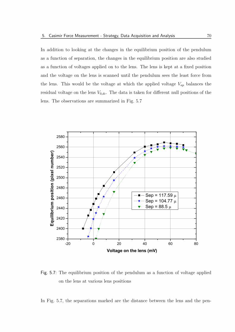
5. Casimir Force Measurement - Strategy, Data Acquisition and Analysis 70
In addition to looking at the changes in the equilibrium position of the pendulum
as a function of separation, the changes in the equilibrium position are also studied
as a function of voltages applied on to the lens. The lens is kept at a fixed position
and the voltage on the lens is scanned until the pendulum sees the least force from
the lens. This would be the voltage at which the applied voltage Vap balances the
residual voltage on the lens V0,dc. The data is taken for different null positions of the
lens. The observations are summarized in Fig. 5.7
-20 0 20 40 60 802380
2400
2420
2440
2460
2480
2500
2520
2540
2560
2580
Equi
libriu
m p
ositi
on (p
ixel
num
ber)
Voltage on the lens (mV)
Sep = 117.59 Sep = 104.77 Sep = 88.5
Fig. 5.7: The equilibrium position of the pendulum as a function of voltage applied
on the lens at various lens positions
In Fig. 5.7, the separations marked are the distance between the lens and the pen-
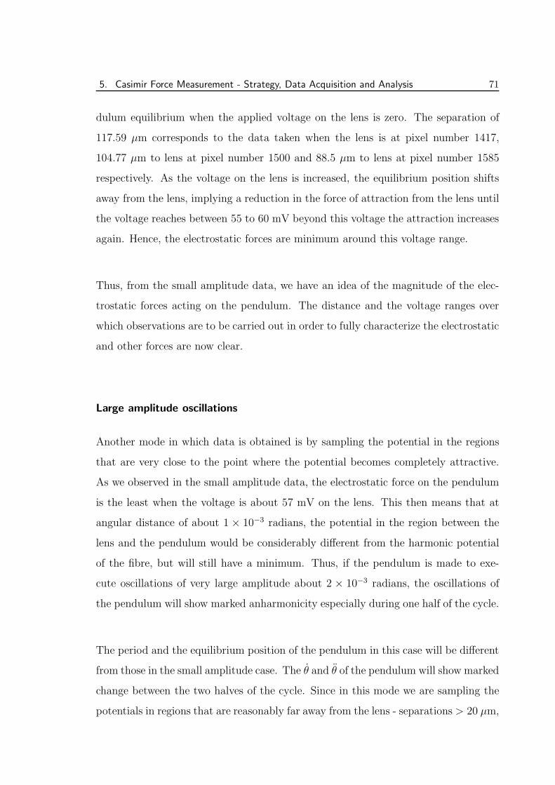
5. Casimir Force Measurement - Strategy, Data Acquisition and Analysis 71
dulum equilibrium when the applied voltage on the lens is zero. The separation of
117.59 µm corresponds to the data taken when the lens is at pixel number 1417,
104.77 µm to lens at pixel number 1500 and 88.5 µm to lens at pixel number 1585
respectively. As the voltage on the lens is increased, the equilibrium position shifts
away from the lens, implying a reduction in the force of attraction from the lens until
the voltage reaches between 55 to 60 mV beyond this voltage the attraction increases
again. Hence, the electrostatic forces are minimum around this voltage range.
Thus, from the small amplitude data, we have an idea of the magnitude of the elec-
trostatic forces acting on the pendulum. The distance and the voltage ranges over
which observations are to be carried out in order to fully characterize the electrostatic
and other forces are now clear.
Large amplitude oscillations
Another mode in which data is obtained is by sampling the potential in the regions
that are very close to the point where the potential becomes completely attractive.
As we observed in the small amplitude data, the electrostatic force on the pendulum
is the least when the voltage is about 57 mV on the lens. This then means that at
angular distance of about 1 × 10⁻³ radians, the potential in the region between the
lens and the pendulum would be considerably different from the harmonic potential
of the fibre, but will still have a minimum. Thus, if the pendulum is made to exe-
cute oscillations of very large amplitude about 2 × 10⁻³ radians, the oscillations of
the pendulum will show marked anharmonicity especially during one half of the cycle.
The period and the equilibrium position of the pendulum in this case will be different
from those in the small amplitude case. The θ and θ of the pendulum will show marked
change between the two halves of the cycle. Since in this mode we are sampling the
potentials in regions that are reasonably far away from the lens - separations > 20 µm,
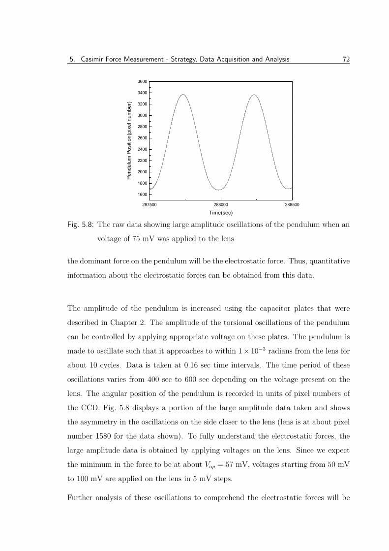
5. Casimir Force Measurement - Strategy, Data Acquisition and Analysis 72
287500 288000 288500
1600
1800
2000
2200
2400
2600
2800
3000
3200
3400
3600
Pend
ulum
Pos
ition
(pix
el n
umbe
r)
Time(sec)
Fig. 5.8: The raw data showing large amplitude oscillations of the pendulum when an
voltage of 75 mV was applied to the lens
the dominant force on the pendulum will be the electrostatic force. Thus, quantitative
information about the electrostatic forces can be obtained from this data.
The amplitude of the pendulum is increased using the capacitor plates that were
described in Chapter 2. The amplitude of the torsional oscillations of the pendulum
can be controlled by applying appropriate voltage on these plates. The pendulum is
made to oscillate such that it approaches to within 1× 10⁻³ radians from the lens for
about 10 cycles. Data is taken at 0.16 sec time intervals. The time period of these
oscillations varies from 400 sec to 600 sec depending on the voltage present on the
lens. The angular position of the pendulum is recorded in units of pixel numbers of
the CCD. Fig. 5.8 displays a portion of the large amplitude data taken and shows
the asymmetry in the oscillations on the side closer to the lens (lens is at about pixel
number 1580 for the data shown). To fully understand the electrostatic forces, the
large amplitude data is obtained by applying voltages on the lens. Since we expect
the minimum in the force to be at about Vap = 57 mV, voltages starting from 50 mV
to 100 mV are applied on the lens in 5 mV steps.
Further analysis of these oscillations to comprehend the electrostatic forces will be
5. Casimir Force Measurement - Strategy, Data Acquisition and Analysis 73
presented later in this chapter.
Pendulum ‘falling’ onto the lens
The Casimir force falls very rapidly with the distance from the lens. In order to
measure Casimir force, the potential very close to the lens has to be studied. But in
this region, the potential is highly attractive and the pendulum cannot oscillate. In-
stead, it is pulled steadily towards the lens until it hits the lens and bounces away from
it. Thus, to quantify Casimir force, data is taken as the pendulum falls on to the lens.
The initial velocity of the fall is controlled by using the capacitor plates that damp
the angular oscillations. By applying appropriate voltages to the capacitor plates,
the pendulum is first pulled over the potential hill onto the attractive region of the
potential. As the pendulum falls towards the lens, it is stopped and mildly pulled
away from the lens. The velocity away from the lens is not sufficient for the pendulum
to go over the potential hill again, but it just falls back onto the lens after moving
away from it for a short distance. Thus, the fall data is available with zero initial
velocity. [Fig.5.9]
Data is taken by making the pendulum fall onto the lens several times. The angular
position of the pendulum θ is recorded every 0.16 sec as the pendulum falls. The
voltage on the lens is also varied as in the case of the large amplitude oscillations.
Fig. 5.9 shows the raw data of a single ‘fall’ of the lens on to the pendulum when
a voltage of 80 mV is applied to the lens. The analysis of this data to extract
information about the Casimir force is presented in the next section.
5.3 Analysis:
The angular position data obtained from the autocollimator, has to be analyzed to
gain knowledge about the forces acting on the pendulum. The strategy followed
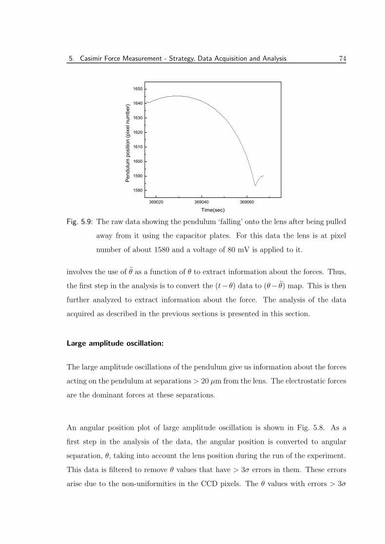
5. Casimir Force Measurement - Strategy, Data Acquisition and Analysis 74
369020 369040 369060
1580
1590
1600
1610
1620
1630
1640
1650
Pend
ulum
pos
ition
(pix
el n
umbe
r)
Time(sec)
Fig. 5.9: The raw data showing the pendulum ‘falling’ onto the lens after being pulled
away from it using the capacitor plates. For this data the lens is at pixel
number of about 1580 and a voltage of 80 mV is applied to it.
involves the use of θ as a function of θ to extract information about the forces. Thus,
the first step in the analysis is to convert the (t−θ) data to (θ− θ) map. This is then
further analyzed to extract information about the force. The analysis of the data
acquired as described in the previous sections is presented in this section.
Large amplitude oscillation:
The large amplitude oscillations of the pendulum give us information about the forces
acting on the pendulum at separations > 20 µm from the lens. The electrostatic forces
are the dominant forces at these separations.
An angular position plot of large amplitude oscillation is shown in Fig. 5.8. As a
first step in the analysis of the data, the angular position is converted to angular
separation, θ, taking into account the lens position during the run of the experiment.
This data is filtered to remove θ values that have > 3σ errors in them. These errors
arise due to the non-uniformities in the CCD pixels. The θ values with errors > 3σ
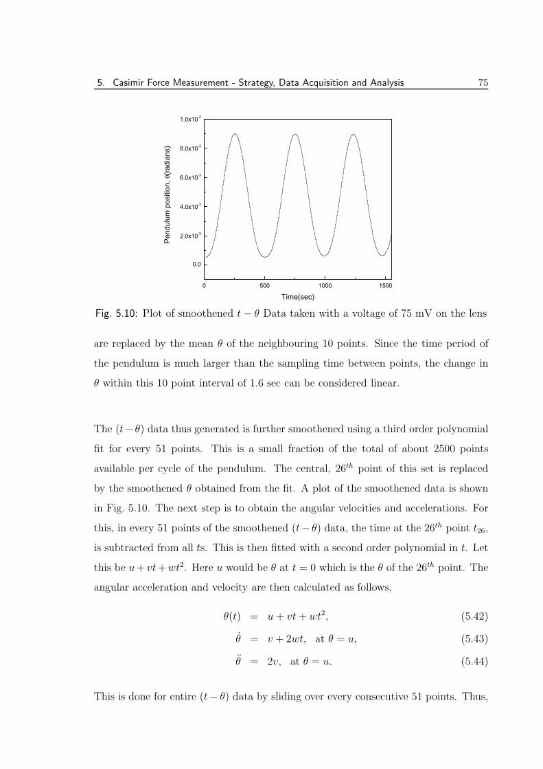
5. Casimir Force Measurement - Strategy, Data Acquisition and Analysis 75
0 500 1000 1500
0.0
2.0x10⁻³
4.0x10⁻³
6.0x10⁻³
8.0x10⁻³
1.0x10⁻²
Pend
ulum
pos
ition
, (ra
dian
s)
Time(sec)
Fig. 5.10: Plot of smoothened t− θ Data taken with a voltage of 75 mV on the lens
are replaced by the mean θ of the neighbouring 10 points. Since the time period of
the pendulum is much larger than the sampling time between points, the change in
θ within this 10 point interval of 1.6 sec can be considered linear.
The (t−θ) data thus generated is further smoothened using a third order polynomial
fit for every 51 points. This is a small fraction of the total of about 2500 points
available per cycle of the pendulum. The central, 26th point of this set is replaced
by the smoothened θ obtained from the fit. A plot of the smoothened data is shown
in Fig. 5.10. The next step is to obtain the angular velocities and accelerations. For
this, in every 51 points of the smoothened (t− θ) data, the time at the 26th point t26,
is subtracted from all ts. This is then fitted with a second order polynomial in t. Let
this be u+ vt+wt2. Here u would be θ at t = 0 which is the θ of the 26th point. The
angular acceleration and velocity are then calculated as follows,
θ(t) = u+ vt+ wt2, (5.42)
θ = v + 2wt, at θ = u, (5.43)
θ = 2v, at θ = u. (5.44)
This is done for entire (t− θ) data by sliding over every consecutive 51 points. Thus,
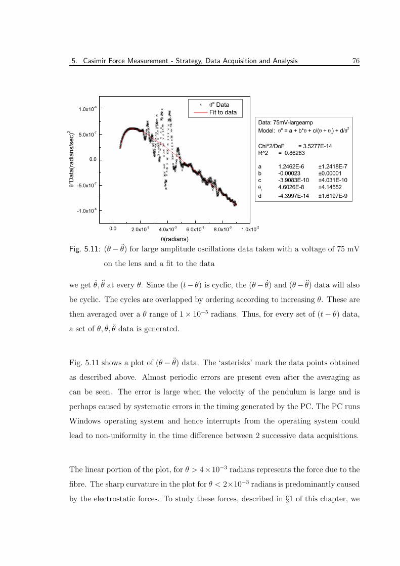
5. Casimir Force Measurement - Strategy, Data Acquisition and Analysis 76
0.0 2.0x10⁻³ 4.0x10⁻³ 6.0x10⁻³ 8.0x10⁻³ 1.0x10⁻²
-1.0x10⁻⁶
-5.0x10⁻⁷
0.0
5.0x10⁻⁷
1.0x10⁻⁶ " Data Fit to data
Data: 75mV-largeampModel: " = a + b* + c/( + r) + d/ 2
Chi^2/DoF = 3.5277E-14R^2 = 0.86283 a 1.2462E-6 ±1.2418E-7b -0.00023 ±0.00001c -3.9083E-10 ±4.031E-10
r 4.6026E-8 ±4.14552d -4.3997E-14 ±1.6197E-9
"Dat
a(ra
dian
s/se
c)2
(radians)Fig. 5.11: (θ− θ) for large amplitude oscillations data taken with a voltage of 75 mV
on the lens and a fit to the data
we get θ, θ at every θ. Since the (t− θ) is cyclic, the (θ− θ) and (θ− θ) data will also
be cyclic. The cycles are overlapped by ordering according to increasing θ. These are
then averaged over a θ range of 1× 10⁻⁵ radians. Thus, for every set of (t− θ) data,
a set of θ, θ, θ data is generated.
Fig. 5.11 shows a plot of (θ− θ) data. The ‘asterisks’ mark the data points obtained
as described above. Almost periodic errors are present even after the averaging as
can be seen. The error is large when the velocity of the pendulum is large and is
perhaps caused by systematic errors in the timing generated by the PC. The PC runs
Windows operating system and hence interrupts from the operating system could
lead to non-uniformity in the time difference between 2 successive data acquisitions.
The linear portion of the plot, for θ > 4×10⁻³ radians represents the force due to the
fibre. The sharp curvature in the plot for θ < 2×10⁻³ radians is predominantly caused
by the electrostatic forces. To study these forces, described in §1 of this chapter, we
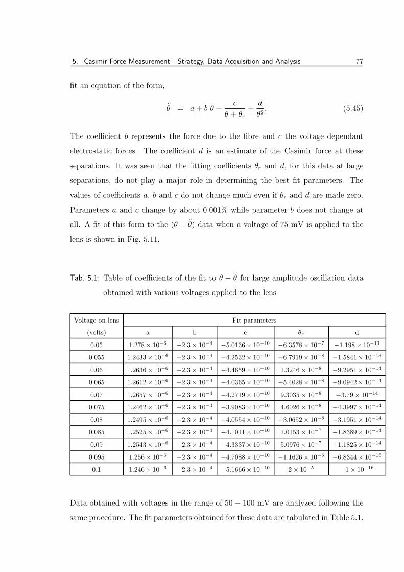
5. Casimir Force Measurement - Strategy, Data Acquisition and Analysis 77
fit an equation of the form,
θ = a + b θ +c
θ + θr+
d
θ2. (5.45)
The coefficient b represents the force due to the fibre and c the voltage dependant
electrostatic forces. The coefficient d is an estimate of the Casimir force at these
separations. It was seen that the fitting coefficients θr and d, for this data at large
separations, do not play a major role in determining the best fit parameters. The
values of coefficients a, b and c do not change much even if θr and d are made zero.
Parameters a and c change by about 0.001% while parameter b does not change at
all. A fit of this form to the (θ − θ) data when a voltage of 75 mV is applied to the
lens is shown in Fig. 5.11.
Tab. 5.1: Table of coefficients of the fit to θ − θ for large amplitude oscillation data
obtained with various voltages applied to the lens
Voltage on lens Fit parameters
(volts) a b c θr d
0.05 1.278× 10⁻⁶ −2.3× 10⁻⁴ −5.0136× 10⁻¹⁰ −6.3578× 10⁻⁷ −1.198× 10⁻¹³
0.055 1.2433× 10⁻⁶ −2.3× 10⁻⁴ −4.2532× 10⁻¹⁰ −6.7919× 10⁻⁸ −1.5841× 10⁻¹³
0.06 1.2636× 10⁻⁶ −2.3× 10⁻⁴ −4.4659× 10⁻¹⁰ 1.3246× 10⁻⁸ −9.2951× 10⁻¹⁴
0.065 1.2612× 10⁻⁶ −2.3× 10⁻⁴ −4.0365× 10⁻¹⁰ −5.4028× 10⁻⁸ −9.0942× 10⁻¹⁴
0.07 1.2657× 10⁻⁶ −2.3× 10⁻⁴ −4.2719× 10⁻¹⁰ 9.3035× 10⁻⁸ −3.79× 10⁻¹⁴
0.075 1.2462× 10⁻⁶ −2.3× 10⁻⁴ −3.9083× 10⁻¹⁰ 4.6026× 10⁻⁸ −4.3997× 10⁻¹⁴
0.08 1.2495× 10⁻⁶ −2.3× 10⁻⁴ −4.0554× 10⁻¹⁰ −3.0652× 10⁻⁸ −3.1951× 10⁻¹⁴
0.085 1.2525× 10⁻⁶ −2.3× 10⁻⁴ −4.1011× 10⁻¹⁰ 1.0153× 10⁻⁷ −1.8389× 10⁻¹⁴
0.09 1.2543× 10⁻⁶ −2.3× 10⁻⁴ −4.3337× 10⁻¹⁰ 5.0976× 10⁻⁷ −1.1825× 10⁻¹⁴
0.095 1.256× 10⁻⁶ −2.3× 10⁻⁴ −4.7088× 10⁻¹⁰ −1.1626× 10⁻⁶ −6.8344× 10⁻¹⁵
0.1 1.246× 10⁻⁶ −2.3× 10⁻⁴ −5.1666× 10⁻¹⁰ 2× 10⁻⁵ −1× 10⁻¹⁶
Data obtained with voltages in the range of 50− 100 mV are analyzed following the
same procedure. The fit parameters obtained for these data are tabulated in Table 5.1.
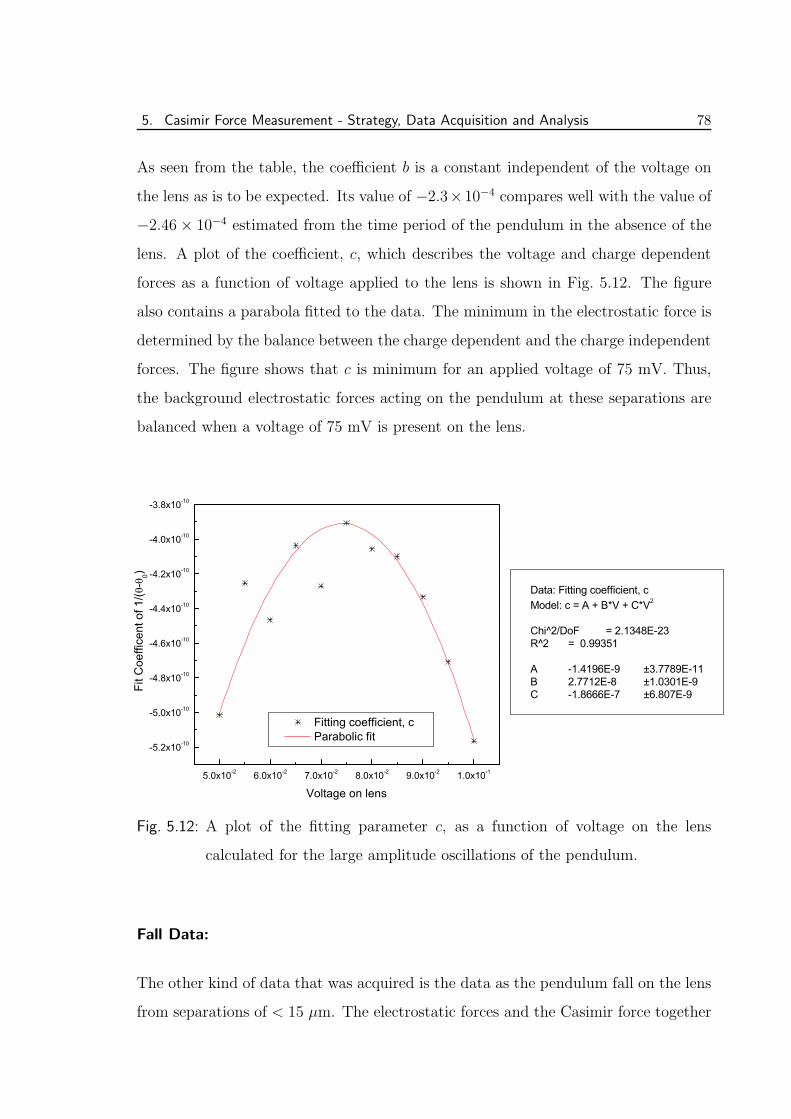
5. Casimir Force Measurement - Strategy, Data Acquisition and Analysis 78
As seen from the table, the coefficient b is a constant independent of the voltage on
the lens as is to be expected. Its value of −2.3×10⁻⁴ compares well with the value of
−2.46 × 10⁻⁴ estimated from the time period of the pendulum in the absence of the
lens. A plot of the coefficient, c, which describes the voltage and charge dependent
forces as a function of voltage applied to the lens is shown in Fig. 5.12. The figure
also contains a parabola fitted to the data. The minimum in the electrostatic force is
determined by the balance between the charge dependent and the charge independent
forces. The figure shows that c is minimum for an applied voltage of 75 mV. Thus,
the background electrostatic forces acting on the pendulum at these separations are
balanced when a voltage of 75 mV is present on the lens.
5.0x10⁻² 6.0x10⁻² 7.0x10⁻² 8.0x10⁻² 9.0x10⁻² 1.0x10⁻¹
-5.2x10⁻¹⁰
-5.0x10⁻¹⁰
-4.8x10⁻¹⁰
-4.6x10⁻¹⁰
-4.4x10⁻¹⁰
-4.2x10⁻¹⁰
-4.0x10⁻¹⁰
-3.8x10⁻¹⁰
Fitting coefficient, c Parabolic fit
Data: Fitting coefficient, cModel: c = A + B*V + C*V2
Chi^2/DoF = 2.1348E-23R^2 = 0.99351 A -1.4196E-9 ±3.7789E-11B 2.7712E-8 ±1.0301E-9C -1.8666E-7 ±6.807E-9Fi
t Coe
ffice
nt o
f 1/(
-0)
Voltage on lens
Fig. 5.12: A plot of the fitting parameter c, as a function of voltage on the lens
calculated for the large amplitude oscillations of the pendulum.
Fall Data:
The other kind of data that was acquired is the data as the pendulum fall on the lens
from separations of < 15 µm. The electrostatic forces and the Casimir force together
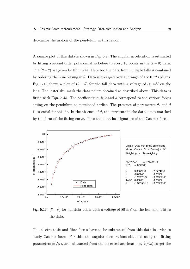
5. Casimir Force Measurement - Strategy, Data Acquisition and Analysis 79
determine the motion of the pendulum in this region.
A sample plot of this data is shown in Fig. 5.9. The angular acceleration is estimated
by fitting a second order polynomial as before to every 10 points in the (t− θ) data.
The (θ− θ) are given by Eqn. 5.44. Here too the data from multiple falls is combined
by ordering them increasing in θ. Data is averaged over a θ range of 1×10⁻⁵ radians.
Fig. 5.13 shows a plot of (θ − θ) for the fall data with a voltage of 80 mV on the
lens. The ‘asterisks’ mark the data points obtained as described above. This data is
fitted with Eqn. 5.45. The coefficients a, b, c and d correspond to the various forces
acting on the pendulum as mentioned earlier. The presence of parameters θr and d
is essential for this fit. In the absence of d, the curvature in the data is not matched
by the form of the fitting curve. Thus this data has signature of the Casimir force.
0.0 1.0x10⁻⁴ 2.0x10⁻⁴ 3.0x10⁻⁴ 4.0x10⁻⁴-8.0x10⁻⁶
-7.0x10⁻⁶
-6.0x10⁻⁶
-5.0x10⁻⁶
-4.0x10⁻⁶
-3.0x10⁻⁶
-2.0x10⁻⁶
-1.0x10⁻⁶
0.0
Data: " Data with 80mV on the lensModel: " = a + b* + c/( + r) + d/ 2
Weighting: y No weighting Chi^2/DoF = 1.2746E-14R^2 = 0.99588 a 3.3882E-6 ±2.5474E-6b -0.00245 ±0.00307c -1.2802E-9 ±9.0135E-10theta0 0.00013 ±0.00007d -1.3015E-15 ±3.7535E-16
" (ra
dian
s/se
c)2
(radians)
Data Fit to data
Fig. 5.13: (θ − θ) for fall data taken with a voltage of 80 mV on the lens and a fit to
the data.
The electrostatic and fibre forces have to be subtracted from this data in order to
study Casimir force. For this, the angular accelerations obtained using the fitting
parameters θ(fit), are subtracted from the observed accelerations, θ(obs) to get the
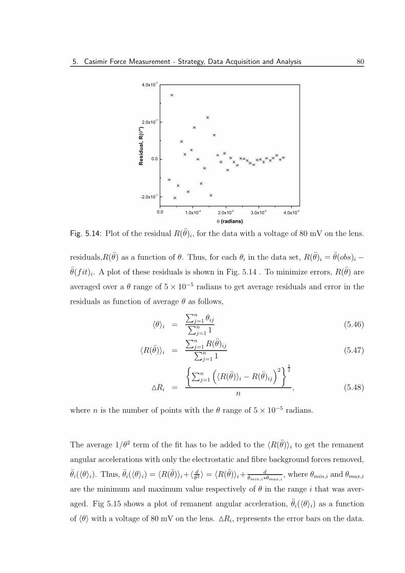
5. Casimir Force Measurement - Strategy, Data Acquisition and Analysis 80
0.0 1.0x10⁻⁴ 2.0x10⁻⁴ 3.0x10⁻⁴ 4.0x10⁻⁴
-2.0x10⁻⁷
0.0
2.0x10⁻⁷
4.0x10⁻⁷
Res
idua
l, R
(")
(radians)
Fig. 5.14: Plot of the residual R(θ)i, for the data with a voltage of 80 mV on the lens.
residuals,R(θ) as a function of θ. Thus, for each θi in the data set, R(θ)i = θ(obs)i −θ(fit)i. A plot of these residuals is shown in Fig. 5.14 . To minimize errors, R(θ) are
averaged over a θ range of 5× 10⁻⁵ radians to get average residuals and error in the
residuals as function of average θ as follows,
〈θ〉i =
∑nj=1 θij∑n
j=1 1(5.46)
〈R(θ)〉i =
∑nj=1R(θ)ij∑n
j=1 1(5.47)
△Ri =
{
∑nj=1
(
〈R(θ)〉i − R(θ)ij
)2}
1
2
n, (5.48)
where n is the number of points with the θ range of 5× 10⁻⁵ radians.
The average 1/θ2 term of the fit has to be added to the 〈R(θ)〉i to get the remanent
angular accelerations with only the electrostatic and fibre background forces removed,
θi(〈θ〉i). Thus, θi(〈θ〉i) = 〈R(θ)〉i+〈 dθ2〉 = 〈R(θ)〉i+ d
θmin,i∗θmax,i, where θmin,i and θmax,i
are the minimum and maximum value respectively of θ in the range i that was aver-
aged. Fig 5.15 shows a plot of remanent angular acceleration, θi(〈θ〉i) as a function
of 〈θ〉 with a voltage of 80 mV on the lens. △Ri, represents the error bars on the data.
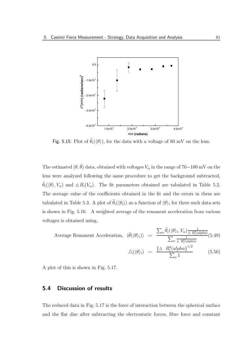
5. Casimir Force Measurement - Strategy, Data Acquisition and Analysis 81
1.0x10⁻⁴ 2.0x10⁻⁴ 3.0x10⁻⁴ 4.0x10⁻⁴-4.0x10⁻⁷
-3.0x10⁻⁷
-2.0x10⁻⁷
-1.0x10⁻⁷
0.0
"(<
>) (r
adia
ns/s
ec)2
< > (radians)
Fig. 5.15: Plot of θi(〈θ〉), for the data with a voltage of 80 mV on the lens.
The estimated (θ, θ) data, obtained with voltages Vα in the range of 70−100 mV on the
lens were analyzed following the same procedure to get the background subtracted,
θi(〈θ〉, Vα) and △Ri(Vα). The fit parameters obtained are tabulated in Table 5.2.
The average value of the coefficients obtained in the fit and the errors in them are
tabulated in Table 5.3. A plot of θi(〈θi〉) as a function of 〈θ〉i for three such data sets
is shown in Fig. 5.16. A weighted average of the remanent acceleration from various
voltages is obtained using,
Average Remanent Acceleration, 〈θ(〈θ〉i)〉 =
∑
α θi(〈θ〉i, Vα)1
△ R2
i (alpha)∑
α1
△ R2
i (alpha)
(5.49)
△(〈θ〉i) ={△ R2
i (alpha}1/2
∑
α 1(5.50)
A plot of this is shown in Fig. 5.17.
5.4 Discussion of results
The reduced data in Fig. 5.17 is the force of interaction between the spherical surface
and the flat disc after subtracting the electrostatic forces, fibre force and constant
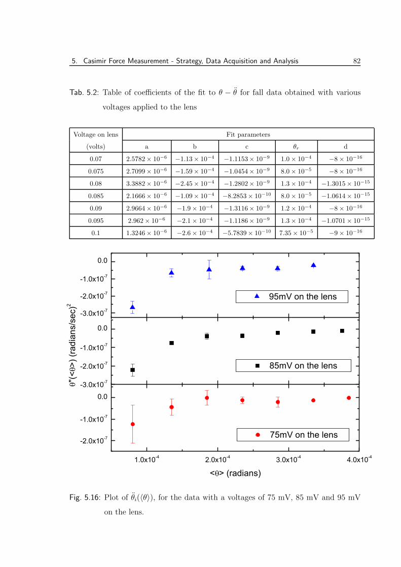
5. Casimir Force Measurement - Strategy, Data Acquisition and Analysis 82
Tab. 5.2: Table of coefficients of the fit to θ − θ for fall data obtained with various
voltages applied to the lens
Voltage on lens Fit parameters
(volts) a b c θr d
0.07 2.5782× 10⁻⁶ −1.13× 10⁻⁴ −1.1153× 10⁻⁹ 1.0× 10⁻⁴ −8× 10⁻¹⁶
0.075 2.7099× 10⁻⁶ −1.59× 10⁻⁴ −1.0454× 10⁻⁹ 8.0× 10⁻⁵ −8× 10⁻¹⁶
0.08 3.3882× 10⁻⁶ −2.45× 10⁻⁴ −1.2802× 10⁻⁹ 1.3× 10⁻⁴ −1.3015× 10⁻¹⁵
0.085 2.1666× 10⁻⁶ −1.09× 10⁻⁴ −8.2853× 10⁻¹⁰ 8.0× 10⁻⁵ −1.0614× 10⁻¹⁵
0.09 2.9664× 10⁻⁶ −1.9× 10⁻⁴ −1.3116× 10⁻⁹ 1.2× 10⁻⁴ −8× 10⁻¹⁶
0.095 2.962× 10⁻⁶ −2.1× 10⁻⁴ −1.1186× 10⁻⁹ 1.3× 10⁻⁴ −1.0701× 10⁻¹⁵
0.1 1.3246× 10⁻⁶ −2.6× 10⁻⁴ −5.7839× 10⁻¹⁰ 7.35× 10⁻⁵ −9× 10⁻¹⁶
1.0x10⁻⁴ 2.0x10⁻⁴ 3.0x10⁻⁴ 4.0x10⁻⁴
-2.0x10⁻⁷
-1.0x10⁻⁷
0.0-3.0x10⁻⁷
-2.0x10⁻⁷
-1.0x10⁻⁷
0.0
-3.0x10⁻⁷
-2.0x10⁻⁷
-1.0x10⁻⁷
0.0
75mV on the lens
"(<
>) (r
adia
ns/s
ec)2
< > (radians)
85mV on the lens
95mV on the lens
Fig. 5.16: Plot of θi(〈θ〉), for the data with a voltages of 75 mV, 85 mV and 95 mV
on the lens.
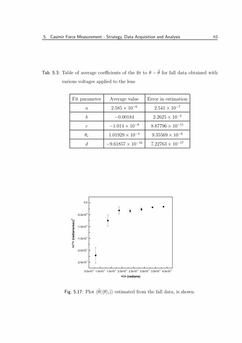
5. Casimir Force Measurement - Strategy, Data Acquisition and Analysis 83
Tab. 5.3: Table of average coefficients of the fit to θ − θ for fall data obtained with
various voltages applied to the lens
Fit parameter Average value Error in estimation
a 2.585× 10⁻⁶ 2.541× 10⁻⁷
b −0.00184 2.2625× 10⁻⁴
c −1.014× 10⁻⁹ 8.87796× 10⁻¹¹
θr 1.01929× 10⁻⁴ 9.35569× 10⁻⁶
d −9.61857× 10⁻¹⁶ 7.22763× 10⁻¹⁷
5.0x10⁻⁵ 1.0x10⁻⁴ 1.5x10⁻⁴ 2.0x10⁻⁴ 2.5x10⁻⁴ 3.0x10⁻⁴ 3.5x10⁻⁴ 4.0x10⁻⁴
-2.5x10⁻⁷
-2.0x10⁻⁷
-1.5x10⁻⁷
-1.0x10⁻⁷
-5.0x10⁻⁸
0.0
<">
(rad
ians
/sec
)2
< > (radians)
Fig. 5.17: Plot 〈θ(〈θ〉i)〉 estimated from the fall data, is shown.
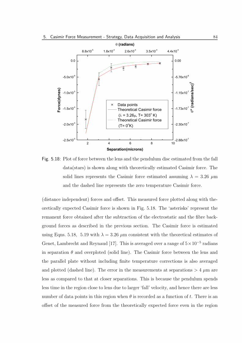
5. Casimir Force Measurement - Strategy, Data Acquisition and Analysis 84
2 4 6 8 10-2.5x10⁻⁵
-2.0x10⁻⁵
-1.5x10⁻⁵
-1.0x10⁻⁵
-5.0x10⁻⁶
0.0
8.8x10⁻⁵ 1.8x10⁻⁴ 2.6x10⁻⁴ 3.5x10⁻⁴ 4.4x10⁻⁴
-2.88x10⁻⁷
-2.30x10⁻⁷
-1.73x10⁻⁷
-1.15x10⁻⁷
-5.76x10⁻⁸
0.00
"
(rad
ians
/sec
)2
(radians)
Forc
e(dy
nes)
Separation(microns)
Data points Theoretical Casimir force
( = 3.26 , T= 303o K) Theoretical Casimir force
(T= 0oK)
Fig. 5.18: Plot of force between the lens and the pendulum disc estimated from the fall
data(stars) is shown along with theoretically estimated Casimir force. The
solid lines represents the Casimir force estimated assuming λ = 3.26 µm
and the dashed line represents the zero temperature Casimir force.
(distance independent) forces and offset. This measured force plotted along with the-
oretically expected Casimir force is shown in Fig. 5.18. The ‘asterisks’ represent the
remanent force obtained after the subtraction of the electrostatic and the fibre back-
ground forces as described in the previous section. The Casimir force is estimated
using Eqns. 5.18, 5.19 with λ = 3.26 µm consistent with the theoretical estimates of
Genet, Lambrecht and Reynaud [17]. This is averaged over a range of 5×10⁻⁵ radians
in separation θ and overploted (solid line). The Casimir force between the lens and
the parallel plate without including finite temperature corrections is also averaged
and plotted (dashed line). The error in the measurements at separations > 4 µm are
less as compared to that at closer separations. This is because the pendulum spends
less time in the region close to lens due to larger ‘fall’ velocity, and hence there are less
number of data points in this region when θ is recorded as a function of t. There is an
offset of the measured force from the theoretically expected force even in the region
References 85
where the errors are small. This offset is a small fraction of the error on the constant
term ‘a’ in the fit, Eqn.5.45, to the entire data. If the data is normalized to the
finite temperature Casimir force at 9 µm by adding a constant offset to all the data
points, the measured force agrees with the theoretically calculated finite temperature
Casimir force within the statistical errors of the data. The required offset of 8.4×10⁻⁹
(radians/sec)2 or 3.61 × 10⁻⁷ dynes is ∼ 1/30th of the error in the estimation of the
constant coefficient from the fit, which is 2.541×10⁻⁷ (radians/sec)2 [Table 5.1]. Also
this offset is of the order of the expected residual gravitational force on the pendulum
due to the lens [see §5.1.1]. The deviation of the data from the finite temperature
Casimir force around separations of 4 µm is due to the fact that we have imposed a
strict cut-off for the change over from zero temperature to finite temperature theory
at λ = 3.26 µm. The actual force will gradually change from the dependance of 1/z2
to 1/z3 around z = 3.26 µm. Also there will be about 10% reduction in the estimated
Casimir force through out the range due to finite conductivity corrections.
Thus, the measured force is consonant with the presence of a force that is ∼ 1/z2,
viz., finite temperature Casimir force.
References
[1] E. G. Adelberger, B. R. Heckel, and A. E. Nelson. Tests of the Gravitational
Inverse-Square Law. ArXiv High Energy Physics - Phenomenology e-prints, July
2003.
[2] J. Blocki et al. . Ann. Phys. (N.Y.), 105:427, 1977.
[3] G. Bressi et al. Measurement of the Casimir Force between Parallel Metallic
Surfaces. Phys. Rev. Lett, 88:041804–1, 2002.
[4] H. B. Chan et al. Quantum Mechanical Actuation of Micromechanical Systems
by the Casimir Force. Science, 291:9, 2001.
References 86
[5] B. V Derjaguin. The Force Between Molecules. Sci. Am., 203:47, 1960.
[6] B. V Derjaguin and J. J. Abrikossova. Disc. Faraday Soc., 18:33, 1954.
[7] C. Genet, A. Lambrecht, and S. Reynaud. Temperature dependence of the
Casimir effect between metallic mirrors. Phy.Rev. A, 62:012110, July 2000.
[8] S. K. Lamoreaux. Demonstration of the Casimir Force in the 0.6 to 6 µ Range.
Phys. Rev. Lett, 78:5, 1997.
[9] U. Mohideen and A Roy. Precision Measurement of the Casimir Force from 0.1
to 0.9 µm Range. Phys. Rev. Lett, 81:4549, 1998.
[10] W. R Smythe. Static and Dynamic Electricity. McGraw Hill, 1939.
[11] M. J. Sparnaay. Attractive Forces Between Flat Plates. Nature, 180:334, 1957.
[12] C. C. Speake. Forces and force gradients due to patch fields and contact-potential
differences. Classical and Quantum Gravity, 13:291–, November 1996.
[13] C. C. Speake and C. Trenkel. Forces between Conducting Surfaces due to Spatial
Variations of Surface Potential. Physical Review Letters, 90:160403, 2003.
[14] P. H. G. M van Blokland and J. T. G. Overbeek. van der Waals Forces Be-
tween Objects Covered with Chromium Layer. J. Chem. Soc. Faraday Trans.
72, 72:2637, 1978.
6. COMPARISON OF EXPERIMENTS ON
CASIMIR FORCE
Abstract: A brief review of various experiments performed to study the Casimir effect
will be presented. We then compare the results from the recent experiments with our
results. The first ever detection and measurement of finite temperature corrections to
Casimir force in our experiment is highlighted.
6.1 Experiments to Study Casimir force
Experimental studies on Casimir force started half a century ago, a few years after
Casimir predicted the existence of the force in 1948 [3]. A historical overview of
the experiments was presented in the first chapter. Extensive reviews may be found
in [4, 5]. We now discuss the details about some of the pioneering experiments mea-
suring Casimir force.
Overbeek and Sparnaay [15] were the first to attempt to measure the Casimir force.
They tried to measure the force between two parallel polished flat glass plates with
a surface area of 1 cm2, in the distance range of 0.6 µm to 1.5 µm. The distance
was sometimes made 0.2 µm. The force was measured using a spring balance. The
displacement of the spring was measured by means of a capacitive method. The mea-
surements at 1.2 µm, ‘pointed to the existence of a force which were of the expected
order of magnitude’ [17]. The hygroscopic behaviour of the glass (quartz) surfaces
and presence of dust particles presented difficulties.
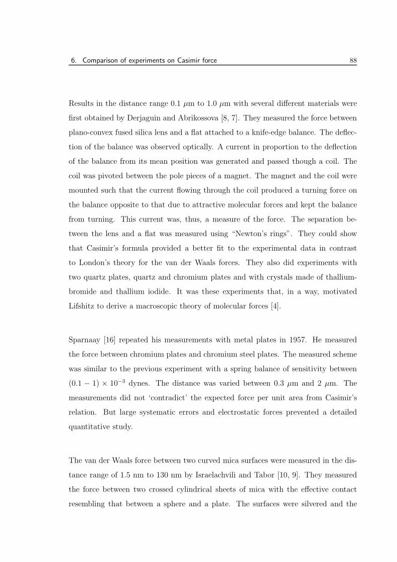
6. Comparison of experiments on Casimir force 88
Results in the distance range 0.1 µm to 1.0 µm with several different materials were
first obtained by Derjaguin and Abrikossova [8, 7]. They measured the force between
plano-convex fused silica lens and a flat attached to a knife-edge balance. The deflec-
tion of the balance was observed optically. A current in proportion to the deflection
of the balance from its mean position was generated and passed though a coil. The
coil was pivoted between the pole pieces of a magnet. The magnet and the coil were
mounted such that the current flowing through the coil produced a turning force on
the balance opposite to that due to attractive molecular forces and kept the balance
from turning. This current was, thus, a measure of the force. The separation be-
tween the lens and a flat was measured using “Newton’s rings”. They could show
that Casimir’s formula provided a better fit to the experimental data in contrast
to London’s theory for the van der Waals forces. They also did experiments with
two quartz plates, quartz and chromium plates and with crystals made of thallium-
bromide and thallium iodide. It was these experiments that, in a way, motivated
Lifshitz to derive a macroscopic theory of molecular forces [4].
Sparnaay [16] repeated his measurements with metal plates in 1957. He measured
the force between chromium plates and chromium steel plates. The measured scheme
was similar to the previous experiment with a spring balance of sensitivity between
(0.1 − 1) × 10−3 dynes. The distance was varied between 0.3 µm and 2 µm. The
measurements did not ‘contradict’ the expected force per unit area from Casimir’s
relation. But large systematic errors and electrostatic forces prevented a detailed
quantitative study.
The van der Waals force between two curved mica surfaces were measured in the dis-
tance range of 1.5 nm to 130 nm by Israelachvili and Tabor [10, 9]. They measured
the force between two crossed cylindrical sheets of mica with the effective contact
resembling that between a sphere and a plate. The surfaces were silvered and the
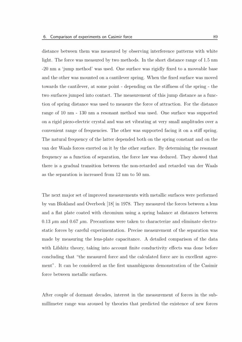
6. Comparison of experiments on Casimir force 89
distance between them was measured by observing interference patterns with white
light. The force was measured by two methods. In the short distance range of 1.5 nm
-20 nm a ‘jump method’ was used. One surface was rigidly fixed to a moveable base
and the other was mounted on a cantilever spring. When the fixed surface was moved
towards the cantilever, at some point - depending on the stiffness of the spring - the
two surfaces jumped into contact. The measurement of this jump distance as a func-
tion of spring distance was used to measure the force of attraction. For the distance
range of 10 nm - 130 nm a resonant method was used. One surface was supported
on a rigid piezo-electric crystal and was set vibrating at very small amplitudes over a
convenient range of frequencies. The other was supported facing it on a stiff spring.
The natural frequency of the latter depended both on the spring constant and on the
van der Waals forces exerted on it by the other surface. By determining the resonant
frequency as a function of separation, the force law was deduced. They showed that
there is a gradual transition between the non-retarded and retarded van der Waals
as the separation is increased from 12 nm to 50 nm.
The next major set of improved measurements with metallic surfaces were performed
by van Blokland and Overbeek [18] in 1978. They measured the forces between a lens
and a flat plate coated with chromium using a spring balance at distances between
0.13 µm and 0.67 µm. Precautions were taken to characterize and eliminate electro-
static forces by careful experimentation. Precise measurement of the separation was
made by measuring the lens-plate capacitance. A detailed comparison of the data
with Lifshitz theory, taking into account finite conductivity effects was done before
concluding that “the measured force and the calculated force are in excellent agree-
ment”. It can be considered as the first unambiguous demonstration of the Casimir
force between metallic surfaces.
After couple of dormant decades, interest in the measurement of forces in the sub-
millimeter range was aroused by theories that predicted the existence of new forces
6. Comparison of experiments on Casimir force 90
in this range. The earliest of these experiments was by Lamoreaux in 1997 [24] and
around the same time we started the design of our experiment [5]. The apparatus
built by Lamoreaux consists of a glass plate coated with gold over copper suspended
as a torsional pendulum. Its attraction towards a spherical lens also coated with
copper and gold was measured for distances between 0.6 µm - 6 µm. The plate was
held fixed with respect to the spherical surface by a voltage applied to two compen-
sating capacitor plates held parallel to the ‘Casimir’ plate. By measuring the change
in the voltage required to hold the plates parallel when the lens was moved towards
the ‘Casimir’ plate, the Casimir force was measured. He detected and corrected for a
contact potential between the lens and the plate of 250 mV. The measured Casimir
force agreed with theory at the level of 5% up to separation of about 2 µm. The sen-
sitivity of the experiment was not adequate to measure the force beyond this range.
In a later experiment, Mohideen and Roy [14] measured the Casimir force between
a metallized sphere of diameter 196 µm and a flat plate for separations from 0.1 to
0.9 µm. They used the high sensitivity of an Atomic force microscope to report a
statistical precision of 1% at the smallest separations. The electrostatic force due a
residual voltage of 29 mV was measured and subtracted from the data.
A micromechanical actuator based on Casimir force was developed by researchers at
Bell Labs [4] in 2001. The device, fabricated using standard nanofabrication tech-
niques, consists of a 3.5 µm thick, 500 µm square heavily doped polysilicon plate
freely suspended on two opposite sides by thin torsional rods. The other ends of the
torsional rods were anchored to the substrate. There was a 2 µm gap between the
top plate and the underlying substrate. A gold coated ball was suspended above one
side of the plate, which caused the plate to tilt due to Casimir force when the plate
was brought close to the ball. This tilt was determined by measuring the capacitance
between the plate and the substrate accurately. A residual voltage of 30 mV was
determined and compensated for. The measurements matched with Casimir force
6. Comparison of experiments on Casimir force 91
theory at the 1% level. The errors were mainly due to the corrections for finite con-
ductivity and surface roughness that have to be applied to the theory.
Recently, Bressi et al. [2] have measured the Casimir force between parallel metallic
surfaces. This is the first and only precision measurement of the Casimir force in
the ‘parallel plate’ configuration. The force was exerted between a silicon cantilever
coated with chromium and a similar rigid surface and was detected by looking at
the shifts induced in the cantilever frequency when the latter was approached. The
motion of the cantilever was monitored by means of a fiber optic interferometer. Elec-
trostatic force due a residual voltage of ∼ −68 mV is systematically determined and
corrected for. The scaling of the Casimir force with the distance between the surfaces
was tested in the 0.5 µm - 3.0 µm range, and the related force coefficient was deter-
mined at the 15% precision level.
Very recently, the Casimir force between two dissimilar metals was measured by Decca
et al. [6] in the separation range of 0.52 µm - 2.0 µm. They measure the force of
attraction between a copper layer evaporated on a micro-mechanical torsional pendu-
lum and a gold layer deposited on an Aluminium oxide sphere with 600 µm nominal
diameter. The force is inferred from the deflection angle of the torsional oscillator
determined by measuring the capacitance between the oscillator and two fixed elec-
trodes. The sensitivity of the force measurement was further improved by measuring
the change in the resonant frequency of the oscillator due to the presence of the
sphere. Residual voltage difference of 632.5 mV was determined by experimentation
and corresponds to the difference in work functions of the gold and copper layers.
The experiment highlights the need for simultaneous measurement of the dielectric
constant of the metallic films used for a better understanding of the Casimir force
between non-ideal bodies at these separations.
6. Comparison of experiments on Casimir force 92
6.2 Comparison of results
The Casimir force has been measured over a wide range of separation from 1.5 nm to
3 µm by various techniques. Most experiments have been performed in the sphere-
plate geometry rather than in the plate-plate geometry due to stringent conditions of
parallelism required in the latter. All the experiments encountered a background of
strong electrostatic forces due to residual voltages present on the interacting bodies
even when these are well grounded. The Casimir force for the sphere-plate geometry,
depends on the radius of the sphere used and is typically much larger than the electro-
static force at sub-micron separations. But at larger separations, the measurements
are dominated by the electrostatic forces, making it difficult to perform experiments
in the several microns range. For example, an electrostatic contribution comparable
to the Casimir force at 1 µm becomes 10 times or more stronger than the finite tem-
perature Casimir force at 10 µm. The experiments performed thus far, have been
able to detect effects due to finite conductivity and surface roughness of the metals
on the Casimir force but the finite temperature correction has not been observed.
Our experiment measures the Casimir force in the separation range of 2 µm to 9 µm.
This region extends well into spacings beyond ∼ 3.3 µm where corrections to the
Casimir force due to the ∼ 300◦ K environment become significant. As expected,
the data clearly indicate the presence of the effects of finite temperature. Data from
recent experiments that measured the force in the sphere-plate configuration are sum-
marized in Fig. 6.1. The figure shows the force measured in these experiments divided
by 2πR, where R is the radius of curvature of sphere used in the respective experi-
ments. The results presented in this thesis are represented by the ‘stars’. The data
from various experiments overlap in the region where the errors are small. Our data,
below 3.3 µm overlaps well with the measurements by Lamoreaux. The slope of the
data represents the power of the force law obeyed by the data. Around separation
of ∼ 4 µm the plot distinctly shows the change in slope from ∼ −3 to ∼ −2 within
the errors of the experiments. There is a clear indication of the change-over in the
Casimir force law from the zero temperature theory to that due to finite temperature
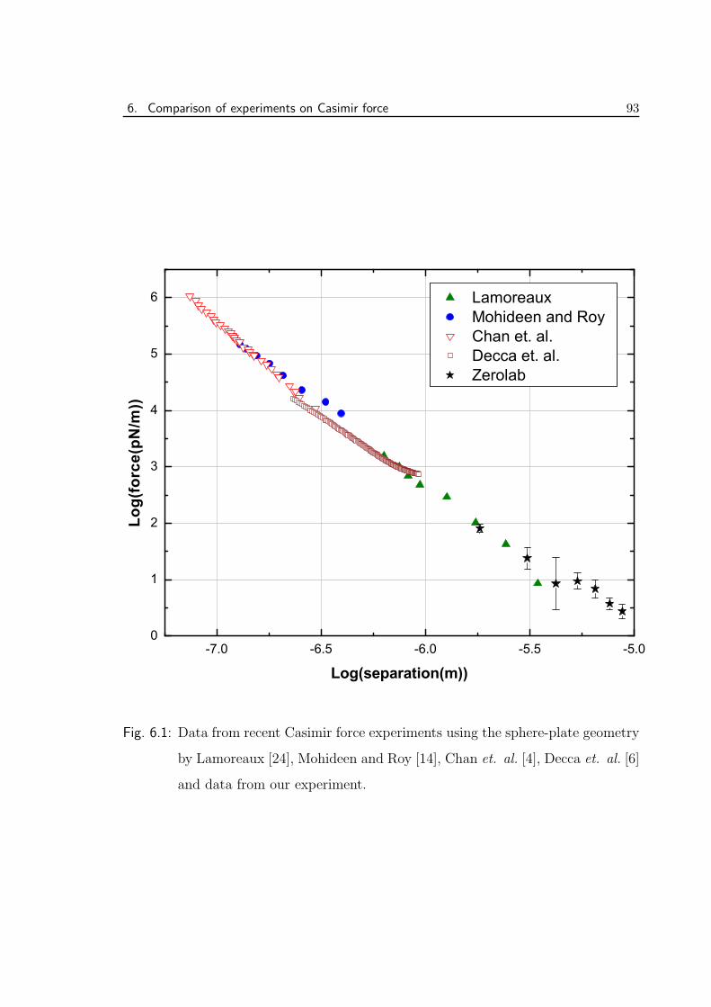
6. Comparison of experiments on Casimir force 93
-7.0 -6.5 -6.0 -5.5 -5.00
1
2
3
4
5
6 Lamoreaux Mohideen and Roy Chan et. al. Decca et. al. Zerolab
Log(force(pN
/m))
Log(separation(m))
Fig. 6.1: Data from recent Casimir force experiments using the sphere-plate geometry
by Lamoreaux [24], Mohideen and Roy [14], Chan et. al. [4], Decca et. al. [6]
and data from our experiment.
References 94
around this separation.
In summary, our current study extends the observation of the Casimir effect up to
separations of 9 µm, i.e., well into the region where finite temperature effects become
important. The experiment confirms the existence of these effects and agrees with
the standard theory at the 20% level.
Keeping in mind the wide-ranging importance of Casimir forces it would be useful to
conduct such studies with greater accuracy and also extend them to longer separations
of ∼ 50 µm or more.
References
[1] M. Bordag, U. Mohideen, and V. M. Mostepanenko. New Developements in
Casimir Force. Phys. Rep., 353:1, 2001.
[2] G. Bressi et al. Measurement of the Casimir Force between Parallel Metallic
Surfaces. Phys. Rev. Lett, 88:041804–1, 2002.
[3] H. B. Casimir. On the Attraction Between Two Perfectly Conducting Plates.
Proc. K. Ned. Akad. Wet., 51:793, 1948.
[4] H. B. Chan et al. Quantum Mechanical Actuation of Micromechanical Systems
by the Casimir Force. Science, 291:9, 2001.
[5] R. Cowsik, B. P. Das, N. Krishnan, G. Rajalakshmi, D. Suresh, and C. S. Un-
nikrishnan. High Sensitivity Measurement of Casimir Force and Observability
of Finite Temperature Effects. In Proceedings of the Eighth Marcell-Grossmann
Meeting on General Relativity, page 949. World Scientific, 1998.
[6] R. Decca, D. Lopez, E. Fischbach, and D. Krause. Measurement of the Casimir
Force between Dissimilar Metals. Phys. Rev. Lett., 91:050402, July 2003.
[7] B. V Derjaguin. The Force Between Molecules. Sci. Am., 203:47, 1960.
References 95
[8] B. V Derjaguin and J. J. Abrikossova. Disc. Faraday Soc., 18:33, 1954.
[9] Israelachvili and Tabor. The Measurement of van der Waals dispersion forces in
the range 1.5 to 130nm. Proc. R. Soc. Lond. A, 331:39–55, 1972.
[10] Israelachvili and Tabor. Van der Waals dispersion forces-Measurements for
curved mica surfaces separated by between 1.4 and 70 nm. Nature Physical
Science, 236:106, April 1972.
[11] S. K. Lamoreaux. Demonstration of the Casimir Force in the 0.6 to 6 µ Range.
Phys. Rev. Lett, 78:5, 1997.
[12] E. M. Lifshitz. Theory of molecular attraction between solids. Sov. Phys. JETP,
2:73, 1956.
[13] W. P Milonni. The Quantum Vacuum: An Introduction to Quantum Electrody-
namics. Academic Press, Newyork, 1994.
[14] U. Mohideen and A Roy. Precision Measurement of the Casimir Force from 0.1
t0 0.9 µm Range. Phys. Rev. Lett, 81:4549, 1998.
[15] J. T. G. Overbeek and M. J. Sparnaay. Proc. K. Ned. Akad. Wet., 54:387, 1952.
[16] M. J. Sparnaay. Attractive Forces Between Flat Plates. Nature, 180:334, 1957.
[17] M. J. Sparnaay. Historical Background of Casimir force. In A. Sarlemijn and
M. J. Sparnaay, editors, Physics in the Making, North-Holland, 1989. Elsevier
Science Publishers B V.
[18] P. H. G. M van Blokland and J. T. G. Overbeek. van der Waals Forces Be-
tween Objects Covered with Chromium Layer. J. Chem. Soc. Faraday Trans.
72, 72:2637, 1978.
7. BOUNDS ON THE STRENGTH OF NEW
MACROSCOPIC FORCES AND FUTURE
DIRECTIONS
Abstract: We briefly review the experimental bounds on the strength of inverse square
law violating short-range interactions. The contribution of our experiment in this
direction will be presented. The future scope of our experiment to test and constrain
the predictions of fundamental theories will be discussed.
7.1 Constraints on new macroscopic forces
Extensions of the Standard Model predict the existence of a variety of neutral light
bosons. The exchange of these will mediate forces that lead to deviations from the
inverse square law of gravity at distances related to the mass of the bosons. String
and M-theories that attempt to unify the fundamental forces close to the Planck scale
or the theories with large extra dimensions that attempt to overcome the “hierarchy
problem” by invoking unification of the fundamental forces at the TeV scale of electro-
weak symmetry breaking, predict variations from the inverse square law of gravity at
sub-millimeter distances. An overview of these effects was presented in Chapter 1. In
general, the new macroscopic forces can be described by an addition of a Yukawa type
potential term to the gravitational interaction between two point masses as given by,
V (r) = −GM1M2
r
(
1 + αe−rλ
)
(7.1)
7. Bounds on the Strength of New Macroscopic Forces and Future Directions 97
where α represents the coupling strength of the interaction and λ the range. A recent
review of the experimental and the theoretical status of the inverse square law tests
can be found in [1]. Given this form for the potential, constraints can be placed on
the parameter space of α− λ from experiments that study long-range interactions
7.1.1 Astrophysical Bounds
Astronomical tests provide the best constraint on the parameter α at distance scales
λ > 1 km. These are typically obtained from observation of the Keplerian orbits of
the planets and the satellites and looking for deviations from normal gravity. The
measurements of precession of the lunar orbit using Lunar Laser Ranging studies
provides very good constraints in the 108 m scale. Precession is expected due the
quadrupole field of the Earth, gravitational perturbations from the other planets in
the solar system and general relativistic effects. Presence of Yukawa type interactions,
will add to the precession and hence limits can be placed on α after accounting for the
expected sources of the precession. A summary of the constraints from astrophysical
data is reproduced from [1, 15] in Fig. 7.1. In the range λ < 1 m, these limits have
been surpassed by laboratory experiments [19, 22, 25]. Details on geophysical and
laboratory constraints in the range λ > 1 m can be found in [23, 27] and [5]-[11].
Astronomical data can also provide evidence for the presence of extra dimensions
[2]. The cooling rate of the supernovae will increase by the presence of the extra
dimensions because energy from the explosion will be radiated into these dimensions
as well. This would lead to the reduction in the number of neutrinos emitted from the
supernovae. SN 1987A data constrains the size of the extra dimensions to < 0.7 µm
when the number of extra dimensions is 2 [2, 12, 20, 21]. This does not imply
that experiments at sub-millimeter scales will not observe effects due to the new
dimensions. A single large dimension of size 1 mm with several much smaller extra
dimensions is still allowed.
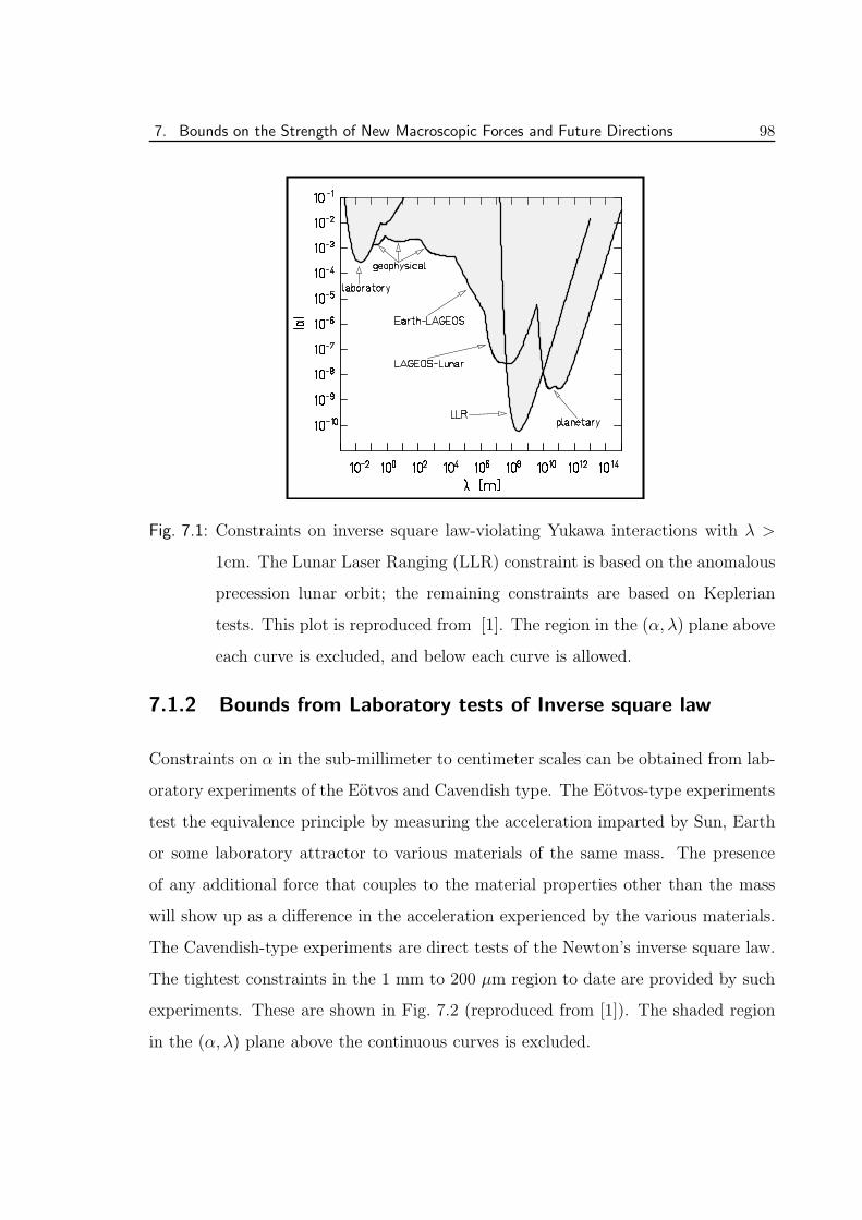
7. Bounds on the Strength of New Macroscopic Forces and Future Directions 98
Fig. 7.1: Constraints on inverse square law-violating Yukawa interactions with λ >
1cm. The Lunar Laser Ranging (LLR) constraint is based on the anomalous
precession lunar orbit; the remaining constraints are based on Keplerian
tests. This plot is reproduced from [1]. The region in the (α, λ) plane above
each curve is excluded, and below each curve is allowed.
7.1.2 Bounds from Laboratory tests of Inverse square law
Constraints on α in the sub-millimeter to centimeter scales can be obtained from lab-
oratory experiments of the Eotvos and Cavendish type. The Eotvos-type experiments
test the equivalence principle by measuring the acceleration imparted by Sun, Earth
or some laboratory attractor to various materials of the same mass. The presence
of any additional force that couples to the material properties other than the mass
will show up as a difference in the acceleration experienced by the various materials.
The Cavendish-type experiments are direct tests of the Newton’s inverse square law.
The tightest constraints in the 1 mm to 200 µm region to date are provided by such
experiments. These are shown in Fig. 7.2 (reproduced from [1]). The shaded region
in the (α, λ) plane above the continuous curves is excluded.
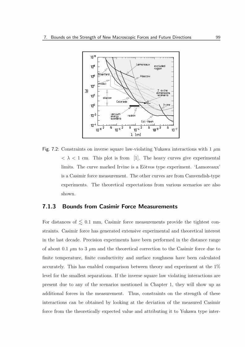
7. Bounds on the Strength of New Macroscopic Forces and Future Directions 99
Fig. 7.2: Constraints on inverse square law-violating Yukawa interactions with 1 µm
< λ < 1 cm. This plot is from [1]. The heavy curves give experimental
limits. The curve marked Irvine is a Eotvos type experiment. ‘Lamoreaux’
is a Casimir force measurement. The other curves are from Canvendish-type
experiments. The theoretical expectations from various scenarios are also
shown.
7.1.3 Bounds from Casimir Force Measurements
For distances of . 0.1 mm, Casimir force measurements provide the tightest con-
straints. Casimir force has generated extensive experimental and theoretical interest
in the last decade. Precision experiments have been performed in the distance range
of about 0.1 µm to 3 µm and the theoretical correction to the Casimir force due to
finite temperature, finite conductivity and surface roughness have been calculated
accurately. This has enabled comparison between theory and experiment at the 1%
level for the smallest separations. If the inverse square law violating interactions are
present due to any of the scenarios mentioned in Chapter 1, they will show up as
additional forces in the measurement. Thus, constraints on the strength of these
interactions can be obtained by looking at the deviation of the measured Casimir
force from the theoretically expected value and attributing it to Yukawa type inter-
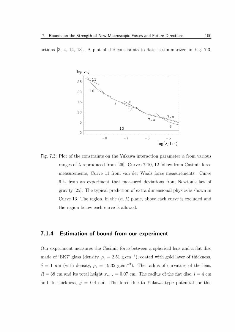
7. Bounds on the Strength of New Macroscopic Forces and Future Directions 100
actions [3, 4, 14, 13]. A plot of the constraints to date is summarized in Fig. 7.3.
-8 -7 -6 -5
0
5
10
15
20
25
6
7,a7,b
89
10
11
12
13 log(�=1m)
log j�Gj
Fig. 7.3: Plot of the constraints on the Yukawa interaction parameter α from various
ranges of λ reproduced from [26]. Curves 7-10, 12 follow from Casimir force
measurements, Curve 11 from van der Waals force measurements. Curve
6 is from an experiment that measured deviations from Newton’s law of
gravity [25]. The typical prediction of extra dimensional physics is shown in
Curve 13. The region, in the (α, λ) plane, above each curve is excluded and
the region below each curve is allowed.
7.1.4 Estimation of bound from our experiment
Our experiment measures the Casimir force between a spherical lens and a flat disc
made of ‘BK7’ glass (density, ρv = 2.51 g.cm−3), coated with gold layer of thickness,
δ = 1 µm (with density, ρs = 19.32 g.cm−3). The radius of curvature of the lens,
R = 38 cm and its total height xmax = 0.07 cm. The radius of the flat disc, l = 4 cm
and its thickness, g = 0.4 cm. The force due to Yukawa type potential for this
7. Bounds on the Strength of New Macroscopic Forces and Future Directions 101
configuration is given by (see Appendix C for details),
Fa(z) = 4π2GαRλ2[
ρs − (ρs − ρv)e−δ/λ
]
ρs δ e−z/λ, for λ << δ, (7.2)
Fb(z) = 4π2GαRλ2[
ρs − (ρs − ρv)e−δ/λ
] (
ρs δ + ρv λ e−δ/λ)
e−z/λ, (7.3)
for λ >> δ.
where α and λ are parameters of the theory as defined by Eqn. 7.1.
The upper limit of constraints on the Yukawa-type interactions from our experiments
can be estimated by two methods. A conservative estimate of the parameters of the
Yukawa-type interactions can be obtained by assuming that all of the force, fobs(z)
measured in our experiment is due to the Yukawa-type potential. Thus,
fobs(z) = F(z) (7.4)
We solve Eqn. 7.4 for the observed values of the force at z = 1.82 µm, 3.08 µm,
4.22 µm, 5.36 µm, 6.51 µm, 7.641 µm, 8.77 µm to get α as a function of λ, we call
this αconservative(λ). Since the thickness of the gold coatings, δ = 1 µm, we derive
αconservative(λ) in the range λ = 2 µm to 16 µm using Eqn. 7.3. This gives us seven
possible functions for αconservative(λ) corresponding to the seven separations at which
we have measurements. A plot of these is shown in Fig. 7.4. The lowest values of
αconservative(λ) are obtained from data at z = 8.77 µm in the range 7 µm ≤ λ ≤ 16 µm
and from data at z = 4.22 µm in the range 3 µm ≤ λ < 7 µm.
An optimistic estimate of the parameters of the Yukawa-type interactions can be
obtained from the error in the measurements of the force. Our experimental data
matches with the finite temperature Casimir force between the lens and the plate
within the errors of force measurement at separation z > 4 µm. The dominant con-
tribution to the finite temperature Casimir force for our configurations [see Appendix
A], at these separations is given by,
fcl(z) = −πRAc
λT
{
1
z2− 1
(z + xmax)2
}
, for z > λT = 3.26 µm; (7.5)
Ac =π2~c
240= 0.013× 10⁻¹⁸ dyn.cm2. (7.6)
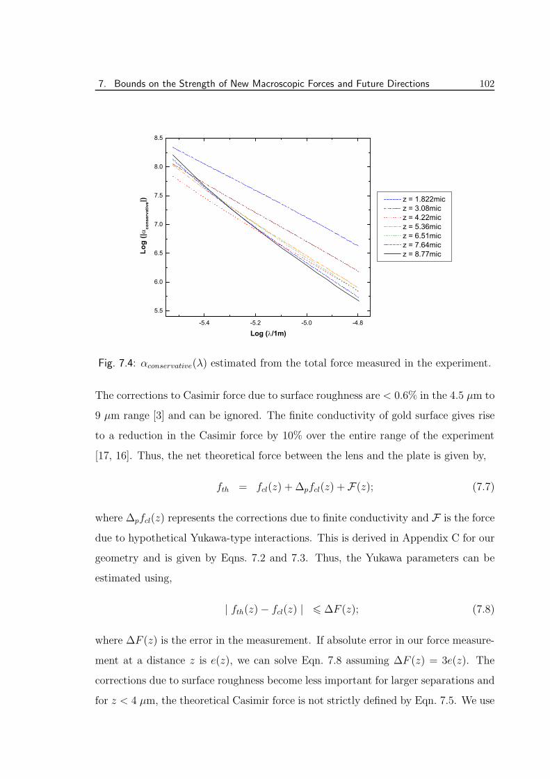
7. Bounds on the Strength of New Macroscopic Forces and Future Directions 102
-5.4 -5.2 -5.0 -4.8
5.5
6.0
6.5
7.0
7.5
8.0
8.5
z = 1.822mic z = 3.08mic z = 4.22mic z = 5.36mic z = 6.51mic z = 7.64mic z = 8.77mic
Log
(|co
nser
vativ
e|)
Log ( /1m)
Fig. 7.4: αconservative(λ) estimated from the total force measured in the experiment.
The corrections to Casimir force due to surface roughness are < 0.6% in the 4.5 µm to
9 µm range [3] and can be ignored. The finite conductivity of gold surface gives rise
to a reduction in the Casimir force by 10% over the entire range of the experiment
[17, 16]. Thus, the net theoretical force between the lens and the plate is given by,
fth = fcl(z) + ∆pfcl(z) + F(z); (7.7)
where ∆pfcl(z) represents the corrections due to finite conductivity and F is the force
due to hypothetical Yukawa-type interactions. This is derived in Appendix C for our
geometry and is given by Eqns. 7.2 and 7.3. Thus, the Yukawa parameters can be
estimated using,
| fth(z)− fcl(z) | 6 ∆F (z); (7.8)
where ∆F (z) is the error in the measurement. If absolute error in our force measure-
ment at a distance z is e(z), we can solve Eqn. 7.8 assuming ∆F (z) = 3e(z). The
corrections due to surface roughness become less important for larger separations and
for z < 4 µm, the theoretical Casimir force is not strictly defined by Eqn. 7.5. We use
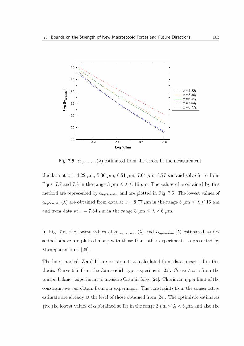
7. Bounds on the Strength of New Macroscopic Forces and Future Directions 103
-5.4 -5.2 -5.0 -4.85.0
5.5
6.0
6.5
7.0
7.5
8.0
z = 4.22 z = 5.36 z = 6.51 z = 7.64 z = 8.77
Log
(|op
timis
tic|)
Log ( /1m)
Fig. 7.5: αoptimistic(λ) estimated from the errors in the measurement.
the data at z = 4.22 µm, 5.36 µm, 6.51 µm, 7.64 µm, 8.77 µm and solve for α from
Eqns. 7.7 and 7.8 in the range 3 µm ≤ λ ≤ 16 µm. The values of α obtained by this
method are represented by αoptimistic and are plotted in Fig. 7.5. The lowest values of
αoptimistic(λ) are obtained from data at z = 8.77 µm in the range 6 µm ≤ λ ≤ 16 µm
and from data at z = 7.64 µm in the range 3 µm ≤ λ < 6 µm.
In Fig. 7.6, the lowest values of αconservative(λ) and αoptimistic(λ) estimated as de-
scribed above are plotted along with those from other experiments as presented by
Mostepanenko in [26].
The lines marked ‘Zerolab’ are constraints as calculated from data presented in this
thesis. Curve 6 is from the Canvendish-type experiment [25]. Curve 7, a is from the
torsion balance experiment to measure Casimir force [24]. This is an upper limit of the
constraint we can obtain from our experiment. The constraints from the conservative
estimate are already at the level of those obtained from [24]. The optimistic estimates
give the lowest values of α obtained so far in the range 3 µm ≤ λ < 6 µm and also the
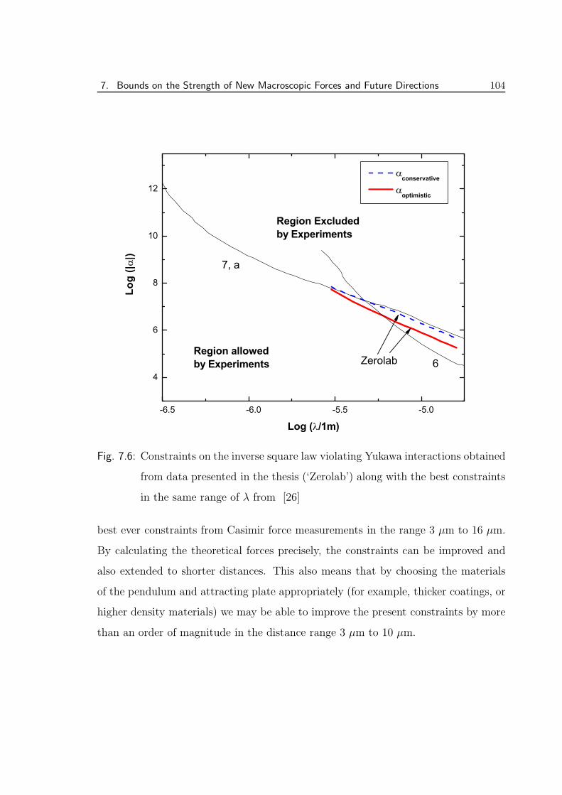
7. Bounds on the Strength of New Macroscopic Forces and Future Directions 104
-6.5 -6.0 -5.5 -5.0
4
6
8
10
12
conservative
optimistic
Lo
g (|
|)
Log ( /1m)
7, a
6Zerolab
Region Excludedby Experiments
Region allowedby Experiments
Fig. 7.6: Constraints on the inverse square law violating Yukawa interactions obtained
from data presented in the thesis (‘Zerolab’) along with the best constraints
in the same range of λ from [26]
best ever constraints from Casimir force measurements in the range 3 µm to 16 µm.
By calculating the theoretical forces precisely, the constraints can be improved and
also extended to shorter distances. This also means that by choosing the materials
of the pendulum and attracting plate appropriately (for example, thicker coatings, or
higher density materials) we may be able to improve the present constraints by more
than an order of magnitude in the distance range 3 µm to 10 µm.
7. Bounds on the Strength of New Macroscopic Forces and Future Directions 105
7.2 Future Directions
We are in the process of performing a next generation experiment, with the same gen-
eral configuration but improved precision by reducing the systematic and statistical
noise. In the new scheme we will perform a null experiment where the deflection of
the pendulum due to the torque from the lens is balanced by the capacitive torques
from a pair of metal plates located close to the disc of the pendulum (see §2.3). Thevoltages on capacitor plates are controlled through a servo-loop and the servo-signal
is a direct measure of the torques acting on the balance. This mode of experiment
has several advantages. The gain in the feed-back helps to reduce the noise in the
system (see for example [18]). The statistical accuracy can be considerably improved
by increasing the integration time. The errors associated with the estimation of ac-
celeration from the limited time series data are avoided. The experiment can be
performed at closer separations as well. The torque due the lens can be modulated
by moving the lens back and forth, further reducing the noise in the bandwidth of the
observation. Efforts are also on to characterize the background electrostatic forces
better and hence decrease systematic errors.
With the lens-plate combination, Casimir force at separations greater than 30 µm
will be difficult to measure as electrostatic and gravitational forces will start to dom-
inate. A similar experiment would be repeated with a flat plate instead of a lens for
separation up to about 100 µm. The parallelism between this plate and suspension
disc is less critical at these separations. The dependance of the Casimir force on
separation will be 1/d3 as opposed to the typical 1/d2 or 1/d dependance of the other
background forces. Such an experiment will be able to put stronger constraints on
the new forces with strength close to that of gravity in the sub-millimeter range as
the parallel plate configuration maximizes the sensitivity to these forces as opposed
to the plate-sphere experiments.
We expect a 5% accurate measurement of the Casimir force in the range 10 µm to
References 106
100 µm, and also improved constraints on hypothetical Yukawa-type forces with range
10 µm to 100 µm, from these future experiments.
References
[1] E. G. Adelberger, B. R. Heckel, and A. E. Nelson. Tests of the Gravitational
Inverse-Square Law. Ann. Rev. of Nuclear and Particle Science, 53:77-121 2003.
[2] N. Arkani-Hamed, S. Dimopoulos, and G. Dvali. Phenomenology, astrophysics,
and cosmology of theories with submillimeter dimensions and TeV scale quantum
gravity. Phys. Rev. D, 59:086004, April 1999.
[3] M. Bordag, B. Geyer, G. L. Klimchitskaya, and V. M. Mostepanenko. Constraints
for hypothetical interactions from a recent demonstration of the Casimir force
and some possible improvements. Phys. Rev. D, 58:075003, October 1998.
[4] M. Bordag, U. Mohideen, and V. M. Mostepanenko. New Developements in
Casimir Force. Phys. Rep., 353:1, 2001.
[5] R Cowsik. A new torsion balance for studies in gravitation and cosmology. Indian
Journal of Physics, 55B:487, 1981.
[6] R Cowsik. Challenges in experimental gravitation and cosmology. Technical
report, Dept. of Science & Technology, New Delhi, 1982.
[7] R Cowsik. Search for new forces in nature. In From Mantle to Meteorites (Prof.
D.Lal Festschrift), 1990.
[8] R. Cowsik, N. Krishnan, P. Sarawat, S. N Tandon, and S. Unnikrishnan. The
Fifth Force Experiment at the TIFR. In Gravitational Measurements, Funda-
mental Metrology and Constants, 1988.
[9] R. Cowsik, N. Krishnan, P. Sarawat, S. N Tandon, and S. Unnikrishnan. Limits
on the strength of the fifth-force. In Advances in Space Research (Proc. XXI
COSPAR, Espoo), 1989.
References 107
[10] R. Cowsik, N. Krishnan, S. N. Tandon, and C. S. Unnikrishnan. Limit on the
strength of intermediate-range forces coupling to isospin. Physical Review Letters,
61:2179–2181, November 1988.
[11] R. Cowsik, S. N Tandon, and N. Krishnan. Sensitive test of Equivalence Princi-
ple. Technical report, Dept. of Science & Technology, New Delhi, 1982.
[12] S. Cullen and M. Perelstein. SN 1987A Constraints on Large Compact Dimen-
sions. Physical Review Letters, 83:268–271, July 1999.
[13] R. S. Decca, E. Fischbach, G. L. Klimchitskaya, D. E. Krause, D. Lopez, and
V. M. Mostepanenko. Improved tests of extra-dimensional physics and thermal
quantum field theory from new Casimir force measurements. Phys. Rev. D,
68:116003, December 2003.
[14] E. Fischbach, D. E. Krause, V. M. Mostepanenko, and M. Novello. New con-
straints on ultrashort-ranged Yukawa interactions from atomic force microscopy.
Phys. Rev. D, 64:075010, October 2001.
[15] E. Fischbach and C. L. Talmadge. The Search for Non-Newtonian Gravity. The
Search for Non-Newtonian Gravity, XVII, 305 pp. 58 figs.. Springer-Verlag New
York, 1999.
[16] C. Genet. La Force de Casimir Entre Deux Miroirs Metalliques A temperature
Non Nulle. PhD thesis, Laboratoire Kastler Brossel, University of Paris, Paris,
Italy, 1999.
[17] C. Genet, A. Lambrecht, and S. Reynaud. Temperature dependence of the
Casimir effect between metallic mirrors. Phy.Rev. A, 62:012110, July 2000.
[18] F. Grassia, J.-M. Courty, S. Reynaud, and P. Touboul. Quantum theory of
fluctuations in a cold damped accelerometer. European Physical Journal D,
8:101–110, 2000.
References 108
[19] J. H. Gundlach, G. L. Smith, E. G. Adelberger, B. R. Heckel, and H. E. Swanson.
Short-Range Test of the Equivalence Principle. Physical Review Letters, 78:2523–
2526, March 1997.
[20] C. Hanhart, D. R. Phillips, S. Reddy, and M. Savage. Extra dimensions,
SN1987a, and nucleon-nucleon scattering data. Nuclear Physics B, 595:335–359,
February 2001.
[21] C. Hanhart, J. A. Pons, D. R. Phillips, and S. Reddy. The likelihood of GODs’
existence: improving the SN 1987a constraint on the size of large compact di-
mensions. Physics Letters B, 509:1–2, June 2001.
[22] C. D. Hoyle, U. Schmidt, B. R. Heckel, E. G. Adelberger, J. H. Gundlach, D. J.
Kapner, and H. E. Swanson. Submillimeter Test of the Gravitational Inverse-
Square Law: A Search for “Large” Extra Dimensions. Physical Review Letters,
86:1418–1421, February 2001.
[23] N. Krishnan. Search for Intermidiate Range forces Weaker than Gravity. PhD
thesis, Tata Institute of Fundamental Research, Mumbai, India, 1989.
[24] S. K. Lamoreaux. Demonstration of the Casimir Force in the 0.6 to 6 µ Range.
Phys. Rev. Lett, 78:5, 1997.
[25] J. C. Long et al. Upper Limit on Submillimeter-range Forces from Extra Space-
time dimensions. Nature, 421:924, 2003.
[26] V. M. Mostepanenko. Constraints on Non-Newtonian Gravity from Recent
Casimir Force Measurements. ArXiv General Relativity and Quantum Cosmology
e-prints, November 2003.
[27] C. S. Unnikrishnan. Torsion Balance Experiments to Search for New Composition
Dependant Forces. PhD thesis, Tata Institute of Fundamental Research, Mumbai,
India, 1992.

APPENDIX
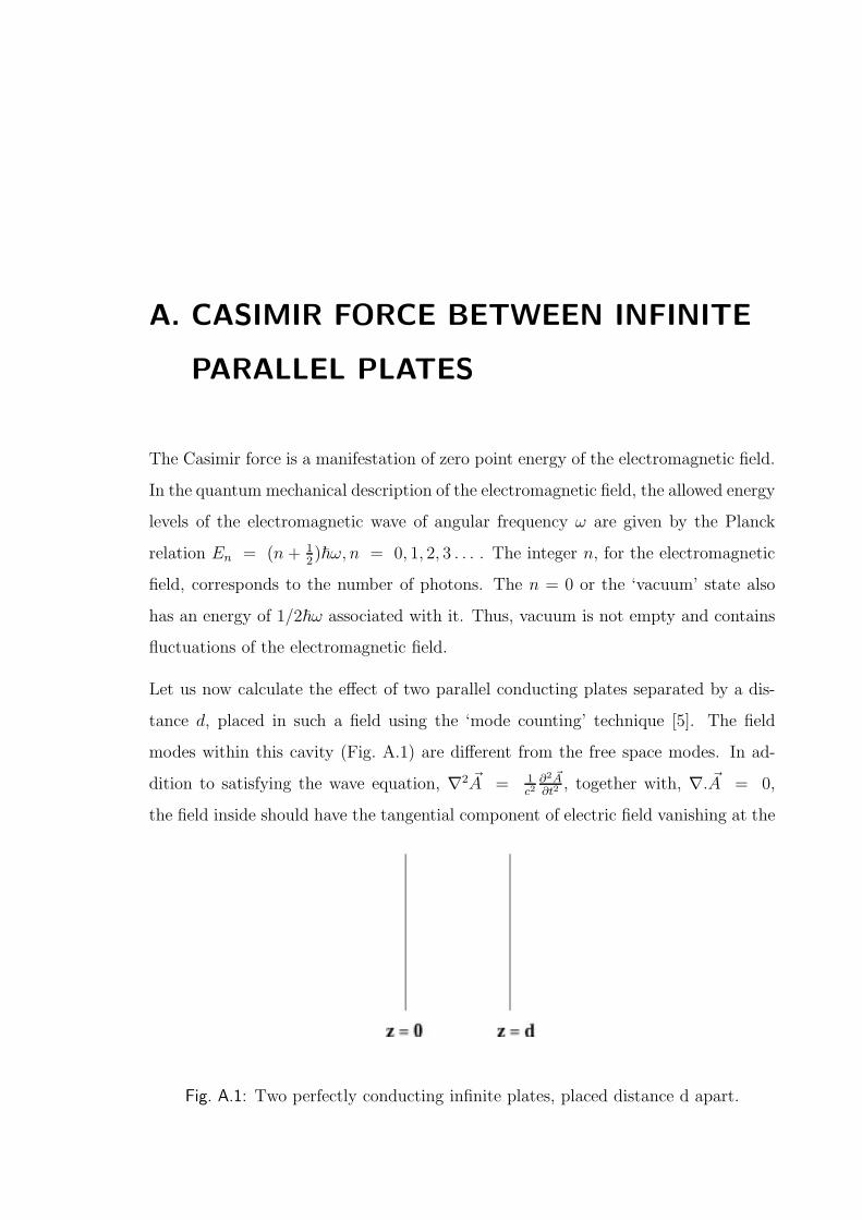
A. CASIMIR FORCE BETWEEN INFINITE
PARALLEL PLATES
The Casimir force is a manifestation of zero point energy of the electromagnetic field.
In the quantum mechanical description of the electromagnetic field, the allowed energy
levels of the electromagnetic wave of angular frequency ω are given by the Planck
relation En = (n + 12)~ω, n = 0, 1, 2, 3 . . . . The integer n, for the electromagnetic
field, corresponds to the number of photons. The n = 0 or the ‘vacuum’ state also
has an energy of 1/2~ω associated with it. Thus, vacuum is not empty and contains
fluctuations of the electromagnetic field.
Let us now calculate the effect of two parallel conducting plates separated by a dis-
tance d, placed in such a field using the ‘mode counting’ technique [5]. The field
modes within this cavity (Fig. A.1) are different from the free space modes. In ad-
dition to satisfying the wave equation, ∇2 ~A = 1c2
∂2 ~A∂t2
, together with, ∇. ~A = 0,
the field inside should have the tangential component of electric field vanishing at the
Fig. A.1: Two perfectly conducting infinite plates, placed distance d apart.
A. Casimir Force between infinite Parallel Plates 111
perfectly conducting boundaries. The solution that satisfies these conditions is given
by,
~A(~r) = Ax(r)x+ Ay(r)y + Az(r)z; (A.1)
where Ax(r) =
√
8
Vax cos kxx sin kyy sin kzz, (A.2)
Ay(r) =
√
8
Vax sin kxx cos kyy sin kzz, (A.3)
Az(r) =
√
8
Vax sin kxx sin kyy cos kzz; (A.4)
with,
a2x + a2y + a2z = 1;V = L2Lz & (A.5)
kx =πl
L; ky =
πm
L; kz =
πn
L; where l, m, n = 0, 1, 2, 3, . . . (A.6)
∇. ~A = 0 also requires that
kxAx + kyAy + kzAz = 0 or (A.7)
π
L(lAx +mAx) +
π
Lz(nAz) = 0. (A.8)
There are two polarizations possible for each value of l, m, n unless one of them is
zero. In that case, only one polarization is possible due to Eqn. A.8. Thus, the
allowed modes within the cavity are,
ωlmn = klmnc = πc
(
l2
L2+
m2
L2+
n2
L2
)1
2
. (A.9)
The zero-point energy of the field inside is,
E(d) =∑
lmn
′ 21
2~ωlmn =
∑
lmn
′ π~c
(
l2
L2+
m2
L2+
n2
L2
)1
2
. (A.10)
The factor 2 arises from the 2 independent polarizations for l, m, n 6= 0 and the prime
on∑
indicates that when l or m or n = 0, a factor of half has to be inserted.
A. Casimir Force between infinite Parallel Plates 112
When L >> Lz = d,∑
lmn
′ −→∑
n
′(
L
π
)2 ∫ ∫
dkxdky and
E(d) =∑
lmn
′ 21
2~ωlmn (A.11)
=
(
L
π
)2
~c
∞∑
n=0
′∫ ∞
0
∫ ∞
0
dkxdky
(
k2x + k2
y +n2π2
d2
)1
2
(A.12)
This is infinite. Outside the cavity,∑
n will also be replaced by dπ
∫
dkz and
E(∞) =
(
L
π
)2
~cd
π
∫ ∞
0
∫ ∞
0
∫ ∞
0
dkxdkydkz(
k2x + k2
y + k2z
)1
2 . (A.13)
This is also infinite. But the potential energy of the system when the plates are
separated by a distance d is U(d) = E(d)− E(∞).
U(d) =
(
L
π
)2
~c
[ ∞∑
n=0
′∫ ∞
0
∫ ∞
0
dkxdky
(
k2x + k2
y +n2π2
d2
)1
2
− d
π
∫ ∞
0
∫ ∞
0
∫ ∞
0
dkxdkydkz(
k2x + k2
y + k2z
)1
2
]
. (A.14)
In polar co-ordinates, u, θ in kx, ky plane, dkxdky = ududθ, θ ranges from 0 to π/2
for positive kx, ky, and we have,
U(d) =
(
L
π
)2
~cπ
2
[
∑
n
′∫ ∞
0
du u
(
u2 +n2π2
d2
)1
2
− d
π
∫ ∞
0
dkz
∫ ∞
0
du u(
u2 + k2z
)1
2
]
(A.15)
This is still infinite. We now introduce a cut-off function f(k) = f([u2 + k2]1/2)
such that f(k) = 1 for k << km and f(k) = 0 for k >> km. We could say that for
wavelengths comparable to atomic dimensions, the assumption of perfect conductivity
breaks down and hence a cut-off is necessary (km ≈ 1/a0, a0 is Bohr radius). Thus,
A. Casimir Force between infinite Parallel Plates 113
Eqn. A.15 becomes,
U(d) =
(
L
π
)2
~cπ
2
∞∑
(n=0)
′∫ ∞
0
du u
(
u2 +n2π2
d2
)1
2
f([u2 + k2]1
2 )
− d
π
∫ ∞
0
dkz
∫ ∞
0
du u(
u2 + k2z
)1
2 f([u2 + k2]1
2 )
]
(A.16)
Defining x ≡ u2d2/π2 & κ = kzd/π, (A.17)
=L2
~c
4π
π3
d3
[
∑
n
′∫ ∞
0
dx(
x+ n2)
1
2 f(π
d[x+ k2]
1
2 )
−∫ ∞
0
dκ
∫ ∞
0
dx(
x+ κ2)
1
2 f(π
d[x+ κ2]
1
2 )
]
. (A.18)
Now,
U(d) =π2~c
4d3
[
1
2F (0) +
∞∑
n=1
F (n)−∫ ∞
0
dκF (κ)
]
; (A.19)
where F (κ) ≡∫ ∞
0
dx(
x+ κ2)
1
2 f(π
d[x+ κ2]
1
2 ). (A.20)
According to Euler-Maclarin summation formula [1],
∞∑
n=1
F (n)−∫ ∞
0
dκF (κ) = −1
2F (0)− 1
12F ′(0) +
1
720F ′′(0) + · · · , (A.21)
for F (∞) → 0. To evaluate F n(0), we note that,
F (κ) =
∫ ∞
κ2
du√uf(
π
d
√u), F ′(κ) = −2κ2f(
π
dκ). (A.22)
Then F ′(0) = 0, F ′′′(0) = −4 and F n(0) = 0 for n > 3, if the cut-off function vanishes
at κ = 0. Thus,
∞∑
n=1
F (n)−∫ ∞
0
dκF (κ) = −1
2F (0)− 4
720(A.23)
U(d) =π2~c
4d3L2
(
− 4
720
)
(A.24)
=π2~c
720d3L2 (A.25)
which is finite and independent of the cut-off function. The attractive force per unit
area,
Fc(d) = − π2~c
240d3, (A.26)
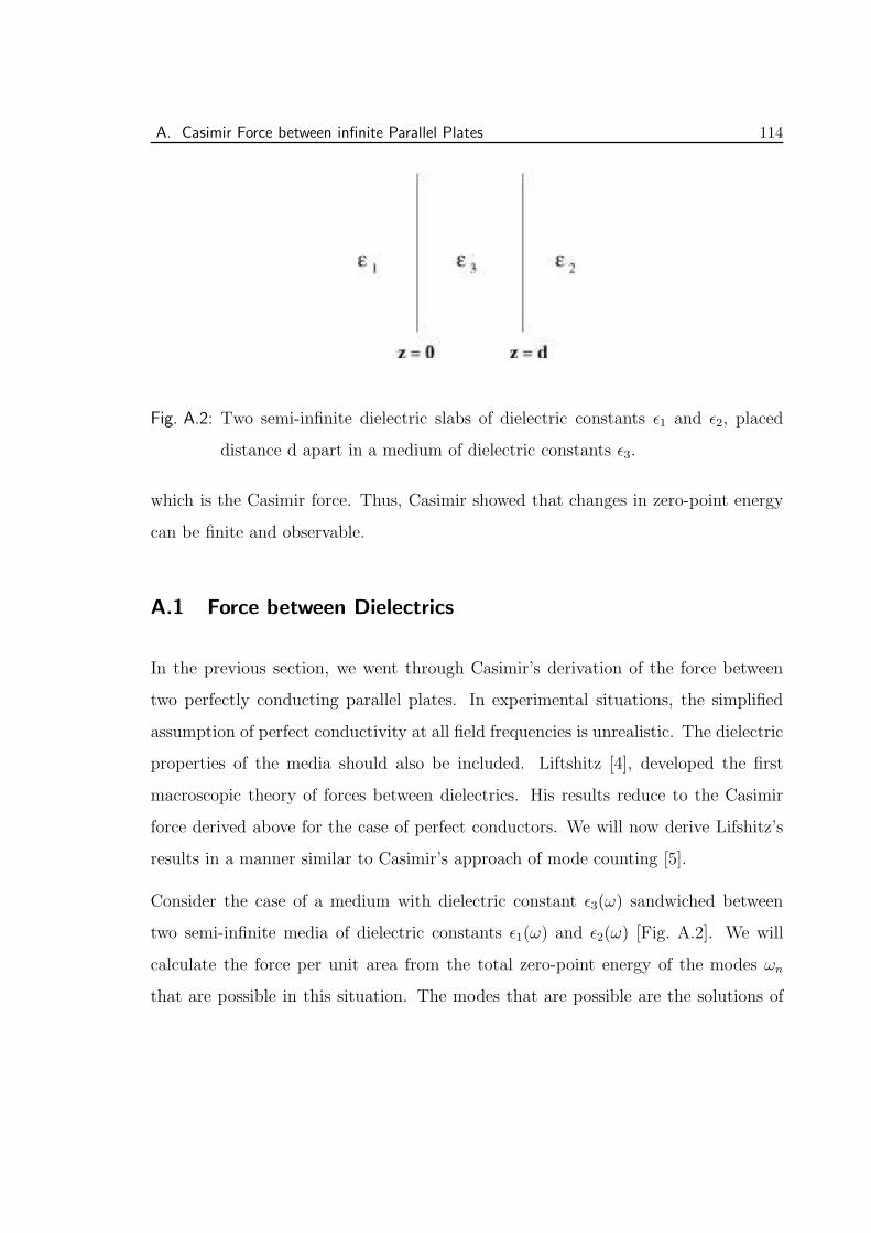
A. Casimir Force between infinite Parallel Plates 114
Fig. A.2: Two semi-infinite dielectric slabs of dielectric constants ǫ1 and ǫ2, placed
distance d apart in a medium of dielectric constants ǫ3.
which is the Casimir force. Thus, Casimir showed that changes in zero-point energy
can be finite and observable.
A.1 Force between Dielectrics
In the previous section, we went through Casimir’s derivation of the force between
two perfectly conducting parallel plates. In experimental situations, the simplified
assumption of perfect conductivity at all field frequencies is unrealistic. The dielectric
properties of the media should also be included. Liftshitz [4], developed the first
macroscopic theory of forces between dielectrics. His results reduce to the Casimir
force derived above for the case of perfect conductors. We will now derive Lifshitz’s
results in a manner similar to Casimir’s approach of mode counting [5].
Consider the case of a medium with dielectric constant ǫ3(ω) sandwiched between
two semi-infinite media of dielectric constants ǫ1(ω) and ǫ2(ω) [Fig. A.2]. We will
calculate the force per unit area from the total zero-point energy of the modes ωn
that are possible in this situation. The modes that are possible are the solutions of
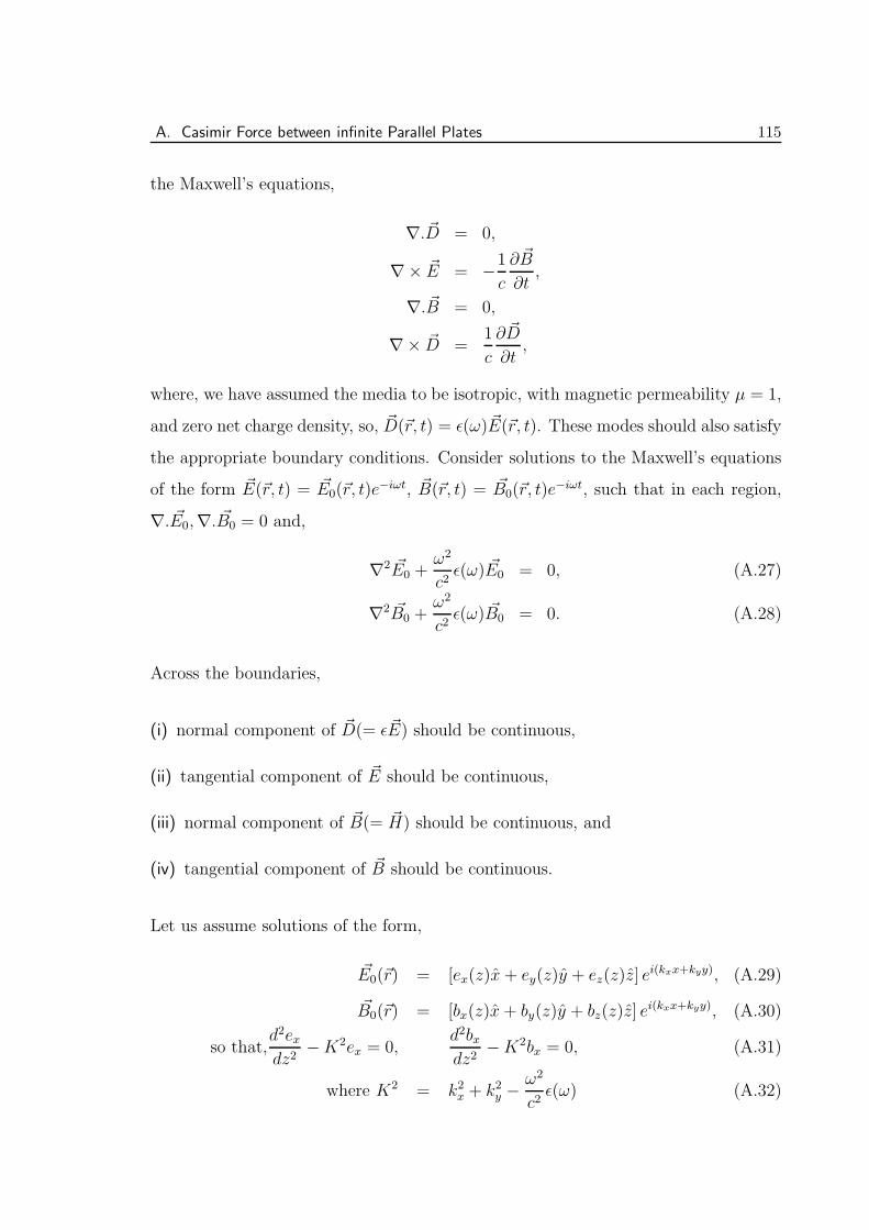
A. Casimir Force between infinite Parallel Plates 115
the Maxwell’s equations,
∇. ~D = 0,
∇× ~E = −1
c
∂ ~B
∂t,
∇. ~B = 0,
∇× ~D =1
c
∂ ~D
∂t,
where, we have assumed the media to be isotropic, with magnetic permeability µ = 1,
and zero net charge density, so, ~D(~r, t) = ǫ(ω) ~E(~r, t). These modes should also satisfy
the appropriate boundary conditions. Consider solutions to the Maxwell’s equations
of the form ~E(~r, t) = ~E0(~r, t)e−iωt, ~B(~r, t) = ~B0(~r, t)e
−iωt, such that in each region,
∇. ~E0,∇. ~B0 = 0 and,
∇2 ~E0 +ω2
c2ǫ(ω) ~E0 = 0, (A.27)
∇2 ~B0 +ω2
c2ǫ(ω) ~B0 = 0. (A.28)
Across the boundaries,
(i) normal component of ~D(= ǫ ~E) should be continuous,
(ii) tangential component of ~E should be continuous,
(iii) normal component of ~B(= ~H) should be continuous, and
(iv) tangential component of ~B should be continuous.
Let us assume solutions of the form,
~E0(~r) = [ex(z)x + ey(z)y + ez(z)z] ei(kxx+kyy), (A.29)
~B0(~r) = [bx(z)x+ by(z)y + bz(z)z] ei(kxx+kyy), (A.30)
so that,d2exdz2
−K2ex = 0,d2bxdz2
−K2bx = 0, (A.31)
where K2 = k2x + k2
y −ω2
c2ǫ(ω) (A.32)
A. Casimir Force between infinite Parallel Plates 116
and likewise for y and z components. In free space, ǫ(ω) = 1 everywhere for all ω and
the usual plane wave solutions are obtained for K2 < 0; k2x+k2
y+k2z =
ω2
c2, K2 = −k2
z .
For the case under consideration, let us assume ǫ(ω) to be real and K2 > 0 in all three
media. We can chose a coordinate system in which ky = 0 and K2 = k2−ǫ(ω)ω2
c2, k ≡
kx.
∇ ~E0 = 0, implies that ikex +dezdz
= 0. (A.33)
∇× ~E0 = iωc~B0, gives
~B0(~r) =
[
ic
ω
deydz
x− c
ω
(
kez + idexdz
)
y +c
ωkey z
]
eikx. (A.34)
∇. ~B0 is also identically satisfied by Eqn. A.34.
The boundary conditions mentioned above imply,
(i) ǫ(ω)ez(z) should be continuous,
(ii) ex should be continuous which is satisfied if dexdz
is continuous (from Eqn. A.33),
and
(iii) ey should be continuous,
(iv) deydz
and kez + idexdz
should be continuous,
But, from Eqn. A.32 and A.33, kez + idexdz
= 1kǫ(ω)ω
2
c2ez. Thus, all conditions are
satisfies if,
a. ǫ(ω)ez(z) anddexdz
are continuous, and
b. ey and deydz
are continuous.
Now, since d2ezdz2
−K2ez = 0, in each region, ignoring exponential growing solutions,
we have,
ez(z) = Aek1z, for z < 0; (A.35)
= Bek3z + Ce−k3z, for 0 ≤ z ≤ 0; (A.36)
= De−k2z, for z > 0; (A.37)
A. Casimir Force between infinite Parallel Plates 117
where K2j ≡ k2 − ǫj(ω)
ω2
c2. Applying the boundary conditions ‘a’, we have,
− ǫ1A+ ǫ3B + ǫ3C = 0; (A.38)
−K1A+K3B −K3C = 0; (A.39)
ǫ3eK3dB + ǫ3e
−K3dC − ǫ2eK2dD = 0; (A.40)
K3eK3dB −K3e
−K3dC +K2eK2dD = 0. (A.41)
For non-trivial solutions to exist,
∣
∣
∣
∣
∣
∣
∣
∣
∣
∣
∣
∣
−ǫ1 ǫ3 ǫ3 0
−K1 K3 −K3 0
0 ǫ3eK3d ǫ3e
−K3d −ǫ2e−K2d
0 K3eK3d −K3e
−K3d K2e−K2d
∣
∣
∣
∣
∣
∣
∣
∣
∣
∣
∣
∣
= 0.
This yields,ǫ3K1 + ǫ1K3
ǫ3K1 − ǫ1K3.ǫ3K2 + ǫ2K3
ǫ3K2 − ǫ1K3.e2K3d − 1 = 0. (A.42)
Similarly, it can be shown that the boundary conditions ‘b’ are satisfied if,
K1 +K3
K1 −K3.K2 +K3
K2 −K3.e2K3d − 1 = 0. (A.43)
Equations A.42 and A.43 are the conditions on the allowed modes ωn. Both cannot
in general be satisfied simultaneously. For boundary conditions a and b to be satis-
fied simultaneously; (a) Eqn. A.42 should be satisfied with ey ≡ 0 or (b) Eqn. A.43
should be satisfied with ez ≡ 0. Thus we have two kinds of modes. Since these are
exponentially decaying functions of z for z < 0 and z > d, these are called surface
modes [2].
Let us now calculate the zero-point energy of these modes. The energy is given by,
E(d) =∑
n
1
2~ωna +
∑
n
1
2~ωnb, (A.44)
A. Casimir Force between infinite Parallel Plates 118
where ωna are the modes of type (a) and ωnb are the modes of type (b). Since kx and
ky are continuous, the summations over them in ωnα, α = a, b can be replaced with
integrals.
∑
x
→(
L
2π
)2 ∫
dkx
∫
dky∑
N
=
(
L
2π
)2 ∫
2πkdk∑
N
, (A.45)
where L is the length along x and y sides of the ‘quantization box’ and∑
N denotes
sum over the solutions of A.42 and A.43. Thus,
E(d) =~L2
4π
∫ ∞
0
dk k
[
∑
N
ωNa(k) +∑
N
ωNb(k)
]
. (A.46)
In order to evaluate this summation, we employ the ‘argument theorem’ from the
theory of functions of complex variables: for a function f(z) which is analytic except
for poles on and inside a simple closed circle C,
1
2πi
∮
C
f ′(z)
f(z)dz = N − P, (A.47)
where N is the number of zeros and P the number of poles f(z) inside C (see for
example, [3]). It can be shown from this that,
1
2πi
∮
C
zf ′(z)
f(z)dz =
[
∑
i
zi
]
f(zi)=0
−[
∑
i
zi
]
f(zi)=∞
; (A.48)
= sum of zero′s of f(zi) inside C (A.49)
− sum of poles of f(zi) inside C. (A.50)
Let Fa(ω) and Fb(ω) be the L.H.S of Eqns. A.42 and A.43 then,
∑
N
ωNα(K) = sum of zero′s of Fα, α = a, b. (A.51)
The poles of Fα, considered as function of complex variable ω, are independent of the
boundaries and hence of d. Therefore,
1
2πi
∮
C
ωF ′α(ω)
Fα(ω)dω =
∑
N
ωNα(K)− (Term independant of d). (A.52)
The ωNα(K) of interest are those that are positive and real. Hence, the closed curve
C is defined by the imaginary axis of complex ω plane and a semicircle in the right
A. Casimir Force between infinite Parallel Plates 119
half of this plane, with radius extending to infinity. As the d dependant term does
not contribute to the force, for this analysis, we can write,
E(d) =~L2
4π
1
2πi
∫ ∞
0
dk k
[∮
C
ωF ′a(ω)
Fa(ω)dω +
∮
C
ωF ′b(ω)
Fb(ω)dω
]
. (A.53)
Each of these contour integrals, can be written as a part along the imaginary axis
and a part along the infinite semicircle. The later integral is d-independent and does
not contribute to the force. The former integral is,
∫ −∞
∞iξ
1
Fα(iξ)
∂Fα(iξ)
∂(iξ)idξ = −i
∫ −∞
∞dξ ξ
G′α(ξ)
Gα(ξ); (A.54)
= −i
∫ −∞
∞dξ ξ
d
dξlogGα(ξ); (A.55)
= i
∫ ∞
−∞dξ logGα(ξ); (A.56)
where Gα(ξ) ≡ Fα(iξ), α = a, b. Writing explicitly,
Ga(ξ) =ǫ3K1 + ǫ1K3
ǫ3K1 − ǫ1K3
.ǫ3K2 + ǫ2K3
ǫ3K2 − ǫ1K3
.e2K3d − 1; (A.57)
Gb(ξ) =K1 +K3
K1 −K3
.K2 +K3
K2 −K3
.e2K3d − 1; (A.58)
where, now ǫj = ǫj(iξ) and K2j = k2 + ǫj(iξ)
ξ2
c2. The zero-point energy associated
with the allowed modes is then,
E(d) =~L2
8π2
∫ ∞
0
dk k
[∫ ∞
−∞dξ logGa(ξ) +
∫ ∞
−∞dξ logGa(ξ)
]
+ d independant term.
(A.59)
The force F (d) = − ∂∂dE(d),
F (d) = −~L2
8π2
∂
∂d
[∫ ∞
0
dk k
{∫ ∞
−∞dξ logGa(ξ) +
∫ ∞
−∞dξ logGb(ξ)
}]
. (A.60)
But, from equation A.57 and A.58, ∂∂dGα(ξ) = 2K3 (Gα + 1), and
∂
∂d
∫ ∞
−∞dξ logGα(ξ) =
∫ ∞
−∞dξ
∂
∂dlogGα(ξ); (A.61)
=
∫ ∞
−∞dξ
1
Gα(ξ)[2K3 (Gα + 1)] ; (A.62)
= 2
∫ ∞
−∞dξ K3 + 2
∫ ∞
−∞dξ
K3
Gα(ξ). (A.63)
A. Casimir Force between infinite Parallel Plates 120
The first term is independent of the presence of the dielectric slabs and hence is not
related to the force between them. Therefore, the force per unit area,
F (d) = − ~
8π2
∫ ∞
0
dk k
∫ ∞
−∞dξ 2K3
[
1
Ga(ξ)+
1
Gb(ξ)
]
. (A.64)
Kj and ǫj are even functions of ξ, and so is Gα; Hence
F (d) = − ~
2π2
∫ ∞
0
dk k
∫ ∞
0
dξ K3
[
1
Ga(ξ)+
1
Gb(ξ)
]
. (A.65)
More explicitly,
F (d) = − ~
2π2
∫ ∞
0
dk k
∫ ∞
0
dξ K3
[
{
ǫ3K1 + ǫ1K3
ǫ3K1 − ǫ1K3
.ǫ3K2 + ǫ2K3
ǫ3K2 − ǫ1K3
.e2K3d − 1
}−1
+
{
K1 +K3
K1 −K3
.K2 +K3
K2 −K3
.e2K3d − 1
}−1]
; (A.66)
where, ǫj = ǫj(iξ) and K2j = k2 + ǫj(iξ)
ξ2
c2.
To compare with Lifshitz theory we introduce a variable p such that,
k2 = ǫ3ξ2
c2(
p2 − 1)
. (A.67)
Then, K23 = k2 + ǫ3
ξ2
c2= ǫ3
ξ2
c2p2; (A.68)
andK21,2 = k2 + ǫ1,2
ξ2
c2= ǫ3
ξ2
c2(
p2 − 1)
+ ǫ1,2ξ2
c2;
= ǫ3ξ2
c2
(
p2 − 1 +ǫ1,2ǫ3
)
;
≡ ǫ3ξ2
c2s21,2, where s21,2 = p2 − 1 +
ǫ1,2ǫ3
. (A.69)
Changing to these set of variables, dk k = ǫ3ξ2
c2dp p and,
F (d) = − ~
2π2c3
∫ ∞
1
dp p2∫ ∞
0
dξ ξ3ǫ3/23
[
{
ǫ3s1 + ǫ1p
ǫ3s1 − ǫ1p.ǫ3s2 + ǫ2p
ǫ3s2 − ǫ1p.e2ξp
√ǫ3d/c − 1
}−1
+
{
s1 + p
s1 − p.s2 + p
s2 − p.e2ξp
√ǫ3d/c − 1
}−1]
(A.70)
A. Casimir Force between infinite Parallel Plates 121
For the case when there is vacuum between the slabs, (ǫ3 = 1),
F (d) = − ~
2π2c3
∫ ∞
1
dp p2∫ ∞
0
dξ ξ3
[
{
s1 + ǫ1p
s1 − ǫ1p.s2 + ǫ2p
s2 − ǫ1p.e2ξpd/c − 1
}−1
+
{
s1 + p
s1 − p.s2 + p
s2 − p.e2ξpd/c − 1
}−1]
. (A.71)
which matches with Lifshitz’s result [4].
A.2 Casimir force at finite temperature
When we derived the Casimir pressure between the dielectric slabs, we assumed the
vacuum state for the field and added only the zero-point energy of the allowed modes
to calculate the energy of the field. At any finite temperature,
En =
(
n(ω) +1
2
)
~ω, where n(ω) =1
e~ω
kBT − 1. (A.72)
Thus to calculate the energy of the allowed modes at a finite temperature, we have
to use Eqn. A.72, rather than just 12~ω,
ET>0(d) = E(d).
(
n(ω) + 12
)
12
; (A.73)
= E(d).2.
(
1
e~ω
kBT − 1+
1
2
)
; (A.74)
= E(d) coth~ω
2kBT. (A.75)
The easiest way to now derive the force expression is to use ω = iξ in Eqn. A.71 and
multiply by the factor coth ~ω2kBT
. For simplicity, let ǫ3 = 1, K3 = −iωcp and,
F (d) = − ~
2π2c3
∫ ∞
1
dp p2∫ ∞
0
dω ω3
[
{
s1 + ǫ1p
s1 − ǫ1p.s2 + ǫ2p
s2 − ǫ1p.e−2iωpd/c − 1
}−1
+
{
s1 + p
s1 − p.s2 + p
s2 − p.e−2iωpd/c − 1
}−1]
coth~ω
2kBT. (A.76)
A. Casimir Force between infinite Parallel Plates 122
To evaluate this integral, we could use ω → iξ as before. But, coth ~ω2kBT
has poles on
the imaginary axis at ωn = 2πinkBT~
≡ iξn, for all integer n. So the closed curve C will
now have semicircles around these poles in the path that runs along imaginary axis.
The integration along the semicircles about ωn contribute iπ times the residue of the
integrand at ωn for n > 0 and at n = 0 it will contribute iπ2from the quarter circle.
F (d) = − ~
2π2c32πikBT
~i3
∞∑
n=0
′ξ3∫ ∞
1
dp p2
[
{
ǫ1np
s1n − ǫ1np.s2n + ǫ2np
s2n − ǫ1np.e2ξnpd/c − 1
}−1
+
{
s1n + p
s1n − p.s2n + p
s2n − p.e2ξnpd/c − 1
}−1]
; (A.77)
where sjn =√
p2 − 1 + ǫjn, ǫjn = ǫj(iξn), j = 1, 2 and the prime on the summation
sign indicates that a factor half must be included in n = 0 term. This result was first
derived by Lifshitz [4]. For the case when ǫ1,2 → ∞,
F (d) = −kBT
πc3
∞∑
n=0
′ξ3∫ ∞
1
dp p2(
2
e2ξnpd/c − 1
)
;
= −2kBT
πc3
∞∑
n=0
′ξ3∫ ∞
1
dpp2
e2ξnpd/c − 1; (A.78)
= −2kBT
πc3c3
8d3
∞∑
n=0
′∫ ∞
nx
dyy2
ey − 1; (A.79)
where x ≡ 4πkBTd~c
. When x ≫ 1, the dominant contribution if from the n = 0 term
F (d) = − kBT
4πd31
2
∫ ∞
0
dyy2
ey − 1; (A.80)
= −ζ(3)kBT
4πd3. (A.81)
Note that the distance dependance changes from 1/d4 at ‘low temperature’ to 1/d3
at ‘high temperature’. Also, the high and low temperature regime are defined by the
dimensionless parameter x ≡ 4πkBTd~c
. At any given temperature T , we can always
choose a large enough d, such that x ≫ 1. Thus, low or high temperature is equivalent
to smaller or larger separations.
References 123
References
[1] M. Abramowitz and Stegun I. A. Handbook of Mathematical Functions. Dover
Books, Newyork, 1971.
[2] G. Barton. Some Surface Effects in the Hydrodynamic Model of Metals. Rep.
Prog. Phys., 42:963, 1979.
[3] M. L Boas. Mathematical Methods in the Physical Sciences. Wiley, Newyork,
1983.
[4] E. M. Lifshitz. Theory of molecular attraction between solids. Sov. Phys. JETP,
2:73, 1956.
[5] W. P Milonni. The Quantum Vacuum: An Introduction to Quantum Electrody-
namics. Academic Press, Newyork, 1994.
B. CASIMIR FORCE BETWEEN
SPHERICAL LENS AND FLAT PLATE
The Casimir force per unit area between two parallel conducting plates, at T = 0 K
is given by,
fc0(z) = − π2~c
240z4(B.1)
= −0.013
z4µdyn.cm−2 where zµ ≡ z in microns. (B.2)
For a finite temperature T we approximate the distance dependence as
fcT (z) = fc0(z), for z < λT ; (B.3)
fcT (z) = fc0(z)z
λT, for z > λT . (B.4)
For convenience, we write Eqns. B.1 and B.4 as,
fc0(z) ≡ −Ac
z4dyn.cm−2, (B.5)
fcT (z) ≡ − Ac
λT z3dyn.cm−2, (B.6)
where Ac =π2~c
240. (B.7)
The Casimir force between the lens and plate can now be estimated using the “Der-
jaguin (proximity) approximation”, often called “proximity theorem” [1]. Here the
total force is calculated by integrating over concentric rings on the lens surface that
are equidistant from the plate. Thus, the Casimir force between the lens and plate is
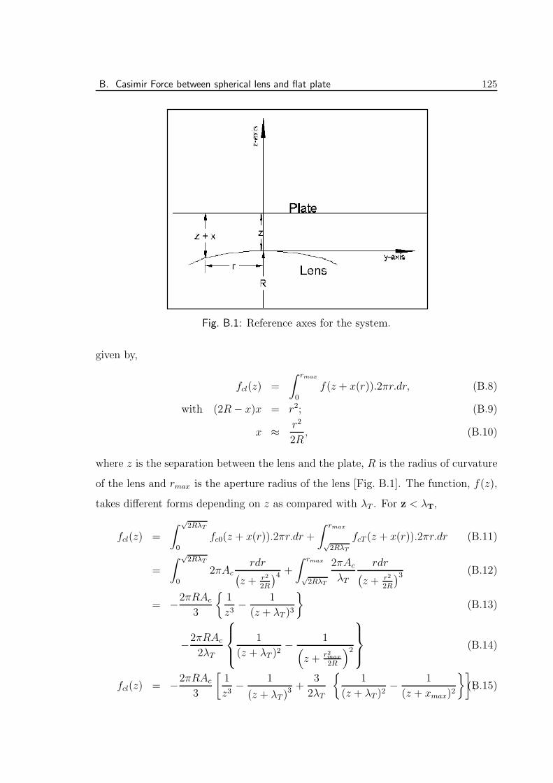
B. Casimir Force between spherical lens and flat plate 125
Fig. B.1: Reference axes for the system.
given by,
fcl(z) =
∫ rmax
0
f(z + x(r)).2πr.dr, (B.8)
with (2R− x)x = r2; (B.9)
x ≈ r2
2R, (B.10)
where z is the separation between the lens and the plate, R is the radius of curvature
of the lens and rmax is the aperture radius of the lens [Fig. B.1]. The function, f(z),
takes different forms depending on z as compared with λT . For z < λT,
fcl(z) =
∫
√2RλT
0
fc0(z + x(r)).2πr.dr +
∫ rmax
√2RλT
fcT (z + x(r)).2πr.dr (B.11)
=
∫
√2RλT
0
2πAcrdr
(
z + r2
2R
)4 +
∫ rmax
√2RλT
2πAc
λT
rdr(
z + r2
2R
)3 (B.12)
= −2πRAc
3
{
1
z3− 1
(z + λT )3
}
(B.13)
−2πRAc
2λT
1
(z + λT )2− 1(
z + r2max
2R
)2
(B.14)
fcl(z) = −2πRAc
3
[
1
z3− 1
(z + λT )3 +
3
2λT
{
1
(z + λT )2− 1
(z + xmax)2
}]
;(B.15)
References 126
where xmax = r2max
2R. For z > λT,
fcl(z) =
∫ rmax
0
fcT (z + x(r)).2πr.dr (B.16)
= −πRAc
λT
[
1
z2− 1
(z + xmax)2
]
. (B.17)
References
[1] J. Blocki et al. . Ann. Phys. (N.Y.), 105:427, 1977.
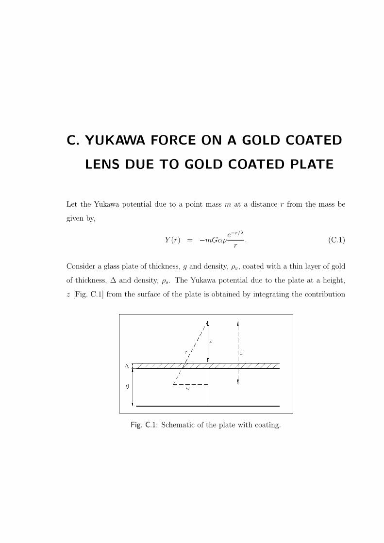
C. YUKAWA FORCE ON A GOLD COATED
LENS DUE TO GOLD COATED PLATE
Let the Yukawa potential due to a point mass m at a distance r from the mass be
given by,
Y (r) = −mGαρe−r/λ
r. (C.1)
Consider a glass plate of thickness, g and density, ρv, coated with a thin layer of gold
of thickness, ∆ and density, ρs. The Yukawa potential due to the plate at a height,
z [Fig. C.1] from the surface of the plate is obtained by integrating the contribution
Fig. C.1: Schematic of the plate with coating.
C. Yukawa Force on a Gold Coated Lens due to Gold Coated Plate 128
due to various mass elements on the plate,
U(z) = −Gα
∫
ρ(r)e−r/λ
rdV ; (C.2)
where r2 = w2 + z′2. (C.3)
U(z) = −Gα
∫
ρ(z′)e−
√(w2+z′2)/λ
√
(w2 + z′2)2πw dw dz′ (C.4)
= −Gα2π
∫ z
z+g+∆
dz′ ρ(z′)
∫ ∞
z′dr e−r/λ (C.5)
= −2πGαλ
∫ z
z+g+∆
dz′ρ(z′)e−z′/λ (C.6)
= −2πGαλ
(
ρv
∫ z+∆
z+g+∆
dz′ e−z′/λ + ρs
∫ z
z+∆
dz′ e−z′/λ
)
(C.7)
= 2πGαλ2[
ρv{
e−(z+∆)/λ − e−(z+g+∆)/λ}
+
ρs{
e−z/λ − e−(z+∆)/λ}]
. (C.8)
For λ << g, (C.9)
U(z) ≈ 2πGαλ2[
ρve−(z+∆)/λ + ρs
{
e−z/λ − e−(z+∆)/λ}]
. (C.10)
Keeping in mind that our interest is in the region λ << g we use Eqn. C.10 in further
analysis. The force due to this potential is,
f(z) = −∂U
∂z(C.11)
= 2πGαλ[
ρve−(z+∆)/λ + ρs
{
e−z/λ − e−(z+∆)/λ}]
(C.12)
= 2πGαλ[
ρs − (ρs − ρv)e−∆/λ
]
e−z/λ (C.13)
= fce−z/λ; (C.14)
where fc = 2πGαλ[
ρs − (ρs − ρv)e−∆/λ
]
. (C.15)
The lens has a radius of curvature R, a volume density ρl and a surface coating of
uniform thickness δ with density ρc. We now proceed to derive the force on the lens
in two limiting cases: (a) λ << δ and (b) λ >> δ.
Case (a): λ << δ Here the lens may be assumed to be completely made of the coating
material alone.
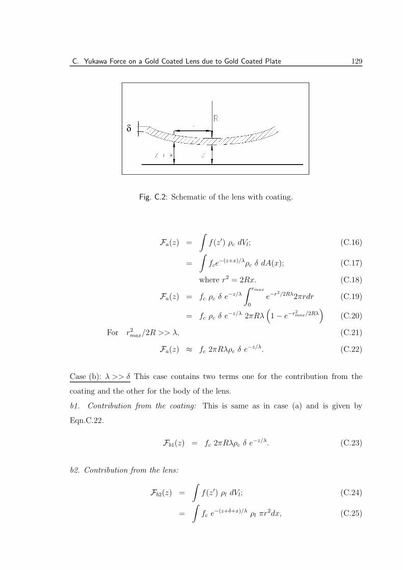
C. Yukawa Force on a Gold Coated Lens due to Gold Coated Plate 129
Fig. C.2: Schematic of the lens with coating.
Fa(z) =
∫
f(z′) ρc dVl; (C.16)
=
∫
fce−(z+x)/λρc δ dA(x); (C.17)
where r2 = 2Rx. (C.18)
Fa(z) = fc ρc δ e−z/λ
∫ rmax
0
e−r2/2Rλ2πrdr (C.19)
= fc ρc δ e−z/λ 2πRλ(
1− e−r2max/2Rλ)
(C.20)
For r2max/2R >> λ, (C.21)
Fa(z) ≈ fc 2πRλρc δ e−z/λ. (C.22)
Case (b): λ >> δ This case contains two terms one for the contribution from the
coating and the other for the body of the lens.
b1. Contribution from the coating: This is same as in case (a) and is given by
Eqn.C.22.
Fb1(z) = fc 2πRλρc δ e−z/λ. (C.23)
b2. Contribution from the lens:
Fb2(z) =
∫
f(z′) ρl dVl; (C.24)
=
∫
fc e−(z+δ+x)/λ ρl πr
2dx, (C.25)
C. Yukawa Force on a Gold Coated Lens due to Gold Coated Plate 130
= fc e−(z+δ)/λ ρl
∫ r2max/2R
0
e−x/λ 2πRxdx (C.26)
= fc e−(z+δ)/λ ρl 2πRλ[
−r2max
2Rer
2max/2Rλ + λ
(
1− er2max/2Rλ
)
]
. (C.27)
For r2max/2R >> λ, (C.28)
Fb2(z) ≈ fc e−(z+δ)/λ ρl 2πRλ. (C.29)
The net force due to Yukawa potential between the lens and the plate for λ >> δ is
given by,
Fb = Fb1 + Fb2 (C.30)
= fc 2πRλ(
ρc δ + ρl λ e−δ/λ)
e−z/λ. (C.31)
In the case our experimental set up, the lens and the plate are both made of the same
material (BK7 glass) and coated with the gold of equal thickness (1 µm). Hence,
ρl = ρv ; ρc = ρs and ∆ = δ (C.32)
Thus, the force in the two cases is given by,
Fa(z) = 4π2GαRλ2[
ρs − (ρs − ρv)e−δ/λ
]
ρs δ e−z/λ, for λ << δ. (C.33)
Fb(z) = 4π2GαRλ2[
ρs − (ρs − ρv)e−δ/λ
] (
ρs δ + ρv λ e−δ/λ)
e−z/λ, (C.34)
for λ >> δ.