A. Hvatov

Torque VibrationIsolatiormasters projectpart I

2015

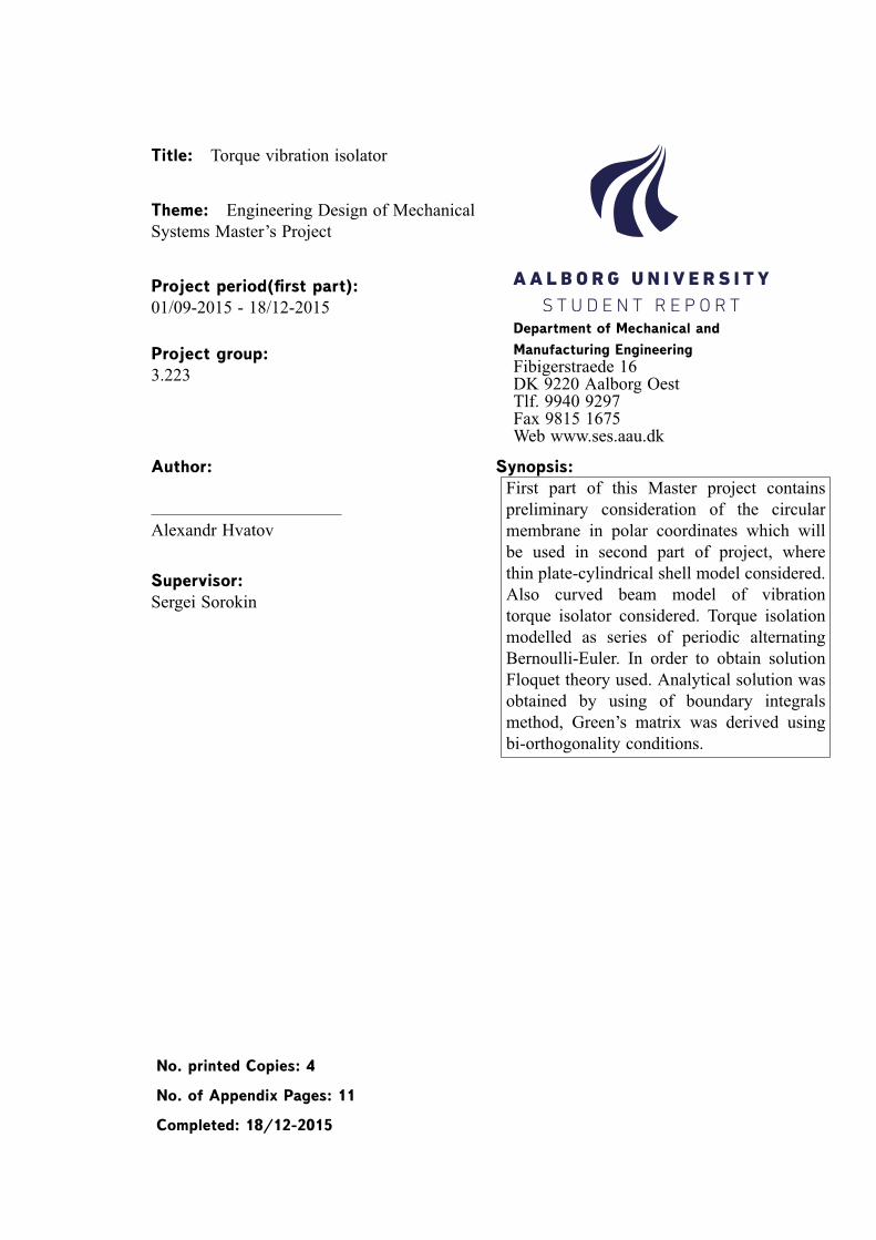
Title: Torque vibration isolator

Theme: Engineering Design of MechanicalSystems Master’s Project

Project period(first part):

01/09-2015 - 18/12-2015

Project group:

3.223

Department of Mechanical and

Manufacturing Engineering

Fibigerstraede 16DK 9220 Aalborg OestTlf. 9940 9297Fax 9815 1675Web www.ses.aau.dk

Author:

Alexandr Hvatov

Supervisor:

Sergei Sorokin

No. printed Copies: 4

No. of Appendix Pages: 11

Completed: 18/12-2015

Synopsis:

First part of this Master project containspreliminary consideration of the circularmembrane in polar coordinates which willbe used in second part of project, wherethin plate-cylindrical shell model considered.Also curved beam model of vibrationtorque isolator considered. Torque isolationmodelled as series of periodic alternatingBernoulli-Euler. In order to obtain solutionFloquet theory used. Analytical solution wasobtained by using of boundary integralsmethod, Green’s matrix was derived usingbi-orthogonality conditions.

Table of contents

Introduction . . . . . . . . . . . . . . . . . . . . . . . . . . . . . . . . . . . . . . . . . . . 5

1 Ch.1. The concept of a periodic structures . . . . . . . . . . . . . . . . . . . . . . . . 7

2 Ch.2 Circular membrane . . . . . . . . . . . . . . . . . . . . . . . . . . . . . . . . . . 92.1 Membrane vibration equation. Green’s function. . . . . . . . . . . . . . . . . . . . 92.2 Periodic structure . . . . . . . . . . . . . . . . . . . . . . . . . . . . . . . . . . . . 13

2.2.1 Infinite structure . . . . . . . . . . . . . . . . . . . . . . . . . . . . . . . . 132.2.2 Finite structures . . . . . . . . . . . . . . . . . . . . . . . . . . . . . . . . . 18

3 Ch.3. Bernoulli-Euler curved beam model . . . . . . . . . . . . . . . . . . . . . . . . 213.1 Equations of motion . . . . . . . . . . . . . . . . . . . . . . . . . . . . . . . . . . . 22

3.1.1 In-plane vibrations . . . . . . . . . . . . . . . . . . . . . . . . . . . . . . . 223.1.2 Out-plane vibrations . . . . . . . . . . . . . . . . . . . . . . . . . . . . . . 25

3.2 Boundary integrals method . . . . . . . . . . . . . . . . . . . . . . . . . . . . . . . 263.2.1 In-plane vibrations . . . . . . . . . . . . . . . . . . . . . . . . . . . . . . . 273.2.2 Out-plane vibrations . . . . . . . . . . . . . . . . . . . . . . . . . . . . . . 28

3.3 The benchmark periodic structure . . . . . . . . . . . . . . . . . . . . . . . . . . . 293.3.1 Infinite periodic structure . . . . . . . . . . . . . . . . . . . . . . . . . . . . 293.3.2 Finite periodic structure . . . . . . . . . . . . . . . . . . . . . . . . . . . . 333.3.3 Eigenmodes analysis . . . . . . . . . . . . . . . . . . . . . . . . . . . . . . 35

3.4 The spatial periodic structure . . . . . . . . . . . . . . . . . . . . . . . . . . . . . . 363.5 Parametric study . . . . . . . . . . . . . . . . . . . . . . . . . . . . . . . . . . . . 37

Conclusion . . . . . . . . . . . . . . . . . . . . . . . . . . . . . . . . . . . . . . . . . . . . 40

Literature . . . . . . . . . . . . . . . . . . . . . . . . . . . . . . . . . . . . . . . . . . . . . 41

A App. А. Circular membrane equation . . . . . . . . . . . . . . . . . . . . . . . . . . . 43

B App. B. Membrane displacement . . . . . . . . . . . . . . . . . . . . . . . . . . . . . . 45

C App. С. Axial rod vibrations . . . . . . . . . . . . . . . . . . . . . . . . . . . . . . . . 47C.1 Green’s function definition and derivation . . . . . . . . . . . . . . . . . . . . . . . 47C.2 Equation of axial displacement of a rod. Boundary integrals method . . . . . . . . . 48C.3 Boundary integrals method direct application . . . . . . . . . . . . . . . . . . . . . 50

D App. D. Floquet theory . . . . . . . . . . . . . . . . . . . . . . . . . . . . . . . . . . . 53

3

Introduction

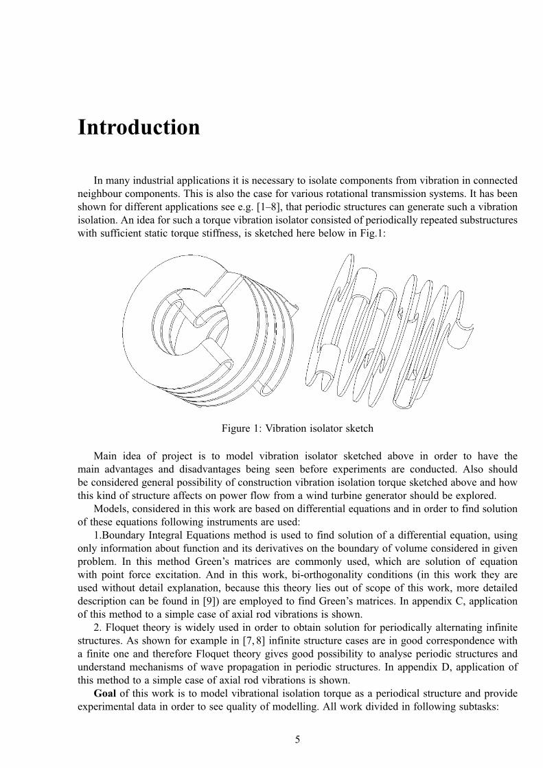
In many industrial applications it is necessary to isolate components from vibration in connectedneighbour components. This is also the case for various rotational transmission systems. It has beenshown for different applications see e.g. [1–8], that periodic structures can generate such a vibrationisolation. An idea for such a torque vibration isolator consisted of periodically repeated substructureswith sufficient static torque stiffness, is sketched here below in Fig.1:

Figure 1: Vibration isolator sketch

Main idea of project is to model vibration isolator sketched above in order to have themain advantages and disadvantages being seen before experiments are conducted. Also shouldbe considered general possibility of construction vibration isolation torque sketched above and howthis kind of structure affects on power flow from a wind turbine generator should be explored.

Models, considered in this work are based on differential equations and in order to find solutionof these equations following instruments are used:

1.Boundary Integral Equations method is used to find solution of a differential equation, usingonly information about function and its derivatives on the boundary of volume considered in givenproblem. In this method Green’s matrices are commonly used, which are solution of equationwith point force excitation. And in this work, bi-orthogonality conditions (in this work they areused without detail explanation, because this theory lies out of scope of this work, more detaileddescription can be found in [9]) are employed to find Green’s matrices. In appendix C, applicationof this method to a simple case of axial rod vibrations is shown.

2. Floquet theory is widely used in order to obtain solution for periodically alternating infinitestructures. As shown for example in [7, 8] infinite structure cases are in good correspondence witha finite one and therefore Floquet theory gives good possibility to analyse periodic structures andunderstand mechanisms of wave propagation in periodic structures. In appendix D, application ofthis method to a simple case of axial rod vibrations is shown.

Goal of this work is to model vibrational isolation torque as a periodical structure and provideexperimental data in order to see quality of modelling. All work divided in following subtasks:

5

(I) Show possibility of using Floquet theory in polar coordinates on example of circularmembrane equation, since isolator, shown on a Fig.1 contains part, that is modelled as a part ofthe circular plate, which equation is naturally written in polar coordinate system. Floquet theory iswell studied in cartesian coordinate system [1], but there are no works, where application of Floquettheory to other coordinate systems is shown.

(II) Derivation and evaluation of boundary integral equations for a beam model (first model),based on Bernoulli-Euler flat ring equations

(III) Derivation and evaluation of boundary integral equations for a Kirchoff-Love plate andcylindricall shell model (second model) with use of polar coordinates

(IV) Experimental validation of first and second modelSince it is a long master’s project in first part only subtasks (I) (Ch.2) and (II) (Ch.3) are

considered. Parts (III) and (IV) will be covered in second part of project.Project is written in comprehensive way and information in appendix can be used as supply for

more clear understanding of methods, that lies in ground of this project. Information in appendicesis not mandatory for understanding ideas of this project.

6

Chapter 1

The concept of a periodic structures

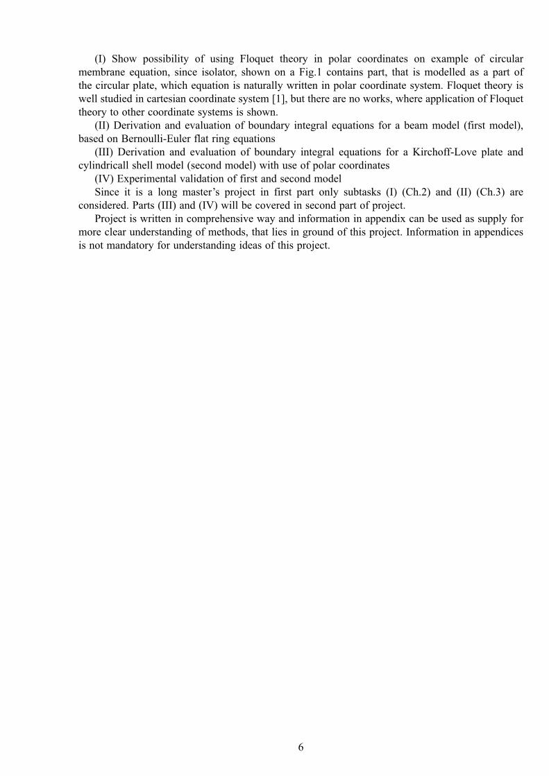
Here common definitions for all periodic structures considered in this work are introduced. First,an infinite periodic structure as shown on Fig.1.1 can be considered:

Figure 1.1: Infinite periodical structure scheme

,where 𝜉 is the common coordinate (axial coordinate of bar, radial coordinate of a circularmembrane, natural coordinate of spring). Each component of a periodic structure can have differentmaterial parameters (like Young modulus), shape parameters (like curvature) and length repeating inperiodic alternating manner. In order to use Floquet theory at least one parameter excluding lengthshould be different for two segments. In terms of vibrations, different wavenumbers 𝑘𝑖 for each partare required.

The existence of frequency stop- and pass-bands in infinite periodic waveguides is well knownand understood since the pioneering work by L.Brillouin [1]. The vibro-acoustics of beams, platesand shells and pipes with periodic attachments or step-wise varying properties has been broadlyexplored by many authors. Classial works [1, 2] and the modern one [3–8] are just a few of those,which illustrate the classical and recent advances in this area of research and that it is of interestto develop methods for various waveguides and make industrial application of theory of periodicstructures.

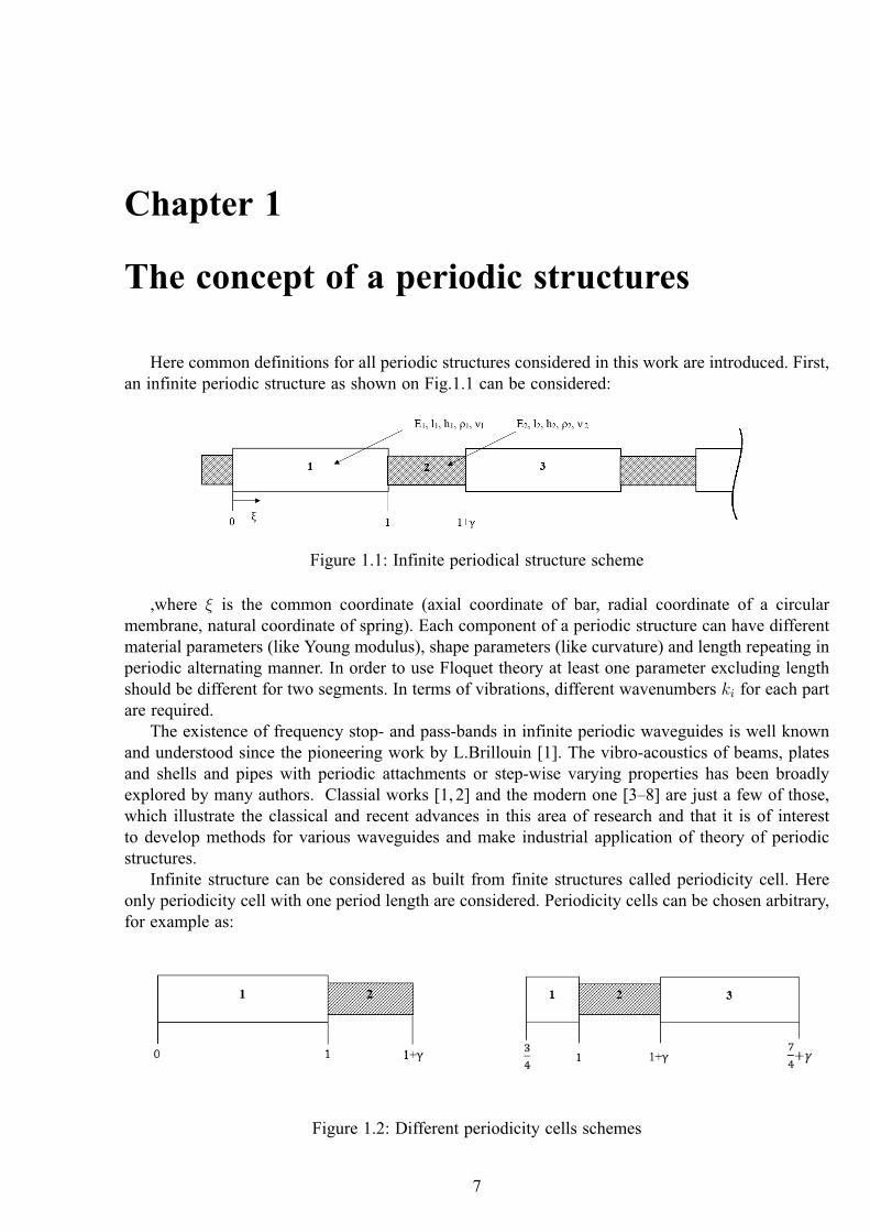
Infinite structure can be considered as built from finite structures called periodicity cell. Hereonly periodicity cell with one period length are considered. Periodicity cells can be chosen arbitrary,for example as:

Figure 1.2: Different periodicity cells schemes

7

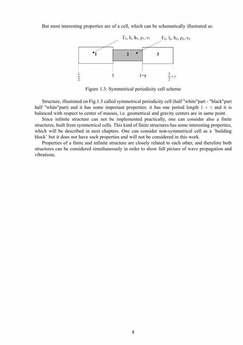
But most interesting properties are of a cell, which can be schematically illustrated as:

Figure 1.3: Symmetrical periodicity cell scheme

Structure, illustrated on Fig.1.3 called symmetrical periodicity cell (half "white"part - "black"parthalf "white"part) and it has some important properties: it has one period length 1 + 𝛾 and it isbalanced with respect to center of masses, i.e. geometrical and gravity centers are in same point.

Since infinite structure can not be implemented practically, one can consider also a finitestructures, built from symmetrical cells. This kind of finite structures has some interesting properties,which will be described in next chapters. One can consider non-symmetrical cell as a ’buildingblock’ but it does not have such properties and will not be considered in this work.

Properties of a finite and infinite structure are closely related to each other, and therefore bothstructures can be considered simultaneously in order to show full picture of wave propagation andvibrations.

8

Chapter 2

Periodic circular membrane

Torque vibration isolator shown on Fig.1 can be considered as an ensemble of flat ring plates andcylindrical shells, connected in an alternative manner, i.e. as a periodic structure. Equation of motionof flat ring plate is naturally written in the polar coordinate system. Therefore, it is expedient toinvestigate performance of a periodic structure in polar coordinates. Previously in [7] and [8] mostsimple cases of axial and flexural vibrations of periodic beams and vibrations of cylindrical shellwere considered. Main ideas of these articles were shown for cartesian coordinate system. Maingoal of this chapter is to consider different coordinate system and show that all properties of theperiodic structures for cartesian coordinates are preserved in polar coordinate system with simplecircular membrane as an illustrative example.

2.1 Membrane vibration equation. Green’s function.

General equation of motion for the membrane has the form (see App.A for derivation fromHamilton’s principle and [10]):(

∆ + 𝑘2)𝑢 = 𝑢𝑟𝑟 +

1

𝑟𝑢𝑟 +

1

𝑟2𝑢𝜙𝜙 + 𝑘2𝑢 = −𝑞(𝑟, 𝜙) (2.1)

,where 𝑞(𝑟, 𝜙) is the intensity of distributed force.The external force can be presented as:

𝑞 (𝑟, 𝜙) =+∞∑𝑚=0

𝑄𝑚(𝑟) cos(𝑚𝜙) (2.2)

Then general solution can also be expanded in Fourier series :

𝑢 (𝑟, 𝜙) =+∞∑𝑚=0

𝑈𝑚(𝑟) cos(𝑚𝜙) (2.3)

Which substituted into Eq.2.1 gives:

(∆ + 𝑘2

)𝑢 =

+∞∑𝑚=0

(𝜕2𝑈𝑚(𝑟)

𝜕𝑟2+

1

𝑟

𝜕𝑈𝑚(𝑟)

𝜕𝑟+ (𝑘2 − 𝑚2

𝑟2)𝑈𝑚(𝑟)

)cos(𝑚𝜙) = −

+∞∑𝑚=0

𝑄𝑚(𝑟) cos(𝑚𝜙)

(2.4)Since cos𝑚𝜑 are independent functions, for each circumferential wave number 𝑚 decoupled

equation can be solved (hereafter, index 𝑚 is omitted in all equations):

𝑈 ′′(𝑟) +1

𝑟𝑈 ′(𝑟) +

(𝑘2 − 𝑚2

𝑟2

)𝑈(𝑟) = −𝑄(𝑟) (2.5)

9

In order to obtain solution Green’s function method is used. By definition [11], Green’s functionis a solution of the equation ( in what follows 𝜕

𝜕𝑟𝐺(𝑟, 𝑟0) = 𝐺′(𝑟, 𝑟0)):

𝐺′′(𝑟, 𝑟0) +1

𝑟𝐺′(𝑟, 𝑟0) +

(𝑘2 − 𝑚2

𝑟2

)𝐺(𝑟, 𝑟0) = −𝛿(𝑟 − 𝑟0) (2.6)

,where 𝛿(𝑥)- Dirac delta function. Here delta function 𝛿(𝑟−𝑟0) has meaning of intensity of pointforce, applied at the point 𝑟0 and distributed in the angular coordinate direction as cos(𝑚𝜙), and 𝑟is the observation point. Therefore second derivative 𝐺′′(𝑟, 𝑟0) has dimension of force intensity

Green’s function of an ordinary second-order differential equation has a following properties [11](for clarity notation of point of excitation and observation preserved).

Symmetry with respect to observation and excitation point property:

𝐺(𝑟, 𝑟0) = 𝐺(𝑟0, 𝑟) (2.7a)

Unit jump in derivative at the excitation point:

𝜕

𝜕𝑟𝐺(𝑟0, 𝑟0 + 𝜀) − 𝜕

𝜕𝑟𝐺(𝑟0, 𝑟0 − 𝜀) = 1, 𝜀 → 0 (2.7b)

Continuity at the excitation point:

𝐺(𝑟0, 𝑟0 + 𝜀) = 𝐺(𝑟0, 𝑟0 − 𝜀), 𝜀 → 0 (2.7c)

It should be noted that ,since second derivative 𝐺′′(𝑟, 𝑟0) has dimension of force intensity,𝜕𝜕𝑟𝐺(𝑟, 𝑟0) in this case has dimension of the force, acting on a radial direction. Therefore, force

should have unit jump at the coordinate 𝑟 = 𝑟0. Also, property of unit jump is a reflection ofmathematical theorem 𝑑

𝑑𝑥𝜃(𝑥) = 𝛿(𝑥), where 𝜃(𝑥) is the Heaviside theta-function. As known, theta-

function has unit jump at the point 𝑥 = 0.Last two properties Eq.2.7b-Eq.2.7c can be used for obtaining explicit form of Green’s function

of equation Eq.2.5. The general solution of equation Eq.2.6 with arbitrary excitation point 𝑟0 has aform:

𝑢+(𝑟) = 𝐴 𝐻(1)𝑚 (𝑘𝑟) , 𝑟 > 𝑟0

𝑢−(𝑟) = 𝐵 𝐻(2)𝑚 (𝑘𝑟) , 𝑟 ≤ 𝑟0

(2.7)

, where 𝐻(1)𝑚 (𝑟) and 𝐻

(2)𝑚 (𝑟) are Hankel’s functions of order 𝑚 of first and second kind

respectively and 𝐴,𝐵 are integration constants.In order to consider infinite structures function 𝑢+(𝑟) should satisfy radiation, or Sommerfeld,

condition [12].With properties Eq.2.7a-Eq.2.7c one can obtain system of linear algebraical equations with

respect to constants 𝐴,𝐵:

𝑢+(𝑟0) = 𝑢−(𝑟0)𝑑𝑑𝑟𝑢+(𝑟0) − 𝑑

𝑑𝑟𝑢−(𝑟0) = 1

(2.8)

Constants are found as:

𝐴 = − 𝐻(2)𝑚 (𝑘 𝑟0)

𝑘(𝐻(1)𝑚+1(𝑘 𝑟0)𝐻

(2)𝑚 (𝑘 𝑟0)−𝐻

(2)𝑚+1(𝑘 𝑟0)𝐻

(1)𝑚 (𝑘 𝑟0))

= −14𝑖𝜋𝑟0𝐻

(2)𝑚 (𝑘 𝑟0)

𝐵 = − 𝐻(1)𝑚 (𝑘 𝑟0)

𝑘(𝐻(1)𝑚+1(𝑘 𝑟0)𝐻

(2)𝑚 (𝑘 𝑟0)−𝐻

(2)𝑚+1(𝑘 𝑟0)𝐻

(1)𝑚 (𝑘 𝑟0))

= −14𝑖𝜋𝑟0𝐻

(1)𝑚 (𝑘 𝑟0)

(2.9)

Thus, Green’s function for equation 2.5 have form:

10

𝐺(𝑟, 𝑟0) =

−1

4𝑖𝜋𝑟0𝐻

(1)𝑚 (𝑘 𝑟0)𝐻

(2)𝑚 (𝑘 𝑟) 𝑟 ≤ 𝑟0

−14𝑖𝜋𝑟0𝐻

(2)𝑚 (𝑘 𝑟0)𝐻

(1)𝑚 (𝑘 𝑟) 𝑟 > 𝑟0

(2.10)

It should be noted, that this form of Green’s function in not unique. One can choose an arbitrarycombination of Bessel functions 𝑌 (𝑟) and 𝐽(𝑟) as the general solution Eq.2.7. Also, any solutionof the homogenous equation Eq.2.5 (with 𝑄(𝑟) ≡ 0) can be added to the existing form of a Green’sfunction.

It is convenient to define Green’s function as a solution of the equation (for more detailedexplanation see App.B):

𝐺′′(𝑟, 𝑟0) +1

𝑟𝐺′(𝑟, 𝑟0) +

(𝑘2 − 𝑚2

𝑟2

)𝐺(𝑟, 𝑟0) = −𝛿(𝑟 − 𝑟0)

𝑟0(2.6’)

From physical point of view, with this definition force resultant 𝐹 =2𝜋∫0

𝑏∫𝑎

− 𝛿(𝑟−𝑟0)𝑟0

𝑟𝑑𝑟𝑑𝜑 =

−2𝜋𝑟0

𝑏∫𝑎

𝛿(𝑟 − 𝑟0)𝑟𝑑𝑟 = −2𝜋𝑟0𝑟0

= −2𝜋 remains constant when point of excitation 𝑟0 is changing.

With definition 2.6’ Green’s function has form:

𝐺(𝑟, 𝑟0) =

−1

2𝑖𝜋𝐻

(1)𝑚 (𝑘 𝑟0)𝐻

(2)𝑚 (𝑘 𝑟) 𝑟 ≤ 𝑟0

−12𝑖𝜋𝐻

(2)𝑚 (𝑘 𝑟0)𝐻

(1)𝑚 (𝑘 𝑟) 𝑟 > 𝑟0

(2.11)

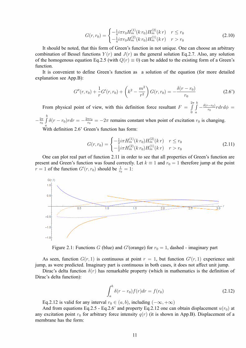
One can plot real part of function 2.11 in order to see that all properties of Green’s function arepresent and Green’s function was found correctly. Let 𝑘 ≡ 1 and 𝑟0 = 1 therefore jump at the point𝑟 = 1 of the function 𝐺′(𝑟, 𝑟0) should be 1

𝑟0= 1:

Figure 2.1: Functions 𝐺 (blue) and 𝐺′(orange) for 𝑟0 = 1, dashed - imaginary part

As seen, function 𝐺(𝑟, 1) is continuous at point 𝑟 = 1, but function 𝐺′(𝑟, 1) experience unitjump, as were predicted. Imaginary part is continuous in both cases, it does not affect unit jump.

Dirac’s delta function 𝛿(𝑟) has remarkable property (which in mathematics is the definition ofDirac’s delta function): ∫ 𝑏

𝑎

𝛿(𝑟 − 𝑟0)𝑓(𝑟)𝑑𝑟 = 𝑓(𝑟0) (2.12)

Eq.2.12 is valid for any interval 𝑟0 ∈ (𝑎, 𝑏), including (−∞,+∞)And from equations Eq.2.5 - Eq.2.6’ and property Eq.2.12 one can obtain displacement 𝑢(𝑟0) at

any excitation point 𝑟0 for arbitrary force intensity 𝑞(𝑟) (it is shown in App.B). Displacement of amembrane has the form:

11

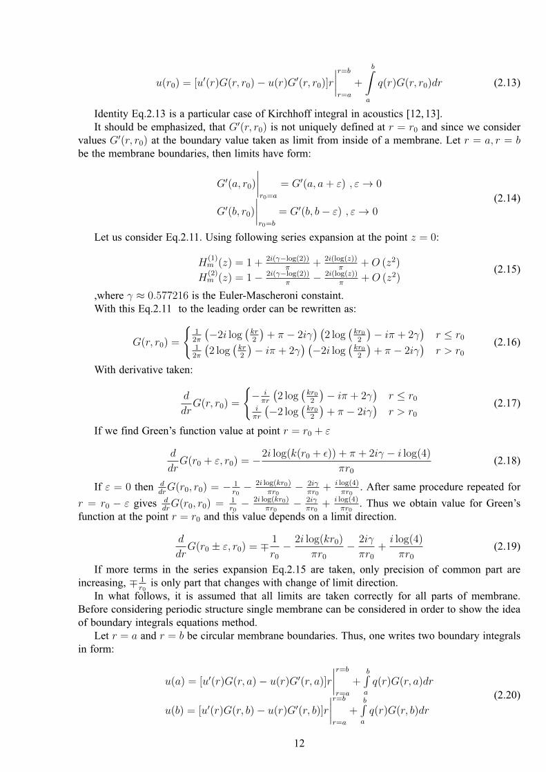
𝑢(𝑟0) = [𝑢′(𝑟)𝐺(𝑟, 𝑟0) − 𝑢(𝑟)𝐺′(𝑟, 𝑟0)]𝑟

𝑟=𝑏

𝑟=𝑎

+

𝑏∫𝑎

𝑞(𝑟)𝐺(𝑟, 𝑟0)𝑑𝑟 (2.13)

Identity Eq.2.13 is a particular case of Kirchhoff integral in acoustics [12, 13].It should be emphasized, that 𝐺′(𝑟, 𝑟0) is not uniquely defined at 𝑟 = 𝑟0 and since we consider

values 𝐺′(𝑟, 𝑟0) at the boundary value taken as limit from inside of a membrane. Let 𝑟 = 𝑎, 𝑟 = 𝑏be the membrane boundaries, then limits have form:

𝐺′(𝑎, 𝑟0)

𝑟0=𝑎

= 𝐺′(𝑎, 𝑎 + 𝜀) , 𝜀 → 0

𝐺′(𝑏, 𝑟0)

𝑟0=𝑏

= 𝐺′(𝑏, 𝑏− 𝜀) , 𝜀 → 0(2.14)

Let us consider Eq.2.11. Using following series expansion at the point 𝑧 = 0:

𝐻(1)𝑚 (𝑧) = 1 + 2𝑖(𝛾−log(2))

𝜋+ 2𝑖(log(𝑧))

𝜋+ 𝑂 (𝑧2)

𝐻(2)𝑚 (𝑧) = 1 − 2𝑖(𝛾−log(2))

𝜋− 2𝑖(log(𝑧))

𝜋+ 𝑂 (𝑧2)

(2.15)

,where 𝛾 ≈ 0.577216 is the Euler-Mascheroni constaint.With this Eq.2.11 to the leading order can be rewritten as:

𝐺(𝑟, 𝑟0) =

12𝜋

(−2𝑖 log

(𝑘𝑟2

)+ 𝜋 − 2𝑖𝛾

) (2 log

(𝑘𝑟02

)− 𝑖𝜋 + 2𝛾

)𝑟 ≤ 𝑟0

12𝜋

(2 log

(𝑘𝑟2

)− 𝑖𝜋 + 2𝛾

) (−2𝑖 log

(𝑘𝑟02

)+ 𝜋 − 2𝑖𝛾

)𝑟 > 𝑟0

(2.16)

With derivative taken:

𝑑

𝑑𝑟𝐺(𝑟, 𝑟0) =

− 𝑖

𝜋𝑟

(2 log

(𝑘𝑟02

)− 𝑖𝜋 + 2𝛾

)𝑟 ≤ 𝑟0

𝑖𝜋𝑟

(−2 log

(𝑘𝑟02

)+ 𝜋 − 2𝑖𝛾

)𝑟 > 𝑟0

(2.17)

If we find Green’s function value at point 𝑟 = 𝑟0 + 𝜀

𝑑

𝑑𝑟𝐺(𝑟0 + 𝜀, 𝑟0) = −2𝑖 log(𝑘(𝑟0 + 𝜖)) + 𝜋 + 2𝑖𝛾 − 𝑖 log(4)

𝜋𝑟0(2.18)

If 𝜀 = 0 then 𝑑𝑑𝑟𝐺(𝑟0, 𝑟0) = − 1

𝑟0− 2𝑖 log(𝑘𝑟0)

𝜋𝑟0− 2𝑖𝛾

𝜋𝑟0+ 𝑖 log(4)

𝜋𝑟0. After same procedure repeated for

𝑟 = 𝑟0 − 𝜀 gives 𝑑𝑑𝑟𝐺(𝑟0, 𝑟0) = 1

𝑟0− 2𝑖 log(𝑘𝑟0)

𝜋𝑟0− 2𝑖𝛾

𝜋𝑟0+ 𝑖 log(4)

𝜋𝑟0. Thus we obtain value for Green’s

function at the point 𝑟 = 𝑟0 and this value depends on a limit direction.

𝑑

𝑑𝑟𝐺(𝑟0 ± 𝜀, 𝑟0) = ∓ 1

𝑟0− 2𝑖 log(𝑘𝑟0)

𝜋𝑟0− 2𝑖𝛾

𝜋𝑟0+

𝑖 log(4)

𝜋𝑟0(2.19)

If more terms in the series expansion Eq.2.15 are taken, only precision of common part areincreasing, ∓ 1

𝑟0is only part that changes with change of limit direction.

In what follows, it is assumed that all limits are taken correctly for all parts of membrane.Before considering periodic structure single membrane can be considered in order to show the ideaof boundary integrals equations method.

Let 𝑟 = 𝑎 and 𝑟 = 𝑏 be circular membrane boundaries. Thus, one writes two boundary integralsin form:

𝑢(𝑎) = [𝑢′(𝑟)𝐺(𝑟, 𝑎) − 𝑢(𝑟)𝐺′(𝑟, 𝑎)]𝑟

𝑟=𝑏

𝑟=𝑎

+𝑏∫𝑎

𝑞(𝑟)𝐺(𝑟, 𝑎)𝑑𝑟

𝑢(𝑏) = [𝑢′(𝑟)𝐺(𝑟, 𝑏) − 𝑢(𝑟)𝐺′(𝑟, 𝑏)]𝑟

𝑟=𝑏

𝑟=𝑎

+𝑏∫𝑎

𝑞(𝑟)𝐺(𝑟, 𝑏)𝑑𝑟

(2.20)

12

Unknown here are two displacements at the boundaries 𝑢(𝑎), 𝑢(𝑏) and two forces 𝑢′(𝑎), 𝑢′(𝑏).In order to close system of algebraic equations two more equations should be written. For singlemembrane these are boundary conditions in form:

𝑢(𝑎) = 0𝑢(𝑏) = 0

(2.21)

or

𝑢′(𝑎) = 0𝑢′(𝑏) = 0

(2.22)

Mixed conditions can be stated too. Main principle is that energy functional should beminimized (see. App.A). In this work only symmetrical boundary conditions are considered.

Eq.2.20,Eq.2.21 or Eq.2.20, Eq.2.22 are four algebraical equations with respect to four unknowns𝑢(𝑎), 𝑢(𝑏), 𝑢′(𝑎), 𝑢′(𝑏) and this system has unique solution. When unknowns are found andsubstituted into Eq.2.13, displacement at any point inside the domain 𝑎 < 𝑟0 < 𝑏 can be found.

2.2 Periodic structure

2.2.1 Infinite structure

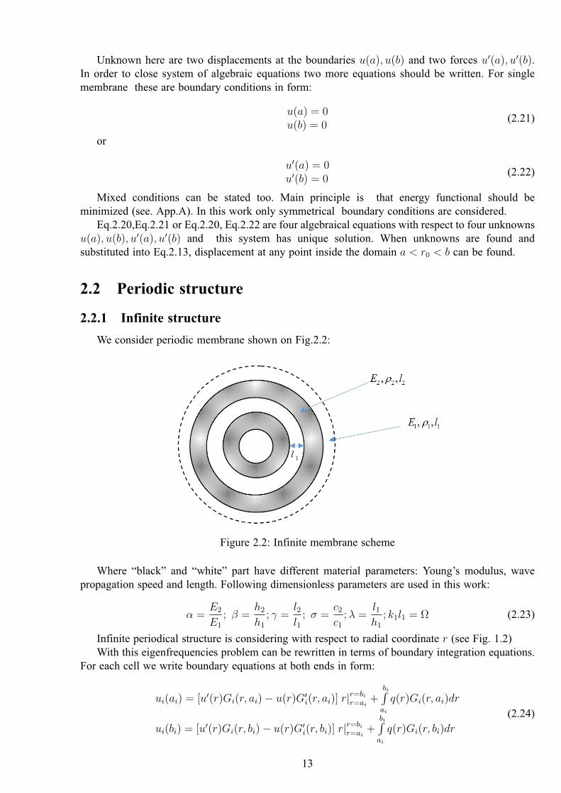
We consider periodic membrane shown on Fig.2.2:

Figure 2.2: Infinite membrane scheme

Where “black” and “white” part have different material parameters: Young’s modulus, wavepropagation speed and length. Following dimensionless parameters are used in this work:

𝛼 =𝐸2

𝐸1

; 𝛽 =ℎ2

ℎ1

; 𝛾 =𝑙2𝑙1

; 𝜎 =𝑐2𝑐1

;𝜆 =𝑙1ℎ1

; 𝑘1𝑙1 = Ω (2.23)

Infinite periodical structure is considering with respect to radial coordinate 𝑟 (see Fig. 1.2)With this eigenfrequencies problem can be rewritten in terms of boundary integration equations.

For each cell we write boundary equations at both ends in form:

𝑢𝑖(𝑎𝑖) = [𝑢′(𝑟)𝐺𝑖(𝑟, 𝑎𝑖) − 𝑢(𝑟)𝐺′𝑖(𝑟, 𝑎𝑖)] 𝑟|

𝑟=𝑏𝑖𝑟=𝑎𝑖

+𝑏𝑖∫𝑎𝑖

𝑞(𝑟)𝐺𝑖(𝑟, 𝑎𝑖)𝑑𝑟

𝑢𝑖(𝑏𝑖) = [𝑢′(𝑟)𝐺𝑖(𝑟, 𝑏𝑖) − 𝑢(𝑟)𝐺′𝑖(𝑟, 𝑏𝑖)] 𝑟|

𝑟=𝑏𝑖𝑟=𝑎𝑖

+𝑏𝑖∫𝑎𝑖

𝑞(𝑟)𝐺𝑖(𝑟, 𝑏𝑖)𝑑𝑟

(2.24)

13

, where 𝑢𝑖 are displacement, 𝑎𝑖 are left and 𝑏𝑖 are right boundaries of 𝑖-th part of membranerespectively. For each part we have 2 unknown displacements and 2 unknown forces at theboundaries.

In order to show main principle one periodicity cell can be considered. Since Bessel 𝑌 (𝑟)function contains singularity at point 𝑟 = 0 the central cell, that contains point 𝑟 = 0 should beexcluded from consideration. Thus, boundary conditions have form:

𝑢2(𝑎2) = [𝑢′(𝑟)𝐺2(𝑟, 𝑎2) − 𝑢(𝑟)𝐺′2(𝑟, 𝑎2)] 𝑟|

𝑟=𝑏2𝑟=𝑎2

+𝑏2∫𝑎2

𝑞(𝑟)𝐺2(𝑟, 𝑎2)𝑑𝑟

𝑢2(𝑏2) = [𝑢′(𝑟)𝐺2(𝑟, 𝑏2) − 𝑢(𝑟)𝐺′2(𝑟, 𝑏2)] 𝑟|

𝑟=𝑏2𝑟=𝑎2

+𝑏2∫𝑎2

𝑞(𝑟)𝐺2(𝑟, 𝑏2)𝑑𝑟

𝑢3(𝑎3) = [𝑢′(𝑟)𝐺3(𝑟, 𝑎3) − 𝑢(𝑟)𝐺′3(𝑟, 𝑎3)] 𝑟|

𝑟=𝑏3𝑟=𝑎3

+𝑏3∫𝑎3

𝑞(𝑟)𝐺3(𝑟, 𝑎3)𝑑𝑟

𝑢3(𝑏3) = [𝑢′(𝑟)𝐺3(𝑟, 𝑏3) − 𝑢(𝑟)𝐺′3(𝑟, 𝑏3)] 𝑟|

𝑟=𝑏3𝑟=𝑎3

+𝑏3∫𝑎3

𝑞(𝑟)𝐺3(𝑟, 𝑏3)𝑑𝑟

(2.25)

As seen, there are four unknown displacements 𝑢2(𝑎2), 𝑢2(𝑏2), 𝑢3(𝑎3), 𝑢3(𝑏3) and four unknownforces 𝑢′

2(𝑎2), 𝑢′2(𝑏2), 𝑢

′3(𝑎3), 𝑢

′3(𝑏3). Therefore four more equations should be added. Two equations

are interfacial conditions between two cells, that allows to consider cells in the system and representscontinuity and forces equilibrium at the interface:

𝑢2(𝑏2) = 𝑢3(𝑎3)𝛼𝑢′

2(𝑏2) = 𝑢′3(𝑎3)

(2.26)

And two last equations are taken from Floquet periodicity theorem. That theorem allows to closesystem in case of infinite structure. Any two points for Floquet conditions can be taken, but withone period distance (1 + 𝛾)𝜆 between points, i.e. 𝑏3 − 𝑎2 = (1 + 𝛾)𝜆:

𝑢2(𝑎2) = Λ𝑢3(𝑏3)𝑢′2(𝑎2) = Λ𝑢′

3(𝑏3)(2.27)

It should be emphasized that if one can consider first cell it is usually written as 𝑢1(𝑏1) insteadof 𝑢2(𝑎2) and 𝑢′

1(𝑏1) instead of 𝑢′2(𝑎2). Nevertheless, that is the same point and therefore it does

not affect the solution.Equations Eq.2.25-Eq.2.27 represent system of eight linear algebraical equations. In load-free

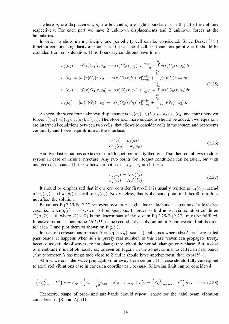
case, i.e. when 𝑞(𝑟) = 0 system is homogeneous. In order to find non-trivial solution condition𝐷(Λ,Ω) = 0, where 𝐷(Λ,Ω) is the determinant of the system Eq.2.25-Eq.2.27, must be fulfilled.In case of circular membrane 𝐷(Λ,Ω) is the second order polynomial in Λ and we can find its rootsfor each Ω and plot them as shown on Fig.2.3.

In case of cartesian coordinates Λ = exp(𝑖𝐾𝐵) (see [1]) and zones where abs(Λ) = 1 are calledpass bands. It happens when 𝐾𝐵 is purely real number. In this case waves can propagate freely,because magnitude of waves are not change throughout the period, changes only phase. But in caseof membrane it is not obviously so, as seen on Fig.2.3 in the zones, similar to cartesian pass bands, the parameter Λ has magnitude close to 2 and it should have another form, than exp(𝑖𝐾𝐵).

At first we consider wave propagation far away from center . This case should fully correspondto axial rod vibrations case in cartesian coordinates , because following limit can be considered:

(∆

(2)𝑝𝑜𝑙𝑎𝑟 + 𝑘2

)𝑢 = 𝑢𝑟𝑟 +

1

𝑟𝑢𝑟 +

1

𝑟2𝑢𝜙𝜙 + 𝑘2𝑢 → 𝑢𝑟𝑟 + 𝑘2𝑢 =

(∆

(1)𝑐𝑎𝑟𝑡𝑒𝑠𝑖𝑎𝑛 + 𝑘2

)𝑢 , 𝑟 → ∞ (2.28)

Therefore, shape of pass- and gap-bands should repeat shape for the axial beam vibrationconsidered in [8] and App.D.

14

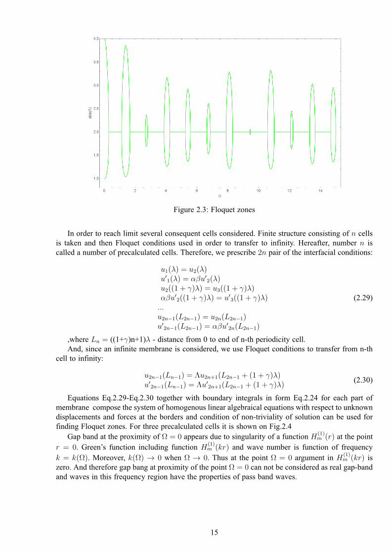
Figure 2.3: Floquet zones

In order to reach limit several consequent cells considered. Finite structure consisting of 𝑛 cellsis taken and then Floquet conditions used in order to transfer to infinity. Hereafter, number 𝑛 iscalled a number of precalculated cells. Therefore, we prescribe 2𝑛 pair of the interfacial conditions:

𝑢1(𝜆) = 𝑢2(𝜆)𝑢′

1(𝜆) = 𝛼𝛽𝑢′2(𝜆)

𝑢2((1 + 𝛾)𝜆) = 𝑢3((1 + 𝛾)𝜆)𝛼𝛽𝑢′

2((1 + 𝛾)𝜆) = 𝑢′3((1 + 𝛾)𝜆)

...𝑢2𝑛−1(𝐿2𝑛−1) = 𝑢2𝑛(𝐿2𝑛−1)𝑢′

2𝑛−1(𝐿2𝑛−1) = 𝛼𝛽𝑢′2𝑛(𝐿2𝑛−1)

(2.29)

,where 𝐿𝑛 = ((1+𝛾)n+1)𝜆 - distance from 0 to end of n-th periodicity cell.And, since an infinite membrane is considered, we use Floquet conditions to transfer from n-th

cell to infinity:

𝑢2𝑛−1(𝐿𝑛−1) = Λ𝑢2𝑛+1(𝐿2𝑛−1 + (1 + 𝛾)𝜆)𝑢′

2𝑛−1(𝐿𝑛−1) = Λ𝑢′2𝑛+1(𝐿2𝑛−1 + (1 + 𝛾)𝜆)

(2.30)

Equations Eq.2.29-Eq.2.30 together with boundary integrals in form Eq.2.24 for each part ofmembrane compose the system of homogenous linear algebraical equations with respect to unknowndisplacements and forces at the borders and condition of non-triviality of solution can be used forfinding Floquet zones. For three precalculated cells it is shown on Fig.2.4

Gap band at the proximity of Ω = 0 appears due to singularity of a function 𝐻(1)𝑚 (𝑟) at the point

𝑟 = 0. Green’s function including function 𝐻(1)𝑚 (𝑘𝑟) and wave number is function of frequency

𝑘 = 𝑘(Ω). Moreover, 𝑘(Ω) → 0 when Ω → 0. Thus at the point Ω = 0 argument in 𝐻(1)𝑚 (𝑘𝑟) is

zero. And therefore gap bang at proximity of the point Ω = 0 can not be considered as real gap-bandand waves in this frequency region have the properties of pass band waves.

15

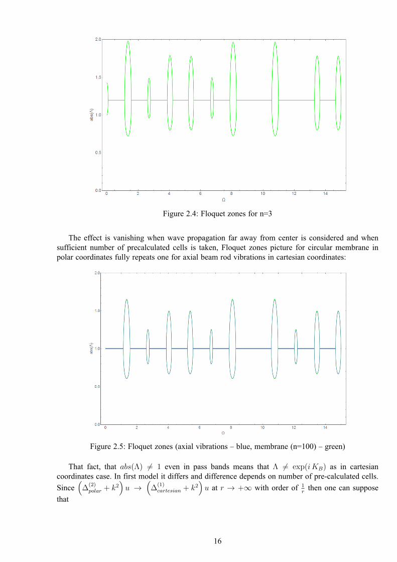
Figure 2.4: Floquet zones for n=3

The effect is vanishing when wave propagation far away from center is considered and whensufficient number of precalculated cells is taken, Floquet zones picture for circular membrane inpolar coordinates fully repeats one for axial beam rod vibrations in cartesian coordinates:

Figure 2.5: Floquet zones (axial vibrations – blue, membrane (n=100) – green)

That fact, that 𝑎𝑏𝑠(Λ) = 1 even in pass bands means that Λ = exp(𝑖𝐾𝐵) as in cartesiancoordinates case. In first model it differs and difference depends on number of pre-calculated cells.

Since(

∆(2)𝑝𝑜𝑙𝑎𝑟 + 𝑘2

)𝑢 →

(∆

(1)𝑐𝑎𝑟𝑡𝑒𝑠𝑖𝑎𝑛 + 𝑘2

)𝑢 at 𝑟 → +∞ with order of 1

𝑟then one can suppose

that

16

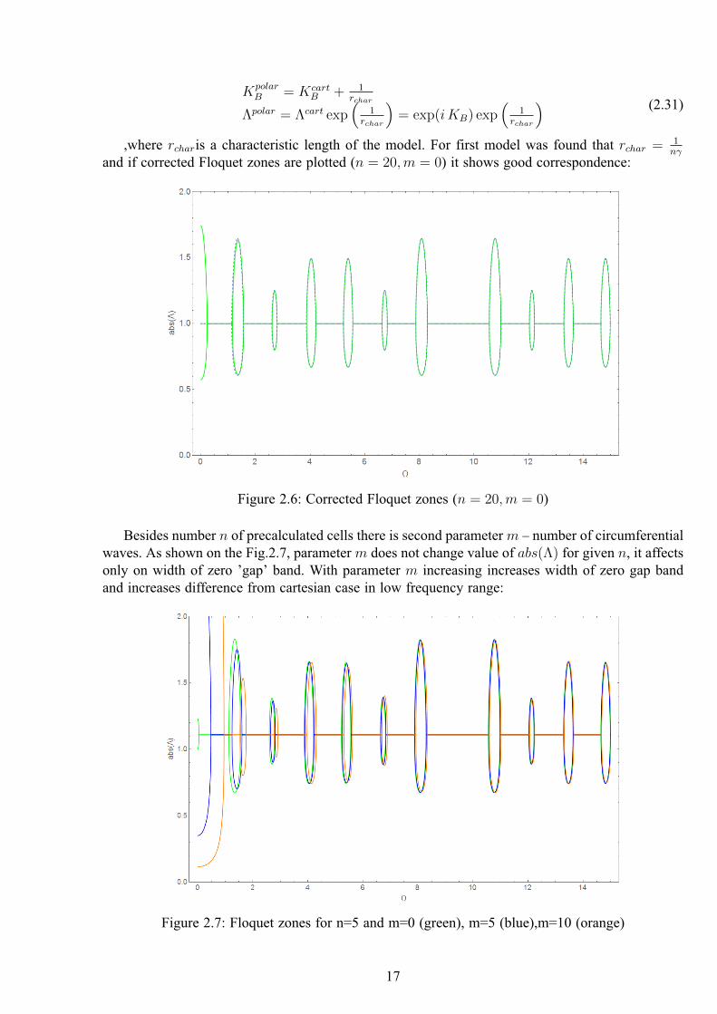
𝐾𝑝𝑜𝑙𝑎𝑟𝐵 = 𝐾𝑐𝑎𝑟𝑡

𝐵 + 1𝑟𝑐ℎ𝑎𝑟

Λ𝑝𝑜𝑙𝑎𝑟 = Λ𝑐𝑎𝑟𝑡 exp(

1𝑟𝑐ℎ𝑎𝑟

)= exp(𝑖𝐾𝐵) exp

(1

𝑟𝑐ℎ𝑎𝑟

) (2.31)

,where 𝑟𝑐ℎ𝑎𝑟is a characteristic length of the model. For first model was found that 𝑟𝑐ℎ𝑎𝑟 = 1𝑛𝛾

and if corrected Floquet zones are plotted (𝑛 = 20,𝑚 = 0) it shows good correspondence:

Figure 2.6: Corrected Floquet zones (𝑛 = 20,𝑚 = 0)

Besides number 𝑛 of precalculated cells there is second parameter 𝑚 – number of circumferentialwaves. As shown on the Fig.2.7, parameter 𝑚 does not change value of 𝑎𝑏𝑠(Λ) for given 𝑛, it affectsonly on width of zero ’gap’ band. With parameter 𝑚 increasing increases width of zero gap bandand increases difference from cartesian case in low frequency range:

Figure 2.7: Floquet zones for n=5 and m=0 (green), m=5 (blue),m=10 (orange)

17

As seen, main patterns, found for cartesian case are preserved for infinite waveguide case inpolar coordinates. But one should consider each case individually, because form of fundamentalsolution is different for each coordinate system (for example, exponents in cartesian coordinates,Bessel and Hankel functions in polar).

2.2.2 Finite structures

Every finite structure can be considered as series of a ’unit’ symmetrical periodicity cell (seeFig 1.2). In order to find eigenfrequencies interfacial conditions should be stated:

𝑢1(𝜆) = 𝑢2(𝜆)𝑢′

1(𝜆) = 𝛼𝛽𝑢′2(𝜆)

𝑢2((1 + 𝛾)𝜆) = 𝑢3((1 + 𝛾)𝜆)𝛼𝛽𝑢′

2((1 + 𝛾)𝜆) = 𝑢′3((1 + 𝛾)𝜆)

(2.32)

And two types of boundary conditions (see App.A for Hamilton’s principle explanation):

𝑢1(𝜆/2) = 0𝑢3((3/2 + 𝛾)𝜆) = 0

(2.33)

−𝑢′1(𝜆/2) = 0

𝑢′3((3/2 + 𝛾)𝜆) = 0

(2.34)

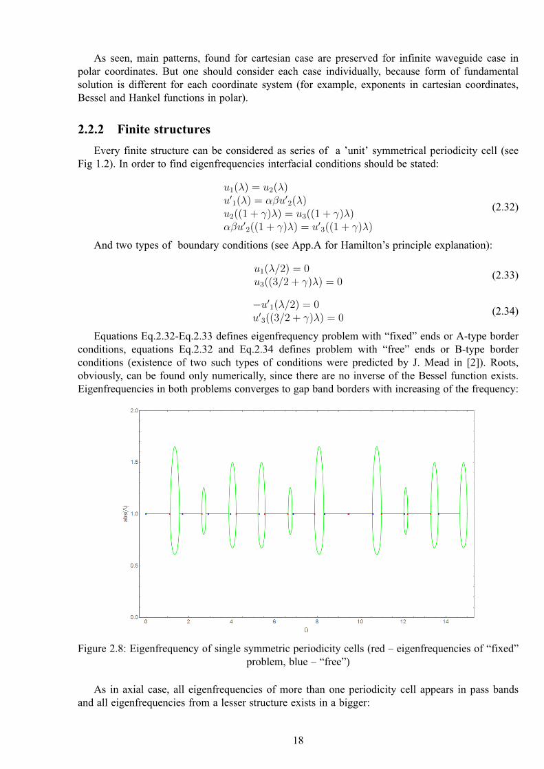
Equations Eq.2.32-Eq.2.33 defines eigenfrequency problem with “fixed” ends or A-type borderconditions, equations Eq.2.32 and Eq.2.34 defines problem with “free” ends or B-type borderconditions (existence of two such types of conditions were predicted by J. Mead in [2]). Roots,obviously, can be found only numerically, since there are no inverse of the Bessel function exists.Eigenfrequencies in both problems converges to gap band borders with increasing of the frequency:

Figure 2.8: Eigenfrequency of single symmetric periodicity cells (red – eigenfrequencies of “fixed”problem, blue – “free”)

As in axial case, all eigenfrequencies of more than one periodicity cell appears in pass bandsand all eigenfrequencies from a lesser structure exists in a bigger:

18

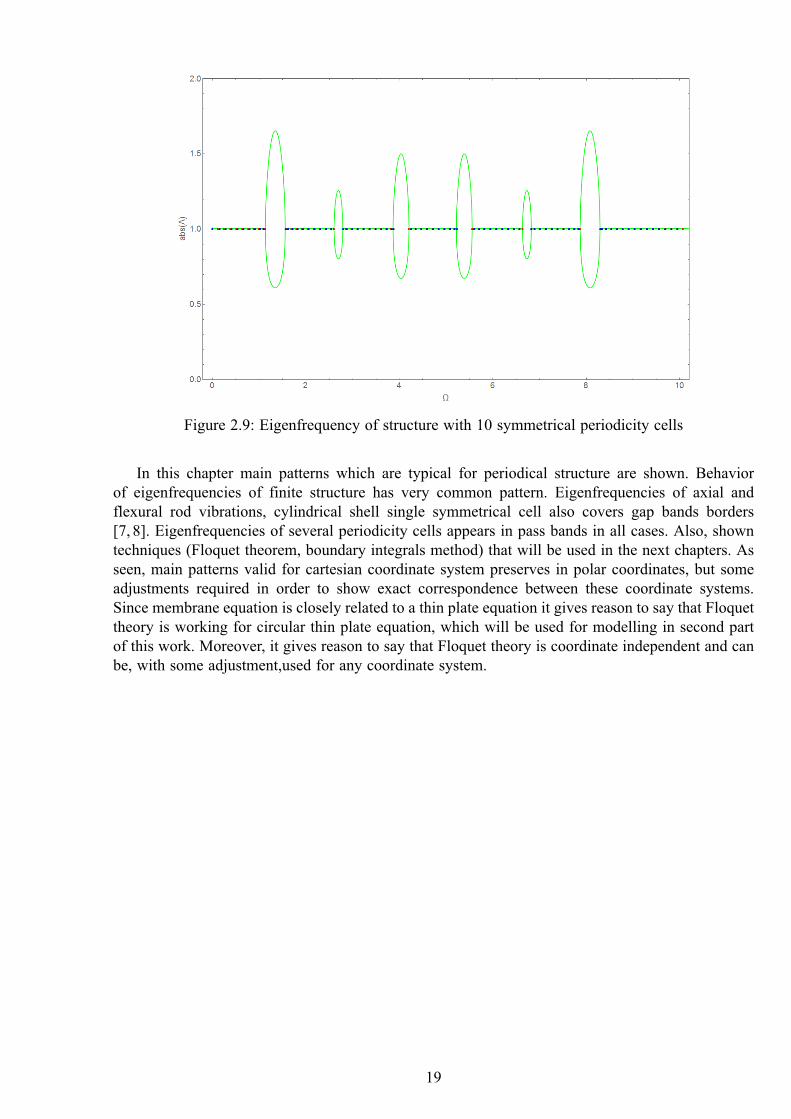
Figure 2.9: Eigenfrequency of structure with 10 symmetrical periodicity cells

In this chapter main patterns which are typical for periodical structure are shown. Behaviorof eigenfrequencies of finite structure has very common pattern. Eigenfrequencies of axial andflexural rod vibrations, cylindrical shell single symmetrical cell also covers gap bands borders[7, 8]. Eigenfrequencies of several periodicity cells appears in pass bands in all cases. Also, showntechniques (Floquet theorem, boundary integrals method) that will be used in the next chapters. Asseen, main patterns valid for cartesian coordinate system preserves in polar coordinates, but someadjustments required in order to show exact correspondence between these coordinate systems.Since membrane equation is closely related to a thin plate equation it gives reason to say that Floquettheory is working for circular thin plate equation, which will be used for modelling in second partof this work. Moreover, it gives reason to say that Floquet theory is coordinate independent and canbe, with some adjustment,used for any coordinate system.

19

Chapter 3

Bernoulli-Euler curved beam model

In this chapter a simplified model of a torque vibration isolator is considered. Methods fromprevious chapter (Floquet theorem, boundary integrals method) have broad range of applicability.In this chapter all these methods are used for more complicated case of system of differentialequations. This chapter has theoretical and practical goals. Practical goal is to build first model oftorque vibration isolator in the form of a system of a differential equations. Theoretical goal is toshow the difference between the picture of Floquet zones of a single differential equation and asystem of differential equations. In order to achieve that, methods, considered in Ch.2 are expandedand full range of tools for system of differential equations is obtained.

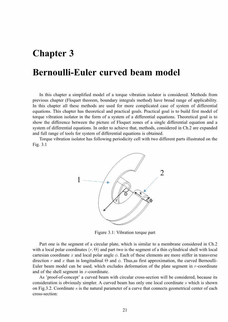
Torque vibration isolator has following periodicity cell with two different parts illustrated on theFig. 3.1

Figure 3.1: Vibration torque part

Part one is the segment of a circular plate, which is similar to a membrane considered in Ch.2with a local polar coordinates (𝑟,Θ) and part two is the segment of a thin cylindrical shell with localcartesian coordinate 𝑥 and local polar angle 𝜑. Each of these elements are more stiffer in transversedirection 𝑟 and 𝑥 than in longitudinal Θ and 𝜑. Thus,as first approximation, the curved Bernoulli-Euler beam model can be used, which excludes deformation of the plate segment in 𝑟-coordinateand of the shell segment in 𝑥-coordinate.

As ’proof-of-concept’ a curved beam with circular cross-section will be considered, because itsconsideration is obviously simpler. A curved beam has only one local coordinate 𝑠 which is shownon Fig.3.2. Coordinate 𝑠 is the natural parameter of a curve that connects geometrical center of eachcross-section:

21

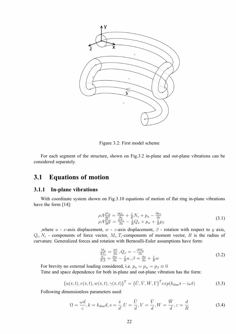
Figure 3.2: First model scheme

For each segment of the structure, shown on Fig.3.2 in-plane and out-plane vibrations can beconsidered separately.

3.1 Equations of motion

3.1.1 In-plane vibrations

With coordinate system shown on Fig.3.10 equations of motion of flat ring in-plane vibrationshave the form [14]:

𝜌𝐴𝜕2𝑢𝜕𝑡2

= 𝜕𝑄𝑥

𝜕𝑠+ 1

𝑅𝑁𝑧 + 𝑝𝑢 − 𝜕𝑝𝛽

𝜕𝑠

𝜌𝐴𝜕2𝑤𝜕𝑡2

= 𝜕𝑁𝑧

𝜕𝑠− 1

𝑅𝑄𝑥 + 𝑝𝑤 + 1

𝑅𝑝𝛽

(3.1)

,where 𝑢 - 𝑥-axis displacement, 𝑤 - 𝑧-axis displacement, 𝛽 - rotation with respect to 𝑦 axis,𝑄𝑖, 𝑁𝑖 - components of force vector, 𝑀𝑖, 𝑇𝑖-components of moment vector, 𝑅 is the radius ofcurvature. Generalized forces and rotation with Bernoulli-Euler assumptions have form:

𝑀𝑦

𝐸𝐼𝑦= 𝜕𝛽

𝜕𝑠, 𝑄𝑥 = −𝜕𝑀𝑦

𝜕𝑠𝑁𝑧

𝐸𝐴= 𝜕𝑤

𝜕𝑠− 1

𝑅𝑢 , 𝛽 = 𝜕𝑢

𝜕𝑠+ 1

𝑅𝑤

(3.2)

For brevity no external loading considered, i.e. 𝑝𝑢 = 𝑝𝑤 = 𝑝𝛽 ≡ 0Time and space dependence for both in-plane and out-plane vibration has the form:

𝑢(𝑠, 𝑡), 𝑣(𝑠, 𝑡), 𝑤(𝑠, 𝑡), 𝛾(𝑠, 𝑡)𝑇 = , 𝑉 , ,Γ𝑇 𝑒𝑥𝑝(𝑘dim𝑠− 𝑖𝜔𝑡) (3.3)

Following dimensionless parameters used:

Ω =𝜔𝑑

𝑐, 𝑘 = 𝑘dim𝑑, 𝑠 =

𝑠

𝑑, 𝑈 =

𝑑, 𝑉 =

𝑉

𝑑,𝑊 =

𝑑, 𝜀 =

𝑑

𝑅(3.4)

22

With time and space dependence Eq.3.3 and dimensionless parameters Eq.3.4substituted into thesystem Eq.3.1-Eq.3.2 following system is obtained:

𝑊(16k𝜀− k3𝜀

)+ 𝑈

(−k4 − 16𝜀2 + 16Ω2

)= 0

𝑈(−16k𝜀 + k3𝜀

)+ 𝑊

(16k2 + k2𝜀2 + 16Ω2

)= 0

(3.5)

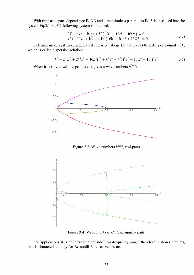
Determinant of system of algebraical linear equations Eq.3.5 gives 6th order polynomial in 𝑘,which is called dispersion relation:

𝑘6 + 𝑘4Ω2 + 2𝑘4𝜀2 − 16𝑘2Ω2 + 𝑘2𝜀4 − 𝑘2Ω2𝜀2 − 16Ω4 + 16Ω2𝜀2 (3.6)

When it is solved with respect to 𝑘 it gives 6 wavenumbers 𝑘(𝑖𝑛)𝑖 :

Figure 3.3: Wave numbers 𝑘(𝑖𝑛), real parts

Figure 3.4: Wave numbers 𝑘(𝑖𝑛), imaginary parts

For applications it is of interest to consider low-frequency range, therefore it shows pictures,that is characteristic only for Bernoulli-Euler curved beam:

23

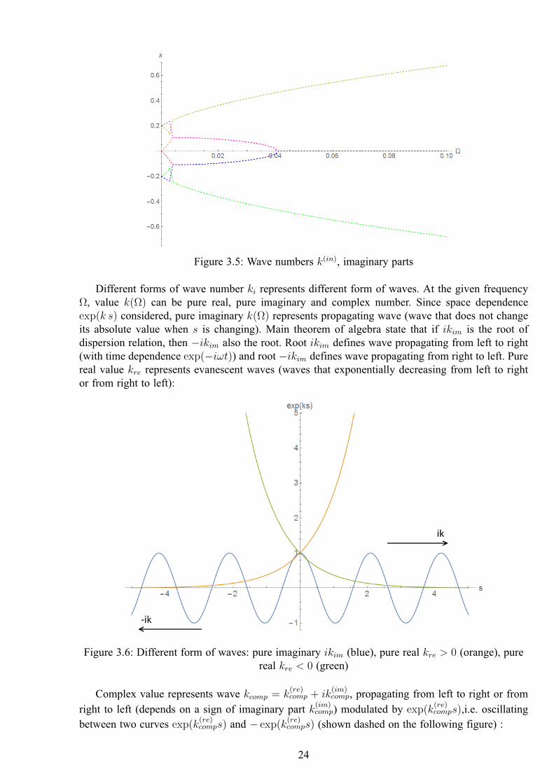
Figure 3.5: Wave numbers 𝑘(𝑖𝑛), imaginary parts

Different forms of wave number 𝑘𝑖 represents different form of waves. At the given frequencyΩ, value 𝑘(Ω) can be pure real, pure imaginary and complex number. Since space dependenceexp(𝑘 𝑠) considered, pure imaginary 𝑘(Ω) represents propagating wave (wave that does not changeits absolute value when 𝑠 is changing). Main theorem of algebra state that if 𝑖𝑘𝑖𝑚 is the root ofdispersion relation, then −𝑖𝑘𝑖𝑚 also the root. Root 𝑖𝑘𝑖𝑚 defines wave propagating from left to right(with time dependence exp(−𝑖𝜔𝑡)) and root −𝑖𝑘𝑖𝑚 defines wave propagating from right to left. Purereal value 𝑘𝑟𝑒 represents evanescent waves (waves that exponentially decreasing from left to rightor from right to left):

Figure 3.6: Different form of waves: pure imaginary 𝑖𝑘𝑖𝑚 (blue), pure real 𝑘𝑟𝑒 > 0 (orange), purereal 𝑘𝑟𝑒 < 0 (green)

Complex value represents wave 𝑘𝑐𝑜𝑚𝑝 = 𝑘(𝑟𝑒)𝑐𝑜𝑚𝑝 + 𝑖𝑘

(𝑖𝑚)𝑐𝑜𝑚𝑝, propagating from left to right or from

right to left (depends on a sign of imaginary part 𝑘(𝑖𝑚)𝑐𝑜𝑚𝑝) modulated by exp(𝑘

(𝑟𝑒)𝑐𝑜𝑚𝑝𝑠),i.e. oscillating

between two curves exp(𝑘(𝑟𝑒)𝑐𝑜𝑚𝑝𝑠) and − exp(𝑘

(𝑟𝑒)𝑐𝑜𝑚𝑝𝑠) (shown dashed on the following figure) :

24

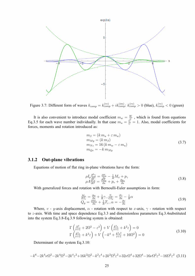
Figure 3.7: Different form of waves 𝑘𝑐𝑜𝑚𝑝 = 𝑘(𝑟𝑒)𝑐𝑜𝑚𝑝 + 𝑖𝑘

(𝑖𝑚)𝑐𝑜𝑚𝑝: 𝑘

(𝑟𝑒)𝑐𝑜𝑚𝑝 > 0 (blue), 𝑘(𝑟𝑒)

𝑐𝑜𝑚𝑝 < 0 (green)

It is also convenient to introduce modal coefficient 𝑚𝑤 = 𝑊𝑈

, which is found from equationsEq.3.5 for each wave number individually. In that case 𝑚𝑢 = 𝑈

𝑈= 1. Also, modal coefficients for

forces, moments and rotation introduced as:

𝑚𝛽 = (𝑘𝑚𝑢 + 𝜀𝑚𝑤)𝑚𝑀𝑦 = (𝑘𝑚𝛽)𝑚𝑁𝑧 = 16 (𝑘𝑚𝑤 − 𝜀𝑚𝑢)𝑚𝑄𝑥 = −𝑘𝑚𝑀𝑦

(3.7)

3.1.2 Out-plane vibrations

Equations of motion of flat ring in-plane vibrations have the form:

𝜌𝐼𝑝𝜕2𝛾𝜕𝑡2

= 𝜕𝑇𝑧

𝜕𝑠− 1

𝑅𝑀𝑥 + 𝑝𝛾

𝜌𝐴𝜕2𝑣𝜕𝑡2

= 𝜕𝑄𝑦

𝜕𝑠+ 𝑝𝑣 + 𝜕𝑝𝛼

𝜕𝑠

(3.8)

With generalized forces and rotation with Bernoulli-Euler assumptions in form:

𝑀𝑥

𝐸𝐼𝑥= 𝜕𝛼

𝜕𝑠+ 1

𝑅𝛾 , 𝑇𝑧

𝐺𝐼𝑝= 𝜕𝛾

𝜕𝑠− 1

𝑅𝛼

𝑄𝑦 = 𝜕𝑀𝑥

𝜕𝑠+ 1

𝑅𝑇𝑧 , 𝛼 = −𝜕𝑣

𝜕𝑠

(3.9)

Where, 𝑣 - 𝑦-axis displacement, 𝛼 - rotation with respect to 𝑥-axis, 𝛾 - rotation with respectto 𝑧-axis. With time and space dependence Eq.3.3 and dimensionless parameters Eq.3.4substitutedinto the system Eq.3.8-Eq.3.9 following system is obtained:

Γ(

𝑘2

𝜈+1+ 2Ω2 − 𝜀2

)+ 𝑉

(𝑘2𝜀𝜈+1

+ 𝑘2𝜀)

= 0

Γ(

𝑘2𝜀𝜈+1

+ 𝑘2𝜀)

+ 𝑉(−𝑘4 + 𝑘2𝜀2

𝜈+1+ 16Ω2

)= 0

(3.10)

Determinant of the system Eq.3.10:

−𝑘6−2𝑘4𝜈Ω2−2𝑘4Ω2−2𝑘4𝜀2+16𝑘2Ω2−𝑘2𝜀4+2𝑘2Ω2𝜀2+32𝜈Ω4+32Ω4−16𝜈Ω2𝜀2−16Ω2𝜀2 (3.11)

25

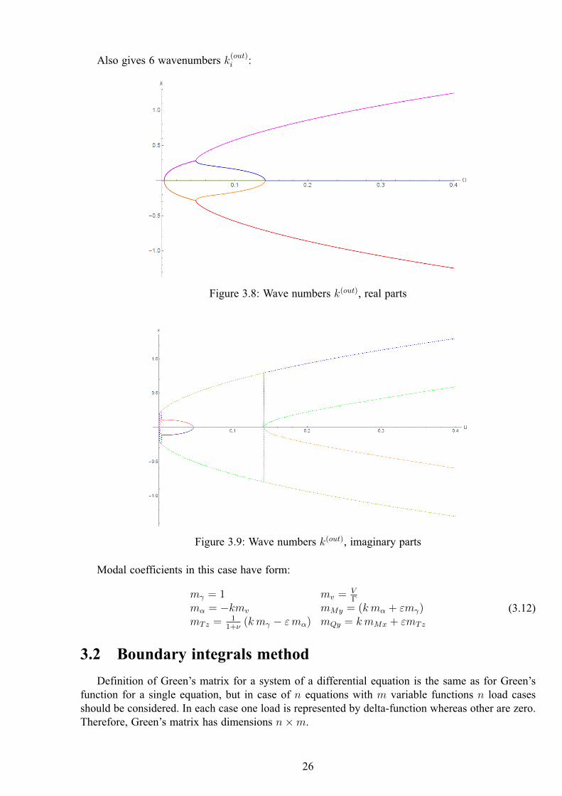
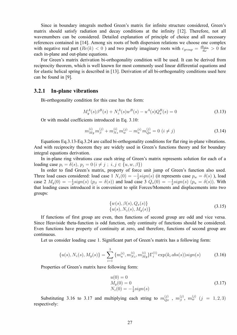
Also gives 6 wavenumbers 𝑘(𝑜𝑢𝑡)𝑖 :

Figure 3.8: Wave numbers 𝑘(𝑜𝑢𝑡), real parts

Figure 3.9: Wave numbers 𝑘(𝑜𝑢𝑡), imaginary parts

Modal coefficients in this case have form:

𝑚𝛾 = 1 𝑚𝑣 = 𝑉Γ

𝑚𝛼 = −𝑘𝑚𝑣 𝑚𝑀𝑦 = (𝑘𝑚𝛼 + 𝜀𝑚𝛾)𝑚𝑇𝑧 = 1

1+𝜈(𝑘𝑚𝛾 − 𝜀𝑚𝛼) 𝑚𝑄𝑦 = 𝑘𝑚𝑀𝑥 + 𝜀𝑚𝑇𝑧

(3.12)

3.2 Boundary integrals method

Definition of Green’s matrix for a system of a differential equation is the same as for Green’sfunction for a single equation, but in case of 𝑛 equations with 𝑚 variable functions 𝑛 load casesshould be considered. In each case one load is represented by delta-function whereas other are zero.Therefore, Green’s matrix has dimensions 𝑛×𝑚.

26

Since in boundary integrals method Green’s matrix for infinite structure considered, Green’smatrix should satisfy radiation and decay conditions at the infinity [12]. Therefore, not allwavenumbers can be considered. Detailed explanation of principle of choice and all necessaryreferences contained in [14]. Among six roots of both dispersion relations we choose one complexwith negative real part (𝑅𝑒(𝑘) < 0 ) and two purely imaginary roots with 𝑐𝑔𝑟𝑜𝑢𝑝 = 𝑑𝑘𝑑𝑖𝑛

𝑑𝜔> 0 for

each in-plane and out-plane equations.For Green’s matrix derivation bi-orthogonality condition will be used. It can be derived from

reciprocity theorem, which is well known for most commonly used linear differential equations andfor elastic helical spring is described in [13]. Derivation of all bi-orthogonality conditions used herecan be found in [9].

3.2.1 In-plane vibrations

Bi-orthogonality condition for this case has the form:

𝑀𝐴𝑦 (𝑠)𝛽𝐵(𝑠) + 𝑁𝐴

𝑧 (𝑠)𝑤𝐵(𝑠) − 𝑢𝐴(𝑠)𝑄𝐵𝑥 (𝑠) = 0 (3.13)

Or with modal coefficients introduced in Eq. 3.10:

𝑚(𝑖)𝑀𝑦 𝑚

(𝑗)𝛽 + 𝑚

(𝑖)𝑁𝑧 𝑚

(𝑗)𝑤 −𝑚(𝑖)

𝑢 𝑚(𝑗)𝑄𝑥 = 0 (𝑖 = 𝑗) (3.14)

Equations Eq.3.13-Eq.3.24 are called bi-orthogonality conditions for flat ring in-plane vibrations.And with reciprocity theorem they are widely used in Green’s functions theory and for boundaryintegral equations derivation.

In in-plane ring vibrations case each string of Green’s matrix represents solution for each of aloading case 𝑝𝑖 = 𝛿(𝑠), 𝑝𝑗 = 0 (𝑖 = 𝑗 ; 𝑖, 𝑗 ∈ 𝑢,𝑤, 𝛽)

In order to find Green’s matrix, property of force unit jump of Green’s function also used.Three load cases considered: load case 1 𝑁𝑧(0) = −1

2𝑠𝑖𝑔𝑛(𝑠) (it represents case 𝑝𝑤 = 𝛿(𝑠) ), load

case 2 𝑀𝑦(0) = −12𝑠𝑖𝑔𝑛(𝑠) (𝑝𝛽 = 𝛿(𝑠)) and load case 3 𝑄𝑥(0) = −1

2𝑠𝑖𝑔𝑛(𝑠) (𝑝𝑢 = 𝛿(𝑠)). With

that loading cases introduced it is convenient to split Forces/Moments and displacements into twogroups:

𝑤(𝑠), 𝛽(𝑠), 𝑄𝑥(𝑠)𝑢(𝑠), 𝑁𝑧(𝑠),𝑀𝑦(𝑠)

(3.15)

If functions of first group are even, then functions of second group are odd and vice versa.Since Heaviside theta-function is odd function, only continuity of functions should be considered.Even functions have property of continuity at zero, and therefore, functions of second group arecontinuous.

Let us consider loading case 1. Significant part of Green’s matrix has a following form:

𝑢(𝑠), 𝑁𝑧(𝑠),𝑀𝑦(𝑠) =3∑

𝑖=1

𝑚(𝑖)𝑢 ,𝑚

(𝑖)𝑁𝑧,𝑚

(𝑖)𝑀𝑦Γ

(1)𝑖 exp(𝑘𝑖 𝑎𝑏𝑠(𝑠))𝑠𝑖𝑔𝑛(𝑠) (3.16)

Properties of Green’s matrix have following form:

𝑢(0) = 0𝑀𝑦(0) = 0𝑁𝑧(0) = −1

2𝑠𝑖𝑔𝑛(𝑠)

(3.17)

Substituting 3.16 to 3.17 and multiplying each string to 𝑚(𝑗)𝑄𝑥 , 𝑚

(𝑗)𝛽 , 𝑚

(𝑗)𝑤 (𝑗 = 1, 2, 3)

respectively:

27

3∑𝑖=1

Γ(1)𝑖 𝑚

(𝑖)𝑢 𝑚

(𝑗)𝑄𝑥 = 0

3∑𝑖=1

Γ(1)𝑖 𝑚

(𝑖)𝑀𝑦𝑚

(𝑗)𝛽 = 0

3∑𝑖=1

Γ(1)𝑖 𝑚𝑁𝑧

(𝑖)𝑚(𝑗)𝑤 = −1

2

(3.18)

Summing all equations in 3.18:

3∑𝑖=1

Γ(1)𝑖 (𝑚(𝑖)

𝑢 𝑚(𝑗)𝑄𝑥 + 𝑚

(𝑖)𝑀𝑦 𝑚

(𝑗)𝛽 + 𝑚

(𝑖)𝑁𝑧 𝑚

(𝑗)𝑤 ) = −1

2(3.19)

Expression in brackets is exactly bi-orthogonal condition 3.24 and it is not zero only when 𝑖 = 𝑗.Thus one can obtain explicit form of each coefficient Γ

(1)𝑖 .

In same way all Green’s matrix coefficient entries can be found as:

Γ(𝑖𝑛)(1)𝑖 = −1

2𝑚

(𝑖)𝑤

𝑚(𝑖)𝑀𝑦 𝑚

(𝑖)𝛽 +𝑚𝑁𝑧𝑖 𝑚

(𝑖)𝑤 −𝑚

(𝑖)𝑢 𝑚

(𝑖)𝑄𝑥

Γ(𝑖𝑛)(2)𝑖 = −1

2

𝑚(𝑖)𝛽

𝑚(𝑖)𝑀𝑦 𝑚

(𝑖)𝛽 +𝑚𝑁𝑧𝑖 𝑚

(𝑖)𝑤 −𝑚

(𝑖)𝑢 𝑚

(𝑖)𝑄𝑥

Γ(𝑖𝑛)(3)𝑖 = 1

2𝑚

(𝑖)𝑢

𝑚(𝑖)𝑀𝑦 𝑚𝛽𝑖+𝑚𝑁𝑧𝑖 𝑚

(𝑖)𝑤 −𝑚

(𝑖)𝑢 𝑚

(𝑖)𝑄𝑥

(3.20)

After coefficients found green matrix formed as (on example of loading case 1):

𝐺𝑖𝑛1 (𝑠, 𝑠0) = 𝑢(𝑛)(𝑠), 𝑤(𝑛)(𝑠), 𝛽(𝑛)(𝑠), 𝑄

(𝑛)𝑥 (𝑠), 𝑁

(𝑛)𝑧 (𝑠),𝑀

(𝑛)𝑦 (𝑠) =

3∑𝑖=1

𝑠𝑖𝑔𝑛(𝑠)𝑚(𝑖)𝑢 ,𝑚

(𝑖)𝑤 ,𝑚

(𝑖)𝛽 ,𝑚

(𝑖)𝑄𝑥, 𝑠𝑖𝑔𝑛(𝑠)𝑚𝑁𝑧𝑖, 𝑠𝑖𝑔𝑛(𝑠)𝑚

(𝑖)𝑀𝑦Γ(𝑖𝑛)

(1)𝑖 exp(𝑘𝑖𝑛

𝑖 𝑎𝑏𝑠(𝑠− 𝑠0))

(3.21)After Green’s matrix found, one can obtain displacement, expressed in terms of Green’s matrix

(analogous to 2.13) in same way as it done in App.B. It can be written as ( [13]):

𝛿1𝑛𝑤(𝑠0) + 𝛿2𝑛𝛽(𝑠0) + 𝛿3𝑛𝑢(𝑠0) =[𝐺𝑖𝑛

𝑛 (𝑠, 𝑠0). 𝑄𝑥(𝑠), 𝑁𝑧(𝑠),𝑀𝑦(𝑠),−𝑢(𝑠),−𝑤(𝑠),−𝛽(𝑠)]𝑠=𝑏

𝑠=𝑎(3.22)

,where 𝛿𝑖𝑗 -Kronecker’s delta and . - dot product of two vectors. Equations Eq.?? calledboundary integrals for ring in-plane vibrations.

3.2.2 Out-plane vibrations

In same way, with three loading cases: load case 1 𝑄𝑦(0) = −12𝑠𝑖𝑔𝑛(𝑠) (𝑝𝑢 = 𝛿(𝑠) ), load case

2 𝑇𝑧(0) = −12𝑠𝑖𝑔𝑛(𝑠) (𝑝𝛾 = 𝛿(𝑠)) and load case 3 𝑀𝑥(0) = −1

2𝑠𝑖𝑔𝑛(𝑠) (𝑝𝛼 = 𝛿(𝑠)).

Two groups of functions:

𝑣(𝑠), 𝛾(𝑠),𝑀𝑥(𝑠)𝛼(𝑠), 𝑇𝑧(𝑠), 𝑄𝑦(𝑠)

(3.23)

And bi-orthogonality condition:

𝑚(𝑖)𝑇𝑧 𝑚

(𝑗)𝛾 + 𝑚

(𝑖)𝑄𝑦 𝑚

(𝑗)𝑣 −𝑚(𝑖)

𝛼 𝑚(𝑗)𝑀𝑥 = 0 (𝑖 = 𝑗) (3.24)

One can obtain Green’s matrix coefficients in form:

28

Γ(𝑜𝑢𝑡)(1)𝑖 = −1

2𝑚

(𝑖)𝑣

𝑚(𝑖)𝑇𝑧 𝑚

(𝑖)𝛾 +𝑚

(𝑖)𝑄𝑦 𝑚

(𝑖)𝑣 −𝑚

(𝑖)𝛼 𝑚

(𝑖)𝑀𝑥

Γ(𝑜𝑢𝑡)(2)𝑖 = −1

2

𝑚(𝑖)𝛾

𝑚(𝑖)𝑇𝑧 𝑚

(𝑖)𝛾 +𝑚

(𝑖)𝑄𝑦 𝑚

(𝑖)𝑣 −𝑚

(𝑖)𝛼 𝑚

(𝑖)𝑀𝑥

Γ(𝑜𝑢𝑡)(3)𝑖 = 1

2𝑚

(𝑖)𝛼

𝑚(𝑖)𝑇𝑧 𝑚

(𝑖)𝛾 +𝑚

(𝑖)𝑄𝑦 𝑚

(𝑖)𝑣 −𝑚

(𝑖)𝛼 𝑚

(𝑖)𝑀𝑥

(3.25)

Green’s matrix in form:

𝐺𝑜𝑢𝑡1 (𝑠, 𝑠0) = 𝑣(𝑛)(𝑠), 𝛼(𝑛)(𝑠), 𝛾(𝑛)(𝑠), 𝑄

(𝑛)𝑦 (𝑠),𝑀

(𝑛)𝑧 (𝑠), 𝑇

(𝑛)𝑧 (𝑠) =

3∑𝑖=1

𝑚(𝑖)𝑣 , 𝑠𝑖𝑔𝑛(𝑠)𝑚

(𝑖)𝛼 ,𝑚𝛾𝑖, 𝑠𝑖𝑔𝑛(𝑠)𝑚

(𝑖)𝑄𝑦,𝑚

(𝑖)𝑀𝑥, 𝑠𝑖𝑔𝑛(𝑠)𝑚

(𝑖)𝑇𝑧Γ(𝑜𝑢𝑡)

(1)𝑖 exp(𝑘𝑜𝑢𝑡

𝑖 𝑎𝑏𝑠(𝑠− 𝑠0))

(3.26)And boundary equations in form:

𝛿1𝑛𝑣(𝑠0) + 𝛿2𝑛𝛾(𝑠0) + 𝛿3𝑛𝛼(𝑠0) =[𝐺𝑜𝑢𝑡

𝑛 (𝑠, 𝑠0). 𝑄𝑦(𝑠),𝑀𝑥(𝑠), 𝑇 𝑧(𝑠),−𝑢(𝑠),−𝛼(𝑠),−𝛾(𝑠)]𝑠=𝑏

𝑠=𝑎(3.27)

3.3 The benchmark periodic structure

In order to validate the theory and the Wolfram Mathematica codes, an auxiliary problem hasbeen considered first.

3.3.1 Infinite periodic structure

With respect to natural coordinate 𝑠 ring can be considered as periodic structure shown onthe Fig.1.2. Similar problem was considered in [3] for a helical spring and flat ring, but it wasconsidered within Timoshenko beam theory. In this work, as stated above Bernoulli-Euler theoryconsidered.

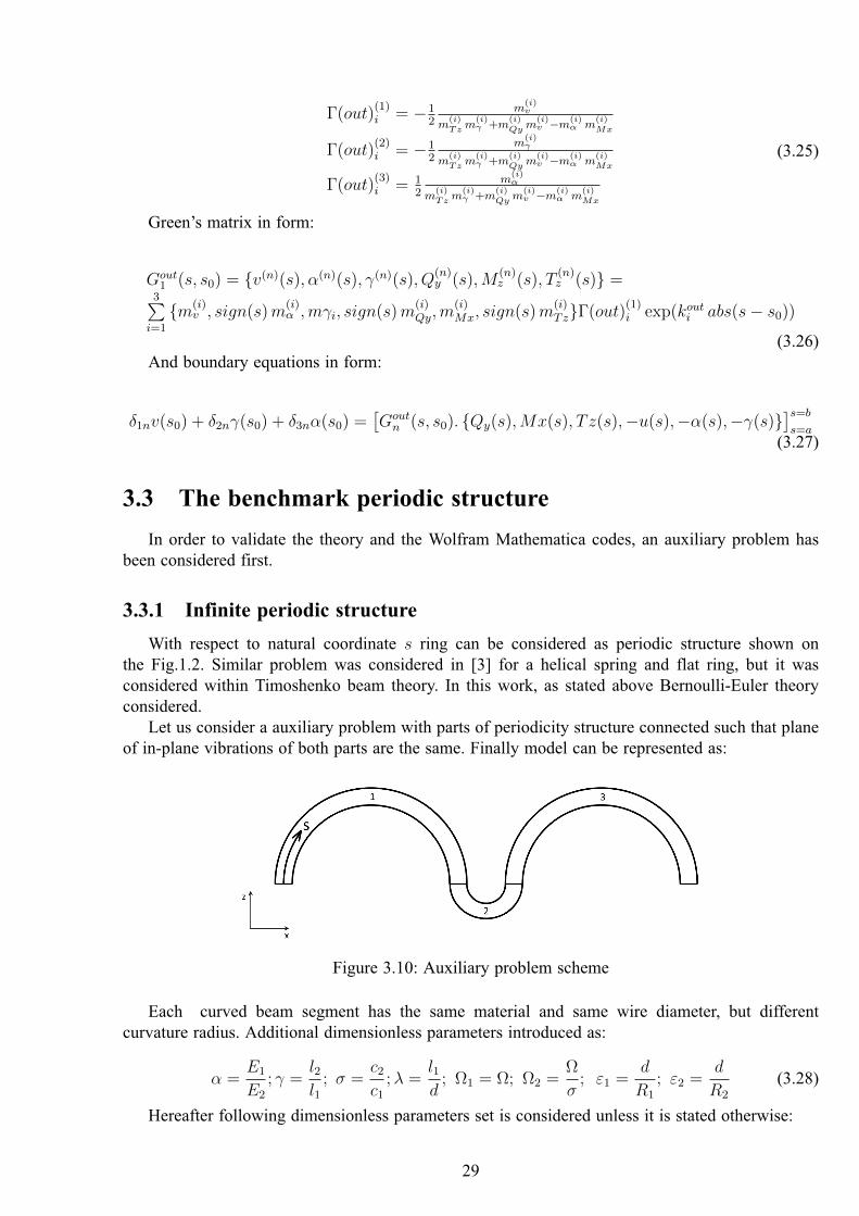
Let us consider a auxiliary problem with parts of periodicity structure connected such that planeof in-plane vibrations of both parts are the same. Finally model can be represented as:

Figure 3.10: Auxiliary problem scheme

Each curved beam segment has the same material and same wire diameter, but differentcurvature radius. Additional dimensionless parameters introduced as:

𝛼 =𝐸1

𝐸2

; 𝛾 =𝑙2𝑙1

; 𝜎 =𝑐2𝑐1

;𝜆 =𝑙1𝑑

; Ω1 = Ω; Ω2 =Ω

𝜎; 𝜀1 =

𝑑

𝑅1

; 𝜀2 =𝑑

𝑅2

(3.28)

Hereafter following dimensionless parameters set is considered unless it is stated otherwise:

29

𝛼 = 1; 𝛾 = 0.5; 𝜎 = 1;𝜆 = 5; 𝜀1 = 0.2; 𝜀2 = 0.02 (3.29)

As in the case of axial and flexural beam vibrations Floquet theory can be used. Followingnotation used:

𝑑𝑖𝑠𝑝𝑖(𝑠) = 𝑤𝑖(𝑠), 𝛽𝑖(𝑠), 𝑢𝑖(𝑠), 𝑣𝑖(𝑠), 𝛾𝑖(𝑠), 𝛼𝑖(𝑠)𝑓𝑜𝑟𝑐𝑒𝑖(𝑠) = 1

𝐸𝑖𝐼(𝑖)𝑥

𝑄(𝑖)𝑥 (𝑠), 𝑁

(𝑖)𝑧 (𝑠),𝑀

(𝑖)𝑦 (𝑠), 𝑄

(𝑖)𝑦 (𝑠),𝑀

(𝑖)𝑥 (𝑠), 𝑇

(𝑖)𝑧 (𝑠) (3.30)

Let us consider three subsequent parts of ring. For each part of ring we define two set ofthree boundary integrals in form Eq.3.29 and Eq.3.35 (totally, 6*6=36 equations) and additionallyinterfacial conditions (4*6=24 equations):

𝑤1(1) = 𝑤2(1) ; 𝛽1(1) = 𝛽2(1) ;𝑢1(1) = 𝑢2(1)𝛾1(1) = 𝛾2(1) ; 𝑣1(1) = 𝑣2(1) ;𝛼1(1) = 𝛼2(1)

𝑁(1)𝑧 (1) = 𝛼𝑝𝑎𝑟 𝑁

(2)𝑧 (1) ;𝑀

(1)𝑦 (1) = 𝛼𝑝𝑎𝑟 𝑀

(2)𝑦 (1) ;𝑄

(1)𝑥 (1) = 𝛼𝑝𝑎𝑟 𝑄

(2)𝑥 (1)

𝑇(1)𝑧 (1) = 𝛼𝑝𝑎𝑟 𝑇

(2)𝑧 (1) ;𝑄

(1)𝑦 (1) = 𝛼𝑝𝑎𝑟 𝑄

(2)𝑦 (1) ;𝑀

(1)𝑥 (1) = 𝛼𝑝𝑎𝑟 𝑀

(2)𝑥 (1)

𝑤2(1 + 𝛾𝑝𝑎𝑟) = 𝑤3(1 + 𝛾𝑝𝑎𝑟) ; 𝛽2(1 + 𝛾𝑝𝑎𝑟) = 𝛽3(1 + 𝛾𝑝𝑎𝑟) ;𝑢2(1 + 𝛾𝑝𝑎𝑟) = 𝑢3(1 + 𝛾𝑝𝑎𝑟)𝛾2(1 + 𝛾𝑝𝑎𝑟) = 𝛾3(1 + 𝛾𝑝𝑎𝑟) ; 𝑣2(1 + 𝛾𝑝𝑎𝑟) = 𝑣3(1 + 𝛾𝑝𝑎𝑟) ;𝛼2(1 + 𝛾𝑝𝑎𝑟) = 𝛼3(1 + 𝛾𝑝𝑎𝑟)

𝑁(2)𝑧 (1 + 𝛾𝑝𝑎𝑟) = 𝛼𝑝𝑎𝑟 𝑁

(3)𝑧 (1 + 𝛾𝑝𝑎𝑟) ;𝑀

(2)𝑦 (1 + 𝛾𝑝𝑎𝑟) = 𝛼𝑝𝑎𝑟 𝑀

(3)𝑦 (1 + 𝛾𝑝𝑎𝑟)

𝑄(2)𝑥 (1 + 𝛾𝑝𝑎𝑟) = 𝛼𝑝𝑎𝑟 𝑄

(3)𝑥 (1 + 𝛾𝑝𝑎𝑟)

𝑇(2)𝑧 (1 + 𝛾𝑝𝑎𝑟) = 𝛼𝑝𝑎𝑟 𝑇

(3)𝑧 (1 + 𝛾𝑝𝑎𝑟) ;𝑄

(2)𝑦 (1 + 𝛾𝑝𝑎𝑟) = 𝛼𝑝𝑎𝑟 𝑄

(3)𝑦 (1 + 𝛾𝑝𝑎𝑟)

𝑀(2)𝑥 (1 + 𝛾𝑝𝑎𝑟) = 𝛼𝑝𝑎𝑟 𝑀

(3)𝑥 (1 + 𝛾𝑝𝑎𝑟)

(3.31a)Or in vector form:

𝑑𝑖𝑠𝑝1(1) = 𝑑𝑖𝑠𝑝2(1)𝑓𝑜𝑟𝑐𝑒1(1) = 𝛼 𝑓𝑜𝑟𝑐𝑒2(1)𝑑𝑖𝑠𝑝2(1 + 𝛾) = 𝑑𝑖𝑠𝑝3(1 + 𝛾)𝛼𝑓𝑜𝑟𝑐𝑒2(1 + 𝛾) = 𝑓𝑜𝑟𝑐𝑒3(1 + 𝛾)

(3.31b)

And Floquet periodicity conditions (2*6=12 equations):

𝑢1(0) = Λ𝑢3(1 + 𝛾); 𝑣1(0) = Λ𝑢3(1 + 𝛾); 𝑤1(0) = Λ𝑢3(1 + 𝛾)𝛼1(0) = Λ𝛼3(1 + 𝛾); 𝛽1(0) = Λ 𝛽3(1 + 𝛾); 𝛾1(0) = Λ 𝛾3(1 + 𝛾)

𝑀(1)𝑥 (0) = Λ𝑀

(3)𝑥 (1 + 𝛾); 𝑀

(1)𝑦 (0) = Λ𝑀

(3)𝑦 (1 + 𝛾); 𝑇

(1)𝑧 (0) = Λ𝑇

(3)𝑧 (1 + 𝛾)

𝑄(1)𝑥 (0) = Λ𝑄

(3)𝑥 (1 + 𝛾); 𝑄

(1)𝑦 (0) = Λ𝑄

(3)𝑦 (1 + 𝛾); 𝑁

(1)𝑧 (0) = Λ𝑁

(3)𝑧 (1 + 𝛾)

(3.32a)

Or in vector form:

𝑑𝑖𝑠𝑝1(0) = Λ 𝑑𝑖𝑠𝑝3(1 + 𝛾)𝑓𝑜𝑟𝑐𝑒1(0) = Λ 𝑓𝑜𝑟𝑐𝑒3(1 + 𝛾) (3.32b)

Boundary integrals with conditions Eq.3.31a-Eq.3.32b defines homogenous system ofalgebraical equations with respect to unknown displacements and forces on borders of the ringparts. Let 𝐷(Λ,Ω) be the determinant of this system. 𝐷(Λ,Ω) is the twelfth order polynomialin Λ , which defines stop- and pass-bands. It should be empathized, that determinant 𝐷(Λ,Ω)

30

factorizes in two sixth order polynomials in Λ : in- and out- plane vibrations part, i.e. 𝐷(Λ,Ω) =𝐷𝑖𝑛(Λ,Ω) *𝐷𝑜𝑢𝑡(Λ,Ω). Therefore these two parts can be considered independently.

It should be noted that both of determinants 𝐷𝑖𝑛(Λ,Ω) and 𝐷𝑜𝑢𝑡(Λ,Ω) can be written in form:

𝐷*(Λ,Ω) = Λ6 + 𝑎5Λ5 + 𝑎4Λ

4 + 𝑎3Λ3 + 𝑎2Λ

2 + 𝑎1Λ + 1 (3.33)

It has two properties: 1.By Vieta theorem, since free term of polynomial 𝐷*(Λ,Ω) is 1, if Λ isa root of polynomial Eq.3.33, then Λ−1 is a root of polynomial too. 2. It has only even powers ofΩ as coefficients 𝑎𝑖 because no damping is considered.

For further consideration it is convenient to write 𝐷𝑖𝑛 as 𝐷𝑤,𝑢 with meaning of flexural-axialpart of a Floquet determinant. Also 𝐷𝑜𝑢𝑡 written as 𝐷𝛾,𝑣 with meaning of flexural-torsional part.

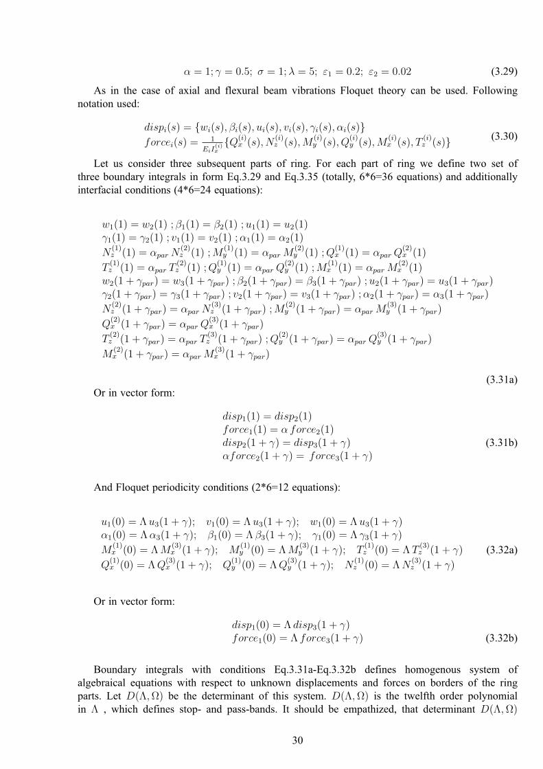
One can plot dependency Λ of Ω, for example from condition 𝐷𝑤,𝑢(Λ,Ω) = 0 . Unlike thecases considered earlier in [8] there exists three pairs (with property Λ1 * Λ2 = 1) of branchesof solutions Λ𝑖(Ω): one pair of exponentially increasing and decreasing branches (this couple isnot shown below, because this couple has significantly higher (and lower) magnitude than othertwo branches) and two pair of branches that defines stop- and pass-bands, it preserves for bothdeterminants 𝐷𝑤,𝑢 and 𝐷𝛾,𝑣. Below dependence 𝐷𝑤,𝑢(Λ,Ω) = 0 is plotted :

Figure 3.11: Floquet zones for 𝐷𝑤,𝑢(Λ,Ω) and different kinds of zones marked with numbers

One can distinct “real” stop band (marked as 1), where wave propagation fully blocked,itslocation is defined by intersection of stop-bands of two branches (overlapping of an orange stopband and a red stop band on the Fig.3.11).In zone 1 only exponential increasing-decreasing standingwaves are presented. "Partial"gap band (marked as 2) its location defined by overlapping pass bandand stop band of different branches (overlapping of a red stop band and an orange pass band andvice versa). In zone 2 appears one propagating wave. And pass band (marked as 3) its locationdefined as overlapping of two pass bands of different branches (an orange pass band and a red passband) in zone 3 two propagating waves are presented. All three zones contains one pair of standingexponential increasing-decreasing standing waves, which is described above and not shown on thepicture.

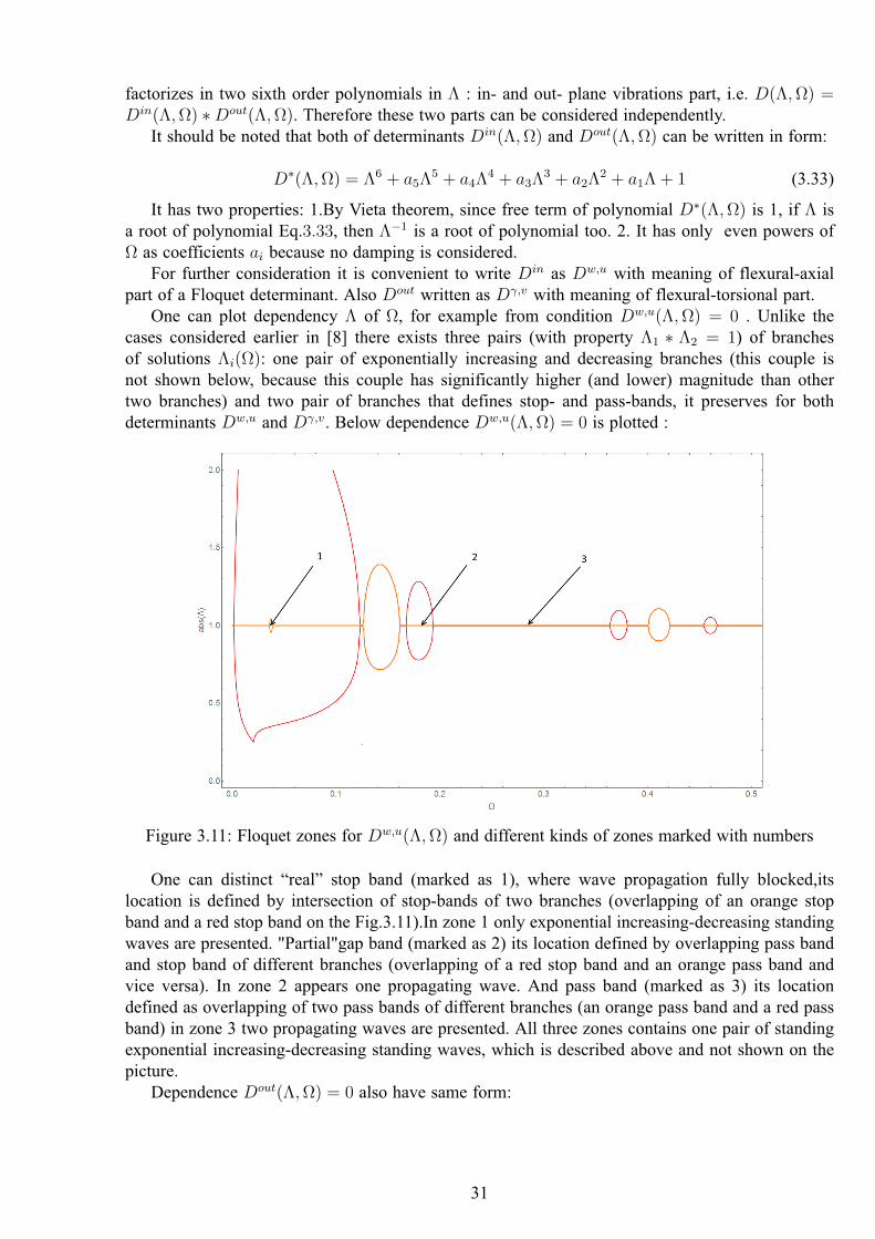
Dependence 𝐷𝑜𝑢𝑡(Λ,Ω) = 0 also have same form:

31

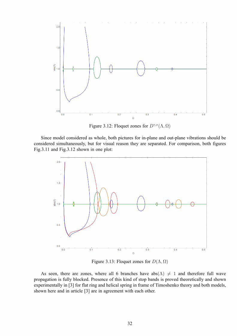
Figure 3.12: Floquet zones for 𝐷𝛾,𝑣(Λ,Ω)

Since model considered as whole, both pictures for in-plane and out-plane vibrations should beconsidered simultaneously, but for visual reason they are separated. For comparison, both figuresFig.3.11 and Fig.3.12 shown in one plot:

Figure 3.13: Floquet zones for 𝐷(Λ,Ω)

As seen, there are zones, where all 6 branches have abs(Λ) = 1 and therefore full wavepropagation is fully blocked. Presence of this kind of stop bands is proved theoretically and shownexperimentally in [3] for flat ring and helical spring in frame of Timoshenko theory and both models,shown here and in article [3] are in agreement with each other.

32

3.3.2 Finite periodic structure

As in previous cases one can introduce concept of a symmetrical periodicity cell shown on theFig.1.3

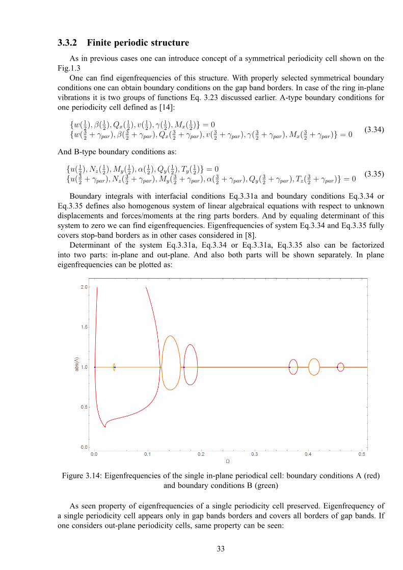
One can find eigenfrequencies of this structure. With properly selected symmetrical boundaryconditions one can obtain boundary conditions on the gap band borders. In case of the ring in-planevibrations it is two groups of functions Eq. 3.23 discussed earlier. A-type boundary conditions forone periodicity cell defined as [14]:

𝑤(12), 𝛽(1

2), 𝑄𝑥(1

2), 𝑣(1

2), 𝛾(1

2),𝑀𝑥(1

2) = 0

𝑤(32

+ 𝛾𝑝𝑎𝑟), 𝛽(32

+ 𝛾𝑝𝑎𝑟), 𝑄𝑥(32

+ 𝛾𝑝𝑎𝑟), 𝑣(32

+ 𝛾𝑝𝑎𝑟), 𝛾(32

+ 𝛾𝑝𝑎𝑟),𝑀𝑥(32

+ 𝛾𝑝𝑎𝑟) = 0(3.34)

And B-type boundary conditions as:

𝑢(12), 𝑁𝑧(

12),𝑀𝑦(

12), 𝛼(1

2), 𝑄𝑦(

12), 𝑇𝑦(

12) = 0

𝑢(32

+ 𝛾𝑝𝑎𝑟), 𝑁𝑧(32

+ 𝛾𝑝𝑎𝑟),𝑀𝑦(32

+ 𝛾𝑝𝑎𝑟), 𝛼(32

+ 𝛾𝑝𝑎𝑟), 𝑄𝑦(32

+ 𝛾𝑝𝑎𝑟), 𝑇𝑧(32

+ 𝛾𝑝𝑎𝑟) = 0(3.35)

Boundary integrals with interfacial conditions Eq.3.31a and boundary conditions Eq.3.34 orEq.3.35 defines also homogenous system of linear algebraical equations with respect to unknowndisplacements and forces/moments at the ring parts borders. And by equaling determinant of thissystem to zero we can find eigenfrequencies. Eigenfrequencies of system Eq.3.34 and Eq.3.35 fullycovers stop-band borders as in other cases considered in [8].

Determinant of the system Eq.3.31a, Eq.3.34 or Eq.3.31a, Eq.3.35 also can be factorizedinto two parts: in-plane and out-plane. And also both parts will be shown separately. In planeeigenfrequencies can be plotted as:

Figure 3.14: Eigenfrequencies of the single in-plane periodical cell: boundary conditions A (red)and boundary conditions B (green)

As seen property of eigenfrequencies of a single periodicity cell preserved. Eigenfrequency ofa single periodicity cell appears only in gap bands borders and covers all borders of gap bands. Ifone considers out-plane periodicity cells, same property can be seen:

33

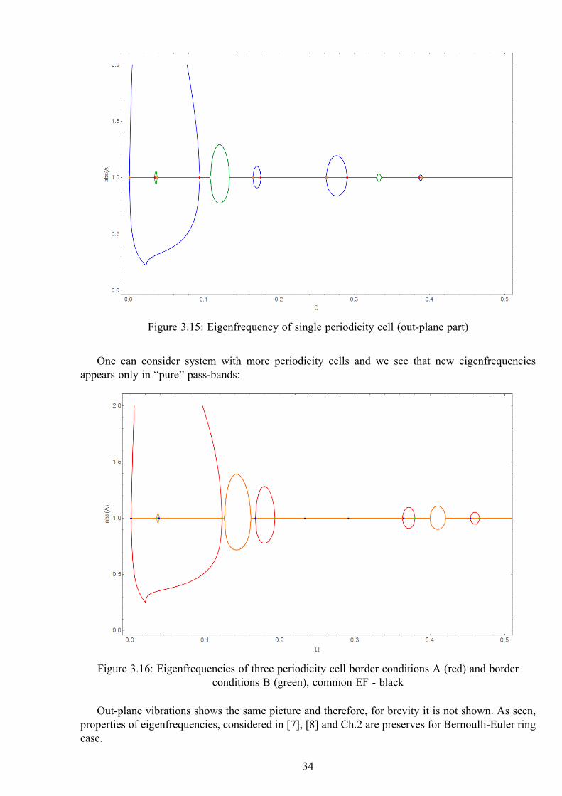
Figure 3.15: Eigenfrequency of single periodicity cell (out-plane part)

One can consider system with more periodicity cells and we see that new eigenfrequenciesappears only in “pure” pass-bands:

Figure 3.16: Eigenfrequencies of three periodicity cell border conditions A (red) and borderconditions B (green), common EF - black

Out-plane vibrations shows the same picture and therefore, for brevity it is not shown. As seen,properties of eigenfrequencies, considered in [7], [8] and Ch.2 are preserves for Bernoulli-Euler ringcase.

34

3.3.3 Eigenmodes analysis

Eingenmode analysis gives clear understanding of wave propagation picture in infinitewaveguide. Form of waves and energy transmission mode (standing or propagating wave) canbe easily shown when eigenmodes analysis is performed. Also it is first step to strain state analysis,which is often of interest in engineering practice.

First same procedure used and determinant 𝐷(Λ,Ω) obtained from system Eq.3.31a-Eq.3.32b.As shown above in case of a flat ring second branch of Floquet zones appears. And differencebetween full and partial gap-band can be considered (see Fig.3.12).

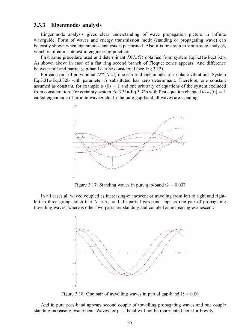
For each root of polynomial 𝐷𝑖𝑛(Λ,Ω) one can find eigenmodes of in-plane vibrations. SystemEq.3.31a-Eq.3.32b with parameter Λ substituted has zero determinant. Therefore, one constantassumed as constant, for example 𝑢1(0) = 1 and one arbitrary of equations of the system excludedfrom consideration. For certainty system Eq.3.31a-Eq.3.32b with first equation changed to 𝑢1(0) = 1called eigenmode of infinite waveguide. In the pure gap-band all waves are standing:

Figure 3.17: Standing waves in pure gap-band Ω = 0.037

In all cases all waved coupled as increasing-evanescent or traveling from left to right and right-left in three groups such that Λ1 * Λ2 = 1. In partial gap-band appears one pair of propagatingtravelling waves, whereas other two pairs are standing and coupled as increasing-evanescent:

Figure 3.18: One pair of travelling waves in partial gap-band Ω = 0.06

And in pure pass-band appears second couple of travelling propagating waves and one couplestanding increasing-evanescent. Waves for pass-band will not be represented here for brevity.

35

3.4 The spatial periodic structure

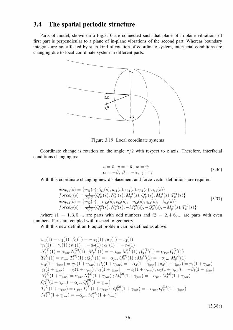
Parts of model, shown on a Fig.3.10 are connected such that plane of in-plane vibrations offirst part is perpendicular to a plane of in-plane vibrations of the second part. Whereas boundaryintegrals are not affected by such kind of rotation of coordinate system, interfacial conditions arechanging due to local coordinate system in different parts:

Figure 3.19: Local coordinate systems

Coordinate change is rotation on the angle 𝜋/2 with respect to z axis. Therefore, interfacialconditions changing as:

𝑢 = 𝑣, 𝑣 = −, 𝑤 = 𝛼 = −𝛽, 𝛽 = −, 𝛾 = 𝛾

(3.36)

With this coordinate changing new displacement and force vector definitions are required

𝑑𝑖𝑠𝑝𝑖1(𝑠) = 𝑤𝑖1(𝑠), 𝛽𝑖1(𝑠), 𝑢𝑖1(𝑠), 𝑣𝑖1(𝑠), 𝛾𝑖1(𝑠), 𝛼𝑖1(𝑠)𝑓𝑜𝑟𝑐𝑒𝑖1(𝑠) = 1

𝐸𝑖𝐼𝑖1𝑥𝑄𝑖1

𝑥 (𝑠), 𝑁 𝑖1𝑧 (𝑠),𝑀 𝑖1

𝑦 (𝑠), 𝑄𝑖1𝑦 (𝑠),𝑀 𝑖1

𝑥 (𝑠), 𝑇 𝑖1𝑧 (𝑠)

𝑑𝑖𝑠𝑝𝑖2(𝑠) = 𝑤𝑖2(𝑠),−𝛼𝑖2(𝑠), 𝑣𝑖2(𝑠),−𝑢𝑖2(𝑠), 𝛾𝑖2(𝑠),−𝛽𝑖2(𝑠)𝑓𝑜𝑟𝑐𝑒𝑖2(𝑠) = 1

𝐸𝑖𝐼𝑖2𝑥𝑄𝑖2

𝑦 (𝑠), 𝑁 𝑖2𝑧 (𝑠),−𝑀 𝑖2

𝑥 (𝑠),−𝑄𝑖2𝑥 (𝑠),−𝑀 𝑖2

𝑦 (𝑠), 𝑇 𝑖2𝑧 (𝑠)

(3.37)

,where 𝑖1 = 1, 3, 5, ... are parts with odd numbers and 𝑖2 = 2, 4, 6, ... are parts with evennumbers. Parts are coupled with respect to geometry.

With this new definition Floquet problem can be defined as above:

𝑤1(1) = 𝑤2(1) ; 𝛽1(1) = −𝛼2(1) ;𝑢1(1) = 𝑣2(1)𝛾1(1) = 𝛾2(1) ; 𝑣1(1) = −𝑢2(1) ;𝛼1(1) = −𝛽2(1)

𝑁(1)𝑧 (1) = 𝛼𝑝𝑎𝑟 𝑁

(2)𝑧 (1) ;𝑀

(1)𝑦 (1) = −𝛼𝑝𝑎𝑟 𝑀

(2)𝑥 (1) ;𝑄

(1)𝑥 (1) = 𝛼𝑝𝑎𝑟 𝑄

(2)𝑦 (1)

𝑇(1)𝑧 (1) = 𝛼𝑝𝑎𝑟 𝑇

(2)𝑧 (1) ;𝑄

(1)𝑦 (1) = −𝛼𝑝𝑎𝑟 𝑄

(2)𝑥 (1) ;𝑀

(1)𝑥 (1) = −𝛼𝑝𝑎𝑟 𝑀

(2)𝑦 (1)

𝑤2(1 + 𝛾𝑝𝑎𝑟) = 𝑤3(1 + 𝛾𝑝𝑎𝑟) ; 𝛽2(1 + 𝛾𝑝𝑎𝑟) = −𝛼3(1 + 𝛾𝑝𝑎𝑟) ;𝑢2(1 + 𝛾𝑝𝑎𝑟) = 𝑣3(1 + 𝛾𝑝𝑎𝑟)𝛾2(1 + 𝛾𝑝𝑎𝑟) = 𝛾3(1 + 𝛾𝑝𝑎𝑟) ; 𝑣2(1 + 𝛾𝑝𝑎𝑟) = −𝑢3(1 + 𝛾𝑝𝑎𝑟) ;𝛼2(1 + 𝛾𝑝𝑎𝑟) = −𝛽3(1 + 𝛾𝑝𝑎𝑟)

𝑁(2)𝑧 (1 + 𝛾𝑝𝑎𝑟) = 𝛼𝑝𝑎𝑟 𝑁

(3)𝑧 (1 + 𝛾𝑝𝑎𝑟) ;𝑀

(2)𝑦 (1 + 𝛾𝑝𝑎𝑟) = −𝛼𝑝𝑎𝑟 𝑀

(3)𝑥 (1 + 𝛾𝑝𝑎𝑟)

𝑄(2)𝑥 (1 + 𝛾𝑝𝑎𝑟) = 𝛼𝑝𝑎𝑟 𝑄

(3)𝑦 (1 + 𝛾𝑝𝑎𝑟)

𝑇(2)𝑧 (1 + 𝛾𝑝𝑎𝑟) = 𝛼𝑝𝑎𝑟 𝑇

(3)𝑧 (1 + 𝛾𝑝𝑎𝑟) ;𝑄

(2)𝑦 (1 + 𝛾𝑝𝑎𝑟) = −𝛼𝑝𝑎𝑟 𝑄

(3)𝑥 (1 + 𝛾𝑝𝑎𝑟)

𝑀(2)𝑥 (1 + 𝛾𝑝𝑎𝑟) = −𝛼𝑝𝑎𝑟 𝑀

(3)𝑦 (1 + 𝛾𝑝𝑎𝑟)

(3.38a)

36

Or in vector form:

𝑑𝑖𝑠𝑝1(1) = 𝑑𝑖𝑠𝑝2(1)𝑓𝑜𝑟𝑐𝑒1(1) = 𝛼 𝑓𝑜𝑟𝑐𝑒2(1)𝑑𝑖𝑠𝑝2(1 + 𝛾) = 𝑑𝑖𝑠𝑝3(1 + 𝛾)𝛼𝑓𝑜𝑟𝑐𝑒2(1 + 𝛾) = 𝑓𝑜𝑟𝑐𝑒3(1 + 𝛾)𝑑𝑖𝑠𝑝1(0) = Λ 𝑑𝑖𝑠𝑝3(1 + 𝛾)𝑓𝑜𝑟𝑐𝑒1(0) = Λ 𝑓𝑜𝑟𝑐𝑒3(1 + 𝛾)

(3.38b)

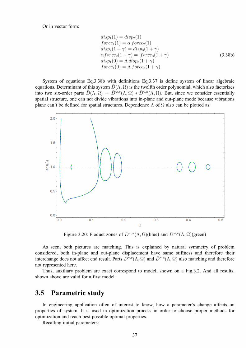
System of equations Eq.3.38b with definitions Eq.3.37 is define system of linear algebraicequations. Determinant of this system (Λ,Ω) is the twelfth order polynomial, which also factorizesinto two six-order parts (Λ,Ω) = 𝑤,𝑣(Λ,Ω) * 𝛾,𝑢(Λ,Ω). But, since we consider essentiallyspatial structure, one can not divide vibrations into in-plane and out-plane mode because vibrationsplane can’t be defined for spatial structures. Dependence Λ of Ω also can be plotted as:

Figure 3.20: Floquet zones of 𝐷𝑤,𝑢(Λ,Ω)(blue) and 𝑤,𝑣(Λ,Ω)(green)

As seen, both pictures are matching. This is explained by natural symmetry of problemconsidered, both in-plane and out-plane displacement have same stiffness and therefore theirinterchange does not affect end result. Parts 𝐷𝛾,𝑣(Λ,Ω) and 𝛾,𝑢(Λ,Ω) also matching and thereforenot represented here.

Thus, auxiliary problem are exact correspond to model, shown on a Fig.3.2. And all results,shown above are valid for a first model.

3.5 Parametric study

In engineering application often of interest to know, how a parameter’s change affects onproperties of system. It is used in optimization process in order to choose proper methods foroptimization and reach best possible optimal properties.

Recalling initial parameters:

37

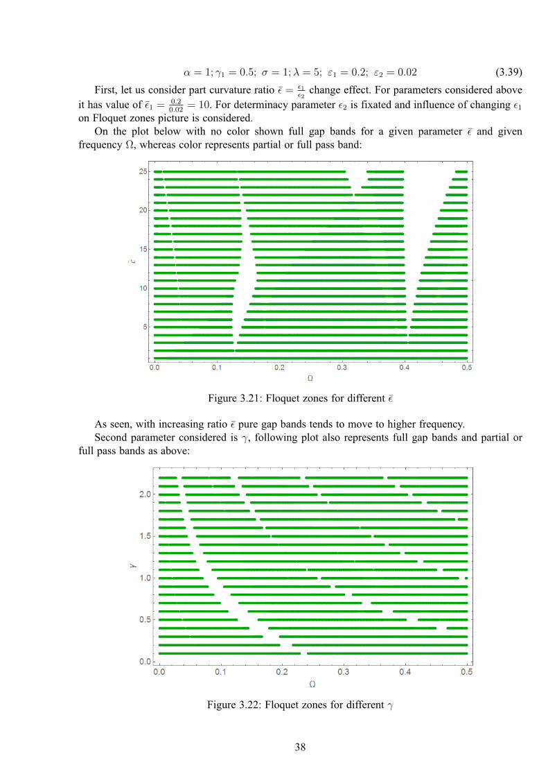
𝛼 = 1; 𝛾1 = 0.5; 𝜎 = 1;𝜆 = 5; 𝜀1 = 0.2; 𝜀2 = 0.02 (3.39)

First, let us consider part curvature ratio 𝜖 = 𝜖1𝜖2

change effect. For parameters considered aboveit has value of 𝜖1 = 0.2

0.02= 10. For determinacy parameter 𝜖2 is fixated and influence of changing 𝜖1

on Floquet zones picture is considered.On the plot below with no color shown full gap bands for a given parameter 𝜖 and given

frequency Ω, whereas color represents partial or full pass band:

Figure 3.21: Floquet zones for different 𝜖

As seen, with increasing ratio 𝜖 pure gap bands tends to move to higher frequency.Second parameter considered is 𝛾, following plot also represents full gap bands and partial or

full pass bands as above:

Figure 3.22: Floquet zones for different 𝛾

38

For 𝛾 we have reciprocal tendency, with increasing 𝛾 gap bands tends to move to lowerfrequency.

This parameter study in showing that model considered can be used for engineering applicationsfor optimization processes and obtaining properties, demanded by the industry and considering basicideas of influence of parameters on pure gap band positions.

In this chapter first model of a torque vibration isolator was considered. It has been modelledas a system of differential equations for an infinite periodic structure. Therefore, methods, used inCh.2, were expanded to a system of a differential equation. Green’s matrix coefficient with usingbi-orthogonality condition were obtained in analytical form. Difference between Floquet zones ofa single differential equation and system of differential equation was shown. Also, was shownindependence with respect to symmetry transformation of Floquet zones for a structure with naturalsymmetry. Also parameters study was conducted in order to show one of industrial applications ofgiven model.

39

Conclusion and future work

First part of this master project has two main goals: theoretical and practical. In practical point ofview torque simple vibration isolator model was considered and vibration isolation properties of thisstructure were considered. Model shows that full waves propagation block can be reached in lowfrequency region, that of interest in industrial applications. Also, possibility of model optimizationwas shown, but deep investigation of optimization of properties are out of scope of this project.

From theoretical point of view, all main principles of Floquet theory have been developed andshown on examples. Possibility of using of polar coordinates were considered. Also first step inhierarchy of torque vibration isolator models were considered. Model of torque vibration isolatorhas been developed and considered in frame of Floquet zones theory. Tools that developed in thispart of master’s project have broad range of applicability and they will be used in second part ofwork. Results obtained in this part will be used for comparison with second model, which will beconsidered in second part of master’s project.

One of supplementary goals was to develop and validate the program that can be used formodelling of an isolator. Wolfram Mathematica software was used for programming, because it fitsbest for analytical modelling.

Also, first parts gives all necessary theory, shown in examples and with all necessary references,that allows one to use differential equations in modelling of vibrations of physical structures.

Goal reached in this part, gives following propositions for goals of second part:(I) Consider second model circular plate-cylindrical shell, using developed for polar coordinate

system Floquet theory from theoretical and practical point of view(II) Compare first and second model in order to consider advantages and disadvantages of choice

of more complicated model. Also it is of interest in theoretical point of view to compare Floquettheory for different coordinate system.

(III)Conduct experiments in order to validate models and developed theory and define practicalapplicability of considered in both parts of masters’s project models

Both parts allows one to build hierarchy of two models of torque vibration isolator, that useswide range of methods with wide range of applicability.

40

Literature

1. L.Brillouin. Wave Propagation in Periodic Structures second ed. Dover Publications New York,1953.

2. D.J.Mead. Wave propagation in continuous periodic structures. Research contributions fromSouthampton 1964-1995 // Journal of Sound and Vibration. 1996. Vol. 190. P. 495–524.

3. A.Søe-Knudsen, R.Darula, Sorokin S. Theoretical and experimental analysis of the stop-bandbehavior of elastic springs with periodically discontinuous of curvature // Journal of the Acous-tical Society of America. 2012. Vol. 132. P. 1378–1383.

4. A.Søe-Knudsen, Sorokin S. Modelling of linear wave propagation in spatial fluid filled pipesystems consisting of elastic curved and straight elements // Journal of Sound and Vibration.2010. Vol. 329. P. 5116–5146.

5. A.Søe-Knudsen. Design of stop-band filter by use of curved pipe segments and shape optimiza-tion // Structural and Multidisciplinary Optimization. 2011. Vol. 44. P. 863–874.

6. A.Søe-Knudsen. Design of stop-band filters by use of compound curved pipe segmentsand shape optimization // 10th International Conference on Recent Advances in StructuralDynamics. Institute of Sound and Vibration Research, 2010.

7. A.Hvatov, S.Sorokin. Analysis of eigenfrequencies of finite periodic structures in view of loca-tion of frequency pas- and stop-bands // Proceedings of 20th International Congress on Soundand Vibration. 2013.

8. A.Hvatov, S.Sorokin. Free vibrations of finite periodic structures in pass- and stop-bands of thecounterpart infinite waveguides // Journal of Sound and Vibration. 2015. Vol. 347. P. 200–217.

9. S.Sorokin. On the bi-orthogonality conditions for multi-modal elastic waveguides. // Journal ofSound and Vibration. 2013. Vol. 332. P. 5606–5617.

10. Dym C. L., I.H.Shames. Solid Mechanics. A Variational Approach, Augmented Edition.Springer, 2013.

11. Duffy D. G. Green’s Functions with Applications. Chapman and Hall, 2001.

12. Skudrzyk E. The Foundations of Acoustics. Basic mathematics and basic acoustics. Springer-Verlag, 1971.

13. Achenbach J. D. Reciprocity in Elastodynamics. Cambridge University Press, 2003.

14. S.Sorokin. The Green’s matrix and the boundary integral equations for analysis of time-harmonic dynamics of elastic helical springs. // Journal of the Acoustical Society of America.2011. Vol. 129. P. 1315–1323.

15. R.Nielsen, S.Sorokin. Periodicity effects of axial waves in elastic compound rods // Journal ofSound and Vibration. 2015. Vol. 353. P. 135–149.

41

Appendix A

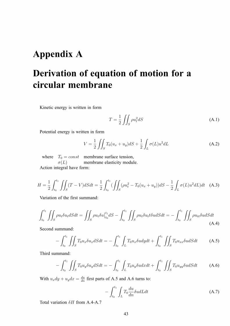
Derivation of equation of motion for acircular membrane

Kinetic energy is written in form

𝑇 =1

2

∫∫𝑆

𝜌𝑢2𝑡𝑑𝑆 (A.1)

Potential energy is written in form

𝑉 =1

2

∫∫𝑆

𝑇0(𝑢𝑥 + 𝑢𝑦)𝑑𝑆 +1

2

∫𝐿

𝜎(𝐿)𝑢2𝑑𝐿 (A.2)

where 𝑇0 = 𝑐𝑜𝑛𝑠𝑡 membrane surface tension,𝜎(𝐿) membrane elasticity module.

Action integral have form:

𝐻 =1

2

∫ 𝑡1

𝑡0

∫∫𝑆

(𝑇 − 𝑉 )𝑑𝑆𝑑𝑡 =1

2

∫ 𝑡1

𝑡0

(

∫∫𝑆

(𝜌𝑢2𝑡 − 𝑇0(𝑢𝑥 + 𝑢𝑦))𝑑𝑆 − 1

2

∫𝐿

𝜎(𝐿)𝑢2𝑑𝐿)𝑑𝑡 (A.3)

Variation of the first summand:

∫ 𝑡1

𝑡0

∫∫𝑆

𝜌𝑢𝑡𝛿𝑢𝑡𝑑𝑆𝑑𝑡 =

∫∫𝑆

𝜌𝑢𝑡𝛿𝑢𝑡1𝑡0𝑑𝑆 −

∫ 𝑡1

𝑡0

∫∫𝑆

𝜌𝑢𝑡𝛿𝑢𝑡𝑡𝛿𝑢𝑑𝑆𝑑𝑡 = −∫ 𝑡1

𝑡0

∫∫𝑆

𝜌𝑢𝑡𝑡𝛿𝑢𝑑𝑆𝑑𝑡

(A.4)Second summand:

−∫ 𝑡1

𝑡0

∫∫𝑆

𝑇0𝑢𝑥𝛿𝑢𝑥𝑑𝑆𝑑𝑡 = −∫ 𝑡1

𝑡0

∫𝐿

𝑇0𝑢𝑥𝛿𝑢𝑑𝑦𝑑𝑡 +

∫ 𝑡1

𝑡0

∫∫𝑆

𝑇0𝑢𝑥𝑥𝛿𝑢𝑑𝑆𝑑𝑡 (A.5)

Third summand:

−∫ 𝑡1

𝑡0

∫∫𝑆

𝑇0𝑢𝑦𝛿𝑢𝑦𝑑𝑆𝑑𝑡 = −∫ 𝑡1

𝑡0

∫𝐿

𝑇0𝑢𝑦𝛿𝑢𝑑𝑥𝑑𝑡 +

∫ 𝑡1

𝑡0

∫∫𝑆

𝑇0𝑢𝑦𝑦𝛿𝑢𝑑𝑆𝑑𝑡 (A.6)

With 𝑢𝑥𝑑𝑦 + 𝑢𝑦𝑑𝑥 = 𝑑𝑢𝑑𝑛

first parts of A.5 and A.6 turns to:

−∫ 𝑡1

𝑡0

∫𝐿

𝑇0𝑑𝑢

𝑑𝑛𝛿𝑢𝑑𝐿𝑑𝑡 (A.7)

Total variation 𝛿𝐻 from A.4-A.7

43

𝛿𝐻 =

∫ 𝑡1

𝑡0

∫𝐿

(𝜎(𝐿)𝑢− 𝑇0𝑑𝑢

𝑑𝑛)𝛿𝑢𝑑𝐿𝑑𝑡 +

∫ 𝑡1

𝑡0

∫∫𝑆

(𝑇0(𝑢𝑥𝑥 + 𝑢𝑦𝑦) − 𝜌𝑢𝑡𝑡)𝛿𝑢𝑑𝑆𝑑𝑡 (A.8)

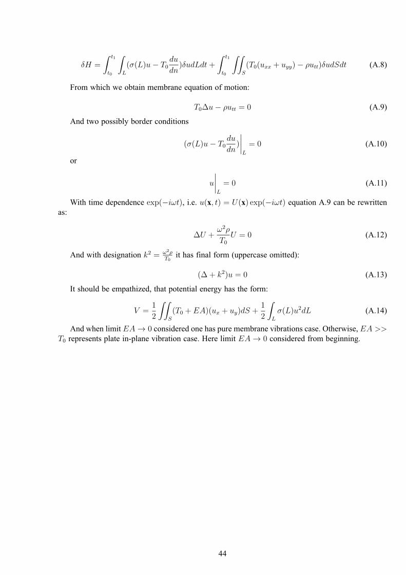
From which we obtain membrane equation of motion:

𝑇0∆𝑢− 𝜌𝑢𝑡𝑡 = 0 (A.9)

And two possibly border conditions

(𝜎(𝐿)𝑢− 𝑇0𝑑𝑢

𝑑𝑛)

𝐿

= 0 (A.10)

or

𝑢

𝐿

= 0 (A.11)

With time dependence exp(−𝑖𝜔𝑡), i.e. 𝑢(x, 𝑡) = 𝑈(x) exp(−𝑖𝜔𝑡) equation A.9 can be rewrittenas:

∆𝑈 +𝜔2𝜌

𝑇0

𝑈 = 0 (A.12)

And with designation 𝑘2 = 𝜔2𝜌𝑇0

it has final form (uppercase omitted):

(∆ + 𝑘2)𝑢 = 0 (A.13)

It should be empathized, that potential energy has the form:

𝑉 =1

2

∫∫𝑆

(𝑇0 + 𝐸𝐴)(𝑢𝑥 + 𝑢𝑦)𝑑𝑆 +1

2

∫𝐿

𝜎(𝐿)𝑢2𝑑𝐿 (A.14)

And when limit 𝐸𝐴 → 0 considered one has pure membrane vibrations case. Otherwise, 𝐸𝐴 >>𝑇0 represents plate in-plane vibration case. Here limit 𝐸𝐴 → 0 considered from beginning.

44

Appendix B

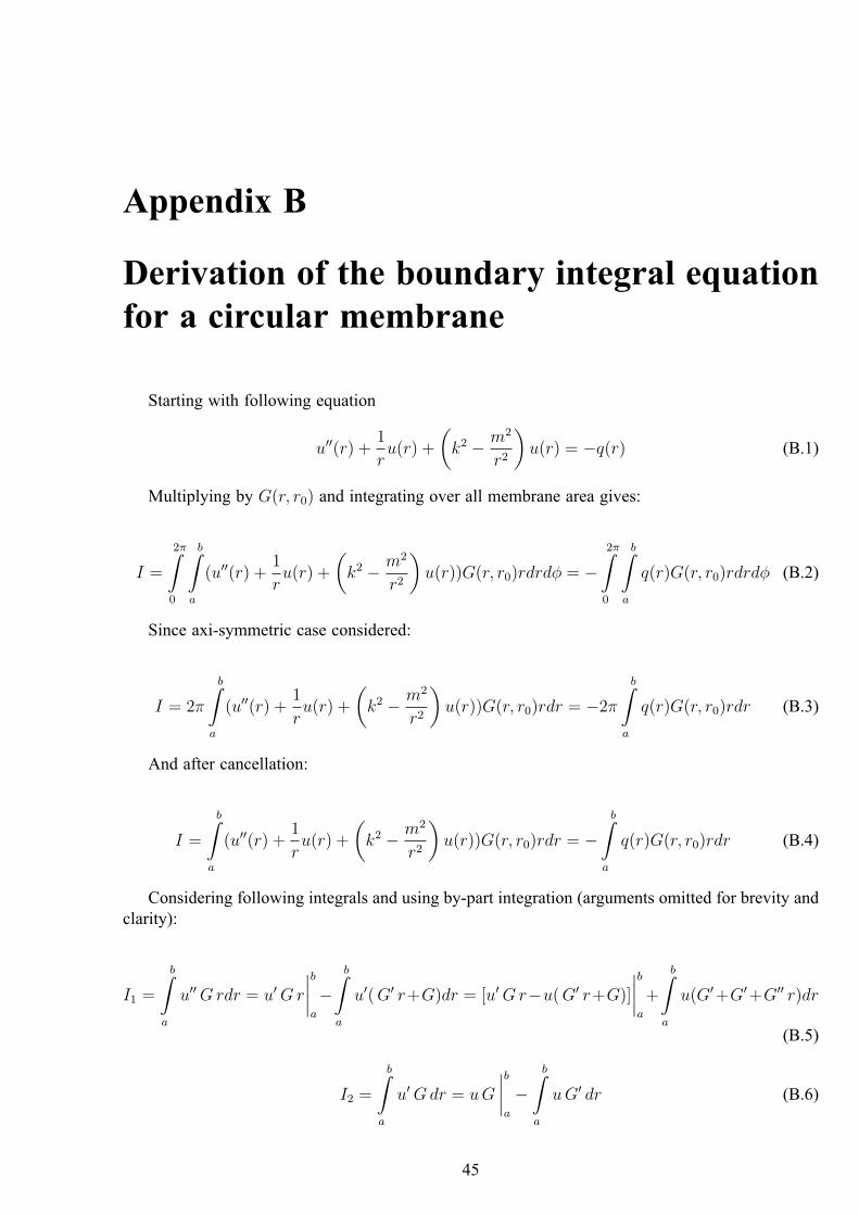
Derivation of the boundary integral equationfor a circular membrane

Starting with following equation

𝑢′′(𝑟) +1

𝑟𝑢(𝑟) +

(𝑘2 − 𝑚2

𝑟2

)𝑢(𝑟) = −𝑞(𝑟) (B.1)

Multiplying by 𝐺(𝑟, 𝑟0) and integrating over all membrane area gives:

𝐼 =

2𝜋∫0

𝑏∫𝑎

(𝑢′′(𝑟) +1

𝑟𝑢(𝑟) +

(𝑘2 − 𝑚2

𝑟2

)𝑢(𝑟))𝐺(𝑟, 𝑟0)𝑟𝑑𝑟𝑑𝜑 = −

2𝜋∫0

𝑏∫𝑎

𝑞(𝑟)𝐺(𝑟, 𝑟0)𝑟𝑑𝑟𝑑𝜑 (B.2)

Since axi-symmetric case considered:

𝐼 = 2𝜋

𝑏∫𝑎

(𝑢′′(𝑟) +1

𝑟𝑢(𝑟) +

(𝑘2 − 𝑚2

𝑟2

)𝑢(𝑟))𝐺(𝑟, 𝑟0)𝑟𝑑𝑟 = −2𝜋

𝑏∫𝑎

𝑞(𝑟)𝐺(𝑟, 𝑟0)𝑟𝑑𝑟 (B.3)

And after cancellation:

𝐼 =

𝑏∫𝑎

(𝑢′′(𝑟) +1

𝑟𝑢(𝑟) +

(𝑘2 − 𝑚2

𝑟2

)𝑢(𝑟))𝐺(𝑟, 𝑟0)𝑟𝑑𝑟 = −

𝑏∫𝑎

𝑞(𝑟)𝐺(𝑟, 𝑟0)𝑟𝑑𝑟 (B.4)

Considering following integrals and using by-part integration (arguments omitted for brevity andclarity):

𝐼1 =

𝑏∫𝑎

𝑢′′ 𝐺𝑟𝑑𝑟 = 𝑢′ 𝐺𝑟

𝑏𝑎

−𝑏∫

𝑎

𝑢′(𝐺′ 𝑟+𝐺)𝑑𝑟 = [𝑢′ 𝐺𝑟−𝑢(𝐺′ 𝑟+𝐺)]

𝑏𝑎

+

𝑏∫𝑎

𝑢(𝐺′+𝐺′+𝐺′′ 𝑟)𝑑𝑟

(B.5)

𝐼2 =

𝑏∫𝑎

𝑢′ 𝐺𝑑𝑟 = 𝑢𝐺

𝑏𝑎

−𝑏∫

𝑎

𝑢𝐺′ 𝑑𝑟 (B.6)

45

𝐼3 =

𝑏∫𝑎

(𝑘2 − 𝑚2

𝑟2

)𝑢𝐺 𝑟𝑑𝑟 (B.7)

Substituting B.5-B.7 into B.4 gives:

𝐼 = 𝐼1 + 𝐼2 + 𝐼3 = [𝑢′ 𝐺𝑟 − 𝑢𝐺′ 𝑟]

𝑏𝑎

+

𝑏∫𝑎

(𝐺′′ +1

𝑟𝐺′ +

(𝑘2 − 𝑚2

𝑟2

)𝐺)𝑢 𝑟𝑑𝑟 (B.8)

Recalling modified Green’s function definition:

𝐺′′(𝑟, 𝑟0) +1

𝑟𝐺′(𝑟, 𝑟0) +

(𝑘2 − 𝑚2

𝑟2

)𝐺(𝑟, 𝑟0) = −𝛿(𝑟 − 𝑟0)

𝑟0(B.9)

With definition B.9 equation B.8 has the form:

𝐼 = [𝑢′(𝑟)𝐺(𝑟, 𝑟0) − 𝑢(𝑟)𝐺′(𝑟, 𝑟0)]𝑟

𝑟=𝑏

𝑟=𝑎

+

𝑏∫𝑎

−𝛿(𝑟 − 𝑟0)

𝑟0𝑢(𝑟) 𝑟𝑑𝑟 (B.10)

And with property of delta function it can be rewritten as:

𝐼 = [𝑢′(𝑟)𝐺(𝑟, 𝑟0) − 𝑢(𝑟)𝐺′(𝑟, 𝑟0)]𝑟

𝑟=𝑏

𝑟=𝑎

− 𝑢(𝑟0) 𝑟0𝑟0

(B.11)

Here modified Green’s function used, in term 𝑢(𝑟0) 𝑟0𝑟0

cancelled 𝑟0 and boundary equation hasmore simple form.Also, it can be rewritten with recalled right hand side of B.4 in form:

𝑢(𝑟0) = [𝑢′(𝑟)𝐺(𝑟, 𝑟0) − 𝑢(𝑟)𝐺′(𝑟, 𝑟0)]𝑟

𝑟=𝑏

𝑟=𝑎

+

𝑏∫𝑎

𝑞(𝑟)𝐺(𝑟, 𝑟0)𝑑𝑟 (B.12)

46

Appendix C

Axial rod vibrations in boundary equationsmethod point of view

C.1 Green’s function definition and derivation

Axial beam vibration can be described with following equation:

𝑢𝑥𝑥 −1

𝑐2𝑢𝑡𝑡 = −𝑞(𝑥, 𝑡) (C.1)

,where 𝑐 has meaning of sound of speed (speed of elastic wave propagation) and q(x,t) is theforce density.

With harmonic vibrations state assumed 𝑢(𝑥, 𝑡) = exp[(−𝑖𝜔𝑡)𝑈(𝑥) Eq.C.1 can be rewritten as:

𝑢′′(𝑥) + 𝑘2𝑢(𝑥) = −𝑞(𝑥) (C.2)

,where 𝑘 = 𝜔𝑐

called wave number. In what follows harmonic vibrations state assumed anduppercase of letters is omited.

Green’s function by definition is a solution of the equation with force density 𝑞(𝑥) = 𝛿(𝑥− 𝑥0),where 𝛿(𝑥) is Dirac’s delta function. In the rod axial vibrations case it has meaning of a point forceacting at point 𝑥 with observation point 𝑥0 and Green’s function equation can be written as:

𝑑2

𝑑𝑥2𝐺(𝑥, 𝑥0) + 𝑘2𝐺(𝑥, 𝑥0) = −𝛿(𝑥− 𝑥0) (C.3)

It can be proven that Green’s function should satisfy following properties:

𝐺(𝑥, 𝑥0) = 𝐺(𝑥0, 𝑥)𝜕𝜕𝑥𝐺(𝑥0, 𝑥0 + 𝜀) − 𝜕

𝜕𝑥𝐺(𝑥0, 𝑥0 − 𝜀) = −1, 𝜀 → 0

𝐺(𝑥0, 𝑥0 + 𝜀) = 𝐺(𝑥0, 𝑥0 − 𝜀), 𝜀 → 0(C.4)

Since common solution of homogenous equation C.2 has the form:

𝑢(𝑥) = 𝐶1 exp(𝑖𝑘𝑥) + 𝐶2 exp(−𝑖𝑘𝑥) (C.5)

Solution of equation can be written in form (if one should consider infinite beam it is veryimportant that function 𝐺(𝑥, 𝑥0) should satisfy radiation conditions at infinity [12]):

𝐺+(𝑥, 𝑥0) = 𝐴 exp(𝑖𝑘𝑥) , 𝑥 > 𝑥0

𝐺−(𝑥, 𝑥0) = 𝐵 exp(−𝑖𝑘𝑥) , 𝑥 ≤ 𝑥0(C.6)

Green’s function in form Eq.C.6 substituted into two last properties in C.4 gives:

47

𝐺+(𝑥0, 𝑥0) = 𝐺−(𝑥0, 𝑥0)

𝑑𝑑𝑥

(𝐺+(𝑥, 𝑥0) −𝐺−(𝑥, 𝑥0))

𝑥=𝑥0

= −1(C.7)

or in explicit form:

𝐴 exp(𝑖𝑘𝑥0) = 𝐵 exp(−𝑖𝑘𝑥0)𝑖𝑘𝐴 exp(𝑖𝑘𝑥0) + 𝑖𝑘𝐵 exp(−𝑖𝑘𝑥0) = −1

(C7’)

System Eq.C7’ has the unique solution for unknown coefficients 𝐴 and 𝐵:

𝐴,𝐵 = 𝑖

2𝑘exp(−𝑖𝑘𝑥0),

𝑖

2𝑘exp(𝑖𝑘𝑥0) (C.8)

And finally Green’s function can be written as:

𝐺(𝑥, 𝑥0) =

𝑖2𝑘

exp(−𝑖𝑘(𝑥− 𝑥0)) 𝑥 ≤ 𝑥0

𝑖2𝑘

exp(𝑖𝑘(𝑥− 𝑥0)) 𝑥 > 𝑥0

(C.9)

Or in short form:

𝐺(𝑥, 𝑥0) =𝑖

2𝑘exp(𝑖𝑘 abs(𝑥− 𝑥0)) (C.10)

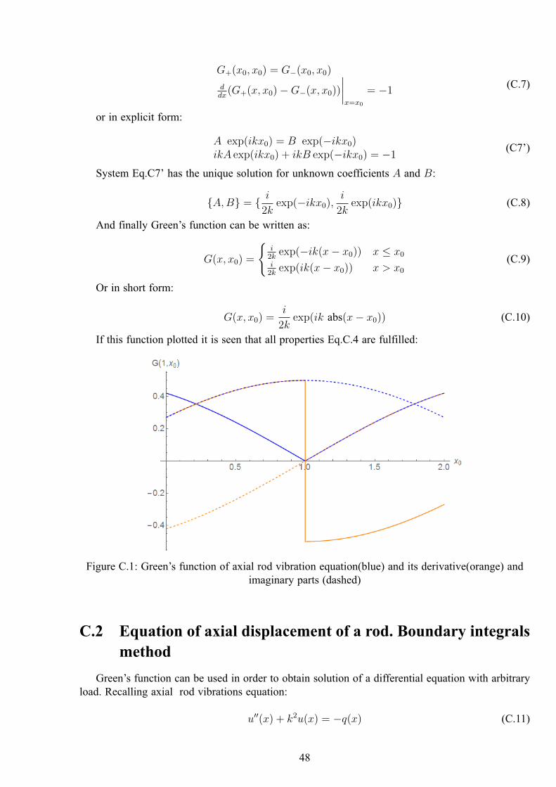
If this function plotted it is seen that all properties Eq.C.4 are fulfilled:

Figure C.1: Green’s function of axial rod vibration equation(blue) and its derivative(orange) andimaginary parts (dashed)

C.2 Equation of axial displacement of a rod. Boundary integralsmethod

Green’s function can be used in order to obtain solution of a differential equation with arbitraryload. Recalling axial rod vibrations equation:

𝑢′′(𝑥) + 𝑘2𝑢(𝑥) = −𝑞(𝑥) (C.11)

48

And Green’s function definition:

𝑑2

𝑑𝑥2𝐺(𝑥, 𝑥0) + 𝑘2𝐺(𝑥, 𝑥0) = −𝛿(𝑥− 𝑥0) (C.12)

In what follows 𝑑𝑑𝑥𝐺(𝑥, 𝑥0) = 𝐺′(𝑥, 𝑥0)

Multiplying equation C.11 on 𝐺(𝑥, 𝑥0) and integrating over beam length

𝑏∫𝑎

(𝑢′′(𝑥) + 𝑘2𝑢(𝑥))𝐺(𝑥, 𝑥0)𝑑𝑥 = −𝑏∫

𝑎

𝑞(𝑥)𝐺(𝑥, 𝑥0)𝑑𝑥 (C.13)

First left hand side of an equation C.13 considered:

𝐼 =

𝑏∫𝑎

(𝑢′′(𝑥) + 𝑘2𝑢(𝑥))𝐺(𝑥, 𝑥0)𝑑𝑥 (C.14)

Considering following integral and using by-part integration:

𝐼1 =𝑏∫𝑎

𝑢′′(𝑥)𝐺(𝑥, 𝑥0)𝑑𝑥 = 𝑢′(𝑥)𝐺(𝑥, 𝑥0) −𝑏∫𝑎

𝑢′(𝑥)𝐺′(𝑥, 𝑥0)𝑑𝑥 =

= [𝑢′(𝑥)𝐺(𝑥, 𝑥0) − 𝑢(𝑥)𝐺′(𝑥, 𝑥0)]

𝑏𝑎

+𝑏∫𝑎

𝑢(𝑥)𝐺′′(𝑥, 𝑥0)𝑑𝑥

(C.15)

And second part of integral just rewritten as:

𝐼2 =

𝑏∫𝑎

𝑘2𝑢(𝑥)𝐺(𝑥, 𝑥0)𝑑𝑥 (C.16)

With using equality 𝐼 = 𝐼1 + 𝐼2 Eq.C.14 can be rewritten:

𝐼 = [𝑢′(𝑥)𝐺(𝑥, 𝑥0) − 𝑢(𝑥)𝐺′(𝑥, 𝑥0)]

𝑏𝑎

+

𝑏∫𝑎

(𝐺′′(𝑥, 𝑥0) + 𝑘2𝐺(𝑥, 𝑥0))𝑢(𝑥)𝑑𝑥 (C.17)

With Green’s function definition Eq.C.12 one can rewrite equation C.17 in form:

𝐼 = [𝑢′(𝑥)𝐺(𝑥, 𝑥0) − 𝑢(𝑥)𝐺′(𝑥, 𝑥0)]

𝑏𝑎

−𝑏∫

𝑎

𝛿(𝑥− 𝑥0)𝑢(𝑥)𝑑𝑥 (C.18)

Dirac’s delta-function has a property:

𝑏∫𝑎

𝑓(𝑥)𝛿(𝑥− 𝑥0)𝑑𝑥 = 𝑓(𝑥0) (C.19)

,which is valid for any range (𝑎, 𝑏) that contains 𝑥0 including (−∞,+∞).With property C.19 and recalling right hand side of C.13 one can rewrite C.18

𝑢(𝑥0) = [𝑢′(𝑥)𝐺(𝑥, 𝑥0) − 𝑢(𝑥)𝐺′(𝑥, 𝑥0)]

𝑏𝑎

+

𝑏∫𝑎

𝑞(𝑥)𝐺(𝑥, 𝑥0)𝑑𝑥 (C.20)

Therefore, if values on a beam boundary are known, one can find displacement at any pointwithin the boundary. Eq.C.20 is called boundary integral equation for an axial rod vibrations.

49

C.3 Boundary integrals method direct application

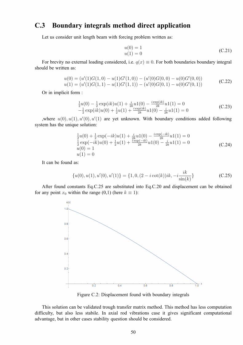
Let us consider unit length beam with forcing problem written as:

𝑢(0) = 1𝑢(1) = 0

(C.21)

For brevity no external loading considered, i.e. 𝑞(𝑥) ≡ 0. For both boundaries boundary integralshould be written as:

𝑢(0) = (𝑢′(1)𝐺(1, 0) − 𝑢(1)𝐺′(1, 0)) − (𝑢′(0)𝐺(0, 0) − 𝑢(0)𝐺′(0, 0))𝑢(1) = (𝑢′(1)𝐺(1, 1) − 𝑢(1)𝐺′(1, 1)) − (𝑢′(0)𝐺(0, 1) − 𝑢(0)𝐺′(0, 1))

(C.22)

Or in implicit form :

12𝑢(0) − 1

2exp(𝑖𝑘)𝑢(1) + 𝑖

2𝑘𝑢1(0) − 𝑖 exp(𝑖𝑘)

2𝑘𝑢1(1) = 0

−12

exp(𝑖𝑘)𝑢(0) + 12𝑢(1) + 𝑖 exp(𝑖𝑘)

2𝑘𝑢1(0) − 𝑖

2𝑘𝑢1(1) = 0

(C.23)

,where 𝑢(0), 𝑢(1), 𝑢′(0), 𝑢′(1) are yet unknown. With boundary conditions added followingsystem has the unique solution:

12𝑢(0) + 1

2exp(−𝑖𝑘)𝑢(1) + 𝑖

2𝑘𝑢1(0) − 𝑖 exp(−𝑖𝑘)

2𝑘𝑢1(1) = 0

12

exp(−𝑖𝑘)𝑢(0) + 12𝑢(1) + 𝑖 exp(−𝑖𝑘)

2𝑘𝑢1(0) − 𝑖

2𝑘𝑢1(1) = 0

𝑢(0) = 1𝑢(1) = 0

(C.24)

It can be found as:

𝑢(0), 𝑢(1), 𝑢′(0), 𝑢′(1) = 1, 0, (2 − 𝑖 cot(𝑘))𝑖𝑘,−𝑖𝑖𝑘

sin(𝑘) (C.25)

After found constants Eq.C.25 are substituted into Eq.C.20 and displacement can be obtainedfor any point 𝑥0 within the range (0,1) (here 𝑘 ≡ 1):

Figure C.2: Displacement found with boundary integrals

This solution can be validated trough transfer matrix method. This method has less computationdifficulty, but also less stabile. In axial rod vibrations case it gives significant computationaladvantage, but in other cases stability question should be considered.

50

Recalling axial rod vibration equation (here also 𝑞(𝑥) ≡ 0):

𝑢′′(𝑥) + 𝑘2𝑢(𝑥) = 0 (C.26)

It has common solution in form:

𝑢(𝑥) = 𝐶1 exp(𝑖𝑘𝑥) + 𝐶2 exp(−𝑖𝑘𝑥) (C.27)

And considering same boundary problem Eq.C.23 one can write following system:

𝑢(0) = 𝐶1 + 𝐶2 = 1𝑢(1) = 𝐶1 exp(𝑖𝑘) + 𝐶2 exp(−𝑖𝑘) = 0

(C.28)

System Eq.C.28 can be solved with respect to unknown integration constaints 𝐶1, 𝐶2 as:

𝐶1, 𝐶2 = 1

1 − exp(2𝑖),

1

1 − exp(−2𝑖) (C.29)

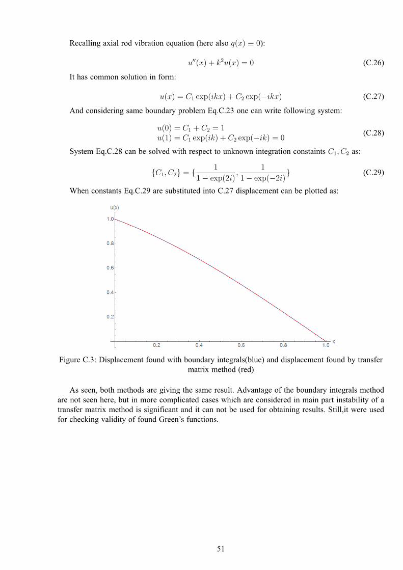
When constants Eq.C.29 are substituted into C.27 displacement can be plotted as:

Figure C.3: Displacement found with boundary integrals(blue) and displacement found by transfermatrix method (red)

As seen, both methods are giving the same result. Advantage of the boundary integrals methodare not seen here, but in more complicated cases which are considered in main part instability of atransfer matrix method is significant and it can not be used for obtaining results. Still,it were usedfor checking validity of found Green’s functions.

51

Appendix D

Floquet theorem. Infinite periodic rod.

Floquet theorem is a very powerful tool for finding solution for a differential equations on ainfinite periodic structures. This is very common theorem for a periodic differential operator andlies out of scope of this work. Nevertheless, it will be shown here for a particular case. Here aninfinite periodic rod axial vibrations case will be considered. Results of this chapter is used in Ch.1for comparison

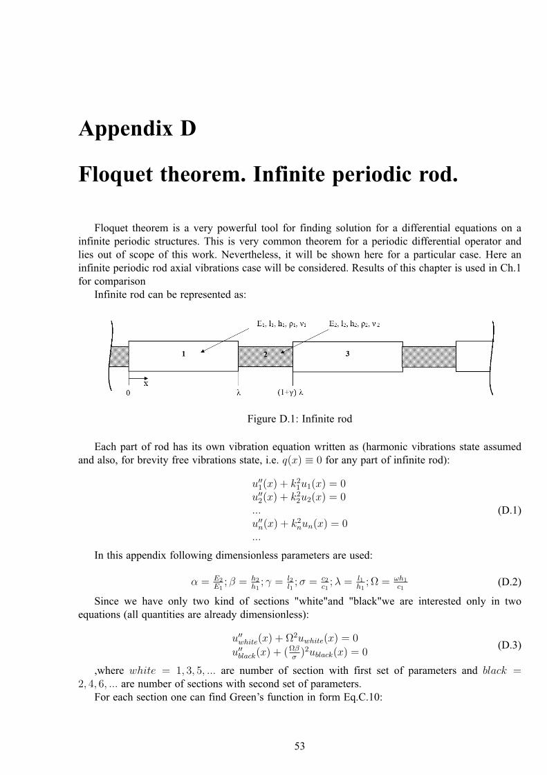
Infinite rod can be represented as:

Figure D.1: Infinite rod

Each part of rod has its own vibration equation written as (harmonic vibrations state assumedand also, for brevity free vibrations state, i.e. 𝑞(𝑥) ≡ 0 for any part of infinite rod):

𝑢′′1(𝑥) + 𝑘2

1𝑢1(𝑥) = 0𝑢′′2(𝑥) + 𝑘2

2𝑢2(𝑥) = 0...𝑢′′𝑛(𝑥) + 𝑘2

𝑛𝑢𝑛(𝑥) = 0...

(D.1)

In this appendix following dimensionless parameters are used:

𝛼 = 𝐸2

𝐸1; 𝛽 = ℎ2

ℎ1; 𝛾 = 𝑙2

𝑙1;𝜎 = 𝑐2

𝑐1;𝜆 = 𝑙1

ℎ1; Ω = 𝜔ℎ1

𝑐1(D.2)

Since we have only two kind of sections "white"and "black"we are interested only in twoequations (all quantities are already dimensionless):

𝑢′′𝑤ℎ𝑖𝑡𝑒(𝑥) + Ω2𝑢𝑤ℎ𝑖𝑡𝑒(𝑥) = 0

𝑢′′𝑏𝑙𝑎𝑐𝑘(𝑥) + (Ω𝛽

𝜎)2𝑢𝑏𝑙𝑎𝑐𝑘(𝑥) = 0

(D.3)

,where 𝑤ℎ𝑖𝑡𝑒 = 1, 3, 5, ... are number of section with first set of parameters and 𝑏𝑙𝑎𝑐𝑘 =2, 4, 6, ... are number of sections with second set of parameters.

For each section one can find Green’s function in form Eq.C.10:

53

𝐺𝑤ℎ𝑖𝑡𝑒(𝑥, 𝑥0) = 𝑖2Ω

exp(−𝑖Ω abs(𝑥− 𝑥0))

𝐺𝑏𝑙𝑎𝑐𝑘(𝑥, 𝑥0) = 𝑖𝜎2Ω𝛽

exp(−𝑖Ω𝛽𝜎

abs(𝑥− 𝑥0))(D.4)

And boundary integrals in form Eq.C.20 respectively:

𝑢𝑖(𝑥0) = [𝑢′𝑖(𝑥)𝐺𝑖(𝑥, 𝑥0) − 𝑢𝑖(𝑥)𝐺′

𝑖(𝑥, 𝑥0)]

𝑏𝑖𝑎𝑖

(D.5)

Let’s consider three consequent parts of infinite rod (they are marked with numbers on aFig.D.1). For each boundary boundary integrals can be written:

𝑢1(0) = (𝑢′1(𝜆)𝐺1(𝜆, 0) − 𝑢1(𝜆)𝐺′

1(𝜆, 0)) − (𝑢′1(0)𝐺1(0, 0) − 𝑢1(0)𝐺′

1(0, 0))𝑢1(𝜆) = (𝑢′

1(𝜆)𝐺1(𝜆, 𝜆) − 𝑢1(𝜆)𝐺′1(𝜆, 𝜆)) − (𝑢′

1(0)𝐺1(0, 𝜆) − 𝑢1(0)𝐺′1(0, 𝜆))

𝑢2(𝜆) = (𝑢′2((1 + 𝛾)𝜆)𝐺2((1 + 𝛾)𝜆, 𝜆) − 𝑢2((1 + 𝛾)𝜆)𝐺′

2((1 + 𝛾)𝜆, 𝜆))−−(𝑢′

2(𝜆)𝐺2(𝜆, 𝜆) − 𝑢2(𝜆)𝐺′2(𝜆, 𝜆))

𝑢2((1 + 𝛾)𝜆) = (𝑢′2((1 + 𝛾)𝜆)𝐺2((1 + 𝛾)𝜆, (1 + 𝛾)𝜆) − 𝑢2((1 + 𝛾)𝜆)𝐺′

2((1 + 𝛾)𝜆, (1 + 𝛾)𝜆))−(𝑢′

2(𝜆)𝐺2(𝜆, (1 + 𝛾)𝜆) − 𝑢2(𝜆)𝐺′2(𝜆, (1 + 𝛾)𝜆))

𝑢3((1 + 𝛾)𝜆) = (𝑢′3((2 + 𝛾)𝜆)𝐺3((2 + 𝛾)𝜆, (1 + 𝛾)𝜆) − 𝑢3((2 + 𝛾)𝜆)𝐺′

3((2 + 𝛾)𝜆, (1 + 𝛾)𝜆))−−(𝑢′

3((1 + 𝛾)𝜆)𝐺3((1 + 𝛾)𝜆, (1 + 𝛾)𝜆) − 𝑢3((1 + 𝛾)𝜆)𝐺′3((1 + 𝛾)𝜆, (1 + 𝛾)𝜆))

𝑢3((2 + 𝛾)𝜆) = (𝑢′3((2 + 𝛾)𝜆)𝐺3((2 + 𝛾)𝜆, (2 + 𝛾)𝜆) − 𝑢3((2 + 𝛾)𝜆)𝐺′

3((2 + 𝛾)𝜆, (2 + 𝛾)𝜆))−−(𝑢′

3((1 + 𝛾)𝜆)𝐺3((1 + 𝛾)𝜆, (2 + 𝛾)𝜆) − 𝑢3((1 + 𝛾)𝜆)𝐺′3((1 + 𝛾)𝜆, (2 + 𝛾)𝜆))

(D.6)Boundary equations gives 6 equations with 6 unknown displacements

𝑢1(0), 𝑢1(𝜆), 𝑢2(𝜆), 𝑢2((1 + 𝛾)𝜆), 𝑢3((1 + 𝛾)𝜆), 𝑢3((2 + 𝛾)𝜆) and 6 unknown slopes. In order tofind solution one need 6 more equations.

In order to consider rod as the system interfacial conditions are written:

𝑢1(𝜆) = 𝑢2(𝜆)𝑢′1(𝜆) = 𝛼𝑢′

2(𝜆)𝑢2((1 + 𝛾)𝜆) = 𝑢3((1 + 𝛾)𝜆)𝛼𝑢′

2((1 + 𝛾)𝜆) = 𝑢′3((1 + 𝛾)𝜆)

(D.7)

As seen, this adds only four equations. If four, five,etc. consequent cells considered, twoequations still be missed. In order to get closed system for infinite rod Floquet theorem used.Floquet theorem gives possibility to transfer from finite number of cells to infinity. It statement foraxial rod vibrations case can be formulated as: "displacement of two points on a distance of oneperiod differs on a constant complex multiplier and this multiplier is constant for any cross-section".Period of structure shown on a Fig.D.1 is (1 + 𝛾)𝜆 and therefore Floquet theorem statement can bewritten as:

𝑢1(0) = Λ𝑢3((1 + 𝛾)𝜆)𝑢′1(0) = Λ𝑢′

3((1 + 𝛾)𝜆)(D.8)

System Eq.D.6-Eq.D.8 is homogenous system of 12 equations with 12 unknown displacementsand slopes. Since it homogenous, in order it to have non-trivial solution, its determinant 𝐷(Λ,Ω)should be zero. In this case 𝐷(Λ,Ω) is the second order polynomial in Λ and it can we writtenimplicitly as (more detailed properties of this equation is considered in [15] ):

Λ2 +Λ (𝛼2𝛽2 + 𝜎2) sin(𝜆Ω) sin

(𝛾𝜆Ω𝜎

)𝛼𝛽𝜎

− 2Λ cos(𝜆Ω) cos

(𝛾𝜆Ω

𝜎

)+ 1 = 0 (D.9)

54

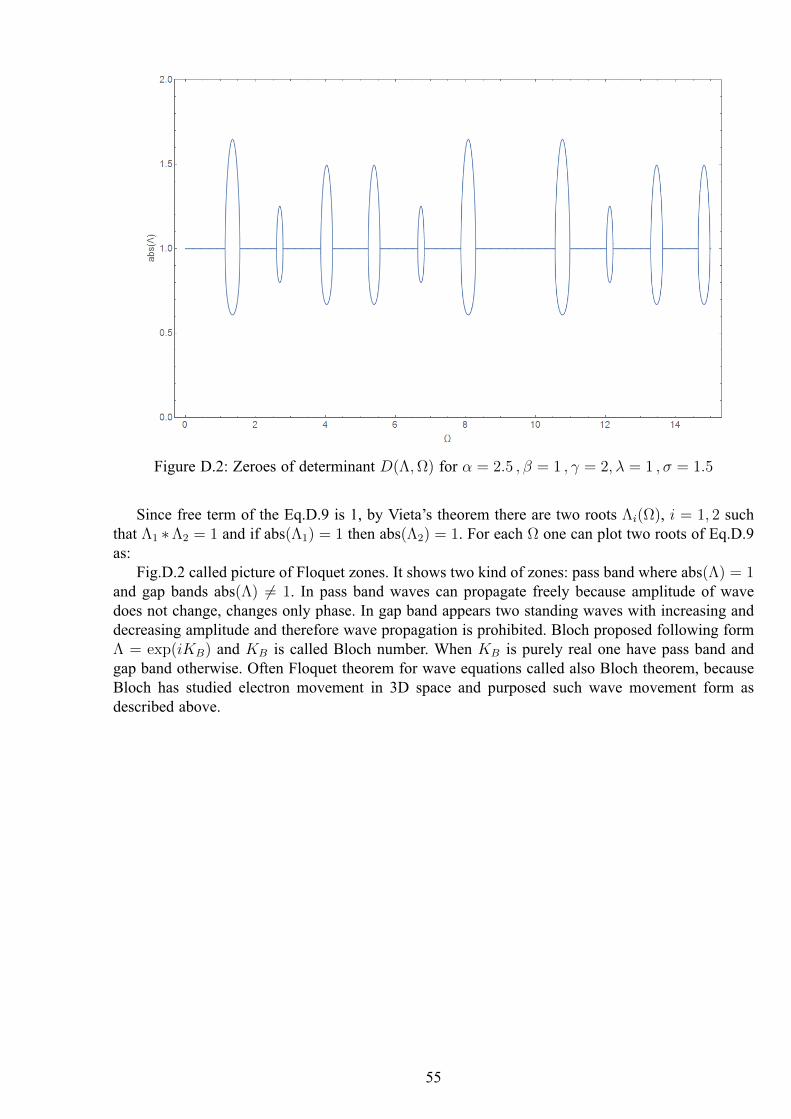
Figure D.2: Zeroes of determinant 𝐷(Λ,Ω) for 𝛼 = 2.5 , 𝛽 = 1 , 𝛾 = 2, 𝜆 = 1 , 𝜎 = 1.5

Since free term of the Eq.D.9 is 1, by Vieta’s theorem there are two roots Λ𝑖(Ω), 𝑖 = 1, 2 suchthat Λ1 *Λ2 = 1 and if abs(Λ1) = 1 then abs(Λ2) = 1. For each Ω one can plot two roots of Eq.D.9as:

Fig.D.2 called picture of Floquet zones. It shows two kind of zones: pass band where abs(Λ) = 1and gap bands abs(Λ) = 1. In pass band waves can propagate freely because amplitude of wavedoes not change, changes only phase. In gap band appears two standing waves with increasing anddecreasing amplitude and therefore wave propagation is prohibited. Bloch proposed following formΛ = exp(𝑖𝐾𝐵) and 𝐾𝐵 is called Bloch number. When 𝐾𝐵 is purely real one have pass band andgap band otherwise. Often Floquet theorem for wave equations called also Bloch theorem, becauseBloch has studied electron movement in 3D space and purposed such wave movement form asdescribed above.

55