Embed Size (px)
Citation preview
ACOUSTIC SENSING FOR METAL TRANSFER MODEAND PENETRATION STATE CLASSIFICATION OFGMAW USING ARTIFICIAL NEURAL NETWORKS
An investigation of the acoustic response of GMAW's capabilities within
machine learning-based weld quality monitoring
By
Anders Bidstrup
Master thesis
M.Sc. Manufacturing Technology
Aalborg University
MAIN REPORT


Study Board of Industry and Global
Business Development
Fibigerstræde 16
DK - 9220 Aalborg Øst
Tlf. 99 40 93 09
www.en.ses.aau.dk
Title:
Acoustic sensing for metal transfer mode
and penetration state classi�cation of
GMAW using arti�cial neural networks
Semester:
VT-4
Project period:
February 2017 - June 2017
ECTS:
30
Anders Bidstrup
Supervisors:
Simon Bøgh
Casper Schou
Censor:
Peter Vangsø Jeberg
Pages: 79
Appendix: 29
Enclosures: 2 pcs.
Synopsis
This report covers a study of the acoustic
response of GMAW's capabilities within ma-
chine learning-based weld quality monitoring.
Initially it is determined to train an arti�cial
neural network, ANN, to classify two metal
transfer modes - globular transfer and short-
circuit transfer - and three penetration states
- lack of penetration, full penetration and ex-
cessive penetration - based on related work.
To do so, 1166 features are extracted for each
window of acoustic signal consisting of a range
of temporal-, spectral shape-, harmonic- and
perceptual features as well as statistical fea-
tures from a wavelet packet decomposition.
Classi�cation data is produced in a robotic
GMAW cell by provoking the desired classi-
�cation states. The acquired data is then pre-
processed and input to a function made to
train 110 ANN con�gurations for 15 combi-
nations of window size and overlap using both
gradient descent with adaptive learning rate,
GDA, and scaled conjugate gradient, SCG,
descent.
Based on the trained ANNs it was concluded
that classi�cation of the three penetration
states was possible for ANNs trained us-
ing SCG and partially possible if they are
trained using GDA. Furthermore, the results
for whether classi�cation of metal transfer
mode is possible were inconclusive but showed
a tendency of correct prediction.
The content of this report is freely available and publication (with source reference) may only take place in
agreement with the authors.


Preface
This report documents the project composed by Anders Bidstrup at the 4th semester on
the master program in Manufacturing Technology at Aalborg University during the period
from the 1st of February 2017 to the 2nd of June 2017.
This being the master thesis, the author has to demonstrate his/her ability to solve
industrial or scienti�c problems within manufacturing engineering and technology. To
accomplish this, research is done on a problem combining concepts within the �elds of
digital signal processing, machine learning and welding where the acoustic signal of gas
metal arc welding's capabilities within weld quality monitoring is investigated.
Reading guide Through the report source references in the form of the Harvard method
will appear and these are all listed at the back of the report. References from books,
homepages or the like will appear with the last name of the author and the year of
publication in the form of [Author, Year].
Figures and tables in the report are numbered according to the respective chapter. In
this way the �rst �gure in chapter 3 has number 3.1, the second number 3.2 and so on.
Explanatory text is found under the given �gures and tables. Figures without references
are composed by Anders Bidstrup.
v


Dansk resumé
I denne rapport er der foretaget et studie af MIG/MAG-svejsnings akustiske respons med
henblik på at fastslå dets evner inden for kvalitetsmonitorering af svejsning.
Baseret på et litteraturstudie, er det indledningssvist bestemt, at et neuralt netværk
skal trænes til at klassi�cere to typer af materialeoverførsel - dråbeoverførsel og kort-
slutningsoverførsel - og tre gennembrændingsniveauer - mangelfuld gennembrænding, fuld
gennembrænding og overdreven gennembrænding. For at gøre dette er 1166 karakteristika
udregnet for hvert vindue af et akustisk signal. Disse karakteristika består af en række
tidsmæssige-, spektrale-, harmoniske- og perceptuelle karakteristika såvel som statistiske
karakteriska fra en wavelet packet decomposition.
Klassi�kationsdataen er produceret ved hjælp af en MIG/MAG robotcelle ved at frempro-
vokere de ønskede klasser. Den opsamlede data er herefter pre-processeret og brugt som
input i en funktion til træning af de neurale netværk. Denne træner 110 forskellige neurale
netværk for 15 kombinationer af vinduesstørrelse og overlap ved brug af både gradient
descent with adaptive learning rate, GDA, og scaled conjugate gradient descent, SCG.
Baseret på de trænede neurale netværk blev det konkluderet, at klassi�kation af de tre
gennembrændingsniveauer er muligt ved brug af neurale netværk optimeret med SCG.
Samtidig er det konkluderet, at samme klassi�kation er delvis mulig ved brug af neurale
netværk optimeret med GDA. Derudover var resultaterne ufyldestgørende for, hvorvidt
klassi�kation af materialeoverførsel er mulig. De trænede neurale netværk viste dog en
tendens til at kunne forudsige de korrekte klasser.
vii

Table of contents
Nomenclature 1
Introduction 3
Chapter 1 Welding theory 5
1.1 The GMAW process . . . . . . . . . . . . . . . . . . . . . . . . . . . . . . . 5
1.2 Quality of a weld . . . . . . . . . . . . . . . . . . . . . . . . . . . . . . . . . 14
1.3 Discussion . . . . . . . . . . . . . . . . . . . . . . . . . . . . . . . . . . . . . 16
Chapter 2 Signal Theory 17
2.1 Digital signals . . . . . . . . . . . . . . . . . . . . . . . . . . . . . . . . . . . 17
2.2 Acoustic data . . . . . . . . . . . . . . . . . . . . . . . . . . . . . . . . . . . 17
2.3 Digital signal processing . . . . . . . . . . . . . . . . . . . . . . . . . . . . . 19
Chapter 3 Machine learning overview 27
3.1 Machine learning algorithms . . . . . . . . . . . . . . . . . . . . . . . . . . . 27
3.2 Training an algorithm . . . . . . . . . . . . . . . . . . . . . . . . . . . . . . 27
3.3 Evaluating hypothesis . . . . . . . . . . . . . . . . . . . . . . . . . . . . . . 30
3.4 Discussion . . . . . . . . . . . . . . . . . . . . . . . . . . . . . . . . . . . . . 31
Chapter 4 Related work 33
Chapter 5 Problem speci�cation 35
Chapter 6 Method 37
Chapter 7 The arti�cial neural network 39
Chapter 8 Experimental setup and data collection 41
8.1 Experimental setup . . . . . . . . . . . . . . . . . . . . . . . . . . . . . . . . 41
Chapter 9 Experiment design and execution 49
9.1 Experiment design . . . . . . . . . . . . . . . . . . . . . . . . . . . . . . . . 49
9.2 Procedure and settings . . . . . . . . . . . . . . . . . . . . . . . . . . . . . . 50
9.3 Sources of variance . . . . . . . . . . . . . . . . . . . . . . . . . . . . . . . . 52
9.4 Identifying conversion rates . . . . . . . . . . . . . . . . . . . . . . . . . . . 55
9.5 Identifying penetration state and mode settings . . . . . . . . . . . . . . . . 55
9.6 Classi�cation data acquisition for penetration states . . . . . . . . . . . . . 58
9.7 Classi�cation data acquisition for transfer modes . . . . . . . . . . . . . . . 60
Chapter 10 Data analysis 61
10.1 Data labelling . . . . . . . . . . . . . . . . . . . . . . . . . . . . . . . . . . . 61
10.2 Removal of improper classi�cation data . . . . . . . . . . . . . . . . . . . . 62
ix

10.3 Filtering . . . . . . . . . . . . . . . . . . . . . . . . . . . . . . . . . . . . . . 63
10.4 Feature extraction . . . . . . . . . . . . . . . . . . . . . . . . . . . . . . . . 64
Chapter 11 Model training and performance evaluation 67
11.1 Procedure . . . . . . . . . . . . . . . . . . . . . . . . . . . . . . . . . . . . . 67
11.2 Results . . . . . . . . . . . . . . . . . . . . . . . . . . . . . . . . . . . . . . . 71
Chapter 12 Discussion 77
Chapter 13 Conclusion 79
Chapter 14 Perspectives 81
14.1 Perspectives . . . . . . . . . . . . . . . . . . . . . . . . . . . . . . . . . . . . 81
List of Figures 85
List of Tables 89
Bibliography 91
Appendix A Quality inspection methods
Appendix B Digital signals
Appendix C Digital �ltering
Appendix D Algorithm overview
Appendix E ANN structure and functionality
Appendix F LabView program
Appendix G Identifying conversion rates
Enclosure A Robotcontroller Interface for FLEX 4000
Enclosure B Matlab program for feature extraction and ANN training
Nomenclature
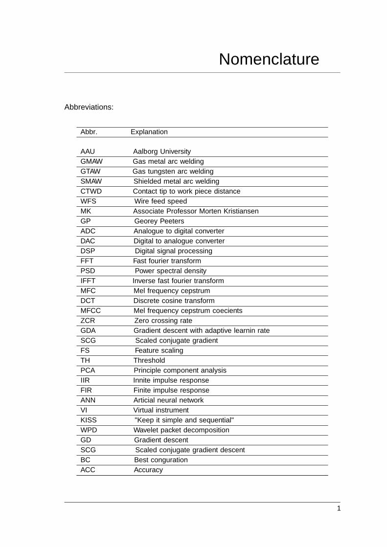
Abbreviations:
Abbr. Explanation
AAU Aalborg University
GMAW Gas metal arc welding
GTAW Gas tungsten arc welding
SMAW Shielded metal arc welding
CTWD Contact tip to work piece distance
WFS Wire feed speed
MK Associate Professor Morten Kristiansen
GP Geo�rey Peeters
ADC Analogue to digital converter
DAC Digital to analogue converter
DSP Digital signal processing
FFT Fast fourier transform
PSD Power spectral density
IFFT Inverse fast fourier transform
MFC Mel frequency cepstrum
DCT Discrete cosine transform
MFCC Mel frequency cepstrum coe�cients
ZCR Zero crossing rate
GDA Gradient descent with adaptive learnin rate
SCG Scaled conjugate gradient
FS Feature scaling
TH Threshold
PCA Principle component analysis
IIR In�nite impulse response
FIR Finite impulse response
ANN Arti�cial neural network
VI Virtual instrument
KISS "Keep it simple and sequential"
WPD Wavelet packet decomposition
GD Gradient descent
SCG Scaled conjugate gradient descent
BC Best con�guration
ACC Accuracy
1
Anders Bidstrup Table of contents
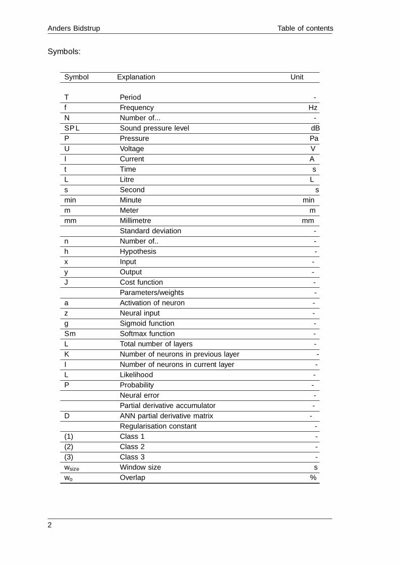
Symbols:
Symbol Explanation Unit
T Period -
f Frequency Hz
N Number of... -
SPL Sound pressure level dB
P Pressure Pa
U Voltage V
I Current A
t Time s
L Litre L
s Second s
min Minute min
m Meter m
mm Millimetre mm
σ Standard deviation -
n Number of.. -
h Hypothesis -
x Input -
y Output -
J Cost function -
θ Parameters/weights -
a Activation of neuron -
z Neural input -
g Sigmoid function -
Sm Softmax function -
L Total number of layers -
K Number of neurons in previous layer -
I Number of neurons in current layer -
L Likelihood -
P Probability -
δ Neural error -
∆ Partial derivative accumulator -
D ANN partial derivative matrix -
λ Regularisation constant -
(1) Class 1 -
(2) Class 2 -
(3) Class 3 -
wsize Window size s
wo Overlap %
2
Introduction
In turn with the rise of the global market, the pressure for western manufacturers to
perform has increased. The entry of manufacturing companies based in countries with
lower production costs has lowered the prices of products and forced western manufacturing
companies to either relocate, outsource parts of their production or in other ways reduce
their production cost. Consequently business philosophies have surfaced to aid in the �ght
for competitiveness often focusing on eliminating waste in the form of time and materials
leading to an increased demand for process monitoring and control.
In order to perform control of a process e�ectively a monitoring model of the given system
is developed to produce reference values for the process stability. Developing this model can
be time consuming requiring extensive knowledge about the given process as well as about
general process modelling within the �elds the given process. The alternative comes with
the rise of machine learning. Through mathematical algorithms a computer can automate
the process modelling making a previously tedious and expensive task doable with data
analytics and programming as the only prerequisites for a wide range of applications.
As one of the primary joining processes, welding plays a signi�cant role in the
manufacturing industry. Especially gas metal arc welding, henceforth GMAW, has due
to its capability for automation, versatility, speed and low cost found its place as the most
used welding process in industry. Therefore it would be advantageous for the industry to
be able to monitor and control the GMAW process. However, the process involves many
sources of variance making the traditional modelling method ine�ective and has over the
years therefore lead to the use of machine learning. As early as around year 2000 papers
document that voltage and current monitoring in combination with machine learning
algorithms made it possibly to identify penetration status in GMAW [Di et al., 2000] [Feng
et al., 2002]. Alongside the continuous improvement of technology the feature space started
to include more process features including features based on human sense mimicking. It
is intuitively understandable that welders rely on their sight and touch to perform a job.
This has inspired researches to develop machine vision for welding applications to monitor
aspects such as the molten pool of material [Baskoro et al., 2011], seam geometry [Xiuping
et al., 2014] etc. Less intuitively is the fact that welders' performance rely on their auditory
sense, which was not properly investigated until a study by Joseph Tam and Jan Huissoon
in 2005, which proved a correlation [Tam and Huissoon, 2005]. Consequently research
regarding the use of the acoustic signal of welding processes for quality monitoring has
surfaced.
In this report the acoustic response of GMAW's capabilities in machine learning-based
weld quality monitoring is investigated.
3


Welding theory 1In this chapter basic welding theory and an explanation of the GMAW process is presented.
Furthermore ISO-5817: Welding - Fusion-welded joints in steel, nickel, titanium and their
alloys (beam welding excluded) - Quality levels for imperfections is presented alongside an
explanation of how the process variance is controlled in manual GMAW.
1.1 The GMAW process
In this section the basics of GMAW is presented.
1.1.1 Equipment and terminology
In order to explain how GMAW works, it is necessary to be familiar with the general
equipment used in the process and its related terms. The following list of equipment is
provided alongside �gure 1.1 to provide an idea of the setup.
Figure 1.1: The required setup to perform gas metal arc welding [Hera, 2017].
� Arc
An electric arc is a heat generating electrical discharge between an anode and catode
separated by a layer of gas.
� Work piece
The work pieces of a welding process are the pieces of metal to be joined and function
as the catode in the creation of the electric arc.
� Electrode wire
The electrode wire serves as both the anode in the creation of the electric arc and
as the �ller material of the weld.
� Weld
The weld refers to the created joint between two work pieces.
5

Anders Bidstrup 1. Welding theory
� Gas shield
The gas shield is provided to protect the molten weld pool from mainly oxygen and
water vapour.
� Welding gun
The welding gun is what the welder controls during the welding process, hereby
determining the position of the weld as well as when to activate and deactivate gas
�ow and wire feed.
� Nozzle
The end of the welding gun is denoted the nozzle. It supplies the wire electrode as
well as the gas for the gas shield.
� Wire feed unit
The wire feed unit supplies the welding gun with a continuous �ow of electrode wire.
� Gas shielding supply
The gas shielding supply supplies the welding gun with a continuous �ow of shielding
gas.
� Power source
The power source supplies the electric current needed to create the arc.
To gain an understanding as to how the equipment works together to produce a weld, a
process description is given.
1.1.2 Process description
In order for a weld to be generated during GMAW, an arc needs to be struck. This happens
by providing the work piece with an electric current and creating contact with the wire
electrode fed by the welding gun. The heat generated by the arc melts the wire electrode
which causes a material transfer to take place. Since the arc also heats up part of the work
piece a molten weld pool is created consisting of both work piece and �ller material. Once
cooled, the �ller material has melted together with part of each work piece hereby creating
the joint known as a weld.
As suggested by the name, the process includes the use of gas. To be speci�c, an inert
or semi-inert gas is used to shield the molten weld pool mainly from oxygen and water
vapour. The gas is provided by an external supply, feeding it to the welding gun that
through the nozzle creates the wanted atmosphere around the weld.
1.1.3 Types of welds
When speaking of types of welds, the topic can be divided into two areas - joint type and
weld groove type.
The joint type refers to how the two work pieces are going to be joined and is because of
this rarely an aspect to be changed after the product design is �xed. A selection of the
most common joint types is shown on �gure 1.2.
6

1.1. The GMAW process Aalborg University
Figure 1.2: A range of joint types in welding [Kristiansen, 2007].
Some of the joint types shown on �gure 1.2 are either classi�ed as or can be made as a
groove weld. A groove weld indicates that there is a groove to be �lled during the welding
process, see �gure 1.3 A, and is the counterpart to the �llet weld where no groove is present
as indicated on �gure 1.3 B.
Figure 1.3: (A) A groove weld and (B) a �llet weld.
A joint type as butt weld is always a groove weld. However, the simple square groove is
not always su�cient for the task at hand. To cope with more situations multiple groove
types are available and are shown in �gure 1.4.
Figure 1.4: A range of weld groove types [Wikiwand, 2017].
Each type of groove has a range of suitable applications making it necessary to investigate
and conclude on what type of groove is most suitable for the given job.
1.1.4 Oscillation
During a weld it is sometimes necessary to perform an oscillation pattern. In the case of
no oscillation the welder simply welds in a straight line along the weld axis. When an
oscillation pattern is applied, variation in the gun position takes place along the weld axis.
To illustrate the concept, a range of oscillation patterns are shown on �gure 1.5.
7

Anders Bidstrup 1. Welding theory
Figure 1.5: A range of oscillation patterns [Marlow, 2012].
The patterns shown on �gure 1.5 indicate the attack point of the welding gun along a
weld, going from the left and following the arrowed line. As the oscillation patterns on
the �gure indicate, the possibilities when it comes to choosing an oscillation pattern are
endless and each have di�erent results. Which pattern to choose is highly situational and
should be investigated prior to any weld.
1.1.5 Metal transfer modes
In GMAW the wire melts and thereby transfers metal to the work piece. Depending
on the input parameters the way of transferring material is di�erent. Three overall
transfers modes are considered and explained in this section based on an article from
The Fabricator [FMA communications, 2008].
Short-circuit transfer mode
In short-circuit transfer mode the wire is allowed to reach the work piece without melting
even though an arc is established. Once the wire is in contact with the work piece, the
system is short-circuited causing the arc to extinguish and the wire to heat up and undergo
pinching, see �gure 1.6 (A). The pinching involves a necking process of the wire which
eventually ends up with a molten piece of wire being transferred to the work piece and an
arc being established, see �gure 1.6 (B).
8

1.1. The GMAW process Aalborg University
Figure 1.6: Short-circuit GMAW with (A) illustrating the contact, heat build-up andpinching of the wire and (B) illustrating the arc and molten transferred material on thework piece [Wall Mountain Company, 2002].
This mode is generally enabled when using a voltage below 22 V [Wall Mountain Company,
2002].
Globular transfer mode
In contrast to short-circuit transfer mode, the arc is always active in globular transfer mode.
In this case the heat of the arc causes the wire to melt before getting into contact with
the work piece. Consequently globs of molten wire material breaks o� and is transferred
to the work piece as shown on �gure 1.7.
Figure 1.7: Globular transfer with molten globs of wire material being transferred to thework piece through the arc [Wall Mountain Company, 2002].
The globs are usually larger than the diameter of the wire and can exit the arc resulting
in excessive spatter. This mode is generally enabled when using a voltage of more than 22
V, a current of less than the transition current speci�ed in the article by The Fabricator
and a shielding gas consisting of either 100 % CO2 or an argon and CO2 mix is used [Wall
Mountain Company, 2002].
Spray transfer mode
Similar to globular transfer, spray transfer does not result in contact between wire and
work piece. The metal is still transferred in globs but in the case of spray transfer
9

Anders Bidstrup 1. Welding theory
these are usually smaller than the diameter of the wire and more frequent, see �gure 1.8.
Furthermore the globs are restricted to the arc reducing spatter.
Figure 1.8: Spray transfer with molten globs being transferred to the work piece throughthe arc [Wall Mountain Company, 2002].
The di�erence compared to globular transfer lies in the choice of shielding gas and current.
Although the mode is enabled using a voltage of more than 22 V, a current above the
transition current speci�ed in the article by The Fabricator and requires the use of
an argon and CO2 mix shielding gas with an argon content of more than 80 % [Wall
Mountain Company, 2002].
1.1.6 Control parameters
In order to monitor and control GMAW it is required to have an understanding as to which
parameters a�ect the process. This report uses the classi�cation of parameters derived by
Associate Professor Morten Kristiansen, henceforth MK, at AAU in appendix L: taxonomy
of generic information model of his PhD thesis from 2007 [Kristiansen, 2007]. From these
parameters a sub-set, which contains suitable controlling parameters, is chosen and the
conclusion as to which to consider in this project is presented.
In �gure 1.9 a part of the set of parameters derived by MK is shown.
10

1.1. The GMAW process Aalborg University
Figure 1.9: Part of the set of welding parameters derived by MK [Kristiansen, 2007].
11

Anders Bidstrup 1. Welding theory
As indicated on �gure 1.9, the parameters are split up into six main groups
� Work piece parameters
The constant parameters throughout the work piece.
� Equipment parameters
The parameters that describe the used equipment.
� Work piece variables
The parameters that vary along the weld axis.
� Process variables
The parameters to be measured throughout the process.
� Welding control variables
The parameters used to control the weld.
� Quality parameters
The parameters that indicate the quality of the weld.
Inspecting the total set of parameters it is clear that some are more suitable for controlling
the system. Initially all parameters contained in Work piece parameters, Equipment
parameters and Work piece variables are disregarded with the exclusion of gas �ow rate.
The remaining parameters are determined prior to a welding task and require either
design or equipment changes, which is the basis for the assessment to disregard them
as control parameters. Furthermore, both the process variables and quality parameters
are disregarded as direct control parameters. The process variables in the case of MK
are parameters to be measured throughout the process and are thereby, much like the
quality parameters, a consequence of the other parameters contained in the entire six
groups. However, due to this nature these parameters are potential candidates for process
monitoring.
Through the elimination of parameters, the following sub-set is proposed:
� Work angle
� Travel angle
� Rotational angle
� CTWD
� Sideway
� Travel speed
� Voltage
� Wire feed speed
� Gas �ow rate
� Oscillation on
� Oscillation vector X
� Oscillation vector Y
� Oscillation vector Z
� Oscillation width
� Oscillation frequency
� Oscillation holding 1
� Oscillation holding 2
� Oscillation holding centre
� Oscillation pattern
To provide further understanding of the parameters they are explained individually.
12

1.1. The GMAW process Aalborg University
Angles
In the sub-set three angles appear - work-, travel- and rotational angle. An overview of
these can be seen on �gure 1.10.
Figure 1.10: An overview of the angles and axes found in a weld [Kristiansen, 2007].
As indicated on �gure 1.10, the axis along the weld is denoted Xgroove, the axis along the
width of the work piece is denoted Ygroove and the axis perpendicular to the plane de�ned
by Xgroove and Ygroove is denoted Zgroove. Using this terminology the angles can now be
explained.
The work angle is de�ned as the angle between Zgroove and Ygroove, the travel angle is
de�ned as the angle between Zgroove and Xgroove and the work angle is the rotation around
Zgroove.
Contact tube to work piece distance
The contact tube to weld distance, henceforth CTWD, is the distance from the contact
tube to the weld.
Sideway
The sideway is the line onto which the welding guns point of attack is. Should it be
necessary to change the point of attack, it moves along this line.
Travel speed
The speed at which the welder moves the weld gun along the weld axis.
13

Anders Bidstrup 1. Welding theory
Voltage
The voltage set on the welding equipment.
Wire feed speed
The speed at which the wire is fed to the welding gun.
Gas �ow rate
The rate at which the gas �ows to the welding gun.
Oscillation on
A binary parameter to de�ne whether an oscillation pattern is chosen. If set to 0, the
remaining parameters in the control parameter set are disregarded.
Oscillation parameters
The rest of the parameters in the control parameter set are used to de�ne the nature of
the oscillation pattern chosen for the process.
1.2 Quality of a weld
In this section the possible imperfections of a weld is presented alongside an introduction
to how the quality of a weld is determined in practice and how control is performed in
practice in manual welding.
1.2.1 Welding imperfections
Whether the quality of a weld is satisfactory is ultimately determined by whether the
weld lives up to the set of speci�cations given by the customer in the form of aesthetic or
functional requirements. Both of these aspects are evaluated according to the presence of
welding defects or imperfections. Because of this ISO-5817 exists to aid in determination
of the quality level of a weld. [DanskStandard, 2014].
The standard speci�es four groups of guidelines in regards to quality checking. The groups
are enumerated and named as follows:
� 1.0 Surface imperfections
� 2.0 Internal imperfections
� 3.0 Imperfections in joint geometry
� 4.0 Multiple imperfections
For reference, each guideline is speci�ed by a number preceded by the group number, e.g.
2.12: Lack of fusion being the 12th internal imperfection. A short description of each
group of guidelines is given with examples from the standard. For further elaboration on
the speci�c guidelines, the author refers to the standard.
14
1.2. Quality of a weld Aalborg University
Surface imperfections
This group contains the guidelines for imperfections on the surface. In order to provide
a graspable introduction to these a grouping of imperfections is made. The grouping
resulted in the imperfections being divided into surface cracks, surface pores, end-geometry
imperfections and penetration imperfections.
In terms of surface cracks and pores the names are self-explanatory. Furthermore it is
speci�ed that the presence of surface cracks is not permitted under any circumstance
while pores can be allowed in some cases based on the wanted quality level and pore size.
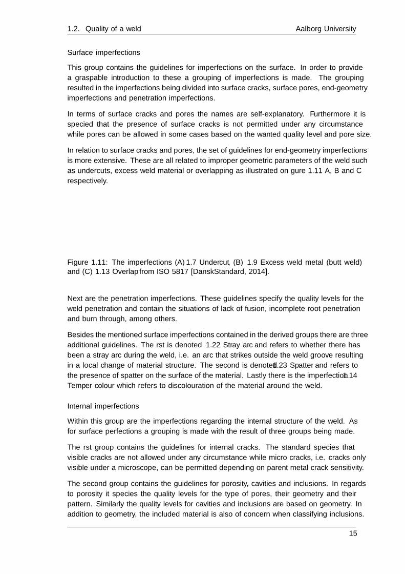
In relation to surface cracks and pores, the set of guidelines for end-geometry imperfections
is more extensive. These are all related to improper geometric parameters of the weld such
as undercuts, excess weld material or overlapping as illustrated on �gure 1.11 A, B and C
respectively.
Figure 1.11: The imperfections (A) 1.7 Undercut, (B) 1.9 Excess weld metal (butt weld)
and (C) 1.13 Overlap from ISO 5817 [DanskStandard, 2014].
Next are the penetration imperfections. These guidelines specify the quality levels for the
weld penetration and contain the situations of lack of fusion, incomplete root penetration
and burn through, among others.
Besides the mentioned surface imperfections contained in the derived groups there are three
additional guidelines. The �rst is denoted 1.22 Stray arc and refers to whether there has
been a stray arc during the weld, i.e. an arc that strikes outside the weld groove resulting
in a local change of material structure. The second is denoted 1.23 Spatter and refers to
the presence of spatter on the surface of the material. Lastly there is the imperfection 1.14
Temper colour which refers to discolouration of the material around the weld.
Internal imperfections
Within this group are the imperfections regarding the internal structure of the weld. As
for surface perfections a grouping is made with the result of three groups being made.
The �rst group contains the guidelines for internal cracks. The standard speci�es that
visible cracks are not allowed under any circumstance while micro cracks, i.e. cracks only
visible under a microscope, can be permitted depending on parent metal crack sensitivity.
The second group contains the guidelines for porosity, cavities and inclusions. In regards
to porosity it speci�es the quality levels for the type of pores, their geometry and their
pattern. Similarly the quality levels for cavities and inclusions are based on geometry. In
addition to geometry, the included material is also of concern when classifying inclusions.
15

Anders Bidstrup 1. Welding theory
Lastly the third group contains internal penetration imperfections. The two imperfections
found in this group are lack of fusion and internal lack of penetration. As the names
suggest, lack of fusion is the situation where the �ller material is not fused together with
the work piece whereas internal lack of penetration is the situation where the weld does
not go deep enough into the weld groove.
Imperfections in joint geometry
Within this group are the imperfections regarding the joint geometry. More speci�cally it
contains guidelines for work piece misalignment or incorrect root gaps for �llet welds.
Multiple imperfections
Lastly this group provides guidelines for the case of multiple imperfections.
1.2.2 Quality inspections
Generally quality control is divided into two groups - non-destructive, henceforth NDT, and
destructive, henceforth DT. An overview of popular NDTs and DTs is given in appendix A.
1.3 Discussion
Based on the presented welding theory and the purpose of this report, it is determined
that square grooved butt-joint welds is to be investigated in this project. The decision
is based on the simplicity of the joint design and the assessment that it is suitable for
the extraction of evidence regarding the research topic of machine learning driven quality
monitoring based on acoustic emission.
In order to select a �tting set of quality parameters a study of which imperfections have
a unique acoustic response should be performed. Based on these results, adequate quality
tests can be determined through the methods listed in appendix A.
16

Signal Theory 2In this chapter the basics of digital signals, acoustic data and digital signal processing,
henceforth DSP, is presented.
2.1 Digital signals
In order to perform monitoring, output data is to be obtained from a range of sensors.
Although the purpose for the report is to monitor and control the process through acoustic
data, other signals can be used to aid the process. Based on their vital role in the stability
of the process and in�uence on the generated sound during GMAW, see chapter 4, current
and voltage could be acquired to help understand the process and indicate changes.
The equipment required to acquire the voltage, current and sound have one thing in
common which is that they convert an analogue signal to a digital signal. An introduction
to the distinction of analogue and digital signal as well as the terminology used for digital
signals and the possible pitfalls of the acquisition is presented in appendix B. Based on
the information presented in the appendix, key features to be aware of during the data
acquisition is the bit resolution and sample frequency. The resolution should be chosen
so that its full range is utilised without the equipment capping. Furthermore the sample
frequency should be chosen so that the desired frequencies to be observed can be extracted.
2.2 Acoustic data
As the primary output of the welding process in this project the acoustic signal needs to
be captured and processed to identify discriminative features. In this section the digital
representation of sound is presented.
2.2.1 Sound
To gain an understanding of what equipment to use in acoustic data acquisition it is
required to understand sound. The information presented in this section is based on the
lecture notes from Gerald Penn from University of Toronto [Penn, 2010].
Sound is de�ned as a mechanical wave moving through a given medium and created by
the vibration of an object. The medium can be anything, i.e. metal, water, gasses, and,
as in the case of this report, air. The energy produced by the arc sets the particles of the
surrounding air in motion making them oscillate between compressions and rarefactions
as indicated by �gure 2.1.
17

Anders Bidstrup 2. Signal Theory
Figure 2.1: A sound wave in a medium. The alternation between compression andrarefactions within the air is indicated by C and R respectively [Penn, 2010].
The wave illustrated on �gure 2.1 is called a longitudinal wave. Furthermore it should
be noted that sound can be represented by a single or combination of sine functions as
indicated by the pressure-time graph on �gure 2.1.
To describe a wave the frequency and amplitude should be known. The frequency of
the wave is the amount of complete back-and-forth motions, i.e. periods, is present in
the medium per unit of time. It is denoted f and has the unit Hz. Depending on the
mechanism to pick up the sound di�erent frequency ranges can be measured. In the case
of the human ear the audible frequency range is said to be between 20 Hz and 20 000
Hz [BBC, 2014]. The human ear is simply not capable of picking up signals outside this
range, however sound in the non-audible range for humans still exist. Commonly the
domain with frequencies below 20 Hz is denoted infra sound whereas the domain above 20
000 Hz is denoted ultra sound.
As for the amplitude, it is the work done to generate the energy that sets the particles
in motion and is shown as the displacement from equilibrium on an amplitude-time
graph [Penn, 2010].
The intensity of sound is measured in decibel, dB. It is presented on a logarithmic scale
and tells the ratio for comparing two sounds in intensity. For an interpretable unit a
�xed pressure of 2 · 105 is de�ned as the reference for 0 dB, P0, which corresponds to the
threshold of hearing [Penn, 2010]. Using this reference the absolute sound pressure, P , can
be calculated as 20 log10(P/P0). For reference table 2.1 shows a list of sound intensities.
Intensity Reference0 dB Threshold of hearing20 dB Quiet living room40 dB Refrigerator60 dB Normal conversation90 dB Passing motorcycle100 dB Somebody shouting110 dB Loud rock concert120 dB Pain threshold
Table 2.1: Reference activities for levels of sound intensity [Penn, 2010].
18

2.3. Digital signal processing Aalborg University
2.3 Digital signal processing
Seeing as a signal is a quantity varying in time, it is in some cases necessary to extract
features from the data to describe the signal. One of these cases could be to e�ectively
distinguish between two signals, e.g. in certain machine learning algorithms. For the
distinction to be made it is elementary that discriminating features are extracted from the
signals which is why understanding how to synthesise, transform and analyse these is key.
Being aspects of the �eld of DSP this section aims to present su�cient information as to
how this is performed.
2.3.1 Segmenting
In DSP assignments the basic operation of segmenting is often used when analysing signals
whose characteristics vary over time. By expressing the signal as a series of segments with
their own properties, a piece-wise understanding of the signal is obtained. To perform the
segmentation, the concept of windowing is introduced.
Windowing
The process of windowing is performed by letting a window pass through a signal in the
time domain by using a so-called window function. A window function is de�ned by being
real-valued within a �nite range of inputs and zero-valued outside the given range. By
applying this function on a signal, a segment is cut and scaled through the values speci�ed
in the real-valued part of the window. In order to perform windowing, three parameters
need to be considered - type, length and overlap.
The type of window is determined by the shape and magnitude of the values applied to
the signal during the window length. Two typical windows are shown in �gure 2.2.
0 0.5 1 1.5 2 2.5 3
Time [s]
-0.2
0
0.2
0.4
0.6
0.8
1
1.2
Am
plitu
de
(A) Rectangular window
0 0.5 1 1.5 2 2.5 3
Time [s]
-0.2
0
0.2
0.4
0.6
0.8
1
1.2
Am
plitu
de
(B) Hamming window
Figure 2.2: A (A) rectangular and (B) Hamming window in the time frame going fromt = 1 to t = 2.
For both graphs the window function is set to have its e�ect between t = 1 and t = 2. On
�gure 2.2 (A) a rectangular window is shown. As indicated it has the value zero outside the
window space and a constant value of one during the length of the window. Employed on a
signal it merely cuts out a segment of the signal since the data is scaled equally by a factor
of one throughout the window. Alternatively a Hamming window is shown on �gure 2.2
(B). This type of window has a bell shape with the tails ending in a value of 0.08. By
19

Anders Bidstrup 2. Signal Theory
doing so, every part of the window has a weight in contrast to having the tails reaching
zero. With the curve at the top of the graph and the tails decreasing on either side, the
function weights the data in the center of the window the most, while moving away from
the center to either side entails a decrease in the weight of the data. Determining the
type of window to use depends on applications and should be considered before each DSP
operation where a window function is used.
The length of the window is as the name suggests how long the window should be.
Having the signal as samples, the length is de�ned as how many samples are included
in the window. The choice of length entails di�erent results when doing DSP so careful
consideration should be taken before a decision is made.
Besides the type of length of the window, overlapping may be introduced. The overlap
is a parameter to determine how much of the previous window should be included in the
current window and is denoted in percent. Examples of overlap is seen in �gure 2.3.
0 0.5 1 1.5 2
Time [s]
0
0.2
0.4
0.6
0.8
1
Am
plitu
de
(A) 0% overlap
0 0.5 1 1.5 2
Time [s]
0
0.2
0.4
0.6
0.8
1
Am
plitu
de
(B) 20% overlap
Overlap
0 0.5 1 1.5 2
Time [s]
0
0.2
0.4
0.6
0.8
1
Am
plitu
de
(C) 40% overlap
Overlap
Figure 2.3: Two consecutive Hamming windows with an overlap of (A) 0%, (B) 20% and(C) 40%.
20

2.3. Digital signal processing Aalborg University
Illustrated on �gure 2.3 are two consecutive Hamming windows with 0%, 20% and 40%
overlap respectively. Moving the window through a signal using an overlap has an averaging
e�ect since an amount of data from the previous window is included in the current one -
an e�ect which can be bene�cial in DSP operations.
Lastly the choice of window length and overlap de�nes the amount of segments the signal
is split into, denoted nw, the e�ect of which is speci�c to the DSP operation in progress.
2.3.2 Signal domains
In the �eld of DSP so-called domains exist the most common of which being time domain
and frequency domain. The transition between domains occur through signal transforms
and each domain provides a set of features to be extracted.
Time domain
When acquiring a signal it is obtained as a set of values through time as mentioned in
section 2.1, i.e. the signal is captured in the time-domain. A signal in the time domain is
usually presented as a time series as seen in �gure 2.4.
0 2 4 6 8 10 12 14 16 18
Time
-1
-0.5
0
0.5
1
Am
plitu
de
sin(x)
Figure 2.4: sin(x) in the time domain.
Having a signal in the time-domain allows analysis of speci�c values, e.g. through
descriptive statistics, and time-dependent features, i.e. temporal features. Having a
signal in the time domain makes it possible to spot trends in the data and allows for
pinpointing moments in time where speci�c situations occur. However, it does not present
an overview of which frequencies are present in the signal, which can aid in the description
and synthesising of signals. To gain this information a transformation is made to transfer
the signal to the frequency domain.
Frequency domain
Transforming a signal from time-domain to frequency-domain happens through a spectral
decomposition. The idea behind this builds on the assumption that any signal can be
expressed as a combination of sine functions with di�erent frequencies. The way of
determining the frequencies of these sine functions is done by performing a discrete fourier
transform or the more computationally e�cient version called fast fourier transform,
henceforth FFT. The result of this is a complex-valued function of frequency. Taking
the square magnitude of the function provides values that describe how much power of a
21
Anders Bidstrup 2. Signal Theory
given frequency bin is present in the signal. The set of these powers is called the power
spectral density, henceforth PSD, and is plotted in what is known as a power spectrum
or periodogram which can be described through e.g. peak analysis or spectral shape
descriptors.
Along with any sampled signal comes the disadvantage of it being imperfect and being a
�nite set of data. Consequently the calculated PSD is an estimation riddled with noise.
Due to this Peter D. Welch developed a method to reduce the e�ect of the noise in a trade-
o� with frequency resolution [Welch, 1967]. Instead of calculating the PSD for the entire
data set, it is subjected to windowing, usually with a Hamming window, before creating a
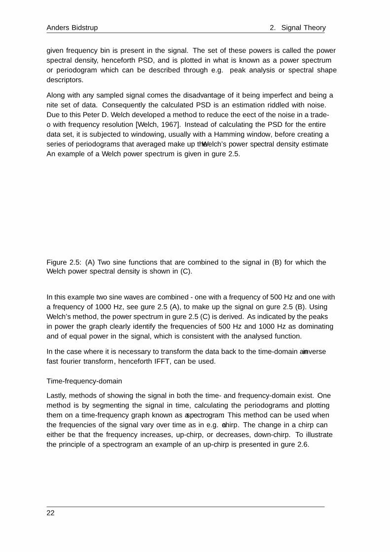
series of periodograms that averaged make up the Welch's power spectral density estimate.
An example of a Welch power spectrum is given in �gure 2.5.
0 0.5 1 1.5 2
Time [s] ×10-3
-2
-1
0
1
2
Am
plitu
de
(A) Individual sine functions
500 Hz1000 Hz
0 0.5 1 1.5 2
Time [s] ×10-3
-2
-1
0
1
2
Am
plitu
de
(B) Combined sine functions
0 1 2 3
Frequency (kHz)
-100
-80
-60
-40
-20
0
Pow
er/fr
eque
ncy
(dB
/Hz)
(C) Welch Power Spectral Density Estimate
Figure 2.5: (A) Two sine functions that are combined to the signal in (B) for which theWelch power spectral density is shown in (C).
In this example two sine waves are combined - one with a frequency of 500 Hz and one with
a frequency of 1000 Hz, see �gure 2.5 (A), to make up the signal on �gure 2.5 (B). Using
Welch's method, the power spectrum in �gure 2.5 (C) is derived. As indicated by the peaks
in power the graph clearly identify the frequencies of 500 Hz and 1000 Hz as dominating
and of equal power in the signal, which is consistent with the analysed function.
In the case where it is necessary to transform the data back to the time-domain an inverse
fast fourier transform, henceforth IFFT, can be used.
Time-frequency-domain
Lastly, methods of showing the signal in both the time- and frequency-domain exist. One
method is by segmenting the signal in time, calculating the periodograms and plotting
them on a time-frequency graph known as a spectrogram. This method can be used when
the frequencies of the signal vary over time as in e.g. a chirp. The change in a chirp can
either be that the frequency increases, up-chirp, or decreases, down-chirp. To illustrate
the principle of a spectrogram an example of an up-chirp is presented in �gure 2.6.
22

2.3. Digital signal processing Aalborg University
0 0.02 0.04 0.06 0.08 0.1
Time [s]
-1
-0.5
0
0.5
1
Am
plitu
de
Up-chirp
0 0.1 0.2 0.3 0.4 0.5
Frequency (kHz)
10
20
30
40
50
60
70
80
90
Tim
e (m
s)
Spectrogram
-110
-100
-90
-80
-70
-60
-50
-40
-30
Pow
er/fr
eque
ncy
(dB
/Hz)
Figure 2.6: (A) The time-domain signal of an up-chirp going from 0 Hz to 500 Hz within0.1 second and (B) its corresponding spectrogram.
In the example shown on �gure 2.6, an up-chirp is generated with a start frequency of 0
Hz at t = 0 and an end frequency of 500 Hz at t = 0.1, see �gure 2.6 (A). To illustrate the
change in frequency the corresponding spectrogram is calculated and presented in �gure 2.6
(B) where it is clear that the frequency increases linearly through time from 0 Hz to 500
Hz in the speci�ed time span, which is consistent with the analysed function.
As the case for the transformation back to time domain, an IFFT for each segment of time
can be performed.
2.3.3 Digital �ltering
When obtaining or synthesising a signal the data is not always as expected. It can be
riddled with noise or have certain frequencies that is not desired for the given process at
hand. Therefore preprocessing of the data is used to modify the data to be more useful.
The process of doing so often requires a form of �ltering. The �ltering can be done either
as an analogue or digital process, but since digital �ltering is not subject to the same
restrictions as analogue �ltering it is decided to only consider digital �lters in this report.
For an introduction to the the basics of �ltering, see appendix C.
2.3.4 Feature extraction
Being able to transform a signal between time- and frequency domain as well as
implementing digital �lters provide the basics of DSP. To better understand how to
discriminate between signals, this section presents an introduction to feature extraction.
It should be noted that only instantaneous features, i.e. short-time features, are presented
since global features are assessed to not provide a bene�cial e�ect to the machine learning
aspect of this project.
This section is based on the work of Geo�roy Peeters, henceforth GP, [Peeters, 2004] in
which a large set of audio features is presented. To illustrate the feature extraction process
and the necessary transforms, the author propose the �gure seen on �gure 2.7.
23

Anders Bidstrup 2. Signal Theory
Figure 2.7: An overview of the feature extraction process presented in [Peeters, 2004]
As indicated by �gure 2.7, GP classi�es the features in the following groups:
� Temporal features
� Spectral shape features
� Harmonic features
� Perceptual features
Furthermore a range of energy features are considered in both the harmonic analysis and
from the signal frame. Note that global temporal descriptors can be extracted from both
the energy envelope and temporal modelling. These are not presented in this section as it
focuses on the extraction of instantaneous features. From �gure 2.7 the feature extraction
process is as follows:
1. The original signal is segmented into frames
2. Temporal features are extracted
3. FFT is performed on each segment
4. Spectral shape features are extracted
5. A sinusoidal harmonic model is derived
6. Harmonic features are extracted
7. A perceptual model is derived
8. Perceptual features are extracted
By performing these steps both the time domain and frequency domain are well covered
and provides features known to be useful in speech recognition.
Temporal features
Temporal features are extracted from the time-series data of a signal segment. Due to
intuitive sense of the type of data and the fact that no transformation is necessary the
majority of temporal features are relatively simple to extract and understand compared
24

2.3. Digital signal processing Aalborg University
to spectral features. One range of features focus on the distribution of the amplitudes
in a signal segment through descriptive statistics. Others are time-dependent and involve
calculating the frequency of which an event occurs such as the zero-crossing rate, henceforth
ZCR, which measures the amount of time the signal crosses zero within the signal segment.
Spectral shape features
Once the FFT has been performed on the signal, the frequency spectrum of the signal
segment is found. Similarly to the descriptive statistics used in the time domain, the
spectral shape can be described through similar features. Examples of these features
are the spectral centroid, spectral spread and spectral skewness. Furthermore spectral
temporal features can be extracted by comparing the spectrum of consecutive signal
segments through e.g. normalised cross-correlation.
Harmonic features
Using the spectrum of the signal segment harmonic features can be extracted. These
include calculating the fundamental frequency, noisiness and inharmonicity of the signal.
Perceptual features
A perceptual model of the signal can be derived through e.g. mel-frequency cepstrum,
henceforth MFC [cryptography, 2012]. To obtain the MFC, the spectrum for a signal is
calculated and subjected to a mel �lterbank, which is a set of 20-40 triangular �lters spaced
using the mel-scale. After applying the mel �lterbank, the energy for each �lter is computed
as the sum of powers. Taking the logarithm to the �lterbank energies and performing the
DCT results in what is denoted the mel-frequency cepstral coe�cients, henceforth MFCC,
which have shown promising results for auditory weld quality monitoring as mentioned in
chapter 4.
2.3.5 Discussion
In this section the focus of feature extraction has been on audio. However, the features
serve as general descriptors for signals and can be used for e.g. current and voltage data.
Deriving a perceptual model such as the MFC allows for the extraction of features which
refer more to the way a human perceives sound. Seeing as the inspiration from this
report comes from the fact that welders use their auditory sense to determine process
stability [Tam and Huissoon, 2005], extracting perceptual features seems promising and
should be investigated.
25


Machine learning overview 3In this chapter an overview of machine learning is given. Speci�cally a classi�cation of
algorithms is presented alongside a general introduction to how a hypothesis is trained and
evaluated.
3.1 Machine learning algorithms
In machine learning algorithms, i.e. mathematical procedures, are used to automatically
build models. This means that for a given problem it is necessary for the user to determine
what the �nal model should predict and based on what type of data. Once determined, a
suitable algorithm is chosen after which the model is trained, evaluated and evaluated.
Machine learning dates back to around year 1950 and countless algorithms have been
developed from then to now [Marr, 2016]. Consequently the selection of algorithms
has become inconceivable and lacks proper grouping - a task made cumbersome by the
trend of developing task-speci�c algorithms. However, individuals have tried to group the
algorithms and for the case of this project, the method of representation follows Dr. Jason
Brownlee's classi�cation [Brownlee, 2013]. He proposes a grouping based on style and
similarity both of which are presented in appendix D. Although extensive, the list is not
exhaustive but provides insight into the possibilities of the �eld.
3.2 Training an algorithm
Once an algorithm is chosen it is used to train a model. Depending on the algorithm
the training process may vary and all cases are not presented in this section. However the
process presented in this section is widely used and presents the general approach of model
training via machine learning algorithms.
Generally the training process consists of the following steps:
1. Determine hypothesis
2. Determine cost function
3. Minimise cost function
This section is inspired by the Stanford University courseMachine Learning led by Andrew
Ng [Ng, 2017].
27

Anders Bidstrup 3. Machine learning overview
3.2.1 Determining the hypothesis
The hypothesis is the function or model, h(x), that maps the input, denoted x, to the
output, denoted y. In other words, it is the model to be trained to make the best possible
prediction or mapping based on the training data. Determining the hypothesis depends
on the chosen algorithm and multivariate linear regression is used as an example in this
report to illustrate the process. The related hypothesis is:
hθ(x) =n∑i=0
θixi | x0 = 1
with the θ's all being constant parameters or weights, n being the number of features
used and the convention of x0 being set to one. It should be noted that the hypothesis is
subscripted based on weight notation which is why it in this case is subscripted with a θ.
3.2.2 Determining the cost function
The cost function is denoted J and is de�ned di�erently based on the data provided.
In labelled data generally it is an expression of the di�erence between the hypothesis'
prediction and the training data output, while for unlabelled data the algorithms use
more speci�c cost functions. Continuing the case of multivariate linear regression the cost
function can be set to the half the sum of squared di�erences:
J(θ) =1
2m
m∑i=1
(hθ(x(i))− y(i))2
with m being the number of training examples.
3.2.3 Minimising the cost function
With the cost function determined the next step is to minimise. By minimising the cost
function in relation to the weights, the hypothesis is trained to predict the output with
the smallest error. For this the gradient descent method can be used but more advanced
optimisation methods can be implemented if necessary. The formula is written as:
minimiseθ
J(θ) =1
2m
m∑i=1
(hθ(x(i))− y(i))2
and functions by updating all weights simultaneously using a speci�ed learning rate, α, in
the direction of the negative gradient of the cost function in a given point. It should be
noted that the direction of negative gradient is always orthogonal to the contour line at the
point in which it is computed. This may cause a zig-zag phenomenon in the optimisation
problem, which in some cases may lead to slower convergence. The updating formula is:
θj = θj − αδ
δθjJ(θ)
Assuming the learning rate was chosen correctly, a local or global optimum is reached over
the course of a �nite amount of iterations depending on the initial guess of the weights
and the convexity of the problem.
When working with gradient descent one should be aware of the impact of the learning
rate and di�erently scaled features.
28

3.2. Training an algorithm Aalborg University
Gradient descent learning rate
In regards to the learning rate it is important to choose the right value. The in�uence of
α is shown on �gure 3.1.
0 2 4 6 8 10
θ
0
5
10
15
20
25
30
35
J(θ)
(A) α too small
0 2 4 6 8 10
θ
0
5
10
15
20
25
30
35
J(θ)
(B) α too big
Figure 3.1: The iterations of a minimisation task with the asterisk marking the startingvalue. Examples of (A) slow convergence due to small α and (B) divergence due to largeα.
Choosing a learning that is too small results in slow convergence as seen on �gure 3.1 (A)
and should be made larger to improve performance. Having the learning rate too large
will cause the function to diverge and thereby never reach the optimum as indicated on
�gure 3.1 (B). Therefore choosing the learning rate should be done with care.
Feature scaling
When the used features are on di�erent scales attention should also be paid. An increasing
degree of di�erence between the scales of two features increase the rate of convergence for
the minimisation. To handle this e.g. feature scaling can be used. The principle of this is
to make the scales similar by scaling them to be in in the same range. An example of this
could be through the following formula:
x(i)fs =
x(i) −min(x)
max(x)−min(x)
with xfs denoting the feature scaled input. By using this formula for the input, they are all
converted to the range of 0 to 1, which may improve the rate of convergence and prediction
accuracy compared to the raw state.
3.2.4 Over�tting vs under�tting
When training a model it is important to handle the problem of over�tting and under�tting.
The problem is illustrated for a housing price example in �gure 3.2.
29

Anders Bidstrup 3. Machine learning overview
Figure 3.2: Exmaples of (A) under�tting and (B) over�tting on a housing priceexample [Ng, 2017].
On �gure 3.2 (A) the case of under�tting is shown. As indicated the �t is a bad match
since it does not accurately predict the price for the training data. On �gure 3.2 (B) the
case of over�tting is shown. Here the hypothesis accurately predicts the price in the exact
point of the training data but fails to model the tendency of the data making it inaccurate
on cases di�erent from the training data. To combat this regularisation is used.
Regularisation
Regularisation is a term added to the cost function and included in the optimisation process
to combat �tting errors. The term is:
λ
N∑j=1
θ2j
with λ being the regularisation constant and N being the amount of features. It should be
noted that the summation starts at j = 1 since the parameter θ0 should not be scaled. As
indicated by the term, it multiplies the squared sum of weights by a value of λ to control
the e�ect of them on the hypothesis. By using a large value of λ the weights assume small
values and hereby makes the hypothesis less prone to over�tting. Using a too large value
however, causes the hypothesis to become a constant. Because of this regularisation can
be used to reduce �tting errors, but λ should be chosen carefully.
3.3 Evaluating hypothesis
Once the hypothesis is trained to �t the training data there is a method of evaluating its
performance. It consists of testing the hypothesis on data not in the data set. One way
of obtaining test data is to split the acquired data set into a training set and a test set.
The hypothesis is then trained on the training set and tested on the remaining data set
to provide a measure of performance. However, only training on one data set may lead to
over�tting.
To better secure the performance of a hypothesis the data set can be split into three
section - training set, test set and validation set. By having three sets another loop in the
30

3.4. Discussion Aalborg University
optimisation can be implemented. In the case of doing polynomial regression the outer
loop could choose the degree of the polynomial. In this case the procedure is as follows:
1. Optimise the weights for each polynomial degree on the training set
2. Calculate the error of the hypotheses on the validation set
3. Choose the degree of polynomial based on lowest validation error
4. Calculate the error of the hypothesis on the test set
Making the outer loop decide the degree of polynomial results in a better generalised �t
which then, similarly to the method with two sets, can be used to calculate a performance
measure on the data from the test set. A rule of thumb for the splitting of the data is to
use 60%, 20% and 20% of the original data set to create the training-, validation- and test
set respectively.
Other evaluating tactics exist to determine the performance of the hypothesis and proposed
actions to improve it looking into bias and variance cases as well as learning curves.
3.4 Discussion
Based on the knowledge presented in this report it seems �tting to use a supervised
classi�cation algorithm for the quality monitoring of GMAW.
31

Related work 4Researchers have investigated the acoustic response of welding processes since the 1940's.
During the years of research it has been concluded that the primary in�uences on the
sound generated during GMAW are the arc behaviour, molten pool dynamics, droplet
transfer, shielding gas and welding equipment [Saini and Floyd, 1998] [Grad et al., 2003].
In short this means that the arc stability can be measured in the sound which suggests
that welding defects caused by or causing instability of the arc can be detected. Since the
transfer mode of a GMAW process a�ects the voltage and current signal, and in turn the
arc, it is possible to detect which transfer mode is active during the weld as investigated
by E. H. Cayo and S. C. Absi Alfaro in 2008 [Cayo and Alfaro, 2008].
So far the majority of research focus on identifying the penetration state on �at butt welds
with a process generally consisting of data acquisition, feature extraction, dimensionality
reduction and algorithm choice.
Data acquisition
Since the inspiration for investigating the acoustic signal of welding has its roots within
human hearing sense mimicking there is a wide agreement to use microphones with a
frequency range within the hearing range of humans, i.e. 20 Hz - 20 000 Hz.
Feature Extraction
In order to train a given machine learning algorithm, a range of features must be extracted
from the acoustic data. These features can be found within any of the signal domains,
i.e. time domain, frequency domain etc., and a de�nitive answer as to which to use is
not available. Therefore di�erent combinations of features are investigated often without
limiting to one domain. If gas tungsten arc welding, henceforth GTAW, and shielded
metal arc welding, henceforth SMAW, are considered as well, multiple suggestions as
to which features to use can be found. These suggestions range from simpler solutions
using statistical features from the original time domain signal [A.Sumesh et al., 2015]
or from the nodes of a wavelet packet decomposition [Wang et al., 2011] to more
comprehensive solutions using multiple features from both time-, frequency-, MFC- and
geometry domain [Bi et al., 2010]. The three mentioned papers all succeeded in using
their respective features to classify penetration status which consequently leads to the
conclusion that the acoustic signal of GMAW, GTAW and SMAW indeed can be used for
penetration state classi�cation.
Dimensionality reduction
The use of dimensionality reduction is seen in the article by Shujuan Bi, Hu Lan, Hongyan
Zheng and Lijun Liu from 2010, PCA is used to eliminate redundant features from a
larger set of descriptive parameters [Bi et al., 2010]. In the similar case for GTAW a
33

Anders Bidstrup 4. Related work
large set of features extracted from a wavelet decomposition is reduced using a generic
algorithm [Wang et al., 2011]. In both cases the authors managed to produce models with
an accuracy of 85 % or higher.
Algorithm choice
Since there is no direct answer as to which machine learning algorithm to use for GMAW
monitoring, a wide range of examples can be found. Examples include arti�cial neural
networks [Bi et al., 2010] [Wang et al., 2011] [Lv et al., 2013] and Hidden Markov
Models [Na et al., 2013] as well as decision trees such as J48 and Random Forest [A.Sumesh
et al., 2015]. All proposed algorithms provide an accuracy of more than 70 %.
34
Problem specification 5Throughout chapter 1, chapter 2, chapter 3 and chapter 4 the problem of developing a
quality monitoring system for robotic GMAW based on sound is presented. Consequently
it is decided to look into the transfer modes and penetration state of square grooved butt
welds. A model is to be trained using the acoustic emission of the process leading to the
decision of using a supervised classi�cation algorithm.
Chapter 2 and chapter 4 presents a range of temporal-, spectral-, harmonic- and perceptual
features to extract which may prove useful in the classi�cation process. Especially the
use of perceptual features are of interest since these are extracted from a model closely
resembling the way sound is perceived by humans. Furthermore, research has shown that
the use of descriptive features from the nodes of a wavelet packet decomposition is useful in
the classi�cation of the penetration state of a weld. Lastly chapter 3 and chapter 4 suggests
that a range of algorithms can train models able of prediction penetration state with an
accuracy greater than 70 %. Based on its documented ability to predict the penetration
state of GMAW and its versatility it is decided to further investigate the use of an arti�cial
neural network, henceforth ANN, in penetration state monitoring as well as metal transfer
mode monitoring leading to the following hypothesis and sub-hypotheses:
h1: It is possible to monitor GMAW using an arti�cial neural network trained on
labelled acoustic data
h1.1: It is possible to identify the penetration state of GMAW through its acous-
tic emission using an arti�cial neural network
h1.2: It is possible to identify the metal transfer mode of GMAW through its
acoustic emission using an arti�cial neural network
To specify the problem further a range of delimitations are determined:
� The use of oscillation patterns is not considered
� Investigating the process of welding with oscillation patterns is not considered
for this project.
� Other gasses than Mison 18 are not considered
� Mison 18 is available and suitable for the project. Other gasses could be used
but including these in the investigation is beyond the scope of this report.
� Other metals than steel are not considered
� Other metals could be used but including these in the investigation is beyond
the scope of this report.
35

Anders Bidstrup 5. Problem speci�cation
� Other wire materials or types are not considered
� Other wire materials and types could be used but including these in the
investigation is beyond the scope of this report.
� Other type of welds or grooves are not considered
� Other types of welds or grooves could be investigated but including these in the
investigation is beyond the scope of this report.
� Other types of weld geometries are not considered
� Other types of weld geometries could be investigated but including these in the
investigation is beyond the scope of this report.
36
Method 6In order to either accept or reject the hypotheses in chapter 5, evidence is produced to
support the claims. The method developed to do so consists of the following steps:
� Specify the type of ANN
� Modify the current experimental setup
� Perform experiments
� Analyse data
� Extract features
� Train ANN
� Evaluate performance
Each point is elaborated further in this chapter.
Specify the type of ANN
The �rst step of testing the hypotheses is to specify the type of ANN and fully understand
the structure, hypothesis, cost function and training method.
Modify the experimental setup
To gain an understanding of the limitations and usage of the existing setup, an analysis of
the current hardware and software is required. Once understood, a data acquisition system
must be made so that the voltage, current and sound can be logged at an appropriate rate
and quality.
Perform experiments
Once the algorithm is speci�ed and the data acquisition system is implemented,
experiments can be made. The settings of the process are speci�ed and preventive actions
to reduce variance are applied to ensure the quality of the experiments. Afterwards
experiments are performed to obtain data for each classi�cation case.
Analyse data
The acquired data from the experiments is labelled so that it can be used for supervised
learning. In the process of doing so unwanted sections of the data are removed in an
attempt to reach maximum prediction accuracy. If further preprocessing of the data is
required, this should also be performed before feature extraction.
37

Anders Bidstrup 6. Method
Extract features
Having the labelled data available, the feature extraction can begin. Which features to
include should be considered and how to extract them presented. Once determined the
data can be segmented according to a speci�c type and length of window with as well as
the size of the overlap, after which the chosen features can be extracted. Once completed,
the feature vectors for each segment is given the label of the data from which the segment
is cut, consequently leading to two matrices for each hypothesis - an input feature matrix,
x, and a labelled output matrix, y.
Train ANN
Using the input and output matrix found during the feature extraction, the ANNs can be
trained. Before doing so it should be considered whether normalisation would boost the
prediction accuracy of the model.
Evaluate performance
Having trained the neural networks confusion matrices are used to provide an overview of
the accuracy of the classi�er. Lastly the evaluation of the ANNs is used to assess whether
the hypotheses are accepter or rejected.
38
The artificial neuralnetwork 7
In this chapter the choice of neural network is presented including elaboration on the choice
of optimisation method and cost function.
Speci�cally the type of network used is a backpropagation network using a cross-entropy
cost function. For a detailed description of the general structure and functionality of the
speci�ed ANN, see appendix E.
Structure
Generally no guideline for the structure of a neural network is given. Therefore di�erent
structures should be analysed during training and the best network con�guration chosen.
Choice of optimisation
It is assessed that the use of gradient descent is su�cient for the ANN training performed
in this project. The method is simple to implement and a popular choice of optimisation
method for neural networks. However, as explained in chapter 3, the choice of learning
rate of the optimisation method is crucial to the performance of the method. Therefore
the introduction of an adaptive learning rate is used. This is done by implementing a
punishment/reward-system based on the performance of the optimisation. Speci�cally
if the newest cost exceeds the previous cost by a pre-de�ned ratio, the newly calculated
weights are disregarded, the step size is decreased and the weights are recalculated. Should
the newest cost not exceed the previous cost the step size is increased. This method is
known as gradient descent with adaptive learning rate, henceforth GDA.
Alternatively the use of scaled conjugate gradient descent, henceforth SCG, could be
investigated. This optimisation method is not learning rate dependent and proven to
increase convergence rate [Moeller, 1991]. The main improvement lies in the fact that
where the gradient descent can only take steps in the orthogonal direction of the contour
line, see chapter 3, the SCG can step in any direction. By doing so, the optimum can
be reached without the zig-zag steps performed in gradient descent and possibly handle
non-convex problems more e�ectively.
Choice of cross-entropy
A commonly known cost function is the mean square error, see chapter 3, proven to work
perform well for linear regression. However, for the case of logistic regression, such as the
case of ANNs using sigmoid activation functions, the cost function would be non-convex
39

Anders Bidstrup 7. The arti�cial neural network
due to the degree of non-linearity [Ng, 2017]. This means that the cost has multiple
local minima and in that way does not guarantee convergence to the global minimum. To
counteract this, cross-entropy is used, since it produces a convex optimisation problem [Ng,
2017]. Based on its known e�ect in logistic regression, cross-entropy is a popular choice of
cost function in neural networks. This is done despite the fact that the multiple logistic
regressions performed in an ANN makes the optimisation problem non-convex. However,
based on its popular usage, it is chosen to use cross-entropy in this project.
The speci�c type of cross-entropy used in this report is based on the use of a Softmax
output activation function. In order to function properly, the labelled data should be
one-hot encoded as explained in appendix E.
40

Experimental setup anddata collection 8
In this chapter the experimental setup and the modi�cation made to perform the required
data acquisition is presented.
8.1 Experimental setup
To perform robotic GMAW AAU has provided a cell with the necessary equipment. Onto
this equipment a range of sensors have been implemented and a data acquisition system
is developed. To provide an understanding of the complete setup, this section initially
presents the robotic GMAW equipment followed by a presentation of the hardware and
software of the data acquisition system.
8.1.1 The robotic GMAW setup
The setup is shown on �gure 8.1.
Figure 8.1: The available setup at Aalborg University.
As indicated on the �gure the equipment consists of the following items:
� Gas system
� Flex 4000 Migatronic welding equipment
� Welding gun + cable
� Ground clamp + cable
41

Anders Bidstrup 8. Experimental setup and data collection
� Robot controller
� Migatronic control box
� ABB robot
� Microphone
� Welding �xture
The gas system, Flex 4000 Migatronmic welding equipment, welding gun, welding gun
cable, ground clamp and ground clamp cable are connected as speci�ed in section 1.1.
The gripper of the ABB robot holds the welding gun and is equipped with a stand
for the microphone. Control of the robot and welding equipment happens through the
robot controller which sends the signals directly to the robot and indirectly to the welding
equipment through the Migatronic control box. Furthermore the Migatronic control box
acquires the actual voltage and current of the welding equipment at a sample rate of 1 Hz.
To provide deeper understanding of the equipment each module is described in detail.
Welding equipment
The welding equipment is provided by Migatronic and is of the type Flex 4000 [Migatronic,
2017]. It can deliver a wire freed speed of 1 - 24 mmin , a current of 5 - 500 A and sets the
voltage automatically. Inside a drum of 1.2 mm rutile �ux-cored wire [welding, 2013] is
mounted and the machine is fed gas from an external source.
Gas system
The gas system consists of a gas cylinder, a regulator and a manometer. In the gas cylinder
there is Mison 18 [AGA, 2015] which is a gas consisting of primarily ≈18 % CO2 and ≈82% argon. Going from the cylinder to the welding equipment, the gas passes through a
regulator onto which a manometer is mounted. On the regulator the �ow of gas can be
changed and the actual �ow is measured and shown on the manometer.
ABB robot
The robot is made by ABB and is of type IRB 140 [ABB, 2017]. It has 6 degrees of
freedom allowing it to control the work-, travel- and rotational angle as well as perform
the required movement for the process. It is controlled through a supplied robot controller
that reads RAPID programs. A hand held pendant is used to perform online programming
and alternatively programs can be written on a computer and send to the controller via
FTP connection. The robot controller also communicates with the Migatronic control
box. The controller enables the user to move the robot to a di�erent point in space with
a speci�ed speed and an option to specify rounding of path between separate movements
is available. Furthermore it has speci�c inputs for welding denoted as seam-, weld- and
weave data is speci�ed.
In the case of this report both seam- and weave data is disregarded leaving the weld data
in which the WFS, voltage and travel speed of the weld is speci�ed.
The robot is mounted with a gripper to hold the welding gun and has an attachment onto
which a microphone can be mounted, see �gure 8.2.
42

8.1. Experimental setup Aalborg University
Figure 8.2: The ABB robot holding the welding gun and the attachment to the gripperholding a microphone.
Migatronic control box
The Migatronic control box sends and acquires signals from the welding equipment and
communicates to the robot controller. The terminals of the control box are explained
in the data sheet, see enclosure A. The box controls the welding equipment by activating
WFS, gas �ow, voltage and current once triggered. The signal for WFS and current ranges
from 0 - 10 V and translates to a WFS of 0 - 24 mmin or current of 0 - 400 A. The signal
for voltage also ranges from 0 - 10 V and translates to an actual voltage of 0 - 100 V.
Lastly the control box has terminals which output the measured voltage and current of
the welding equipment.
Microphone
The microphone is from Projects unlimited and is of type AOM-6738P-R [unlimited, 2006].
The sensitivity of the microphone is stable between 20 Hz and 2 000 Hz after which its
stability decreases going towards 20 000 Hz. However, it allows the acquisition of the
frequencies in the human auditory range. Extra features of the microphone include being
omnidirectional, meaning it can capture sound from all directions, and having distortion-
free response.
Welding �xture
The welding �xture was designed and produced as part of this project and is shown on
�gure 8.3.
43

Anders Bidstrup 8. Experimental setup and data collection
Figure 8.3: The welding �xture.
As shown on �gure 8.3 (A), the �xture consists of two section of a square pipe welded to
a plate onto which six circular stops are welded to guide the work pieces. It is designed
to leave a gap of 2 mm between two work pieces of 75 mm width. Onto the plate is also
welded two sections of a U-pipe to allow welding clamps to secure the plates once on the
�xture, see �gure 8.3 (B). The entire �xture is �xed to the work table with two bolts in
countersunk holes to secure its position in case of dis- and reassembly.
8.1.2 The data acquisition setup
It is decided to acquire both voltage, current and sound from the process. Sound is acquired
from the microphone while voltage and current is acquired both from the Migatronic control
box and newly installed sensors on the welding equipment. The low sample frequency of the
measurement of voltage and current in the Migatronic control box makes the signal unable
to e�ectively capture the characteristic events of the voltage and current as explained in
chapter 4. Therefore a voltage probe and current sensor is installed on the equipment and
sampled at a higher frequency.
The full data acquisition setup is shown on �gure 8.4.
44
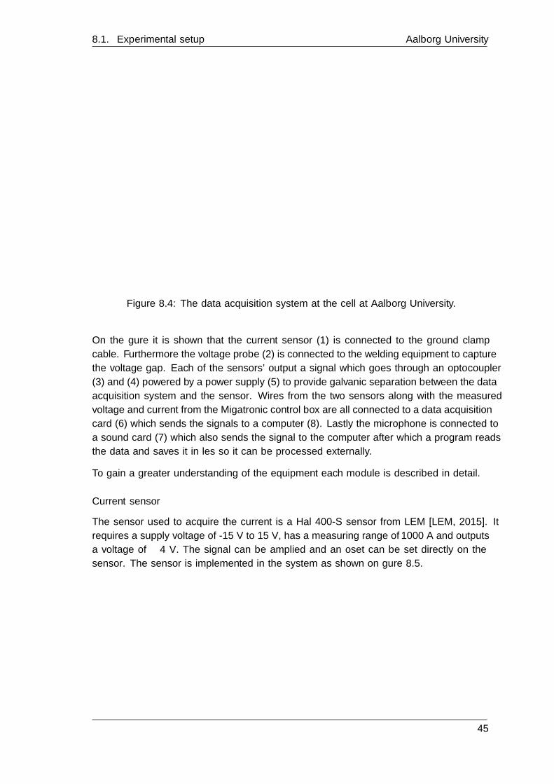
8.1. Experimental setup Aalborg University
Figure 8.4: The data acquisition system at the cell at Aalborg University.
On the �gure it is shown that the current sensor (1) is connected to the ground clamp
cable. Furthermore the voltage probe (2) is connected to the welding equipment to capture
the voltage gap. Each of the sensors' output a signal which goes through an optocoupler
(3) and (4) powered by a power supply (5) to provide galvanic separation between the data
acquisition system and the sensor. Wires from the two sensors along with the measured
voltage and current from the Migatronic control box are all connected to a data acquisition
card (6) which sends the signals to a computer (8). Lastly the microphone is connected to
a sound card (7) which also sends the signal to the computer after which a program reads
the data and saves it in �les so it can be processed externally.
To gain a greater understanding of the equipment each module is described in detail.
Current sensor
The sensor used to acquire the current is a Hal 400-S sensor from LEM [LEM, 2015]. It
requires a supply voltage of -15 V to 15 V, has a measuring range of ± 1000 A and outputs
a voltage of ± 4 V. The signal can be ampli�ed and an o�set can be set directly on the
sensor. The sensor is implemented in the system as shown on �gure 8.5.
45

Anders Bidstrup 8. Experimental setup and data collection
Figure 8.5: The Hal sensor set to measure the current through a wire connected to thework table and the ground clamp.
As indicated on the �gure, the ground clamp is mounted to a piece of wire mounted to
the work table. The Hal sensor is mounted on the piece of wire to measure the current
running through the system.
Voltage probe
The voltage probe was included in the purchase of the setup and of an unspeci�ed producer.
It takes an input of 0 - 100 V and converts it to a 0 - 10 V signal.
Optocoupler system
The two optocouplers are of type PR 2284 [electronics, 2017a]. Although they have other
functions, the function used in this report is to obtain galvanic separation between the
sensors and the data acquisition system. Depending on type they take a di�erent input
and provide di�erent outputs. The ones chosen in this project are type E6 which takes an
input of 0 - 10 V and outputs 0 - 10 V. They require a power supply of 24 VDC which is
provided by a PR 2220 [electronics, 2017b]. It is a switch mode power supply and enables
the use of the two optocouplers.
Data acquisition card
The data acquisition card is from National Instruments and is called NI USB-6216 M
series [NationalInstruments, 2009]. It is a 64 screw terminal card with the possibility to
both input and output analogue signals and transfers data through a USB connection to
a computer which also acts as its power supply. For inputs it has an aggregate or single
channel sample frequency of 400 kSs , an ADC resolution of 16 bit and take inputs ranging
from ± 10 V. For outputs it has an update rate of 250 kSs , a DAC resolution of 16 bit and
outputs signals of ± 10 V.
46

8.1. Experimental setup Aalborg University
Sound card
The sound card used is Edirol UA-25 [RolandCorporation, 2004]. It connects to a
microphone through XLR connection, has two channels, a 24 bit resolution and a sample
rate of 96 kHz. It communicates with the computer through USB connection from which
it is also powered.
Software
The data from the data acquisition card and sound card is sent to the computer through
USB. Since National Instruments has their own data acquisition program, LabView, it is
decided to use this for data acquisition.
The developed LabView program alongside a description of its structure and functionality
is found in appendix F.
47


Experiment design andexecution 9
In this chapter the experiments to perform are designed and executed. Initially an
introduction to good practice in experiments is given followed by a speci�cation and result
presentation for each performed experiment.
9.1 Experiment design
To ensure the quality of the performed experiments one must be methodical and consistent.
This section aims to highlight how to perform and which factors a�ect the quality of
experiments using the work of Douglas C. Montgomery [Montgomery, 2012].
9.1.1 A good experiment
Any designed experiment should follow the principle of KISS, i.e. Keep it small and
sequential. This means that presented with a complex task it should be broken down into
smaller experiments performed sequentially. In the case of this report it is necessary to map
a feature space based on sound to a the penetration state of GMAW and its metal transfer
modes. To do so it is chosen to work with supervised learning which in turn means that
the need for labelling the data is present. To gain su�cient knowledge about the feature
space the individual penetration states and metal transfer modes must be provoked so
their respective data can be logged and used for training the model. However, being a
complex process it is unclear in which ranges of the input values the desired penetration
states and transfer modes are provoked. In this case using the KISS principle would be
bene�cial to separate the identi�cation of the required values and the actual classi�cation
data acquisition.
Besides using the KISS model it is important to know the di�erence between controllable
variables and uncontrollable variables. Controllable variables are process parameters such
as voltage, current and WFS which can be changed on demand. In contrast uncontrollable
variables can not be easily changed such as work piece thickness and environmental factors.
For a good experiment it is important to minimise the e�ect of uncontrollable variables
and to have control over the controllable variables' variance, i.e. having variable control.
9.1.2 Discussion
Seeing as the goal of the experiments in this report is complex, it is decided to use the
KISS principle. Doing so has lead to a composition of four experiments:
49

Anders Bidstrup 9. Experiment design and execution
� Identifying conversion rates
� Identifying penetration state and transfer mode settings
� Classi�cation data acquisition for penetration states
� Classi�cation data acquisition for transfer modes
In the composition the initial experiment involves determining the correct conversion rates
for the implemented sensors. In the second experiment settings for provoking penetration
states and transfer modes are found so that the classi�cation data for the case of identifying
penetration states and transfer modes can be performed.
9.2 Procedure and settings
A range of variables are held constant during the experiments and are therefore out
of consideration in the experiments. These parameters and the basic procedure of the
experiments are explained in this section.
9.2.1 Settings
The input parameters are voltage, WFS and travel speed. However, as presented in
chapter 1, the welding process is a�ected by a range of other parameters. The settings
used for these experiments are presented in table 9.1.
50

9.2. Procedure and settings Aalborg University
Parameters/variables ValueWork piece parameters
Material plate 1 S235JRMaterial plate 2 S235JRStart temperature 22oCEquipment parameters
Gas mixture Mison 18
Gas �ow rate 14 Lmin
Gas nozzle diameter 20 mmWire type Flux-coredWire diameter 1.2 mmWork piece variables
Root gap 2 mmthickness plate 1 3 mmthickness plate 2 3 mmsurface plate 1 Unknownsurface plate 2 UnknownGroove horizontal angle 0Groove vertical angle 0Welding control variables
Work angle 8Travel angle 22Rotational angle 0CTWD 5 mmTravel speed InputVoltage InputWFS InputOscillation on No
Table 9.1: The settings used for the welding experiments.
To clarify how these parameters were chosen an explanation of the work piece parameters
and variables, the equipment parameters and welding control variables is given.
Work piece parameters and variables
The work pieces used for the experiments are 150 mm long sections of 3 mm x 75
mm S235JR metal bars from Sanistål [Sanistaal, 2017] stored at room temperature, i.e.
approximately 22oC. The root gap of 2 mm is chosen on the basis of the rule of thumb in ISO
9692 [DanskStandard] stating that for square butt welds of plates with a thickness below 4
mm a root gap of approximately the thickness of the plate should be used. Following this
rule the root gap should be 3 mm. However, using 1.2 mm diameter wire sets a relatively
high requirement for the energy level in the weld. Consequently the decrease of 1 mm in
the root gap is chosen to lower the probability of burn through. Lastly the surface of the
work pieces are not considered in this project and since the work pieces are parallel to the
ground the groove angles are both 0.
51

Anders Bidstrup 9. Experiment design and execution
Equipment parameters
In regards to the equipment parameters no changes have been made to the current setup.
Consequently the gas mixture is Mison 18, the �ow rate is 14 Lmin , the nozzle diameter is
20 mm and the wire is 1.2 mm rutile �ux-cored wire as speci�ed in chapter 8.
Welding control variables
Initially, since the travel speed, WFS and voltage are input variables, no value is given in
table 9.1. In regards to the rotational and work angles these should be zero since the weld
is a �at square butt weld. However, due to limitations of the setup, having a work angle
of 0 is impractical. As a consequence of this the work angle is 8 degrees. The travel angle
and CTWD are determined through initial experiments and set to 22 degrees and 5 mm
respectively. Lastly the binary value for whether the oscillation is on is set to 0 since it
is decided in the problem speci�cation not to investigate the e�ect of oscillation patterns,
see chapter 5.
9.2.2 The experiment procedure
Before the robot performs the full weld, it is decided to tack weld the work pieces. Doing
so reduces the warpage of the plates during the full weld and provides the robot with a
spot to strike the arc in the beginning of the process. The tack welding is done manually
using the �xture presented in section 8.1. Once the work pieces are tack welded, the �xture
is mounted on the work table of the robot cell.
After mounting the �xture the RAPID program for the weld is run without striking an
arc so the path can be checked. Once the path is assessed to be of suitable precision
the settings for the weld is input, the data acquisition program is started and the weld is
performed. Once �nished, the data acquisition is stopped, the work piece is dismounted
from the �xture and numbered according to the name of respective data �les.
9.3 Sources of variance
During the experiments variance is expected in regards to a range of controllable and
uncontrollable variables. These and the preventive actions to minimise their impact is
presented in this section.
9.3.1 Controllable variables
The controllable variables, the cause of their variance and the preventive action to minimise
their variances' e�ect is shown in table 9.2.
52

9.3. Sources of variance Aalborg University
Variable Cause of variance Preventive action
Welding control parameters Internal equipment variance NoneEquipment parametersWork piece Storage temperature Work pieces stored attemperature Heat transfer same temperatureRoot gap Work piece geometry Tack welded in sequence
Fixture geometry by same personTack welding Visual comparison to
template gapGroove horizontal angle Geometry and parallelity of NoneGroove vertical angle work table
Geometry and parallelity of�xture
Table 9.2: Controllable variables, their cause of variance and the preventive action tominimise their e�ect.
As indicated by table 9.2 no preventive action is taken for the welding control parameters,
equipment parameters or groove angles. In regards to the welding control parameters the
decision to not perform a preventive action lies in the fact that it would require online
correction of the parameters or improvement of the equipment which is out of the scope
for this project to develop. For the equipment parameters, preventive actions are not taken
since the variance in gas mixture, wire diameter, nozzle diameter and wire type is assessed
to be of less e�ect relative to the other sources. Lastly no preventive action is taken to
minimise variance of the groove horisontal and vertical angles since they are assessed to
be subject to less variation relative to the other sources.
In regards to the work piece temperature, the problem lies in the fact that the material
properties of the metal changes with temperature. It is assessed that storing the work
pieces in the same room and letting them cool down after tack welding is a su�cient
action to minimise the variance caused by the initial temperature. In regards to the heat
transfer of the process no preventive action is taken.
The last source of variance for the controllable parameters is the root gap. This is
categorised as a controllable variable since manual tack welding is performed. In an
attempt to minimise the e�ect of performing the process manually it is performed in
sequence by the same person. Furthermore, a visual comparison to a template gap size
determines the usability of the work pieces to eliminate outliers.
9.3.2 Uncontrollable variables
Similarly to the controllable variables the name of the variable, the source of its variance
and the preventive action to reduce its e�ect is presented for each uncontrollable variable
in table 9.3.
53

Anders Bidstrup 9. Experiment design and execution
Variable Cause of variance Preventive action
Work piece material Material property variation None
Work piece surface Oxidation, oils, geometry, Nonecoating
Work piece thickness Production method Cut using sawCutting method Deburring of non-welded edges
Allignment of burrs on weldededge
Environment Noise Data acquired past regularTemperature changes work hours
Table 9.3: Uncontrollable variables, their cause of variance and the preventive action tominimise their e�ect.
As shown in table 9.3 no preventive action is taken in regards to work piece material and
surface variance. This decision is made based on the assesment that the materials bought
from Sanistål did not require special attention to reduce these parameters' variance.
Although the work piece thickness mostly refers to the tolerance of the thickness of the
plates the presence of burrs is included in this consideration. Although no preventive
action is taken to reduce the variance of the work piece thickness, several actions are taken
to remove burrs. The burrs come from a combination of cutting by blade and saw. The
steel bars are previously cut into 6 000 mm x 75 mm bands by blade causing the edges to
su�er from a burr on the longitudinal edges, see �gure 9.1 (A).
Figure 9.1: Sketched cross-sectional view of a plate post cutting.
To reduce the variance in the welds caused by this, the plates are placed with the burr
facing downwards for every weld as indicated by �gure 9.1 (B). The process of cutting
metal with a blade also has the disadvantage of causing the material to warp. However,
it is assessed not to be necessary to take preventive action to minimise this variance. To
prevent further warpage it is decided to cut the steel bars using a saw when sectioning the
6 000 mm steel bar into 150 mm sections. Furthermore the burrs caused by the saw is
removed after sectioning.
In regards to the environment, variance is caused by noise and temperature changes. These
e�ects are mainly present when the area around the robot cell is subject to people working
or passing through. To reduce the e�ect of these sources all data was acquired outside
regular work hours under quiet, stable conditions.
54

9.4. Identifying conversion rates Aalborg University
9.4 Identifying conversion rates
An experiment is performed to determine the conversion rates from the voltage probe and
current sensor. The experiments are speci�ed and documented in appendix G. Based on
the results from the experiments, conversion rates were implemented in the data acquisition
system in order to acquire the actual voltage and current of the process.
9.5 Identifying penetration state and mode settings
In this section a range of experiments are performed to identify settings at which the
di�erent transfer modes and penetration states occur.
9.5.1 Speci�cation
In regards to provoking the di�erent metal transfer modes it is known from the theory
presented in section 1.1.5 that the limit between short-circuit transfer and globular/spray
transfer lies at 22 V. The transfer mode should not be a�ected by the travel speed which is
why it is held constant through the experiments. Although the high argon gas of Mison 18
is suitable for provoking spray transfer it is assessed that an investigation of spray transfer
is out of consideration. The decision is based on the fact that the work pieces used are 3
mm thick steel with a root gap of 2 mm which puts a limitation in the amount of heat put
into the weld and therefore cant exceed the transition current as explained in section 1.1.5.
Since the original setting of the welding equipment is approximately 22 V the settings used
in the experiments are as shown in table 9.4.
Travel speed Voltage WFS1 0 01 2 -21 4 -41 -2 21 -4 4
Table 9.4: The settings used to provoke short-circuit and globular transfer.
It should be noted that the settings are the adjustments made to the default settings of
the welding equipment. By using the settings displayed in table 9.4 a coarse breaking
point for the transfer mode can be found after which tweaking of parameters can be used
to identify a �ner breaking point. The adjustment of the WFS for each level of voltage
is made to counteract the increase or decrease in power caused by the change in voltage
from the default. Furthermore it enables the data to be used in the determination of the
conversion rates in appendix G. To identify which transfer mode is active, a camera �lms
the weld through a piece of welding glass.
In regards to provoking penetration states the range of possible states are limited to three
- lack of penetration, full penetration and excessive penetration. To further narrow the
problem it is decided to only investigate the welding defects for short-circuit transfer
mode. Considering this, only voltages below 22 V are used and varied alongside the WFS
55

Anders Bidstrup 9. Experiment design and execution
and travel speed to identify the settings at which the di�erent penetration states occur.
Determination of the states is done visually based on the cases shown in �gure 9.2.
Figure 9.2: Example of (A) lack of penetration, (B) full penetration and (C) excessivepenetration [Bernard, 2017].
Furthermore ISO-5817 provide the speci�cations listed in table 9.5 which is used to verify
the presence of each negative penetration state.
Lack of penetration Excessive penetration
D C B D C Bh ≤ 0.2 t Not Not h h h(max 2mm) allowed allowed ≤ 1mm + 0.6 b ≤ 1mm + 0.3 b ≤ 1mm + 0.1 b
Table 9.5: Speci�cations for quality class B, C and D of a weld based on values t, h andb for lack of penetration and excessive penetration - h being the depth of the gap on thebottom of the weld or the bead stick-out, t being the thickness of the work pieces and b
being bead width [DanskStandard, 2014].
9.5.2 Results
The result of the investigation of transfer modes is presented in table 9.6.
Travel speed Voltage [V] WFS [ mmin ] Transfer mode1 0 0 Globular1 2 -2 Globular1 4 -4 Globular1 -2 2 Short-circuit1 -4 4 Short-circuit
Table 9.6: The result of the investigation of settings for globular and short-circuit transfermode
As indicated on table 9.6 the shift in transfer mode occurs between a voltage adjustment
of 0 V and -2 V as illustrated on �gure 9.3.
56
9.5. Identifying penetration state and mode settings Aalborg University
Figure 9.3: (A) Globular transfer mode using the default settings of the equipment and(B) short-circuit transfer mode where voltage is adjusted by -2 V and WFS is increasedby 2 m
min .
As indicated on �gure 9.3 (A) a glob is clearly formed at the tip of the electrode and is
about to be transferred to the material. In contrast the electrode continuously comes in
contact with the molten pool of material without forming a glob in the video from where
the snapshot on �gure 9.3 (B) is taken. To further specify the breaking point experiments
using a voltage adjustment of -1.5 V, -1.0 V and -0.5 V was performed. From these
experiments it is determined that as the voltage adjustment moves towards -1.5 V the
occurrence of globs is decreased. At -1.5 V occasional globs are formed when using a WFS
adjustment of 0 mmin which is why the transfer mode is classi�ed as short-circuit. However,
being on the breaking point, a voltage adjustment of above -1.5 V should not be considered
if short-circuit transfer is wanted.
During the experiments to determine at which settings the di�erent penetration states
occur it became clear that provoking penetration states at low travel speeds was more
reliable than at higher speeds. Therefore the travel speed was held constant at 2 mms
in the remaining experiments to determine at which settings lack of penetration, full
penetration and excessive penetration could be provoked. The most promising results
of this investigation is presented in table 9.7.
Travel speed [mms ] Voltage [V] Wire feed speed [ mmin ] State2 3.5 7.0 Lack of penetration2 2.8 5.5 Full penetration2 3.5 7.0 Excessive penetration
Table 9.7: The settings of travel speed, voltage and wire feed speed at which the weldingstates of Lack of penetration, Full penetration and Excessive penetration occurs the most.
As shown in table 9.7 the most promising settings for provoking a lack of penetration is
the same as the settings for provoking excessive penetration. During the experiments the
settings of 2 mms , +3.5 V and +7.0 m
min showed a tendency of welding with insu�cient
penetration for the �rst part of the work piece and suddenly shifting to excessive
penetration. The phenomenon is shown on �gure 9.4.
57
Anders Bidstrup 9. Experiment design and execution
Figure 9.4: A weld during which both lack of penetration and excessive penetration occurs.
In the case of full penetration, the results were stable around a voltage of 2.8 - 3.0 V and
a WFS of 5.5 mmin .
9.5.3 Comments
Overall a high sensitivity to variance was highlighted during the experiments and leads
to the conclusion that adaptation to the current performance of the equipment is needed
during a set of experiments. Based on this conclusion, the classi�cation data acquisition
experiments should be initially performed with the most promising settings found in this
set of experiments. However, should the result start to di�er from the expected, tweaking
of the input parameters should be considered.
9.6 Classi�cation data acquisition for penetration states
The purpose of these experiments is to obtain data to be used in the classi�cation of the
penetration states. To do so, experiments are performed at the most promising settings to
provoke lack of penetration, full penetration and excessive penetration found in section 9.5.
9.6.1 Speci�cation
Through the experiments presented in section 9.5 the considered settings are as shown in
table 9.7. Due to the equipment's sensitivity to variance the parameters are tweaked to
accommodate for unexpected results.
Each weld is 150 mm if burn through does not occur. Using a constant travel speed of 2mms enables the acquisition of 75 seconds of sound, voltage and current for each full weld.
The amount of data points obtained by these 75 seconds depends on the window size and
overlap used in the windowing in chapter 11. Since no rule is present as to how large
a window should be and how much overlap is best, the aim of these experiments are to
acquire an equal amount of data for each state, aiming for approximately 750 seconds for
each state, i.e. 10 welds of 150 mm.
9.6.2 Results
The results of the experiments are shown in table 9.8 with lack of penetration, full
penetration and excessive penetration denoted as (1), (2) and (3) respectively.
58
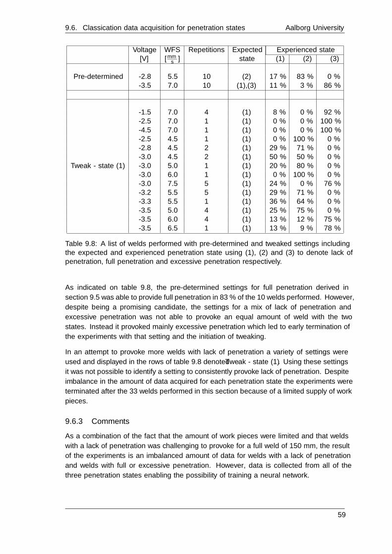
9.6. Classi�cation data acquisition for penetration states Aalborg University
Voltage WFS Repetitions Expected Experienced state[V] [mms ] state (1) (2) (3)
Pre-determined -2.8 5.5 10 (2) 17 % 83 % 0 %-3.5 7.0 10 (1),(3) 11 % 3 % 86 %
Tweak - state (1)
-1.5 7.0 4 (1) 8 % 0 % 92 %-2.5 7.0 1 (1) 0 % 0 % 100 %-4.5 7.0 1 (1) 0 % 0 % 100 %-2.5 4.5 1 (1) 0 % 100 % 0 %-2.8 4.5 2 (1) 29 % 71 % 0 %-3.0 4.5 2 (1) 50 % 50 % 0 %-3.0 5.0 1 (1) 20 % 80 % 0 %-3.0 6.0 1 (1) 0 % 100 % 0 %-3.0 7.5 5 (1) 24 % 0 % 76 %-3.2 5.5 5 (1) 29 % 71 % 0 %-3.3 5.5 1 (1) 36 % 64 % 0 %-3.5 5.0 4 (1) 25 % 75 % 0 %-3.5 6.0 4 (1) 13 % 12 % 75 %-3.5 6.5 1 (1) 13 % 9 % 78 %
Table 9.8: A list of welds performed with pre-determined and tweaked settings includingthe expected and experienced penetration state using (1), (2) and (3) to denote lack ofpenetration, full penetration and excessive penetration respectively.
As indicated on table 9.8, the pre-determined settings for full penetration derived in
section 9.5 was able to provide full penetration in 83 % of the 10 welds performed. However,
despite being a promising candidate, the settings for a mix of lack of penetration and
excessive penetration was not able to provoke an equal amount of weld with the two
states. Instead it provoked mainly excessive penetration which led to early termination of
the experiments with that setting and the initiation of tweaking.
In an attempt to provoke more welds with lack of penetration a variety of settings were
used and displayed in the rows of table 9.8 denoted Tweak - state (1). Using these settings
it was not possible to identify a setting to consistently provoke lack of penetration. Despite
imbalance in the amount of data acquired for each penetration state the experiments were
terminated after the 33 welds performed in this section because of a limited supply of work
pieces.
9.6.3 Comments
As a combination of the fact that the amount of work pieces were limited and that welds
with a lack of penetration was challenging to provoke for a full weld of 150 mm, the result
of the experiments is an imbalanced amount of data for welds with a lack of penetration
and welds with full or excessive penetration. However, data is collected from all of the
three penetration states enabling the possibility of training a neural network.
59

Anders Bidstrup 9. Experiment design and execution
9.7 Classi�cation data acquisition for transfer modes
The purpose of these experiments is to obtain data to be used in the classi�cation of the
transfer modes. Since a range of data for short-circuit transfer mode is obtained in the
classi�cation data acquisition for welding defects, see section 9.6, only data for globular
transfer is to be obtained in this range of experiments.
9.7.1 Speci�cation
For the simplest case of classifying the transfer modes only data from stable welds should
be used to provide a general guideline for the type of data the individual modes produce.
In the case of short-circuit transfer a stable setting turned out to be with a travel speed of
2 mms , a voltage adjustment of -2.8 V and a WFS adjustment of 5.5 m
min , see section 9.5
and section 9.6. In the identi�cation of penetration state and transfer mode settings, see
section 9.5, a stable weld for globular transfer was found when using a travel speed of 1mms , a voltage adjustment of 2 V and a WFS adjustment of -2 m
min . To obtain a suitable
amount of data for classi�cation, repetitive experiments using these settings should be
performed until the amount of data from the case of globular transfer roughly matches the
amount of data for short-circuit transfer, i.e. ≈ 10 repetitions of a 150 mm weld.
9.7.2 Results
Due to a machine breakdown the ABB robot was incapacitated and therefore did not allow
for the execution of further experiments.
9.7.3 Comments
Due to the machine breakdown of the ABB robot it was not possible to perform further
experiments. However, from the experiments of section 9.5 a small amount of data can
be extracted to use in the classi�cation. Although the data is sparse it could provide
knowledge as to whether classifying globular transfer and short-circuit transfer using sound
is feasible.
60

Data analysis 10As mentioned in chapter 6 the data acquired from the experiments in chapter 9 needs to
be preprocessed through labelling, removal of improper classi�cation data and �ltering. In
this chapter these steps are presented.
10.1 Data labelling
The labelling process is performed in two rounds - one for each hypothesis to test. Generally
one-hot encoding is used as speci�ed in appendix E to enable the use of cross-entropy.
10.1.1 Labelling of penetration states
As explained in section 9.5, three penetration states states exist:
[ 1 0 0 ] Lack of penetration
[ 0 1 0 ] Full penetration
[ 0 0 1 ] Excessive penetration
The labelling is done using Matlab. Initially the sound �le is imported and cut to only
include sound between the initial pulse of the weld to the �nal extinguishing pulse of the
weld. By doing so, a sound �le containing n amount of samples, equivalent to nFs seconds,
can be compared to the length of the weld in question. Afterwards it is determined how
much of the start and �nish of the weld should not be included due to the e�ect of the
tack weld. Through visual inspection and random sample comparison to ISO-5817, the
weld is then classi�ed in segments of constant penetration state after which each segment
is cut from the sound �le and given a label as indicated on �gure 10.1.
Figure 10.1: A weld segmented into three sections based on the penetration state.
61
Anders Bidstrup 10. Data analysis
Once this process is performed for all welds presented in section 9.6, merged sound �les
for each penetration state is made.
10.1.2 Labelling of transfer modes
As explained in section 9.7, two transfer modes are investigated:
[ 1 0 0 ] Globular transfer
[ 0 1 0 ] Short-circuit transfer
Due to the mechanical breakdown of the ABB robot, see section 9.7, a limited set of data
is used for globular transfer. Speci�cally only segments of two welds from the experiments
for identi�cation of penetration state and mode settings are assessed useful. In case of the
data for short-circuit transfer, the sound �le for full penetration extracted in the labelling
of the penetration states is used.
Since the transfer mode is constant for each full weld the labels are assigned to the full
sound �le. In the case for globular transfer, initially the sound �le is cut to include only
the sound of the weld excluding the start and �nish. Once this process is performed for
the two considered welds they are merged to one sound �le. In the case of short-circuit
transfer, the sound �le is simply relabelled.
10.2 Removal of improper classi�cation data
Since the merged sound �les consist of segments from welds performed at di�erent settings,
an amount of variance is expected in the data. Using this data trains the ANN to classify
despite of the variance which in turn makes it more �exible. However, the variance of
the data can be too excessive for the ANN to distinguish between the classes. Therefore
the merged sound �les are plotted and visually inspected for noticeable di�erence between
the segments from which they are merged. Should the data be assessed to cause more
confusion between classes than �exibility for the given class, the segment is removed from
the �le.
The amount of data removed due to the inspection results is shown in table 10.1.
Class Reduction of data [%]Lack of penetration 39Full penetration 2Globular transfer 0
Table 10.1: The reduction of data after removal of bad data from each penetration stateand globular transfer.
As speci�ed in table 10.1, the data from welds with lack of penetration had the largest
reduction of data with 39 %, whereas the data for the full penetration and globular transfer
su�ered a reduction of 2 % and 0 % respectively.
62
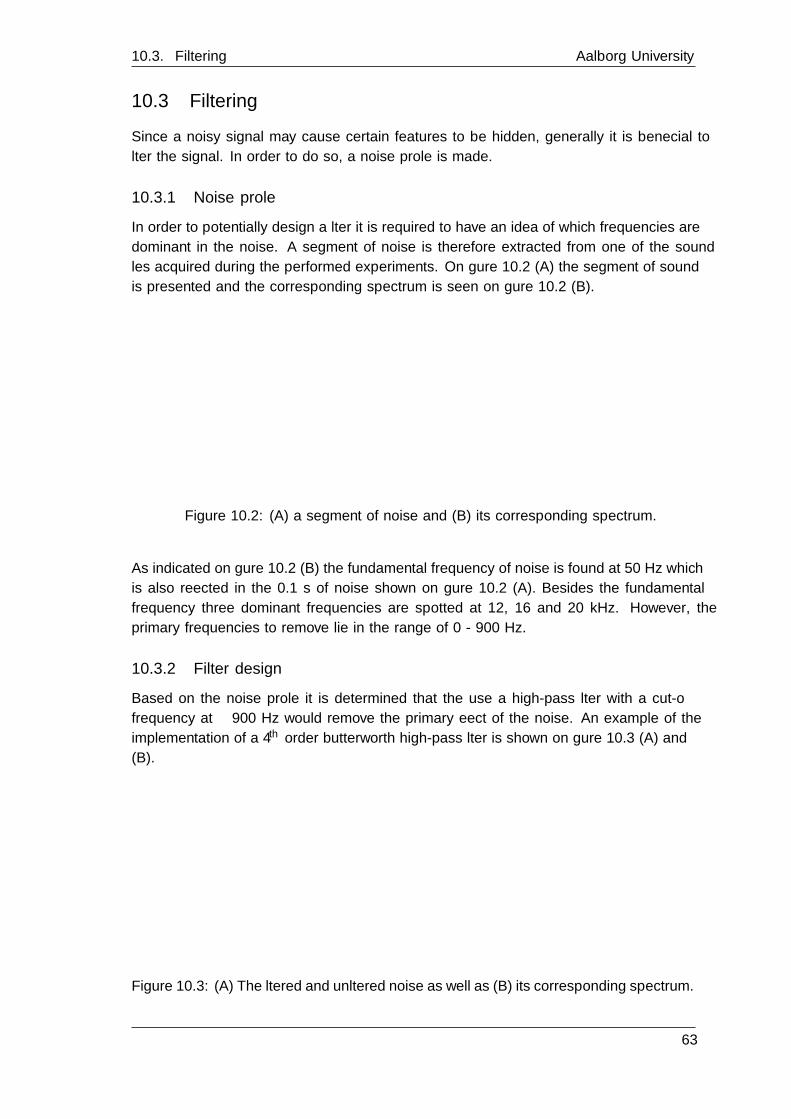
10.3. Filtering Aalborg University
10.3 Filtering
Since a noisy signal may cause certain features to be hidden, generally it is bene�cial to
�lter the signal. In order to do so, a noise pro�le is made.
10.3.1 Noise pro�le
In order to potentially design a �lter it is required to have an idea of which frequencies are
dominant in the noise. A segment of noise is therefore extracted from one of the sound
�les acquired during the performed experiments. On �gure 10.2 (A) the segment of sound
is presented and the corresponding spectrum is seen on �gure 10.2 (B).
0 0.02 0.04 0.06 0.08 0.1
Time [s]
-0.1
-0.05
0
0.05
0.1
Am
plitu
de
(A) Noise
0 5 10 15 20
Frequency (kHz)
-140
-120
-100
-80
-60
-40
Pow
er/fr
eque
ncy
(dB
/Hz)
(B) Welchs power spectral density
Fundamental frequency: 50 HzPeaks: 12, 16, 20 kHz
Figure 10.2: (A) a segment of noise and (B) its corresponding spectrum.
As indicated on �gure 10.2 (B) the fundamental frequency of noise is found at 50 Hz which
is also re�ected in the 0.1 s of noise shown on �gure 10.2 (A). Besides the fundamental
frequency three dominant frequencies are spotted at 12, 16 and 20 kHz. However, the
primary frequencies to remove lie in the range of 0 - 900 Hz.
10.3.2 Filter design
Based on the noise pro�le it is determined that the use a high-pass �lter with a cut-o�
frequency at ≈ 900 Hz would remove the primary e�ect of the noise. An example of the
implementation of a 4th order butterworth high-pass �lter is shown on �gure 10.3 (A) and
(B).
0 0.02 0.04 0.06 0.08 0.1
Time [s]
-0.06
-0.04
-0.02
0
0.02
0.04
0.06
Am
plitu
de
(A) Filtered vs unfiltered signal
Unfiltered signalFiltered signal
0 5 10 15 20
Frequency (kHz)
-140
-120
-100
-80
-60
-40
Pow
er/fr
eque
ncy
(dB
/Hz)
(B) Welchs power spectral density
Figure 10.3: (A) The �ltered and un�ltered noise as well as (B) its corresponding spectrum.
63

Anders Bidstrup 10. Data analysis
As shown on �gure 10.3 (A) the primary in�uence of the noise is eliminated. The spectrum
on �gure 10.3 (B) illustrates the consequence of the �ltering - frequencies below 900 Hz
are �ltered from the signal while the remaining spectrum is maintained.
10.3.3 Discussion
Applying a high-pass �lter with a cut-o� frequency of ≈ 900 Hz, e.g. a butterworth �lter,
eliminates the primary in�uence of the noise. However, since �ltering involves a loss of
information it is not necessarily bene�cial to perform. It is assessed that �ltering should
be avoided if possible but may be applied in an attempt to increase performance of the
ANN.
10.4 Feature extraction
In this section the discussion of which features to extract from the preprocessed data from
chapter 10 is presented alongside the complete list of features.
10.4.1 Feature choice discussion
As introduced in chapter 2 a range of temporal, spectral shape, harmonic and perceptual
features can be used to describe a signal. Especially the extraction of MFCCs as perceptual
features includes the interesting aspect of being well-known for its use in speech recognition,
which has been used for penetration state classi�cation in other reports, see chapter 4.
Furthermore, chapter 4 showed that using a wavelet packet decomposition, henceforth
WPD, made it possible to classify penetration state for GTAW based on acoustic emission.
Based on the two mentioned chapters it is decided to combine the methods to obtain a
rich feature space with features known to be useful in the classi�cation based on acoustic
signals.
10.4.2 List of features
The feature extraction is done in Matlab using primarily built-in functions. Should a
function for a given feature not be available, it will be manually coded or found from an
external source. The set of temporal, spectral shape, harmonic and perceptual features
alongside the code used to to extract them is shown in table 10.2.
64
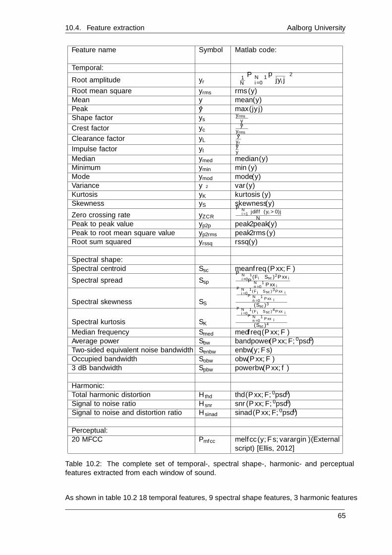
10.4. Feature extraction Aalborg University
Feature name Symbol Matlab code:
Temporal:
Root amplitude yr
(1N
∑N−1i=0
√|yi|)2
Root mean square yrms rms(y)Mean y mean(y)Peak y max(|y|)Shape factor ys
yrms
y
Crest factor ycy
yrms
Clearance factor yLyyr
Impulse factor yIyy
Median ymed median(y)Minimum ymin min(y)Mode ymod mode(y)Variance yσ2 var(y)Kurtosis yK kurtosis(y)Skewness yS skewness(y)
Zero crossing rate yZCR∑N
i=1 |diff(yi>0)|N
Peak to peak value yp2p peak2peak(y)Peak to root mean square value yp2rms peak2rms(y)Root sum squared yrssq rssq(y)
Spectral shape:
Spectral centroid Ssc meanfreq(Pxx, F )
Spectral spread Ssp
∑N−1i=0 (Fi−Ssc)2Pxxi∑N−1
n=0 Pxxi
Spectral skewness SS
∑N−1i=0
(Fi−Ssc)3Pxxi∑N−1
n=0 Pxxi
(Ssc)3
Spectral kurtosis SK
∑N−1i=0
(Fi−Ssc)4Pxxi∑N−1
n=0 Pxxi
(Ssc)4
Median frequency Smed medfreq(Pxx, F )Average power Sbw bandpower(Pxx, F,′ psd′)Two-sided equivalent noise bandwidth Senbw enbw(y, Fs)Occupied bandwidth Sobw obw(Pxx, F )3 dB bandwidth Spbw powerbw(Pxx, f)
Harmonic:
Total harmonic distortion Hthd thd(Pxx, F,′ psd′)Signal to noise ratio Hsnr snr(Pxx, F,′ psd′)Signal to noise and distortion ratio Hsinad sinad(Pxx, F,′ psd′)
Perceptual:
20 MFCC Pmfcc melfcc(y, Fs, varargin)(Externalscript) [Ellis, 2012]
Table 10.2: The complete set of temporal-, spectral shape-, harmonic- and perceptualfeatures extracted from each window of sound.
As shown in table 10.2 18 temporal features, 9 spectral shape features, 3 harmonic features
65
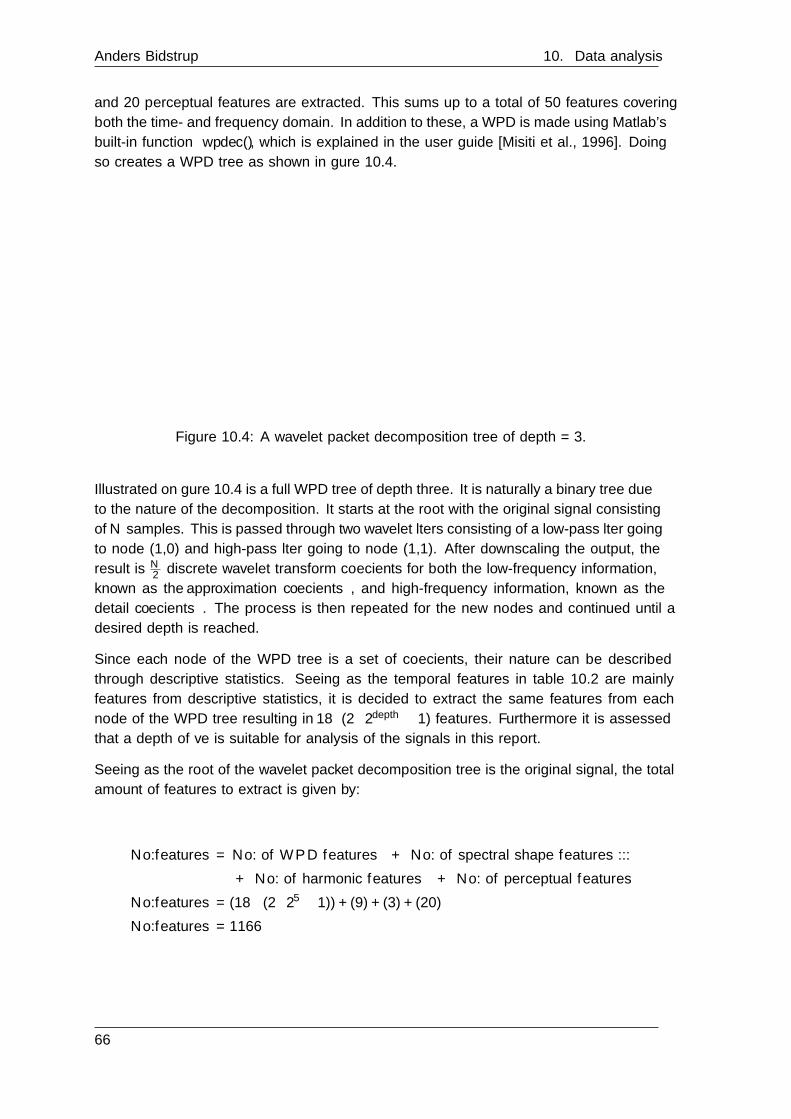
Anders Bidstrup 10. Data analysis
and 20 perceptual features are extracted. This sums up to a total of 50 features covering
both the time- and frequency domain. In addition to these, a WPD is made using Matlab's
built-in function wpdec(), which is explained in the user guide [Misiti et al., 1996]. Doing
so creates a WPD tree as shown in �gure 10.4.
Figure 10.4: A wavelet packet decomposition tree of depth = 3.
Illustrated on �gure 10.4 is a full WPD tree of depth three. It is naturally a binary tree due
to the nature of the decomposition. It starts at the root with the original signal consisting
of N samples. This is passed through two wavelet �lters consisting of a low-pass �lter going
to node (1,0) and high-pass �lter going to node (1,1). After downscaling the output, the
result is N2 discrete wavelet transform coe�cients for both the low-frequency information,
known as the approximation coe�cients, and high-frequency information, known as the
detail coe�cients. The process is then repeated for the new nodes and continued until a
desired depth is reached.
Since each node of the WPD tree is a set of coe�cients, their nature can be described
through descriptive statistics. Seeing as the temporal features in table 10.2 are mainly
features from descriptive statistics, it is decided to extract the same features from each
node of the WPD tree resulting in 18 · (2 · 2depth − 1) features. Furthermore it is assessed
that a depth of �ve is suitable for analysis of the signals in this report.
Seeing as the root of the wavelet packet decomposition tree is the original signal, the total
amount of features to extract is given by:
No.features = No. of WPD features + No. of spectral shape features ...
+ No. of harmonic features + No. of perceptual features
No.features = (18 · (2 · 25 − 1)) + (9) + (3) + (20)
No.features = 1166
66

Model training andperformance evaluation 11
In this chapter a range of neural networks are trained with the aim of providing evidence
to either accept or reject the hypotheses listed in chapter 5. Initially the challenges of
designing the network and handling the data is discussed along with a description of the
program used to execute the procedure. The results are then presented and commented
on individually for the two sub-hypotheses.
11.1 Procedure
Before training a neural network, a range of decisions must be made:
� Should the signal be �ltered?
� What window type, window size and overlap should be used?
� Should feature scaling be performed?
� Should dimensionality reduction be performed?
� What should the con�guration of the network be?
� What optimisation method should be used?
The grounds for each decision is presented individually including an explanation of the
�nal program made to execute the developed procedure.
11.1.1 Filtering
Based on the information presented in section 10.3, it is decided not to �lter the signal
to preserve as much information about the signal as possible. To obtain an idea of the
impact of this decision initial experiments were made with various high-pass �lters which
showed little to no change in the accuracy of the trained models.
11.1.2 Window type, window size and overlap
The window size and overlap play an important role in the balancing of data set size and
information per segment when working with limited data, see chapter 2. Furthermore the
type of window determines where the weight of the window should be, see chapter 2. The
e�ect of each and the decision made is presented individually.
67

Anders Bidstrup 11. Model training and performance evaluation
Window type
Using a non-constant window such as the Hamming window, see chapter 2, subjects the
values in the window to a variable gain, hereby putting more or less focus on parts of the
window. While this can cause a potential bene�t, it is decided to use of a rectangular, i.e.
constant, window for the testing of the hypotheses in this report.
Window size
When determining the size of the window to use, one should analyse the signal to ensure
that at least one repetition of the expected behaviour is performed. However, under
the assumption that a state is constant for the duration of the window, an increased
windows size causes an averaging e�ect over multiple repetitions which counteracts the
variance between individual repetitions. Although providing a possible bene�t in terms of
averaging, doing so results in fewer windows for a given length of signal which potentially
has a negative e�ect on the performance of the trained model by not capturing enough
variance to properly classify the data.
Based on the uncertainty of the choice, it is determined to investigate the cases of using a
window size of either 0.25 s, 0.50 s, 1.00 s, 2.00 s and 4.00 s. Using this range of window
sizes is assessed to produce indications of the e�ect of increasing and decreasing window
size and provide a guideline for future projects.
Overlap
As explained in chapter 2, using an overlap also creates an averaging e�ect on the features
extracted from the signal. Furthermore, when using a limited data set, more windows can
be extracted from the signal depending on the length of the signal and the size of the
overlap. However, since the averaging e�ect is in the transition from a previous window
to the current, it is unclear whether the use of the overlap has a bene�cial e�ect on the
performance of the ANN or if the repetition of the same data yields no improvement.
Based on the uncertainty of the choice, it is determined to investigate the cases of using
an overlap of either 0 %, 25 % or 50 % on each case of window size.
11.1.3 Feature scaling
As presented in chapter 3, feature scaling can yield a bene�cial e�ect on the performance
of the ANN. It is therefore decided to include feature scaling.
11.1.4 Dimensionality reduction
Having 1166 features in total, see chapter 10, the use of dimensionality reduction might
prove to be bene�cial for the performance of the algorithm. However, before investigating
the e�ect of dimensionality reduction, it is decided to train the ANNs on the full set of
features.
68

11.1. Procedure Aalborg University
11.1.5 Network con�guration
The term Network con�guration is in this report used to denote the structure of the
ANN, i.e. the amount of hidden layers and neurons in each layer. Since the best network
con�guration is unknown it is decided to investigate a range of possibilities, see chapter 7.
Speci�cally it is decided to consider the network having either one or two layers each
consisting of 5-15 neurons. It is assessed that using this range of neurons and layers gives
general insight as to which con�guration is desired in the classi�cation cases of this project.
11.1.6 Optimisation method
Based on the information presented in chapter 3 and chapter 7, it is decided to investigate
the use of both GDA and SCG. The decision of using GDA lies in the use of adaptive
learning rate, which improves the convergence rate of the optimisation compared to GD.
In addition to this characteristic, the SCG is supposedly better at handling non-convex
problems and allows faster convergence based on non-orthogonal steps and use of second-
order information.
11.1.7 Program
To analyse the performance of the ANN model based on the decisions made in section 11.1,
a Matlab program is made to cycle through all combinations. The general procedure is
shown in a tree representation on �gure 11.1.
69

Anders Bidstrup 11. Model training and performance evaluation
Figure 11.1: A tree representation of the program used to window a signal, extract featuresfrom the windows and train a range of ANNs.
To ease the explanation of the procedure only one branch of the tree is shown on �gure 11.1.
As shown, the sound �le, is initially windowed using a window size of either 0.25 s, 0.50 s,
1.00 s, 2.00 s or 4.00 s and an overlap of either 0 %, 25 % or 50 %. Once the windowing
is done, the features are extracted, feature scaled and sent to loop through ANN training
with the speci�ed network con�guration.
For the network generation and training the Neural Network Toolbox of Matlab is used.
The following settings are set for GDA:
� Initial learning rate: 0.5
� Maximum cost increase: 1.04
� Ratio to increase learning rate: 1.05
70

11.2. Results Aalborg University
� Ratio to decrease learning rate: 0.7
For SCG two constants need to be de�ned:
� Change in weight for second derivative approximation: 5.0 · 10−5
� Parameter for regulating the inde�niteness of the Hessian: 5.0 · 10−7
Lastly training termination occurs if:
� ... 1000 iterations is reached
� ... the gradient reaches 1 · 10−5
� ... 6 consecutive cost increases is experienced
� ... the performance goal of 0 is reached.
For a commented version of the entire Matlab program and used functions, see enclosure
B.
11.2 Results
After running the program for both the penetration state classi�cation and transfer
mode classi�cation, information about the network con�guration with the best test
set performance is extracted and presented individually. Throughout this section the
terminology presented in table 11.1 is used.
Abbreviation Full namewsize Window sizewo OverlapN1 No. of data points for class 1N2 No. of data points for class 2N3 No. of data points for class 3Nall No. of data points in totalGDA Gradient descent with adaptive learning rateSCG Scaled conjugate gradient descentFS Feature scalingPCA Principle component analysisBC Best con�gurationACC Accuracy
Table 11.1: A list of abbreviations and their full names.
11.2.1 Penetration state classi�cation
In order to gather evidence to either accept or reject h1.1 from chapter 5, the program
presented in section 11.1 is run on the data collected in the classi�cation data acquisition
for penetration states, see section 9.6, after performing the preprocessing described in
chapter 10. The result is shown in table 11.2.
71
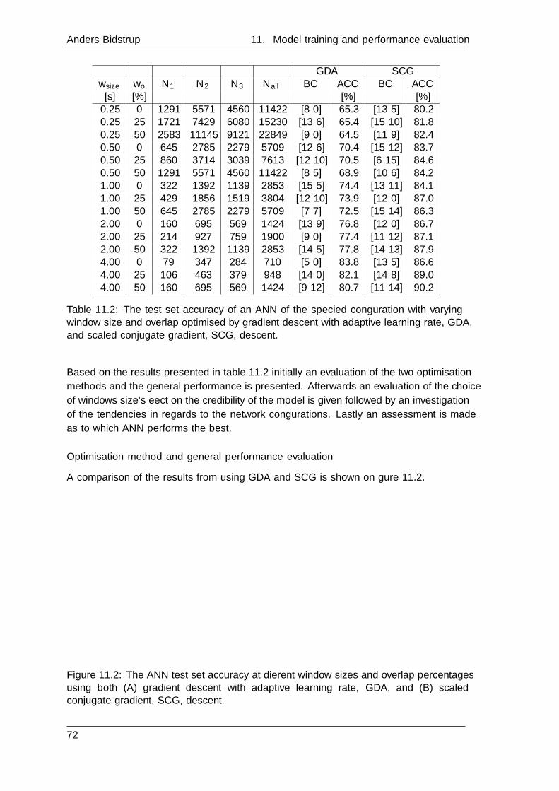
Anders Bidstrup 11. Model training and performance evaluation
GDA SCGwsize wo N1 N2 N3 Nall BC ACC BC ACC
[s] [%] [%] [%]0.25 0 1291 5571 4560 11422 [8 0] 65.3 [13 5] 80.20.25 25 1721 7429 6080 15230 [13 6] 65.4 [15 10] 81.80.25 50 2583 11145 9121 22849 [9 0] 64.5 [11 9] 82.40.50 0 645 2785 2279 5709 [12 6] 70.4 [15 12] 83.70.50 25 860 3714 3039 7613 [12 10] 70.5 [6 15] 84.60.50 50 1291 5571 4560 11422 [8 5] 68.9 [10 6] 84.21.00 0 322 1392 1139 2853 [15 5] 74.4 [13 11] 84.11.00 25 429 1856 1519 3804 [12 10] 73.9 [12 0] 87.01.00 50 645 2785 2279 5709 [7 7] 72.5 [15 14] 86.32.00 0 160 695 569 1424 [13 9] 76.8 [12 0] 86.72.00 25 214 927 759 1900 [9 0] 77.4 [11 12] 87.12.00 50 322 1392 1139 2853 [14 5] 77.8 [14 13] 87.94.00 0 79 347 284 710 [5 0] 83.8 [13 5] 86.64.00 25 106 463 379 948 [14 0] 82.1 [14 8] 89.04.00 50 160 695 569 1424 [9 12] 80.7 [11 14] 90.2
Table 11.2: The test set accuracy of an ANN of the speci�ed con�guration with varyingwindow size and overlap optimised by gradient descent with adaptive learning rate, GDA,and scaled conjugate gradient, SCG, descent.
Based on the results presented in table 11.2 initially an evaluation of the two optimisation
methods and the general performance is presented. Afterwards an evaluation of the choice
of windows size's e�ect on the credibility of the model is given followed by an investigation
of the tendencies in regards to the network con�gurations. Lastly an assessment is made
as to which ANN performs the best.
Optimisation method and general performance evaluation
A comparison of the results from using GDA and SCG is shown on �gure 11.2.
0.25 0.50 1.00 2.00 4.00
Window size [s]
65
70
75
80
85
90
95
100
Acc
urac
y [%
]
(A) GDA ANN test set accuracy
0 % Overlap25 % Overlap50 % Overlap
0.25 0.50 1.00 2.00 4.00
Window size [s]
65
70
75
80
85
90
95
100
Acc
urac
y [%
]
(B) SCG ANN test set accuracy
0 % Overlap25 % Overlap50 % Overlap
Figure 11.2: The ANN test set accuracy at di�erent window sizes and overlap percentagesusing both (A) gradient descent with adaptive learning rate, GDA, and (B) scaledconjugate gradient, SCG, descent.
72
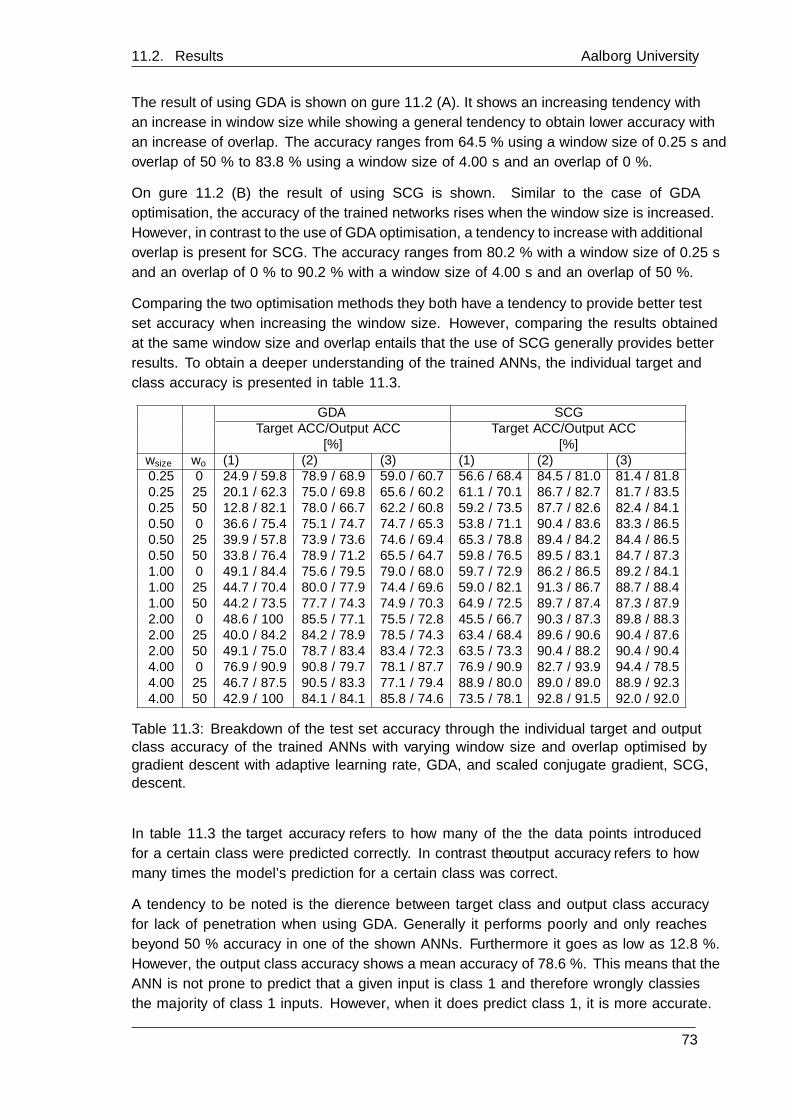
11.2. Results Aalborg University
The result of using GDA is shown on �gure 11.2 (A). It shows an increasing tendency with
an increase in window size while showing a general tendency to obtain lower accuracy with
an increase of overlap. The accuracy ranges from 64.5 % using a window size of 0.25 s and
overlap of 50 % to 83.8 % using a window size of 4.00 s and an overlap of 0 %.
On �gure 11.2 (B) the result of using SCG is shown. Similar to the case of GDA
optimisation, the accuracy of the trained networks rises when the window size is increased.
However, in contrast to the use of GDA optimisation, a tendency to increase with additional
overlap is present for SCG. The accuracy ranges from 80.2 % with a window size of 0.25 s
and an overlap of 0 % to 90.2 % with a window size of 4.00 s and an overlap of 50 %.
Comparing the two optimisation methods they both have a tendency to provide better test
set accuracy when increasing the window size. However, comparing the results obtained
at the same window size and overlap entails that the use of SCG generally provides better
results. To obtain a deeper understanding of the trained ANNs, the individual target and
class accuracy is presented in table 11.3.
GDA SCGTarget ACC/Output ACC Target ACC/Output ACC
[%] [%]wsize wo (1) (2) (3) (1) (2) (3)0.25 0 24.9 / 59.8 78.9 / 68.9 59.0 / 60.7 56.6 / 68.4 84.5 / 81.0 81.4 / 81.80.25 25 20.1 / 62.3 75.0 / 69.8 65.6 / 60.2 61.1 / 70.1 86.7 / 82.7 81.7 / 83.50.25 50 12.8 / 82.1 78.0 / 66.7 62.2 / 60.8 59.2 / 73.5 87.7 / 82.6 82.4 / 84.10.50 0 36.6 / 75.4 75.1 / 74.7 74.7 / 65.3 53.8 / 71.1 90.4 / 83.6 83.3 / 86.50.50 25 39.9 / 57.8 73.9 / 73.6 74.6 / 69.4 65.3 / 78.8 89.4 / 84.2 84.4 / 86.50.50 50 33.8 / 76.4 78.9 / 71.2 65.5 / 64.7 59.8 / 76.5 89.5 / 83.1 84.7 / 87.31.00 0 49.1 / 84.4 75.6 / 79.5 79.0 / 68.0 59.7 / 72.9 86.2 / 86.5 89.2 / 84.11.00 25 44.7 / 70.4 80.0 / 77.9 74.4 / 69.6 59.0 / 82.1 91.3 / 86.7 88.7 / 88.41.00 50 44.2 / 73.5 77.7 / 74.3 74.9 / 70.3 64.9 / 72.5 89.7 / 87.4 87.3 / 87.92.00 0 48.6 / 100 85.5 / 77.1 75.5 / 72.8 45.5 / 66.7 90.3 / 87.3 89.8 / 88.32.00 25 40.0 / 84.2 84.2 / 78.9 78.5 / 74.3 63.4 / 68.4 89.6 / 90.6 90.4 / 87.62.00 50 49.1 / 75.0 78.7 / 83.4 83.4 / 72.3 63.5 / 73.3 90.4 / 88.2 90.4 / 90.44.00 0 76.9 / 90.9 90.8 / 79.7 78.1 / 87.7 76.9 / 90.9 82.7 / 93.9 94.4 / 78.54.00 25 46.7 / 87.5 90.5 / 83.3 77.1 / 79.4 88.9 / 80.0 89.0 / 89.0 88.9 / 92.34.00 50 42.9 / 100 84.1 / 84.1 85.8 / 74.6 73.5 / 78.1 92.8 / 91.5 92.0 / 92.0
Table 11.3: Breakdown of the test set accuracy through the individual target and outputclass accuracy of the trained ANNs with varying window size and overlap optimised bygradient descent with adaptive learning rate, GDA, and scaled conjugate gradient, SCG,descent.
In table 11.3 the target accuracy refers to how many of the the data points introduced
for a certain class were predicted correctly. In contrast the output accuracy refers to how
many times the model's prediction for a certain class was correct.
A tendency to be noted is the di�erence between target class and output class accuracy
for lack of penetration when using GDA. Generally it performs poorly and only reaches
beyond 50 % accuracy in one of the shown ANNs. Furthermore it goes as low as 12.8 %.
However, the output class accuracy shows a mean accuracy of 78.6 %. This means that the
ANN is not prone to predict that a given input is class 1 and therefore wrongly classi�es
the majority of class 1 inputs. However, when it does predict class 1, it is more accurate.
73

Anders Bidstrup 11. Model training and performance evaluation
Considering the target class and output class accuracy of the remaining two classes, the
model performs better than for class 1 with higher target class accuracy and a smaller gap
between target class accuracy and output class accuracy.
In the case of the ANNs trained with SCG, the results are generally better. The same
tendency of having a lower target class and output class accuracy for class 1 compared to
class 2 and 3 is also found for these ANNs. However, the gap between the target class
accuracy and output accuracy for class 1 is smaller than for the ANNs trained using GDA.
Furthermore, the general accuracy for the ANNs trained using SCG is better than for those
trained using GDA.
Window size and overlap evaluation
Based on the data presented in table 11.2 the e�ect of averaging with increased window size
explained in section 11.1 seems to yield an improvement of the performance of the networks.
In the case of increasing overlap only the ANNs trained on SCG seem to experience a
stable improvement, while cases of increases and decreases in the accuracy of the ANN is
experienced using GDA. In regards to the window size, it should be noted that the e�ect
on the size of the data set lowers the credibility of the result. To illustrate the reduction,
�gure 11.3 shows the total amount of data points extracted from the signal based on the
window size and overlap.
Number of overall samples
0.25 0.50 1.00 2.00 4.00
Window size [s]
0
0.5
1
1.5
2
2.5
Sam
ples
104
0 % Overlap25 % Overlap50 % Overlap
Figure 11.3: The number of samples as a function of the window size and overlappercentage.
As seen on �gure 11.3 the amount of data points is halved with a doubling of the window
size. With the limited data set used in this project this decrease can result in insu�cient
training data and in turn poor �exibility when introduced to new data, i.e. being over�tted.
With an increase of overlap it is possible to obtain more windows per data set which could
explain the increase in test set accuracy due to overlap experienced for the ANNs trained
using SCG.
Network con�guration tendency evaluation
As indicated in table 11.2 the best network con�guration for the majority of the
combinations consists of two layers. To obtain a general idea of how many neurons to
place in each layer in this case, the distribution of neurons in the two layers for the best
con�gurations is shown on �gure 11.4.
74
11.2. Results Aalborg University
5 10 15
Neurons in layer 1
0
1
2
3
4
5
6
Obs
erva
tions
(A) Neurons in layer 1
5 10 15
Neurons in layer 2
0
1
2
3
4
5
6
Obs
erva
tions
(B) Neurons in layer 2
Figure 11.4: The distribution of neurons in the cases where two layers are used.
As indicated by �gure 11.4 (A), the distribution of neurons in the �rst layer shows a mode
of 13 neurons and a mean of 12.0 neurons. In relation to the second layer, the distribution
on �gure 11.4 (B) shows a mode of 5 neurons with a mean of 9.1 neurons. Furthermore
the di�erence in neurons from the �rst to the second layer yields a tendency to have fewer
neurons in the second layer. The mean di�erence is calculated to 2.9 neurons with a mode
of 2 neurons.
In the case of having one layer the mode is 9 neurons and shows a mean of 9.9 neurons.
Best performance evaluation
Determining the overall best ANN based on the overall accuracy of the network as presented
in table 11.2 may result in a network with poor performance when classifying class 1.
Therefore the decision is also based on the target class and output class accuracy measures
leading to the conclusion that the ANN trained using SCG based on features from windows
of 4.00 s with an overlap of 25 % is the best of the trained ANNs. This network shows
target class accuracy measures of 88.9 %, 89.0 % and 88.9 % and corresponding output
class accuracy measures of 80.0 %, 89.0 % and 92.3 % for class 1, class 2 and class 3
respectively resulting in an overall accuracy of 89.0 %.
11.2.2 Transfer mode classi�cation
In order to gather evidence to either accept or reject h1.2 from chapter 5, the program
presented in section 11.1 is run on the acquired data for globular transfer and an
equal amount of data for short-circuit transfer from the classi�cation data acquisition
for penetration state, see section 9.7, after performing the preprocessing described in
chapter 10. A tendency to have an accuracy of 100 % regardless of network con�guration
was discovered during initial experiments. Based on this the program was simpli�ed to
only train networks of one layer with 10 neurons. The results are shown in table 11.4.
75
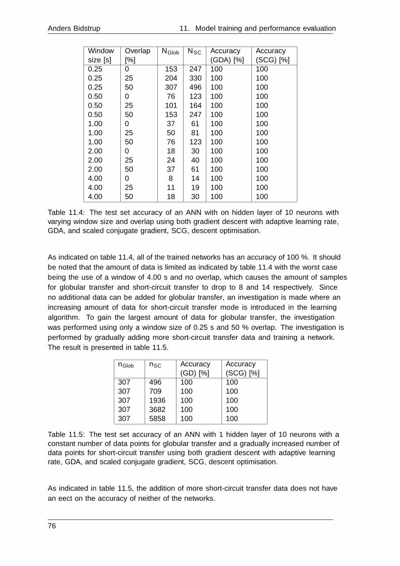
Anders Bidstrup 11. Model training and performance evaluation
Windowsize [s]
Overlap[%]
NGlob NSC Accuracy(GDA) [%]
Accuracy(SCG) [%]
0.25 0 153 247 100 1000.25 25 204 330 100 1000.25 50 307 496 100 1000.50 0 76 123 100 1000.50 25 101 164 100 1000.50 50 153 247 100 1001.00 0 37 61 100 1001.00 25 50 81 100 1001.00 50 76 123 100 1002.00 0 18 30 100 1002.00 25 24 40 100 1002.00 50 37 61 100 1004.00 0 8 14 100 1004.00 25 11 19 100 1004.00 50 18 30 100 100
Table 11.4: The test set accuracy of an ANN with on hidden layer of 10 neurons withvarying window size and overlap using both gradient descent with adaptive learning rate,GDA, and scaled conjugate gradient, SCG, descent optimisation.
As indicated on table 11.4, all of the trained networks has an accuracy of 100 %. It should
be noted that the amount of data is limited as indicated by table 11.4 with the worst case
being the use of a window of 4.00 s and no overlap, which causes the amount of samples
for globular transfer and short-circuit transfer to drop to 8 and 14 respectively. Since
no additional data can be added for globular transfer, an investigation is made where an
increasing amount of data for short-circuit transfer mode is introduced in the learning
algorithm. To gain the largest amount of data for globular transfer, the investigation
was performed using only a window size of 0.25 s and 50 % overlap. The investigation is
performed by gradually adding more short-circuit transfer data and training a network.
The result is presented in table 11.5.
nGlob nSC Accuracy(GD) [%]
Accuracy(SCG) [%]
307 496 100 100307 709 100 100307 1936 100 100307 3682 100 100307 5858 100 100
Table 11.5: The test set accuracy of an ANN with 1 hidden layer of 10 neurons with aconstant number of data points for globular transfer and a gradually increased number ofdata points for short-circuit transfer using both gradient descent with adaptive learningrate, GDA, and scaled conjugate gradient, SCG, descent optimisation.
As indicated in table 11.5, the addition of more short-circuit transfer data does not have
an e�ect on the accuracy of neither of the networks.
76

Discussion 12Based on the results from the classi�cation of penetration state and transfer mode a
discussion is made to argue whether su�cient evidence is present to accept the hypotheses
presented in chapter 5. An individual discussion for each sub-hypothesis is presented in
this section.
h1.1: It is possible to identify the penetration state of GMAW through its acoustic
emission using an arti�cial neural network
A range of networks was trained through both gradient descent with adaptive learning
rate, GDA, and scaled conjugate gradient, SCG, descent using a total of 1166 features
from rectangular windows of 0.25 s, 0.50 s, 1.00 s, 2.00 or 4.00 s with an overlap of 0 %,
25 % or 50 %. The results showed a tendency for increased accuracy for ANNs trained
through GDA and SCG with increased window size as expected from the averaging e�ect
it has. Furthermore the use of overlapping yielded bene�cial results in terms of accuracy
for ANNs traing through SCG while both increases and decreases are experienced for
ANNs trained through GDA. The accuracy is expected to increase based on the averaging
e�ect of larger windows as well as overlapping which is true for the case of ANNs trained
through SCG. Since a contradictory result is found for the ANNs trained through GDA, it
is plausible that the choice of optimisation method is to blame. From the investigation of
the target class and output class accuracy measures it is derived that the target accuracy
for the ANNs trained through GDA primarily lies below 50 %. This suggests the model
being biased towards class 2 and 3, possibly due to the imbalance of data or wrong choice
of features. However, based on the fact that ANNs trained through SCG do not have this
problem and are able to produce target class and output class accuracy measures of 80 %
and above, it is assessed that the problem lies with the optimisation method. A reason for
this may be GDA's challenge of handling non-convexity.
Since target class and output class accuracy measures for class 2 and 3 for the ANNs
trained through GDA are consistently greater than 70 % when using a window size of 2.00
s or 4.00 s regardless of overlap it is assessed that there is not enough evidence to reject
h1.1 for these cases. However, based on the consistently low target class accuracy for class
1, it is assessed that there is enough evidence to reject the hypothesis for these cases.
In regards to the ANNs trained through SCG it is assessed that there is not enough
evidence to reject h1.1 for any of the classes when using either a window size of 2.00 s with
an overlap of 25 % or 50 % or a window size of 4.00 s regardless of overlap.
h1.2: It is possible to identify the metal transfer mode of GMAW through its acoustic
emission using an arti�cial neural network
77

Anders Bidstrup 12. Discussion
In the case of classi�cation of transfer mode, the same program as for the classi�cation
of penetration state was used. However, in this case the trained ANNs all consist of one
hidden layer with 10 neurons based on early indications of producing models with 100 %
overall accuracy regardless of network con�guration. The results show that the trained
ANNs all have 100 % accuracy regardless of window size, overlap and optimisation method.
This is possibly the result of the lack of data present in the classi�cation. The lack of data
is illustrated in the data sets reaching a total of 22 data points for the worst case. However,
the lack of data is also caused by the total data set for globular transfer only being based
on two separate welds. Because of this only a small amount of variance is experienced
which causes the model to be over�tted to the presented data and a poor performance on
newly introduced data is expected. However, based on the fact that all the trained ANNs
has an accuracy of 100 % it is assessed that there is not enough evidence to reject h1.2.
78
Conclusion 13The purpose of this report was to investigate the acoustic response of GMAW's capabilities
in machine learning-based weld quality monitoring. To do so, an understanding of welding
theory, signal theory and machine learning was built. In combination with a study of
related work, a research area was speci�ed through the following hypothesis and sub-
hypotheses:
h1: It is possible to monitor GMAW using an arti�cial neural network trained on
labelled acoustic data
h1.1: It is possible to identify the penetration state of GMAW through its acous-
tic emission using an arti�cial neural network
h1.2: It is possible to identify the metal transfer mode of GMAW through its
acoustic emission using an arti�cial neural network
In order to test the hypotheses a robot cell capable of performing GMAW was modi�ed
so that voltage, current and sound from the process could be acquired. Experiments
were performed to acquire data from three penetration states - lack of penetration, full
penetration and excessive penetration - and two transfer modes - globular transfer and
short-circuit transfer. The sound �les were then windowed and labelled according to
penetration state and transfer mode using one-hot encoding. In order to investigate the
e�ect of window size, overlap, optimisation method and network con�guration, a Matlab
program was developed to run through every combination of a range of a range of window
sizes and overlaps as well as 110 di�erent ANN con�gurations. Furthermore the ANNs were
trained through gradient descent with adaptive learning rate, GDA, and scaled conjugate
gradient, SCG, descent. For each combination of window size and overlap, 1166 features
were extracted consisting of 18 temporal features, 9 spectral shape features, 3 harmonic
features, 20 perceptual features and 18 features from descriptive statistics for each node
of a 5-level wavelet packet decomposition with a db4 mother wavelet.
Using the described method it was possible to train an ANN with target class accuracy
of 88.9 %, 89.0 % and 88.9 % and corresponding output class accuracy of 80.0 %, 89 %
and 92.3 % for the three penetration states respectively resulting in an overall accuracy
of 89.0 %. Furthermore it was possible to train ANNs of 100 % overall accuracy in the
classi�cation of transfer mode.
Based on the �ndings of this project it is assessed that there is not enough evidence to
reject the hypothesis, h1, based on the following assessments for hypothesis h1.1 and h1.2.
79

Anders Bidstrup 13. Conclusion
h1.1: It is possible to identify the penetration state of GMAW through its acoustic
emission using an arti�cial neural network
Based on the results of the classi�cation of penetration states it is assessed that not enough
evidence is present to reject the hypothesis for ANNs trained through SCG using features
from windows of 2.00 s with an overlap of 25 % or 50 % or windows of 4.00 s using an
overlap of either 0 %, 25 % or 50 %. Furthermore, it is assessed that there is not enough
evidence present to reject the hypothesis for classi�cation of full penetration and excessive
penetration for ANNs trained through GDA using features from windows of 2.00 s or 4.00
s regardless of having an overlap of 0 %, 25 % or 50 %. Lastly it is assessed that enough
evidence is present to reject the hypothesis for classifying lack of penetration in the case
investigated in this project for ANNs trained through GDA regardless of using a window
size of 0.25 s, 0.50 s, 1.00 s, 2.00 s, 4.00 s with an overlap of 0 %, 25 % or 50 %.
h1.2: It is possible to identify the metal transfer mode of GMAW through its acoustic
emission using an arti�cial neural network
Based on the results of the classi�cation of transfer mode it is assessed that not enough
evidence is present to reject the hypothesis for any combination of window size, overlap
and optimisation method investigated in this project.
80

Perspectives 14Based on the decisions made and consequent �ndings of this report, a range of perspectives
and ideas for future work is derived and presented in this chapter.
14.1 Perspectives
The following perspectives are presented:
� Reduction of process variance
� Acquisition of more data
� Investigation general performance
� Noise reduction
� Reduction of feature space
� Expansion of feature space
� Inclusion of voltage and current features
� Inclusion of seam geometry features
� Inclusion of molten pool monitoring
� Inclusion of more transfer mode classes
� Alternative optimisation methods
� Alternative supervised classi�ers
� Use of regression
� Use of reinforcement learning
� Implement online monitoring
� Implement control
To specify, each of the listed perspectives are discussed individually.
Reduction of process variance
The experienced variance due to the process nature and setup limitations in this project
caused problems in consistent penetration state provoking. By reducing the variance the
quality of the acquired data could be improved and potentially improve the accuracy of
the trained classi�er.
Acquisition of more data
To increase the credibility of the trained models, more data for the cases of short-circuit
lack of penetration and globular transfer mode could be collected.
81

Anders Bidstrup 14. Perspectives
Investigation of general performance
Since the classi�ers of this report was trained on data for a speci�c case of short-circuit
GMAW of �at square grooved butt welds in steel with a 2 mm gap using a 1.2 mm rutile
�ux-cored wire using constant control variables, it could be interesting to investigate the
trained ANNs' accuracy when introduced to new cases or train new models to accommodate
for the introduced changes.
Noise reduction
The acquired sound showed a signi�cant amount of sound which was only brie�y
investigated. A thorough investigation of the noise pro�le and the use of �ltering could
be done to reduce its potential e�ect on the model. Furthermore, to make the model
suitable for implementation in industry, a study on the sensitivity of the method could
be performed possibly involving the implementation of more microphones and use of the
Cocktail-party algorithm.
Reduction of feature space
Through this project it was not attempted to reduce the feature space. As a consequence
of this, no insight as to which features are dominating is derived and the feature
space may include redundancies. To keep simple feature interpretation methods such
as forward feature construction or backwards feature elimination could be used. If feature
interpretability is less important, the use principle component analysis could be used.
Expansion of feature space
Although 1166 features were extracted from every window in case of this report, the list
of possible features is endless. Including more features may improve the accuracy of the
models if the new features are better at discriminating between the investigated classes.
Inclusion of voltage and current features
Since it was concluded in chapter 4 that the sound is highly related to the arc stability,
using information from the current and voltage measurements may prove bene�cial for the
accuracy of the model.
Inclusion of seam geometry features
Although the goal of this project was to investigate the acoustic response of GMAW's
capability within machine learning-based quality monitoring, it may increase general
performance of the model to be trained on features describing the seam geometry.
Inclusion of molten pool monitoring
Including monitoring of the molten weld pool may provide information relevant for the
penetration status and transfer mode of the process.
82

14.1. Perspectives Aalborg University
Inclusion of more transfer mode classes
In the case of this report, only globular transfer and short-circuit transfer was investigated.
However, more metal transfer modes could be included in the classi�cation such as spray
transfer and pulsed spray transfer, which would further generalise the model.
Alternative optimisation methods
Only gradient descent with adaptive learning rate and scaled conjugate gradient descent
was investigated in this report. However, the use of other optimisation methods may prove
to have a positive e�ect on the accuracy of the ANNs and their training convergence rate.
Alternative supervised classi�ers
In this report it was decided to investigate ANNs. However, a wide range of other
supervised classi�ers exist which may improve the accuracy of the prediction. Examples
could be the use of decision trees as introduced in chapter 4 or instance-based algorithms.
Use of regression
Besides alternative supervised classi�ers, the use of regression could be investigated.
Mapping a continuous function to the sound features would ease the process of developing
a closed loop system able of e.g. securing the correct penetration state.
Use of reinforcement learning
Another interesting direction is investigating the use of reinforcement learning. When
introduced to a new material or joint design it is possibly required to determine new
settings for the process. Reinforcement learning could be applied to develop a versatile,
automated process to handle this aspect through a �tness function based on e.g. the seam
geometry.
Implement online monitoring
Since the current models are performed post-weld, it could be bene�cial to implement the
model for online monitoring. Doing this also opens up for the possibility of implementing
a control system.
Implement control
With the current model, it could be interesting to develop a closed loop control system
which actions are based on the output of the trained model. Doing this also highlights the
practical usage of the solution and the pro�tability of including this in production systems
may be studied.
83


List of Figures
1.1 The required setup to perform gas metal arc welding [Hera, 2017]. . . . . . . . 5
1.2 A range of joint types in welding [Kristiansen, 2007]. . . . . . . . . . . . . . . . 7
1.3 (A) A groove weld and (B) a �llet weld. . . . . . . . . . . . . . . . . . . . . . . 7
1.4 A range of weld groove types [Wikiwand, 2017]. . . . . . . . . . . . . . . . . . . 7
1.5 A range of oscillation patterns [Marlow, 2012]. . . . . . . . . . . . . . . . . . . 8
1.6 Short-circuit GMAW with (A) illustrating the contact, heat build-up and
pinching of the wire and (B) illustrating the arc and molten transferred material
on the work piece [Wall Mountain Company, 2002]. . . . . . . . . . . . . . . . . 9
1.7 Globular transfer with molten globs of wire material being transferred to the
work piece through the arc [Wall Mountain Company, 2002]. . . . . . . . . . . 9
1.8 Spray transfer with molten globs being transferred to the work piece through
the arc [Wall Mountain Company, 2002]. . . . . . . . . . . . . . . . . . . . . . . 10
1.9 Part of the set of welding parameters derived by MK [Kristiansen, 2007]. . . . . 11
1.10 An overview of the angles and axes found in a weld [Kristiansen, 2007]. . . . . 13
1.11 The imperfections (A) 1.7 Undercut, (B) 1.9 Excess weld metal (butt weld) and
(C) 1.13 Overlap from ISO 5817 [DanskStandard, 2014]. . . . . . . . . . . . . . 15
2.1 A sound wave in a medium. The alternation between compression and
rarefactions within the air is indicated by C and R respectively [Penn, 2010]. . 18
2.2 A (A) rectangular and (B) Hamming window in the time frame going from
t = 1 to t = 2. . . . . . . . . . . . . . . . . . . . . . . . . . . . . . . . . . . . . . 19
2.3 Two consecutive Hamming windows with an overlap of (A) 0%, (B) 20% and
(C) 40%. . . . . . . . . . . . . . . . . . . . . . . . . . . . . . . . . . . . . . . . 20
2.4 sin(x) in the time domain. . . . . . . . . . . . . . . . . . . . . . . . . . . . . . . 21
2.5 (A) Two sine functions that are combined to the signal in (B) for which the
Welch power spectral density is shown in (C). . . . . . . . . . . . . . . . . . . . 22
2.6 (A) The time-domain signal of an up-chirp going from 0 Hz to 500 Hz within
0.1 second and (B) its corresponding spectrogram. . . . . . . . . . . . . . . . . 23
2.7 An overview of the feature extraction process presented in [Peeters, 2004] . . . 24
3.1 The iterations of a minimisation task with the asterisk marking the starting
value. Examples of (A) slow convergence due to small α and (B) divergence
due to large α. . . . . . . . . . . . . . . . . . . . . . . . . . . . . . . . . . . . . 29
3.2 Exmaples of (A) under�tting and (B) over�tting on a housing price
example [Ng, 2017]. . . . . . . . . . . . . . . . . . . . . . . . . . . . . . . . . . . 30
8.1 The available setup at Aalborg University. . . . . . . . . . . . . . . . . . . . . . 41
8.2 The ABB robot holding the welding gun and the attachment to the gripper
holding a microphone. . . . . . . . . . . . . . . . . . . . . . . . . . . . . . . . . 43
8.3 The welding �xture. . . . . . . . . . . . . . . . . . . . . . . . . . . . . . . . . . 44
8.4 The data acquisition system at the cell at Aalborg University. . . . . . . . . . . 45
85

Anders Bidstrup List of Figures
8.5 The Hal sensor set to measure the current through a wire connected to the
work table and the ground clamp. . . . . . . . . . . . . . . . . . . . . . . . . . 46
9.1 Sketched cross-sectional view of a plate post cutting. . . . . . . . . . . . . . . . 54
9.2 Example of (A) lack of penetration, (B) full penetration and (C) excessive
penetration [Bernard, 2017]. . . . . . . . . . . . . . . . . . . . . . . . . . . . . . 56
9.3 (A) Globular transfer mode using the default settings of the equipment and
(B) short-circuit transfer mode where voltage is adjusted by -2 V and WFS is
increased by 2 mmin . . . . . . . . . . . . . . . . . . . . . . . . . . . . . . . . . . . 57
9.4 A weld during which both lack of penetration and excessive penetration occurs. 58
10.1 A weld segmented into three sections based on the penetration state. . . . . . . 61
10.2 (A) a segment of noise and (B) its corresponding spectrum. . . . . . . . . . . . 63
10.3 (A) The �ltered and un�ltered noise as well as (B) its corresponding spectrum. 63
10.4 A wavelet packet decomposition tree of depth = 3. . . . . . . . . . . . . . . . . 66
11.1 A tree representation of the program used to window a signal, extract features
from the windows and train a range of ANNs. . . . . . . . . . . . . . . . . . . . 70
11.2 The ANN test set accuracy at di�erent window sizes and overlap percentages
using both (A) gradient descent with adaptive learning rate, GDA, and (B)
scaled conjugate gradient, SCG, descent. . . . . . . . . . . . . . . . . . . . . . . 72
11.3 The number of samples as a function of the window size and overlap percentage. 74
11.4 The distribution of neurons in the cases where two layers are used. . . . . . . . 75
B.1 (A) A continous signal and (B) its discrete equivalent. . . . . . . . . . . . . . . 5
B.2 The (A) discrete and (B) continuous representation of a sine function with a
sampling frequency of 2 Hz. . . . . . . . . . . . . . . . . . . . . . . . . . . . . . 6
B.3 The (A) discrete and (B) continuous representation of a combined sine function
with a sampling frequency of 2 Hz. . . . . . . . . . . . . . . . . . . . . . . . . . 6
B.4 The (A) discrete and (B) continuous representation of a sine function with a
sampling frequency of 10 Hz. . . . . . . . . . . . . . . . . . . . . . . . . . . . . 7
B.5 A sine wave and its corresponding representation using (A) 2 bit, (B) 4 bit and
(C) 8 bit precision with a sample frequency of 10 Hz. . . . . . . . . . . . . . . . 8
B.6 Acquiring a sine wave with an amplitude of (A) 1.5, (B) 0.5 and (C) 1.0 with
3 bit precision on a range from -1 to 1. . . . . . . . . . . . . . . . . . . . . . . . 8
C.1 Gain vs angular frequency plot of a low-pass, high-pass, band-pass and band-
stop �lter [Aasvik, 2016] . . . . . . . . . . . . . . . . . . . . . . . . . . . . . . . 12
E.1 Example of an arti�cial neural network with four layers. . . . . . . . . . . . . . 17
E.2 The shape of the Sigmoid function. . . . . . . . . . . . . . . . . . . . . . . . . . 19
F.1 The primary VI for data acquisition of sound, voltage and current. . . . . . . . 24
F.2 The conversion VI's for the four acquired signals. . . . . . . . . . . . . . . . . . 26
G.1 Comparison of the values acquired from the Migatronic control box and the
implemented sensors for voltage and current out of process, (A) and (B), and
in process, (C) and (D). . . . . . . . . . . . . . . . . . . . . . . . . . . . . . . . 27
86

List of Figures Aalborg University
G.2 Comparison of the values acquired from the Migatronic control box and the
implemented sensors from various experiments. The titles are of composition:
[ Travel speed - Voltage adjustment - WFS adjustment ]. . . . . . . . . . . . . . 28
87


List of Tables
2.1 Reference activities for levels of sound intensity [Penn, 2010]. . . . . . . . . . . 18
9.1 The settings used for the welding experiments. . . . . . . . . . . . . . . . . . . 51
9.2 Controllable variables, their cause of variance and the preventive action to
minimise their e�ect. . . . . . . . . . . . . . . . . . . . . . . . . . . . . . . . . . 53
9.3 Uncontrollable variables, their cause of variance and the preventive action to
minimise their e�ect. . . . . . . . . . . . . . . . . . . . . . . . . . . . . . . . . . 54
9.4 The settings used to provoke short-circuit and globular transfer. . . . . . . . . . 55
9.5 Speci�cations for quality class B, C and D of a weld based on values t, h and
b for lack of penetration and excessive penetration - h being the depth of the
gap on the bottom of the weld or the bead stick-out, t being the thickness of
the work pieces and b being bead width [DanskStandard, 2014]. . . . . . . . . . 56
9.6 The result of the investigation of settings for globular and short-circuit transfer
mode . . . . . . . . . . . . . . . . . . . . . . . . . . . . . . . . . . . . . . . . . . 56
9.7 The settings of travel speed, voltage and wire feed speed at which the welding
states of Lack of penetration, Full penetration and Excessive penetration occurs
the most. . . . . . . . . . . . . . . . . . . . . . . . . . . . . . . . . . . . . . . . 57
9.8 A list of welds performed with pre-determined and tweaked settings including
the expected and experienced penetration state using (1), (2) and (3) to denote
lack of penetration, full penetration and excessive penetration respectively. . . . 59
10.1 The reduction of data after removal of bad data from each penetration state
and globular transfer. . . . . . . . . . . . . . . . . . . . . . . . . . . . . . . . . 62
10.2 The complete set of temporal-, spectral shape-, harmonic- and perceptual
features extracted from each window of sound. . . . . . . . . . . . . . . . . . . 65
11.1 A list of abbreviations and their full names. . . . . . . . . . . . . . . . . . . . . 71
11.2 The test set accuracy of an ANN of the speci�ed con�guration with varying
window size and overlap optimised by gradient descent with adaptive learning
rate, GDA, and scaled conjugate gradient, SCG, descent. . . . . . . . . . . . . . 72
11.3 Breakdown of the test set accuracy through the individual target and output
class accuracy of the trained ANNs with varying window size and overlap
optimised by gradient descent with adaptive learning rate, GDA, and scaled
conjugate gradient, SCG, descent. . . . . . . . . . . . . . . . . . . . . . . . . . 73
11.4 The test set accuracy of an ANN with on hidden layer of 10 neurons with
varying window size and overlap using both gradient descent with adaptive
learning rate, GDA, and scaled conjugate gradient, SCG, descent optimisation. 76
89

Anders Bidstrup List of Tables
11.5 The test set accuracy of an ANN with 1 hidden layer of 10 neurons with a
constant number of data points for globular transfer and a gradually increased
number of data points for short-circuit transfer using both gradient descent
with adaptive learning rate, GDA, and scaled conjugate gradient, SCG, descent
optimisation. . . . . . . . . . . . . . . . . . . . . . . . . . . . . . . . . . . . . . 76
B.1 The possible combinations of 1 bit, 2 bit and 3 bit precision. . . . . . . . . . . . 7
E.1 Arbitrary classi�cation case with sequential and binary encoding. . . . . . . . . 20
E.2 Arbitrary classi�cation case with one-hot encoding. . . . . . . . . . . . . . . . . 20
90

Bibliography
Aasvik, 2016. Mads Aasvik. Arduino Tutorial: Simple High-pass, Band-pass and
Band-stop Filtering. https://www.norwegiancreations.com/2016/03/
arduino-tutorial-simple-high-pass-band-pass-and-band-stop-filtering/,
2016.
ABB, 2017. ABB. IRB 140. http://www02.abb.com/global/inabb/inabb509.nsf/0/
69745070bea1bbde6525703b00302f57/$file/Robotics+IRB140.pdf, 2017.
AGA, 2015. AGA. Sikkerhedsblad - MISON 2, 8, 16, 18, 25.
http://www.aga.dk/internet.lg.lg.dnk/da/images/MISON_2%2C8%2C16%2C18%
2C25_DK575_123025.pdf?v=2.0, 2015.
Alcotec, 2017. Alcotec. Destructive Testing of Welds.
http://www.alcotec.com/us/en/education/knowledge/weldinginspection/
Destructive-Testing-of-Welds.cfm, 2017.
ASNT, March 2017. ASNT. Introduction to Nondestructive Testing.
https://asnt.org/MinorSiteSections/AboutASNT/Intro-to-NDT, 2017.
A.Sumesh et al., 2015. A.Sumesh, K.Rameshkumar, K.Mohandas and R. Shyam
Babu. Use of Machine Learning Algorithms for Weld Quality Monitoring using
Acoustic Signature. ScienceDirect, 2015.
Baskoro et al., 2011. Ario Sunar Baskoro, Erwanto and Winarto. Monitoring of
Molten Pool Image during Pipe Welding in Gas Metal Arc Welding (GMAW) Using
Machine Vision. 2011.
BBC, 2014. BBC. Ultrasound and infrasound. http://www.bbc.co.uk/schools/
gcsebitesize/science/edexcel/waves_earth/ultrasound_infrasoundrev1.shtml,
2014.
Bernard, 2017. Bernard. The Basics: MIG Troubleshootin.
http://www.bernardwelds.com/the-basics-mig--p152389, 2017.
Bi et al., 2010. Shujuan Bi, Hu Lan, Hongyan Zheng and Lijun Liu. Characteristic
Analysis and Pattern Recognition of Arc Sound under Typical Penetration Status in
MIG Welding. 2010.
Brownlee, 2013. Jason Brownlee. A Tour of Machine Learning Algorithms.
http://machinelearningmastery.com/a-tour-of-machine-learning-algorithms/,
2013.
Cayo and Alfaro, 2008. E. H. Cayo and S. C. Absi Alfaro. Weld transference modes
identi�cation through sound pressure level in GMAW process. Journal of Achievements
in Materials and Manufacturing Engineering, 29, 2008.
91
Anders Bidstrup Bibliography
cryptography, 2012. Practical cryptography. Mel Frequency Cepstral Coe�cient
(MFCC) tutorial. http://practicalcryptography.com/miscellaneous/
machine-learning/guide-mel-frequency-cepstral-coefficients-mfccs/#eqn1,
2012.
DanskStandard, 2014. DanskStandard. DSEN ISO 5817 - Svejsning - Smeltesvejste
samlinger i staal, nikkel, titanium og legeringer heraf (undtagen straalesvejsning) -
Kvalitetsniveauer for svejsefejl - 4. udgave. Dansk Standard, 2014.
DanskStandard. DanskStandard. DSEN ISO 9692-1:2013.
https://www.iso.org/standard/62520.html.
Di et al., 2000. Li Di, Song Yonglun and Ye Feng. On Line Monitoring of Weld Defects
for Short-circuit Gas Metal Arc Welding Based on the Self-Organize Feature Map
Neural Networks. 2000.
electronics, 2017a. PR electronics. 2284 Isolation ampli�er.
http://www.prelectronics.com/filearkiv/PDF/2200%20series/2284/Manual/
2284V104_UK.pdf, 2017.
electronics, 2017b. PR electronics. Switchmode power supply.
http://www.prelectronics.com/pdf/2220-2478-US.pdf, 2017.
Ellis, 2012. Dan Ellis. PLP and RASTA (and MFCC, and inversion) in Matlab using
melfcc.m and invmel�.m.
http://www.ee.columbia.edu/ln/rosa/matlab/rastamat/, 2012.
Feng et al., 2002. Ye Feng, Song Yong Lun, Li Di and Lai Yi Zong. Application of
Support Vector Machine to Quality Monitoring in Robotized Arc Welding. 2002.
FMA communications, 2008. Inc FMA communications. Understanding transfer
modes for GMAW. http://www.thefabricator.com/article/consumables/
understanding-transfer-modes-for-gmaw, 2008.
Grad et al., 2003. Ladislav Grad, Janez Grum, Ivan Polajnar and Janez Marko Slabe.
Feasibility study of acoustic signals for on-line monitoring in short circuit gas metal
arc welding. 2003.
Hera, March 2017. Hera. http:
//www.hera.org.nz/images/inspectionqualitycontrol/WeldingProcessGMAW.jpg,
2017.
Kristiansen, 2007. Morten Kristiansen. Modelling of the Welding Process using
Bayesian Network and Applying Data Collected from Several Sources. 2007.
LEM, 2015. LEM. Current Transducer HAL 50 .. 600-S.
http://www.lem.com/docs/products/hal_50_600-s.pdf, 2015.
Lv et al., 2013. Na Lv, Yanling Xu, Jiyong Zhong, Huabin Chen, Jifeng Wang and
Shanben Chen. Research on detection of welding penetration state during robotic
GTAW process based on audible arc sound. Industrial Robot: An International
Journal, Vol. 40, 2013.
92

Bibliography Aalborg University
Marlow, 2012. Frank Marlow. Welding Know-How. http://www.metalartspress.com/
books/chapters/chapter-3-terms-joints-edge-preparation, 2012.
Marr, 2016. Bernard Marr. A Short History of Machine Learning � Every Manager
Should Read. https://www.forbes.com/sites/bernardmarr/2016/02/19/
a-short-history-of-machine-learning-every-manager-should-read/
#38befba815e7, 2016.
Migatronic, 2017. Migatronic. Flex 4000 STB.
http://www.svejsecenteret.dk/flex/4000.pdf, 2017.
Misiti et al., 1996. Michel Misiti, Yves Misiti, Georges Oppenheim and Jen-Michel
Poggi. Wavelet Toolbox For Use with MATLAB.
http://feihu.eng.ua.edu/NSF_TUES/w7_1a.pdf, 1996.
Moeller, 1991. Martin Fodslette Moeller. A Scaled Conjugate Gradient Algorithm for
Fast Supervise Learning. 1991.
Montgomery, 2012. Douglas C. Montgomery. Design and Analysis of Experiments.
John Wiley and Sons, 2012.
Na et al., 2013. Lv Na, Zhong Ji-yong, Chen Hua-bin, Chen Shan-ben and Wang
Ji-feng. Penetration Feature Extraction and Modeling of Arc Sound Signal in GTAW
based on Wavelet Analysis and Hidden Markov Model. 2013.
NationalInstruments, 2009. NationalInstruments. DAQ M Series.
http://www.ni.com/pdf/manuals/375198c.pdf, 2009.
Ng, 2017. Andrew Ng. Machine Learning - Stanford University.
https://www.coursera.org/learn/machine-learning/home/info, 2017.
Nielsen, 2017. Michael Nielsen. Neural Networks and Deep Learning.
http://neuralnetworksanddeeplearning.com/index.html, 2017.
Peeters, 2004. Geo�roy Peeters. A large set of audio features for sound description
(similarity and classi�cation) in the CUIDADO project. 2004.
Penn, 2010. Gerald Penn. Natural Language Computing.
http://www.cs.toronto.edu/~gpenn/csc401/soundASR.pdf, 2010.
Roelants, 2017. Peter Roelants. Peter's notes - How to implement a neural network.
http:
//peterroelants.github.io/posts/neural_network_implementation_part01/,
2017.
RolandCorporation, 2004. RolandCorporation. USB Audio Capture UA-25.
https://www.google.dk/url?sa=t&rct=j&q=&esrc=s&source=web&cd=4&cad=rja&
uact=8&ved=0ahUKEwip0vKtt9HTAhVnOpoKHa3aAYgQFgg_MAM&url=http%3A%2F%2Fc3.
zzounds.com%2Fmedia%2FUA-25_e2-a843de98731b5bbdee5a0fffa7608fe3.pdf&usg=
AFQjCNEUIgfGVw1dMg3wKvA8pUdKoCSetQ&sig2=D5Q3Y-0VBkNHHfJ3cG-kqg, 2004.
93
Anders Bidstrup Bibliography
Saini and Floyd, 1998. D Saini and S Floyd. An Investigation of Gas Metal Arc
Welding Sound Signature for On-Line Quality Control. 1998.
Sanistaal, 2017. Sanistaal. Baandstaal S 235 JR EN 10025:2 - 2004. https:
//www.sanistaal.com/da/produkter/staal-og-metaller/staal/stangstaal/
baandstaal-s235-jr/c-202801/425116/baandstaal-s-235-jr-en-100252-2004,
2017.
Tam and Huissoon, 2005. Joseph Tam and Jan Huissoon. Developing Psycho-Acoustic
Experiments in Gas Metal Arc Welding. 2005.
unlimited, 2006. Projects unlimited. AOM-6738P-R.
http://www.farnell.com/datasheets/40086.pdf?_ga=2.116958339.422264326.
1493810285-1050738038.1491568322, 2006.
Wall Mountain Company, 2002. Inc Wall Mountain Company. GMAW (MIG) Wire
Feed. DVD, 2002.
Wang et al., 2011. J F Wang, H D Yu, Y Z Qian, R Z Yang and S B Chen. Feature
extration in welding penetration monitoring with arc sound signals. 2011.
Welch, 1967. Peter D. Welch. The Use of Fast Fourier Transform for the Estimation of
Power Spectra: A Method Based on Time Averaging Over Short, Modi�ed
Periodograms. IEEE Transactions on Audio and Electroacoustics, 15, 1967.
welding, 2013. Bohler welding. Bohler Ti 52 T-FD. http://spawalnicze-online.pl/
templates/images/files/19968/1454667651-bohler-ti-52-t-fd.pdf, 2013.
Wikiwand, March 2017. Wikiwand. https:
//upload.wikimedia.org/wikipedia/commons/6/63/Butt_Weld_Geometry.png,
2017.
World, 2012. RF Wireless World. FIR �lter vs IIR �lter. http:
//www.rfwireless-world.com/Terminology/FIR-filter-vs-IIR-filter.html,
2012.
Xiuping et al., 2014. Wang Xiuping, Bai Ruilin and Liu Ziteng. Weld Seam Detection
and Feature Extraction Based on Laser Vision. 2014.
94
MONITORING AND CONTROL OF ROBOTIC GASMETAL ARC WELDING THROUGH ACOUSTIC
SENSING
A study on the acoustic signal of gas metal arc welding and it's
capability in monitoring and control
By
Anders Bidstrup
Master thesis
M.Sc. Manufacturing Technology
Aalborg University
APPENDIX


Table of contents
Appendix A: Quality inspection methods 3
Appendix B: Digital signals 9
Appendix C: Digital �ltering 12
Appendix D: Algorithm overview 15
Appendix E: ANN structure and functionality 22
Appendix F: LabView program 26
Appendix G: Identifying conversion rates 29
1


Quality inspectionmethods A
In this appendix a range of non-destructive tests, NDTs, and destructive tests, DTs, are
presented.
A.1 Non-destructive tests
As the name suggest, non-destructive tests can be carried out without damaging the
component, hereby maintaining the products functionality. Since the category covers a
range of methods, it is important to evaluate which methods should be used based on
the criteria put up by the developer. The American Society for Nondestructive Testing,
henceforth ASNT, has compiled a list of commonly used NDT methods [ASNT, 2017]:
� Magnetic Particle Testing (MT)
The process of using magnetic �elds to detect and locate surface and near-surface
discontinuities in ferromagnetic materials.
� Liquid Penetrant Testing (PT)
The process of applying a low viscosity liquid to the surface of the weld, letting the
liquid �ll up �ssures and voids open to the surface, cleaning the surface and identi-
fying where the liquid �ows out.
� Radiographic Testing (RT)
The process of exposing the weld to penetrating radiation and recording the radia-
tion in a medium on the other side of the weld.
� Ultrasonic Testing (UT)
The process of introducing a high frequency sound in the weld, recording and inter-
preting the response.
� Electromagnetic Testing (ET)
The process of recording the e�ects of induction of an electric current or magnetic
�eld in a conductive part.
� Visual Testing (VT)
The process of looking at the weld to detect surface defects either by direct viewing,
line-of-sight vision or optical instruments.
3

Anders Bidstrup A. Quality inspection methods
Of the mentioned tests, the direct viewing VT is the simplest. It does not require any
special tools and allows the inspector to identify most of the surface imperfections as well
as the joint imperfection. To capture internal imperfection other tests are necessary. These
often include either RT or UT whom both provide insight regarding the internal structure
of the weld.
A.2 Destructive tests
In contrast to NDT there is DT. As the name suggests these tests require physical
destruction of the component, hereby making them un�t for their intended purpose. Due
to this, these tests are performed either in practice, where samples can be selected and
tested to secure worker as well as procedure performance, or research where destruction
of the components can be permitted. A few examples of common DT's are given by
Alcotec [Alcotec, 2017]:
� Macro Etch Testing
The process of cutting a weld and polishing the cross section to gain a snapshot of
the internal structure.
� Fillet Weld Break Test
The process of applying a load to the unwelded side of a �llet weld until it fails and
studying the break along the weld.
� Transverse Tension Test
The process of performing a tensile test on a welded component, i.e. pulling the two
welded work pieces apart until failure.
� Guided Bend Test
The process of bending the component to a speci�ed angle and analysing the results.
The choice of destructive test depends solely on the purpose of the quality inspection.
4
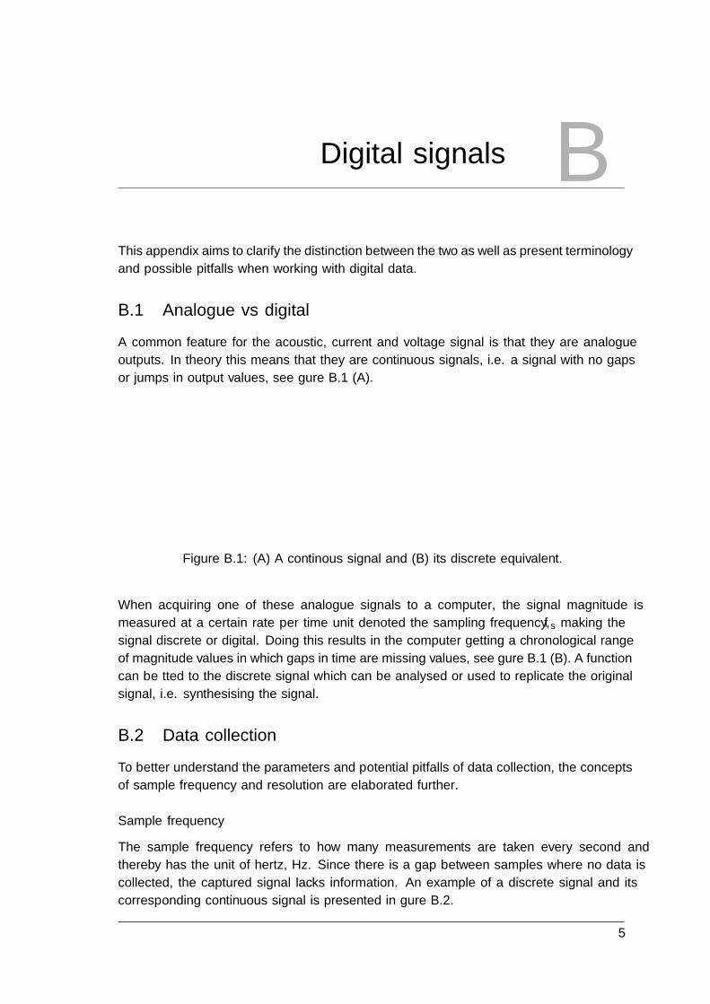
Digital signals BThis appendix aims to clarify the distinction between the two as well as present terminology
and possible pitfalls when working with digital data.
B.1 Analogue vs digital
A common feature for the acoustic, current and voltage signal is that they are analogue
outputs. In theory this means that they are continuous signals, i.e. a signal with no gaps
or jumps in output values, see �gure B.1 (A).
0 0.5 1 1.5 2
Time [s]
-1
-0.5
0
0.5
1
Am
plitu
de
(A) Continuos signal
0 0.5 1 1.5 2
Time [s]
-1
-0.5
0
0.5
1
Am
plitu
de(B) Discrete signal
Figure B.1: (A) A continous signal and (B) its discrete equivalent.
When acquiring one of these analogue signals to a computer, the signal magnitude is
measured at a certain rate per time unit denoted the sampling frequency, fs making the
signal discrete or digital. Doing this results in the computer getting a chronological range
of magnitude values in which gaps in time are missing values, see �gure B.1 (B). A function
can be �tted to the discrete signal which can be analysed or used to replicate the original
signal, i.e. synthesising the signal.
B.2 Data collection
To better understand the parameters and potential pitfalls of data collection, the concepts
of sample frequency and resolution are elaborated further.
Sample frequency
The sample frequency refers to how many measurements are taken every second and
thereby has the unit of hertz, Hz. Since there is a gap between samples where no data is
collected, the captured signal lacks information. An example of a discrete signal and its
corresponding continuous signal is presented in �gure B.2.
5
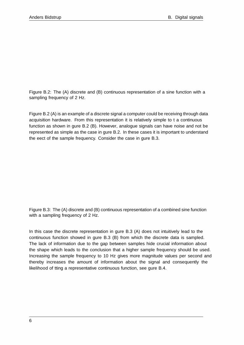
Anders Bidstrup B. Digital signals
0 2 4 6 8
Time
-2
-1
0
1
2
Am
plitu
de
(A) Discrete representation
0 2 4 6 8
Time
-2
-1
0
1
2
Am
plitu
de
(B) Continuous representation
Figure B.2: The (A) discrete and (B) continuous representation of a sine function with asampling frequency of 2 Hz.
Figure B.2 (A) is an example of a discrete signal a computer could be receiving through data
acquisition hardware. From this representation it is relatively simple to �t a continuous
function as shown in �gure B.2 (B). However, analogue signals can have noise and not be
represented as simple as the case in �gure B.2. In these cases it is important to understand
the e�ect of the sample frequency. Consider the case in �gure B.3.
0 2 4 6 8
Time
-2
-1
0
1
2
Am
plitu
de
(A) Discrete representation
0 2 4 6 8
Time
-2
-1
0
1
2
Am
plitu
de
(B) Continuous representation
Figure B.3: The (A) discrete and (B) continuous representation of a combined sine functionwith a sampling frequency of 2 Hz.
In this case the discrete representation in �gure B.3 (A) does not intuitively lead to the
continuous function showed in �gure B.3 (B) from which the discrete data is sampled.
The lack of information due to the gap between samples hide crucial information about
the shape which leads to the conclusion that a higher sample frequency should be used.
Increasing the sample frequency to 10 Hz gives more magnitude values per second and
thereby increases the amount of information about the signal and consequently the
likelihood of �tting a representative continuous function, see �gure B.4.
6
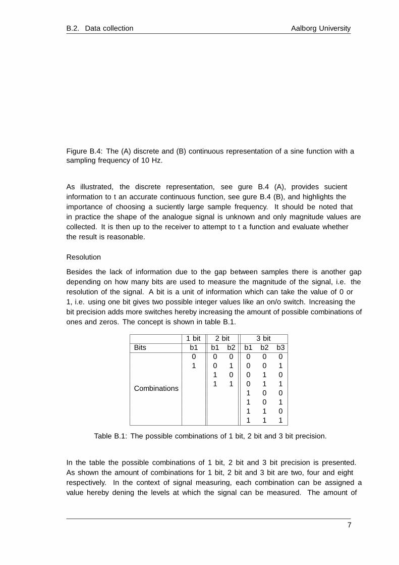
B.2. Data collection Aalborg University
0 2 4 6 8
Time
-2
-1
0
1
2
Am
plitu
de
(A) Discrete representation
0 2 4 6 8
Time
-2
-1
0
1
2
Am
plitu
de
(B) Continuous representation
Figure B.4: The (A) discrete and (B) continuous representation of a sine function with asampling frequency of 10 Hz.
As illustrated, the discrete representation, see �gure B.4 (A), provides su�cient
information to �t an accurate continuous function, see �gure B.4 (B), and highlights the
importance of choosing a su�ciently large sample frequency. It should be noted that
in practice the shape of the analogue signal is unknown and only magnitude values are
collected. It is then up to the receiver to attempt to �t a function and evaluate whether
the result is reasonable.
Resolution
Besides the lack of information due to the gap between samples there is another gap
depending on how many bits are used to measure the magnitude of the signal, i.e. the
resolution of the signal. A bit is a unit of information which can take the value of 0 or
1, i.e. using one bit gives two possible integer values like an on/o� switch. Increasing the
bit precision adds more switches hereby increasing the amount of possible combinations of
ones and zeros. The concept is shown in table B.1.
1 bit 2 bit 3 bitBits b1 b1 b2 b1 b2 b3
Combinations
0 0 0 0 0 01 0 1 0 0 1
1 0 0 1 01 1 0 1 1
1 0 01 0 11 1 01 1 1
Table B.1: The possible combinations of 1 bit, 2 bit and 3 bit precision.
In the table the possible combinations of 1 bit, 2 bit and 3 bit precision is presented.
As shown the amount of combinations for 1 bit, 2 bit and 3 bit are two, four and eight
respectively. In the context of signal measuring, each combination can be assigned a
value hereby de�ning the levels at which the signal can be measured. The amount of
7

Anders Bidstrup B. Digital signals
combinations is calculated as 2nbits which means that even a slight increase of the bit
precision can be advantageous if more magnitude levels are necessary.
0 2 4 6
Time
-1.5
-1
-0.5
0
0.5
1
1.5
Am
plitu
de(A) 2 bit precision
0 2 4 6
Time
-1.5
-1
-0.5
0
0.5
1
1.5
Am
plitu
de
(B) 4 bit precision
0 2 4 6
Time
-1.5
-1
-0.5
0
0.5
1
1.5
Am
plitu
de
(C) 8 bit precision
Figure B.5: A sine wave and its corresponding representation using (A) 2 bit, (B) 4 bitand (C) 8 bit precision with a sample frequency of 10 Hz.
On �gure B.5 a sine wave is presented with (A) 2 bit, (B) 4 bit and (C) 8 bit precision.
Note that even though the data is sampled at a rate of 10 Hz the resolution makes the
signal look like its sampled at a di�erent frequency. The choppiness of �gure B.5 (A)
makes the signal seem to be sampled at a signi�cantly lower frequency as a consequence of
the limited magnitude levels. This highlights the loss of data taking place which in some
cases could be critical. In the case of �gure B.5 (B) the increased amount of magnitude
levels result in a lowered amount of data loss and thereby a better data set for �tting a
continuous function. Further improvement is shown on �gure B.5 (C) where the discrete
and continuous sample can not be told apart.
When choosing the resolution for data acquisition it is necessary to consider the range of
possible measured values. In the case of having a 3 bit precision in the range of values
from -1 to 1 three situations are shown in �gure B.6.
0 2 4 6
Time
-1.5
-1
-0.5
0
0.5
1
1.5
Am
plitu
de
(A) Too high
0 2 4 6
Time
-1.5
-1
-0.5
0
0.5
1
1.5
Am
plitu
de
(B) Too low
0 2 4 6
Time
-1.5
-1
-0.5
0
0.5
1
1.5
Am
plitu
de
(C) Just right
Figure B.6: Acquiring a sine wave with an amplitude of (A) 1.5, (B) 0.5 and (C) 1.0 with3 bit precision on a range from -1 to 1.
In the case of �gure B.6 (A) a sine wave with an amplitude of 1.5 is measured. As indicated
on the graph the amplitude of the sine wave is too high compared to the range resulting in
the measuring equipment capping at 1.0. Consequently a loss of data near the peaks occur
8

B.2. Data collection Aalborg University
making the situation undesirable. In contrast �gure B.6 (B) shows the measured signal
for a sine wave with an amplitude of 0.5. In this case the sine wave does not utilise the
full range of the setup. Although the equipment is far from capping, by not using the full
range of the equipment, a low resolution is achieved relative to the potential of the setup.
Therefore, to reach the highest resolution possible the signal should take advantage of the
whole range of the equipment whilst avoiding capping as seen on �gure B.6 (C).
9


Digital filtering CThis appendix presents the basics of the design and e�ect of digital �lters through an
introduction to the two primary groups of �lter - FIR and IIR - and the sub-groups of
�lters - low-pass, high-pass, band-pass and band-stop.
C.1 Finite and in�nite impulse response �lters
There are two overall types of �lters - �nite impulse response, henceforth FIR, and in�nite
impulse response, henceforth IIR [World, 2012]. The di�erence between the two lie in
whether the �lter requires past outputs or not. If the �lter does not require past outputs
but is solely dependent on present and past inputs, it is an FIR �lter. Given a signal, x
as a function of the sample number, n, the output after implementing a FIR �lter could
be as in equation (C.1).
y(n) =x(n) + x(n− 1)
2(C.1)
The �lter used in this equation is a two-term average �lter and, as shown, only depends
on values of the input x. In contrast the IIR �lters use recursion. This means that the
�lter uses past outputs to calculate the new output as in the case of equation (C.2).
y(n) = x(n) + y(n− 1) (C.2)
In this case the newest signal value is added to the previous output value to create the
newest output.
C.2 Types of �lters
When moving past the overall classi�cation of FIR and IIR �lters, there is a sub-
classi�cation based on the e�ect of the �lter. In the case of applying a �lter to a signal
it is often desired to cut out part of the frequencies. Consequently a range of frequency-
selective �lters have been developed to cope with common cases. It should be noted that
the possibilities are endless when it comes to the speci�c functionality of a �lter even if they
are classi�ed as the same type. However, the four main groups are shown on �gure C.1.
11

Anders Bidstrup C. Digital �ltering
Figure C.1: Gain vs angular frequency plot of a low-pass, high-pass, band-pass and band-stop �lter [Aasvik, 2016]
The �rst �lter on the �gure is a low-pass �lter. As indicated by the gain-frequency plot
the principle with the �lter is to de�ne a cut-o� frequency at which the gain becomes zero.
In this way post-�ltering the signal only contains frequencies below the cut-o� frequency.
The inverse version of this is a high-pass �lter as shown on �gure C.1. In this case the
frequencies below the cut-o� frequency are removed whereas the rest is preserved. The two
remaining �lters are simply combinations of low-pass and high-pass �lters. By having a
low-pass �lter remove frequencies above some value followed by a high-pass �lter removing
frequencies below some value, a band-pass �lter is created. Similarly a band-stop �lter can
be made where the high-pass and low-pass �lters are used on the signal in parallel and
then combined to provide the �nal output. These are examples of some characteristics
digital �lters can have and are in no way an exhaustive list of the possibilities within the
subject.
12

Algorithm overview DIn this appendix the grouping of machine learning algorithms is based on the classi�cation
proposed by Dr. Jason Brownlee [Brownlee, 2013]. In an attempt to provide a graspable
overview the algorithms are grouped both by style and similarity.
D.1 Algorithm styles
The style of an algorithm refers to the way it interacts with the data or environment. In
this section four style groups are presented:
� Supervised learning
� Unsupervised learning
� Semi-supervised learning
� Reinforcement learning
Supervised learning
In this group the algorithms are trained by a data set with labelled data. This means that
for each set of input data the output is speci�ed. The algorithm uses this data to make
a model where new input data is provided with a suitable output based on the relations
found in the training data.
Unsupervised learning
This group stands in direct contrast to supervised learning in the sense that the data for
these algorithms is unlabelled. Being unaware of the output the algorithms in this group
search for structure in the data with the aim of spotting redundancies or extracting rules.
Semi-supervise learning
As the name suggests this group hosts algorithms fed with a mixture of labelled and
unlabelled data. The algorithms of this group combine the functionalities of the supervised
and unsupervised learning groups by attempting to develop a predictive model while
organising the unlabelled data.
Reinforcement learning
Lastly the group of reinforcement learning works with a changing environment. An agent
is set to interact with the environment to achieve a goal and makes decisions based on a
reward/punishment feedback system.
13

Anders Bidstrup D. Algorithm overview
D.2 Algorithms by similarity
Knowing the basic styles of algorithms makes it easier to understand the similarity between
algorithms. The grouping by similarity given by GP:
� Regression
� Instance-based algorithms
� Regularisation algorithms
� Decision tree algorithms
� Bayesian algorithms
� Clustering algorithms
� Association rule learning algorithms
� Arti�cial neural network algorithms
� Deep learning algorithms
� Dimensionality reduction algorithms
� Ensemble algorithms
Despite being thorough the grouping does not consider all algorithm. However, for the sake
of basic understanding of the possibilities within algorithm choice, each of the proposed
groups are presented in this section.
Regression
Regression models attempt to describe the trend of a training set based on an error
measurement. The type of output can either be continuous or discrete. An example
of regression with a continuous output is the case of linear regression where the model
can predict a speci�c value for each input data point. In case of the discrete output an
example is logistic regression which associates data regions with groups or classes, e.g.
spam/not-spam classi�cation.
Instance-based algorithms
In this group algorithms build a model which, based on a database of example data, classify
new data through a similarity measure.
Regularisation algorithms
Regularisation algorithms work as an extension to another method where they are used to
secure a simple model. They do this by penalising complexity and favouring simplicity of
the model to which it is an extension to.
Decision tree algorithms
As the name suggests the algorithms within this group consist of decision trees. A decision
tree is a tool that structures a range of decisions in a �ow chart manner. Starting from
the root decision it forks via branches to either zero nodes, meaning the outcome of the
branch, or n new decision nodes. Each of these decision nodes fork to extra decision nodes
until only outcomes remain. Once constructed, the tree consists of a range of decision rules
which can be used to predict the output or determine an action based on the input.
Bayesian algorithms
The group of bayesian algorithms consist solely of algorithms which apply Bayes' Theorem.
14

D.2. Algorithms by similarity Aalborg University
Clustering algorithms
The algorithms in this group use unlabelled data and attempt to �nd structure so that it
can be organised in groups, i.e. clusters.
Association rule learning algorithms
The algorithms contained in this group derive rules to explain relationships between
features.
Arti�cial neural network algorithms
Arti�cial neural networks are algorithms made to mimic the way the human brain works.
It consists of neurons which, based on an activation function, either take the value of one
or zero. The con�guration of ones and zeros are then used to determine the output based
on a set of input data.
Deep learning algorithms
Deep learning algorithms are neural networks which, as a consequence of technological
advances, are bigger and more complex than traditional arti�cial neural networks.
Dimensionality reduction algorithms
The algorithms in this group are used to highlight features which contribute the least to a
potential discrimination case. In this way the feature space can be reduced hereby freeing
computational power and making the training as well as usage of the algorithm faster.
Ensemble algorithms
This group refers to algorithms which produce a model using multiple independently
trained models to predict the output.
15


ANN structure andfunctionality E
In this appendix an introduction to the structure and functionality of the chosen ANN is
presented. The introduction includes descriptions of the visual representation of the ANN,
the used activation functions, the cost function, forward propagation, backpropagation
and how to calculate the derivative of the cost function. The chapter is primarily based
on the work of Michael Nielsen [Nielsen, 2017] but inspiration was drawn from Andrew Ng
of Stanford University [Ng, 2017] and Peter Roelants [Roelants, 2017].
E.1 Visual representation
To understand the structure of an ANN an example is shown on �gure E.1.
Figure E.1: Example of an arti�cial neural network with four layers.
A neural network consists of a range of connected neurons, as indicated by the circles
on �gure E.1, in di�erent layers. Each neuron, besides those in Layer 1, can assume a
value of either one or zero, i.e. activated or not, represented by a and the combination
17
Anders Bidstrup E. ANN structure and functionality
of activated and deactivated neurons is used for the prediction. Layer 1 is known as the
input layer and each neuron in the input layer represents a feature x. Layer 4 is known as
the output layer and represents the possible classes to map the input to. The remaining
internal layers are known as Hidden layers. The amount of input and output neurons
are determined by the amount of features considered and the amount of output classes
respectively. In contrast the amount of neurons in each hidden layer and the amount of
hidden layers are not �xed and no de�nitive rules exist to determine how many of each
should be present. Furthermore there is no rule specifying that the hidden layers have to
have the same amount of neurons, which increases the number of combinations further.
Lastly, as indicated by �gure E.1 the subscripted number on the a's is the neuron number,
i, from the top and the superscripted, parenthesised number on the a's is the layer in which
the neuron is, l. Similar notation is used for the parameters, or weights, denoted by Θ(l)ik .
Not included on �gure E.1 is what is known as the bias units. A bias unit is the neuron
of a given layer when i = 0 and has a constant value of one. Though not shown on the
�gure, they are included in the calculations.
E.2 Activation functions
To determine the activation of each neuron an activation function is required. The property
of such a function is to output either 0 or 1 when presented with an input. This can be
done by subjecting the result to a threshold as illustrated in the simple case of:
f(x) =
{1, if x > TH
0, if x < TH(E.1)
with f(x) being the activation function, x being the input and TH being a threshold.
Using only the threshold, the possibilities for the function f(x) are endless and the output
is discrete. However, for the use in ANN's, other properties are desired. Initially non-
linear functions are desired since introducing a non-linearity into the network allows the
approximation of non-linear function with networks containing just one hidden layer.
Furthermore the function should be continuously di�erentiable when using gradient-based
optimisation methods since the gradient of the activation is required in the calculation,
see section E.4.
In the case of this report, two activation functions are used. The �rst activation function
is the Sigmoid function and is used on all neurons in the hidden layers of the network. The
second activation function is the Softmax function which is only used in the output layer.
E.2.1 The Sigmoid function
The Sigmoid function is de�ned as:
g(xi) =1
1 + e−xi
and its shape is seen on �gure E.2.
18
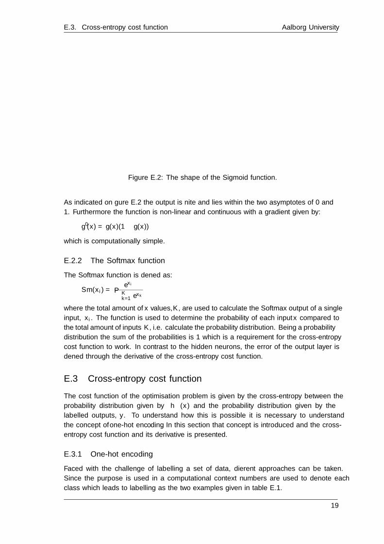
E.3. Cross-entropy cost function Aalborg University
-10 -8 -6 -4 -2 0 2 4 6 8 10
z
0
0.1
0.2
0.3
0.4
0.5
0.6
0.7
0.8
0.9
1
g(z)
The sigmoid function
Figure E.2: The shape of the Sigmoid function.
As indicated on �gure E.2 the output is �nite and lies within the two asymptotes of 0 and
1. Furthermore the function is non-linear and continuous with a gradient given by:
g′(x) = g(x)(1− g(x))
which is computationally simple.
E.2.2 The Softmax function
The Softmax function is de�ned as:
Sm(xi) =exi∑Kk=1 e
xk
where the total amount of x values, K, are used to calculate the Softmax output of a single
input, xi. The function is used to determine the probability of each input x compared to
the total amount of inputs K, i.e. calculate the probability distribution. Being a probability
distribution the sum of the probabilities is 1 which is a requirement for the cross-entropy
cost function to work. In contrast to the hidden neurons, the error of the output layer is
de�ned through the derivative of the cross-entropy cost function.
E.3 Cross-entropy cost function
The cost function of the optimisation problem is given by the cross-entropy between the
probability distribution given by hΘ(x) and the probability distribution given by the
labelled outputs, y. To understand how this is possible it is necessary to understand
the concept of one-hot encoding. In this section that concept is introduced and the cross-
entropy cost function and its derivative is presented.
E.3.1 One-hot encoding
Faced with the challenge of labelling a set of data, di�erent approaches can be taken.
Since the purpose is used in a computational context numbers are used to denote each
class which leads to labelling as the two examples given in table E.1.
19

Anders Bidstrup E. ANN structure and functionality
Class Sequential BinaryPedestrian 1 000Bicycle 2 001Scooter 3 010Car 4 011Bus 5 100Truck 6 101Train 7 110Other 8 111
Table E.1: Arbitrary classi�cation case with sequential and binary encoding.
Initially, the arbitrary classi�cation case is labelled using sequential numeric encoding.
Although each class has a unique digit an unintentional numerical hierarchy is established
which may a�ect the result of the computations at hand. The same problem is experienced
in the binary encoding shown in �gure E.1 in the amount of 1's the label contains.
To eliminate this problem a so-called one-hot encoding is used. The procedure starts by
creating a vector for each data point with the same amount of entries as there are classes.
Then the entry representing the correct class is set to 1 while the rest is set to zero. Doing
this for the case in table E.1 results in the labelling seen in table E.2.
Class One-hot encodingPedestrian [ 1 0 0 0 0 0 0 0 ]Bicycle [ 0 1 0 0 0 0 0 0 ]Scooter [ 0 0 1 0 0 0 0 0 ]Car [ 0 0 0 1 0 0 0 0 ]Bus [ 0 0 0 0 1 0 0 0 ]Truck [ 0 0 0 0 0 1 0 0 ]Train [ 0 0 0 0 0 0 1 0 ]Other [ 0 0 0 0 0 0 0 1 ]
Table E.2: Arbitrary classi�cation case with one-hot encoding.
As indicated in table E.2 the hierarchical trend is eliminated. Another aspect of this
encoding is that since the sum of the entries of a label vector is always 1, the vector can
be considered as a probability distribution where the probability of being the correct class
is 100 %. Gathering the label vectors for an entire data set results in a labelled output
matrix, y, to be used in the de�nition of the cost function.
E.3.2 The cost function and its derivative
Seeing as the hypothesis outputs a vector containing the probability distribution of
predicted classes of the network and the labelled output vector is a vector containing
the probability distribution for the actual output being a speci�c class, cross-entropy can
be used. Speci�cally cross-entropy is based on minimising the negative log-likelihood of a
set of weights being able to predict a class I. Using probability theory the likelihood of
a given set of weights resulting in a prediction of the correct class of each input can be
20
E.4. Training an ANN Aalborg University
simpli�ed as follows:
L(Θ|a(L),y) = P (y|a(L)) =I∏i=1
(a(L)i )yi
Using this expression the negative log-likelihood is given as:
−log(L(Θ|a(L),y)) = −log
(I∏i=1
(a(L)i )yi
)= −
I∑i=1
yi log(a(L)i )
Summing over the total amount of data point, M, gives the cost function, J(Θ):
J(Θ) = −M∑m=1
I∑i=1
ymi log(a(L)mi )
The equation for calculating the partial derivatives of the last layer in regards to the
weights is derived from the cost function. The result is:
δ
δΘ(L)ik
J(Θ) = a(L−1)k (a
(L)i − yi)
resulting in the overall optimisation problem of:
minΘ
J(Θ) = minΘ
(−
M∑m=1
I∑i=1
ymi log(a(L)mi )
)
E.4 Training an ANN
In order to train the hypothesis the minimisation problem presented in section E.3.2 is
performed using gradient descent. To understand the process of calculating the gradient
of the cost function, see section E.3.2, two new terms are introduced - Forward propagation
and Backpropagation.
Forward propagation
In the training process the ANN is subjected to a set of training data. Once a data point
(x(m), y(m)) is introduced, the process of forward propagation begins. This is the process
of calculating the activation of the neurons in the network starting from the input neurons.
In order to do so random initialisation of the weights is performed after which the process
can begin. Continuing the case from �gure E.1 the vectorised sequential process for one
data point is:
[1] a(1) = x(m)
[2] z(2) = Θ(2)a(1)
[3] a(2) = g(z(2))
[4] z(3) = Θ(3)a(2)
[5] a(3) = g(z(3))
[6] z(4) = Θ(4)a(3)
[7] a(4) = Sm(z(4)) = hΘ(x)
It should be noted that the bias term is included in the calculation of the activations with
the exclusion of the calculation for a(1).
21
Anders Bidstrup E. ANN structure and functionality
Backpropagation
Once forward propagation is �nished, backpropagation is performed to calculate error
terms for the neurons, δ(l)j . These are calculated to so that the remaining partial derivatives
of the cost function can be computed. The process of calculating the error terms is called
backpropagation since it starts from the output layer and goes backwards until the input
layer is reached. The sequential process is as follows:
[1] δ(4) = a(4) − y(m)
[2] δ(3) = (Θ(4))Tδ(4) � g′(z(3))
[3] δ(2) = (Θ(3))Tδ(3) � g′(z(2))
with � being the element-wise multiplication and g′(z) being the derivative of the sigmoid
function evaluated at z as presented in section E.2. Note that no error term is calculated for
the input layer. From these δ-vectors it is possible to calculate the remaining derivatives
of the cost function as:
δ
δΘ(l)ik
J(Θ) =
{δ
(l)i , if l 6= L and k = 0
a(l−1)k δ
(l)i , if l 6= L and k 6= 0
(E.2)
Computing the overall partial derivatives
With the formulae for calculating the partial derivatives of the cost function both for
the hidden layers, see section E.4, and the output layer, see section E.3.2, it is possible
to perform a non-regularised optimisation of the weights using a data set of one sample.
Introducing more data points leads to the introduction of an accumulator used to calculate
the partial derivatives of the cost function. This accumulator is denoted ∆ and is updated
after each back propagation by the following formula:
∆(l)ik =
∆
(l)ik + δ
(l)i , if l 6= L and k = 0
∆(l)ik + a
(l−1)k δ
(l)i , if l 6= L and k 6= 0
∆(l)ik + (a
(l)i − yi), if l = L and k = 0
∆(l)ik + a
(l−1)k (a
(l)i − yi), if l = L and k 6= 0
(E.3)
Once each data point in the training set is run through the forward propagation and
backpropagation the overall derivative of the cost function, D, can be calculated as:
D(l)ik =
1m∆
(l)ik , if k = 0
1m
(∆
(l)ik + λΘ
(l)ik
), if k 6= 0
(E.4)
As shown in the equations regularisation is not performed when k = 0 but is introduced
when k is one or above. Implementing these equations makes it possible to calculate the
gradient of the cost function. Hereby it is possible to perform gradient descent or more
advanced optimisation algorithms to minimise the cost in regards to the weights in Θ.
22

LabView program FIn this appendix the developed LabView program is presented. It consists of a main virtual
instrument, henceforth VI, and four sub-VI's. The main VI is shown in �gure F.1.
23

Anders Bidstrup F. LabView program
Figure F.1: The primary VI for data acquisition of sound, voltage and current.
24
Aalborg University
The VI should be read from left to right. Three structures are present in the VI:
� Sound acquisition while structure
� Sensor acquisition while structure
� Data saving case structure
The sound acquisition while structure reads data from the sound card and writes it to a
wave �le until the stop-button is activated. In order to specify how and from what the
loop should get the sound data a con�guration box is implemented before the loop. This
box requires inputs to specify how many data points to read at a time, whether continues
or �nite sampling is required, the device ID, the sample rate, the amount of channels to
capture sound from and the resolution of the signal. In this case it reads 11025 samples at
a time, reads data continuously, reads from the EDIROL UA-25 sound card, has a sample
rate of 44.1 kHz and captures sound on one channel with a resolution of 24 bit. Once
speci�ed it transfers the con�guration data into the while loop. Similarly an initiation box
for the wave �le is required. It speci�es the path and name of the �le to save the data in
and the type of data it will write to the �le. Once speci�ed the box opens the �le if it
exists or creates a new �le if it does not. The task is then transferred to the while loop.
Once the stop-button is pushed the while loop ends which triggers the program to close
the sound �le and clear the sound acquisition task.
The sensor acquisition while structure uses the DAQ Assistant. This is a sub-VI to read
data from a DAQ card and enables the user to specify which terminals to read from and at
what rate. In this case the data is sampled at 4 kHz and one data point is read at a time.
When the data is read it is outputted as a single signal. Since the signals need di�erent
conversions, it is demerged into the four measured signals being Sensor voltage, Sensor
current, Migatronic voltage and Migatronic current from top to bottom. The signals are
transferred into four separate sub-VI's to convert the signals to the actual current and
voltage after which the data points are pushed into a queue. Before this acquisition can
take place, the four queues need to be initialised. As for the con�guration and opening of
a sound �le for the sound acquisition, the queues are initialised outside the loop. For each
queue initialisation box two inputs are needed - the name of the queue and a constant to
symbolise the type of data to be stored in the queue. In this case the queues are named
Sensor_voltage, Sensor_current, Migatronic_voltage andMigatronic_current from top to
bottom and are fed a double type constant. The while loop reads and stores data in the
queues continuously until the stop button is pressed.
The last structure is the data saving case structure. A case structure has two states - True
and False - and a shift triggers the system inside the structure. In this case the structure is
made to empty the queues and write them to a spreadsheet �le with the event being that
the stop button is pressed. Since no data saving takes place before the stop buttons are
activated, the False state is an empty structure and therefore not included on �gure F.1.
The True state however, has four boxes to empty the queues and four boxes to release the
queues once emptied. The released data is then converted to dynamic signals and fed to a
Write to Measurement File VI. In this VI the signals are saved to a spreadsheet �le with
one time column and four data columns corresponding to the four signals acquired.
The VI's to convert each signal to the actual current and voltage are shown on �gure F.2.
25
Anders Bidstrup F. LabView program
Figure F.2: The conversion VI's for the four acquired signals.
The four VI's refer to the voltage probe signal, the current sensor signal, Migatronic
voltage measurement and Migatronic current measurement. The Migatronic conversions
are speci�ed in the datasheet, see enclosure A, as 0 - 10 V to 0 - 100 V and 0 - 10 V to 0 - 500
A for the voltage and current measurement respectively. Since the conversions are linear
the sub-VI's involve multiplying the acquired signal by a factor of 10 and 50, see �gure F.2.
The conversions for the implemented sensors are derived in section 9.4. The signal from
the voltage probe requires a correction of an o�set of 0.03 V followed by multiplication by
a factor of 0.52 to have the same value as the Migatronic voltage measurement. After this
a factor of 10 is used to convert the signal to the actual voltage based on the reference
value from the Migatronic measurement. In the case of the current sensor it is possible
to adjust the gain and o�set of the signal. To compensate for the settings of the sensor
initially the o�set, found to be 0.187 V, is subtracted from the signal. To convert the
signal to values similar to the Migatronic reference current measurement a factor of 1.53
is found. Since the signal is of the same magnitude as the reference value an additional
multiplication by a factor of 50 is implemented to convert the signal to the actual current.
26
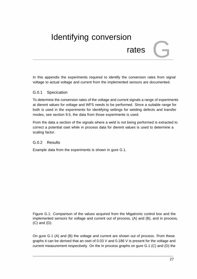
Identifying conversionrates G
In this appendix the experiments required to identify the conversion rates from signal
voltage to actual voltage and current from the implemented sensors are documented.
G.0.1 Speci�cation
To determine the conversion rates of the voltage and current signals a range of experiments
at di�erent values for voltage and WFS needs to be performed. Since a suitable range for
both is used in the experiments for identifying settings for welding defects and transfer
modes, see section 9.5, the data from those experiments is used.
From the data a section of the signals where a weld is not being performed is extracted to
correct a potential o�set while in process data for di�erent values is used to determine a
scaling factor.
G.0.2 Results
Example data from the experiments is shown in �gure G.1.
1.05 1.055 1.06 1.065 1.07
Sample ×104
0
2
4
Sig
nal s
tren
gth
[V]
(C) Voltage
1.05 1.055 1.06 1.065 1.07
Sample ×104
0
2
4
Sig
nal s
tren
gth
[V]
(D) Current
500 550 600 650 700
Sample
-0.02
0
0.02
0.04
Sig
nal s
tren
gth
[V]
(C) Voltage
SensorMigatronic
500 550 600 650 700
Sample
-0.1
0
0.1
0.2
0.3
Sig
nal s
tren
gth
[V]
(D) Current
Figure G.1: Comparison of the values acquired from the Migatronic control box and theimplemented sensors for voltage and current out of process, (A) and (B), and in process,(C) and (D).
On �gure G.1 (A) and (B) the voltage and current are shown out of process. From these
graphs it can be derived that an o�set of 0.03 V and 0.186 V is present for the voltage and
current measurement respectively. On the in process graphs on �gure G.1 (C) and (D) the
27

Anders Bidstrup G. Identifying conversion rates
o�set is already corrected. By inspection it is derived that scaling the voltage and current
signals by 0.52 and 1.53 respectively gives an acceptable result on the example data.
To check that the conversion is linear the conversions are tested on the data from the other
experiments. The values for both voltage and WFS are chosen in increments of two while
the travel speed is held constant at 1 mms . The converted signals from the experiments are
shown on �gure G.2.
1 1.02 1.04 1.06
Sample ×104
0
5
Sig
nal s
tren
gth
[V] (A) [1 0 0]
1 1.02 1.04 1.06
Sample ×104
0
5
Sig
nal s
tren
gth
[V] (F) [1 0 0]
1 1.02 1.04 1.06
Sample ×104
0
5
Sig
nal s
tren
gth
[V] (B) [1 2 -2]
1 1.02 1.04 1.06
Sample ×104
0
5
Sig
nal s
tren
gth
[V] (G) [1 2 -2]
1 1.02 1.04 1.06
Sample ×104
0
5
Sig
nal s
tren
gth
[V] (C) [1 4 -4]
1 1.02 1.04 1.06
Sample ×104
0
5
Sig
nal s
tren
gth
[V] (H) [1 4 -4]
1 1.02 1.04 1.06
Sample ×104
0
5
Sig
nal s
tren
gth
[V] (D) [1 -2 2]
1 1.02 1.04 1.06
Sample ×104
0
5
Sig
nal s
tren
gth
[V] (I) [1 -2 2]
1 1.02 1.04 1.06
Sample ×104
0
5
Sig
nal s
tren
gth
[V] (E) [1 -4 4]
1 1.02 1.04 1.06
Sample ×104
0
5
Sig
nal s
tren
gth
[V] (J) [1 -4 4]
SensorMigatronic
Figure G.2: Comparison of the values acquired from the Migatronic control box and theimplemented sensors from various experiments. The titles are of composition: [ Travelspeed - Voltage adjustment - WFS adjustment ].
On graphs (A) through (E) on �gure G.2 the converted voltage signal and the signal from
the Migatronic control box is compared. Similarly the converted current signal is compared
to the signal from the Migatronic control box on �gure G.2 (F) through (J). It should be
noted that the converted signals seem to follow the measurements from the Migatronic
control box which suggests that the conversion is linear and of su�cient precision.
28

Aalborg University
G.0.3 Comments
It is assessed that the conversion rates are of acceptable precision since the aim of the
conversion is to approximate the level of voltage and current.
29


Enclosure A:
Robotcontroller Interface for Flex 4000


Enclosure B:
Matlab program for feature extraction and
ANN training
The complete commented program and sub-functions can be found in "Program.zip"