Noname manuscript No.(will be inserted by the editor)

Topology optimization for minimum weight withcompliance and simplified nominal stress constraintsfor fatigue resistance

Maxime Collet · Matteo Bruggi · Pierre Duysinx

Received: date / Accepted: date

Abstract This work investigates a simplified ap-

proach to cope with the optimization of prelimi-

nary design of structures under local fatigue con-

straints along with a global enforcement on the

overall compliance. The problem aims at the min-

imization of the weight of linear elastic structures

under given loads and boundary conditions. The

expected stiffness of the optimal structure is pro-

vided by the global constraint, whereas a set of

local stress–based constraints ask for a structure

to be fatigue resistant. A modified Goodman fa-

tigue strength comparison is implemented through

the same formalism to address pressure–dependent

failure in materials as in Drucker–Prager strength

criterion. As a simplification, the Sines approach

is used to define the equivalent mean and alternat-

ing stresses to address the fatigue resistance for an

infinite life time. Sines computation is based onthe equivalent mean and alternate stress depend-

ing on the invariants of the stress tensor and its

Maxime ColletDepartment of Aerospace and Mechanical Engineering

University of Liege, 4000 Liege, Belgium

Tel.: +32-4-3669273Fax: +32-4-3669159

E-mail: maxime.collet@ulg.ac.be

Matteo Bruggi

Department of Civil and Environmental EngineeringPolitecnico di Milano, I20133, Milano, Italy

Tel.: +39-02-23994232Fax: +39-02-23994220E-mail: matteo.bruggi@polimi.it

Pierre Duysinx

Department of Aerospace and Mechanical EngineeringUniversity of Liege, 4000 Liege, Belgium

Tel.: +32-4-3669194

Fax: +32-4-3669159E-mail: p.duysinx@ulg.ac.be

deviatoric part, respectively. The so–called singu-

larity phenomenon is overcome by the implemen-

tation of a suitable qp-relaxation of the equivalent

stress measures. Numerical examples are presented

to illustrate the features of the achieved optimal

layouts and of the proposed algorithm.

Keywords topology optimization · fatigue

constraints · stress constraints · singularity

problem · Goodman criterion

1 Introduction

Topology optimization is formulated as the prob-

lem that finds the optimal distribution of a given

amount of material within a design domain, see

Bendsøe and Sigmund (2003). Since the seminal

work by Bendsøe and Kikuchi (1988), most devel-

opments of topology optimization have been based

on the minimization of the elastic strain energy

of the structure related to the external work of

the loads. This problem is commonly named the

minimization of the structural compliance or, in

other words, the maximization of the overall stiff-

ness. Today, aeronautical and mechanical indus-

tries consider topology optimization as a powerful

tool for conceptual design in engineering. However

in real life applications, a conventional compliance–

based topology optimization can not fully satisfy

the industrial needs. To produce structural parts

that fulfil specific functioning requirements, fail-

ure of the structure must be prevented at each

point of the component. Therefore, as pointed out

in Duysinx et al (2008), a stress–based topology

optimization is needed to propose a design that

can satisfy given stress–based requirements. Fur-

thermore, many aeronautical and automotive ap-

plications require that the life of a structure is pre-

served at least during a given amount of loading

cycles. In this way, the structure must be designed

such that it can sustain fatigue failure.

Compliance–based topology optimization is well

mastered and there are many successful results, see

for instance Eschenauer and Olhoff (2001), Roz-

vany (2009) and Bendsøe and Sigmund (2003) for

a comprehensive review. Conversely, stress–based

topology optimization was neglected, for a long

time, mainly because of many related numerical

issues. Since the last decades, a renewed interest

has been directed towards this approach as we

can seen from some milestone works, see Duysinx

and Bendsøe (1998), Duysinx and Sigmund (1998),

Svanberg et Werme (2007), Peirera et al (2004),

Paris et al (2009) and Guilherme et Fontsesca (2007)

for example. The main encountered issues in stress–

based topology optimization are the singularity phe-

nomenon and the large scale optimization problem

due to the local behavior of the stresses.

The so–called singularity phenomenon was ex-

tensively studied by Sved and Ginos (1968) and

Kirsch (1990), among the others. This phenomenon

can lead to non convergence issues, meaning that,

when the density approaches its lower bound, the

stress value is different from zero and the min-

imization algorithm is steered towards local so-

lutions full of gray regions. The singularity phe-

nomenon can be overcome through an appropriate

relaxation of the constraints in the optimization

problem. The so–called ε–relaxation was first pro-

posed by Cheng and Guo (1997). This method re-

sorts to the solution of a series of perturbed sub–

optimization problems with a decreasing value of a

relaxing parameter ε. Later on, Bruggi (2008) pro-

posed an alternative technique, the so–called qp–

relaxation, which adopts a different penalization

for the interpolation of stiffness (p) and apparent

“local” stresses (q).

An additional numerical issue affecting a stress–

based topology optimization is the large size of the

optimization problem. It is well established that

stress–based topology optimization leads to large

scale problems when the control of the stress mea-

sure is operated at each point of the structure.

That is to say that there are at least as many

constraints as the design variables are. This ap-

proach, called the local stress approach, was origi-

nally proposed by Duysinx and Bendsøe (1998). It

has been shown that the crucial point was the com-

putational effort to solve the optimization prob-

lem. A global stress approach, using aggregation

of the local constraints techniques either based on

the p-norm, the p-mean or the Kresselmeier Stein-

hauser (KS) function were proposed by Duysinx

and Sigmund (1998) and Yang and Chen (1996) to

overcome the issue related to the previous local ap-

proach. It was shown the the global CPU time was

effectively reduced, but the robustness of a local

control was generally lost. It must be also noticed

that, due to the highly non linear behavior of such

a global constraint, the resolution of the problem

can become unstable and parameter–dependant.

Luo et al (2013) proposed an enhanced aggrega-

tion technique based on the KS function which ag-

gregates separately the active and the passive lo-

cal stress constraints along with a relevant active

set strategy. The exposed method showed inter-

esting results but still requires a good tuning of

the numerical parameters. Between the local and

the global approach, Holmberg et al (2013, 2014)

used clustered stress constraints. The method is

based on the aggregation of the local stress con-

straints into clusters allowing for a decent control

of the local peak value of the stresses. The clas-

sical global approach is recovered when only one

cluster is used. The main issue when using the pro-

posed clustering method lies in the way to generate

clusters approximating suitably the local stresses.

Furthermore, it has been shown that the solution

depends on the number of clusters. An alternative

to reduce the CPU time was proposed by Bruggi

and Duysinx (2012, 2013) which consider a global

compliance constraint along with local stress con-

straints and an enhanced active–set strategy. Re-

sults showed that the number of local stress con-straints is highly reduced when stress peaks are

dealt with and the global compliance enforcement

is active. This leads to smaller CPU time even if

the number of stress constraints remains higher

than in a global or clustered approach.

When dealing with stress–based topology op-

timization, the possibility to take into account fa-

tigue within the optimization procedure is a nat-

ural extension of the available developments. Fa-

tigue is one of the most critical mode of failure in

many engineering applications such as aeronauti-

cal and automotive systems.. Today, transports ap-

plications seek for lighter and optimal design with

respect to environmental care and conservation.

Despite these obvious industrial needs, as pointed

out in Holmberg et al (2014), there is not a wide

literature about fatigue failure in topology opti-

mization, although some interesting issues were

2

explored concerning shape optimization, see e.g.

Mrzygold and Zielinski (2006), Kaya et al (2010),

Grunwald and Schnack (1997). The work by Holm-

berg et al (2014) introduces probability–based fa-

tigue constraints, which are aggregated through

the adoption of stress clusters. The contribution

in Svard (2015) deals with fatigue introducing an

assumption on the failure probability of a volume

element. It is based on the idea that the weakest

link model of failure developed by Weibull (1939)

takes a p-norm like form that is suitable for stress–

based topology optimization. The work in Seung et

al (2015) proposes another approach by incorpo-

rating dynamic fatigue and static failure criterion

under constant and proportional mechanical loads.

Aggregation methods are used to tackle local fa-

tigue constraints, whereas a differentiable form of

the signed von Mises criterion is implemented to

detect compressive and tensile stress states within

the design when defining the mean component of

the stress. Sherif et al (2010) used the concept

of the equivalent static load (ESL) in topology

optimization as shown in Park and Kang (2003)

and Kim and Park (2010) to sustain fatigue. This

approach uses a given tolerated damage as end–

criterion and looks after a design that fulfils the

constraints on the damage by performing several

FEM calculations coupled to a topology optimiza-

tion code. The main advantage of the proposed

procedure is that it can solve large scale prob-

lems. However, a full dynamic analysis is required

to generate the ESL, as well as fatigue calculation

to compute the most critical damage linked to the

relevant ESL.

Within the above framework, the present work

provides a simplified method that can improve con-

ventional compliance–based layouts with respect

to fatigue, adopting the mechanical design approach

of machine elements based on S–N diagrams or fa-

tigue criteria. This can be done resorting to an ex-

tension of the formulation proposed in Bruggi and

Duysinx (2012) for stress–constrained topology op-

timization of stiff structures with non–symmetric

strength in tension and compression. Indeed, the

Sines method, that is used to define an equiva-

lent stress measure for both the mean and alter-

nating component, respectively, is based on the

first and second invariants of the stress tensor, i.e

hydrostatic and deviatoric. To steer fatigue resis-

tance, a modified Goodman fatigue criterion is im-

plemented through the same formalism originally

adopted in Bruggi and Duysinx (2012) to address

pressure–dependent failure through the smooth

Drucker - Prager criterion. In the proposed formu-

lation, the compliance constraint deals with the

serviceability of the structure, enforcing a limit on

the displacement of the loaded point, whereas se-

lected active local constraints steer the optimizer

towards the achievement of fatigue–resistant lay-

outs, as required by industrial applications. The

proposed procedure is particularly effective when

limited regions of the design govern the collapse of

the structure.

The paper is organized as follows. Section 2

presents the Goodman failure criterion based on

the Sines method, along with the related equiv-

alent stress measures to be used in conjunction

with the SIMP material. The computation of the

stresses and fatigue criteria in the finite elements

formalism used in this work, i.e. a displacement–

based approximation, is also illustrated. Section3.1

presents the formulation of the topology optimiza-

tion problem which aims at the minimization of

the structural weight with compliance and fatigue

constraints. Section 3.3 mentions some numerical

issues, such as the adopted selection strategy for

stress constraints, the mathematical relaxation to

overcome the singularity problem and the limita-

tions experienced by conventional formulations of

topology optimization when coping with the ap-

proximation of the stress field. The sensitivity com-

putation is performed through the adjoint method,

as it is dealt with in Section 3.2. Section 4 presents

numerical results achieved through the above pro-

cedure, providing comparisons with optimal lay-

outs achieved by stress–based topology optimiza-

tion based the von Mises stress and fatigue stress

constraints. Section 5 concludes the paper, formu-lating remarks and drawing limitations of the pro-

posed preliminary design approach.

2 The fatigue failure criterion

This section aims at presenting the approach fol-

lowed in this paper to handle fatigue within a topol-

ogy optimization problem. The adopted procedure

follows the stress–based approach that is used for

fatigue design in machine design, see e.g. Budynas

and Nisbett (2011) and Norton (2000). This means

that the presented framework is valid only in the

high–cycle regime, i.e. for a very large number of

cycles (typically ≥ 103 although there is no real

consensus about the threshold between Low Cycle

Fatigue and High Cycle Fatigue). In the following,

it is assumed that we are in the case of High Cy-

cle Fatigue (HCF). It is important to pinpoint the

3

fact that HFC modeling works well when the loads

are known and predictable, meaning not random.

Furthermore, this approach is consistent as long

as the material remains elastic and no crack ini-

tiation is found. Finally, in absence of corrosion,

at room temperature and for a constant loading,

the quiescence of the solicitation has no influence

on the life of the structure and one has therefore

to only consider the amplitude, see Norton (2000).

In those conditions, the design can be performed

through a equivalent static analysis as discussed in

Section 2.2.

2.1 Sines method and modified Goodman criterion

Following the adopted assumptions of the former

paragraph, it is a general knowledge in machine

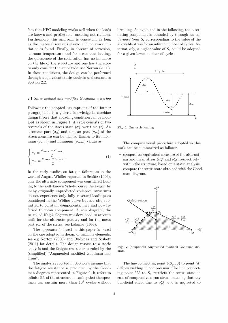
design theory that a loading condition can be mod-

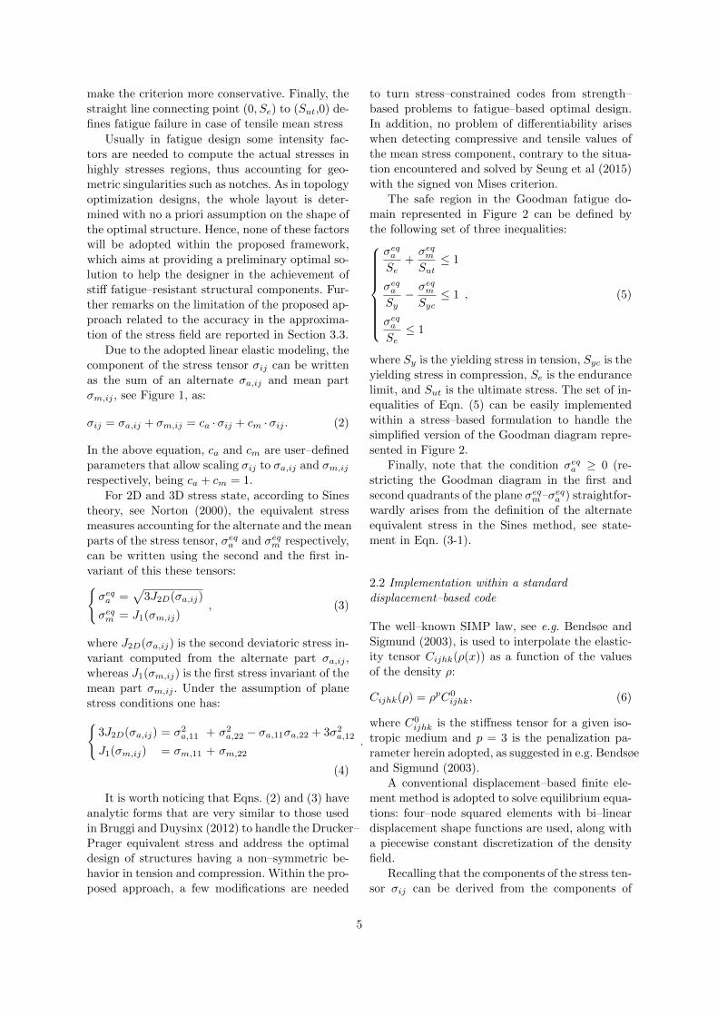
eled as shown in Figure 1. A cycle consists of two

reversals of the stress state (σ) over time (t). An

alternate part (σa) and a mean part (σm) of the

stress measure can be defined thanks to its maxi-

mum (σmax) and minimum (σmin) values as:σa =

σmax − σmin2

σm =σmax + σmin

2

. (1)

In the early studies on fatigue failure, as in the

work of August Wholer reported in Schutz (1996),

only the alternate component was considered lead-

ing to the well–known Wholer curve. As taught by

many originally unpredicted collapses, structures

do not experience only fully–reversed loadings as

considered in the Wolher curve but are also sub-

mitted to constant components, here and now re-

ferred to mean component. A new diagram, the

so–called Haigh diagram was developed to account

both for the alternate part σa and for the mean

part σm of the stress, see Lalanne (1999).

The approach followed in this paper is based

on the one adopted in design of machine elements,

see e.g Norton (2000) and Budynas and Nisbett

(2011) for details. The design resorts to a static

analysis and the fatigue resistance is ruled by the

(simplified) “Augmented modified Goodman dia-

gram”.

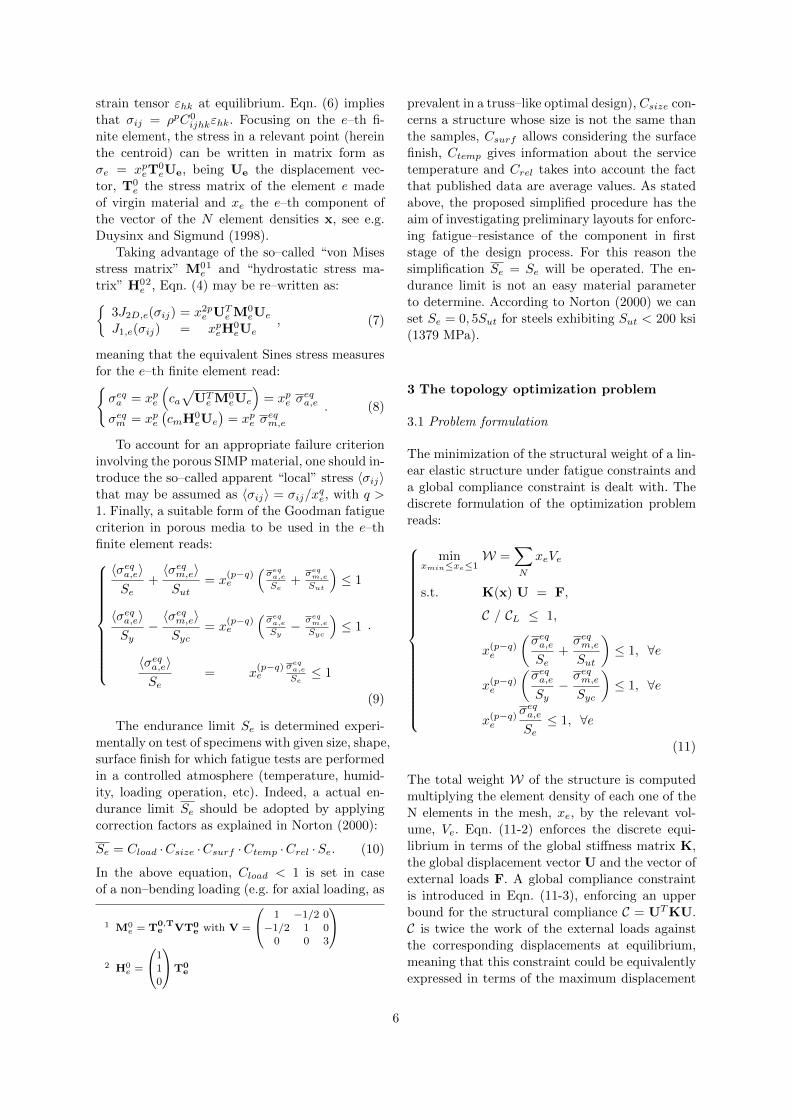
The analysis reported in Section 4 assume that

the fatigue resistance is predicted by the Good-

man diagram represented in Figure 2. It refers to

infinite life of the structure, meaning that the spec-

imen can sustain more than 107 cycles without

breaking. As explained in the following, the alter-

nating component is bounded by through an en-

durance limit Se corresponding to the value of the

allowable stress for an infinite number of cycles. Al-

ternatively, a higher value of Se could be adopted

for a given lower number of cycles.

t

σ

σm

σmin

σmax

σa

σa

1 cycle

Fig. 1 One cycle loading

The computational procedure adopted in this

work can be summarized as follows:

– compute an equivalent measure of the alternat-

ing and mean stress (σeqa and σeqm , respectively)

within the structure, based on a static analysis;

– compare the stress state obtained with the Good-

man diagram.

σeqm

σeqa

σeqaSe

σeqaSe− σeq

mSyc

σeqaSe

+σeqmSut

Safety region

Sut•

Se•

−Syc•

A•

Fig. 2 (Simplified) Augmented modified Goodman dia-gram

The line connecting point (-Syc, 0) to point ’A’

defines yielding in compression. The line connect-

ing point ’A’ to Se restricts the stress state in

case of compressive mean stress, meaning that any

beneficial effect due to σeqm < 0 is neglected to

4

make the criterion more conservative. Finally, the

straight line connecting point (0, Se) to (Sut,0) de-

fines fatigue failure in case of tensile mean stress

Usually in fatigue design some intensity fac-

tors are needed to compute the actual stresses in

highly stresses regions, thus accounting for geo-

metric singularities such as notches. As in topology

optimization designs, the whole layout is deter-

mined with no a priori assumption on the shape of

the optimal structure. Hence, none of these factors

will be adopted within the proposed framework,

which aims at providing a preliminary optimal so-

lution to help the designer in the achievement of

stiff fatigue–resistant structural components. Fur-

ther remarks on the limitation of the proposed ap-

proach related to the accuracy in the approxima-

tion of the stress field are reported in Section 3.3.

Due to the adopted linear elastic modeling, the

component of the stress tensor σij can be written

as the sum of an alternate σa,ij and mean part

σm,ij , see Figure 1, as:

σij = σa,ij + σm,ij = ca ·σij + cm ·σij . (2)

In the above equation, ca and cm are user–defined

parameters that allow scaling σij to σa,ij and σm,ijrespectively, being ca + cm = 1.

For 2D and 3D stress state, according to Sines

theory, see Norton (2000), the equivalent stress

measures accounting for the alternate and the mean

parts of the stress tensor, σeqa and σeqm respectively,

can be written using the second and the first in-

variant of this these tensors:{σeqa =

√3J2D(σa,ij)

σeqm = J1(σm,ij), (3)

where J2D(σa,ij) is the second deviatoric stress in-

variant computed from the alternate part σa,ij ,

whereas J1(σm,ij) is the first stress invariant of the

mean part σm,ij . Under the assumption of plane

stress conditions one has:{3J2D(σa,ij) = σ2

a,11 + σ2a,22 − σa,11σa,22 + 3σ2

a,12

J1(σm,ij) = σm,11 + σm,22.

(4)

It is worth noticing that Eqns. (2) and (3) have

analytic forms that are very similar to those used

in Bruggi and Duysinx (2012) to handle the Drucker–

Prager equivalent stress and address the optimal

design of structures having a non–symmetric be-

havior in tension and compression. Within the pro-

posed approach, a few modifications are needed

to turn stress–constrained codes from strength–

based problems to fatigue–based optimal design.

In addition, no problem of differentiability arises

when detecting compressive and tensile values of

the mean stress component, contrary to the situa-

tion encountered and solved by Seung et al (2015)

with the signed von Mises criterion.

The safe region in the Goodman fatigue do-

main represented in Figure 2 can be defined by

the following set of three inequalities:

σeqaSe

+σeqmSut≤ 1

σeqaSy− σeqmSyc≤ 1

σeqaSe≤ 1

, (5)

where Sy is the yielding stress in tension, Syc is the

yielding stress in compression, Se is the endurance

limit, and Sut is the ultimate stress. The set of in-

equalities of Eqn. (5) can be easily implemented

within a stress–based formulation to handle the

simplified version of the Goodman diagram repre-

sented in Figure 2.

Finally, note that the condition σeqa ≥ 0 (re-

stricting the Goodman diagram in the first and

second quadrants of the plane σeqm–σeqa ) straightfor-

wardly arises from the definition of the alternate

equivalent stress in the Sines method, see state-

ment in Eqn. (3-1).

2.2 Implementation within a standard

displacement–based code

The well–known SIMP law, see e.g. Bendsøe and

Sigmund (2003), is used to interpolate the elastic-

ity tensor Cijhk(ρ(x)) as a function of the values

of the density ρ:

Cijhk(ρ) = ρpC0ijhk, (6)

where C0ijhk is the stiffness tensor for a given iso-

tropic medium and p = 3 is the penalization pa-

rameter herein adopted, as suggested in e.g. Bendsøe

and Sigmund (2003).

A conventional displacement–based finite ele-

ment method is adopted to solve equilibrium equa-

tions: four–node squared elements with bi–linear

displacement shape functions are used, along with

a piecewise constant discretization of the density

field.

Recalling that the components of the stress ten-

sor σij can be derived from the components of

5

strain tensor εhk at equilibrium. Eqn. (6) implies

that σij = ρpC0ijhkεhk. Focusing on the e–th fi-

nite element, the stress in a relevant point (herein

the centroid) can be written in matrix form as

σe = xpeT0eUe, being Ue the displacement vec-

tor, T0e the stress matrix of the element e made

of virgin material and xe the e–th component of

the vector of the N element densities x, see e.g.

Duysinx and Sigmund (1998).

Taking advantage of the so–called “von Mises

stress matrix” M0e1 and “hydrostatic stress ma-

trix” H0e2, Eqn. (4) may be re–written as:{

3J2D,e(σij) = x2pe UTeM

0eUe

J1,e(σij) = xpeH0eUe

, (7)

meaning that the equivalent Sines stress measures

for the e–th finite element read:{σeqa = xpe

(ca√UTeM

0eUe

)= xpe σ

eqa,e

σeqm = xpe(cmH0

eUe

)= xpe σ

eqm,e

. (8)

To account for an appropriate failure criterion

involving the porous SIMP material, one should in-

troduce the so–called apparent “local” stress 〈σij〉that may be assumed as 〈σij〉 = σij/x

qe, with q >

1. Finally, a suitable form of the Goodman fatigue

criterion in porous media to be used in the e–th

finite element reads:

〈σeqa,e〉Se

+〈σeqm,e〉Sut

= x(p−q)e

(σeqa,e

Se+

σeqm,e

Sut

)≤ 1

〈σeqa,e〉Sy

−〈σeqm,e〉Syc

= x(p−q)e

(σeqa,e

Sy− σeq

m,e

Syc

)≤ 1

〈σeqa,e〉Se

= x(p−q)e

σeqa,e

Se≤ 1

.

(9)

The endurance limit Se is determined experi-

mentally on test of specimens with given size, shape,

surface finish for which fatigue tests are performed

in a controlled atmosphere (temperature, humid-

ity, loading operation, etc). Indeed, a actual en-

durance limit Se should be adopted by applying

correction factors as explained in Norton (2000):

Se = Cload ·Csize ·Csurf ·Ctemp ·Crel ·Se. (10)

In the above equation, Cload < 1 is set in case

of a non–bending loading (e.g. for axial loading, as

1 M0e = T0,T

e VT0e with V =

1 −1/2 0

−1/2 1 0

0 0 3

2 H0

e =

1

10

T0e

prevalent in a truss–like optimal design), Csize con-

cerns a structure whose size is not the same than

the samples, Csurf allows considering the surface

finish, Ctemp gives information about the service

temperature and Crel takes into account the fact

that published data are average values. As stated

above, the proposed simplified procedure has the

aim of investigating preliminary layouts for enforc-

ing fatigue–resistance of the component in first

stage of the design process. For this reason the

simplification Se = Se will be operated. The en-

durance limit is not an easy material parameter

to determine. According to Norton (2000) we can

set Se = 0, 5Sut for steels exhibiting Sut < 200 ksi

(1379 MPa).

3 The topology optimization problem

3.1 Problem formulation

The minimization of the structural weight of a lin-

ear elastic structure under fatigue constraints and

a global compliance constraint is dealt with. The

discrete formulation of the optimization problem

reads:

minxmin≤xe≤1

W =∑N

xeVe

s.t. K(x) U = F,

C / CL ≤ 1,

x(p−q)e

(σeqa,eSe

+σeqm,eSut

)≤ 1, ∀e

x(p−q)e

(σeqa,eSy−σeqm,eSyc

)≤ 1, ∀e

x(p−q)e

σeqa,eSe≤ 1, ∀e

(11)

The total weight W of the structure is computed

multiplying the element density of each one of the

N elements in the mesh, xe, by the relevant vol-

ume, Ve. Eqn. (11-2) enforces the discrete equi-

librium in terms of the global stiffness matrix K,

the global displacement vector U and the vector of

external loads F. A global compliance constraint

is introduced in Eqn. (11-3), enforcing an upper

bound for the structural compliance C = UTKU.

C is twice the work of the external loads against

the corresponding displacements at equilibrium,

meaning that this constraint could be equivalently

expressed in terms of the maximum displacement

6

allowed in the loaded region. In the following nu-

merical simulations, CL = αCC0, where C0 is the

compliance evaluated for the virgin material over

the full domain and αC is a prescribed parameter.

Eqns. (11-4,5,6) refer to the set of 3 ·N local stress

constraints on the equivalent Goodman/Sines stress

measures reported in Eqn. (9).

The problem in Eqn. (11) defines a minimum

weight formulation with compliance and fatigue

constraints, i.e. the MWCF problem. This formu-

lation may be exploited when safety against fatigue

failure is required along with a prescribed stiffness

at the serviceability limit state. This improves con-

ventional compliance–based layouts. Implementa-

tion of the MWCF formulation follows straight-

forwardly that of the minimum weight formula-

tion with compliance and stress constraints, i.e. the

MWCS problem investigated in Bruggi and Duys-

inx (2012).

It must be remarked that the adopted discretiza-

tion of the displacement and density field is af-

fected by the well–known checkerboard problem,

see e.g.Sigmund and Petersson (1998). Moreover,

a control of the thickness of the members resulting

from the optimization procedure is needed to avoid

mesh dependence. This work adopts the density–

based approach, see e.g. Bourdin (2001) and Bruns

and Tortorelli (2001). The consistent filter used in

this contribution follows the approach proposed in

the work byLe et al. (2010) where the original de-

sign variables xe are mapped into a new set of

physical unknown xe:

xe =1∑N Hei

∑N

Heixi,

Hei =∑N

max(0, rmin − dist(e, i)),(12)

where dist(e, i) is the distance between the cen-

troid of the e−th and i−th element, whereas rmin >

dm is the filter radius, and dm is the reference

length of the element edges. In the simulations pre-

sented next, rmin = 1, 5 dm is assumed.

3.2 Sensitivity analysis

This section deals with the sensitivity computation

for the local constraints in Eqn. (11-4,5,6)), as re-

quired at each iteration of the optimization proce-

dure. The derivative of the global compliance con-

straint C with respect to the density design vari-

ables is herein omitted since it is classic result for

the sake of brevity, see e.g. Bendsøe and Sigmund

(2003).

The derivatives of the equivalent “local” mea-

sures of the alternate and mean stress for the e–th

finite element, respectively σeqa,e and σeqm,e, with re-

spect to the density unknown xk can be formulated

as follows:

∂σeqa,e∂xk

= δek(p− q)xp−q−1e σeqa,e +∂σeqa,e∂xk

xp−qe

∂σeqm,e∂xk

= δek(p− q)xp−q−1e σeqm,e +∂σeqm,e∂xk

xp−qe .

(13)

The above equation requires the computation of

the sensitivity of σeqa,e and σeqm,e, which is caried

out through the adjoint method. Reminding Eqn.

(8), one has:

∂σeqa,e∂xk

= λT∂K

∂xkU, where

Kλ = −[ca(UTM0

eU)−12M0

eU]T,

(14)

and

∂σeqm,e∂xk

= µT∂K

∂xkU, where

Kµ = −[cmH0

e

]T.

(15)

In the above forms, λ and µ are the adjoint vectors

computed via the solution of each adjoint problem

of Eqns. (14) and (15). The solution of one addi-

tional (pseudo)–load case for the linear system in

Eqn. (11-2) is required per each (active) constraint.

As done in Bruggi and Duysinx (2012), the

stiffness matrix K is factorized at each iteration

before evaluating the constraints and their sensi-

tivities in order to speed up the computations.

3.3 Numerical issues and remarks

The optimization problem in Eqn. (11) is solved by

resorting mathematical programming approach,

adopting the Method of Moving Asymptotes by

Svanberg (1987).

When handling stress–based topology optimiza-

tion, a main issue is the so–called singularity phe-

nomenon, see e.g Cheng and Guo (1997) and Kirsch

(1990). Following Duysinx and Bendsøe (1998),

the same SIMP penalization p = q should ulti-

mately be assumed for both stiffness and “local”

stress interpolation. Due to the asymptotic behav-

ior of the apparent “local” stress in Eqn. (9), de-

generated sub–domains appear in the feasible do-

main and the optimizer based on KKT conditions

7

is likely to be stuck in a false optimum with mas-

sive grey regions, instead of the expected 0–1 de-

sign. A classical way to overcome this issue con-

sists in relaxing stress constraints. According to

the qp–approach proposed by Bruggi (2008), an

exponent q < p is adopted in the simulations to

provide a strong relaxation in the regions of low

density, without introducing any bias at full den-

sity. In the first iterations q = 2.6 is adopted to

highly relax the problem and encourage the acti-

vation of the global compliance constraint speed-

ing up the optimization solution. Afterwards the

value of the relaxing parameter q is gradually in-

creased to q = 2.75. Indeed, preliminary numerical

tests have shown that the adaptive version of this

relaxation leads to a more efficient solution.

A lower bound xmin > 0 is needed for each den-

sity design variable xe to avoid singularity of the

global stiffness matrix when solving Eqn. (11-2).

The assumption xmin = 10−3 has been adopted in

Section 4 to provide numerical results, as recom-

mended Bendsøe and Sigmund (2003). Numerical

tests have shown that the adopted implementa-

tion of the relaxed stress–constrained formulation

in Eqn. (11) is not sensitive with respect to a vari-

ation of xmin in the range 10−3–10−5.

Active restriction has been implemented to re-

duce the computational effort in terms of sensi-

tivity computation and MMA optimization. Sets

of active constraints with dimension Na are pro-

cessed during the optimization instead of the full

set of 3 ·N local constraints. Only the local stress

constraints whose value is larger than 0, 65 are con-

sidered as potentially active during the first itera-

tion. This threshold is progressively increased in 10

steps and constantly set to 0, 85 thereafter, see in

particular Bruggi and Duysinx (2013). The num-

ber of active constraints changes during the op-

timization, thus introducing discontinuities in the

multi–constrained minimization. Within the pro-

posed MWCF formulation, the global compliance

constraint has a crucial role in smoothing any dis-

continuity arising during the optimization because

of the adopted selection strategy, see further com-

ments in Section 4.2.

A final but crucial remark addresses the lack of

accuracy affecting the approximation of the stress

field in discretized problems of topology optimiza-

tion. The CPU cost drastically limits the refine-

ment of the finite elements mesh, meaning that,

quite often, the adopted finite elements approxi-

mation does not succeed in predicting with high

accuracy the exact value of a stress concentra-

tion, especially in case of local overstressings due

to geometrical details. Conventional schemes are

generally able to detect at least the location of a

stress concentration, thus leading to optimal lay-

outs whose shape carefully avoid stress concentra-

tion and exhibit the general stress flows. On this

point, reference is made in particular to the com-

prehensive review by Le et al. (2010) which ad-

dresses several numerical experiments reported in

the literature for the stress–based design of the L–

shaped cantilever.

As extensively pointed out in Svard (2015), nu-

merical inaccuracy in the evaluation of the stress

field is also due to the jagged nature of the optimal

structure arising in the fixed finite element mesh

used to handle the design domain. At the bound-

aries of the optimal layout, the transition from full

material 1 to void material xmin through the grey

region due to the filter, see Eqn. (12), may result

in an unexpected oscillation of the stresses over

the jagged boundary following the mesh, thus af-

fecting the stress–based optimal design. To solve

this problem, Svard (2015) proposes the adoption

of a combined approach that consists of an inte-

rior value extrapolation for the stresses across the

boundary. Effective results are shown adopting this

approach which is not implemented here but could

be conveniently implemented within the proposed

approach to improve the accuracy of the method

in future works.

4 Numerical simulations

The following examples focus on compliance–con-

strained fatigue–based topology optimization (MWCF

problems) versus compliance–constrained strength–

based topology optimization using the von Mises

criterion (MWCS problem), see in particular Bruggi

and Duysinx (2012). Geometry and boundary con-

ditions for the numerical applications are repre-

sented in Figure 3, where black zones are non–

design regions surrounding the applied point loads

to avoid the overstress due to singularities in the

application of the load. The number of finite ele-

ments for each discretization is shown in Table 1.

In case of fatigue–based problems, three com-

binations of the weighting factors in Eqn. (2), caand cm, are explored to investigate the sensitivity

of the designs with respect to the ratio between

the alternate component and respect to the mean

stress, see Table 1.

A reference material with Young modulus E =

1N/m2 and Poisson’s ratio ν = 0, 3 is considered

8

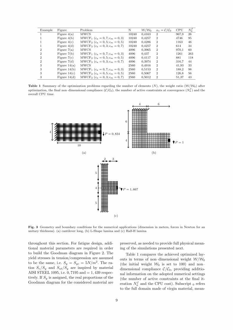
Example Figure Problem N W/W0 αc = C/C0 CPU Nfa

1 Figure 4(a) MWCS 10240 0,4163 2 967,9 261 Figure 4(b) MWCF1 (ca = 0, 7; cm = 0, 3) 10240 0,4257 2 4746 95

1 Figure 4(c) MWCF2 (ca = 0, 5; cm = 0, 5) 10240 0,4286 2 1163 461 Figure 4(d) MWCF3 (ca = 0, 3; cm = 0, 7) 10240 0,4257 2 614 34

2 Figure 7(a) MWCS 4096 0,3965 2 970,1 60

2 Figure 7(b) MWCF1 (ca = 0, 7; cm = 0, 3) 4096 0,437 2 1261 2632 Figure 7(c) MWCF2 (ca = 0, 5; cm = 0, 5) 4096 0,4117 2 881 118

2 Figure 7(d) MWCF3 (ca = 0, 3; cm = 0, 7) 4096 0,3974 2 316,7 44

3 Figure 14(a) MWCS 2560 0,4916 2 41,93 333 Figure 14(b) MWCF1 (ca = 0, 7; cm = 0, 3) 2560 0,5153 2 188,2 98

3 Figure 14(c) MWCF2 (ca = 0, 5; cm = 0, 5) 2560 0,5067 2 126,8 56

3 Figure 14(d) MWCF3 (ca = 0, 3; cm = 0, 7) 2560 0,5012 2 51,37 43

Table 1 Summary of the optimization problems regarding the number of elements (N), the weight ratio (W/W0) after

optimization, the final non–dimensional compliance (C/C0), the number of active constraints at convergence (Nfa ) and the

overall CPU time.

P = 0, 834

10

4

(a)

P = 14

6

4 6

(b)

P = 1, 667

5

4

5

2 3

(c)

Fig. 3 Geometry and boundary conditions for the numerical applications (dimension in meters, forces in Newton for an

unitary thickness). (a) cantilever long, (b) L-Shape lamina and (c) Half-H lamina

throughout this section. For fatigue design, addi-

tional material parameters are required in order

to build the Goodman diagram in Figure 2. The

yield stresses in tension/compression are assumed

to be the same, i.e. Sy = Syc = 5N/m2. The ra-

tios Se/Sy and Sut/Sy are inspired by material

AISI STEEL 1095, i.e. 0, 7195 and = 1, 439 respec-

tively. If Sy is assigned, the real proportions of the

Goodman diagram for the considered material are

preserved, as needed to provide full physical mean-

ing of the simulations presented next.

Table 1 compares the achieved optimized lay-

outs in terms of non–dimensional weight W/W0

(the initial weight W0 is set to 100) and non–

dimensional compliance C/C0, providing additio-

nal information on the adopted numerical settings

(the number of active constraints at the final it-

eration Nfa and the CPU cost). Subscript 0 refers

to the full domain made of virgin material, mean-

9

ing that weight and compliance at convergence are

normalized with respect to reference values at the

first iteration of the optimization procedure, when

xe = 1,∀e.Optimized layouts are presented in terms of

the physical unknowns xe of Eqn. (12) and are

endowed with maps representing the element–wise

equivalent stress measure σeqGD,max for fatigue–based

layouts, or σeqVM,max for strength–based results. For

each example all the maps are normalized to get

bounded within zero stress (blue regions) and the

maximum equivalent stress (red regions).

The maximum l.h.s. of the sets of constraints

in the Goodman criterion reads, see Eqn. (5):

σeqGD,max = max(σeqaSe

+σeqmSut

,σeqaSy− σeqmSyc

,σeqaSe

). (16)

In fact, the Goodman criterion is enforced through

three sets of inequalities and the value σeqGD,maxis the largest among the constraints prescribed by

the criterion. The maximum l.h.s. of a conventional

Von Mises constraint is given by:

σeqVM,max =σeqaSy

. (17)

4.1 Example 1. The long cantilever

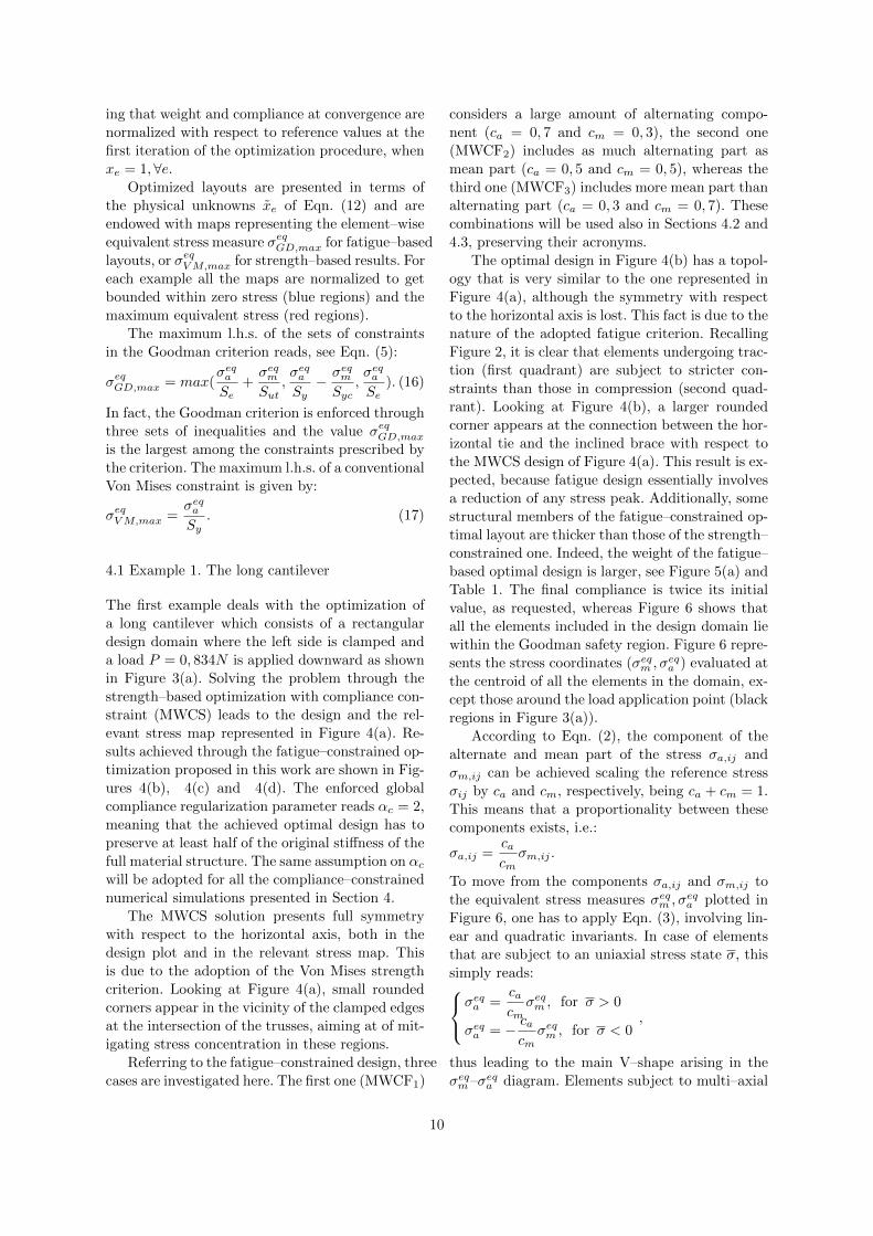
The first example deals with the optimization of

a long cantilever which consists of a rectangular

design domain where the left side is clamped and

a load P = 0, 834N is applied downward as shown

in Figure 3(a). Solving the problem through the

strength–based optimization with compliance con-

straint (MWCS) leads to the design and the rel-

evant stress map represented in Figure 4(a). Re-

sults achieved through the fatigue–constrained op-

timization proposed in this work are shown in Fig-

ures 4(b), 4(c) and 4(d). The enforced global

compliance regularization parameter reads αc = 2,

meaning that the achieved optimal design has to

preserve at least half of the original stiffness of the

full material structure. The same assumption on αcwill be adopted for all the compliance–constrained

numerical simulations presented in Section 4.

The MWCS solution presents full symmetry

with respect to the horizontal axis, both in the

design plot and in the relevant stress map. This

is due to the adoption of the Von Mises strength

criterion. Looking at Figure 4(a), small rounded

corners appear in the vicinity of the clamped edges

at the intersection of the trusses, aiming at of mit-

igating stress concentration in these regions.

Referring to the fatigue–constrained design, three

cases are investigated here. The first one (MWCF1)

considers a large amount of alternating compo-

nent (ca = 0, 7 and cm = 0, 3), the second one

(MWCF2) includes as much alternating part as

mean part (ca = 0, 5 and cm = 0, 5), whereas the

third one (MWCF3) includes more mean part than

alternating part (ca = 0, 3 and cm = 0, 7). These

combinations will be used also in Sections 4.2 and

4.3, preserving their acronyms.

The optimal design in Figure 4(b) has a topol-

ogy that is very similar to the one represented in

Figure 4(a), although the symmetry with respect

to the horizontal axis is lost. This fact is due to the

nature of the adopted fatigue criterion. Recalling

Figure 2, it is clear that elements undergoing trac-

tion (first quadrant) are subject to stricter con-

straints than those in compression (second quad-

rant). Looking at Figure 4(b), a larger rounded

corner appears at the connection between the hor-

izontal tie and the inclined brace with respect to

the MWCS design of Figure 4(a). This result is ex-

pected, because fatigue design essentially involves

a reduction of any stress peak. Additionally, some

structural members of the fatigue–constrained op-

timal layout are thicker than those of the strength–

constrained one. Indeed, the weight of the fatigue–

based optimal design is larger, see Figure 5(a) and

Table 1. The final compliance is twice its initial

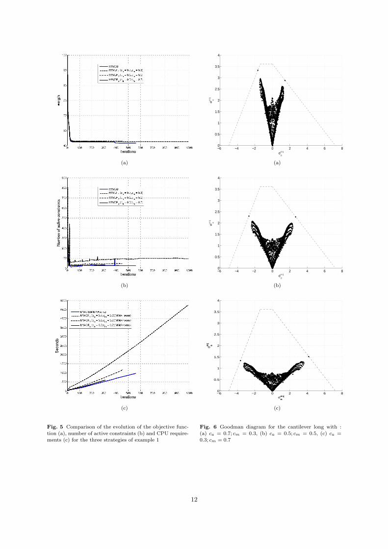
value, as requested, whereas Figure 6 shows that

all the elements included in the design domain lie

within the Goodman safety region. Figure 6 repre-

sents the stress coordinates (σeqm , σeqa ) evaluated at

the centroid of all the elements in the domain, ex-

cept those around the load application point (black

regions in Figure 3(a)).

According to Eqn. (2), the component of the

alternate and mean part of the stress σa,ij and

σm,ij can be achieved scaling the reference stress

σij by ca and cm, respectively, being ca + cm = 1.

This means that a proportionality between these

components exists, i.e.:

σa,ij =cacm

σm,ij .

To move from the components σa,ij and σm,ij to

the equivalent stress measures σeqm , σeqa plotted in

Figure 6, one has to apply Eqn. (3), involving lin-

ear and quadratic invariants. In case of elements

that are subject to an uniaxial stress state σ, this

simply reads:σeqa =cacm

σeqm , for σ > 0

σeqa = − cacm

σeqm , for σ < 0,

thus leading to the main V–shape arising in the

σeqm–σeqa diagram. Elements subject to multi–axial

10

stress states give rise to the remaining cloud of

points.

A very limited number of points are located

along the boundary of the fatigue criterion, corre-

sponding to the few fully stressed elements with

regard to the equivalent measure σeqGD,max in the

map of Figure 4(b). These elements are crucial

from a mechanical point of view, since their stress

regime governs the fatigue–constrained design. A

wider set of constraints control the numerical pro-

cedure since the active constraints selection strat-

egy is not limited to the fully–stressed elements,

see Section 3.3.

When a lower percentage of alternating compo-

nent is considered within the optimization prob-

lem, the optimal layouts and stress maps illus-

trated in Figure 4(c) and 4(d) are found. The

topology achieved for these examples is different

than in the previous simulations. Two members

are needed near the loading area instead of one,

as it was the case both for the MWCS and for

the MWCF1 problem. Assuming the weight of the

MWCS design as a reference, a heavier structure

arises for the topology in Figure 4(c), whereas nearly

the same weight is found for the layout represented

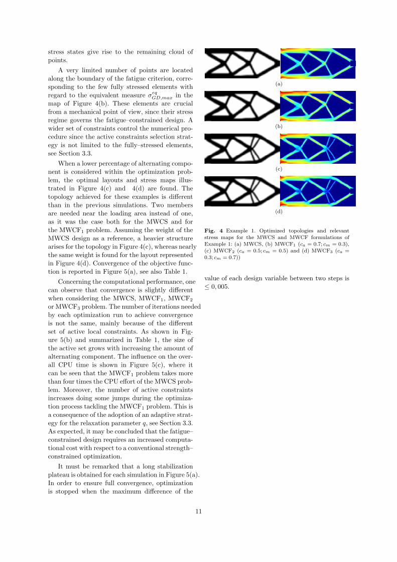
in Figure 4(d). Convergence of the objective func-

tion is reported in Figure 5(a), see also Table 1.

Concerning the computational performance, one

can observe that convergence is slightly different

when considering the MWCS, MWCF1, MWCF2

or MWCF3 problem. The number of iterations needed

by each optimization run to achieve convergence

is not the same, mainly because of the different

set of active local constraints. As shown in Fig-

ure 5(b) and summarized in Table 1, the size of

the active set grows with increasing the amount of

alternating component. The influence on the over-

all CPU time is shown in Figure 5(c), where it

can be seen that the MWCF1 problem takes more

than four times the CPU effort of the MWCS prob-

lem. Moreover, the number of active constraints

increases doing some jumps during the optimiza-

tion process tackling the MWCF1 problem. This is

a consequence of the adoption of an adaptive strat-

egy for the relaxation parameter q, see Section 3.3.

As expected, it may be concluded that the fatigue–

constrained design requires an increased computa-

tional cost with respect to a conventional strength–

constrained optimization.

It must be remarked that a long stabilization

plateau is obtained for each simulation in Figure 5(a).

In order to ensure full convergence, optimization

is stopped when the maximum difference of the

(a)

(b)

(c)

(d)

Fig. 4 Example 1. Optimized topologies and relevant

stress maps for the MWCS and MWCF formulations of

Example 1: (a) MWCS, (b) MWCF1 (ca = 0.7; cm = 0.3),(c) MWCF2 (ca = 0.5; cm = 0.5) and (d) MWCF3 (ca =

0.3; cm = 0.7))

value of each design variable between two steps is

≤ 0, 005.

11

(a)

(b)

(c)

Fig. 5 Comparison of the evolution of the objective func-tion (a), number of active constraints (b) and CPU require-

ments (c) for the three strategies of example 1

−6 −4 −2 0 2 4 6 80

0.5

1

1.5

2

2.5

3

3.5

4

σmeq

σaeq

(a)

−6 −4 −2 0 2 4 6 80

0.5

1

1.5

2

2.5

3

3.5

4

σmeq

σaeq

(b)

−6 −4 −2 0 2 4 6 80

0.5

1

1.5

2

2.5

3

3.5

4

σmeq

σ aeq

(c)

Fig. 6 Goodman diagram for the cantilever long with :

(a) ca = 0.7; cm = 0.3, (b) ca = 0.5; cm = 0.5, (c) ca =0.3; cm = 0.7

12

4.2 Example 2. The L–shaped plate

The second example deals with the well–known L–

shaped plate for which boundary conditions and

loads (P = 1N) are represented in Figure 3(b). As

in the previous section, the strength–constrained

problem is assumed as the reference case, whereas

problems of fatigue–based design are considered

for the three combinations of weighting factors caand cm introduced above.

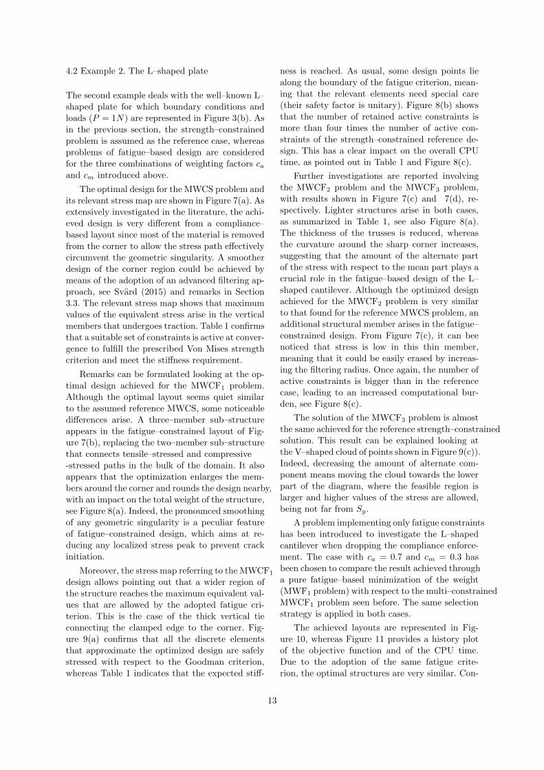
The optimal design for the MWCS problem and

its relevant stress map are shown in Figure 7(a). As

extensively investigated in the literature, the achi-

eved design is very different from a compliance–

based layout since most of the material is removed

from the corner to allow the stress path effectively

circumvent the geometric singularity. A smoother

design of the corner region could be achieved by

means of the adoption of an advanced filtering ap-

proach, see Svard (2015) and remarks in Section

3.3. The relevant stress map shows that maximum

values of the equivalent stress arise in the vertical

members that undergoes traction. Table 1 confirms

that a suitable set of constraints is active at conver-

gence to fulfill the prescribed Von Mises strength

criterion and meet the stiffness requirement.

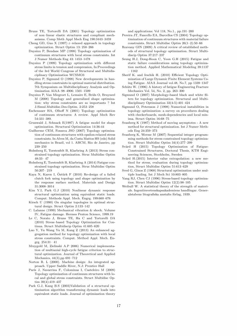
Remarks can be formulated looking at the op-

timal design achieved for the MWCF1 problem.

Although the optimal layout seems quiet similar

to the assumed reference MWCS, some noticeable

differences arise. A three–member sub–structure

appears in the fatigue–constrained layout of Fig-

ure 7(b), replacing the two–member sub–structure

that connects tensile–stressed and compressive

-stressed paths in the bulk of the domain. It also

appears that the optimization enlarges the mem-

bers around the corner and rounds the design nearby,

with an impact on the total weight of the structure,

see Figure 8(a). Indeed, the pronounced smoothing

of any geometric singularity is a peculiar feature

of fatigue–constrained design, which aims at re-

ducing any localized stress peak to prevent crack

initiation.

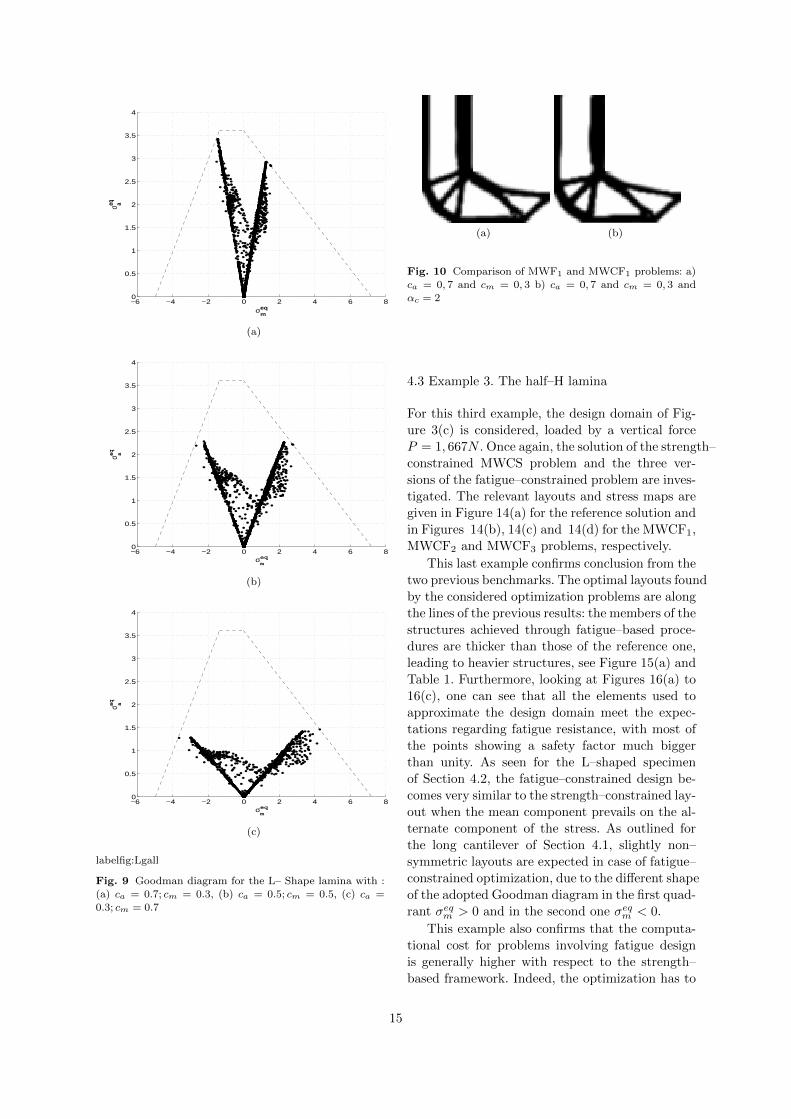
Moreover, the stress map referring to the MWCF1

design allows pointing out that a wider region of

the structure reaches the maximum equivalent val-

ues that are allowed by the adopted fatigue cri-

terion. This is the case of the thick vertical tie

connecting the clamped edge to the corner. Fig-

ure 9(a) confirms that all the discrete elements

that approximate the optimized design are safely

stressed with respect to the Goodman criterion,

whereas Table 1 indicates that the expected stiff-

ness is reached. As usual, some design points lie

along the boundary of the fatigue criterion, mean-

ing that the relevant elements need special care

(their safety factor is unitary). Figure 8(b) shows

that the number of retained active constraints is

more than four times the number of active con-

straints of the strength–constrained reference de-

sign. This has a clear impact on the overall CPU

time, as pointed out in Table 1 and Figure 8(c).

Further investigations are reported involving

the MWCF2 problem and the MWCF3 problem,

with results shown in Figure 7(c) and 7(d), re-

spectively. Lighter structures arise in both cases,

as summarized in Table 1, see also Figure 8(a).

The thickness of the trusses is reduced, whereas

the curvature around the sharp corner increases,

suggesting that the amount of the alternate part

of the stress with respect to the mean part plays a

crucial role in the fatigue–based design of the L–

shaped cantilever. Although the optimized design

achieved for the MWCF2 problem is very similar

to that found for the reference MWCS problem, an

additional structural member arises in the fatigue–

constrained design. From Figure 7(c), it can bee

noticed that stress is low in this thin member,

meaning that it could be easily erased by increas-

ing the filtering radius. Once again, the number of

active constraints is bigger than in the reference

case, leading to an increased computational bur-

den, see Figure 8(c).

The solution of the MWCF3 problem is almost

the same achieved for the reference strength–constrained

solution. This result can be explained looking at

the V–shaped cloud of points shown in Figure 9(c)).

Indeed, decreasing the amount of alternate com-

ponent means moving the cloud towards the lower

part of the diagram, where the feasible region is

larger and higher values of the stress are allowed,

being not far from Sy.

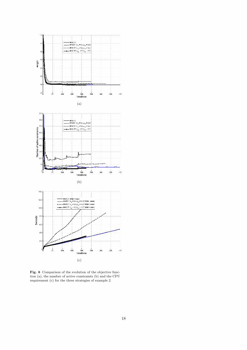
A problem implementing only fatigue constraints

has been introduced to investigate the L–shaped

cantilever when dropping the compliance enforce-

ment. The case with ca = 0.7 and cm = 0.3 has

been chosen to compare the result achieved through

a pure fatigue–based minimization of the weight

(MWF1 problem) with respect to the multi–constrained

MWCF1 problem seen before. The same selection

strategy is applied in both cases.

The achieved layouts are represented in Fig-

ure 10, whereas Figure 11 provides a history plot

of the objective function and of the CPU time.

Due to the adoption of the same fatigue crite-

rion, the optimal structures are very similar. Con-

13

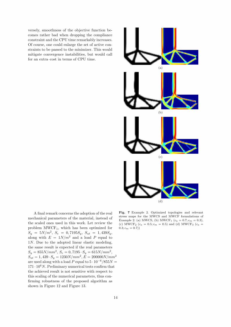
versely, smoothness of the objective function be-

comes rather bad when dropping the compliance

constraint and the CPU time remarkably increases.

Of course, one could enlarge the set of active con-

straints to be passed to the minimizer. This would

mitigate convergence instabilities, but would call

for an extra–cost in terms of CPU time.

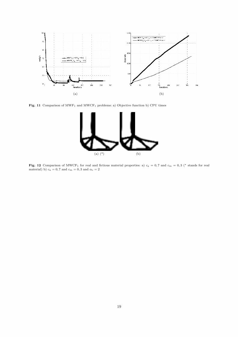
A final remark concerns the adoption of the real

mechanical parameters of the material, instead of

the scaled ones used in this work. Let review the

problem MWCF1, which has been optimized for

Sy = 5N/m2, Se = 0, 7195Sy, Sut = 1, 439Sy,

along with E = 1N/m2 and a load P equal to

1N . Due to the adopted linear elastic modeling,

the same result is expected if the real parameters

Sy = 855N/mm2, Se = 0, 7195 ·Sy = 615N/mm2,

Sut = 1, 439 ·Sy = 1230N/mm2, E = 200000N/mm2

are used along with a load P equal to 5 · 10−6/855N =

171 · 106N . Preliminary numerical tests confirm that

the achieved result is not sensitive with respect to

this scaling of the numerical parameters, thus con-

firming robustness of the proposed algorithm as

shown in Figure 12 and Figure 13.

(a)

(b)

(c)

(d)

Fig. 7 Example 2. Optimized topologies and relevant

stress maps for the MWCS and MWCF formulations ofExample 2: (a) MWCS, (b) MWCF1 (ca = 0.7; cm = 0.3),

(c) MWCF2 (ca = 0.5; cm = 0.5) and (d) MWCF3 (ca =

0.3; cm = 0.7))

14

−6 −4 −2 0 2 4 6 80

0.5

1

1.5

2

2.5

3

3.5

4

σmeq

σ aeq

(a)

−6 −4 −2 0 2 4 6 80

0.5

1

1.5

2

2.5

3

3.5

4

σmeq

σ aeq

(b)

−6 −4 −2 0 2 4 6 80

0.5

1

1.5

2

2.5

3

3.5

4

σmeq

σ aeq

(c)

labelfig:Lgall

Fig. 9 Goodman diagram for the L– Shape lamina with :(a) ca = 0.7; cm = 0.3, (b) ca = 0.5; cm = 0.5, (c) ca =

0.3; cm = 0.7

(a) (b)

Fig. 10 Comparison of MWF1 and MWCF1 problems: a)

ca = 0, 7 and cm = 0, 3 b) ca = 0, 7 and cm = 0, 3 and

αc = 2

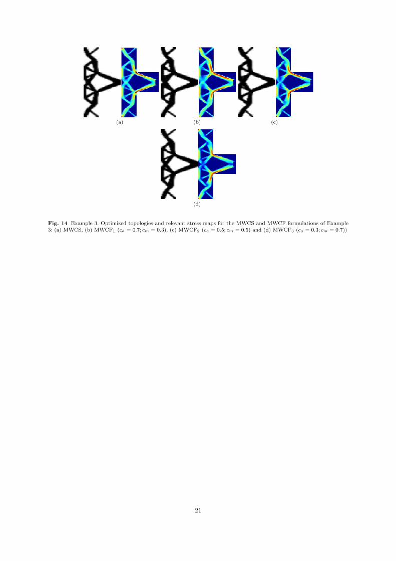
4.3 Example 3. The half–H lamina

For this third example, the design domain of Fig-

ure 3(c) is considered, loaded by a vertical force

P = 1, 667N . Once again, the solution of the strength–

constrained MWCS problem and the three ver-

sions of the fatigue–constrained problem are inves-

tigated. The relevant layouts and stress maps are

given in Figure 14(a) for the reference solution and

in Figures 14(b), 14(c) and 14(d) for the MWCF1,

MWCF2 and MWCF3 problems, respectively.

This last example confirms conclusion from the

two previous benchmarks. The optimal layouts found

by the considered optimization problems are along

the lines of the previous results: the members of the

structures achieved through fatigue–based proce-

dures are thicker than those of the reference one,

leading to heavier structures, see Figure 15(a) andTable 1. Furthermore, looking at Figures 16(a) to

16(c), one can see that all the elements used to

approximate the design domain meet the expec-

tations regarding fatigue resistance, with most of

the points showing a safety factor much bigger

than unity. As seen for the L–shaped specimen

of Section 4.2, the fatigue–constrained design be-

comes very similar to the strength–constrained lay-

out when the mean component prevails on the al-

ternate component of the stress. As outlined for

the long cantilever of Section 4.1, slightly non–

symmetric layouts are expected in case of fatigue–

constrained optimization, due to the different shape

of the adopted Goodman diagram in the first quad-

rant σeqm > 0 and in the second one σeqm < 0.

This example also confirms that the computa-

tional cost for problems involving fatigue design

is generally higher with respect to the strength–

based framework. Indeed, the optimization has to

15

handle an increased number of constraints, see Fig-

ure 15(b) and especially the MWCF1 problem. When

the alternate component of the stress prevails on

the mean one, the CPU time noticeably increases

with respect to a strength–based problem enforc-

ing the symmetric von Mises criterion. This is con-

sistent with physical expectation, suggesting that

the alternating part is the most critical one.

5 Conclusions

Fatigue is a complex mode of failure that needs to

be considered in the early stage of the design of any

mechanical component to select appropriate topol-

ogy. However, in case of high number of cycles,

dynamic analysis can be replaced by a static one

and fatigue resistance can be preliminary enforced

through an intuitive design rule that consists in as-

sessing the feasibility of the stress regime through-

out the domain with respect to a prescribed crite-

rion.

A simplified approach has been proposed herein

to cope with the minimization of the weight of

linear elastic structures under local fatigue con-

straints and a global compliance enforcement. The

expected stiffness of the optimized design is pro-

vided by the global constraint, whereas a set of lo-

cal stress–based enforces the structural fatigue re-

sistance. The Sines method has been used to define

the equivalent mean and alternate stress in case of

2D and 3D problem depending on the invariants

of the stress tensor and its deviatoric part, respec-

tively. Hence, a modified Goodman fatigue crite-

rion has been implemented through the same for-malism needed to address compression–dependent

failure in materials following the Drucker–Prager

strength criterion, see Bruggi and Duysinx (2012).

The so–called singularity phenomenon is overcome

by the implementation of a suitable relaxation of

the equivalent stress measures related to fatigue

resistance.

As expected, fatigue–constrained optimal lay-

outs circumvent geometric singularities to avoid

the arising of any stress peak. Numerical examples

show that fatigue design generally calls for heav-

ier structures with respect to strength–based op-

timization for the von Mises criterion, thickening

suitable parts of the optimal layout. When the al-

ternating component of the stress prevails on the

mean one, the achieved optimal truss–like struc-

tures are quite different with respect to conven-

tional strength–based layouts, as explained by the

shape of the Goodman diagram. Also, the adopted

fatigue failure criterion is not symmetric with re-

spect to the sign of the mean value of the stress,

thus often leading to some minor asymmetry in the

optimal structure.

Referring to computational issues, it has been

found that the fatigue–constrained optimization

is more demanding than the strength–constrained

design. Indeed, the set of active local constraints

steering the optimizer towards the achievement of

stiff fatigue–resistant layouts strongly depends on

the amount of alternating and mean component of

the stress.

It must be remarked that the proposed ap-

proach is a simplified design tool that can im-

prove conventional compliance–based layouts with

respect to fatigue adopting a straightforward ex-

tension of available formulations for stress–constrained

topology optimization. Notwithstanding the lim-

ited accuracy affecting the evaluation of the stress

field within a topology optimization problem, the

achieved layouts can be usefully exploited by the

designer to get a preliminary insight and to ini-

tialize more accurate procedures of optimization

and analysis based e.g. on shape optimization, as

outlined in Section 1.

Acknowledgements Part of the work has been done whenthe first author was spending a research period at Politec-

nico di Milano. This author would like to acknowledge the

Belgian National Fund for Scientific research (FRIA) for itsfinancial support.

Bibliography

Andreassen E, Clausen A, Schevenels M, Lazarov BS,

Sigmund O (2011) Efficient topology optimization inMATLAB using 88 lines of code. Struct Multidiscip Op-

tim 43:1–16

Bendsøe M, Kikuchi N (1988) Generating optimal topolo-gies in structural design using a homogeneization me-

thod. Comp Meth Appl Mech Eng 71:197–224

Bendsøe M, Sigmund O (2003) Topology optimization -Theory, methods and applications, Springer, EUA, New

York

Bourdin B (2001) Filters in topology optimization. Int JNumer Methods Eng 50:2143-2158

Bruggi M (2008) On an alternative approach to stress

constraints relaxation in topology optimization. StructMultidiscip Optim 36:125–141

Bruggi M, Dusyinx P (2012) Topology optimization forminimum weight with compliance and stress con-

straints. Struct Multidisc Optim 46(3):369-384Bruggi M, Dusyinx P (2013) A stress–based approach to

the optimal design of structures with unilateral behav-ior of material or supports . Struct Multidisc Optim

46(3):369-384Budynas R.G, Nisbett J.K (2011) Shigley’s Mechanical En-

gineering Design, 9th edition New York: McGraw-Hill

16

Bruns TE, Tortorelli DA (2001) Topology optimization

of non–linear elastic structures and compliant mech-anisms. Comp Meth Appl Mech Eng 190:3443–3459

Cheng GD, Guo X (1997) ε–relaxed approach in topologyoptimization. Struct Optim 13: 258–266

Duysinx P, Bendsøe MP (1998) Topology optimization of

continuum structures with local stress constraints. IntJ Numer Methods Eng 43: 1453–1478

Duysinx P (1999) Topology optimization with different

stress limits in tension and compression, In:Proceedingsof the 3rd World Congress of Structural and Multidis-

ciplinary Optimization WCSMO3

Duysinx P, Sigmund O (1998) New developments in han-dling stress constraints in optimal material distribution.

7th Symposium on Multidisciplinary Analysis and Op-

timization AIAA–98–4906: 1501–1509Duysinx P, Van Miegroet L, Lemaire E, Bruls O, Bruyneel

M (2008) Topology and generalized shape optimiza-tion: why stress constraints are so importants ? Int

J.Simul.Multidisc.Des.Optim. 2:253–258

Eschenauer HA, Olhoff N (2001) Topology optimizationof continuum structures: A review. Appl Mech Rev

54:331–389.

Grunwald J, Schnack E(1997) A fatigue model for shapeoptimization. Structural Optimization 14:36-44

Guilherme CEM, Fonseca JSO (2007) Topology optimiza-

tion of continuum structures with epsilon-relaxed stressconstraints. In:Alves M, da Costa Mattos HS (eds) Solid

mechanics in Brazil, vol 1. ABCM, Rio de Janeiro, pp

239–250Holmberg E, Torstenfelt B, Klarbring A (2013) Stress con-

strained topology optimization. Struc Multidisc Optim48:33– 47

Holmberg E, Torstenfelt B, Klarbring A (2014) Fatigue con-

strained topology optimization. Struc Multidisc Optim50:207– 219

Kaya N, Karen I, Ozturk F (2010) Re-design of a failed

clutch fork using topology and shape optimization bythe response surface method. Materials and Design

31:3008–3014

Kim Y.I, Park G.J (2010) Nonlinear dynamic responsestructural optimization using equivalent static loads.

Comput. Methods Appl. Mech. Engrg. 199:660–676

Kirsch U (1990) On singular topologies in optimal struc-tural design. Struct Optim 2:133–142

C. Lalanne (1999) Mechanical vibration & shock. VolumeIV, Fatigue damage. Hermes Penton Science, 1999.19

Le C, Norato J, Bruns TE, Ha C and Tortorelli DA

(2010) Stress–based Topology Optimization for Con-tinua. Struct Multidiscip Optim 41:605–620

Luo Y, Yu Wang Yu M, Kang Z (2013) An enhanced ag-

gregation method for topology optimization with localstress constraints. Comput. Method Appl. Mech. En-

grg. 254:31– 41Mrzygold M, Zielinski A.P 2006) Numerical implementa-

tion of multiaxial high-cycle fatigue criterion to struc-tural optimization. Journal of Theoretical and Applied

Mechanics, 44(3),pp 691–712Norton R. L (2000). Machine design: An integrated ap-

proach. Upper Saddle River, N.J: Prentice HallParıs J, Navarrina F, Colominas I, Casteleiro M (2009)

Topology optimization of continuum structures with lo-cal and global stress constraints. Struct Multidisc Op-tim 39(4):419–437

Park G.J, Kang B.S (2003)Validation of a structural op-

timisation algorithm transforming dynamic loads intoequivalent static loads. Journal of optimization theory

and applications: Vol 118, No.1., pp.191–200

Pereira JT, Fancello EA, Barcellos CS (2004) Topology op-timization of continuum structures with material failure

constraints. Struct Multidisc Optim 26(1–2):50–66

Rozvany GIN (2009) A critical review of established meth-ods of structural topology optimization. Struct Multi-

discip Optim 37:217–237

Seung H.J, Dong-Hoon C, Yoon G.H (2015) Fatigue andstatic failure considerations using topology optimiza-

tion method. Applied Mathematical Modeling 39:1137

– 1162Sherif K. and Irschik H. (2010) Efficient Topology Opti-

mization of Large Dynamic Finite Element Systems Us-ing Fatigue. AIAA Journal vol.48, No.7, pp 1339–1347

Schutz W. (1996) A history of fatigue Engineering Fracture

Mechanics Vol. 54, No. 2, pp. 263–300Sigmund O (2007) Morphology-based black and white fil-

ters for topology optimization. Structural and Multi-

disciplinary Optimization 33(4-5):401–424Sigmund O, Petersson J (1998) Numerical instabilities in

topology optimization: a survey on procedures dealing

with checkerboards, mesh-dependencies and local min-ima. Struct Optim 16:68–75

Svanberg K (1987) Method of moving asymptotes - A new

method for structural optimization. Int J Numer Meth-ods Eng 24:359–373

Svanberg K, Werme M (2007) Sequential integer program-

ming methods for stress constrained topology optimiza-tion. Struct Multidisc Optim 34(4):277–299

Svard H (2015) Topology Optimization of Fatigue-Constrained Structures, Doctoral Thesis, KTH Engi-

neering Sciences, Stockholm, Sweden

Svard H.(2015) Interior value extrapolation: a new me-thod for stress, evaluation during topology optimiza-

tion, Struct Multidisc Optim 51:613–629

Sved G, Ginos Z (1968) Structural optimization under mul-tiple loading. Int J Mech Sci 10:803–805

Yang RJ, Chen CJ (1996) Stress-based topology optimiza-

tion. Struct Multidisc Optim 12(2):98–105Weibull W. A statistical theory of the strength of materi-

als. Ingeniorsvetenskapsakademiens handlingar. Gener-

alstabens litografiska anstalts forlag, 1939.

17

(a)

(b)

(c)

Fig. 8 Comparison of the evolution of the objective func-tion (a), the number of active constraints (b) and the CPU

requirement (c) for the three strategies of example 2

18

(a) (b)

Fig. 11 Comparison of MWF1 and MWCF1 problems: a) Objective function b) CPU times

(a) (*) (b)

Fig. 12 Comparison of MWCF1 for real and fictious material properties: a) ca = 0, 7 and cm = 0, 3 (∗ stands for real

material) b) ca = 0, 7 and cm = 0, 3 and αc = 2

19

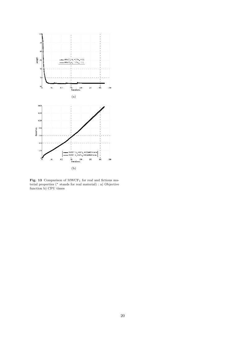
(a)

(b)

Fig. 13 Comparison of MWCF1 for real and fictious ma-

terial properties (∗ stands for real material) : a) Objectivefunction b) CPU times

20

(a) (b) (c)

(d)

Fig. 14 Example 3. Optimized topologies and relevant stress maps for the MWCS and MWCF formulations of Example

3: (a) MWCS, (b) MWCF1 (ca = 0.7; cm = 0.3), (c) MWCF2 (ca = 0.5; cm = 0.5) and (d) MWCF3 (ca = 0.3; cm = 0.7))

21

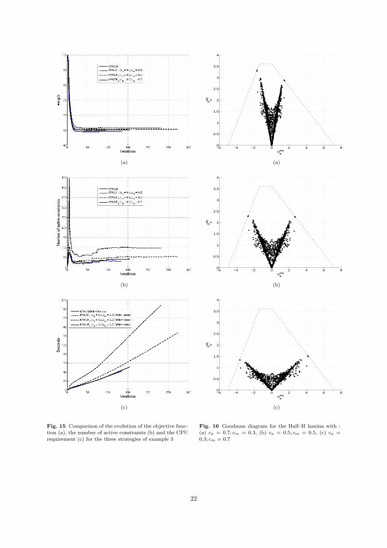
(a)

(b)

(c)

Fig. 15 Comparison of the evolution of the objective func-tion (a), the number of active constraints (b) and the CPU

requirement (c) for the three strategies of example 3

−6 −4 −2 0 2 4 6 80

0.5

1

1.5

2

2.5

3

3.5

4

σmeq

σ aeq

(a)

−6 −4 −2 0 2 4 6 80

0.5

1

1.5

2

2.5

3

3.5

4

σmeq

σ aeq

(b)

−6 −4 −2 0 2 4 6 80

0.5

1

1.5

2

2.5

3

3.5

4

σmeq

σ aeq

(c)

Fig. 16 Goodman diagram for the Half–H lamina with :(a) ca = 0.7; cm = 0.3, (b) ca = 0.5; cm = 0.5, (c) ca =

0.3; cm = 0.7

22