Embed Size (px)
Citation preview
MINIMUM WEIGHT TOPOLOGY OPTIMIZATION SUBJECT TO
UNSTEADY HEAT EQUATION AND SPACE-TIME POINTWISE
CONSTRAINTS – TOWARD AUTOMATIC OPTIMAL RISER
DESIGN IN THE SHAPE CASTING PROCESS
R. TAVAKOLI
Abstract. The automatic optimal design of feeding system in the shape cast-
ing process is considered, i.e., to find the optimal position, size, shape and
topology of risers, and riser-necks. It is formulated as a minimum weighttopology optimization problem subjected to a nonlinear transient PDE and
an infinite number of space-time pointwise constraints. In addition to regular-
ization and relaxation of the original model, an elegant bilevel reformulationof the optimization problem is introduced which makes it possible to man-
age the infinite number of design parameters and state-constraints efficiently.
The computational cost of this method is asymptotically independent from thenumber of design parameters and constraints. The validity and efficiency of
the presented method are supported by several examples, from simple bench-marks to complex industrial castings. According to our numerical results, the
presented approach makes a relatively complete solution to the problem of
automatic optimal rider design in the shape casting process.
Keywords. adjoint sensitivity, feeder design, homogenization, Niyama crite-rion, pointwise constraints, projected gradient, regularization, relaxation.
Contents
1. Introduction 22. Conceptual modeling 23. Mathematical modeling 54. Regularization of the mathematical model 95. Relaxation of the mathematical model 116. SIMP penalization of mathematical model 127. Bilevel reformulation of the optimization problem 138. Necessary optimality conditions for the lower-level problem 199. Projection onto the admissible control domain 2510. Numerical method 2911. Numerical results 3012. Summary 42Acknowledgment 42References 43
Date: May 13, 2011.Rouhollah Tavakoli, Department of Material Science and Engineering, Sharif University of
Technology, Tehran, Iran, P.O. Box 11365-9466, [email protected].
1
2 R. TAVAKOLI
1. Introduction
Metal casting is an important process to produce near net-shape products, whichare used extensively in automotive and aerospace industries. Since metals usuallycontrast on the solidification, the last freezing points in castings encounter the lackof molten metal. If this leakage is not compensated properly, it leaves some shrink-age porosities in either of macroscopic or microscopic form within the castings.Risers are appended to the castings to establish the directional solidification fromthe casting to the risers so that the final solidification points are located within therisers. They are cut-off and recycled after the solidification. The goal of an optimalriser design procedure is to find the locations, sizes and shapes of risers. Moreover,the total weight of risers should be minimized to improve the casting yield and pro-ductivity. The goal of this paper is to introduce a method for automatic optimalriser design in the shape casting process.
Although methods for the product design optimization are well documented inliterature (cf. [6]), the process design optimization, in particular in the field ofriser design, has received less attention in spite of its importance. The remarkablestudies in this regard have been carried out by Daniel Tortorelli et. al. in theuniversity of Illinois-Urbana (cf. [31]) and Roland Lewis et. al. in the universityof Wales-Swansea (cf. [20]). In these works, the optimization of riser design is for-mulated as a parametric shape optimization problem which is solved by a gradientbased minimization method. The objective function to be minimized is defined asthe riser volume and a few constraints are defined to enforce the directional solid-ification along a priori-defined feeding path. Two important prerequisites of thesemethods are a nearly feasible initial design and a user defined feeding path. Theseprerequisites make this approach far from our ultimate goal which is the automaticoptimal riser design in the shape casting process.
The goal of present study is to introduce a mathematical model and its cor-responding numerical method to automate the above mentioned optimal designproblem. It can be accounted as a follow up part of our early work (see: [28]) inthis regard.
The main contributions of the present work can be listed as follows: the mathe-matical formulation of a sophisticated engineering design problem in the frameworkof topology optimization; the space-time regularization of non-smooth PDEs andfunctionals; introducing a continuous solution strategy to efficiently manage theinfinite number of control parameters and state-dependent pointwise constraints;introducing an efficient method for the projection onto a design space formed bythe integral and bound constraints; suggesting some new riser design rules basedon numerical results.
2. Conceptual modeling
The selection of design parameters is the first step of every optimal design prob-lem. In previous works (see: [20, 31]) the shape parameters of riser(s) are consideredas the design parameters. The small number of design parameters is the main ben-efit of this approach. However, it is not able to change the topology of feedingsystem. Moreover, it needs an appropriate initial design and a user defined feedingpath. To overcome these limitations, the topology optimization approach (cf. [6])is adapted in the present study. It is originally developed for the optimal designof macro or micro mechanical structures. In this method, the topology indicator
AUTOMATIC OPTIMAL RISER DESIGN 3
function at each spatial point is defined as the design parameters. Therefore, thereare an infinite number of design parameters, before the spatial discretization.
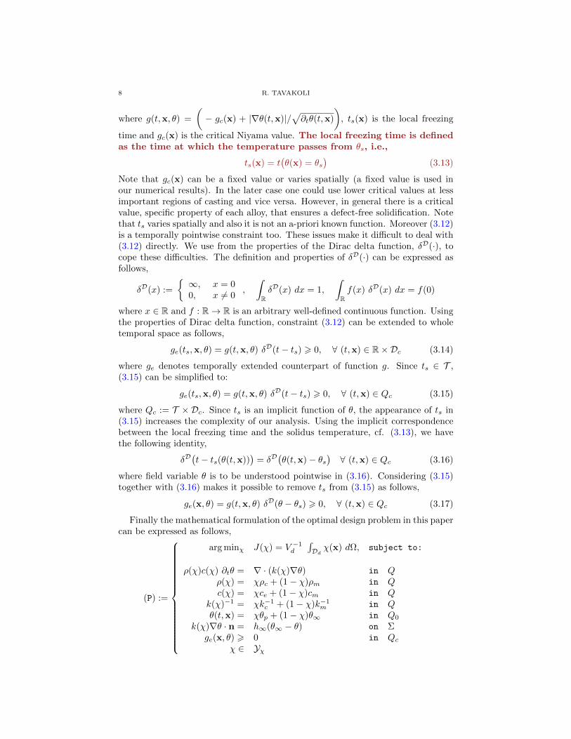
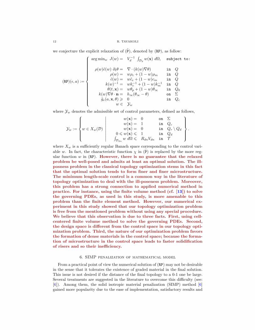
Without loss of generality, the physical domain, D ⊂ R3, is assumed to berectangular, i.e., D = [0, lx]× [0, ly]× [0, lz]. In practice, D is identical to mold-boxin the shape casting process. Henceforth, the global spatial domain is called as themold-box in this study. The original casting, denoted by Dc ⊂ D, is consideredas an embedded object within the mold-box. The topology indicator function isequal to unity within Dc. It will be remained constant inside Dc during the optimaldesign procedure. The location of casting in D and lx, ly, lz should be selected sothat there will be sufficient space within the mold-box to design an appropriablefeeding system. Excluding Dc from D, the remainder of mold-box is denoted byDr, i.e., Dr = D \ Dc. The design space of feeding system, Dd, is a subset of Dr,i.e., Dd ⊆ Dr. In a worse condition Dd is identical to Dr. However it is preferredto restrict Dd, excluding portions of Dr which are not suitable for the design offeeding system. For instance, one can excludes bottom portions of the mold-boxfrom Dd. In our method, Dd is decomposed into two (open) sub-domainsDdr and Ddn such that Dd = Ddr ∪ Ddn and Ddr ∩ Ddn = Γrn. Ddr and Ddnrespectively denote the riser and riser-neck1design domains. Γrn denotesthe boundary between Ddr and Ddn. In practice Ddn is a shell of Dd around thecast part with thickness ln. To improve the quality of the final design, the user canexclude infeasible portions of Dd from Ddn. For instance, the connection of risersto high curvature and bottom surfaces is discouraged. The above mentioned designdomains are schematically shown in figure 1. The topology indicator function is
D Dc Dr
Dd Ddn Ddr
Figure 1. Schematic of spatial domains D, Dc, Dr Dd, Ddn andDdr defined in this study (shaded regions).
equal to zero inside Dr \(Ddn∪Ddr) and will be fixed there during the optimization.
1Since riser(s) should be separated from the casting after the solidification, the connection areaof riser to the casting, called as the riser-neck, should be minimal to reduce the machining cost.
4 R. TAVAKOLI
It varies inside Ddn and Ddr during the optimization. It assumes the value of eitherunity or zero within these regions which is equivalent to existence of metal and moldmaterials respectively. In fact, our goal is to determine the optimal value of thetopology indicator field inside Ddn ∪Ddr such that its corresponding design resultsa defect free casting. Moreover, to optimize the casting yield the minimization ofthe total value of metal phase inside Dd is desired. Assume that the volume ofDd, Ddr and Ddn are denoted by Vd, Vdr and Vdn respectively. For the purpose ofriser-neck design, the total volume fraction of metal phase, denoted by Rdn, insideDdn is constrained by an upper bound value.
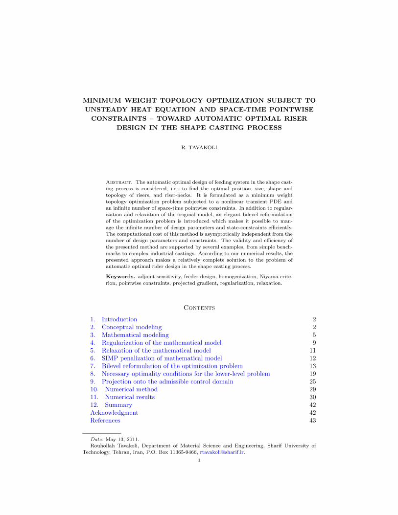
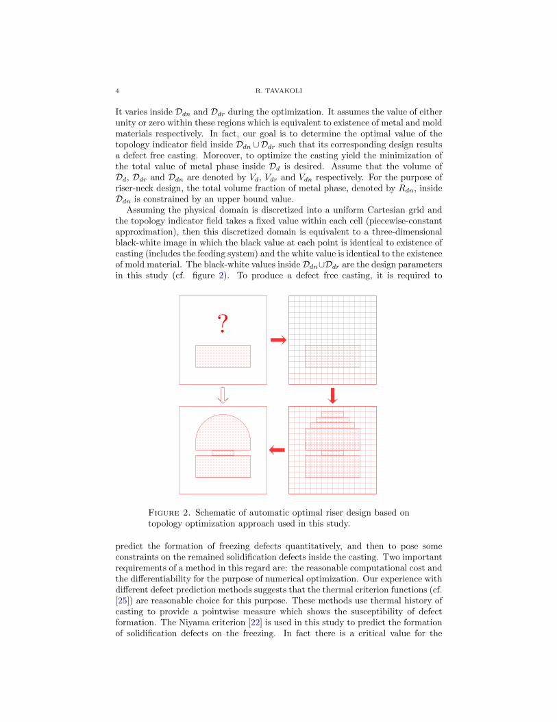
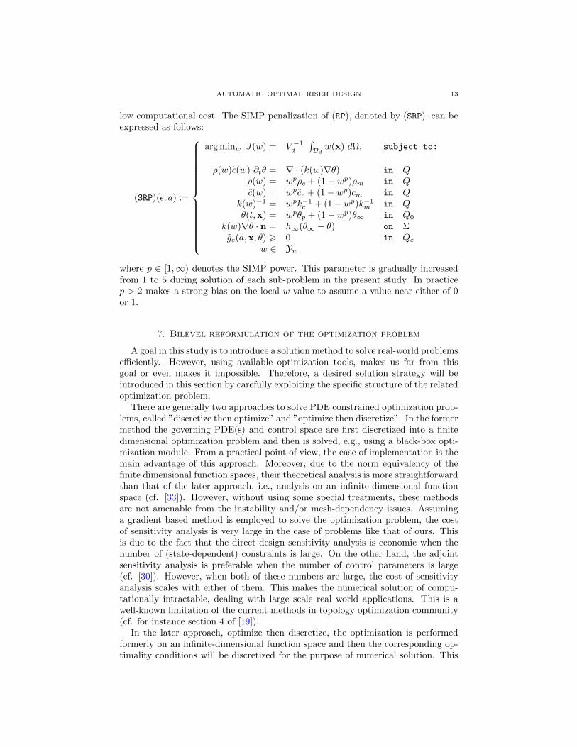
Assuming the physical domain is discretized into a uniform Cartesian grid andthe topology indicator field takes a fixed value within each cell (piecewise-constantapproximation), then this discretized domain is equivalent to a three-dimensionalblack-white image in which the black value at each point is identical to existence ofcasting (includes the feeding system) and the white value is identical to the existenceof mold material. The black-white values inside Ddn∪Ddr are the design parametersin this study (cf. figure 2). To produce a defect free casting, it is required to
?
Figure 2. Schematic of automatic optimal riser design based ontopology optimization approach used in this study.
predict the formation of freezing defects quantitatively, and then to pose someconstraints on the remained solidification defects inside the casting. Two importantrequirements of a method in this regard are: the reasonable computational cost andthe differentiability for the purpose of numerical optimization. Our experience withdifferent defect prediction methods suggests that the thermal criterion functions (cf.[25]) are reasonable choice for this purpose. These methods use thermal history ofcasting to provide a pointwise measure which shows the susceptibility of defectformation. The Niyama criterion [22] is used in this study to predict the formationof solidification defects on the freezing. In fact there is a critical value for the
AUTOMATIC OPTIMAL RISER DESIGN 5
Niyama criterion so that regions of casting with lower Niyama value are suspectableto include shrinkage defects [22]. It is important to note that the Niyama criterionat each point should be evaluated at the local freezing time. Therefore, we will havean infinite number of space-time pointwise constraints, to be satisfied, to producea sound casting.
Considering the Niyama criterion to predict the solidification defects, we haveto make the following assumptions in this study:
(H1) The mold cavity is already filled with the molten metal and the tempera-ture distribution is a-priori known (e.g. considering a uniform temperaturedistribution for the purpose of convenience).
(H2) The effect of the gravity on the solidification is ignored.(H3) The solidification interval, the difference between the liquidus and solidus
temperatures, is sufficiently small. In fact we have a narrow-bound freezingwhich possesses a nearly planar macroscopic solid-liquid interface.
(H4) The melt has a good metallurgical quality such that the solidification defectstend to appear as macro-shrinkages.
Without loss of generality, the following assumptions are made to avoid extra com-plexity and computational cost:
(H5) The effect of alloying elements segregation on the solidification is ignored.This assumption is particularly reasonable in the case of carbon steels.
(H6) The effect of air-gap formation2 during the solidification is ignored. This isa reasonable assumption particularly in the case of sand casting process.
(H7) The heat transfer coefficient on the cast-mold interface within the designdomain is computed using the harmonic averaging. This assumption alsoworks well in the case of sand-mold casting.
(H8) The latent heat of solidification is linearly distributed within the freezinginterval. This is reasonable assumption almost for every alloying system, inparticular whenever there is no explicit relation between the solid fractionand temperature (cf. [16]).
In addition to the above mentioned constraints, some geometric constraintsshould be taken into account to ensure the moldability of the final design (cf.[11]). However , the moldability constraints are not considered in the present study.Hopefully, this issue will be considered in our forthcoming work.
3. Mathematical modeling
The presented model in the previous section will be expressed in the mathe-matical language here. Ignoring the effect of melt flow during the solidification,the temperature history of casting can be modeled by the following nonlinear heattransfer equation (cf. [16]):
ρc(θ)cc(θ) ∂tθ = ∇ · (kc(θ)∇θ) + ρc(θ)L∂tfs in T × Dmρm(θ)cm(θ) ∂tθ = ∇ · (km(θ)∇θ) in T × D \ Dmθ(t,x) = θ0(x) in t = 0 × D−km∇θ · n = h∞(θ − θ∞) on T × ∂Dki∇θ · ni |cast = −ki∇θ · ni |mold on T × ∂Dm
(3.1)
2In practice air-gap forms at the cast-mold interface due to the simultaneous contraction ofthe solidified skin and expansion of the mold walls.
6 R. TAVAKOLI
where T := (0, T ] denotes the temporal domain (T is sufficiently large to capturethe whole dynamics of solidification), ∂t(·) denotes the partial derivatives respectto the temporal coordinate, Dm ⊂ D is a portion of the mold-box which is occupiedby the metal phase, i.e., the casting and the corresponding feeding system, θ isthe temperature, ρ is the density, c is the specific heat capacity, k is the thermalconductivity, L is the fusion latent heat, fs is the local solid fraction, θ0 is the initialtemperature distribution, h∞ is the air-mold interfacial heat transfer coefficient,θ∞ is the ambient temperature, n is outer unit normal on ∂D, ki is the cast-moldinterfacial heat transfer coefficient, ni is unit normal on ∂Dm directed toward themold and subscripts (·)c and (·)m denotes the metal and mold materials respectively.As it was explained before (assumption H7), ki is computed through the harmonicaveraging as follows:
k−1i =
(k−1c + k−1
m
)/2 (3.2)
Note that in practice, we have the discontinuity of heat flux at the cast-mold interface and assumption H7 does not hold in general. However,due to low conductivity of sand mold, the continuity of heat flux at thecast-sand interface is a reasonable simplification. Moreover, we have toemploy this assumption in this study to homogenize the governing equa-tion required for the purpose of topology optimization. Furthermore,the choice of harmonic mean, instead of arithmetic mean, is based onVoller work [34] in which it was shown that for rapidly changing heatconductivity, the harmonic averaging leads to more accurate results thanthose of the arithmetic averaging. In fact, in this way the cast and molddomain are contrasted by mathematical model implicitly through therapid change in physical properties.
It is assumed that at t = 0, the temperature is uniform within the mold and isequal to the ambient temperature. The casting temperature is also assumed to beequal to the pouring temperature, θp, i.e.,
θ0(x) =
θp, in Dmθ∞, elsewhere
(3.3)
Without lose of generality, in order to improve the computational performance, itis assumed that the physical properties are temperature invariant. This assumptionsimplifies, (3.1) into the following form:
ρccc ∂tθ = ∇ · (kc∇θ) + ρcL∂tfs in T × Dmρmcm ∂t = ∇ · (km∇θ) in T × D \ Dmθ(t,x) = θ0(x) in t = 0 × D−km∇θ · n = h∞(θ − θ∞) on T × ∂Dki∇θ · ni |cast = −ki∇θ · ni |mold on T × Γi
(3.4)
Assume that the solidus and liquidus temperatures are denoted by θs and θl re-spectively, using assumption (H8) in the previous section results:
fs(θ) =
0, θ > θl(θl − θ)/(θl − θs), θs 6 θ 6 θl1, θ < θs
(3.5)
AUTOMATIC OPTIMAL RISER DESIGN 7
therefore,
∂fs(θ)
∂θ=
0, θ > θl(θs − θl)−1, θs < θ < θl0, θ < θs
(3.6)
notice that fs(θ) is not differentiable at θ = θs and θ = θl. This issue is temporaryignored here. This problem will be fixed later in section 4. According to chain rulewe have: ∂fs/∂t = (∂fs/∂T )(∂T/∂t). Therefore, considering (3.4) together with(3.6) results:
ρcce(θ) ∂tθ = ∇ · (kc∇θ) in T × Dmρmcm ∂tθ = ∇ · (km∇θ) in T × D \ Dmθ(t,x) = θ0(x) in t = 0 × D−km∇θ · n = h∞(θ − θ∞) on T × ∂Dki∇θ · ni |cast = −ki∇θ · ni |mold on T × Γi
(3.7)
where the effective specific heat capacity, denoted by ce, is computed as follows:
ce(θ) =
cc, θ > θlcc + L(θl − θs)−1, θs < θ < θlcc, θ < θs
(3.8)
As it is discussed in section 2, the topology indicator function, χ, inside Dd is thedesign parameter in this study. In fact this function is the characteristic functionof the metal phase within D, i.e.:
χ(x) :=
1, in Dm0, elsewhere
(3.9)
Since function χ(x) varies during our optimization, the solution domain in (3.7)should be varied accordingly. Using (3.9), we can rewrite (3.7) in the followingform:
ρ(χ)c(χ) ∂tθ = ∇ · (k(χ)∇θ) in Qρ(χ) = χρc + (1− χ)ρm in Qc(χ) = χce + (1− χ)cm in Qk(χ)−1 = χk−1
c + (1− χ)k−1m in Q
θ(t,x) = χθp + (1− χ)θ∞ in Q0
k(χ)∇θ · n = h∞(θ∞ − θ) on Σ
(3.10)
where Q := T ×D, Q0 := t = 0 ×D, Σ := T × ∂D and it is assumed that χ onthe cast-mold interface is computed by a linear interpolation. It is easy to check
that for a fixed topology, (3.10) is equivalent to (3.7). In fact (3.10) automaticallyadapts the governing equations according to the current topology.
The objective function to be minimized in this study is defined as the scaledtotal volume of the molten metal used in the design domain, i.e.,
arg minχ∈0,1
J(χ) = V −1d
∫Ddχ(x) dΩ (3.11)
where dΩ denotes the volume measure induced in D.As it is discussed in section 2, the space-time pointwise value of the Niyama
criterion is constrained in Dc to ensure the production of a defect-free casting.Therefore, our state-dependent constraints can be expressed in the following form(cf. [22, 25] for further details about the Niyama criterion),
g(t = ts(x),x, θ
)> 0, ∀ x ∈ Dc (3.12)
8 R. TAVAKOLI
where g(t,x, θ) =
(− gc(x) + |∇θ(t,x)|/
√∂tθ(t,x)
), ts(x) is the local freezing
time and gc(x) is the critical Niyama value. The local freezing time is definedas the time at which the temperature passes from θs, i.e.,
ts(x) = t(θ(x) = θs
)(3.13)
Note that gc(x) can be a fixed value or varies spatially (a fixed value is used inour numerical results). In the later case one could use lower critical values at lessimportant regions of casting and vice versa. However, in general there is a criticalvalue, specific property of each alloy, that ensures a defect-free solidification. Notethat ts varies spatially and also it is not an a-priori known function. Moreover (3.12)is a temporally pointwise constraint too. These issues make it difficult to deal with(3.12) directly. We use from the properties of the Dirac delta function, δD(·), tocope these difficulties. The definition and properties of δD(·) can be expressed asfollows,
δD(x) :=
∞, x = 00, x 6= 0
,
∫RδD(x) dx = 1,
∫Rf(x) δD(x) dx = f(0)
where x ∈ R and f : R→ R is an arbitrary well-defined continuous function. Usingthe properties of Dirac delta function, constraint (3.12) can be extended to wholetemporal space as follows,
ge(ts,x, θ) = g(t,x, θ) δD(t− ts) > 0, ∀ (t,x) ∈ R×Dc (3.14)
where ge denotes temporally extended counterpart of function g. Since ts ∈ T ,(3.15) can be simplified to:
ge(ts,x, θ) = g(t,x, θ) δD(t− ts) > 0, ∀ (t,x) ∈ Qc (3.15)
where Qc := T × Dc. Since ts is an implicit function of θ, the appearance of ts in(3.15) increases the complexity of our analysis. Using the implicit correspondencebetween the local freezing time and the solidus temperature, cf. (3.13), we havethe following identity,
δD(t− ts(θ(t,x))
)= δD
(θ(t,x)− θs
)∀ (t,x) ∈ Qc (3.16)
where field variable θ is to be understood pointwise in (3.16). Considering (3.15)together with (3.16) makes it possible to remove ts from (3.15) as follows,
ge(x, θ) = g(t,x, θ) δD(θ − θs) > 0, ∀ (t,x) ∈ Qc (3.17)
Finally the mathematical formulation of the optimal design problem in this papercan be expressed as follows,
(P) :=
arg minχ J(χ) = V −1d
∫Dd χ(x) dΩ, subject to:
ρ(χ)c(χ) ∂tθ = ∇ · (k(χ)∇θ) in Qρ(χ) = χρc + (1− χ)ρm in Qc(χ) = χce + (1− χ)cm in Q
k(χ)−1 = χk−1c + (1− χ)k−1
m in Qθ(t,x) = χθp + (1− χ)θ∞ in Q0
k(χ)∇θ · n = h∞(θ∞ − θ) on Σge(x, θ) > 0 in Qc
χ ∈ Yχ
AUTOMATIC OPTIMAL RISER DESIGN 9
where Yχ denotes the admissible domain of the control variable which is defined asfollows,
Yχ :=
χ ∈ Xχ(D)
∣∣∣∣∣∣∣∣∣∣χ(x) = 0 on Σχ(x) = 1 in Qcχ(x) = 0 in Qr \Qdχ(x) ∈ 0, 1 in Qd∫
Ddn χ dΩ 6 RdnVdn in T
.
where Qr := T × Dr, Qd := T × Dd and Xχ denotes a function space with suffi-cient regularity required for characteristic functions in D. Note that the boundarycondition χ = 0 on the external boundaries of the mold box is applied in problem(P) to improve the convergence-rate during the numerical solution.
Remark 3.1. It should be noticed that the structure of topology optimization prob-lem (P) is different from the classical topology optimization problems in the sensethat the objective functional (or target) space is not identical to the control space.More precisely, in the classical topology optimization problems the optimal materi-als distribution is found within a spatial domain on which the objective functionaland constraints are defined. However, regarding to problem (P), the optimal mate-rial distribution is found within Dd to pose control inside Dc. In fact, a new classof topology optimization problems is introduced in the present study. This con-tribution hopefully increases the utility of topology optimization concept to solvemore class of engineering design problems.
Remark 3.2. There is a well-known problem called the flux or stress singularitywhich is usually connected to the topology optimization problems subject to point-wise gradient constraints (cf. [19]). This problem is mathematically equivalent tothe lack of constraint qualifications in the course of optimization. Using the com-bination of the mixed formulation and the phase-filed relaxation, a mathematicallyrigorous solution to this problem is introduced in [10]. Moreover, several heuristicsolutions are suggested in engineering literature (see: [19] and references therein).Because the topology of Dc is fixed during the optimization in the present study,our mathematical model is free from the mentioned problem.
4. Regularization of the mathematical model
As it was warned in section 3, fs(θ) in equation (3.5) (and so ce(θ)) is notdifferentiable at θ = θs and θ = θl. We can express (3.5) in the following equivalentform,
fs(θ) = (θs − θl)−1(H(θ − θs)−H(θ − θl)
)(4.1)
where H(x) : R → R denotes the one-dimensional Heaviside function which isdefined as follows (cf. chapter 1 of [23]):
H(x) :=
0, x < 01, x > 0
(4.2)
Following [23], the smoothed form of the one-dimensional Heaviside function canbe expressed as follows,
Hε(x) =
0, x < −ε12 + x
2ε + 12π sin
(πxε
), −ε 6 x 6 ε
1, x > ε(4.3)
10 R. TAVAKOLI
where ε ∈ (0,∞) is the smoothing parameter in the sense that: H(x) = limε→0 Hε(x).
It is clear that H is a C2 function. Using the smoothed one-dimensional Heavisidefunction (4.4) can be rewritten as follows:
fs(θ) = (θs − θl)−1(Hε(θ − θs)− Hε(θ − θl)
)(4.4)
where fs denotes the regularized solid fraction function. Similarly, the regularizedeffective specific heat capacity function, ce, can be expressed as follows:
ce = cc + L (θl − θs)−1(Hε(θ − θs)− Hε(θ − θl)
)(4.5)
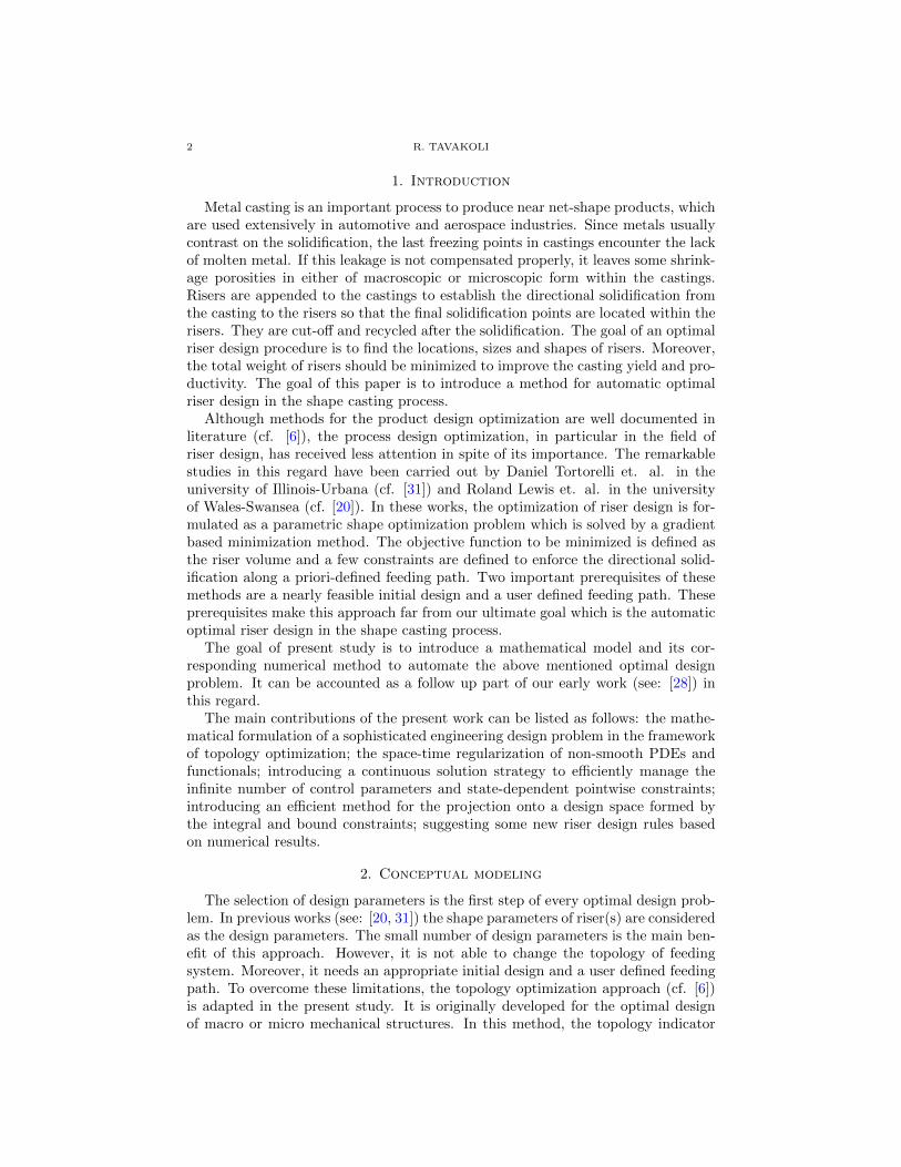
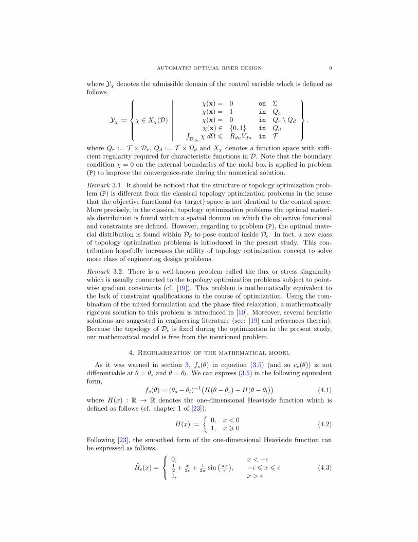
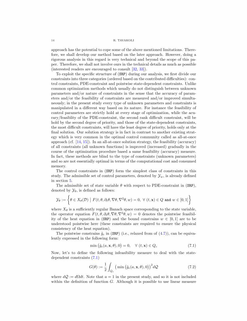
The graph of ce and ce functions are schematically shown in figure 3.
θs θlθ
ce, ce
cc
cc +L
θl−θs
2ε
ce
ce
Figure 3. Schematic plots of ce and ce functions in the presentstudy. The regularization parameter in smoothed Heaviside func-tion is equal to one-tenth of the freezing range in this plot, i.e.,ε = 0.1(θl − θs).
Note that we do not solve the ε-decreasing sequence of problems in practice, butonly solve a problem with a sufficiently small smoothing parameter. The appliedsmoothing parameter in this study is equal to one-tenth of the freezing interval,i.e., ε = 0.1(θl − θs).
The presence of the Dirac delta function in constraints (3.17) leads to somedifficulties in both of the sensitivity analysis due to the differentiability issue andthe numerical solution due to the concentration of function at (a-priori) unknowntime. To overcome these problems, the Dirac delta function is regularized in thisstudy. The regularized Dirac delta function, δDa (x) : R→ R, is a sufficiently smoothfunction such that (cf. [1]):∫
RδDa (x) dx = 1, δD(x) = lim
a→0δDa (x)
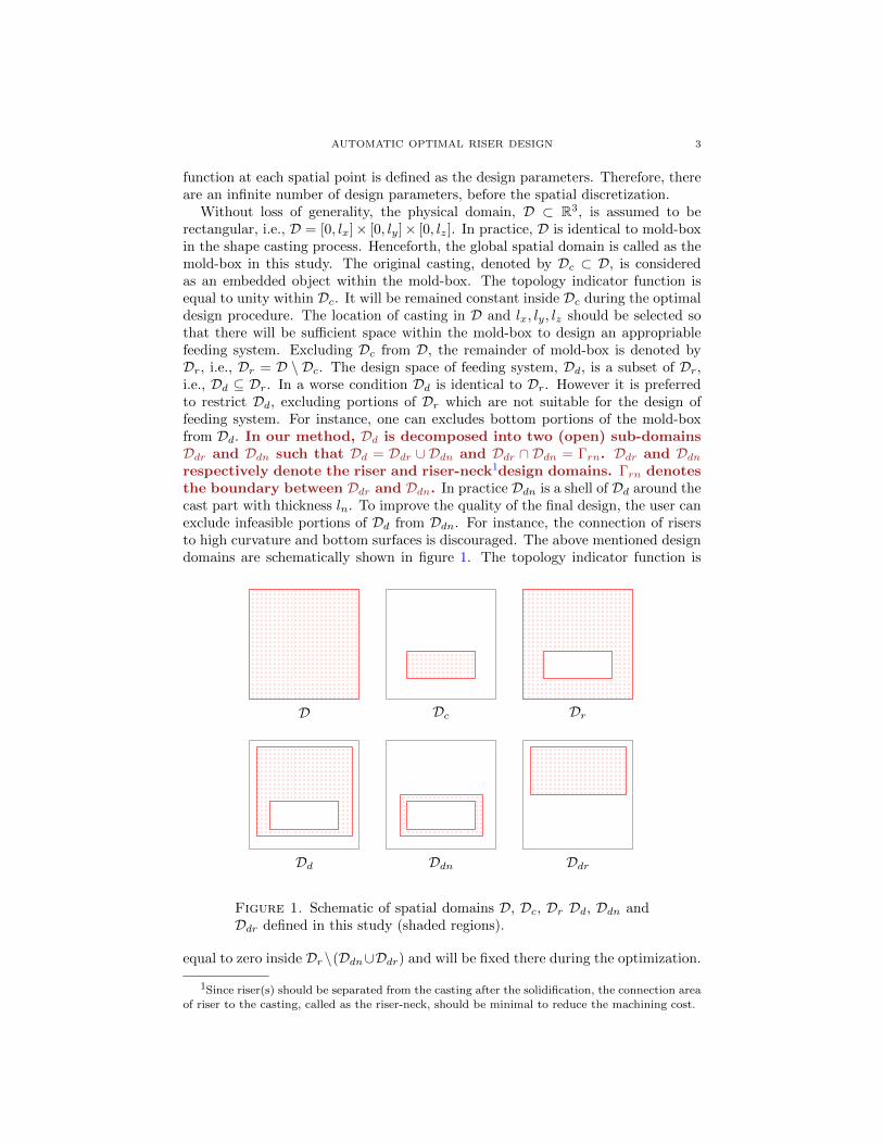
where a ∈ (0,∞) is regularization parameter which controls the intensity of smooth-ing. The bell-shaped probability density function is used as the regularized coun-terpart of the Dirac delta function in this study. Therefore, by δDa (x) we denotethe following function henceforth:
δDa (x) =1
a√
2πe−(x)2/(2a2) (4.6)
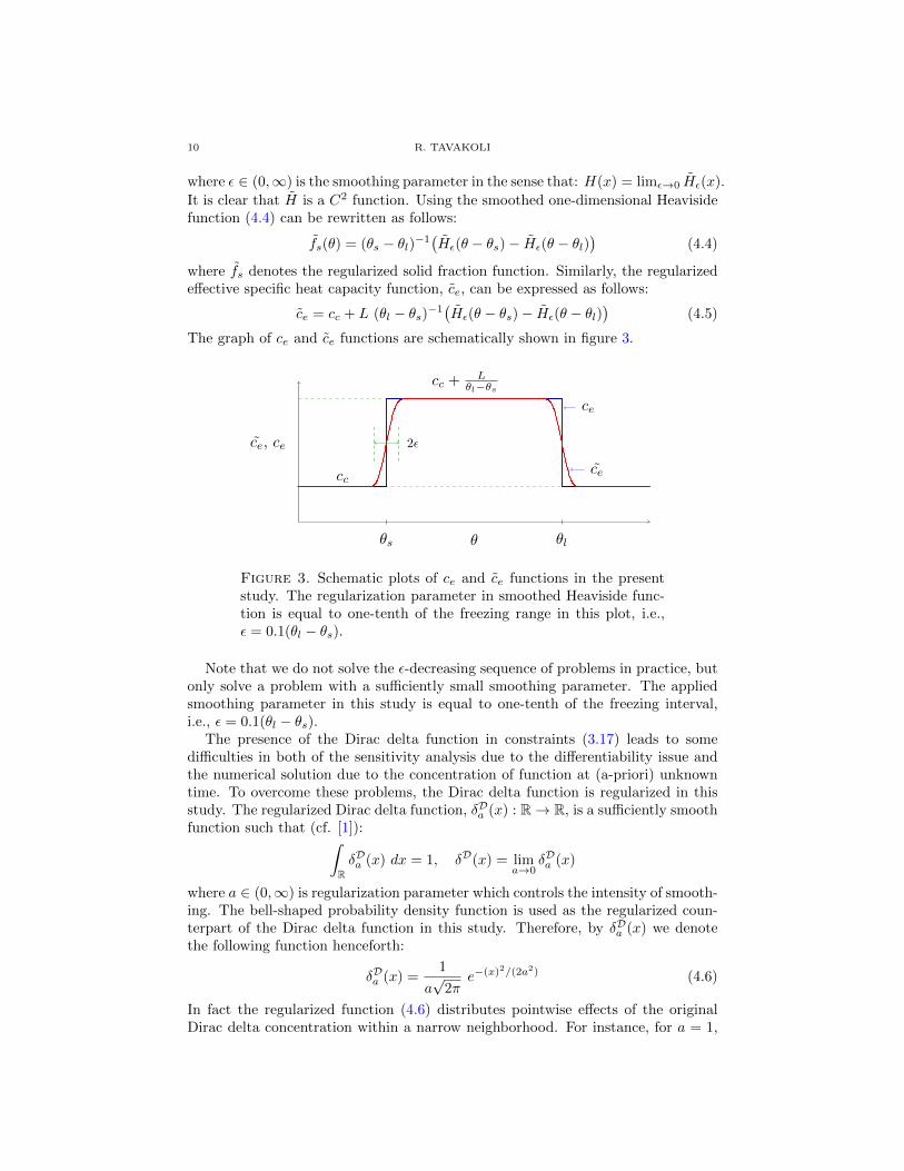
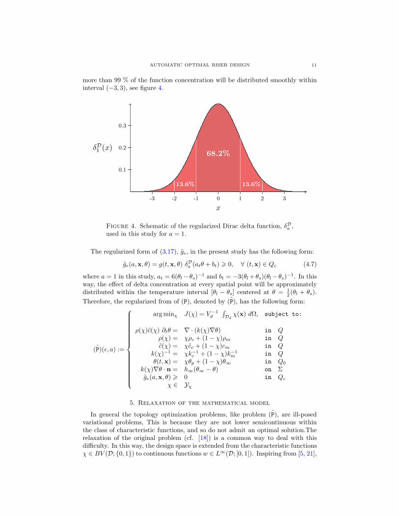
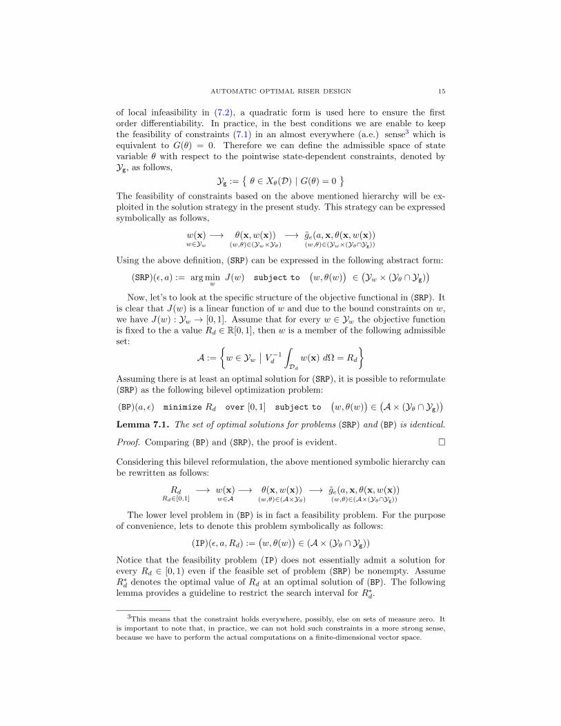
In fact the regularized function (4.6) distributes pointwise effects of the originalDirac delta concentration within a narrow neighborhood. For instance, for a = 1,
AUTOMATIC OPTIMAL RISER DESIGN 11
more than 99 % of the function concentration will be distributed smoothly withininterval (−3, 3), see figure 4.
0.1
0.2
0.3
δD1 (x)
-3 -2 -1 0 1 2 3
x
68.2%
13.6% 13.6%
Figure 4. Schematic of the regularized Dirac delta function, δDa ,used in this study for a = 1.
The regularized form of (3.17), ge, in the present study has the following form:
ge(a,x, θ) = g(t,x, θ) δDa (atθ + bt) > 0, ∀ (t,x) ∈ Qc (4.7)
where a = 1 in this study, at = 6(θl− θs)−1 and bt = −3(θl+ θs)(θl− θs)−1. In thisway, the effect of delta concentration at every spatial point will be approximatelydistributed within the temperature interval [θl − θs] centered at θ = 1
2 (θl + θs).
Therefore, the regularized from of (P), denoted by ˜(P), has the following form:
˜(P)(ε, a) :=
arg minχ J(χ) = V −1d
∫Dd χ(x) dΩ, subject to:
ρ(χ)c(χ) ∂tθ = ∇ · (k(χ)∇θ) in Qρ(χ) = χρc + (1− χ)ρm in Qc(χ) = χce + (1− χ)cm in Q
k(χ)−1 = χk−1c + (1− χ)k−1
m in Qθ(t,x) = χθp + (1− χ)θ∞ in Q0
k(χ)∇θ · n = h∞(θ∞ − θ) on Σge(a,x, θ) > 0 in Qc
χ ∈ Yχ
5. Relaxation of the mathematical model
In general the topology optimization problems, like problem ˜(P), are ill-posedvariational problems, This is because they are not lower semicontinuous withinthe class of characteristic functions, and so do not admit an optimal solution.Therelaxation of the original problem (cf. [18]) is a common way to deal with thisdifficulty. In this way, the design space is extended from the characteristic functionsχ ∈ BV (D; 0, 1) to continuous functions w ∈ L∞(D; [0, 1]). Inspiring from [5, 21],
12 R. TAVAKOLI
we conjecture the explicit relaxation of ˜(P), denoted by (RP), as follow:
(RP)(ε, a) :=
arg minw J(w) = V −1d
∫Dd w(x) dΩ, subject to:
ρ(w)c(w) ∂tθ = ∇ · (k(w)∇θ) in Qρ(w) = wρc + (1− w)ρm in Qc(w) = wce + (1− w)cm in Q
k(w)−1 = wk−1c + (1− w)k−1
m in Qθ(t,x) = wθp + (1− w)θ∞ in Q0
k(w)∇θ · n = h∞(θ∞ − θ) on Σge(a,x, θ) > 0 in Qc
w ∈ Ywwhere Yw denotes the admissible set of control parameters, defined as follows,
Yw :=
w ∈ Xw(D)
∣∣∣∣∣∣∣∣∣∣w(x) = 0 on Σw(x) = 1 in Qcw(x) = 0 in Qr \Qd
0 6 w(x) 6 1 in Qd∫Ddn w dΩ 6 RdnVdn in T
.
where Xw is a sufficiently regular Banach space corresponding to the control vari-
able w. In fact, the characteristic function χ in ˜(P) is replaced by the more reg-ular function w in (RP). However, there is no guarantee that the relaxedproblem be well-posed and admits at least an optimal solution. The ill-posness problem in the classical topology optimization stems in this factthat the optimal solution tends to form finer and finer microstructure.The minimum length-scale control is a common way in the literature oftopology optimization to deal with the ill-poseness problem. Moreover,this problem has a strong connection to applied numerical method inpractice. For instance, using the finite volume method (cf. [13]) to solvethe governing PDEs, as used in this study, is more amenable to thisproblem than the finite element method. However, our numerical ex-periment in this study showed that our topology optimization problemis free from the mentioned problem without using any special procedure.We believe that this observation is due to three facts. First, using cell-centered finite volume method to solve the governing PDEs. Second,the design space is different from the control space in our topology opti-mization problem. Third, the nature of our optimization problem favorsthe formation of dense materials in the control space; because the forma-tion of microstructure in the control space leads to faster solidificationof risers and so their inefficiency.
6. SIMP penalization of mathematical model
From a practical point of view the numerical solution of (RP) may not be desirablein the sense that it tolerates the existence of graded material in the final solution.This issue is not desired if the distance of the final topology to a 0-1 one be large.Several treatments are suggested in the literature to overcome this difficulty (see:[6]). Among them, the solid isotropic material penalization (SIMP) method [6]gained more popularity due to the ease of implementation, satisfactory results and
AUTOMATIC OPTIMAL RISER DESIGN 13
low computational cost. The SIMP penalization of (RP), denoted by (SRP), can beexpressed as follows:
(SRP)(ε, a) :=
arg minw J(w) = V −1d
∫Dd w(x) dΩ, subject to:
ρ(w)c(w) ∂tθ = ∇ · (k(w)∇θ) in Qρ(w) = wpρc + (1− wp)ρm in Qc(w) = wpce + (1− wp)cm in Q
k(w)−1 = wpk−1c + (1− wp)k−1
m in Qθ(t,x) = wpθp + (1− wp)θ∞ in Q0
k(w)∇θ · n = h∞(θ∞ − θ) on Σge(a,x, θ) > 0 in Qc
w ∈ Yw
where p ∈ [1,∞) denotes the SIMP power. This parameter is gradually increasedfrom 1 to 5 during solution of each sub-problem in the present study. In practicep > 2 makes a strong bias on the local w-value to assume a value near either of 0or 1.
7. Bilevel reformulation of the optimization problem
A goal in this study is to introduce a solution method to solve real-world problemsefficiently. However, using available optimization tools, makes us far from thisgoal or even makes it impossible. Therefore, a desired solution strategy will beintroduced in this section by carefully exploiting the specific structure of the relatedoptimization problem.
There are generally two approaches to solve PDE constrained optimization prob-lems, called ”discretize then optimize” and ”optimize then discretize”. In the formermethod the governing PDE(s) and control space are first discretized into a finitedimensional optimization problem and then is solved, e.g., using a black-box opti-mization module. From a practical point of view, the ease of implementation is themain advantage of this approach. Moreover, due to the norm equivalency of thefinite dimensional function spaces, their theoretical analysis is more straightforwardthan that of the later approach, i.e., analysis on an infinite-dimensional functionspace (cf. [33]). However, without using some special treatments, these methodsare not amenable from the instability and/or mesh-dependency issues. Assuminga gradient based method is employed to solve the optimization problem, the costof sensitivity analysis is very large in the case of problems like that of ours. Thisis due to the fact that the direct design sensitivity analysis is economic when thenumber of (state-dependent) constraints is large. On the other hand, the adjointsensitivity analysis is preferable when the number of control parameters is large(cf. [30]). However, when both of these numbers are large, the cost of sensitivityanalysis scales with either of them. This makes the numerical solution of compu-tationally intractable, dealing with large scale real world applications. This is awell-known limitation of the current methods in topology optimization community(cf. for instance section 4 of [19]).
In the later approach, optimize then discretize, the optimization is performedformerly on an infinite-dimensional function space and then the corresponding op-timality conditions will be discretized for the purpose of numerical solution. This
14 R. TAVAKOLI
approach has the potential to cope some of the above mentioned limitations. There-fore, we shall develop our method based on the later approach. However, doing arigorous analysis in this regard is very technical and beyond the scope of this pa-per. Therefore, we shall not involve ours in the technical details as much as possible(interested readers are encouraged to consult [32, 33]).
To exploit the specific structure of (SRP) during our analysis, we first divide ourconstraints into three categories (ordered based on the contributed difficulties): con-trol constraints, PDE-constraint and pointwise state-dependent constraints. Unlikecommon optimization methods which usually do not distinguish between unknownparameters and/or nature of constraints in the sense that the accuracy of param-eters and/or the feasibility of constraints are measured and/or improved simulta-neously; in the present study every type of unknown parameters and constraints ismanipulated in a different way based on its nature. For instance the feasibility ofcontrol parameters are strictly hold at every stage of optimization, while the acu-rary/feasiblity of the PDE-constraint, the second rank difficult constraint, will behold by the second degree of priority, and those of the state-dependent constraints,the most difficult constraints, will have the least degree of priority, holds only at thefinal solution. Our solution strategy is in fact in contrast to another existing strat-egy which is very common in the optimal control community called as all-at-onceapproach (cf. [14, 15]). In an all-at-once solution strategy, the feasibility (accuracy)of all constraints (all unknown functions) is improved (increased) gradually in thecourse of the optimization procedure based a same feasibility (accuracy) measure.In fact, these methods are blind to the type of constraints (unknown parameters)and so are not essentially optimal in terms of the computational cost and consumedmemory.
The control constraints in (SRP) form the simplest class of constraints in thisstudy. The admissible set of control parameters, denoted by Yw, is already definedin section 5.
The admissible set of state variable θ with respect to PDE-constraint in (SRP),denoted by Yθ, is defined as follows:
Yθ :=
θ ∈ Xθ(D)
∣∣ F (t, θ, ∂tθ,∇θ,∇2θ, w) = 0, ∀ (t,x) ∈ Q and w ∈ [0, 1]
where Xθ is a sufficiently regular Banach space corresponding to the state variable,the operator equation F (t, θ, ∂tθ,∇θ,∇2θ, w) = 0 denotes the pointwise feasibil-ity of the heat equation in (SRP) and the bound constrains w ∈ [0, 1] are to beunderstood pointwise here (these constraints are required to ensure the physicalconsistency of the heat equation).
The pointwise constrains ge in (SRP) (i.e., relaxed from of (4.7)), can be equiva-lently expressed in the following form:
min(ge(a,x, θ), 0
)= 0, ∀ (t,x) ∈ Qc (7.1)
Now, let’s to define the following infeasibility measure to deal with the state-dependent constraints (7.1)
G(θ) :=1
2
∫Qc
(min
(ge(a,x, θ), 0
))2dQ (7.2)
where dQ := dΩdt. Note that a = 1 in the present study, and so it is not includedwithin the definition of function G. Although it is possible to use linear measure
AUTOMATIC OPTIMAL RISER DESIGN 15
of local infeasibility in (7.2), a quadratic form is used here to ensure the firstorder differentiability. In practice, in the best conditions we are enable to keepthe feasibility of constraints (7.1) in an almost everywhere (a.e.) sense3 which isequivalent to G(θ) = 0. Therefore we can define the admissible space of statevariable θ with respect to the pointwise state-dependent constraints, denoted byYg, as follows,
Yg :=θ ∈ Xθ(D) | G(θ) = 0
The feasibility of constraints based on the above mentioned hierarchy will be ex-ploited in the solution strategy in the present study. This strategy can be expressedsymbolically as follows,
w(x)w∈Yw
−→ θ(x, w(x))(w,θ)∈(Yw×Yθ)
−→ ge(a,x, θ(x, w(x))(w,θ)∈(Yw×(Yθ∩Yg))
Using the above definition, (SRP) can be expressed in the following abstract form:
(SRP)(ε, a) := arg minw
J(w) subject to(w, θ(w)
)∈(Yw × (Yθ ∩ Yg)
)Now, let’s to look at the specific structure of the objective functional in (SRP). It
is clear that J(w) is a linear function of w and due to the bound constraints on w,we have J(w) : Yw → [0, 1]. Assume that for every w ∈ Yw the objective functionis fixed to the a value Rd ∈ R[0, 1], then w is a member of the following admissibleset:
A :=
w ∈ Yw
∣∣ V −1d
∫Ddw(x) dΩ = Rd
Assuming there is at least an optimal solution for (SRP), it is possible to reformulate(SRP) as the following bilevel optimization problem:
(BP)(a, ε) minimize Rd over [0, 1] subject to(w, θ(w)
)∈(A× (Yθ ∩ Yg)
)Lemma 7.1. The set of optimal solutions for problems (SRP) and (BP) is identical.
Proof. Comparing (BP) and (SRP), the proof is evident.
Considering this bilevel reformulation, the above mentioned symbolic hierarchy canbe rewritten as follows:
RdRd∈[0,1]
−→ w(x)w∈A
−→ θ(x, w(x))(w,θ)∈(A×Yθ)
−→ ge(a,x, θ(x, w(x))(w,θ)∈(A×(Yθ∩Yg))
The lower level problem in (BP) is in fact a feasibility problem. For the purposeof convenience, lets to denote this problem symbolically as follows:
(IP)(ε, a,Rd) :=(w, θ(w)
)∈ (A× (Yθ ∩ Yg))
Notice that the feasibility problem (IP) does not essentially admit a solution forevery Rd ∈ [0, 1) even if the feasible set of problem (SRP) be nonempty. AssumeR∗d denotes the optimal value of Rd at an optimal solution of (BP). The followinglemma provides a guideline to restrict the search interval for R∗d.
3This means that the constraint holds everywhere, possibly, else on sets of measure zero. Itis important to note that, in practice, we can not hold such constraints in a more strong sense,
because we have to perform the actual computations on a finite-dimensional vector space.
16 R. TAVAKOLI
Lemma 7.2. Assume that problem (SRP) has at least an optimal solution, thenthere exist an upper bound Ru ∈ [0, 1] such that R∗d ∈ [0, Ru] where,
Ru = V −1d
∫Ddw0 dΩ
and w0 is a solution to the following feasibility problem:(w, θ(w)
)∈ (Yw × (Yθ ∩ Yg))
Proof. Since (SRP) has at least an optimal solution, we have(A × (Yθ ∩ Yg)
)6=
∅. Therefore the feasibility problem (IP) admits at least a solution too. Since(A× (Yθ ∩ Yg)
)⊆(Yw × (Yθ ∩ Yg)
)we have
(Yw × (Yθ ∩ Yg)
)6= ∅ which ensures
the existence of w0. Since R∗d corresponds to the least value of Rd ∈ [0, 1] such that(IP) has at least a solution, we have R∗d 6 Ru which completes the proof.
There are several methods can be employed to solve the feasibility problem (IP).The following minimization problem, denoted by (MP), is used for this purpose inthe present study,
(MP)(ε, a,Rd) :=
arg minw G(θ) = 12
∫Qc
(min
(ge(a,x, θ), 0
))2dQ
ρ(w)c(w) ∂tθ = ∇ · (k(w)∇θ) in Qρ(w) = wpρc + (1− wp)ρm in Qc(w) = wpce + (1− wp)cm in Q
k(w)−1 = wpk−1c + (1− wp)k−1
m in Qθ(t,x) = wpθp + (1− wp)θ∞ in Q0
k(w)∇θ · n = h∞(θ∞ − θ) on Σw ∈ A
Note that w0-field can be computed solving a modified version of (MP) in which theconstraint w ∈ A is replaced by w ∈ Yw. When (IP) has at least a feasible solutionthen the corresponding (MP) admits at least an optimal solution with the objectivefunctional equal to zero at the optimal solution. Note that problem (MP) is struc-turally similar to the classical volume constrained topology optimization problems(cf. [6]) in the sense that it includes a global objective functional, bound and vol-ume constraints on the control variable together with a PDE-constraint. Therefore,available efficient solutions methods (for instance methods suggested in [29]) canbe employed to solve sub-problems (MP). According to our numerical experiments,in practice the computational cost corresponding to the numerical solution of (MP)is almost equivalent to that of a classical volume constrained topology optimizationproblem. Another benefit of solving (MP) is the ability to deal with the infeasibleproblems which is commented later in this section.
Now, lets to modify problem (MP) for the convenience of our sensitivity analysis(section 8). The characteristic function of Dc, denoted by Ic, can be defined asfollows,
Ic(x) :=
1, x ∈ Dc0, elsewhere
(7.3)
Ic can be alternatively expressed as follows,
Ic(x) =
∫DcδD(x)δD(y)δD(z) dΩ (7.4)
where x = (x, y, z). For the purpose of smoothness, we replace the Dirac deltafunctions in (7.4) by the regularized Dirac delta function introduced in section
AUTOMATIC OPTIMAL RISER DESIGN 17
4. Therefore, the smoothed characteristic function of Dc, denoted by Ic, has thefollowing form,
Ic(x) =
∫DcδDb (x)δDb (y)δDb (z) dΩ (7.5)
where δDb (·) denotes the regularized delta function with the regularization param-eter a = b, i.e., δDb (·) = δDa=b(·). Using (7.5), we ”redefine” the objective functionalcorresponding to problem (MP) as follows,
F(θ) := 1/2
∫Q
G(x, θ) dQ, G(x, θ) =(
min(ge(a,x, θ), 0
))2 Ic(x) (7.6)
where the spatial integration domain in the original objective functional is extendedto the whole spatial domain. In the present study we fix the regularization param-eter b to 1/6 of the spatial grid-size used in our numerical method, i.e., the widthof smoothing region in this case is only equal to one spatial grid-size. Note thatevaluation of the discrete version of function Ic is performed only once in thisstudy (prior to starting the optimization procedure). The modified version of (MP),denoted by lower-level problem (LP) is defined as follows,
(LP)(ε, a, b, Rd) :=
arg minw F(θ) = 12
∫QG(x, θ) dQ, s.t. :
ρ(w)c(w) ∂tθ = ∇ · (k(w)∇θ) in Qρ(w) = wpρc + (1− wp)ρm in Qc(w) = wpce + (1− wp)cm in Q
k(w)−1 = wpk−1c + (1− wp)k−1
m in Qθ(t,x) = wpθp + (1− wp)θ∞ in Q0
k(w)∇θ · n = h∞(θ∞ − θ) on Σw ∈ A
The upper level problem in (BP) is equivalent to a simple mono-dimensionalglobal pattern search on the line segment [0, Ru]. Now lets to outline the solutionstrategy used in the present study to solve this mono-dimensional optimization.As already implied in this section, we strictly keep the feasibility of solution withrespect to control and PDE constraints, i.e., (w, θ) are always in (Yw×Yθ). There-fore, the main difficulty during the solution of (BP) is to maintain the feasibility ofsolution with respect to the pointwise state-dependent constraints, simultaneouslyreducing parameter Rd.
Lets to assume that the objective functional F is a continuous and monotonefunction of Rd within interval [0, Ru]. In this case, to find R∗d, we perform a fewbisection steps on search interval [0, Ru] and end the search procedure by a linearinterpolation on the final search segment. In fact at each bisection step, a sub-problem similar to (LP) is solved and the new search segment is determined basedon the value of F∗c , where F∗c denotes the optimal value of the objective functionalcorresponding to the optimal solution of sub-problem (LP) for Rd = Rcd, where Rcddenotes the current value of Rd. This algorithm can be expressed as follows:
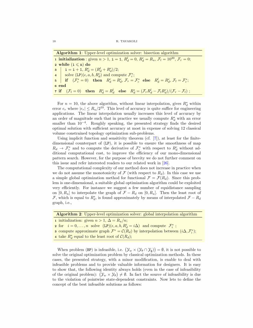
18 R. TAVAKOLI
Algorithm 1: Upper-level optimization solver: bisection algorithm
initialization : given n > 1, i = 1, Rld = 0, Rrd = Ru, Fl = 1020, Fr = 0;1
while (i 6 n) do2
i = i + 1, Rcd = (Rld +Rrd)/2;3
solve (LP)(ε, a, b, Rcd) and compute F∗c ;4
if (F∗c = 0) then Rrd = Rcd, Fr = F∗c else Rld = Rcd, Fl = F∗c ;5
end6
if (Fl = 0) then R∗d = Rld else R∗d = (FrRld −FlRrd)/(Fr −Fl) ;7
For n = 10, the above algorithm, without linear interpolation, gives R∗d withinerror er where |er| ≤ Ru/210. This level of accuracy is quite suffice for engineeringapplications. The linear interpolation usually increases this level of accuracy byan order of magnitude such that in practice we usually compute R∗d with an errorsmaller than 10−4. Roughly speaking, the presented strategy finds the desiredoptimal solution with sufficient accuracy at most in expense of solving 12 classicalvolume constrained topology optimization sub-problems.
Using implicit function and sensitivity theorem (cf. [7]), at least for the finite-dimensional counterpart of (LP), it is possible to ensure the smoothness of mapRd → F∗c and to compute the derivative of F∗c with respect to Rcd without ad-ditional computational cost, to improve the efficiency of our mono-dimensionalpattern search. However, for the purpose of brevity we do not further comment onthis issue and refer interested readers to our related work in [26].
The computational complexity of our method does not increase in practice whenwe do not assume the monotonicity of F (with respect to Rd). In this case we usea simple global optimization method for functional F = F(Rd). Since this prob-lem is one-dimensional, a suitable global optimization algorithm could be exploitedvery efficiently. For instance we suggest a few number of equidistance samplingon [0, Ru] to interpolate the graph of F − Rd on [0, Ru]. Then the least root ofF , which is equal to R∗d, is found approximately by means of interpolated F − Rdgraph, i.e.,
Algorithm 2: Upper-level optimization solver: global interpolation algorithm
initialization: given n > 1, ∆ = Ru/n;1
for i = 0, . . . , n solve (LP)(ε, a, b, Rid = i∆) and compute F∗i ;2
compute approximate graph F∗ = C(Rd) by interpolation between (i∆,F∗i );3
take R∗d equal to the least root of C(Rd);4
When problem (BP) is infeasible, i.e.(Yw × (Yθ ∩ Yg)
)= ∅, it is not possible to
solve the original optimization problem by classical optimization methods. In thesecases, the presented strategy, with a minor modification, is enable to deal withinfeasible problems and to provide valuable information for designers. It is easyto show that, the following identity always holds (even in the case of infeasibilityof the original problem):
(Yw × Yθ
)6= ∅. In fact the source of infeasibility is due
to the violation of pointwise state-dependent constraints. Now lets to define theconcept of the best infeasible solutions as follows:
AUTOMATIC OPTIMAL RISER DESIGN 19
Definition 7.3. Assume that for problem (BP) we have(Yw× (Yθ ∩Yg)
)= ∅, then
(w∗, θ∗) ∈(Yw × Yθ
)is called a best α-infeasible solution to (BP) if the following
condition holds:
Mα(w∗, θ∗) 6Mα(w, θ) ∀(w, θ) ∈(Yw × Yθ
),
where α ∈ [0, 1] is a user-defined (trade-off) parameter and the merit functionMα(·, ·) is defined as follows:
Mα := αRd + (1− α) F∗
where F∗ denotes the value of the objective functional at the local solution of thesub-problem (LP) for Rd = Rd.
In fact in the case of the problem infeasibility, we will have a bi-objective op-timization problem in which there is a trade-off between the consumed materialsresource weighted by factor α and the infeasibility of the state-dependent pointwiseconstraints weighted by factor (1−α). It is no need to emphasis that such solutionsare of value from the practical point of view.
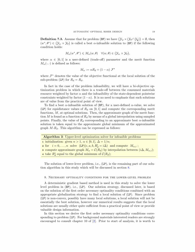
To find a best α-infeasible solution of (BP), for a user-defined α-value, we solve(LP) for equidistance values of Rd on [0, 1] and compute the corresponding meritfunctions, M , at optimal solutions. Then, the approximate graph of the merit func-tion M is found as a function of Rd by means of a global interpolation using sampledpoints. Finally, the value of Rd corresponding to an approximate best α-infeasiblesolution is taken equal to the approximate global minimum of the approximatedgraph M -Rd. This algorithm can be expressed as follows:
Algorithm 3: Upper-level optimization solver for infeasible problems
initialization: given n > 1, α ∈ [0, 1], ∆ = 1/n;1
for i = 0, . . . , n solve (LP)(ε, a, b, Rid = i∆) and compute Mα,i ;2
compute approximate graph Mα = C(Rd) by interpolation between (i∆,Mα,i);3
take R∗d equal to the global minimum of C(Rd);4
The solution of lower-lever problem, i.e., (LP), is the remaining part of our solu-tion algorithm in this study which will be discussed in section 8.
8. Necessary optimality conditions for the lower-level problem
A deterministic gradient based method is used in this study to solve the lowerlevel problem in (BP), i.e., (LP). Our solution strategy, discussed later, is basedon the solution of the first order necessary optimality conditions combined with anappropriate globalization strategy to find a local solution of (LP). Since problem(LP) is non-convex, possibly have many local solutions, a local solution will not beessentially the best solution, however our numerical results suggests that the localsolutions are usually either quite sufficient from a practical point of view or providevaluable design information.
In this section we derive the first order necessary optimality conditions corre-sponding to problem (LP). For background materials interested readers are stronglyencouraged to consult chapter 10 of [2]. Prior to start of analysis, it is worth to
20 R. TAVAKOLI
define the meaning of differentiability on function spaces. Note that there exist sev-eral differentiability notions in mathematical programming literature. The notionof Gateaux derivative is adapted in this study.
Definition 8.1. (Gateaux derivative, cf. [2]) Consider Banach spaces Y and Wand U as open subset of Y . A function f : U → W is called to be Gateauxdifferentiable at u ∈ U if for every test function v ∈ Y the following limit exist:
f ′(u) := limζ→0
f(u+ ζv)− f(u)
ζ
In this case we show the Gateaux derivative symbolically by f ′(u). If Y is a Hilbertspace, which is usually the case, then f ′(u) lives on the dual space of Y . Thereforeusing the Riesz representation theorem, there is a unique p ∈ Y such that 〈p, v〉 =f ′(u), where 〈·, ·〉 denotes the inner product on Y . In this case, without confusion,it is common to call p as the Gateaux derivative. We use notation df(u) in thiscase, i.e., df(u) = p. It is easy to verify that under some mild conditions (whichusually hold in practice) most of properties for classical derivatives have equivalentextension to Gateaux derivative. In the case of multi-variable functional, the partialGateaux derivative are denoted by f ′(·), ∂(·)f(· · · ) symbols in this study. For the
purpose of convenience the Gateaux derivative is called as the directional derivativein this study, henceforth.
Note. Since our goal in this study is not to do a rigorous mathematical analysis,we simply assume that our functions possess the regularities of suitable Hilbertspaces and continue our analysis on inner product spaces henceforth. We use thenotation 〈·, ·〉A :=
∫A(·)(·) dΩ to denote either of inner product or duality pairing
on the corresponding function spaces.Consider an arbitrary function η ∈ Xη(D), where Xη is a sufficiently regular
Banach space (it is identical to Xθ in practice). Lets to introduce the followingaugmented lagrangian by adding the inner product of η and the heat equation tothe objective functional corresponding to problem (LP):
L(w, θ, η) := F(θ) +
∫Q
η(ρc ∂tθ−∇ · (k∇θ)
)dQ+
∫Σ
η(k∇θ ·n−h∞(θ∞− θ)
)dΞ
where dΞ := dΓdt and dΓ denotes the surface measure induced on ∂D. The setof points satisfy the first order necessary optimality conditions for problem (LP),denoted by U can be expressed as follows (cf. [2]):
U :=
(w, θ, η) ∈(A×Xθ(D)×Xη(D)
) ∣∣∣∣∣ ∂wL(w, θ, η) = 0 in D (C.1)∂θL(w, θ, η) = 0 in D (C.2)∂ηL(w, θ, η) = 0 in D (C.3)
.
where ∂wL, ∂θL and ∂ηL denote respectively the partial directional derivatives ofL with respect to w, θ and η along arbitrary directions δw ∈ Xw(D), δθ ∈ Xθ(D)and δη ∈ Xη(D) respectively. In fact set U includes constrained stationary pointsof lagrangian L. Now, lets to define the following inner product notations, to keepour derivations concise:⟨
·, ·⟩Q
:=
∫T
⟨·, ·⟩D dt,
⟨·, ·⟩
Σ:=
∫T
⟨·, ·⟩∂D dt⟨
·, ·⟩Q0
:=⟨·, ·⟩D∣∣t=0
,⟨·, ·⟩QT
:=⟨·, ·⟩D∣∣t=T
AUTOMATIC OPTIMAL RISER DESIGN 21
For ∂wL in optimality condition (C.1) we have,⟨∂wL, δw
⟩D =
⟨η(∂wρc+ ρ∂w c) ∂tθ − η∇ · (∂wk∇θ), δw
⟩Q
+⟨η ∂wk∇θ · n, δw
⟩Σ
=⟨η(∂wρc+ ρ∂w c) ∂tθ + ∂wk∇η · ∇θ, δw
⟩Q
(8.1)
where,
∂wρ = pwp−1(ρc − ρm) (8.2)
∂w c = pwp−1(ce − cm) (8.3)
∂wk = pwp−1kckm(kc − km)(wp(km − kc) + kc
)−2(8.4)
Note that the boundary term in (8.1) is removed using integration by part followedby an application of the divergence theorem on the diffusion term.
For ∂θL within the optimality condition (C.2) we have,⟨∂θL, δθ
⟩D =
⟨dθF , δθ
⟩D +
⟨ηρ ∂θ c ∂tθ, δθ
⟩Q
+
∫Q
ηρc ∂t(δθ) dQ
−∫Q
η ∇ ·(k∇(δθ)
)dQ+
∫Σ
η k∇(δθ) · n dΞ +⟨h∞η, δθ
⟩Σ
:= I1 + I2 + I3 + I4 + I5 + I6 (8.5)
where,
∂θ c = wp ∂θ ce = wL(θl − θs)−1(dθHε(θ − θs)− dθHε(θ − θl)
)(8.6)
where the derivative of the regularized heaviside function with respect to its inputargument can be straightforwardly computed as follows,
dxHε(x) =
1/2ε
(1 + cos(πx/ε)
), −ε 6 x 6 ε
0, otherwise(8.7)
The integration by part simplifies I3 to:
I3 =⟨ρc η, ∂wθ
⟩QT−⟨ρc η, ∂wθ
⟩Q0−⟨ρc ∂tη, ∂wθ
⟩Q
:= I7 + I8 + I9 (8.8)
Since the initial conditions are independent from the temperature, I8 is equal tozero. Using the integration by part and divergence theorem to I4 results,
I4 =
∫Q
−∇ ·(kη ∇(δθ)
)dQ+
∫Q
k∇η · ∇(δθ) dQ
=
∫Σ
−kη∇(δθ) · n dΞ +
∫Q
∇ ·(δθ k ∇η
)dQ−
⟨∇ · (k ∇η), δθ
⟩Q
=
∫Σ
−kη∇(δθ) · n dΞ +⟨k∇η · n, δθ
⟩Σ−⟨∇ · (k ∇η), δθ
⟩Q
Therefore,
I4 + I5 =⟨k∇η · n, δθ
⟩Σ−⟨∇ · (k ∇η), δθ
⟩Q
:= I10 + I11 (8.9)
To compute term I1 in (8.5), lets to recall the structure of integrand, G, in thedefinition of functional F ,
G =
(min
(((∂tθ)
− 12 |∇θ| − gc
)δDa(atθ + bt
), 0))2
Ic
22 R. TAVAKOLI
In fact G is an explicit function of θ, ∂tθ and ∇θ. Therefore, for I1 we have,
I1 =⟨∂θF , δθ
⟩D +
⟨∂∇θF ,∇(δθ)
⟩D +
⟨∂∂tF , ∂t(δθ)
⟩D := J1 + J2 + J3 (8.10)
Lets to recall the following notations from previous sections,
g := (∂tθ)− 1
2 |∇θ| − gc), ge := g δDa (atθ + bt)
To avoid lengthy expressions, lets to define the following notations:
g := min(ge, 0), d := δDa(atθ + bt
), j :=
∂G∂(∂tθ)
= −(∂tθ)− 3
2 |∇θ| d g Ic
Although function min(x, 0) is not differentiable at x = 0, square of this functionis smooth and differentiable everywhere. For J1 in (8.10) we have,
J1 =⟨− a−2at (atθ + bt) g ge Ic, δθ
⟩D (8.11)
For J2 in (8.10) we have,
J2 =
∫Q
d g Ic|∇θ|√∂tθ∇θ · ∇(δθ) dQ
=⟨ d g Ic|∇θ|√∂tθ∇θ · n, δθ
⟩Σ−⟨∇ ·( d g Ic∇θ|∇θ|√∂tθ
), δθ
⟩D
:= J4 + J5 (8.12)
The boundary integral J4 in (8.12) is equal to zero, because the value of the indicator
function Ic on ∂D is equal to zero. Applying the integration by part on J3 in (8.10)results,
J3 =⟨j, δθ
⟩QT−⟨j, δθ
⟩Q0
−⟨dtj, δθ
⟩Q
:= J6 + J7 + J8 (8.13)
and,
dtj(θ, ∂tθ,∇θ) ≈ ∂θ j ∂tθ + ∂(∂tθ)j ∂ttθ + ∂(∇θ)j · ∇(∂tθ) (8.14)
where ∂tt(·) := ∂2(·)/∂t2 and j denotes the regularized form of function j in whichthe minimum function is replaced by the regularized minimum function to ensurethe differentiability. Considering the identity min(x, 0) = x(1−H(x)), the regular-
ized minimum function in this study, denoted by min, is defined as follow,
min(x, 0) := x(1− Hε(x)) (8.15)
The regularization parameter ε corresponding to (8.15) is taken equal to one spatialgrid-size in this study. Because of the uniform initial temperature distributionwithin the casting, ignoring smoothing effects of Ic on the cast-mold boundaries,we take Ic∇θ(t = 0,x) ≈ 0 which results J7 ≈ 0. Using the regularized minimumfunction in the objective functional makes it as a direct function of w, however thisdependency is very weak and is ignored in this study. Since the expansion of termsin (8.14) is a straightforward job, we leave further simplification of (8.14) to savethe space.
The optimality condition (C.3), i.e., ∂ηL = 0 in D is equivalent to the heatequation in problem (LP), therefore (C.3) holds when θ solves the heat equation in(LP).
AUTOMATIC OPTIMAL RISER DESIGN 23
To enforce the condition (C.2), we collect the inner products terms include δθand introducing the following adjoint heat equation:
(AH)(θ) :=
−ρ(w)c(w) ∂tη = ∇ · (k(w)∇η)− ηSa(x) + Sb(x) in Q−k(w)∇η · n = h∞η on Σ
η(t,x) = η0(x) in Q0
where,
Sa(x) = wpρ(w)L(θl − θs)−1(dθHε(θ − θs)− dθHε(θ − θl)
)∂tθ (8.16)
Sb(x) = a−2at(atθ + bt)gge Ic +∇ ·(dg
∇θ|∇θ|√∂tθIc)
+ dtj (8.17)
η0(x) =(ρ(w)c(w)
)−1(∂tθ)
− 32 |∇θ|dgIc (8.18)
In derivation of problem (AH), the differential operators are resulted from the collec-tion of I9, I11, the first source term is due to I2, the second source term is formedby collection of J1, J5, J8, the initial conditions are resulted from I7, J6 and theboundary conditions are due to the collection of I6, I10. Note that the adjointheat equation (AH) should be integrated in reverse time direction, i.e., from t = Tto t = 0 (consider the negative sign of transient term in the corresponding PDE).It is clear that the solution of direct heat equation should be a-priori available tosolve problem (AH). The direct heat equation, denoted by (DH), can be expressedas follows,
(DH) :=
ρ(w)c(w) ∂tθ = ∇ · (k(w)∇θ) in Qk(w)∇θ · n = h∞(θ∞ − θ) on Σ
θ(t,x) = θ0(x) in Q0
where θ0(x) := wpθp + (1− wp)θ∞.Now lets to state the optimality conditions based on the projected gradient to
develop our solution algorithm. For this purpose we first recall some known results.
Theorem 8.2. (orthogonal projection over a convex set, theorem 12.1.10 of [2])Let V be a Hilbert space and K as a convex closed nonempty subset of V . For allu ∈ V , there exists a unique uK ∈ K such that
‖u− uK‖22 = arg minv∈K‖u− v‖22.
The orthogonal projection of u onto set K is shown by operator PK(u)henceforth in this paper, i.e., uK = PK(u). Equivalently, uK is characterizedby the following property:
uK ∈ K, 〈uK − u, v − uK〉 > 0, ∀v ∈ K (8.19)
Theorem 8.3. (Euler inequality for convex sets, theorem 10.2.1 of [2]) Let V be aHilbert space and K as a convex closed nonempty subset of V . Assume functionalJ(u) : K → R is differentiable at u ∈ K with the directional derivative denoted byJ ′(u). If u be a local minimum point of J(u) over K then:
〈J ′(u), v − u〉 > 0, ∀v ∈ K (8.20)
Corollary 8.4. (necessary optimality conditions based on the projected gradient)Let V be a Hilbert space and K as a convex closed nonempty subset of V . Assume
24 R. TAVAKOLI
functional J(u) : K → R is differentiable at u ∈ K with the directional derivativedenoted by J ′(u). If u be a local minimum point of J(u) over K then:
J ′K,µ(u) = 0 almost everywhere, J ′K,µ(u) = PK(u− µJ ′)− u (8.21)
where µ ∈ R+. Since PK(u−µJ ′)−u is equivalent to the scaled projected gradient,constrained stationary points of J are zeros of the scaled projected gradient withrespect to set K. Therefore we call (8.21) as the necessary optimality conditionsbased on the projected gradient.
Proof. Considering an arbitrary µ ∈ R+, by (8.20) we have:
〈µJ ′(u), v − u〉 > 0, ∀v ∈ KSimple algebra results:⟨
u−(u− µJ ′(u)
), v − u
⟩> 0, ∀v ∈ K (8.22)
Comparing (8.19) and (8.22) results
u = PK(u− µJ ′(u)
)almost everywhere which complete the proof.
Corollary 8.5. (descent property of the scaled projected gradient) Let V be a Hilbertspace and K as a convex closed nonempty subset of V . Assume functional J(u) :K → R is differentiable at u ∈ K with the directional derivative denoted by J ′(u).Assume that the scaled projected gradient at u ∈ K is denoted by J ′K,µ(u), i.e.,
J ′K,µ(u) = PK(u− µJ ′)− u. Then for all u ∈ K and µ ∈ R+ we have:
〈J ′(u), J ′K,µ(u)〉 6 − 1
2µ‖J ′K,µ(u)‖22 (8.23)
Proof. According to the definition of the projection operator we have:
PK(u− µJ ′(u)) = arg minv∈K‖v − (u− µJ ′(u))‖22
since u, v ∈ K we have,
‖v − (u− µJ ′(u))‖22 6 ‖µJ ′(u)‖22the expansion of left hand side results,
2µ⟨J ′(u), v − u
⟩6 −‖v − u‖22
since v is an arbitrary member of K we replace it by PK(u−µJ ′(u)) which results,
2µ⟨J ′(u), PK(u− µJ ′(u))− u
⟩6 −‖PK(u− µJ ′(u))− u‖22
and backing to the definition of J ′K,µ complete the proof.
Corollary 8.5 suggests a simple iterative gradient descent method to find localminimums of convex constrained optimization problems. Assuming iteration levelis denoted by m and considering initial guess u0, we have:
um+1 = um + νmJ′K,µm(um), m = 0, 1, . . . , (8.24)
where νm ∈ (0, 1]. In the present study the scaling parameter µm is selected basedon the Barzilai-Borwein (BB) step-size [3]:
µm = 〈sm−1, sm−1〉/〈sm−1, rm−1〉,
AUTOMATIC OPTIMAL RISER DESIGN 25
where sm := um − um−1 and rm := J ′(um) − J ′(um−1). The main benefit ofusing BB step-size is its spectral properties which makes it as a cheap and veryefficient method to approximately solve large-scale problems (cf. [8]). To ensurethe global convergence, it is required that νm is selected based on a globalizationstrategy like a line-search algorithm. However, it is clear that using a monotonicline-search algorithm reduces (8.24) iterations to classical projected steepest descentmethod, i.e., we miss promising properties of BB step-size. To cope this problem,the nonmonotone globalization strategy suggested in [8] is used in this study. Formore details refer to: [8].
Combining the above results we can state the first order necessary optimalityconditions for problem (LP), denoted by (OC) as follows:
(OC) :=
ρ(w)c(w) ∂tθ = ∇ · (k(w)∇θ) in Qk(w)∇θ · n = h∞(θ∞ − θ) on Σ
θ(t,x) = θ0(x) in Q0
−ρ(w)c(w) ∂tη = ∇ · (k(w)∇η)− ηSa(x) + Sb(x) in Q−k(w)∇η · n = h∞η on Σ
η(t,x) = η0(x) in Q0
PA(w − ∂wL)− w = 0 in DTo keep the coherency of arguments in this study, lets to briefly outline the
optimization algorithm used to solve problem (LP). To avoid technical difficul-ties, we sate our algorithm for discretized version of our original problem (detailsof discretization method will be discussed later). Lets to denote by (LP)h, (OC)h,(DH)h and (AH)h, the finite dimensional counterpart problems corresponding to (LP),(OC), (DH) and (AH) respectively which are resulted after the temporal-spatial dis-cretization of (LP). Assume θ and η solve problems (DH)h, (AH)h respectively, theoptimal value of w is found using the nonmonotone globalized version of iteration(8.24). This algorithm is in fact identical to nonmonotone spectral projected gradi-ent (SPG) method introduced in [8]. More precisely, the SPG2 algorithm presentedin [8, 9] is used in this study. To use SPG2 in this regard, it is suffice to remarkthat whenever SGP2 asks for the objective functional value, (DH)h should be solvedusing current value of w-filed and then the objective function should be evaluated.Similarly, when SGP2 asks for the gradient of the objective functional, it is requiredto solve (DH)h and (AH)h respectively and, then to compute ∂wL using (8.1). Theinput parameters for SPG2 algorithm in this study are identical to set of defaultparameters in [9].
As discussed in [8], the efficiency of SPG2 mainly relay on the existence of anefficient way to project trial steps onto the feasible set of solutions (is a user-definedfunction in SPG2 algorithm), i.e., PA(·) operator in the present study. Therefore,introducing an efficient method for the projection onto the admissible domain ofcontrol parameters is the remaining part of our optimization algorithm in this studywhich is discussed in section 9.
9. Projection onto the admissible control domain
Assume that the admissible control domain of w is nonempty, i.e., A 6= ∅. Sinceall constraints define A are linear functions of w, A is a closed convex subset of
26 R. TAVAKOLI
L2(D). Consider an arbitrary control variable w with at least an L2(D) regularity.According to theorem 8.2, there is a unique wA ∈ A where:
wA = PA(w) := arg minw∈A
1
2‖wA − w‖2. (9.1)
Lets to redefine the projection problem (9.1) as follows:
arg minw∈Bw
1
2‖wA − w‖2 s.t. :
∫Ddw(x) dΩ = bd,
∫Ddn
w(x) dΩ 6 bdn, (9.2)
where bd = VdRd, bdn = VdnRdn and,
Bw :=w ∈ Xw(D)
∣∣ wL 6 w 6 wU where inequalities in the definition of Bw are to be understood pointwise and,
wL :=
w ∈ Xw(D)
∣∣ wL(x) = 1 in QcwL(x) = 0 in Q \Qc
.
wU :=
w ∈ Xw(D)
∣∣ wU (x) = 1 in Qc ∪QdwU (x) = 0 in Qr \Qd
.
Note that the constraint w = 0 on Σ in A is applied independently as a boundarycondition in this study and so is not included here. Since the projection operatorhere is time independent, we can perform our analysis only on spatial part Q. It isevident that wA is alternatively equal to unique constrained (w ∈ Bw) stationarypoint of the following augmented lagrangian:
M(λd, λdn, w) :=1
2‖wA − w‖2 + λd
( ∫Ddw dΩ− bd
)+ λdn
( ∫Ddn
w dΩ− bdn)
where λd, λdn ∈ R are lagrange multipliers corresponding to the integral equalityand inequality constraints in (9.2) respectively. The constrained stationary pointof M is characterized by identity,
∂λdM(λd, λdn, w) = ∂λnM(λd, λdn, w) = ∂wM(λd, λdn, w) = 0, (9.3)
together with w ∈ Bw and the complementarity conditions,
λdn( ∫Ddn
w dΩ− bdn)
= 0, λdn > 0
for the qualification of the corresponding integral inequality constraint. The firstand second conditions in (9.3) are equivalent to satisfaction of the integral equalityand inequality constraints respectively. Consider an arbitrary test function δw ∈Xw(D), for the partial directional derivative of M with respect to δw we have,⟨
∂wM, δw⟩D =
⟨∂wwA − w, δw
⟩D +
∫Ddλdδw dΩ +
∫Ddn
λdnδw dΩ (9.4)
denoting by Id and Idn the characteristic functions corresponding to the spatialdomains Dd and Ddn, (9.4) can be written as follows:⟨
∂wM, δw⟩D =
⟨∂wwA − w, δw
⟩D +
∫DλdδwId dΩ +
∫DλdnδwIdn dΩ (9.5)
(9.5) simplifies to:⟨∂wM, δw
⟩D =
⟨∂wwA − w + λdId + λdnIdn, δw
⟩D (9.6)
AUTOMATIC OPTIMAL RISER DESIGN 27
Therefore, the following condition holds the third condition of (9.3) in an almosteverywhere sense within D:
wA − w + λdId + λdnIdn = 0, almost everywhere in D (9.7)
To enforce the bound constraints, w ∈ Bw, the necessary optimality conditionsbased on the projected gradient method, corollary 8.4, is used here. Therefore,the constrained stationary point of M should satisfy the following condition in analmost everywhere sense within D:
wA − PBw(w − λdId − λdnIdn
)= 0, almost everywhere in D (9.8)
Backing to the definition of domains Dd and Ddn in section 2 we have Idn ⊆ Id.Therefore, we can decompose (9.8) into the following independent conditions definedin non-overlapping parts of D:
wA − PBw(w)
= 0, almost everywhere in D \ Dd,wA − PBw
(w − λd
)= 0, almost everywhere in Dd \ Ddn,
wA − PBw(w − λd − λdn
)= 0, almost everywhere in Ddn
It is well-know that the projection onto the bound constraints is separable and canbe explicitly computed as follows (cf. chapter 10 of [2]):
PBw(w) = mid(wL, w, wu),
where the median operator, mid(·, ·, ·), is to be understood pointwise here and isdefined as follows,
mid(a, b, c) := min(c, max(a, b)),
where a, b, c ∈ R and a 6 c. Therefore we have:
wA = mid(wL, w, wu), almost everywhere in D \ Dd, (9.9)
wA = mid(wL, w − λd, wu), almost everywhere in Dd \ Ddn, (9.10)
wA = mid(wL, w − λd − λdn, wu), almost everywhere in Ddn (9.11)
It is clear that (9.9) has an explicit evident solution. However, to solve (9.10)and (9.11), the values of λd and λdn at the optimal solution are required. Forthis purpose we use from our integral constraints and consider two different cases:(i) the integral inequality constraint is inactive at the optimal solution, (ii) theintegral inequality constraint is active at the optimal solution. Since lagrangianMis strictly convex, it admits only one stationary point. Therefore only one of theabove cases happens in practice.
If case (i) happens at the optimal solution, the complementarity condition enforcethat λdn = 0 and so λd is equal to the unique root of the following mono-variablenonlinear equation:
f1(λd) = bd −∫Dd
mid(wL, w − λd, wu) dΩ = 0 (9.12)
In the other case, the integral inequality constraint is active at the optimal solution,i.e., we have
∫Ddn wA dΩ = bdn. In this case, the optimal value of λd is equal to
the unique root of the following mono-variable nonlinear equation:
f2(λd) = bd − bdn −∫Dd\Ddn
mid(wL, w − λd, wu) dΩ = 0 (9.13)
28 R. TAVAKOLI
Having the optimal value of λd from (9.13), the optimal value of λdn is equal to theunique root of the following equation:
f3(λdn) = bdn −∫Ddn
mid(wL, w − λd − λdn, wu) dΩ = 0 (9.14)
Therefore the remaining job here is to suggest an efficient way to compute uniqueroots of functions f1, f2 and f3. The result of the following lemma is employed forthis purpose.
Lemma 9.1. Functions f1(λd), f2(λd) and f3(λdn) are continuous piecewise linearand monotonically non-increasing functions of their arguments.
Proof. We present the proof here only for function f1. The extension of proof forthe other cases is straightforward. Lets to define functions λLd and λUd , with at leastan L2(Dd) regularity, as follows:
λLd = w − wL, λUd = w − wU ,where the above relations are to be understood pointwise. It is clear that λUd 6 λ
Ld .
Note that wL = 0 and wU = 1 in Dd. Considering (9.10) and (9.11) we have (recallthat in this case λdn = 0):
wA(λd) =
wU , if λ 6 λUd ,w − λd, if λUd 6 λ 6 λ
Ld ,
wL, if λ > λLd .(9.15)
where all algebra in (9.15) are to be understood pointwise. Considering (9.15),wA(λd) is a continuous piecewise linear and monotonically non-increasing functionof λd. Since we have f1(λd) = bd−
∫Dd wA dΩ, f1(λd) is also a continuous piecewise
linear and monotonically non-increasing function of λd.
Using lemma 9.1 we can find unique roots of f1, f2 and f3 efficiently using thebisection method. The following corollary provides valuable information to selectthe initial search interval for the bisection method. We state the corollary only forfunction f1, but, the same results can be easily obtained for f2 and f3 which areignored here to save the space.
Corollary 9.2. Consider functions λLd and λUd as defined in lemma 9.1. Let ϑ ∈ Rsuch that ϑ = max ‖λLd ‖∞ , ‖λUd ‖∞ , then f1(−ϑ)f1(ϑ) 6 0, i.e., the root of f1
happens within interval [−ϑ, ϑ ]. Moreover f1(λd) 6 0 for λd 6 −ϑ and f1(λd) > 0for λd > −ϑ.
Proof. Since f1(λd) is a continuous piecewise linear and monotonically non-increasingfunction of λd and it has a unique root, we should have f1(λd) 6 0 for λd 6 −ϑand f1(λd) > 0 for λd > −ϑ. Therefore, the root happens in [−ϑ, ϑ ].
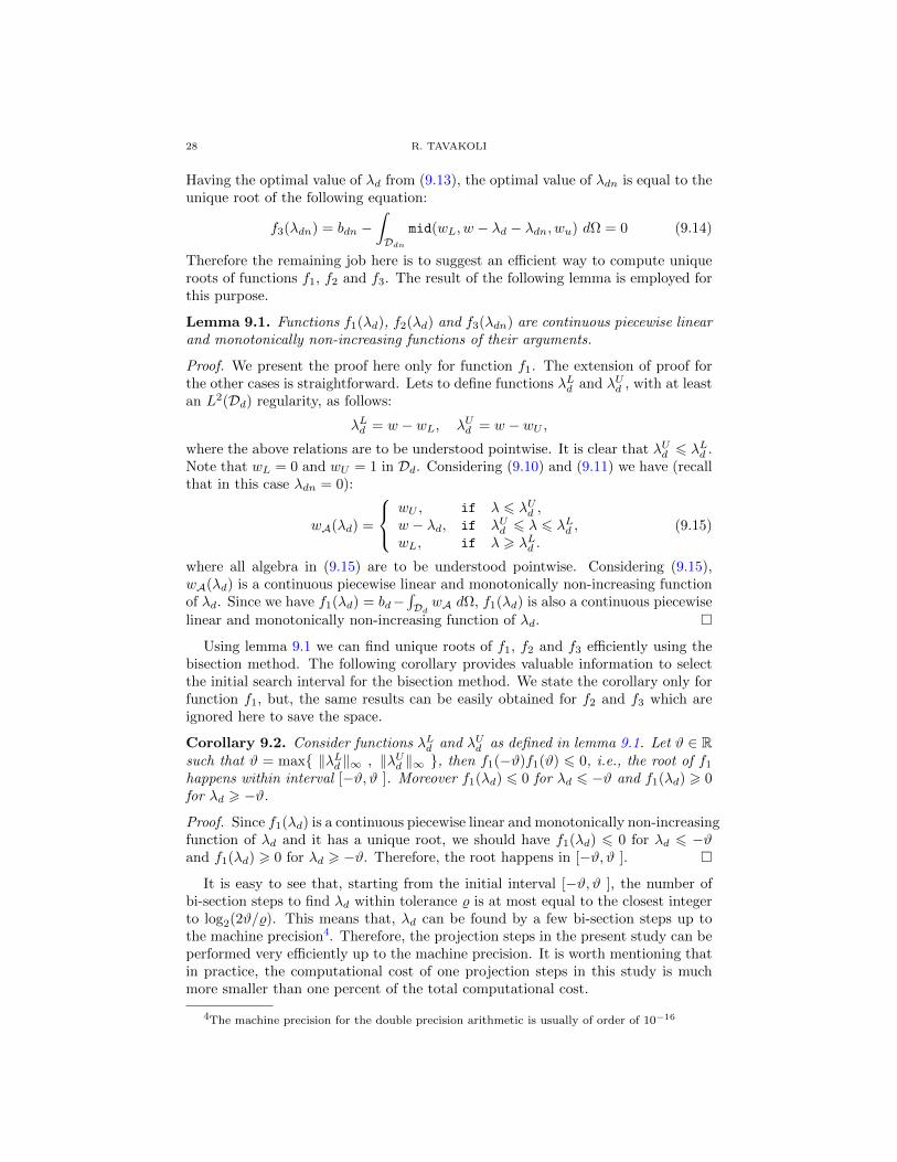
It is easy to see that, starting from the initial interval [−ϑ, ϑ ], the number ofbi-section steps to find λd within tolerance % is at most equal to the closest integerto log2(2ϑ/%). This means that, λd can be found by a few bi-section steps up tothe machine precision4. Therefore, the projection steps in the present study can beperformed very efficiently up to the machine precision. It is worth mentioning thatin practice, the computational cost of one projection steps in this study is muchmore smaller than one percent of the total computational cost.
4The machine precision for the double precision arithmetic is usually of order of 10−16
AUTOMATIC OPTIMAL RISER DESIGN 29
10. Numerical method
For the purpose of the numerical solution, the spatial domain D is decomposedinto a uniform Cartesian grid with the grid spacing ∆x; a user-defined parame-ter. The Cartesian grid generator CartGen [24] is used in this study to discretizecomplex geometries. Although a Cartesian grid makes an stair-case approxima-tion to curved boundaries, our numerical experiments showed that such grids arequite sufficient for the purpose of the solidification analysis, for instance see: [27].The temporal domain is also decomposed into a uniform grid with grid spacing ∆twhich is determined based on the stability criteria related to fully explicit solutionof the heat equation. Except for terms ∂tθ and ∂tη in the heat equations, all dif-ferential operators are discretized by means of cell-centered finite volume methodusing second order central schemes. Since the temporal concentration of pointwisestate-dependent constraints are sufficiently far from t = 0 and t = T in practice, wedo not need one-sided difference methods to evaluate dtj in the source term of theadjoint heat equation. The heat equations are integrated along the time axis usingthe first order fully explicit method. It poses an upper bound on ∆t. Because ourPDEs are highly nonlinear and include spatio-temporal concentrated source terms,using large time steps disturbs the accuracy of computations. The main reason forthe selection of fully explicit time integration method is due to the efficiency andability to capture details of solidification (and adjoint solidification) dynamics witha reasonable accuracy. The temporal integrations are computed using the classicaltrapezoidal integration method.
The main difficulty of using explicit time integration method is that the numberof time steps is very large in practice (commonly range from 103-104). This makesa difficulty during the computation of adjoint heat source and the objective func-tional derivative, because the whole temperature history should be stored prior tocomputation of these terms. This is a memory expensive procedure, dealing withlarge scale problems. For instance to store a double precision floating point θ-fieldwhich include 106 data for 104 time steps about 100 GB memory is needed.
A common way to manage this problem is the recursive windowingapproach presented in [4]. However this method is very expensive whenthe number of time steps is sufficiently large. In the present studya very simple but efficient method is used to cope this problem. Wesimply store θ-field on the hard-disk after each time step and read itfrom the disk whenever it is required. According to our experience theCPU cost of a read and write operation for one θ-field is smaller than thecost of one forward-backward time-step. Therefore, the computationalcost of our algorithm will be doubled in the worst conditions. Note thatthe available storage on the hard-disk is usually sufficient to manage ourdesired problems.
The topological instability is one of the most common difficulty related to thenumerical solution of topology optimization problems (see [6] for more details).A common treatment for this problem is using minimum length-scale control orsmoothing methods. However, as already mentioned in section 5, our nu-merical solution in the present study is free from this problem.
30 R. TAVAKOLI
11. Numerical results
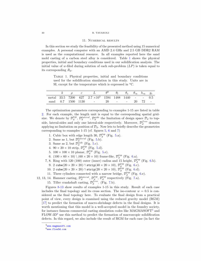
In this section we study the feasibility of the presented method using 15 numericalexamples. A personal computer with an AMD 2.4 GHz and 2.5 GB DDR2 RAMis used as the computational resource. In all examples reported here the sandmold casting of a carbon steel alloy is considered. Table 1 shows the physicalproperties, initial and boundary conditions used in our solidification analysis. Theinitial value of w-filed during solution of each sub-problem (LP ) is taken equal toits corresponding Rd.
Table 1. Physical properties, initial and boundary conditionsused for the solidification simulation in this study. Units are inSI, except for the temperature which is expressed in oC.
k ρ c L θ0 θl θs θ∞ h∞ gc
metal 33.5 7200 627 2.7 ×10⁵ 1594 1488 1440 - - 0.5sand 0.7 1500 1130 - 20 - - 20 72 -
The optimization parameters corresponding to examples 1-15 are listed in table2. For each example, the length unit is equal to the corresponding spatial grid-size. We denote by Dtopd , Dlaterald , Dsided the limitation of design space Dd to top-
side, lateral-sides and only one lateral-side respectively. Moreover, Dfreed denotesapplying no limitation on position of Dd. Now lets to briefly describe the geometriescorresponding to examples 1-15 (cf. figures 5, 6 and 7)
1. Cubic box with edge length 30, Dtopd (Fig. 5.a).
2. Same as 1, but Dlaterald (Fig. 5.b).3. Same as 2, but Dsided (Fig. 5.c).
4. 90× 20× 10 strip, Dtopd (Fig. 5.d).
5. 100× 100× 10 planar, Dtopd (Fig. 5.e).
6. (100× 60× 10) \ (60× 20× 10) frame-like, Dtopd (Fig. 6.a).
7, 8. Ring with 120 (100) outer (inner) radius and 15 height, Dtopd (Fig. 6.b).
9. 2 cube(20× 20× 20) ∩ strip(40× 20× 10), Dtopd (Fig. 6.c).
10. 2 cube(20× 20× 20) ∩ strip(20× 20× 10), Dtopd (Fig. 6.d).
11. Three cylinders connected with a narrow bridge, Dtopd (Fig. 6.e).
12, 13, 14. Hammer casting, Dlaterald , Dtopd , Dtopd respectively (Fig. 7.a).
15. Tiller crankshaft casting, Dfreed . (Fig. 7.b).
Figures 8-13 show results of examples 1-15 in this study. Result of each caseincludes the final topology and its cross section. The iso-contour w = 0.5 is con-sidered as the final topology here. To evaluate the final design from a practicalpoint of view, every design is examined using the reduced gravity model (RGM)[17] to predict the formation of macro-shrinkage defects in the final designs. It isworth mentioning that this model is a well-accepted model in the foundry society,for instance famous commercial casting simulation codes like MAGMASOFT5 andFLOW-3D6 use this method to predict the formation of macroscopic solidificationdefects. In this regard, we also include the result of RGM for each case (in fact the
5www.magmasoft.com6www.flow3d.com
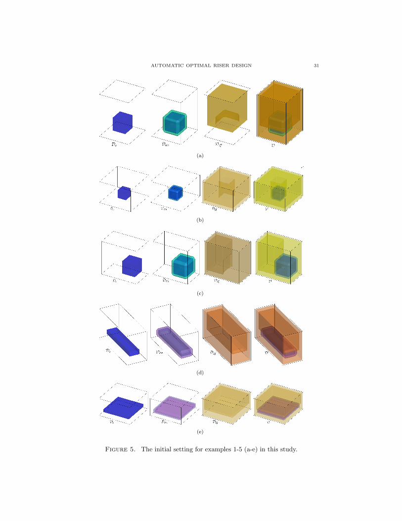
AUTOMATIC OPTIMAL RISER DESIGN 31
(a)
(b)
(c)
(d)
(e)
Figure 5. The initial setting for examples 1-5 (a-e) in this study.
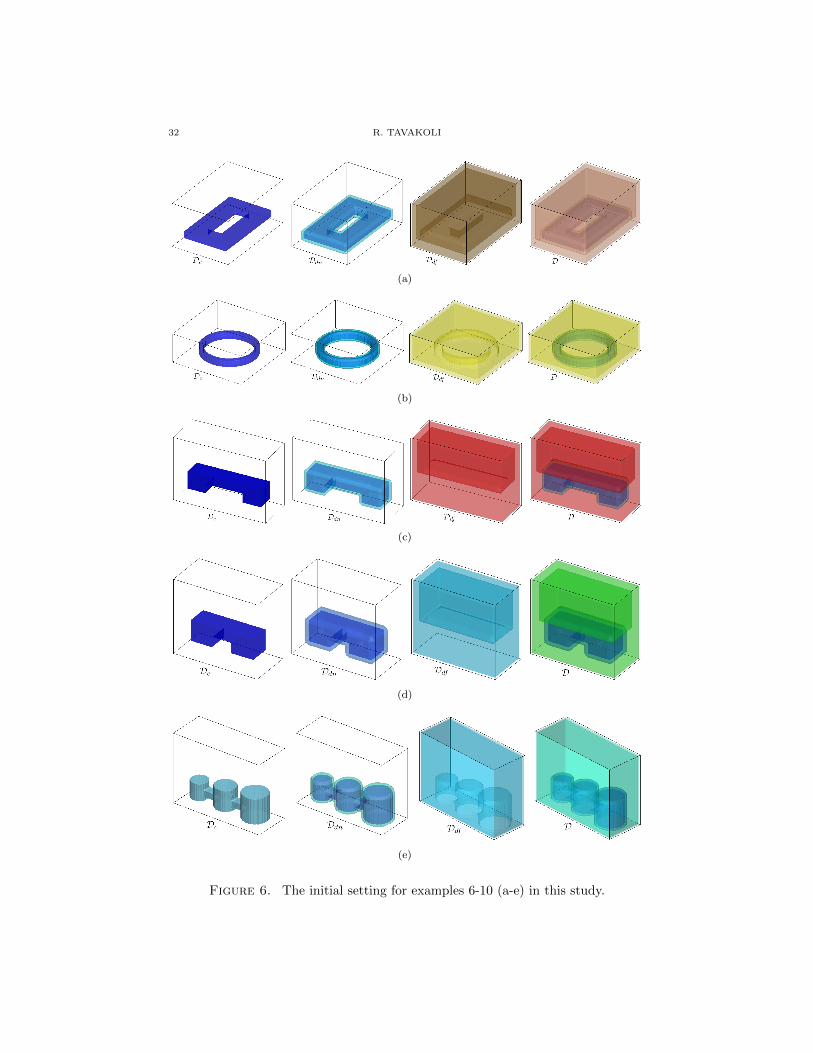
32 R. TAVAKOLI
(a)
(b)
(c)
(d)
(e)
Figure 6. The initial setting for examples 6-10 (a-e) in this study.
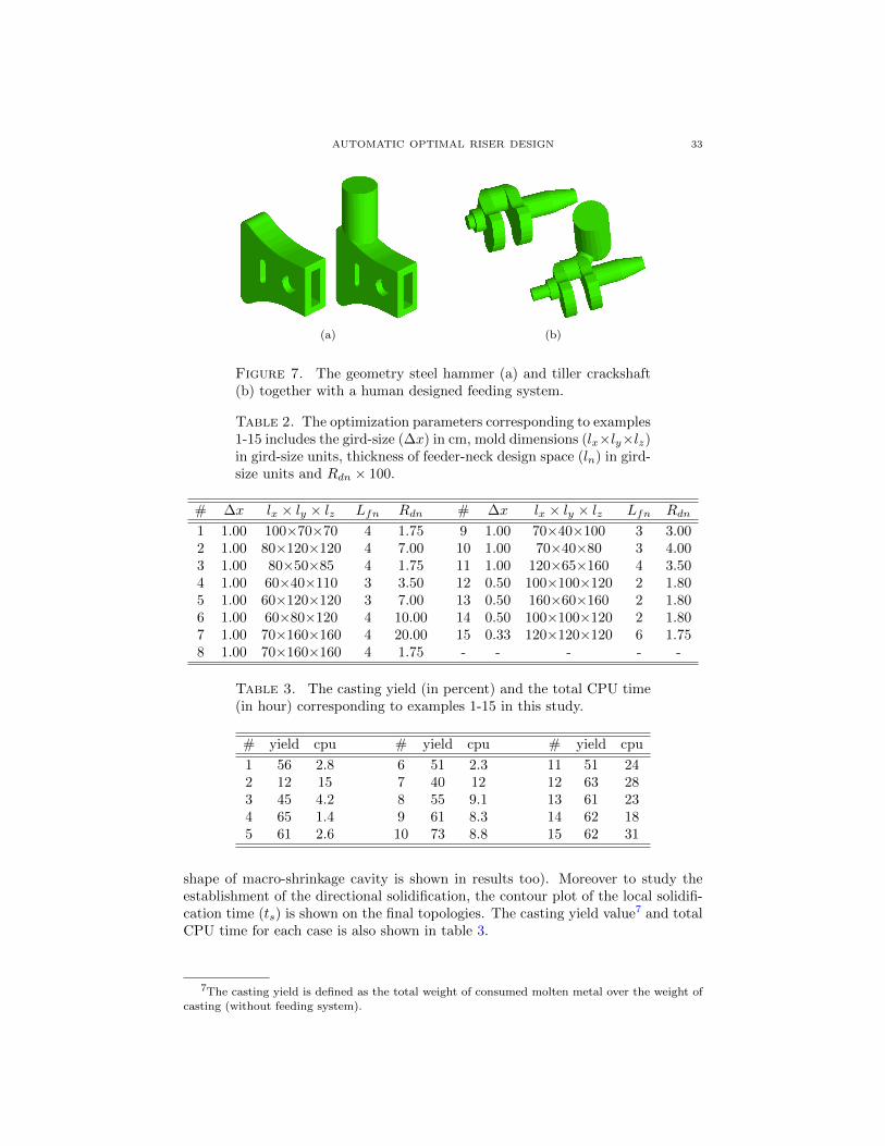
AUTOMATIC OPTIMAL RISER DESIGN 33
(a) (b)
Figure 7. The geometry steel hammer (a) and tiller crackshaft(b) together with a human designed feeding system.
Table 2. The optimization parameters corresponding to examples1-15 includes the gird-size (∆x) in cm, mold dimensions (lx×ly×lz)in gird-size units, thickness of feeder-neck design space (ln) in gird-size units and Rdn × 100.
# ∆x lx × ly × lz Lfn Rdn # ∆x lx × ly × lz Lfn Rdn
1 1.00 100×70×70 4 1.75 9 1.00 70×40×100 3 3.002 1.00 80×120×120 4 7.00 10 1.00 70×40×80 3 4.003 1.00 80×50×85 4 1.75 11 1.00 120×65×160 4 3.504 1.00 60×40×110 3 3.50 12 0.50 100×100×120 2 1.805 1.00 60×120×120 3 7.00 13 0.50 160×60×160 2 1.806 1.00 60×80×120 4 10.00 14 0.50 100×100×120 2 1.807 1.00 70×160×160 4 20.00 15 0.33 120×120×120 6 1.758 1.00 70×160×160 4 1.75 - - - - -
Table 3. The casting yield (in percent) and the total CPU time(in hour) corresponding to examples 1-15 in this study.
# yield cpu # yield cpu # yield cpu
1 56 2.8 6 51 2.3 11 51 242 12 15 7 40 12 12 63 283 45 4.2 8 55 9.1 13 61 234 65 1.4 9 61 8.3 14 62 185 61 2.6 10 73 8.8 15 62 31
shape of macro-shrinkage cavity is shown in results too). Moreover to study theestablishment of the directional solidification, the contour plot of the local solidifi-cation time (ts) is shown on the final topologies. The casting yield value7 and totalCPU time for each case is also shown in table 3.
7The casting yield is defined as the total weight of consumed molten metal over the weight ofcasting (without feeding system).
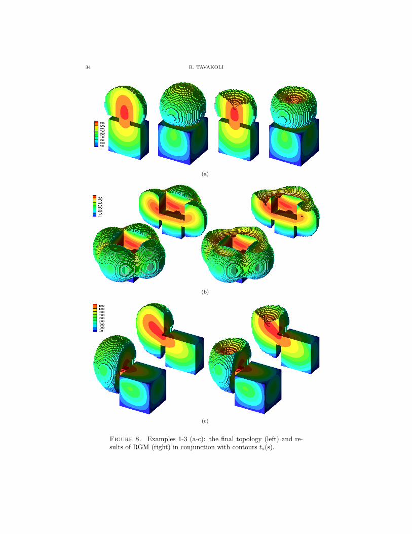
34 R. TAVAKOLI
(a)
(b)
(c)
Figure 8. Examples 1-3 (a-c): the final topology (left) and re-sults of RGM (right) in conjunction with contours ts(s).
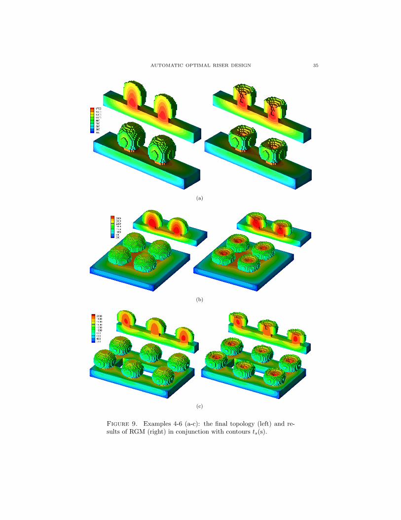
AUTOMATIC OPTIMAL RISER DESIGN 35
(a)
(b)
(c)
Figure 9. Examples 4-6 (a-c): the final topology (left) and re-sults of RGM (right) in conjunction with contours ts(s).
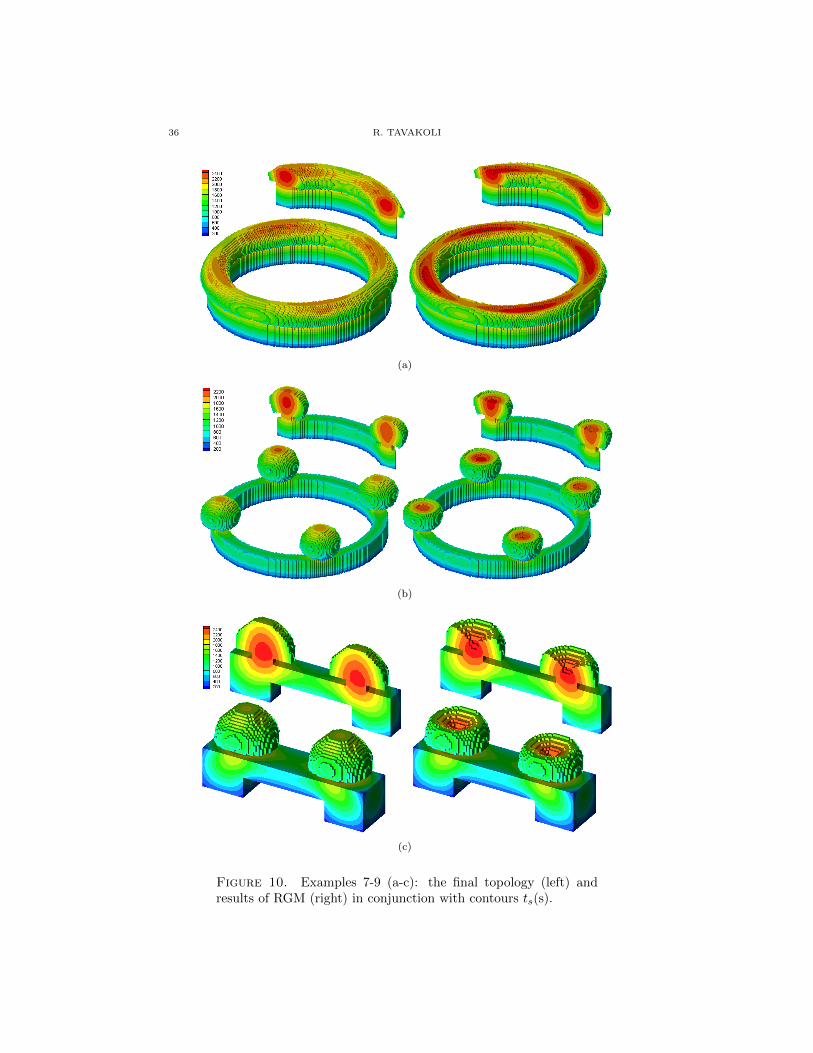
36 R. TAVAKOLI
(a)
(b)
(c)
Figure 10. Examples 7-9 (a-c): the final topology (left) andresults of RGM (right) in conjunction with contours ts(s).
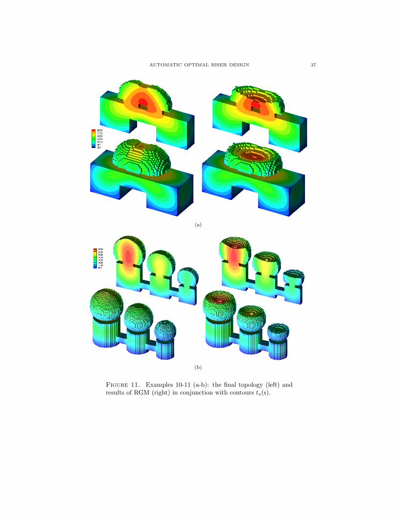
AUTOMATIC OPTIMAL RISER DESIGN 37
(a)
(b)
Figure 11. Examples 10-11 (a-b): the final topology (left) andresults of RGM (right) in conjunction with contours ts(s).
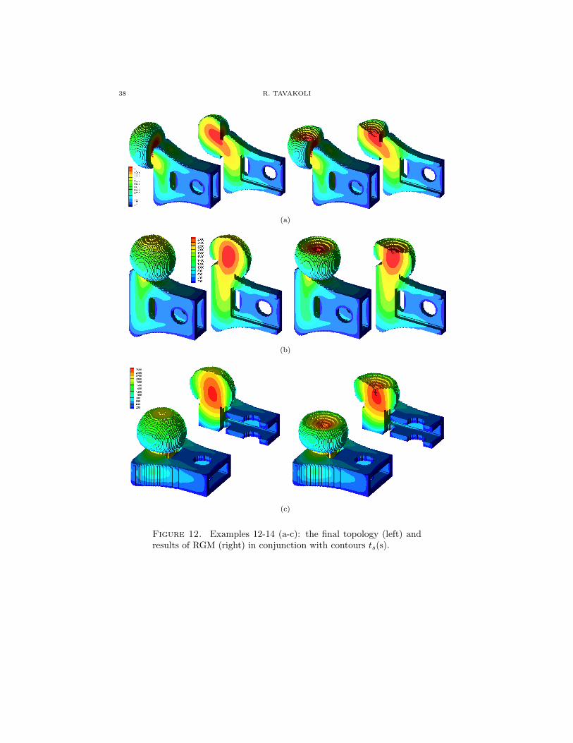
38 R. TAVAKOLI
(a)
(b)
(c)
Figure 12. Examples 12-14 (a-c): the final topology (left) andresults of RGM (right) in conjunction with contours ts(s).
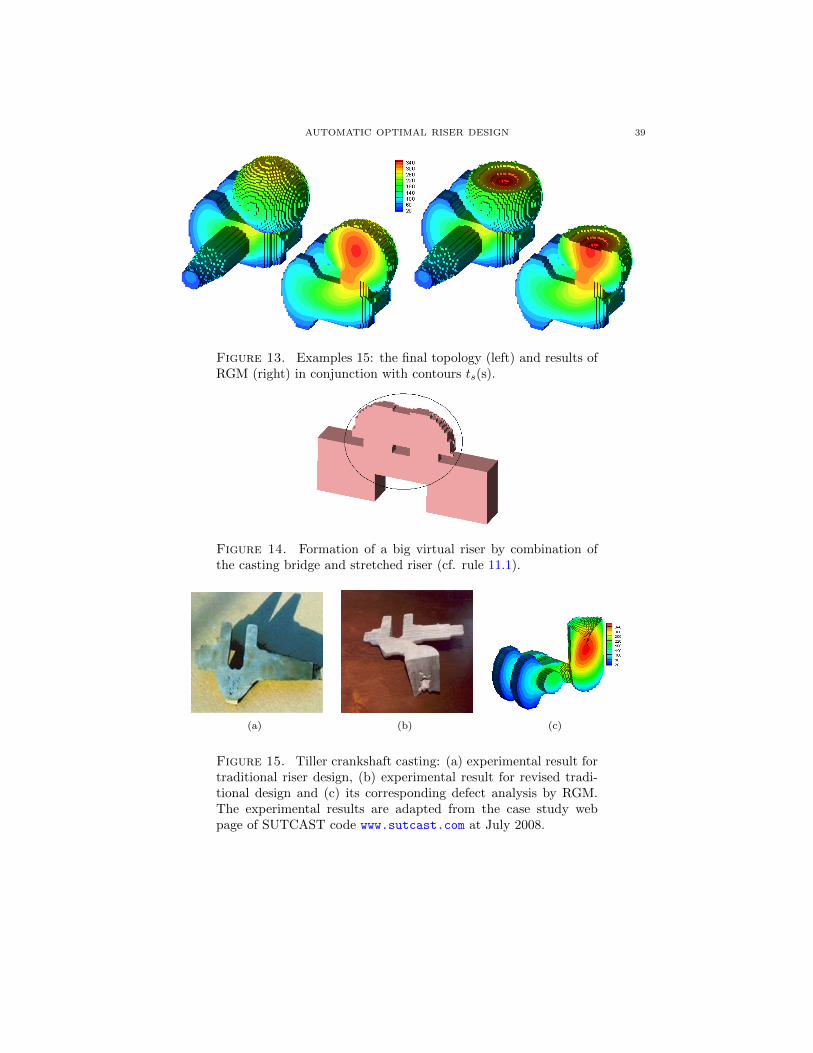
AUTOMATIC OPTIMAL RISER DESIGN 39
Figure 13. Examples 15: the final topology (left) and results ofRGM (right) in conjunction with contours ts(s).
Figure 14. Formation of a big virtual riser by combination ofthe casting bridge and stretched riser (cf. rule 11.1).
(a) (b) (c)
Figure 15. Tiller crankshaft casting: (a) experimental result fortraditional riser design, (b) experimental result for revised tradi-tional design and (c) its corresponding defect analysis by RGM.The experimental results are adapted from the case study webpage of SUTCAST code www.sutcast.com at July 2008.
40 R. TAVAKOLI
According to achieved results the directional solidification is well establishedin all cases and the final design is sound under both the Niyama criterion andthe RGM. The design of riser and riser-neck seems to be reasonable and manu-facturable; of course ignoring the molding constraints which is not considered inthis study. The reported CPU time in table 3 shows surprising efficiency of thepresented method, makes it a reasonable tool to solve large scale real-world prob-lems. Therefore, we can roughly conclude the success, validity and efficiency of thepresented mathematical model and its corresponding solution method.
The results also implies that the produced designs by our model are conservativeunder an evaluation by the RGM. We believe that this is due to this face thatthe effect of gravity (which aid defects to migrate toward upper regions) is notconsidered in the Niyama method. To gain higher casting yield, a simple treatmentin this regard is to reduce the critical value of the Niyama criterion and repeat theanalysis to study the outcome. Moreover, the final topologies are sufficiently sharpwhich show the success of the SIMP penalization method employed in our model.
Regarding to example 2 and 3 we observe that both results leads to a health de-sign, but the casting yield is considerably higher in example 3. This result clearlyshows the dependency of the solution to the initial setting, more precisely the defi-nition of Dd. We connect this observation to the non-convexity of the optimizationproblem solved in this study. This observation suggests a systematic change of Ddby the user after each complete solution to explore alternative solutions (hopefullyto find a near global solution).
The importance of examples 4, 5 and 6 are due to this fact that they naturallyneed multiple risers. Therefore, these examples help us to evaluate the ability ofour model to design multiple risers whenever is required. This issue is particularlyinteresting due to the non-convexity of our optimization and the above mentioneddifficulties in this regard. Fortunately results clearly show the success of our algo-rithm in these cases.
Comparing results of examples 7 and 8 show that the selection of Rdn is animportant factor to achieve reasonable results. Results of example 7 show thatwithout volume faction limitation on the feeder-neck design domain, we will havethe accumulation of materials near the casting surfaces which not only decreasesthe manufacturability of the final design but also decreases the casing yield.
Comparing results of the examples 9 and 10 shows that when we have a twoheavy sections connected by a narrow bridge, we will have multiple riser on top ofheavy sections. However, when the length of bridge is decreased the riders approachto each other and when the length of bridge is sufficiently small we will have onlya riser concentrated on top of the connecting bridge which results a significantimprovement in the casting yield. This result suggests a general design rule asfollows:
Rule 11.1. When we have two heavy sections connected by a narrow bridge withsufficiently small length, it is possible to design a small stretched riser concentratedon the bridge (cf. figure 14). In this manner the bridge together with the riser makea big virtual riser which provides the directional solidification. Using this strategy,we gain a significant improvement in the casting yield (cf. figure 14).
Results of example 11 support the ability of the presented method to designmultiple risers with different sizes. Examples 12, 13 and 14 are related to riser
AUTOMATIC OPTIMAL RISER DESIGN 41
design for an industrial hammer suggested as a benchmark in forth TMS-AIMEconference [12].
The results of example 3 and 12 suggest a new riser design rule, can be statedas follows:
Rule 11.2. Regarding to the design of (cylindrical-like) side-risers, it is preferablethat the external boundaries of the riser in the vicinity of the casting be parallelto the casting surfaces (cf. figures 8.c and 12.a). It is clear that this simple ruleimprove the heat efficiency of the riser.
The main reason behind the selection of example 15 in this study is the com-plexity of designing an appropriate feeding system for this casting. This exampleis adapted from the case study web page of the commercial casting simulation codeSUTCAST8. Although at the first glance, the design of feeding system for this partseems to be a straightforward job, is it a very challenging task in practice. Thisis mainly due to this fact that using the traditional design rules; which commonlysuggest to use a side-riser connected to the casting axis with a right angle; alwaysfails to produce a sound casting. The right way suggested by expert designers inSUTCAST design center is to use a side-riser connected to the casting axis by anon-right-angle riser-neck (cf. figure 7.b and 15). Figure 15 part a, b and c respec-tively, show the experimental results corresponding to traditional design (failed),the experimental results corresponding to revised design (succeed) and RGM resultsfor the revised design. The result of example 15 in this study show the success thepresented method for such a challenging design case too. In particular the castingyield corresponding to our final design is about 62% while that of human designedone is about 52%. Of course, including the molding constraints to our model maydecrease our casting yield.
Another general and evident rule suggested by our results can be expressed asfollows:
Rule 11.3. The external surfaces of risers at the cast-mold interfaces should bepreferably spherical-like to achieve the better heat efficiency. The spherical-like sur-face can be defined as a smooth manifold with near zero difference between principalcurvatures everywhere. This makes sense to use a (constrained) curvature inducedgeometrical flow (cf. [23]) to revise available designs in this regard.
The topological symmetry inheritance is another important observation impliedfrom our results in this study. More precisely, we observe that the symmetricelements available in the initial setting of the optimal design problem is available inthe final solution too. This observation suggest the following important conjecture:
Conjecture 11.4. (topological symmetry inheritance) Consider the following topol-ogy optimization problem defined on the spatial domain D ∈ Rd (d = 1, 2, 3):
(TP) := arg minw∈Xw
J(w, u, ∂tu,∇u) s.t. : F(w, u, ∂tu,∇u,∇2u) = 0
where w denotes the control variable, Xw denotes the control space, J denotes the(sufficiently smooth) objective functional, the operator F denotes a well-definedsecond order partial differential equation in which the coefficients and source termsare polynomial functions of w and u. Assume problem (TP) admits at least an op-timal solution. Lets to denote by Sd, Sx, Sw0
the set of spatial symmetry elements
8www.sutcast.com.
42 R. TAVAKOLI
corresponding to spatial domain D, control space Xw and the initial distribution ofw-field. Moreover assume Su denotes the set of spatial symmetry elements corre-sponding to the solution of F for w-field equal to the initial w distribution (w = w0).It is easy to see that when w0 is uniform, then Su is determined by available spatialsymmetry elements in the source terms, initial and boundary conditions corre-sponding to F. Assume w∗ denotes an optimal solution to (TP) resulted using bya globally convergent first order gradient descent method. Moreover assume theset of spatial symmetry elements corresponding to w∗ is denoted by Sw∗ , then thefollowing identity holds,
Ss ⊆ Sw∗
where,Ss := Sd ∩ Sx ∩ Sw0 ∩ Su.
Remark 11.5. According to conjecture 11.4, to find alternative optimal solutions(toward finding the global solution), a reasonable strategy is to change the initialsetting in a way that that Ss be sufficiently altered (for instance compare examples2 and 3)
12. Summary
The optimal design of feeding system in the shape casting process is mathemati-cally formulated as a constrained minimum weight topology optimization problem.The presented model includes infinite number of control parameters and nonlinearstate-dependent space-time local constraints. The regularization and relaxation ofthe original problem is presented. Exploiting the specific structure of the opti-mization problem, a highly efficient solution strategy is presented, which makes itpossible to solve large-scale realistic problems. An important property of the un-derlaying topology optimization problem in this study is related to its non-trivialstructure in the sense that the design space does not match to the objective space.In fact, in this way one can change the distribution of material within a domain topose control on a different domain. This opens room to extend the utility of thetopology optimization approach to solve new classes of engineering problems. More-over, some parts of the presented method can be equivalently applied to other kindsof topology optimization problems, such as stress based ones. The results of thepresented method is very promising, in the sense that it ends with designs whichcompete with those of expert designers. We believe that including the moldingconstraints to the presented method, makes a complete solution to the automaticoptimal riser design problem in the shape casting process.
Acknowledgment
The authors would like to thanks Wolfgang Bangerth (TAMU) for his helpfulcomments in the course of this research. Constructive comments by both of review-ers are greatly acknowledged. The geometries of hammer and crankshaft used inthis study were provided by SUTCAST developing team.
AUTOMATIC OPTIMAL RISER DESIGN 43
References
[1] JM Aguirregabiria, A. Hernandez, and M. Rivas. δ-function converging se-quences. Amer. J. Phys., 70:180, 2002.
[2] G. Allaire. Numerical analysis and optimization: an introduction to mathe-matical modelling and numerical simulation. Translated by: Craig, A., OxfordUniversity Press, USA, 2007.
[3] J. Barzilai and J.M. Borwein. Two-point step size gradient methods. IMA J.Numer. Anal., 8(1):141, 1988.
[4] R. Becker, D. Meidner, and B. Vexler. Efficient numerical solution of parabolicoptimization problems by finite element methods. Optim. Methods Softw.,22(5):813–833, 2007.
[5] J.C. Bellido, A. Donoso, and P. Pedregal. Optimal design in conductivity underlocally constrained heat flux. Arch. Ration. Mech. Anal., 195(1):333–351, 2010.
[6] M.P. Bendsoee and O. Sigmund. Topology Optimization: theory, methods andapplications. Springer, 2004.
[7] D.P. Bertsekas. Constrained optimization and Lagrange Multiplier methods.Academic Press, 1982.
[8] E.G. Birgin, J.M. Martınez, and M. Raydan. Nonmonotone Spectral ProjectedGradient Methods on Convex Sets. SIAM J. Optim., 10:1196, 2000.
[9] E.G. Birgin, J.M. Martınez, and M. Raydan. Algorithm 813: SPGsoftware forconvex-constrained optimization. ACM TOMS, 27(3):340–349, 2001.
[10] M. Burger and R. Stainko. Phase-field relaxation of topology optimizationwith local stress constraints. SIAM J. Control Optim., 45(4):1447–1466, 2007.
[11] M. Fu, A. Nee, and J. Fuh. The application of surface visibility and moldabilityto parting line generation. Computer-Aided Design, 34(6):469–480, 2002.
[12] E.S. George, S.P. Elder, and G.J. Abbaschian. Thermal Profiles Measured Dur-ing Casting of a Steel Hammer. In Giamei and Abbaschian, editors, Modelingof Casting and Welding Process IV, pages 775–788. TMS-AIME, 1988.
[13] A. Gersborg-Hansen, M.P. Bendsøe, and O. Sigmund. Topology optimizationof heat conduction problems using the finite volume method. Struct. Multidis-cip. Optim., 31(4):251–259, 2006.
[14] O. Ghattas and J.H. Bark. Optimal control of two-and three-dimensionalincompressible Navier-Stokes flows. J. Comput. Phys., 136(2):231–244, 1997.
[15] E. Haber, U.M. Ascher, and D. Oldenburg. On optimization techniques forsolving nonlinear inverse problems. Inverse problems, 16:1263, 2000.
[16] C.P. Hong. Computer Modelling of Heat and Fluid Flow in Materials Process-ing. CRC Press, 2004.
[17] I. Imafuku and K. Chijiiwa. A Mathematical Model for Shrinkage CavityPrediction in Steel Castings. AFS Transactions, 91:527–540, 1983.
[18] R.V. Kohn and G. Strang. Optimal design and relaxation of variational prob-lems, I-III. Comm. Pure Appl. Math., 39:113–137, 139–182, 353–377, 1986.
[19] C. Le, J. Norato, T. Bruns, C. Ha, and D. Tortorelli. Stress-based topologyoptimization for continua. Struct. Multidiscip. Optim., 41(4):605–620, 2010.
[20] R.W. Lewis, R.S. Ransing, W.K.S. Pao, K. Kulasegaram, and J. Bonet. Alter-native techniques for casting process simulation. Internat. J. Numer. MethodsHeat Fluid Flow, 14(2):145–166, 2004.
[21] A. Munch, P. Pedregal, and F. Periago. Relaxation of an optimal designproblem for the heat equation. Journal de Mathematiques Pures et Appliques,
44 R. TAVAKOLI
89(3):225–247, 2008.[22] E. Niyama, T. Uchida, M. Morikawa, and S. Saito. A method of shrinkage
prediction and its application to steel casting practice. AFS Int. Cast MetalsJournal, 7(3):52–63, 1982.
[23] S. Osher and R.P. Fedkiw. Level set methods and dynamic implicit surfaces.Springer Verlag, 2003.
[24] R. Tavakoli. CartGen: Robust, efficient and easy to implement uni-form/octree/embedded boundary Cartesian grid generator. Internat. J. Nu-mer. Methods Fluids, 57(12):1753–1770, 2008.
[25] R. Tavakoli. On the prediction of shrinkage defects by thermal criterion func-tions. Arxiv preprint arXiv:1005.2706, 2010.
[26] R. Tavakoli. On the solution of large-scale pointwise constrained minimumwight topology optimization problems. preprint, 2010.
[27] R. Tavakoli and P. Davami. A fast method for numerical simulation of castingsolidification. Comm. Numer. Methods Engrg., 24(12):1723–1740, 2008.
[28] R. Tavakoli and P. Davami. Optimal riser design in sand casting process bytopology optimization with SIMP method I: Poisson approximation of nonlin-ear heat transfer equation. Struct. Multidiscip. Optim., 36(2):193–202, 2008.
[29] R. Tavakoli and H. Zhang. A nonmonotone spectral projected gradi-ent method for large-scale topology optimization problems. Arxiv preprintarXiv:1006.0561, 2010.
[30] DA Tortorelli and P. Michaleris. Design sensitivity analysis: overview andreview. Inverse Probl. Sci. Eng., 1(1):71–105, 1994.
[31] D.A. Tortorelli, J.A. Tomasko, T.E. Morthland, and J.A. Dantzig. Optimaldesign of nonlinear parabolic systems. Part II: Variable spatial domain withapplications to casting optimization. Comput. Methods Appl. Mech. Engrg.,113(1-2):157–172, 1994.
[32] M. Ulbrich. Semismooth Newton Methods for Operator Equations in FunctionSpaces. SIAM Journal on Optimization, 13:805, 2002.
[33] M. Ulbrich and S. Ulbrich. Superlinear Convergence of Affine-Scaling Interior-Point Newton Methods for Infinite-Dimensional Nonlinear Problems withPointwise Bounds. SIAM J. Control Optim., 38:1938, 2000.
[34] VR Voller. Numerical treatment of rapidly changing and discontinuous con-ductivities. International journal of heat and mass transfer, 44(23):4553–4556,2001.
Rouhollah Tavakoli, Department of Material Science and Engineering, Sharif Uni-versity of Technology, Tehran, Iran, P.O. Box 11365-9466
E-mail address: [email protected]