Topological Entropy in the Hénon map

By Natalie Hall

Abstract

Compared to other areas of physics and math, chaos theory is a relatively new

field that has many new areas to be explored. Although chaotic systems are everywhere

in nature, many real systems are too complex to be modeled on regular computers. The

Hénon map is a simple iterated map that displays chaotic behavior in two dimensions that

is easily computed. Topological entropy is a measure of the complexity of a system that

can be used to compare different configurations of the Hénon map. Changes in

topological entropy over varying k values in the Hénon map may lead to clues at how

changes in k affect the dynamics of the system. Generalizing the effects of changing k

may be possible, giving us new theories about chaotic systems that can be tested on more

realistic systems.

2

Contents

1. Background ................................................................................................................................. 1

1.1 Introduction ............................................................................................................................ 1

1.2 History of Nonlinear Dynamics and Chaos ............................................................................. 1

1.3 Applications ............................................................................................................................ 3

1.4 Homoclinic Tangles ................................................................................................................. 4

1.5 The Hénon Map ...................................................................................................................... 7

1.6 Topological Entropy ................................................................................................................ 7

2. Topological Entropy over a Range of k Values .......................................................................... 10

2.1 The Hénon Map Revisited .................................................................................................... 10

2.2 Single k Entropy Results ........................................................................................................ 12

2.3 Plotting Entropy Results Over a Large k Range .................................................................... 14

2.4 Entropy Groups ..................................................................................................................... 16

3. Conclusions ................................................................................................................................ 21

3.1 Entropy Fronts ...................................................................................................................... 21

3.2 Errors .................................................................................................................................... 22

3.3 Future Directions .................................................................................................................. 23

References ...................................................................................................................................... 26

i

Chapter 1

Background

1.1 Introduction

Because many real-world phenomena are very complex, they are often distilled

into simpler models. By necessity, these models ignore many variables that may be

present, but still attempt to capture the essential behavior of a system. Although linear

models are easily solved, it is only recently that physicists, mathematicians and other

scientists have been able to look at the behavior of nonlinear models like the Hénon map

in detail, due to the availability of increasingly powerful computers. However, many of

the tools used to study these models were developed over the past century and before.

1.2 History of Nonlinear Dynamics and Chaos

One of the first tools still used today in the study of nonlinear dynamics is the

surface of section or Poincaré section, named after Henri Poincaré. Poincaré won a

mathematical contest to come up with a solution to the three-body problem, though he

did not actually solve the problem. In fact, Poincaré showed that the three-body problem

is impossible to solve analytically[1]. However, in the process of looking for a solution,

he developed a simplified way of visualizing very complex behavior of the resulting

trajectories. Instead of plotting the entire trajectory, Poincare focused on the particles

position and momentum at discrete-time intervals[1]. The simple example of an

undamped pendulum, with the equation of motion 𝜃 = −𝜔2𝜃, allows for easy

2

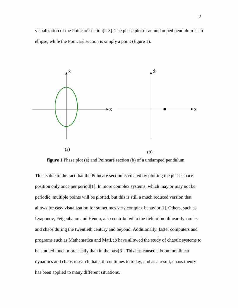
visualization of the Poincaré section[2-3]. The phase plot of an undamped pendulum is an

ellipse, while the Poincaré section is simply a point (figure 1).

This is due to the fact that the Poincaré section is created by plotting the phase space

position only once per period[1]. In more complex systems, which may or may not be

periodic, multiple points will be plotted, but this is still a much reduced version that

allows for easy visualization for sometimes very complex behavior[1]. Others, such as

Lyapunov, Feigenbaum and Hénon, also contributed to the field of nonlinear dynamics

and chaos during the twentieth century and beyond. Additionally, faster computers and

programs such as Mathematica and MatLab have allowed the study of chaotic systems to

be studied much more easily than in the past[3]. This has caused a boom nonlinear

dynamics and chaos research that still continues to today, and as a result, chaos theory

has been applied to many different situations.

(a) (b)

figure 1 Phase plot (a) and Poincaré section (b) of a undamped pendulum

3

1.3 Applications

The methods developed by Poincaré and others are used to study chaotic behavior

in a wide variety of systems including models of the behavior of the heart, changes in

biological populations due to predator-prey interaction, fluctuations in financial

markets[2-3], and the ionization of molecules under the influence of a magnetic field [4].

Chaos can occur in all of these systems because it only requires two main properties:

sensitivity to initial conditions and sensitivity to a parameter. Neither high dimension nor

complex equations are needed for chaos. Many one-dimensional systems, such as the

logistic map, behave chaotically[3].

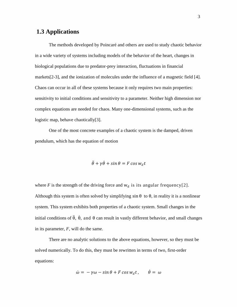
One of the most concrete examples of a chaotic system is the damped, driven

pendulum, which has the equation of motion

𝜃 + 𝛾𝜃 + 𝑠𝑖𝑛 𝜃 = 𝐹 𝑐𝑜𝑠 𝑤𝑑𝑡

where F is the strength of the driving force and wd is its angular frequency[2].

Although this system is often solved by simplifying sin θ to θ, in reality it is a nonlinear

system. This system exhibits both properties of a chaotic system. Small changes in the

initial conditions of θ , θ , and θ can result in vastly different behavior, and small changes

in its parameter, F, will do the same.

There are no analytic solutions to the above equations, however, so they must be

solved numerically. To do this, they must be rewritten in terms of two, first-order

equations:

𝜔 = − 𝛾𝜔 − 𝑠𝑖𝑛 𝜃 + 𝐹 𝑐𝑜𝑠 𝑤𝑑𝑡 , 𝜃 = 𝜔

4

The solutions can then be plotted by a program, either in real space or in phase space.

Chaotic systems can give rise to varying phenomena, such as chaotic attractors and

tangles[2-3]. There are two types of tangles: homoclinic and heteroclinic[5]. Because the

area preserving Hénon map creates a homoclinic tangle, I will be focusing on this type.

1.4 Homoclinic Tangles

Homoclinic tangles are complex objects, so to understand what they are, it is first

helpful to understand their components. Homoclinic tangles are made up of stable and

unstable manifolds attached to a fixed point[5]. In one dimension, a fixed point can be

stable if nearby points move towards it, or unstable if nearby points fly away from it. A

stable fixed point occurs at the minimum of a damped harmonic oscillator—a pendulum

will always come to rest straight down if no forces are applied. An unstable fixed point

can be visualized as a ball at the top of a hill: small perturbations away from the fixed

point will result in the ball falling off (figure 2a). In two-dimensions, fixed points are a

little more complicated. Stable fixed points must be stable in all directions, which is

basically the same idea as in one dimension. However, unstable fixed points occur in two

varieties.

(b) (a)

figure 2 (a) Small perturbations will result in large movement away from an unstable

fixed point, such as a ball on top of a hill. (b) A hyperbolic fixed point with stable (red)

and unstable (blue) directions.

5

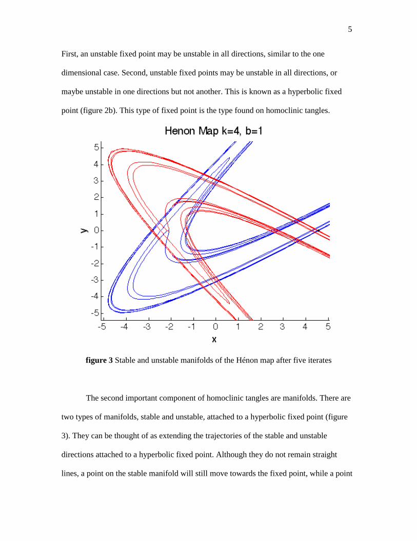
First, an unstable fixed point may be unstable in all directions, similar to the one

dimensional case. Second, unstable fixed points may be unstable in all directions, or

maybe unstable in one directions but not another. This is known as a hyperbolic fixed

point (figure 2b). This type of fixed point is the type found on homoclinic tangles.

figure 3 Stable and unstable manifolds of the Hénon map after five iterates

The second important component of homoclinic tangles are manifolds. There are

two types of manifolds, stable and unstable, attached to a hyperbolic fixed point (figure

3). They can be thought of as extending the trajectories of the stable and unstable

directions attached to a hyperbolic fixed point. Although they do not remain straight

lines, a point on the stable manifold will still move towards the fixed point, while a point

6

on the unstable manifold will move away. A manifold can never cross itself, which

results in their winding behavior, but unstable and stable manifolds will intersect an

infinite number of times. This complicated bending and twisting gives rise to the name

“tangle.”

Homoclinic tangles consist of infinitely long portions of stable and unstable

manifolds attached to a single fixed point. For clarity, only a short portion of the stable

manifold is usually pictured, while the unstable manifold is computed for longer lengths

(figure 4). Information about the dynamics of the system can be determined by properties

of the tangles, and more information is acquired as the system is iterated further. There is

another type of tangle known as the heteroclinic tangle, which involves the manifolds of

two fixed points interacting, but this type will not be covered.

figure 4 The Hénon map after many iterates

7

1.5 The Hénon map

One of the simplest two-dimensional chaotic systems is the Hénon map, which is

given by the two equations

𝑥𝑛+1 = 𝑦𝑛 − 𝑘 + 𝑥𝑛2

𝑦𝑛+1 = −𝑏𝑥𝑛

Different from the damped, driven pendulum example, which is continuous in time, the

Hénon map is an iterated map, or discrete in time, that maps the (x,y) plane onto itself

and exhibits chaotic behavior[2-3]. It was created by Michel Hénon as a simplification of

the Poincaré section of the Lorenz system [2] and has since then been studied a great deal

because of its ease of computation and interesting behavior.

The canonical version of the Hénon map has b < 1, so the area shrinks after each

iterate. It also has a fixed k value. The most interesting property of the canonical Hénon

map is its chaotic attractor[2-3]. Similar to a fixed point, points nearby the attractor will

move towards it and eventually follow its path. However, a chaotic attractor is not made

up of one point, but is instead a complex pattern. This version of the Hénon map has been

very well studied, but there are many other types. In addition, there are many other two-

dimensional maps that exhibit chaotic behavior, such as the standard map and the Baker

map [2].

1.6 Topological Entropy

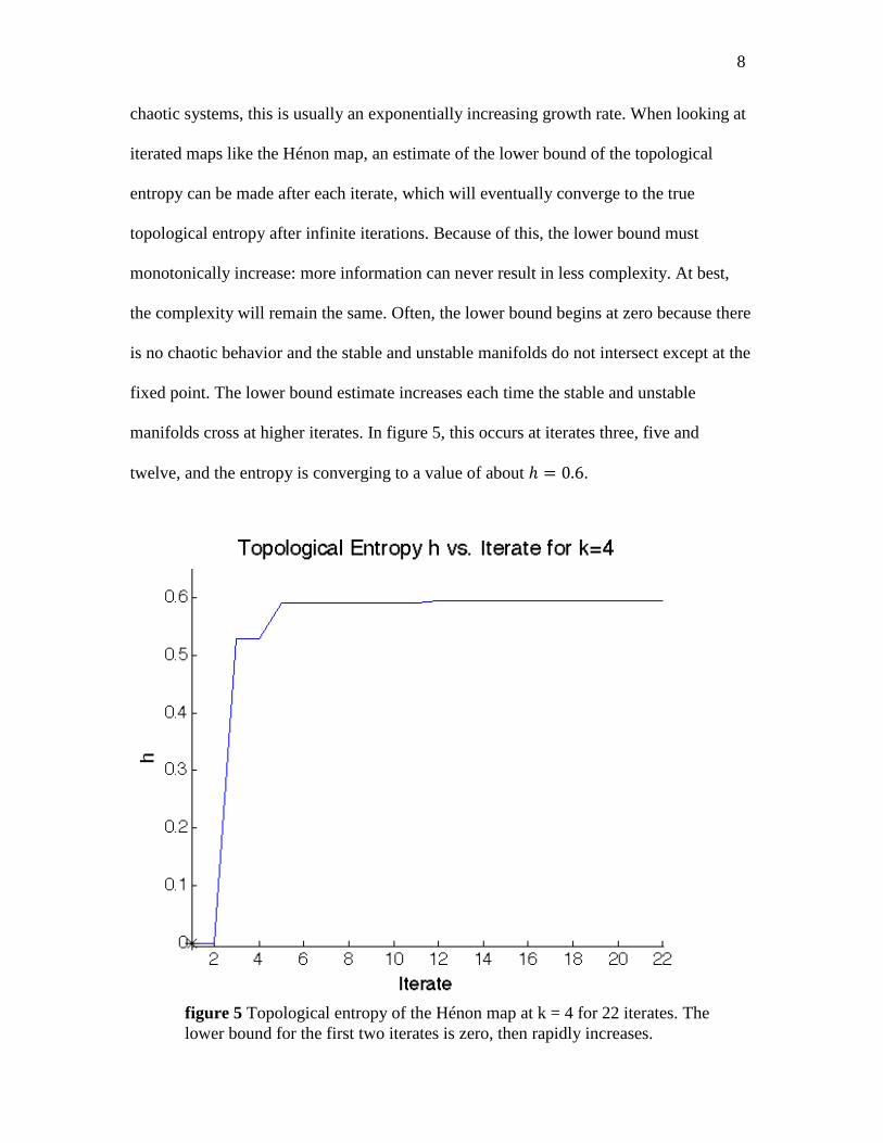
One good way to measure the complexity of a homoclinic tangle is to look at its

topological entropy: the more complex a system is, the more topological entropy it will

have. The topological entropy of a system is related the growth rate of a material line. In

8

chaotic systems, this is usually an exponentially increasing growth rate. When looking at

iterated maps like the Hénon map, an estimate of the lower bound of the topological

entropy can be made after each iterate, which will eventually converge to the true

topological entropy after infinite iterations. Because of this, the lower bound must

monotonically increase: more information can never result in less complexity. At best,

the complexity will remain the same. Often, the lower bound begins at zero because there

is no chaotic behavior and the stable and unstable manifolds do not intersect except at the

fixed point. The lower bound estimate increases each time the stable and unstable

manifolds cross at higher iterates. In figure 5, this occurs at iterates three, five and

twelve, and the entropy is converging to a value of about ℎ = 0.6.

figure 5 Topological entropy of the Hénon map at k = 4 for 22 iterates. The

lower bound for the first two iterates is zero, then rapidly increases.

9

Because topological entropy is related to complexity, it can be used to compare

maps at different parameter values, which can have drastically different behavior even

when the change in parameter is small due to their chaotic nature. The appearance of new

fixed points and periodic orbits at certain parameter values can make the system more

complex, but sometimes their effects are not immediately obvious. The topological

entropy may give hints at when a periodic orbit starts to affect the system, and may allow

for a way to visualize the changing complexity of the system as a whole as parameters are

varied.

10

Chapter 2

Topological Entropy Over a Range of k Values

2.1 The Hénon Map Revisited

As explained previously, the Hénon map is a well-studied map that exhibits

chaotic behavior with the simple set of equations:

𝑥𝑛+1 = 𝑦𝑛 − 𝑘 + 𝑥𝑛2

𝑦𝑛+1 = −𝑏𝑥𝑛

where 𝑏 and 𝑘 are the parameters of the map. For the purposes of our simulations, we set

𝑏 = 1 and varied the k values from 𝑘 = 2 to 𝑘 = 4.5 in increments of 0.01. When 𝑏 =

1, the Hénon map is area-preserving. This means that the map neither stretches or shrinks

after each iterate, and the manifolds behave somewhat like trajectories in real space.

When 𝑏 = 1 the Hénon map is also invertible, allowing for the calculation of the stable

manifold by inverting the Hénon map:

𝑥𝑛−1 = −1

𝑏𝑦𝑛

𝑦𝑛−1 = 𝑥𝑛 + 𝑘 − (1

𝑏𝑦𝑛)2

When 𝑏 = 1, the Hénon map can be thought of as a simple model for ionization: chaotic

behavior occurs inside the tangle, while a particle escapes when it crosses the stable

manifold.

11

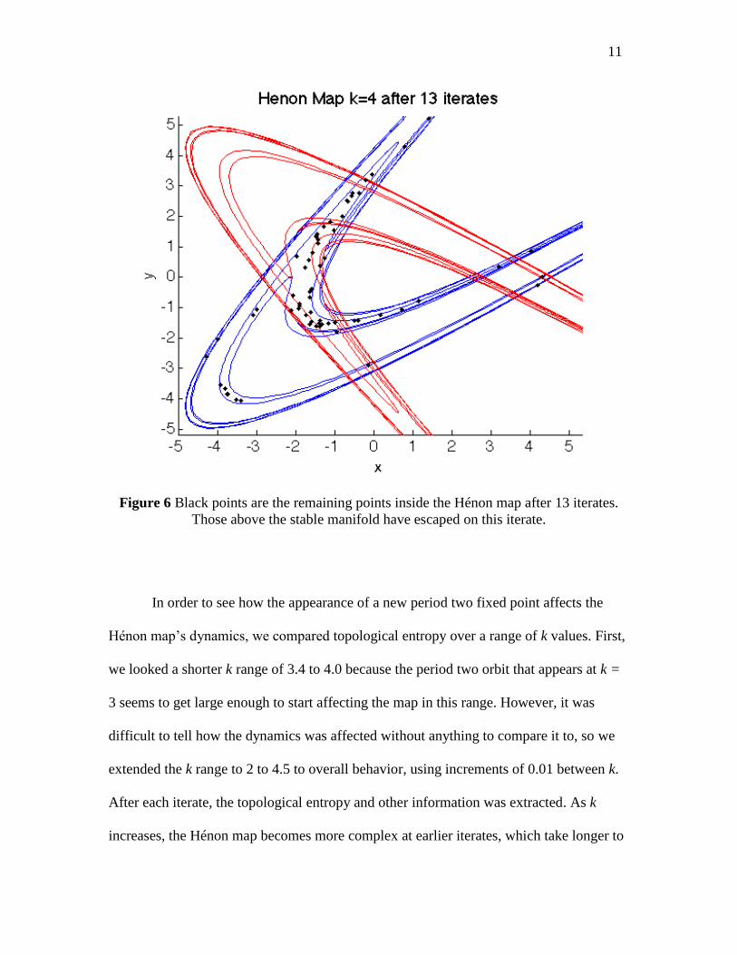
Figure 6 Black points are the remaining points inside the Hénon map after 13 iterates.

Those above the stable manifold have escaped on this iterate.

In order to see how the appearance of a new period two fixed point affects the

Hénon map’s dynamics, we compared topological entropy over a range of k values. First,

we looked a shorter k range of 3.4 to 4.0 because the period two orbit that appears at k =

3 seems to get large enough to start affecting the map in this range. However, it was

difficult to tell how the dynamics was affected without anything to compare it to, so we

extended the k range to 2 to 4.5 to overall behavior, using increments of 0.01 between k.

After each iterate, the topological entropy and other information was extracted. As k

increases, the Hénon map becomes more complex at earlier iterates, which take longer to

12

compute. Because of this, an area cutoff was added which stopped the program after the

area between two segments of unstable manifold become too close together. This caused

the results for different k values to run for different amount of iterates. In addition,

intersection errors in the unstable manifold sometimes caused the program to stop early,

but each k value yielded at least ten iterates worth of data for comparison.

2.2 Single k Entropy Results

Plotting entropy for a single k value results in a graph such as figure 7. The first

lower bound of entropy is always zero because there is essentially no complexity to the

system. The second value is also always zero for our range of k because it does not

increase complexity enough to affect anything. After the third iterate, the lower bound is

increased to around 0.53 for all k in this range. However, after the third iterate, the

behavior of the topological entropy becomes much more unpredictable. In addition, there

Figure 7 topological entropy vs. iterate for k=3.35

iterate

Topolo

gic

al E

ntr

opy h

k = 3.35

13

Figure 8 Using normalized entropy differences highlights small changes in h

may be small changes in entropy that are difficult to see by inspecting the entropy plots.

In order to see smaller changes in entropy more easily, a normalized entropy

difference can be used. In this case, we used the equation

ln[(𝑒ℎ𝑓−𝑒ℎ𝑛 )/𝑒ℎ𝑓 ]

to highlight small changes in entropy as in figure 8. This reveals that for some k values

there are many, very small changes in entropy between iterates 10 to 25 not seen in the

original entropy plot. The ideal way to graph over large k ranges would show how these

small changes in entropy are affected by changing k values.

14

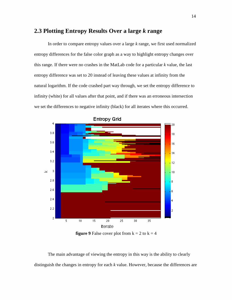
2.3 Plotting Entropy Results Over a large k range

In order to compare entropy values over a large k range, we first used normalized

entropy differences for the false color graph as a way to highlight entropy changes over

this range. If there were no crashes in the MatLab code for a particular k value, the last

entropy difference was set to 20 instead of leaving these values at infinity from the

natural logarithm. If the code crashed part way through, we set the entropy difference to

infinity (white) for all values after that point, and if there was an erroneous intersection

we set the differences to negative infinity (black) for all iterates where this occurred.

figure 9 False cover plot from k = 2 to k = 4

The main advantage of viewing the entropy in this way is the ability to clearly

distinguish the changes in entropy for each k value. However, because the differences are

15

normalized compared with each k value’s final entropy, it is difficult to compare changes

between k values. Although some general trends are noticeable, such as the relatively

steady entropy trend at low k, other trends are not. In addition, regions of

nonmonotonicity are usually not noticeable in this graph, which makes it difficult to

discern where the code has errors. This is especially difficult to see when looking over a

large range of k values.

Although the previous graph allowed us to see generally where entropy changed,

we needed to find a better way to see where larger jumps in entropy occurred. In order to

do this, we plotted 𝑒ℎ for each k value on the same graph. Setting low k to green and high

k to blue, we can see that lower bound estimates jump to higher values at earlier iterates

as k increases. Details are difficult to make out in some sections where entropy is

Figure 10 All entropy plots for k = 2 to k = 4.5 in increments of 0.01 Green

is low k while blue is high k

16

changing slightly at each k, but it is easier to figure out where these sections are and take

a closer view of them with this method.

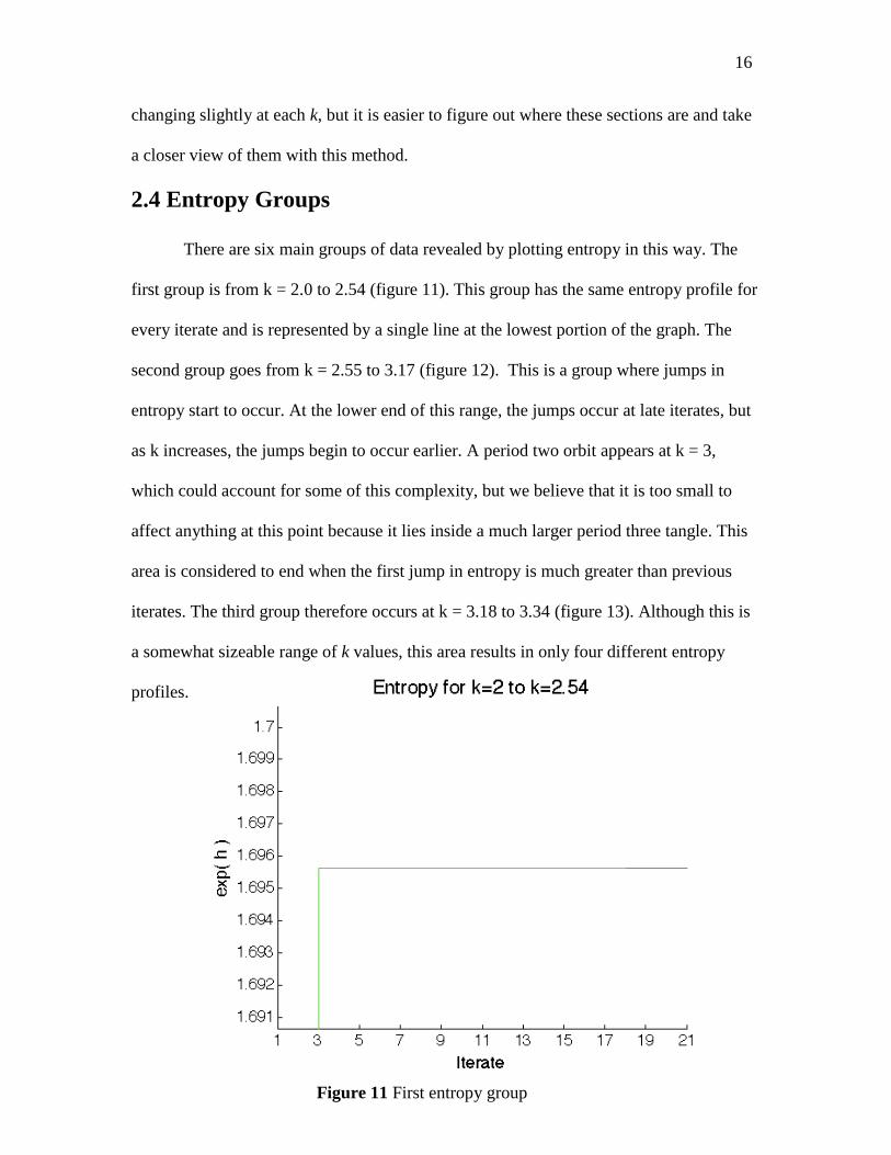
2.4 Entropy Groups

There are six main groups of data revealed by plotting entropy in this way. The

first group is from k = 2.0 to 2.54 (figure 11). This group has the same entropy profile for

every iterate and is represented by a single line at the lowest portion of the graph. The

second group goes from k = 2.55 to 3.17 (figure 12). This is a group where jumps in

entropy start to occur. At the lower end of this range, the jumps occur at late iterates, but

as k increases, the jumps begin to occur earlier. A period two orbit appears at k = 3,

which could account for some of this complexity, but we believe that it is too small to

affect anything at this point because it lies inside a much larger period three tangle. This

area is considered to end when the first jump in entropy is much greater than previous

iterates. The third group therefore occurs at k = 3.18 to 3.34 (figure 13). Although this is

a somewhat sizeable range of k values, this area results in only four different entropy

profiles.

Figure 11 First entropy group

17

Figure 12 Second entropy group

Figure 13 Third entropy group

18

The fourth group occurs between k = 3.35 to 3.74. This is the second main area

when complexity starts to creep in from high iterates. It is difficult to see on the plot over

all k values, so it is helpful to look at it on its own. This also shows that entropy is self-

similar because this view looks much the same as the total view. This group also shares

another feature, which is that the second jump in entropy occurs at the eleventh iterate.

Once again, as k increases the jumps in entropy start occurring at earlier and earlier

iterates.

The next two sections are areas of relative little activity. The fifth consists of k =

3.74 to 3.98, all of which have a second jump in entropy at the seventh iterate. The final

Figure 14 Fourth entropy group (a) full

view and (b) zoomed view.

(a) (b)

19

group occurs from k = 3.99 to 4.5, where the second jump in entropy occurs at iterate

five. Although the second jumps occur on different iterates, otherwise these two sections

behave relatively the same. In addition, many of the runs in the last section ended early,

so there may be more information that isn’t pictured in this graph that appears at late

times.

Figure 15 Fifth entropy group

Figure 16 Sixth entropy group

20

These changes in how entropy jumps at different iterates can be viewed as

“entropy fronts” coming in from late times to earlier times. For example, as the second

group transitions into the first group, all the complexity that appeared in small jumps now

appears in one large jump at k = 3.18, and then remains relatively flat. Another place to

easily picture an entropy front coming in is between the fifth and sixth groups. In the fifth

group, all k values jump up at the fifth iterate, whereas in the sixth group all k values

jump immediately up to an even higher value at the fourth iterate.

These entropy fronts are useful for looking at where changes in k result in large

jumps in entropy. In addition, there are times one k value has many small changes at high

iterates, while the next k value only 0.01 away may only have one, larger jump in entropy

for the same iterate interval. One reason this occurs is that the Hénon map become larger

as k increases, so that more information is revealed on each iterate. However, this alone

does not explain how the small changes occur.

21

Chapter 3

Conclusions

3.1 Entropy Fronts

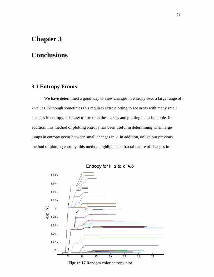
We have determined a good way to view changes in entropy over a large range of

k values. Although sometimes this requires extra plotting to see areas with many small

changes in entropy, it is easy to focus on these areas and plotting them is simple. In

addition, this method of plotting entropy has been useful in determining when large

jumps in entropy occur between small changes in k. In addition, unlike our previous

method of plotting entropy, this method highlights the fractal nature of changes in

Figure 17 Random color entropy plot

22

entropy. Because the Hénon map is chaotic, this behavior was not all that unexpected, but

it useful to tell where changes occur.

Graphing topological entropy in this way allowed us to see the entropy front

pattern. Although we could tell that the entropy increased quicker for higher k values, we

can now look at specific areas where the entropy is changing more rapidly. One grouping

in particular, from k = 3.35 to 3.73, seems to stem from the period two orbit becoming

large enough to influence the system as a whole early on. The second group, k = 2.55 to

3.17, may also arise from a periodic orbit, although we don’t know if this is the case.

3.2 Errors

There were three main types of errors that occurred while running simulations.

The first was an error that caused the simulation to stop running prematurely. This error

did not affect any of the results significantly. The second error was caused when the

simulation resulted in intersections between two pieces of unstable manifold. Although

Figure 18 Nonmonotonic runs

23

this did not appear to affect the topological entropy, it did affect other quantities such as

the number of symbols. The third type of error that occurred was that the entropy values

had some nonmonotonic sections. This usually occurred for one or two consecutive

values per k value that contained errors. Some of these nonmonotonic runs appear to

follow the same profile as a nearby monotonic run, and in these cases it appears that only

one value was incorrectly calculated. Other nonmonotonic runs were very small (less

than 10-13

) and were probably the result of round-off error during simulation. Overall,

there were 31 nonmonotonic runs out of 251 total runs that cannot be attributed to round-

off error.

3.3 Future directions

There are many more potential areas to study in the Hénon map. One step that

would improve this research would be finding out what causes the nonmontonicity and

other errors. In addition, improving the matlab code to run more efficiently would allow

for quicker analysis so that data could be taken more easily. However, this is a relatively

minor issue, and more important aspects of this project can still be focused on in the

future.

First, entropy fronts can be explored in more detail. Although there is a general

trend of starting at late iterates for smaller k and coming in at early iterates for larger k

values, more k values could be explored to see if this trend holds or if new patterns

emerge. Also, the groups where entropy fronts come in rapidly, such as k = 2.55 to 3.17

group and the 3.35 to 3.73 group, could be looked at more closely to see if they correlate

with the appearance of new periodic orbits. A larger k range could be inspected if some

correlations are found to see if they hold for more values.

24

Secondly, the same k range could be reevaluated with a smaller area threshold to

further explore late iterates. Allowing late-time behavior could show additional structure,

especially for those values that showed no addition structure for all iterates examined. It

could also reveal more information on higher k values since increasing the area threshold

sometimes reduces the errors in computation that cause the code to stop early. If new

complexities are then discovered, these may also be correlated to other values.

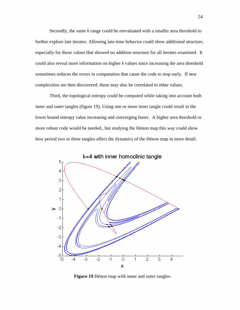
Third, the topological entropy could be computed while taking into account both

inner and outer tangles (figure 19). Using one or more inner tangle could result in the

lower bound entropy value increasing and converging faster. A higher area threshold or

more robust code would be needed., but studying the Hénon map this way could show

how period two or three tangles affect the dynamics of the Hénon map in more detail.

Figure 19 Hénon map with inner and outer tangles.

25

Finally, other information from the Hénon map could be compared over a similar

range of k values. Because new periodic orbits occur quite often, trends in the

appearances of these periodic orbits could be observed. Another measure of complexity

might be the minimum number of symbols needed to describe the map at a given iterate.

The current code used obtains much more information than the topological entropy alone,

and this information could hold a key to discovering patterns in the behavior of the

Hénon map. If discovered, these patterns could eventually lead to generalities that apply

to more realistic models and could possibly lead to a deeper understanding of chaotic

systems. Additionally, the Hénon map and other simple maps could be used as a test

model to verify new theories about dynamical systems that may arise. These

advancements would likely be some time in the future, but even a simple model like the

Hénon map still may help find them.

26

References

1. Nolte, D.D. “The Tangled Tale of Phase Space”. (2010), Physics Today,

63(4) pp. 33-38 .

2. Ivancevic, V.G., Ivancevic, T.T. “Basics of Nonlinear and Chaotic

Dynamics”, Complex Nonlinearity: Chaos, Phase Transitions, Topology

Change and Path Integrals. Berlin, Springer (2008).

3. Alligood, K.T. Sauer, T.D., Yorke, J.A. “Two-Dimensional Maps”. Chaos: An

Introduction to Dynamical Systems. New York, Springer (1996)

4. Mitchell K.A., Hendley, J.P., Tighe, B., Flower, A. Delos J.B. “Chaos-

Induced Pulse Trains in the Ionization of Hydrogen” (2004) Physical Review

Letters 92 (7) np

5. Mitchell K.A. “The topology of nested homoclinic and heteroclinic tangles”

(2009) Physica D: Nonlinear Phenomena, 238 (7), pp. 737-763.